entrainment, diapycnal mixing and transport in three ... · entrainment, diapycnal mixing and...
TRANSCRIPT

Ocean Modelling 9 (2005) 151–168
www.elsevier.com/locate/ocemod
Entrainment, diapycnal mixing and transportin three-dimensional bottom gravity current simulations using
the Mellor–Yamada turbulence scheme
Tal Ezer *
Program in Atmospheric and Oceanic Sciences, Princeton University, Princeton, NJ 08544-0710, USA
Received 30 March 2004
Available online 25 June 2004
Abstract
The diapycnal mixing, entrainment and bottom boundary layer (BBL) dynamics in simulations of dense
overflows are evaluated, using a generalized coordinate ocean model that can utilize terrain-following or
z-level vertical grids and uses the Mellor–Yamada (M–Y) turbulence closure scheme to provide vertical
mixing coefficients. Results from idealized dense water overflow experiments at resolutions of 10 and 2.5 kmusing a terrain-following vertical coordinates compare very well with the results from a nonhydrostatic
ocean model (MITgcm) with resolution of 0.5 km, and also with the basic observed properties of the
Denmark Straits overflow. At both 10 and 2.5 km resolutions the dilution of the bottom plume is com-
parable to the nonhydrostatic results, indicating that the M–Y scheme represents the subgrid-scale mixing
very well. The 2.5 and 0.5 km model simulations are surprisingly very similar even in the details of the eddy
field structure. Strong diapycnal mixing and large entrainment result in more than doubling the plume
transport within �100 km from the source, similar to observations, while further downstream small
detrainment and reduced transport occur. However, when the diapycnal mixing associated with the mixingscheme is eliminated by setting KH ¼ 0, the terrain-following model results closely resemble the results of
isopycnal models whereas the dense plume slides farther downslope while its transport continue to increase
indefinitely. On the other hand, when eliminating the bottom Ekman transport associated with the mixing
scheme by setting KM ¼ 0, the model results resemble the results of a stepped-topography z-level model
without BBL. The bottom Ekman transport associated with the M–Y vertical mixing was found to be
responsible for �20% of the downslope transport of the bottom plume. The vertical mixing coefficient
shows a spatially variable asymmetric structure across the bottom plume indicating a stronger mixing over
* Tel.: +1-609-258-1318; fax: +1-609-258-2850.
E-mail address: [email protected] (T. Ezer).
1463-5003/$ - see front matter � 2004 Elsevier Ltd. All rights reserved.
doi:10.1016/j.ocemod.2004.06.001

152 T. Ezer / Ocean Modelling 9 (2005) 151–168
a thicker BBL in the upslope side of the plume, and a weaker mixing over a thinner BBL in the downslope
side of the plume.
� 2004 Elsevier Ltd. All rights reserved.
Keywords: Numerical modeling; Overflow; Ocean mixing
1. Introduction
Recent observations (Girton and Sanford, 2003) and laboratory experiments (Cenedese et al.,2004) of dense overflow gravity currents and their interaction with sloping bottoms indicatecomplex flow dynamics that may involve eddies, bottom mixing and entrainment. For examplethe mixing characteristics and spreading of the Denmark Strait overflow show highly variablecurrents with strong entrainment and transport changes within �100–200 km from the sill (Girtonand Sanford, 2003). It is a great challenge for ocean models, in particular for coarse resolutionclimate models, to accurately simulate such flows, whereas overflow simulations largely depend onthe model configuration and the subgrid-scale mixing parameterization (Griffies et al., 2000).
The representation of topography in coarse resolution climate models may also be a challenge.The difficulty in simulating overflow processes using z-level grids with stepped topography hasbeen indicated in numerous studies (Gerdes, 1993; Beckmann and D€oscher, 1997; Winton et al.,1998; Pacanowski and Gnanadesikan, 1998; Griffies et al., 2000; Ezer and Mellor, 2004).Therefore, various ways of either improving the bottom representation in models (Adcroft et al.,1997; Pacanowski and Gnanadesikan, 1998) or adding various bottom boundary layer (BBL)schemes (Beckmann and D€oscher, 1997; Campin and Goosse, 1999; Killworth and Edwards,1999; Song and Chao, 2000) have been developed. However, those BBL schemes do not com-pletely solve the problem, and may need numerical improvements or calibration. Overflowsrepresentation in terrain-following ocean models (Jiang and Garwood, 1996; Jungclaus andMellor, 2000; K€ase et al., 2003; Jungclaus et al., 2001) and in isopycnal ocean models (Papadakiset al., 2002) may seem easier to achieve since bottom plumes to large extent are driven by theirdensity anomaly relative to the background stratification, and the flow is mostly parallel to thebottom. Nevertheless, finding appropriate parameterizations for diapycnal mixing in hydrostaticmodels of all types is still an area of ongoing research (Price and Barringer, 1994; Griffies et al.,2000; Hallberg, 2000; Papadakis et al., 2002; Legg et al., in press).
While using very high resolution (<1 km grids) nonhydrostatic ocean models (Marshall et al.,1998; Ozgokmen and Chassignet, 2002; Legg et al., in press) for large scale problems may still beimpractical, they can be used for comparison and calibration of mixing parameterizations incoarser resolution models. The dynamics of overflows mixing and entrainment (DOME) initiativeestablished an idealized model setup to investigate the dynamics of bottom plumes and aframework to compare different models. For example, the DOME setup was used to compareterrain-following and z-level models (Ezer and Mellor, 2004), and to compare isopycnal andz-level models as well as hydrostatic and nonhydrostatic models (Legg et al., in press). The sameconfiguration will be used here as well.
Ezer and Mellor (2004) used the generalized coordinate model of Mellor et al. (2002) withthe Mellor–Yamada (M–Y) turbulence scheme (Mellor and Yamada, 1982). They show that a
T. Ezer / Ocean Modelling 9 (2005) 151–168 153
terrain-following model provides reasonable simulations of overflows in basin-scale (100 km grid)and in regional (10 km grid) simulations, but the M–Y mixing was not working well with astepped-topography z-level grid (10 km horizontal resolution), resulting in excess diapycnalmixing and insufficient downslope penetration of the dense plume. With 2.5 km z-level grid theBBL structure starts converging toward the terrain-following model solution and closer to thestructure of observed overflows. Adding shaved cells as in Legg et al. (in press) or any of the otherBBL parameterizations may improve the simulations of overflows in the z-level calculationswithout the need to increase resolution that much, but there are still some numerical problems orcalibration issues in those BBL schemes that are not completely resolved.
This study is a follow-up on Ezer and Mellor (2004), using the same model and configuration,but adding experiments, first with higher resolution (2.5 km) terrain-following grid that arecompared with the nonhydrostatic calculations of Legg et al. (in press), and second, special casesto isolate the effect of the M–Y turbulence scheme on diapycnal mixing and transport of thebottom plume. Countless studies looked at the M–Y scheme’s influence on shallow regions,surface mixed layers and compared it with other mixing schemes (Martin, 1985; Ezer, 2000;Warner et al., in press), but very few studies looked at its influence on the BBLs of the deep ocean.One example is the modeling study of the interaction between bottom plumes and the slopingbottom in the deep (at 4000–5000 m) North Atlantic ocean by Ezer and Weatherly (1990) whofound large spatial variations in the mixing coefficient near the bottom due to changes in strat-ification and shear across the plume. Similar BBL processes may apply to dense overflow plumes,which is the focus of this study.
2. The ocean model and the DOME setup
The Princeton ocean model with generalized coordinate system (POMgcs) is described in detailby Mellor et al. (2002). Unlike the original free surface, three-dimensional, primitive equationPOM code (Blumberg and Mellor, 1987), which used a standard vertical sigma coordinates withthe same relative layer thickness independent of depth, this version allows almost any combi-nation of terrain-following or z-level distribution of layers that may vary in space and time (i.e., anadaptable grid). The so called s-coordinate system (Song and Haidvogel, 1994) used in the re-gional ocean modeling system, ROMS, and in other terrain-following models (Haidvogel et al.,2000; Ezer et al., 2002) can be a special case of the generalized coordinates; a standard z-level gridwith stepped topography is another possible option.
The idealized model configuration for the DOME setup is described in detail in Ezer andMellor (2004) and in Legg et al. (in press). The domain includes a basin of 1100· 800 km withmaximum depth of 3600 m and a 1% steep slope which connects to a 100 km wide and 600 m deepembayment where a dense overflow of 5 Sv (1 Sverdrup ¼ 106 m3 s�1) is imposed over back-ground stratification (Fig. 1). The imposed dense inflow is in a geostrophic balance to minimizeinstability and excess mixing within the embayment. A linear equation of state (with constantsalinity) is used so that the maximum density difference (qmax � qmin in Fig. 1b) between thesurface and the deepest layers, and between the surface and the dense bottom layer in theembayment both have DrT ¼ 2 kgm�3. All grids use 50 vertical layers except the high resolutionz-level grid which used 88 layers (see Ezer and Mellor, 2004, for grids detail). To help analyze the

200
0
-200
-400
-600
(a) Model Domain and TopographyY(
km)
X(km)-600 -400 -200 0 200
600m
1600m
2600m
3600m
3600m
-600 -400 -200 0 200Y(km)
max
max
min
(z)
-600
-1800
-3000
Z(m
)
(b) Initial Stratificationρ
ρ
ρ
ρ
Fig. 1. (a) Top view of the model domain and bottom topography, and (b) side view of a cross-sections at x ¼ 0 and the
initial stratification.
154 T. Ezer / Ocean Modelling 9 (2005) 151–168
development of the dense water plume, a tracer, with value c ¼ 1, was injected into the densewater in the embayment; initially c ¼ 0 everywhere else.
Constant horizontal diffusivity (AH) and viscosity (AM ¼ 5AH) are used with values of AH ¼ 10m2 s�1 for the 2.5 km grids and AH ¼ 100 m2 s�1 for the 10 km grids (see Ezer and Mellor, 2004,for model sensitivity to diffusivity values in overflow simulations). The vertical mixing coefficientsare obtained from the Mellor–Yamada turbulence scheme (Mellor and Yamada, 1982),
ðKM;KHÞ ¼ ‘qðSM; SHÞ; ð1Þ
with the turbulence kinetic energy, q2=2 and the turbulence length scale, ‘, are calculated from twoprognostic equations that take into account horizontal and vertical diffusion, shear and buoyancyproduction and turbulence dissipation. SM and SH are stability functions which depend on theRichardson number. A small background vertical diffusivity of 2· 10�5 m2 s�1 is added to (1),however, in the special experiments where mixing coefficients are null, the background value wasalso set to zero.
3. Results
3.1. The effect of vertical grid type and horizontal resolution on the bottom plume structure
A comparison between the terrain-following and the z-level coordinates for the DOMEexperiments using 10 km horizontal grids have been discussed in detail in Ezer and Mellor (2004).In Fig. 2, additional experiments with the two coordinate types using 2.5 km grids are alsocompared with results of the nonhydrostatic MIT general circulation model (MITgcm) which usesa 0.5 km horizontal grid. Note however, that even at 0.5 km resolution the nonhydrostatic modeldoes not fully resolve shear instability mixing at the interface of the plume and the ambient layers,so it may be called a ‘‘mixing permitting’’, not a ‘‘mixing resolving’’ model (Legg et al., in press).Several interesting points emerge from this comparison.
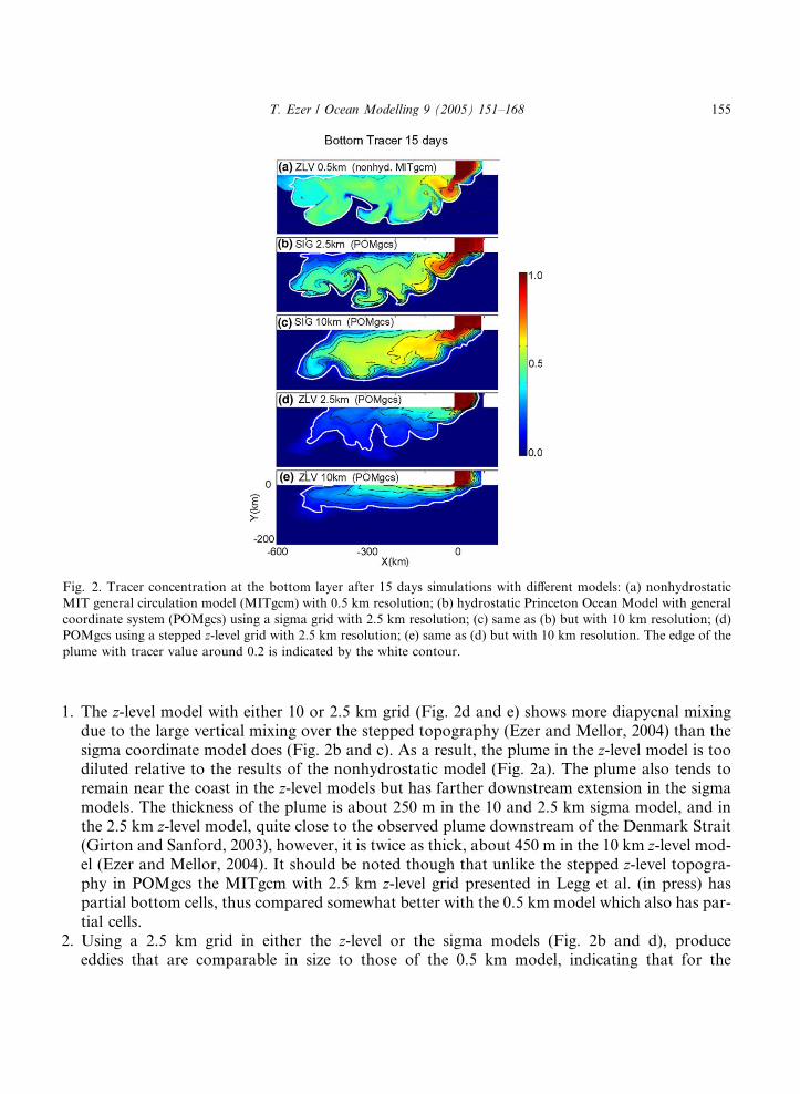
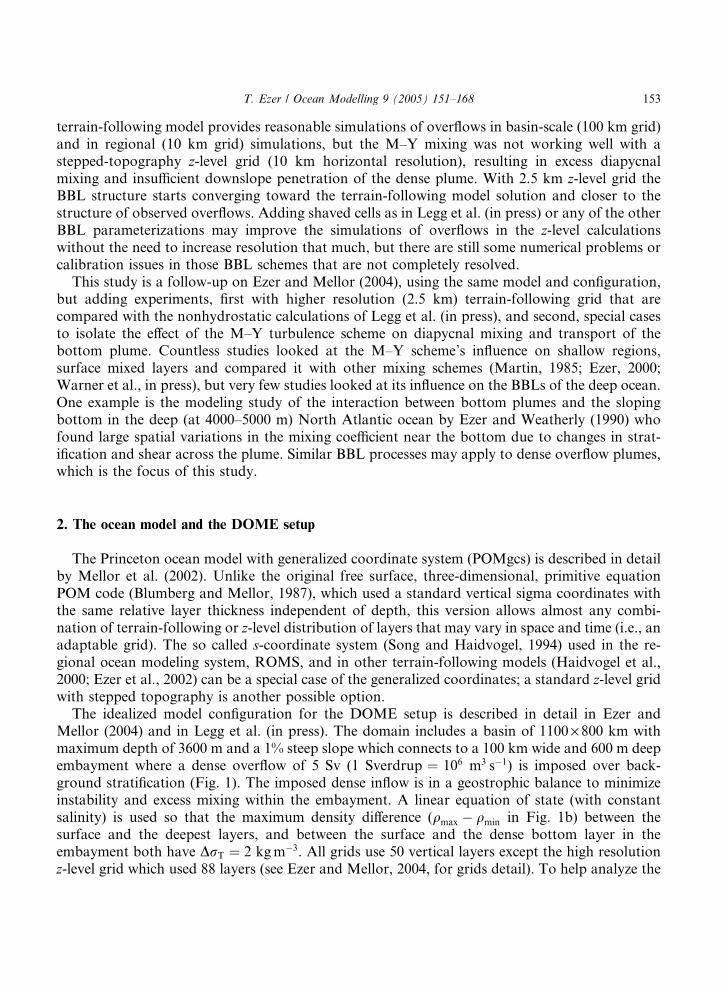
Fig. 2. Tracer concentration at the bottom layer after 15 days simulations with different models: (a) nonhydrostatic
MIT general circulation model (MITgcm) with 0.5 km resolution; (b) hydrostatic Princeton Ocean Model with general
coordinate system (POMgcs) using a sigma grid with 2.5 km resolution; (c) same as (b) but with 10 km resolution; (d)
POMgcs using a stepped z-level grid with 2.5 km resolution; (e) same as (d) but with 10 km resolution. The edge of the
plume with tracer value around 0.2 is indicated by the white contour.
T. Ezer / Ocean Modelling 9 (2005) 151–168 155
1. The z-level model with either 10 or 2.5 km grid (Fig. 2d and e) shows more diapycnal mixingdue to the large vertical mixing over the stepped topography (Ezer and Mellor, 2004) than thesigma coordinate model does (Fig. 2b and c). As a result, the plume in the z-level model is toodiluted relative to the results of the nonhydrostatic model (Fig. 2a). The plume also tends toremain near the coast in the z-level models but has farther downstream extension in the sigmamodels. The thickness of the plume is about 250 m in the 10 and 2.5 km sigma model, and inthe 2.5 km z-level model, quite close to the observed plume downstream of the Denmark Strait(Girton and Sanford, 2003), however, it is twice as thick, about 450 m in the 10 km z-level mod-el (Ezer and Mellor, 2004). It should be noted though that unlike the stepped z-level topogra-phy in POMgcs the MITgcm with 2.5 km z-level grid presented in Legg et al. (in press) haspartial bottom cells, thus compared somewhat better with the 0.5 km model which also has par-tial cells.
2. Using a 2.5 km grid in either the z-level or the sigma models (Fig. 2b and d), produceeddies that are comparable in size to those of the 0.5 km model, indicating that for the

156 T. Ezer / Ocean Modelling 9 (2005) 151–168
characteristics of this overflow, with a Rossby radius of deformation of �20–50 km, a modelresolution of 2.5 km may be sufficient. The importance of meandering and eddies for mixingof overflow plumes has been indicated in previous studies using numerical models, observa-tions and laboratory experiments (Jiang and Garwood, 1996; Jungclaus et al., 2001; Girtonand Sanford, 2003; Cenedese et al., 2004). The entrainment rate and the thickness of simu-lated plumes are influenced by the ability of the model to resolve these eddies (Ezer andMellor, 2004).
3. Because of the non-linear nature of the plume dynamics and the complicated turbulent mixinginvolved in the interaction of the plume with the overlaying water and with the sloping bottom,it is somewhat surprising to see that the details of the plume structure and its dilution in the 2.5km sigma model after 15 days (Fig. 2b) are so similar to those obtained by a completely differ-ent model with a horizontal resolution five times finer and nonhydrostatic dynamics (Fig. 2a).In fact, the 2.5 km POMgcs results resemble the 0.5 km MITgcm results even more than theresults of the 2.5 km version of the same MITgcm model do (shown in Legg et al., in press).Note for example, the similarity in the ‘‘hammer head’’ like deep-water intrusion nearx ¼ �300 km. However, some differences remain––for example, the plume separated fromthe coast in the sigma model but not in the MIT model, a feature also typical to our coarserresolution z-level grid of Fig. 2e. It will be shown later that this difference may relate to theEkman transport in the BBL.
The above comparisons, and in particular point #3, indicate that the BBL mixing and theentrainment with the overlaying waters are simulated well in the sigma model when vertical(diapycnal) mixing is represented by the M–Y turbulence scheme. In the M–Y model the unre-solved subgrid-scale turbulence is solved by prognostic equations for the turbulence velocity andlength scale so there is no need for specific parameterizations of entrainment. In other modelsentrainment may be estimated for example from Richardson or Froude number parameteriza-tions (Price and Barringer, 1994; Hallberg, 2000).
Details of the structure of the plume near the bottom after 40 days (Fig. 3) reveals anasymmetric spatial structure of the mixing coefficient with large values near the north (upslope)side of the plume, where significant mixing extends for over 100 m from the bottom, but withsmaller mixing coefficient on the downslope side, where significant mixing is limited to �25 m offthe bottom. Similar asymmetry has been found in past simulations of other dense plumes onsloping bottoms (e.g., Ezer and Weatherly, 1990), and possibly in recent observations of theDenmark Straits (Fig. 6 in Girton and Sanford, 2003, indicates larger bottom flow and bottomstress on the upslope side of the plume). The reason for this asymmetry is the Ekman BBLdynamic which causes the velocity to spiral from almost along isobath in the upper plume to-ward more downslope direction near the bottom (toward the left in Fig. 3). Therefore, thedownslope Ekman transport destabilizes the stratification on the upslope side, pushing lighterbottom water of the interior under the dense plume water, the result is a large KM that creates awell mixed BBL (note the vertical density contours around x ¼ �25 km). On the other (down-slope) side of the plume, the Ekman transport pushes the dense source water under lighterinterior waters, the result is a thin and stable BBL with less vertical mixing. Note also that thedownslope edge of the plume reached the depth in which its buoyancy relative to the interior isalmost neutral.
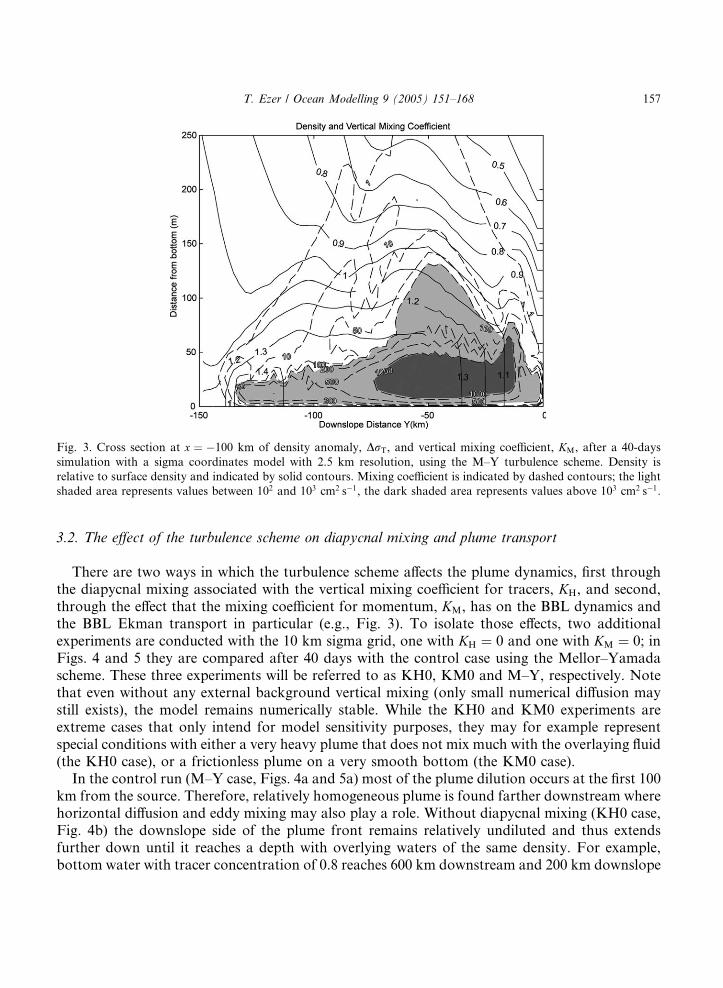
Fig. 3. Cross section at x ¼ �100 km of density anomaly, DrT, and vertical mixing coefficient, KM, after a 40-days
simulation with a sigma coordinates model with 2.5 km resolution, using the M–Y turbulence scheme. Density is
relative to surface density and indicated by solid contours. Mixing coefficient is indicated by dashed contours; the light
shaded area represents values between 102 and 103 cm2 s�1, the dark shaded area represents values above 103 cm2 s�1.
T. Ezer / Ocean Modelling 9 (2005) 151–168 157
3.2. The effect of the turbulence scheme on diapycnal mixing and plume transport
There are two ways in which the turbulence scheme affects the plume dynamics, first throughthe diapycnal mixing associated with the vertical mixing coefficient for tracers, KH, and second,through the effect that the mixing coefficient for momentum, KM, has on the BBL dynamics andthe BBL Ekman transport in particular (e.g., Fig. 3). To isolate those effects, two additionalexperiments are conducted with the 10 km sigma grid, one with KH ¼ 0 and one with KM ¼ 0; inFigs. 4 and 5 they are compared after 40 days with the control case using the Mellor–Yamadascheme. These three experiments will be referred to as KH0, KM0 and M–Y, respectively. Notethat even without any external background vertical mixing (only small numerical diffusion maystill exists), the model remains numerically stable. While the KH0 and KM0 experiments areextreme cases that only intend for model sensitivity purposes, they may for example representspecial conditions with either a very heavy plume that does not mix much with the overlaying fluid(the KH0 case), or a frictionless plume on a very smooth bottom (the KM0 case).
In the control run (M–Y case, Figs. 4a and 5a) most of the plume dilution occurs at the first 100km from the source. Therefore, relatively homogeneous plume is found farther downstream wherehorizontal diffusion and eddy mixing may also play a role. Without diapycnal mixing (KH0 case,Fig. 4b) the downslope side of the plume front remains relatively undiluted and thus extendsfurther down until it reaches a depth with overlying waters of the same density. For example,bottom water with tracer concentration of 0.8 reaches 600 km downstream and 200 km downslope

Fig. 4. Tracer concentration at the bottom layer after 40 days simulations with POMgcs using a sigma grid with 10 km
resolution: (a) vertical mixing coefficients for tracers (KH) and momentum (KM) obtained from the Mellor–Yamada
turbulence scheme (M–Y case); (b) setting KH ¼ 0 (KH0 case); (c) setting KM ¼ 0 (KM0 case).
158 T. Ezer / Ocean Modelling 9 (2005) 151–168
from the source in this case, but only 50 km from the source in the M–Y case. The lack of dia-pycnal mixing results in a very thin BBL (Fig. 5b). In the KM0 case (Fig. 4c) the undiluteddownslope side of the front is similar to the KH0 case (KH is also reduced when KM is eliminated),but the plume did not separate from the coast. A cross section of this case (Fig. 5c) reveals that athick and vertically mixed part of the plume remains near the wall. Vertical profiles of tracerconcentration, density and dowenslope velocity (Fig. 6) show that the diapycnal mixing in the M–Y case results in a thicker bottom mixed layer and a transition layer above the BBL, similar to the
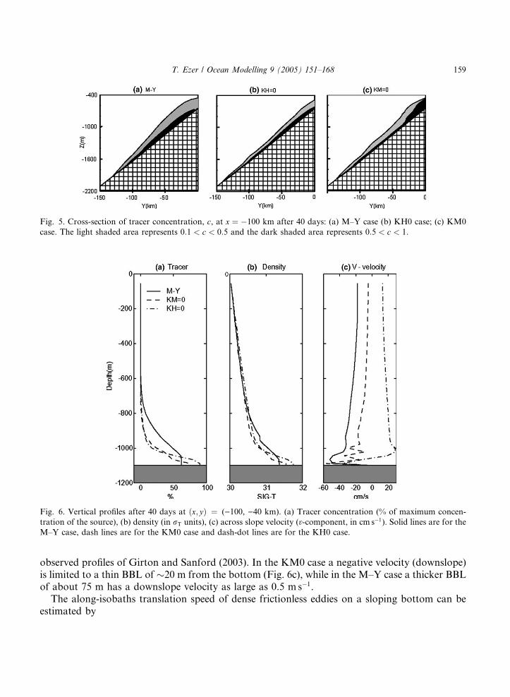
Fig. 6. Vertical profiles after 40 days at ðx; yÞ ¼ ()100, )40 km). (a) Tracer concentration (% of maximum concen-
tration of the source), (b) density (in rT units), (c) across slope velocity (v-component, in cm s�1). Solid lines are for the
M–Y case, dash lines are for the KM0 case and dash-dot lines are for the KH0 case.
Fig. 5. Cross-section of tracer concentration, c, at x ¼ �100 km after 40 days: (a) M–Y case (b) KH0 case; (c) KM0
case. The light shaded area represents 0:1 < c < 0:5 and the dark shaded area represents 0:5 < c < 1.
T. Ezer / Ocean Modelling 9 (2005) 151–168 159
observed profiles of Girton and Sanford (2003). In the KM0 case a negative velocity (downslope)is limited to a thin BBL of �20 m from the bottom (Fig. 6c), while in the M–Y case a thicker BBLof about 75 m has a downslope velocity as large as 0.5 m s�1.
The along-isobaths translation speed of dense frictionless eddies on a sloping bottom can beestimated by

160 T. Ezer / Ocean Modelling 9 (2005) 151–168
ut ¼ gDqq0
sf
ð2Þ
(Nof, 1983), where s is the bottom slope, f the Coriolis parameter, g the gravitational accelera-tion, and Dq=q0 the eddy’s density anomaly relative to the background density. Recent laboratoryexperiments show that the along-isobaths velocity component of dense overflow plumes obeys asimilar relationship (Cenedese et al., 2004). The same seems to be true for the model results. Forexample, in case KM0 (Fig. 4c) there seem to be two different downstream velocities, a faster onefor the shallow side of the plume (at �800 m) and a slower one in the deep part of the plume (at�2500 m). Here s ¼ 0:01, f ¼ 10�4 s�1, and g0 ¼ gDq=q0 is �5 · 10�3 and �2 · 10�3 m s�2 for theshallow and deep regions, respectively. Thus ut is 0.5 m s�1 for the shallow region and 0.2 m s�1 forthe deep region, very similar to the model bottom velocities in these regions, 0.4 and 0.23 m s�1,respectively. While the along-isobaths plume flow seems to be simply proportional to the densityanomaly (thus to diapycnal mixing upstream), the downslope velocity component of the plume isaffected by pressure gradients, bottom friction and BBL dynamics. In particular, in the KM0 casethe downslope Ekman transport (i.e., with component to the left of the along-isobaths flow) isreduced so that the along-isobaths component is much larger than the downslope component inthe upper slope part of the plume.
It is possible now to estimate the contribution of the M–Y scheme to the downslope bottomEkman transport. At y ¼ �100 km the total downslope transport of the plume in the M–Y case is9 Sv compared to 7 Sv for the KM0 case and compared to 5 Sv imposed outflow in theembayment. Therefore, about 2 Sv, or 22% of the transport, is contributed by the Ekmantransport associated with the model mixing coefficient KM.
Another important parameter that affects the propagation and stability of bottom plumes if theFroude number,
Fr ¼ U0ffiffiffiffiffiffiffiffiffiffiffiffiffig Dq
q0h0
q ð3Þ
where U0 is the velocity scale, and h0 the plume thickness scale. The imposed inflow is set such thatthe flow is just below the critical value ðFr6 1Þ in the embayment. Farther downstream, the valuesfound in the model are mostly 0:4 < Fr < 0:6, thus the flow is subcritical and resembling in the Frvalues and in its structure the ‘‘eddy’’ regime found in the laboratory overflow experiments ofCenedese et al. (2004). Because of the existence of propagating eddies the simulated overflow doesnot reach steady state even after 40 days; observations of overflows also indicate considerablevariability and eddy activities (Girton and Sanford, 2003). Therefore, additional mixing involvesthe action of eddies and other space and time-dependent variations in the flow. This can be seenby the vertically integrated vorticity balance equation,
o
otoVDox
�� oUD
oy
�þ oAy
ox
�� oAx
oy
�þ oðfUDÞ
ox
�þ oðfVDÞ
oy
�þ�� oPb
oxoDoy
þ oPboy
oDox
�
þ�� osyb
oxþ osxb
oy
�¼ 0 ð4Þ
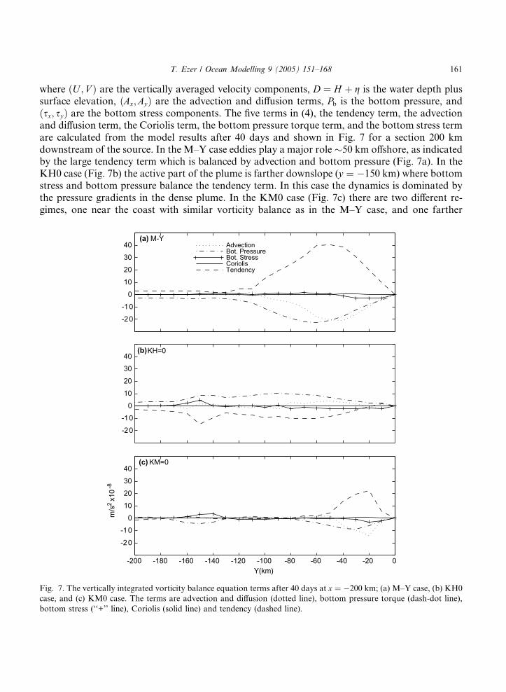
T. Ezer / Ocean Modelling 9 (2005) 151–168 161
where ðU ; V Þ are the vertically averaged velocity components, D ¼ H þ g is the water depth plussurface elevation, ðAx;AyÞ are the advection and diffusion terms, Pb is the bottom pressure, andðsx; syÞ are the bottom stress components. The five terms in (4), the tendency term, the advectionand diffusion term, the Coriolis term, the bottom pressure torque term, and the bottom stress termare calculated from the model results after 40 days and shown in Fig. 7 for a section 200 kmdownstream of the source. In the M–Y case eddies play a major role �50 km offshore, as indicatedby the large tendency term which is balanced by advection and bottom pressure (Fig. 7a). In theKH0 case (Fig. 7b) the active part of the plume is farther downslope (y ¼ �150 km) where bottomstress and bottom pressure balance the tendency term. In this case the dynamics is dominated bythe pressure gradients in the dense plume. In the KM0 case (Fig. 7c) there are two different re-gimes, one near the coast with similar vorticity balance as in the M–Y case, and one farther
-20-10
010203040
m/s
2x1
0-8
(a)
(b)
M-YAdvectionBot. PressureBot. StressCoriolisTendency
-20-10
010203040
KH=0
-200 -180 -160 -140 -120 -100 -80 -60 -40 -20 0
-20-10
010203040
Y(km)
(c) KM=0
Fig. 7. The vertically integrated vorticity balance equation terms after 40 days at x ¼ �200 km; (a) M–Y case, (b) KH0
case, and (c) KM0 case. The terms are advection and diffusion (dotted line), bottom pressure torque (dash-dot line),
bottom stress (‘‘+’’ line), Coriolis (solid line) and tendency (dashed line).
162 T. Ezer / Ocean Modelling 9 (2005) 151–168
downstream at the edge of the plume where bottom stress and bottom pressure are the dominantterms. There are no significant vorticity terms between 60 and 130 km downslope, wherehomogeneous fluid is propagating in a constant speed along the isobaths (Fig. 4c).
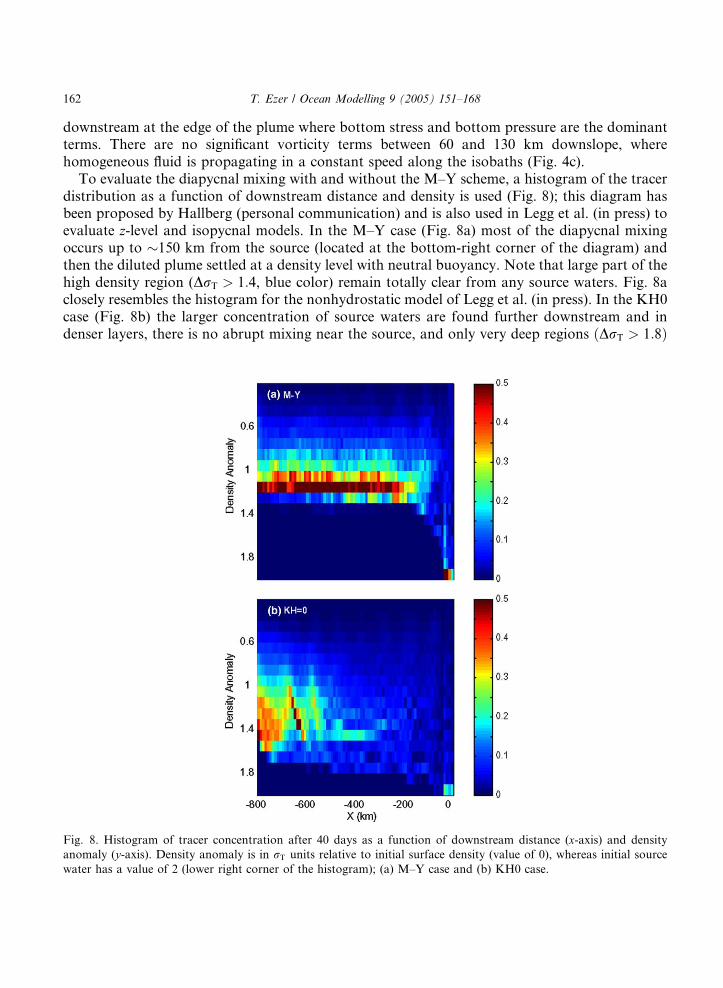
To evaluate the diapycnal mixing with and without the M–Y scheme, a histogram of the tracerdistribution as a function of downstream distance and density is used (Fig. 8); this diagram hasbeen proposed by Hallberg (personal communication) and is also used in Legg et al. (in press) toevaluate z-level and isopycnal models. In the M–Y case (Fig. 8a) most of the diapycnal mixingoccurs up to �150 km from the source (located at the bottom-right corner of the diagram) andthen the diluted plume settled at a density level with neutral buoyancy. Note that large part of thehigh density region (DrT > 1:4, blue color) remain totally clear from any source waters. Fig. 8aclosely resembles the histogram for the nonhydrostatic model of Legg et al. (in press). In the KH0case (Fig. 8b) the larger concentration of source waters are found further downstream and indenser layers, there is no abrupt mixing near the source, and only very deep regions ðDrT > 1:8Þ
Fig. 8. Histogram of tracer concentration after 40 days as a function of downstream distance (x-axis) and density
anomaly (y-axis). Density anomaly is in rT units relative to initial surface density (value of 0), whereas initial source
water has a value of 2 (lower right corner of the histogram); (a) M–Y case and (b) KH0 case.

T. Ezer / Ocean Modelling 9 (2005) 151–168 163
remain without any trace of source waters. Fig. 8b resembles results of the Hallberg IsopycnalModel (HIM) used in Legg et al. (in press).
As the plume propagating away from the source and entrained with overlaying waters, itsvolume and transport may change. This can be described by a simple mass balance equation,
Fig. 9
(dashe
show
for th
o
ox
ZAUdA ¼
ILWE; ð5Þ
where the left-hand side is the change in transport across a section A and the right-hand side is thetotal entrainment, integrating the entrainment velocity along the plume’s edge. Defining theplume in the model by tracer concentration values greater than 0.01, the plume’s downstreamtransport for the M–Y and for the KH0 cases after 40 days are shown in Fig. 9. In the M–Y casethe transport increases from the imposed 5 Sv at the embayment to about 15 Sv at x ¼ �100 km,indicating a strong diapycnal mixing (i.e., Fig. 8) and thus large entrainment (i.e., Eq. (5)) thatincreases the plume’s volume. Further downstream the transport generally decreases (i.e.,detrainment occurs). However, the oscillatory transport variation with a wavelength of �100 kmindicate small entrainment/detrainment associated with meandering and eddies. Observationsmay also indicate the possibility of some reduced transport, and thus some detrainment, fordistances over 200 km from the source (Fig. 11 in Girton and Sanford, 2003). In the KH0 case onthe other hand, the transport continues to increase, possibly indefinitely, but at least all the way tothe western boundary at x ¼ �800 km.
To summarize the distribution of the water mass that originated from the dense water overflowsource, the zonally averaged (over the model east–west domain length, X ) and vertically inte-grated tracer concentration is calculated by
CðyÞ ¼ 1
X
Zx
Zzcðx; y; zÞdxdz; ð6Þ
. Downstream plume transport as a function of x for the control run (M–Y case, solid line) and for the KH0 case
d line). The average slopes of the lines after the initial mixing (for )700 km< x < �100 km) are indicated; they
a decrease in plume transport (i.e., detrainment) for the M–Y case, but an increase in transport (i.e., entrainment)
e KH0 case.

Fig. 10. Zonal mean and vertically integrated tracer, C, as a function of downslope distance. Solid line is for the M–Y
case, dash line is for the KH0 case and dash-dot line is for the KM0 case. Also indicated by arrows are the locations of
the maxima for the POMgcs z-level case of Fig. 2e (‘‘ZLV max’’) which is similar to the KM0 case and for results from
the Hallberg Isopycnal Model, HIM (‘‘ISOPYC max’’) which is similar to the KH0 case.
164 T. Ezer / Ocean Modelling 9 (2005) 151–168
and shown for day 40 in Fig. 10. C has units of meter and is proportional to the average thicknessof the plume in the water column. In the M–Y control case the average plume thickness increasesrapidly in the first 50 km and then gradually decreases until about 250 km downslope (see alsoFig. 5a). The shape of the integrated tracer is opposite in the KH0 case, with gradual increase untilalmost 200 km downslope and then an abrupt decrease, the latter is the result of the sharp frontseen in Fig. 4b. In the KM0 case, the amount of tracer has its maximum near the northern wall(see also Fig. 5c) and gradually decreases downslope. The difference between the M–Y and theKM0 cases (most visible between y ¼ �25 and y ¼ �150 km) represents the contribution of theBBL Ekman velocity to the downslope transport of source waters; the difference is maximum atabout 100 km downslope where the Ekman transport accounts for �30% of the total accumulatedtracer. It is interesting to note that the tracer distribution in the KM0 case is somewhat similar tothat of the z-level model of Fig. 4e (the location of the maximum in the z-level calculation ismarked in Fig. 10 by ‘‘ZLV max’’; the full structure is shown in Ezer and Mellor, 2004). Thisresult supports the notion that the downslope Ekman transport is not well represented in z-levelmodels with stepped topography (without special BBL schemes), as indicated by other studies(Winton et al., 1998; Pacanowski and Gnanadesikan, 1998; Ezer and Mellor, 2004). On the otherhand, the tracer distribution in the case with no diapycnal mixing (KH0) is almost identical in itsshape to DOME experiments done with an isopycnal model (HIM, the maximum of which ismarked in Fig. 10 by ‘‘ISOPYC max’’).
4. Discussion and conclusions
Recent studies of dense gravity currents associated with overflows from observations (Girtonand Sanford, 2003) models (Jungclaus et al., 2001; Ozgokmen and Chassignet, 2002; Papadakis

T. Ezer / Ocean Modelling 9 (2005) 151–168 165
et al., 2002; K€ase et al., 2003; Ezer and Mellor, 2004; Legg et al., in press) and laboratoryexperiments (Cenedese et al., 2004), all indicate the complicated nature of the flow and the need tobetter understand the mixing processes involved. To improve simulations of overflows and deepocean formation in climate models there is a need for better parameterization of diapycnal mixingand bottom boundary layers (Griffies et al., 2000). This study is a follow-up on the model in-tercomparison study of Ezer and Mellor (2004), who compared overflow simulations in terrain-following and in z-level grids using the generalized coordinate ocean model of Mellor et al. (2002).The focus of this study is on the role played by the Mellor–Yamada (M–Y) turbulence schemewhen used in terrain-following ocean models, in determining the diapycnal mixing and the gravitycurrent transport properties. An idealized overflow configuration (Dynamics of Overflow Mixingand Entrainment setting, DOME), is used by different groups (Ezer and Mellor, 2004; Legg et al.,in press) to allow comparisons of different models and test different parameter-space regimes.
The dense plume in the DOME configuration is set with inflow velocity and plume thicknesssuch that the Froude number is subcritical ðFr6 1Þ, and thus in an eddy regime as in laboratoryexperiments (Cenedese et al., 2004) and in the Denmark Straits overflow (Jungclaus et al., 2001).This makes the representation of the overflow in coarse resolution models more difficult.Therefore, overflow simulations with z-level and terrain-following grids at 10 and 2.5 km reso-lutions are compared with results from a nonhydrostatic model with 0.5 km resolution (Legget al., in press). The nonhydrostatic model provides some ‘‘model truth’’ for this idealized case(though the resolution is still marginal for full nonhydrostatic dynamics). The comparisonsindicate too strong diapycnal mixing and not enough downslope transport in a z-level grid, whichis a well known problem (Winton et al., 1998; Ezer and Mellor, 2004), unless the steppedtopography is replaced by partial cells or special BBL schemes are added. However, a new findingis the great similarity between the results of a hydrostatic model with a terrain-following grid andthe results of a very high resolution nonhydrostatic model. While only at 2.5 km resolution thedetails of the eddies shape are well simulated, even at 10 km resolution the extent of the bottomplume, its transport and its dilution match extremely well the nonhydrostatic results. This indi-cates that the subgrid-scale parameterization of turbulent mixing, obtained here from the M–Yturbulence scheme, is doing a decent job in two aspects: 1. the space and time-dependent verticalmixing coefficient for tracers, KH, represents quite accurately the diapycnal mixing and entrain-ment of the plume, and 2. the vertical mixing coefficient for momentum, KM, represents quiteaccurately the downslope bottom Ekman transport contribution to the plume’s total transport.Special experiments with either KH ¼ 0 or KH ¼ 0 isolate the M–Y influence and reveal interestingresults. With no diapycnal mixing the plume in the terrain-following model closely resemblesresults from isopycnal models where the dense plume is driven by pressure gradients and slidesfarther downstream, with increasing transport. On the other hand, the results of the terrain-following model with reduced Ekman transport resemble results of a z-level model with steppedtopography, where large part of the dense plume remains upslope and only propagated alongisobaths. Although a simple z-level model with enough vertical resolution and a reasonable mixingcoefficient will produce horizontal bottom Ekman transport, the cross isobaths velocity compo-nent is not directly translated into a downslope transport of the dense water, but requires verticalmixing (or other convective adjustment or BBL formulation) which may dilute the plume andcreates excess diapycnal mixing. The M–Y turbulence scheme when used with a terrain-followinggrid seems to provide a reasonable compromise between the two extreme cases of a z-level like

166 T. Ezer / Ocean Modelling 9 (2005) 151–168
solution with too much diapycnal mixing and an isopycnic-like solution with too little diapycnalmixing.
Although the DOME configuration is highly idealized and primarily intends to test variousmodels and parameterizations, some of the basic observed characteristics of the Denmark Straitplume in Girton and Sanford (2003) are simulated quite well with the terrain-following model.The maximum velocity in the bottom layer range from 0.2 to 1.4 m s�1 in the model and in theobservations, the along-isobath velocity component in the model is proportional to the densityanomaly and to the slope divided by the Coriolis parameter, similar to the translation of denseeddies on a sloping bottom (Nof, 1983), and as measured in laboratory experiments of overflows(Cenedese et al., 2004). The average plume thickness is about 240 m in the model and 40–400 m inthe observations. In the model, the plume descents downslope by about 1000 m within 200 kmfrom the source, only slightly less than the observed descent, with strong entrainment near thesource that dilutes the plume and increases the plume transport. In the model, the transporttripled within the first 100 km from the source and then gradually decreases for the next 700 kmdownstream, indicating possible detrainment far from the source. Estimating the plume transportfrom cruise sections and current meter arrays shows large uncertainty (Fig. 11 in Girton andSanford, 2003), but at 150 km from the source the observed transport seems to be 2–3 times thesource transport, and there is some indication for reduced transport farther than 150 km from thesource, as seen in the model. Combining the results of various idealized and realistic models withnew observations of overflows will eventually lead to better parameterization of such flows inocean models, and better understanding of their dynamics.
Acknowledgements
This study is part of the Climate Process Team-Gravity Current Entrainment (CPT-GCE)project, supported by NSF award # OCE-0336768. All the CPT team members are thanked formany useful discussions, and in particular Sonya Legg and Bob Hallberg who provided resultsfrom the MIT and HIM models prior to publication which were essential for the comparison withthe terrain-following model. Additional support is provided by the Office of Naval Research(ONR), award # N00014-04-10381. Comments by George Mellor and two anonymous reviewerswere helpful to improve the manuscript. Computational resources were provided by the High-Performance Computing System (HPCS) at NOAA’s Geophysical Fluid Dynamics Laboratory(GFDL).
References
Adcroft, A., Hill, C., Marshall, J., 1997. Representation of topography by shaved cells in a height coordinate ocean
model. Monthly Weather Review 125, 2293–2315.
Beckmann, A., D€oscher, R., 1997. A method for improved representation of dense water spreading over topography in
geopotential-coordinate models. Journal of Physical Oceanography 27, 581–591.
Blumberg, A.F., Mellor, G.L., 1987. A description of a three-dimensional coastal ocean circulation model. In: Heaps,
N.S. (Ed.), Three-Dimensional Coastal Ocean Models. In: Coastal Estuarine Studies, vol. 4. American Geophysical
Union, Washington, DC, pp. 1–16.
T. Ezer / Ocean Modelling 9 (2005) 151–168 167
Campin, J.-M., Goosse, H., 1999. Parameterization of density-driven downsloping flow for a coarse-resolution ocean
model in z-coordinate. Tellus 51A, 412–430.
Cenedese, C., Whitehead, J.A., Ascarelli, T.A., Ohiwa, M., 2004. A dense current flowing down a sloping bottom in a
rotating fluid. Journal of Physical Oceanography 34, 188–203.
Ezer, T., 2000. On the seasonal mixed-layer simulated by a basin-scale ocean model and the Mellor–Yamada turbulence
scheme. Journal of Geophysical Research 105, 16,843–16,855.
Ezer, T., Arango, H., Shchepetkin, A.F., 2002. Developments in terrain-following ocean models: Intercomparisons of
numerical aspects. Ocean Modelling 4, 249–267.
Ezer, T., Mellor, G.L., 2004. A generalized coordinate ocean model and a comparison of the bottom boundary layer
dynamics in terrain-following and in z-level grids. Ocean Modelling 6, 379–403.
Ezer, T., Weatherly, G.L., 1990. A numerical study of the interaction between a deep cold jet and the bottom boundary
layer of the ocean. Journal of Physical Oceanography 20, 801–816.
Gerdes, R., 1993. A primitive equation ocean circulation model using a general vertical coordinate transformation. 1.
Description and testing of the model. Journal of Geophysical Research 98, 14,683–14,701.
Girton, J.B., Sanford, T.B., 2003. Descent and modification of the overflow plume in the Denmark Strait. Journal of
Physical Oceanography 33, 1351–1364.
Griffies, S.M., Boning, C., Bryan, F.O., Chassignet, E.P., Gerdes, R., Hasumi, H., Hirst, A., Treguier, A., Webb, D.,
2000. Developments in ocean climate modelling. Ocean Modelling 2, 123–192.
Haidvogel, D.B., Arango, H., Hedstrom, K., Beckmann, A., Malanotte-Rizzoli, P., Shchepetkin, A.F., 2000. Model
evaluation experiments in the North Atlantic basin: Simulations in nonlinear terrain-following coordinates.
Dynamics of Atmospheres and Oceans 32, 239–282.
Hallberg, R.W., 2000. Time integration of diapycnal diffusion and Richardson number dependent mixing in isopycnal
coordinate ocean models. Monthly Weather Review 128, 1402–1419.
Jiang, L., Garwood Jr., R.W., 1996. Three-dimensional simulations of overflows on continental slopes. Journal of
Physical Oceanography 26, 1214–1233.
Jungclaus, J.H., Mellor, G.L., 2000. A three-dimensional model study of the Mediterranean outflow. Journal of Marine
Systems 24, 41–66.
Jungclaus, J.H., Hauser, J., K€ase, R.H., 2001. Cyclogenesis in the Denmark Strait overflow plume. Journal of Physical
Oceanography 31, 3214–3229.
K€ase, R.H., Girton, J.B., Sanford, T.B., 2003. Structure and variability of the Denmark Strait overflow: Model and
observations. Journal of Geophysical Research 108 (C6), doi: 10.1029/2002JC001548.
Killworth, P.D., Edwards, N.R., 1999. A turbulent bottom boundary layer code for use in numerical models. Journal of
Physical Oceanography 29, 1221–1238.
Legg, S., Hallberg, R.W., Girton, J.B., in press. Comparison of entrainment in overflows simulated by z-coordinate,isopycnal and nonhydrostatic models. Ocean Modelling.
Marshall, J., Jones, H., Hill, C., 1998. Efficient ocean modeling using nonhydrostatic algorithms. Journal of Marine
Systems 18, 115–134.
Martin, P.J., 1985. Simulation of the mixed layer at OWS November and papa with several models. Journal of
Geophysical Research 90, 903–916.
Mellor, G.L., Yamada, T., 1982. Development of a turbulent closure model for geophysical fluid problems. Review of
Geophysics 20, 851–875.
Mellor, G.L., Hakkinen, S., Ezer, T., Patchen, R., 2002. A generalization of a sigma coordinate ocean model and an
intercomparison of model vertical grids. In: Pinardi, N., Woods, J.D. (Eds.), Ocean Forecasting: Conceptual Basis
and Applications. Springer, pp. 55–72.
Nof, D., 1983. The translation of isolated cold eddies on a sloping bottom. Deep-Sea Research 30, 171–182.
Ozgokmen, T.M., Chassignet, E., 2002. Dynamics of two-dimensional turbulent bottom gravity currents. Journal of
Physical Oceanography 32, 1460–1478.
Pacanowski, R.C., Gnanadesikan, A., 1998. Transient response in a z-level ocean model that resolves topography with
partial cells. Monthly Weather Review 126, 3248–3270.
Papadakis, M.P., Chassignet, E.P., Hallberg, R.W., 2002. Numerical simulations of the Mediterranean sea outflow:
Impact of the entrainment parameterization in an isopycnic coordinate ocean model. Ocean Modeling 5, 325–356.
168 T. Ezer / Ocean Modelling 9 (2005) 151–168
Price, J.F., Barringer, M.O., 1994. Outflows and deep water production by marginal seas. Progress in Oceanography 33,
161–200.
Song, Y.T., Chao, Y., 2000. An embedded bottom boundary layer formulation for z-coordinate ocean models. Journal
of Atmospheric and Oceanic Technology 17, 546–560.
Song, Y.T., Haidvogel, D., 1994. A semi-implicit ocean circulation model using a generalized topography following
coordinate system. Journal of Computational Physics 115, 228–248.
Warner, J.C., Sherwood, C.R., Arango, H.G., Signell, R.P., in press. Performance of four turbulence closure models
implemented using a generic length scale method. Ocean Modelling 7.
Winton, M., Hallberg, R.W., Gnanadesikan, A., 1998. Simulation of density-driven frictional downslope flow in
z-coordinate ocean models. Journal of Physical Oceanography 28, 2163–2174.