ensemble missing data techniques for software effort
TRANSCRIPT

Intelligent Data Analysis 14 (2010) 299–331 299DOI 10.3233/IDA-2010-0423IOS Press
Ensemble missing data techniques forsoftware effort prediction
Bhekisipho Twalaa,∗ and Michelle CartwrightbaDepartment of Electrical and Electronic Engineering Science, University of Johannesburg, P.O. Box524, Auckland Park, Johannesburg 2006, South AfricabBrunel Software Engineering Research Centre, School of Information Systems, Computing andMathematics, Brunel University, Uxbridge, UK
Abstract. Constructing an accurate effort prediction model is a challenge in software engineering. The development andvalidation of models that are used for prediction tasks require good quality data. Unfortunately, software engineering datasets tendto suffer from the incompleteness which could result to inaccurate decision making and project management and implementation.Recently, the use of machine learning algorithms has proven to be of great practical value in solving a variety of softwareengineering problems including software prediction, including the use of ensemble (combining) classifiers. Research indicatesthat ensemble individual classifiers lead to a significant improvement in classification performance by having them vote for themost popular class. This paper proposes a method for improving software effort prediction accuracy produced by a decisiontree learning algorithm and by generating the ensemble using two imputation methods as elements. Benchmarking results onten industrial datasets show that the proposed ensemble strategy has the potential to improve prediction accuracy compared toan individual imputation method, especially if multiple imputation is a component of the ensemble.
Keywords: Machine learning, supervised learning, decision tree, software prediction, incomplete data, imputation, missing datatechniques, ensemble
Abbreviations
CART: Classification and Regression TreesCCCS: Command, Control and Communications SystemCMI: Class Mean ImputationDA: Data AugmentationDSI: Defence Security InstituteDT: Decision TreeDTSI: Decision Tree Single ImputationEM: Expectation-MaximizationEMSI: Expectation-maximization Single ImputationFC: Fractioning of CasesFIML: Full Information Maximum LikelihoodHDSI: Hot-Deck Single ImputationISBSG: International Software Benchmarking Standards Group
∗Corresponding author: Bhekisipho Twala, Department of Electrical and Electronic Engineering Science, University ofJohannesburg, P.O. Box 524, Auckland Park, Johannesburg 2006, South Africa. Tel.: +27 11 559 4404; Fax: +27 11 559 2357;E-mail: [email protected].
1088-467X/10/$27.50 2010 – IOS Press and the authors. All rights reserved

300 B. Twala and M. Cartwright / Ensemble missing data techniques for software effort prediction
IM: Informatively Missingk-NN: k-Nearest Neighbourk-NNSI: k-Nearest Neighbour Single ImputationLD: Listwise DeletionMAR: Missing at RandomMCAR: Missing Completely at RandomMDT: Missing Data TechniqueMI: Multiple ImputationMIA: Missingness Incorporated in AttributesML: Machine LearningMMSI: Mean or Mode Single ImputationRBSI: Regression-Based Single ImputationRPART: Recursive Partitioning and Regression TreesSE: Software EngineeringSL: Supervised LearningSMI: Sample Mean ImputationSRPI: Similar Response Pattern ImputationSVS: Surrogate Variable Splitting
1. Introduction
Software engineering (SE) researchers and practitioners remain concerned with prediction accuracywhen building prediction systems. Lack of adequate tools to evaluate and estimate the cost for a softwareproject is one of the main challenges in SE. We use datasets of past projects to build and validateestimation or prediction systems of software development effort, for example, which allows us to makemanagement decisions, such as resource allocation. Or we may use datasets of measurements describingsoftware systems to validate metrics predicting quality attributes.
Various ML techniques have been used in SE to predict software cost [5], software (project) devel-opment effort [6,26,61], software quality [17], and software defects [18,45]. Reviews of the use of MLin SE [37,38] report that ML in SE is a mature technique based on widely-available tools using wellunderstood algorithms. The decision tree (DT) classifier is an example of a ML algorithm that canbe used for predicting continuous attributes (regression) or categorical attributes (classification). Thus,software prediction can be cast as a supervised learning (SL) problem, i.e., the process of learning toseparate samples from different classes by finding common features between samples of known classes.An important advantage of ML over statistical analysis as a modelling technique lies in the fact that theinterpretation of, say, decision rules is more straightforward and intelligible to human beings than, say,principal component analysis (a statistical tool for finding patterns in data of high dimension). In recentyears, there has been an explosion of papers in the ML and statistics communities discussing how tocombine models or model predictions.
Most techniques for predicting attributes of a software system or project data require past data fromwhich models will be constructed and validated. An important and common issue faced by researcherswho use industrial and research datasets is incompleteness of data. Even if part of a well thought outmeasurement programme, industrial datasets can be incomplete, for a number of reasons. These includeinaccurate or non reporting of information (without a direct benefit, a project manager or developermight see data collection as an overhead they can ill afford, for example), or, where data from a number

B. Twala and M. Cartwright / Ensemble missing data techniques for software effort prediction 301
of different types of projects or from a number of companies are combined, certain fields may be blankbecause they are not collectable for all projects. Often data is collected either with no specific purposein mind (i.e. it is collected because it might be useful in future) or the analysis being carried out has adifferent goal than that for which the data was originally collected. In research datasets, e.g. experimentson human subjects to assess the effectiveness of a new SE technique, say, dropout or failure to followinstructions may lead to missing values. The relevance of this issue is strictly proportional to thedimensionality of the collected data. SE researchers have become increasingly aware of the problemsand biases which can be caused by missing or incomplete data. Moreover, many SE datasets tend tobe small with many different attributes – software project datasets grow slowly, for example – and thenumbers of available human subjects limit the size of many experimental datasets. Thus, we can illafford to reduce our sample size further.
Many works in both the ML and statistical pattern recognition communities have shown that combining(ensemble) individual classifiers is an effective technique for improving classification accuracy. Anensemble is generated by training multiple learners for the same task and then combining their predictions.There are different ways in which ensembles can be generated, and the resulting output combined toclassify new instances. The popular approaches to creating ensembles include changing the instancesused for training through techniques such as bagging [1,4], boosting [19], changing the features used intraining [21], and introducing randomness in the classifier itself [13]. The interpretability of classifierscan produce useful information for experts responsible for making reliable classification decisions,making DTs an attractive scheme.
There are various reasons why DTs and not other SL algorithms were utilized to investigate theproblem considered in this paper. Despite being one of the well known algorithms from the ML andstatistical pattern recognition communities, DTs are non-parametric and are relatively fast to construct;classification is very fast too. They work for almost all classification problems and can achieve goodperformance on many tasks. However, one property that sets DTs apart from all other ML methodsis their invariance to monotone transformations of the predictor variables. For example, replacing anysubset of the predictor variables {xj} by (possible different) arbitrary strictly monotone functions ofthem {xj ← mj(xj)}, gives rise to the same tree model. Thus, there is no issue of having to experimentwith different possible transformations mj(xj) for each individual predictor xj to try to find the bestones. This invariance provides immunity to the presence of extreme values (“outliers”) in the predictorvariable space. In addition, DTs incorporate a pruning scheme that partially addresses the outlier (noise)removal problem. DTs also make good candidates for combining because they are structurally unstableclassifiers and produce diversity in classifier decision boundaries. DTs have also been one of the toolsof choice for building classification models in the SE field [29,30,46–48,58,64–66,70–72]. We assumethat the readers are familiar with DT learning [4,49]. However, a brief introduction on DTs is given inSection 3.
To the best of our knowledge, our research group was the first to present the effect of ensemble missingdata techniques (MDTs) on predictive accuracy in the SE field [70,72]. In this paper, we expand on thepreliminary work by first assessing the robustness of eight MDTs on the predictive accuracy of resultingDTs. We then propose three ensemble methods with each ensemble having two MDTs as elements. Theproposed method utilizes probability patterns of classification results.
The following section briefly discusses missing data patterns and mechanisms that lead to the introduc-tion of missing values in datasets. Section 3 gives a brief introduction on DTs, followed by a presentationof techniques that have been used to handle incomplete data when using DTs. The proposed ensembleprocedure is also described. Section 5 reviews some related work to the problem of incomplete data in

302 B. Twala and M. Cartwright / Ensemble missing data techniques for software effort prediction
the SE area. Section 6 empirically explores the robustness and accuracy of eight MDTs to ten industrialdatasets. This section also presents empirical results from the application of the proposed ensembleprocedure with current MDTs. We close with conclusions and directions for future research.
2. Patterns and mechanisms of missing data
The two other crucial tasks when dealing with incomplete data are to investigate the pattern of missingdata and the mechanism underlying the missingness. This is to get an idea of the process that could havegenerated the missing data, and to produce sound estimates of the parameters of interest, despite the factthat the data are incomplete.
The pattern simply defines which values in the data set are observed and which are missing. Thethree most common patterns of non-response in data are univariate, monotonic and arbitrary. Whenmissing values are confined to a single variable we have a univariate pattern; monotonic pattern occursif a subject, say Yj , is missing then the other variables, say Yj+1,. . . Yp, are missing as well or whenthe data matrix can be divided into observed and missing parts with a “staircase” line dividing them;arbitrary patterns occur when any set of variables may be missing for any unit.
The law generating the missing values seems to be the most important task since it facilitates how themissing values could be estimated more efficiently. If data are missing completely at random (MCAR)or missing at random (MAR), we say that missingness is ignorable. In other words, the analyst canignore the missing data mechanism provided the values are MCAR or MAR. For example, suppose thatyou are modelling software defects as a function of development time. If missingness is not related tothe missing values of defect rate itself and also not related on the values of development time, such datais considered to be MCAR. For example, there may be no particular reason why some project managerstold you their defect rates and others did not.
Secondly, software defects may not be identified or detected due to a given specific development time.Such data are considered to be MAR. MAR essentially says that the cause of missing data (softwaredefects) may be dependent on the observed data (development time) but must be independent of themissing value that would have been observed. It is a less restrictive model than MCAR, which says thatthe missing data cannot be dependent on either the observed or the missing data. MAR is also a morerealistic assumption for data to meet, but not always tenable. The more relevant and related attributesone can include in statistical models, the more likely it is that the MAR assumption will be met.
Finally, for data that is informatively missing (IM) or not missing at random (NMAR) then themechanism is not only non-random and not predictable from the other variables in the dataset but cannotbe ignored, i.e., we have non ignorable missingness [36,55]. In contrast to the MAR condition outlinedabove, IM arise when the probability that defect rate is missing depends on the unobserved value ofdefect rate itself. For example, software project managers may be less likely to reveal projects with highdefect rates. Since the pattern of IM data is not random, it is not amenable to common MDTs and thereare no statistical means to alleviate the problem.
MCAR is the most restrictive of the three conditions and in practice it is usually difficult to meet theMCAR assumption. Generally you can test whether MCAR conditions can be met by comparing thedistribution of the observed data between the respondents and non-respondents. In other words, datacan provide evidence against MCAR. However, data cannot generally distinguish between MAR andIM without distributional assumptions, unless the mechanisms is well understood. For example, rightcensoring (or suspensions) is IM but is in some sense known. An item or unit, which is removed from areliability test prior to failure or a unit which is in the field and is still operating at the time the reliabilityof these units is to be determined is called a suspended item or right censored instance.

B. Twala and M. Cartwright / Ensemble missing data techniques for software effort prediction 303
Table 1Attribute variables and values
Attribute Possible valuesAdjusted function points (ADJFPs) continuousDuration in months (DUR) continuousExperience of project manager in years (EXPPM) continuousNumber of transactions (TRANS) continuousSkill level of development team (SKILL) beginner, intermediate, advanced
3. Decision trees
DT induction is one of the simplest and yet most successful forms of SL algorithm. It has beenextensively pursued and studied in many areas such as statistics [4] and machine learning [49–51] forthe purposes of classification and prediction.
DT classifiers have four major objectives. According to Safavian and Landgrebe [53], these are: 1) toclassify correctly as much of the training sample as possible; 2) generalise beyond the training sample sothat unseen samples could be classified with as high accuracy as possible; 3) be easy to update as moretraining samples become available (i.e., be incremental; 4) and have as simple a structure as possible.Objective 1) is actually highly debatable and to some extent conflicts with objective 2). Also, not all treeclassifiers are concerned with objective 3).
DTs are non-parametric (no assumptions about the data are made) and a useful means of representingthe logic embodied in software routines. A DT takes as input a case or example described by a set ofattribute values, and outputs a Boolean or multi-valued “decision”. For the purpose of this paper, weshall stick to the Boolean case (thus, binary DTs) for several reasons given below.
The power of the Boolean approach comes from its ability to split the instance space into subspaceswhere each subspace is fitted with different models. Other distinctive advantages of Boolean expressionsare their time complexity and space complexity, i.e., as the input size as Boolean functions grow linearly,computer time and storage requirements of algorithms to represent and manipulate DTs do not necessarilygrow exponentially (as is the case for traditional representation techniques). Thus, both the memoryspace to store DT and the time of the learning and using phase are decreased [41]. Furthermore,information-based attribute selection measures used in the induction of DTs are all biased in favour ofattributes that have many possible values [74].
The use of Boolean attributes is one strategy for handling multi-valued attributes and as a resultovercomes this problem, i.e., attributes with fewer levels and those with many levels are all selected ona competitive basis.
Consider the following fictitious SE example, where the categorical attribute specifies whether a projectis likely to require low, medium or high software effort (EFFORT) based on attributes related to softwaredevelopment. The attributes are summarized in Table 1.
The training data is used to build the model or classifier (a DT) and a corresponding hierarchicalpartitioning shown in Figs 1 (a) and 1 (b), respectively. The DT has classes low, medium and high. Thisis a classifier in the form of a tree, a structure that is either: a leaf (rectangular box), indicating a class,or a decision node (ovals) that specifies some test to be carried out on a single attribute value, with onebranch and sub-tree for each possible outcome of the test. Notice that Test 1, Test 2 and Test 3 are testson the real-valued attributes. Only test 4 uses the nominal attribute. Further note that the attribute DURhas been not utilised in the DT even though we have it as one of the continuous attributes in the trainingdata. It is also easy to see that as the depth of the tree increases, the resulting partitioning becomes moreand more complex.

304 B. Twala and M. Cartwright / Ensemble missing data techniques for software effort prediction
(a)
(b)
Fig. 1. (a) Example of a binary axis-parallel decision tree for a four-dimensional feature space and 3 classes for decidingthe likely level of effort for a project. Ovals represent internal nodes; rectangles represent leaf nodes or terminal nodes. (b)Hierarchical partitioning of the two-dimensional feature space induced by the decision tree of Fig. 1(a)
The prediction problem is handled by partitioning classifiers. These classifiers split the space ofpossible observations into partitions. For example, when a project manager needs to make a decisionwhether a project is likely to require low, medium of high effort based on several software developmentfactors, a classification tree can help identify which factors to consider and how each factor has historicallybeen associated with different outcomes of the decision.
4. Decision trees and missing data
Several methods have been proposed in the literature to treat missing attribute values (incomplete data)when using DTs. Missing values can cause problems at two points when using DTs; 1) when deciding ona splitting point (when growing the tree), and 2) when deciding into which daughter node each instancegoes (when classifying an unknown instance). Methods for taking advantage of unlabelled classes can

B. Twala and M. Cartwright / Ensemble missing data techniques for software effort prediction 305
Table 2Missing data techniques
Techniques SectionDiscarding data: 4.1
Listwise deletion 4.1Imputation: 4.2
Single Imputation 4.2.1mean or mode 4.2.1.1k-nearest neighbour 4.2.1.2decision tree* 4.2.1.3
Missing Incorporated in Attributes 4.2.2Multiple Imputation 4.2.3Supervised Learning Imputation 4.2.4
surrogate variable splitting 4.2.4.1fractioning of cases 4.2.4.2
Ensembles 4.3
* Also a supervised learning algorithm.
also be developed, although we do not deal with them in this paper, i.e., we are assuming that the classlabels are not missing.
Specific DT techniques for handling incomplete data are now going to be discussed. These missingdata techniques (MDTs) are some of the widely recognized and they are divided into three categories:ignoring and discarding data, imputation and SL or ML. The MDTs are briefly described in the followingsections and summarized in Table 2.
4.1. Ignoring and discarding data (Listwise deletion)
Incomplete data are often dealt with by using several general approaches, like, deleting the instanceswith missing data which aim to modify up the data so that they can be analysed by methods designedfor complete data. Basically, listwise deletion (LD) means that any individual with missing data onany variable is deleted from the analysis under consideration. This approach can drastically reduce thesample size since it can sacrifice a large amount of data leading to a severe lack of statistical power [36].It can even lead to complete case loss if many variables are involved. However, due to its simplicity andease of use, LD is the default in most statistical packages.
4.2. Imputation techniques
Imputation techniques fill in (impute) missing items with plausible values in the dataset, thus makingit possible to analyze the data as if it were complete. Two kinds of imputation strategies are discussedin this paper: single imputation (SI) and multiple imputation (MI). SI refers to filling in a missing valuewith a single replacement value while multiple values are simulated for MI. A brief description of eachimputation method is given below.
4.2.1. Single imputation4.2.1.1. Mean or mode imputation
Some researchers have used arbitrary methods like mean imputation for addressing the missing valueproblem, i.e., replacing the missing values of a variable by the mean of its observed values. Meansubstitution also assumes a MCAR mechanism. The strength of mean imputation is that it preservesthe data and it is easy to use. However, mean imputation can be misleading because it produces biased

306 B. Twala and M. Cartwright / Ensemble missing data techniques for software effort prediction
and inconsistent estimates of both coefficients and standard errors). Little and Rubin [36] point out thatvariance parameter estimates under mean imputation are generally negatively biased. Also, substitutionof the simple (grand) mean will reduce the variance of the variable and its correlation with other variables.Somewhat better is substitution of the group or global mean (or mode in the case of nominal data) for agrouping variable known to correlate as highly as possible with the variable which has missing values.We shall now call this technique mean or mode single imputation (MMSI).
4.2.1.2. k-nearest neighbour imputationWe use the k-nearest neighbour (k-NN) approach to determine the imputed data, where nearest is
usually defined in terms of a distance function based on the auxiliary variable(s). In this method a poolof complete instances is found for each incomplete instance and the imputed values for each missingcell in each recipient is calculated from the values of the respective field in complete instances [10].The strength of k-NN lies in its ability to predict both discrete attributes (the most frequent value amongthe k nearest neighbours) and continuous attributes (the mean among the k nearest neighbours). Also,k-NN can be easily adapted to work with any attribute as class, by just modifying which attributes willbe considered in the distance metric. This single imputation approach, which also assumes a MCARmechanisms, shall now be called k−NNSI.
4.2.1.3. Decision tree imputationThe unordered attribute DTs approach, which can also be considered a machine learning technique
as it uses a DT algorithm to impute missing values, is another strategy that has been used for handlingmissing values in tree learning. This technique was suggested by Shapiro [60]. The method builds DTsto determine the missing values of each attribute, and then fills the missing values of each attribute byusing its corresponding tree. Separate trees are built using a reduced training set for each attribute, i.e.,restricting your analysis to only those instances that have known values. The original class is treated asanother attribute, while the value of the attribute becomes the “class” to be determined. The attributesused to grow the respective trees are unordered. These trees are then used to determine the unknownvalues of that particular attribute.
For this strategy, it is not clear what the probability generating the missingness is for both strategies.However due to the fact that the dependencies between attributes is not considered, we shall assume thatthe data is MCAR.
4.2.2. Missingness incorporated in attributesThis approach proposed by Twala [68] and followed up by Twala et al. [69] is closely related to the
technique of treating “missing” as a category in its own right, generalizing it for use with continuous aswell as categorical variables as described below:
Let Xn be an ordered or numeric attribute variable with unknown attribute values, the proposedapproach searches essentially over all possible values of xn for binary splits of the following form:
1. Split A: (Xn � xn or Xn = missing) versus (Xn > xn)2. Split B: (Xn � xn) versus (Xn > xnor Xn = missing)3. Split C: (Xn = missing) versus (Xn = not missing)
The idea is to find the best split from the candidate set of splits given above, with the goodness of splitmeasured by how much it decreases the impurity of the sub-samples.
If Xn is a nominal attribute variable (i.e., a variable that takes values in an unordered set), the searchis over all splits of the form:

B. Twala and M. Cartwright / Ensemble missing data techniques for software effort prediction 307
1. Split A: (Xn ∈ Yn or Xn = missing) versus (Xn /∈ Yn)2. Split B: (Xn ∈ Yn) versus (Xn /∈ Yn or Xn = missing)3. Split C: (Xn = missing) versus (Xn = not missing)
where Yn is the splitting subset at node n.So, if there were ∂ options for splitting a branch without missingness, there are 2∂+ 1 options to be
explored with missingness present.This missingness incorporated in attributes (MIA) algorithm is very simple, natural and applicable to
any method of constructing DTs, regardless of that method’s detailed splitting/stopping/pruning rules. Ithas a very close antecedent: the approach of handling unknown attribute values by treating all attributesas categorical and adding missingness as a further category. The two approaches are superficially thesame but differ a little in their treatment of continuous attributes: rather than categorizing continuousvariables, missingness is directly incorporated in splits of continuous variables. The approach can beexpected to be particularly useful when missingness is not random but informative. Classifying a newindividual whose value of a branching attribute is missing is immediately provided, especially if theattribute in the training set that was used to construct the DT had missing values.
4.2.3. Multiple imputationMI is one of the most attractive methods for general purpose handling of missing data in multivariate
analysis. Rubin [52] described MI as a three-step process. First, sets of plausible values for missinginstances are created using an appropriate model that reflects the uncertainty due to the missing data.Each of these sets of plausible values can be used to “fill-in” the missing values and create a “completed”dataset. Second, each of these datasets can be analyzed using complete-data methods. Finally, theresults are combined. For example, replacing each missing value with a set of five plausible values orimputations would result to building five DTs, and the predictions of the five trees would be averagedinto a single tree, i.e., the average tree is obtained by MI.
MI retains most of the advantages of single imputation and rectifies its major disadvantages as alreadydiscussed. There are various ways to generate imputations. Schafer [55] has written a set of generalpurpose programs for MI of continuous multivariate data (NORM), multivariate categorical data (CAT),mixed categorical and continuous (MIX), and multivariate panel or clustered data (PNA). These programswere initially created as functions operating within the statistical languages S and SPLUS [73]. NORMincludes and EM algorithm for maximum likelihood estimation of means, variance and covariances.NORM also adds regression-prediction variability by a procedure known as data augmentation [55].
Although not absolutely necessary, it is almost always a good idea to run the expectation maximization(EM) algorithm [12] before attempting to generate MIs. The parameter estimates from EM provideconvenient starting values for data augmentation (DA). Moreover, the convergence behaviour of EMprovides useful information on the likely convergence behaviour of DA. In brief, EM is an iterativeprocedure where a complete dataset is created by filling-in (imputing) one or more plausible values forthe missing data by repeating the following steps: 1.) In the E-step, one reads in the data, one instanceat a time. As each case is read in, one adds to the calculation of the sufficient statistics (sums, sums ofsquares, sums of cross products). If missing values are available for the instance, they contribute to thesesums directly. If a variable is missing for the instance, then the best guess is used in place of the missingvalue. 2.) In the M-step, once all the sums have been collected, the covariance matrix can simply becalculated. This two step process continues until the change in covariance matrix from one iteration tothe next becomes trivially small. This is the approach we follow in this paper.
Details of the EM algorithm for covariance matrices are given in [12,36,55]. EM requires that dataare MAR.

308 B. Twala and M. Cartwright / Ensemble missing data techniques for software effort prediction
4.2.4. Supervised learning imputationSL techniques are those that deal with missing values using ML algorithms. ML algorithms learn
a function from training data. The training data consist of pairs of input objects (vectors) and desiredoutput. The output of the function can be a continuous value (called regression) or can predict a classlabel of the input object (called classification). ML techniques are generally more complex than statisticaltechniques. This section will describe missing data imputation using two supervised machine learningsystems: surrogate variable splitting and fractioning of cases.
4.2.4.1. Surrogate variable splittingOne sophisticated but refined method worthy of note and study is the surrogate variable splitting (SVS),
which has been used for the classification and regression trees (CART) system [4]. CART handles missingvalues in the database by substituting "surrogate splitters". Surrogate splitters are predictor variables thatare not as good at splitting a group as the primary splitter but which yield similar splitting results; theymimic the splits produced by the primary splitter; the second does second best, and so on. The surrogatesplitter contains information that is typically similar to that which would be found in the primary splitter.The surrogates are used for tree nodes when there are values missing. The surrogate splitter containsinformation that is typically similar to what would be found in the primary splitter. Both values forthe dependent variable (response) and at least one of the independent variables (attributes) take part inthe modelling. The surrogate variable used is the one that has the highest correlation with the originalattribute (observed variable most similar to the missing variable or a variable other than the optimal onethat best predicts the optimal split). The surrogates are ranked. Any observation missing on the splitvariable is then classified using the first surrogate variable, or if missing that, the second is used, and soon. The CART system only handles missing values in the testing case but RPART handles them on boththe training and testing cases.
SVS makes no assumption about the law generating the missingness. However, due to the fact that ituses the dependencies between attributes, we shall assume that the data is MAR.
4.2.4.2. Fractioning of casesQuinlan [49] borrows the probabilistic complex approach by Cestnik et al. [8] by “fractioning” cases
or instances based on a priori probability of each value determined from the cases at that node thathave specified values. Quinlan starts by penalising the information gain measure by the proportion ofunknown cases and then splits these cases to both subnodes of the tree.
The learning phase requires that the relative frequencies from the training set be observed. Eachcase of, say, class C with an unknown attribute value A is substituted. The next step is to distributethe unknown examples according to the proportion of occurrences in the known instances, treating anincomplete observation as if it falls down all subsequent nodes. The evaluation measure is weightedwith the fraction of known values to take into account that the information gained from that attribute willnot always be available (but only in those cases where the attribute value is known). During training,instance counts used to calculate the evaluation heuristic include the fractional counts of instances withmissing values. Instances with multiple missing values can be fractioned multiple times into numeroussmaller and smaller “portions”.
For classification, Quinlan’s technique is to explore all branches below the node in question and thentake into account that some branches are more probable than others. Quinlan, once again, borrowsCestnik et al.’s [8] strategy of summing the weights of the instance fragments classified in different waysat the leaf nodes of the tree and then choosing the class with the highest probability or the most probable

B. Twala and M. Cartwright / Ensemble missing data techniques for software effort prediction 309
1. Partition original dataset into n incomplete training datasets, ITR1, ITR2, , ITRn.
2. Construct n individual DT models (DT1, DT2, , DTn) with the different incomplete training
datasets ITR1, ITR2, , ITRn to obtain n individual DT classifiers (ensemble members) generated
by different imputation algorithms, thus different.
3. Select m de-correlated DT classifiers from n DTs using de-correlation maximization algorithm.
4. Using Eq. 3, obtain m DTs output values (misclassification error rates) of unknown instance.
5. Transform the output value to reliability degrees of positive class and negative class, given the
imbalance of some datasets
6. Fuse the multiple DTs into aggregate output in terms of majority voting. When there is a tie in the
predicted probabilities, choose the class with the highest probability or else use a random choice
when the probabilities between the two methods are equal.
Fig. 2. The ensemble imputation methods algorithm.
classification. Basically, when a test attribute has been selected, the cases with known values are dividedon the branches corresponding to these values. The cases with missing values are, in a way, passeddown all branches, but with a weight that corresponds to the relative frequency of the value assigned toa branch. Both strategies for handling missing attribute values are used for the C4.5 system [49].
FC does not consider the dependencies of attributes to predict missing attribute values. Thus, we shallassume that the data is MCAR.
4.3. Ensemble imputation methods
Our proposed method uses DTs as its component classifier. The main objective is to combinepredictions of this classifier. A motivation for ensemble is that a combination of outputs of many weakMDTs produces a powerful ensemble MDTs with higher accuracy than a single MDT obtained fromthe same sample. The proposed method makes use of all data available and utilises a systematic patternof classification results based on two methods for handling incomplete training and test data. The newgeneralized algorithm is summarised in Fig. 2, with the overall six-stage scheme of the technique shownin Fig. 3 and described in more detail in the following sections.
4.3.1. Partitioning original datasetDue to the shortage in some data analysis problems, such approaches, such as bagging [2] have been
used for creating samples varying the data subsets selected. The bagging algorithm is very efficient inconstructing a reasonable size of training set due to the feature of its random sampling with replacement.Therefore such a strategy (which we also use in this study) is a useful data preparation method for ML.
4.3.2. Creating diverse decision tree classifierDiversity in ensemble of learnt models constitute one of the main current directions in ML and data
mining. It has been shown theoretically and experimentally that in order for an ensemble to be effective,it should consist of high-accuracy base classifiers that should have high diversity in their predictions.One technique, which proved to be effective for constructing an ensemble of accurate and diverse baseclassifiers, is to use different training data, or so-called ensemble training data selection. Many ensemble

310 B. Twala and M. Cartwright / Ensemble missing data techniques for software effort prediction
Input
Output
DTnDT2
DT fnDT f2DT f1
fm(x)fs(x)f1(x)
gm(x)g2(x)g1(x)
F(x)
DT1
Testing Data set(TD)
Validation Data set(VD)
Original Data set(OD)
Incomplet eTraining Data set
(TRn)
Incomplet eTraining Data set
(TR2)
Incomplet eTraining Data set
(ITR1)
Incompelt eTraining Data set
(ITR)
.
Stag e 1
Stage 4
Stage 5
Stage 6
Stage 3
Stage 2
Fig. 3. The general formation process of missing data ensemble learning model.

B. Twala and M. Cartwright / Ensemble missing data techniques for software effort prediction 311
training data selection strategies generate multiple classifiers by applying a single learning algorithm, todifferent versions of a given dataset, Two different methods for manipulating the dataset are normallyused: random sampling with replacement (also called bootstrap sampling) in bagging and re-weightingof the misclassified training instances in boosting. In our study, bagging is selected.
4.3.3. Decision tree learningA brief description of DTs has already been given in Section 3 of the paper. Many variants of DT
algorithms have concentrated on DTs in which each node checks the value of a single attribute. Thisclass of DTs may be called axis – parallel because the tests at each node are equivalent to hyper-planesthat are parallel to axes in the attribute space, i.e., they correspond to partitioning the parameter spacewith a set of hyper-planes that are parallel to all the features axes except for the one being tested and areorthogonal to that one.
In axis – parallel decision methods, a tree is constructed in which at each node a single parameter iscompared to some constant. If the feature value is greater than the threshold, the right branch of the treeis taken; if the value is smaller, the left branch is followed.
There are DTs that test a linear combination of the attributes at each internal node. They allow thehyper-planes at each node of the tree to have any orientation in parameter space [42,43]. Mathematically,this means that at each node a linear combination of some or all the parameters is computed (using aset of feature weights specific to that node) and the sum is compared with a constant. The subsequentbranching until a leaf node is reached is just that used for axis parallel trees.
Since these tests are equivalent to an oblique orientation to the axes, we call this class of trees obliqueDTs. Note that oblique DTs produce polygonal (polyhedral) partitioning of the attribute space. ObliqueDTs are also considerably more difficult to construct than axis parallel trees because there are so manymore possible planes to consider at each node. As a result, the training process is slower. This is one themajor reasons why axis-parallel DTs are considered in our study.
4.3.4. Selecting appropriate ensemble membersAfter training, each individual DT grown by using different MDTs has generated its own result.
However, if there is a great number of individual members (i.e., MDTs, hence, in part, DTs), we need toselect a subset of representatives in order to improve ensemble efficiency. Furthermore, it does have tofollow the rule ‘the more the better’ rule as mentioned by some researchers. In this study, a de-correlationmaximization method [24,34] is used to select the appropriate number of DTs ensemble members. Theidea is that the correlations between the selected MDTs, thus, DT classifiers, should be as small aspossible. The de-correlation matrix can be summarized in the following steps:
1. Compute the variance-covariance matrix and the correlation matrix2. For the ith DT classifier (i = 1, 2, . . ., p), calculate the plural-correlation coefficient i3. For a pre-specified threshold θ, if i < θ, then the ithclassifier should be deleted from the p classifiers.
Conversely, if i > θ, then the ith classifier should be retained.4. For the retained classifiers, perform Eqs (1–3) procedures iteratively until satisfactory results are
obtained.
4.3.5. Performance measure evaluationIn the previous phase the DT classifier outputs are used as performance evaluation measures (in terms
of misclassification error rates). It has often been argued that selecting and evaluating a classificationmodel based solely on its error rates is inappropriate. The argument is based on the issue of using

312 B. Twala and M. Cartwright / Ensemble missing data techniques for software effort prediction
both the false positive (rejecting a null hypothesis when it is actually true) and false negative (failing toreject a null hypothesis when it is in fact false) errors as performance measures whenever classificationmodels are used and compared. Furthermore, in the business world, decisions (of the classification type)involve costs and expected profits. The classifier is then expected to help making the decisions that willmaximise profits. For example, predicting development effort of software systems involves two types oferrors: 1) predicting software effort as likely to be high when in fact it is low, and 2) predicting softwareeffort development as likely to be low when in fact it is high. Now, mere misclassification rate is simplynot good enough to predict software effort. To overcome this problem and further make allowances forthe inequality of mislabelled classes, variable misclassification costs are incorporated in our attributeselection criterion via prior specification for all our experiments. This also solves the imbalanced dataproblem. Details about how misclassification costs are used for both splitting and pruning rules arepresented in [4].
4.3.6. Integrating multiple classifiers into ensemble outputDepending upon the work in the previous stages, a set of appropriate number of ensemble members
can be identified. The subsequent task is to combine these selected members into an aggregated classifierin an appropriate ensemble strategy. Common strategies to combine these single DT results and thenproduce the final output are simple averaging; weighted averaging, ranking and majority voting. Formore information on these strategies, the reader is referred to [14], which are otherwise briefly discussedbelow.
Simple averaging is one of the most frequently used combination methods. After training the membersof the ensemble, the final output can be obtained by averaging the sum of each output of the ensemblemembers. Some experiments have shown that simple averaging is an effective approach [3].
Weighted averaging is where the final ensemble result is calculated based on individual ensemblemembers’ performances and a weight attached to each individual member’s output. The gross weightis 1 and each member of an ensemble is entitled to a portion of this gross weight according to theirperformance or diversity.
Ranking is where members of the ensemble are called low level classifiers and they produce not onlya single result but a list of choices ranked according to their likelihood. Then the high level classifierchooses from these set of classes using additional information that is not usually available to or wellrepresented in a single low level classifier.
Majority voting is the most popular combination method for classification problems because of itseasy implementation. Members of trees voting decide the value of each output dimension. It takes overhalf the ensemble to agree a result for it to be accepted as the final output of the ensemble (regardless ofthe diversity and accuracy of each tree generalization). Majority voting ignores the fact that some treesthat lie in a minority sometimes do produce correct results. However, this is the combination strategyapproach we follow in our study.
The following example demonstrates the mechanics of the proposed procedure as presented in Table 3.Suppose that there are two methods used to handle incomplete data when growing decision trees,
resulting in two trees. Also, there are only two classes in the data: 1 and 2. Using the predictedprobabilities, there are four possible classification patterns from the training data such as (1, 1), (1, 2),(2, 1) (2, 2). The first element in each pair denotes the class predictions by DT1and the second by DT2.If the instance has predictions (1, 1) for both methods, it is simply assigned class 1 anyway. However, ifthe instance has predictions (1, 2) it is assigned to the class with the higher overall probability which inthis case happens to be 2, and so on.

B. Twala and M. Cartwright / Ensemble missing data techniques for software effort prediction 313
Table 3An example pattern table
Predicted probabilities Predicted class Predicted class(for each method) (for each method) (combining methods)
{(0.6, 0.4); (0.7, 0.3)} (1, 1) 1{(0.6, 0.4); (0.3, 0.7)} (1, 2) 2{(0.4, 0.6); (0.7, 0.3)} (2, 1) 1{(0.4, 0.6); (0.3, 0.7)} (2, 2) 2
5. Related work
Several researchers have examined various techniques to solve the problem of incomplete data in SE.One popular approach includes discarding instances with missing values and restricting the attention tothe completely observed instances, which is also known as listwise deletion (LD). This is the defaultin commonly used statistical packages such s SPLUS [73]. Another common way uses imputation(estimation) approaches that fill in a missing value with an efficient single replacement value, such asthe mean, mode, hot deck, and approaches that take advantage of multivariate regression and k-NNmodels. Another technique for treating incomplete data is to model the distribution of incomplete dataand estimate the missing values based on certain parameters. Specific results are discussed below.
Lakshminarayan et al. [35] performed a simulation study comparing two ML methods for missing dataimputation using an industrial process maintenance dataset of 82 variables and 4383 instances. Theirresults show that for the single imputation task, the SL algorithm C4.5, which utilizes the fractioningof cases (FC) strategy, performed better than Autoclass [9], a strategy based on unsupervised Bayesianprobability. For the MI task, both methods performed comparably.
MI was used by El-Emam and Birk [16] to handle missing values in their empirical study that evaluatedthe predictive validity of the capability measures of the ISO/IEC 15504 software development processes(i.e., develop software design, implement software design, and integrate and test). The study wasconducted on 56 projects. For large organizations their results provided evidence of predictive validitywhich was found to be strong while for small organizations the evidence was rather weak.
The pioneering work by Strike et al. [62] performed a comprehensive simulation study to evaluatethree MDTs in the context of software cost modelling. These techniques are LD, mean or mode singleimputation (MMSI) and eight different types of hot deck single imputation (HDSI). A dataset composedof 206 software projects and 26 different companies was used. Their results show LD as not only havinga severe impact on regression estimates but yielding a small bias as well. However, the precision of LDworsens with increases in missing data proportions. Their results further show that better performancewould be obtained from applying imputation techniques.
Another comparative study of LD, mean or mode single imputation (MMSI), similar response patternimputation (SRPI) and full information maximum likelihood (FIML) in the context of software costestimation was carried out by Myvreit et al. [44]. The simulation study was carried out using 176projects. Their results show FIML performing well for data that is not MCAR. LD, MMSI and SRPI areshown to yield biased results for data other than MCAR.
The performance of k−NNSI and sample mean imputation (SMI) was analyzed by Cartwright etal. [7] using two industrial datasets; one dataset from a bank (21 completed projects) and the other from amultinational company (17 projects). Their results show both methods yielding good results with kNNSIproviding a more robust and sensitive method for missing value estimation than SMI.
Song and Shepperd [63] evaluated kNNSI and class mean imputation (CMI) for different patterns andmechanisms of missing data The dataset used for the study is the ISBSG database with 363 complete

314 B. Twala and M. Cartwright / Ensemble missing data techniques for software effort prediction
instances. Their results show kNNSI slightly outperforming CMI with the missing data mechanismshaving no impact on either of the two imputation methods.
The k−NNSI method was evaluated using a likert dataset with 56 cases in the SE context by J onssonand Wohlin [25]. Their results not only showed that imputing missing likert data using the k-nearestneighbour method was feasible but also showed that the outcome of the imputation depends on thenumber of complete cases more than the proportion of missing data. Their results further showed theimportance of choosing an appropriate k value when using such a technique.
The use of multinomial logistic regression imputation (MLRI) for handling missing categorical valueson a datataset on 166 projects of the ISBSG multi-organizational software database was proposed bySentas et al. [59]. Their proposed procedure was compared with LD, MMSI, Expectation-Maximizationsingle imputation (EMSI) and regression-based single imputation (RBSI). Their results showed LD andMMSI as efficient when the percentage of missing values is small while RBSI and MLRI were shownto outperform LD and MMSI as the amount of missing values increased. Overall, MLRI gave the bestresults, especially for MCAR and IM data. For MAR data, MLRI compared favourably with RBSI.
Twala et al. [71] evaluates the impact of seven MDTs {LD, EMSI, 5-NNSI, MMSI, MI, FC andsurrogate variable splitting (SVS)} on eight industrial datasets by artificially simulating three differentproportions, two patterns and three mechanisms of missing data. Their results show MI achievingthe highest accuracy rates with other notably good performances by methods such as FC, EMSI andkNNSI. The worst performance was by LD. Their results further show MCAR data as easier to deal withcompared with IM data. Twala [68] further found missing values as more damaging when they are in thetest sample than in the training sample. MIA was shown to be the most effective method when dealingwith incomplete data using DTs especially for IM data [69]. The superior performance of MI and thesevere impact of IM data on predictive accuracy is also observed in [67].
Despite the scarcity and small sizes of software data and the fact that the LD procedure involves anefficiency cost due to the elimination of a large amount of valuable data, most SE researchers havecontinued to use it due to its simplicity and ease of use. However, by sacrificing a large amount of data,the sample size is severely reduced. There are other problems caused by using the LD technique. Forexample, elimination of instances with missing information decreases the error degrees of freedom instatistical tests such as the student t distribution. This decrease leads to reduced statistical power (i.e. theability of a statistical test to discover a relationship in a dataset) and larger standard errors. In extremecases this may mean that there is insufficient data to draw any useful conclusions from the study. Otherresearchers have shown that randomly deleting 10% of the data from each attribute in a matrix of fiveattributes can easily result in eliminating 59% of instances from analysis [27,33].
As for the SI techniques, the results are not so clear, especially for small amounts of missing data.However, the performance of each technique differs with increases in the amount of missing data.Several shortcomings of single imputation have been documented by Little and Rubin [36], Schafer andGraham [57] and others. The obvious limitation is that it cannot reflect sampling variability under onemodel for nonresponse or uncertainty about the correct model for nonresponse, i.e. it does not accountfor the uncertainty about the prediction of the imputed values. The lack of sampling variability coulddistort estimates, standard errors, and hypothesis tests, leading to statistically invalid inferences [36].
MI, which overcomes limitations of single imputation methods by creating an inference that validlyreflects uncertainty of prediction of the missing data, seem not to have been widely adopted by researchers.This is despite the fact that MI has been shown to be flexible, and software for creating MIs is availableand some downloadable free of charge.1
1Methodology Centre, Penn State University, USA [40].

B. Twala and M. Cartwright / Ensemble missing data techniques for software effort prediction 315
Table 4Datasets used for the experiments*
Dataset Instances AttributesNumerical Categorical Number of classes
(distribution)Kemerer 18 4 2 1 (24.1%); 2 (75.9%)Bank 18 2 7 1 (84.3%); 2 (15.7%)Test equipment 16 17 4 1 (43.0%); 2 (57.0%)DSI 26 5 0 1 (49.9%); 2 (50.1%)Moser 32 1 1 1 (42.2%); 2 (57.8%)Desharnais 77 3 6 1 (15.7%); 2 (84.3%)Finnish 95 1 5 1 (57.0%); 2 (43.0%)ISBSG version 7 166 2 7 1 (35.6%); 2 (64.4%)CCCS 282 8 0 1 (48.2%); 2 (51.8%)Company X 10434 4 18 1 (33.0%); 2 (29.2%); 3 (37.8%)
*after the removal of instances with missing attribute values.
6. Experimental set-up
6.1. Introduction
Incomplete data has been shown to have a negative impact in reducing ML performance in termsof predictive accuracy while the use of an ensemble of classifiers strategy has been shown to improvepredictive accuracy by aggregating the predictions of many classifiers. In this regard, two sets ofexperiments based on ten industrial datasets (see Table 4) are carried out. Of these datasets, a couplewere obtained from the Promise SE repository [54] and others, like ISBSG [23], from researchers atvarious software companies. Nearly all the datasets used for the experiments have missing values. Theobjective is to have control over of how different missing data patterns and mechanisms are simulatedon a complete dataset. Thus, all instances with missing values were initially removed using LD (whichassumes missing values are MCAR) before starting the experiment.
The response or class attribute (software effort) is continuous for all the datasets. However, in thispaper we are dealing with a classification-type of problem that predicts values of a categorical dependentattribute from one or more continuous or categorical attribute values. Therefore, software effort wasmade discrete into a set of three disjoint categories for all datasets. The rule induction technique [15,49] was utilized for this task. The cut-points were determined in a way that was not blinded to the classattribute, hence, achieving unbiased effect estimates. Monte Carlo simulations which take into accountboth multiplicities and uncertainty in the choice of cut-points were also utilized for this task [22]. Forexample, for the Company X dataset, the three categories used were: (low effort, when EFFORT <=5000; medium effort, when 5000 < EFFORT <= 10000; high effort, when EFFORT > 10000).
5-fold cross validation was used for tree induction for the experiments. For each fold, four of the partsof the instances in each category were placed in the training set, and the remaining one was placed in thecorresponding test as shown in Table 5.
Since the distribution of missing values among attributes (pattern) and the missing data mechanismwere two of the most important dimensions of this study, three suites of data were created correspondingto MCAR, MAR and IM. In order to simulate missing values on attributes, the original datasets are runusing a random generator (for MCAR) and a quantile attribute-pair approach (for both MAR and IM,respectively). Both of these procedures have the same percentage of missing values as their parameters.These two approaches were also run to get datasets with four levels of proportion of missingness p, i.e.,

316 B. Twala and M. Cartwright / Ensemble missing data techniques for software effort prediction
Table 5Partitioning of dataset to training and test sets
Training set Test set
Fold 1 Part II + Part III + Part IV + Part V Part IFold 2 Part I + Part III + Part IV + Part V Part IIFold 3 Part I + Part II + Part IV + Part V Part IIIFold 4 Part I + Part II + Part III + Part V Part IVFold 5 Part I + Part II + Part III + Part IV Part V
0%, 15%, 30% and 50% missing values. The experiment consists of having p% of data missing fromboth the training and test sets.
6.2. Modelling of missing data mechanisms
The missing data mechanisms were constructed by generating a missing value template (1 = present,0 = missing) for each attribute and multiplying that attribute by a missing value template vector. Ourassumption is that the instances are independent selections.
For each dataset, two suites were created. First, missing values were simulated on only half of theattributes. Second, missing values were introduced on all the attribute variables. For both suites, themissingness was evenly distributed across the attributes. This was the case for the three missing datamechanisms, which from now on shall be called MCARhalf , MARhalf , IMhalf (for the first suite) andMCARunifo, MARunifo, IMunifo (for the second suite). These procedures are described below.
For MCAR, each vector in the template (values of 1’s for non-missing and 0’s for missing) wasgenerated using a random number generator utilising the Bernoulli distribution. The missing valuetemplate is then multiplied by the attribute of interest, thereby causing missing values to appear as zerosin the modified data.
Simulating MAR values was more challenging. The idea is to condition the generation of missingvalues based upon the distribution of the observed values. Attributes of a dataset are separated intopairs, say, (Ax, AY ), where AY is the attribute into which missing values are introduced and AX isthe attribute on the distribution of which the missing values of AY is conditioned, i.e., P(AY = miss|Ax = observed). The pairing of attributes was based on how highly correlated to one another they were.So, highly correlated attributes was paired against each other. Since we want to keep the percentage ofmissing values at the same level overall, we had to alter the percentage of missing values of the individualattributes. Thus, in the case of k% of missing values over the whole dataset, 2k% of missing valueswere simulated on AY . For example, having 10% of missing values on two attributes is equivalent tohaving 5% of missing values on each attribute. Thus, for each of the Ax attributes its 2k quantile wasestimated. Then all the instances were examined and whenever the AX attribute has a value lower thanthe 2k quantile a missing value on AY is imputed with probability 0, and 1 otherwise. More formally,P(AY = miss| Ax < 2k) = 0 or P(AY = miss| Ax >2k) = 1. This technique generates a missing valuetemplate which is then multiplied with AY . Once again, the attribute chosen to have missing valueswas the one highly correlated with the class variable. Here, the same levels of missing values are kept.For multi-attributes, different pairs of attributes were used to generate the missingness. Each attributeis paired with the one it is highly correlated to. For example, to generate missingness in half of theattributes for a dataset with, say, 12 attributes (i.e. A1, . . . , A12), the pairs (A1, A2), (A3 ,A4) and (A5,A6) could be utilised. We assume that A1 will be highly correlated with A2; A3 highly correlated withA4, and so on. For the (A1, A2) pairing, A1 is used to generate a missing value template of zeros and

B. Twala and M. Cartwright / Ensemble missing data techniques for software effort prediction 317
ones utilizing the quantile approach. The template is then used to “knock off” values (i.e., generatingmissingness) in A2, and vice versa.
In contrast to the MAR situation outlined above where data missingness is explainable by othermeasured variables in a study, IM data arise due to the data missingness mechanism being explainable,and only explainable by the very variable(s) on which the data are missing. For conditions with data IM,a procedure identical to MAR was implemented. However, for the former, the missing values templatewas created using the same attribute variable for which values are deleted in different proportions.
For consistency, missing values were generated on the same attributes for each of the three missingdata mechanisms. This was done for each dataset. For split selection, the impurity approach was used.For pruning, we use 5-fold cross validation cost complexity pruning and 1 Standard Error (1-SE) rule inCART to determine the optimal value for the complexity parameter [4]. The same splitting and pruningrules when growing the tree were carried out for each of the ten industrial datasets.
6.3. Performance evaluation
A classifier was built on the training data and the predicted accuracy is measured by the smoothedclassification error rate of the tree, and was estimated on the test data. Instead of summing terms thatare either zero or one as in the error-count estimator, the smoothed misclassification error rate uses acontinuum of values between zero and one in the terms that are summed. The resulting estimator has asmaller variance than the error-count estimate. Also, the smoothed error rate can be very helpful whenthere is a tie between two competing classes. This is the main reason why it was considered for ourexperiments.
It was reasoned that the condition with no missing data should be used as a baseline and what shouldbe analysed is not the error rate itself but the increase or excess error induced by the combination ofconditions under consideration. Therefore, for each combination of method for handling incompletedata, the number of attributes with missing values, proportion of missing values, and the error rate forall data present was subtracted from each of the three different proportions of missingness. This wouldbe the justification for the use of differences in error rates analysed in some of the experimental results.
All statistical tests were conducted using the MINITAB statistical software program [39]. Analysesof variance, using the generalized linear model procedure [32] were used to examine the main effectsand their respective interactions. This was done using a 4-way repeated measures design (where eacheffect was tested against its interaction with datasets). The fixed effect factors were the: missing datatechniques; number of attributes with missing values (missing data patterns); missing data proportions;and missing data mechanisms. A 1% level of significance was used because of the many number ofeffects. Results were averaged across five folds of the cross-validation process before carrying out thestatistical analysis. The averaging was done as a reduction in error variance benefit.
Numerous measures are used for performance evaluation in ML. In predictive knowledge discovery,the most frequently used measure is predictive accuracy. To measure the performance of MDTs andthe ensemble MDTs, the training set/test set methodology is employed. Unfortunately, an operationaldefinition of accurate prediction is hard to come by. However, predictive accuracy is mostly operationallydefined as the prediction with the minimum costs (the proportion of misclassified instances). The needfor minimizing costs, rather than the proportion of misclassified instances, arises when some predictionsthat fail are more catastrophic than others, or when some predictions that fail occur more frequentlythan others. Minimizing costs, however, does correspond to minimizing the proportion of misclassifiedinstances when priors are taken to be proportional to the class sizes and when misclassification costs aretaken to be equal for every class. This is the approach we follow in the paper.

318 B. Twala and M. Cartwright / Ensemble missing data techniques for software effort prediction
Khoshgoftaar and Seliya [28] and Khoshgoftaar et al. [31] argue that in the context of the softwaredevelopment, selecting and evaluating a classification model (like a DT) based solely on its error ratesis inappropriate. Their argument is based on the issue of using both the false positive (rejecting a nullhypothesis when it is actually true) and false negative (failing to reject a null hypothesis when it isin fact false) errors as performance measures whenever classification models are used and compared.Furthermore, in the business world, decisions (of the classification type) involve costs and expectedprofits. The classifier is then expected to help making the decisions that will maximise profits. CART isable to handle this problem in terms of taking into account misclassification costs when constructing theDT.
6.4. Programs and codes for methods
No software or code was used for LD. Instead, all instances with missing values on that particularattribute were manually excluded or dropped, and the analysis was applied only to the complete instances.
S-PLUS code was also developed for the MMSI approach. The code was developed in such a way thatit replaced the missing data for a given attribute by the mean (for a numerical or quantitative attribute)or mode (for a nominal or qualitative attribute) of all known values of that attribute.
An index structure M-tree [11] was used as a representative of the k-NN approach for handlingmissing attribute values in both the training and test samples. This technique can organize and searchdatasets based on a generic metric space. In addition, it can drastically reduce the number of distancecomputations in similarity queries. The missing values were estimated using 1, 3, 5, 11, 15, 21 nearestneighbours. However, only results with 5-nearest neighbour will be showed in this work.
From the MIA method, an unknown (missing) value is considered an additional attribute value. Hence,the number of values is increased by one of each attribute that depicts and unknown value in the trainingor test set. S-PLUS code for this method was developed.
There are many implementations of MI. Schafer’s [55] set of algorithms (headed by the NORMprogram) that use iterative Bayesian simulation to generate imputations was an excellent option. NORMwas used for datasets with only continuous attributes. A program called MIX written was used for mixedcategorical and continuous data. For strictly categorical data, CAT was used. All three programs areavailable as S-PLUS routines.
For the SVS method, the RPART routine, which implements within S-PLUS many of the ideas foundin the CART book and programs of Breiman et al. [4] was used for both training and testing DTs.
The DTSI method uses a DT for estimating the missing values of an attribute and then uses the datawith filled values to construct a DT for estimating or filling in the missing values of other attributes. AnS-PLUS code to estimate missing attribute values using a DT for both incomplete training and test datawas developed.
The DT learner C4.5 was used as a representative of the FC or probabilistic technique for handlingmissing attribute values. This technique is probabilistic in the sense that it constructs a model of themissing values, which depends only on the prior distribution of the attribute values for each attributetested in a node of the tree. The main idea behind the technique is to assign probability distributionsat each node of the tree. These probabilities are estimated based on the observed frequencies of theattribute values among the training instances at that particular node.
S-PLUS codes for all the ensembles were developed.

B. Twala and M. Cartwright / Ensemble missing data techniques for software effort prediction 319
Fig. 4. Overall means for current methods.
6.5. Experiments
6.5.1. Experiment IIn order to empirically evaluate the performance of the eight MDTS on predictive accuracy, an
experiment on ten industrial datasets is (given in Table 2) is used. This experiment is carried out inorder to rank individual MDTs and also assess the impact of missing data (at various levels) on softwarepredictive accuracy.
6.5.1.1. Experimental results IExperimental results on the effects of current methods for handling both incomplete training and test
data on predictive accuracy using DTs are described. The behaviour of these methods is explored fordifferent patterns, levels of missing values, and for the mechanism of missing data. The error rates ofeach method of dealing with the introduced missing values are averaged over the ten datasets. Also,all the error rates increases over the complete data case are formed by taking differences. From theseexperiments the following results are observed.
Main effectsAll the main effects were found to be significant at the 1% level of significance (F = 61.95, df = 7 for
MDTs; F = 19.36, df = 1 for number of attributes with missing values; F = 201.54, df = 2 for missingdata proportions, F = 112.80, df = 2 for missing data mechanism; p < 0.01 for each).
From Fig. 4, MIA is the overall best technique for handling incomplete data with an excess errorrate of 8.2%, closely followed by MI, FC and k-NNSI, with excess error rates of 9.6%, 9.9% and 10.8,respectively. The worst technique is LD, which exhibits an error rate of 14.7%.
Tukey’s multiple comparison tests showed no significant differences between DTSI and MMSI (on theone hand) and MIA and MI (on the other hand). However, significant differences are observed betweenMI and the other single imputation strategies like DTSI, k-NNSI and MMSI. The two SL strategies (FCand SVS) were found to be significantly different from each other. 5-NNSI and FC were found to benot significantly different from each other. The significance level for all the comparison tests is 0.01.All interaction effects we found to be insignificant at the 1% level of significance. Hence, they are notdiscussed in the paper.

320 B. Twala and M. Cartwright / Ensemble missing data techniques for software effort prediction
Fig. 5. Overall means for current techiniques and ensembles.
6.5.2. Experiment IIThe main objective of this experiment is to compare the performance of the new ensemble method
with current approaches to deal with the problem of incomplete data, especially the top three MDTsthat exhibited higher accuracy rates in the previous experiment. These include MI, MIA and FC. Also,we thought it would be interesting to test the effectiveness of the proposed approach with a statisticalimputation technique (MI), a new approach (MIA) and a SL technique (FC). From the combination ofthree MDTs, three different ensembles methods are also proposed as given below:
i. MIAMI, a component of MIA and MIii. MIAFC, a component of MIA and FC; and
iii. MIFC, a component of MI and FC
The above three ensemble methods are also compared with each of the three MDTs, individually.
6.5.2.1. Experimental results IIMain effectsAll the main effects were found to be significant at the 1% level of significance (F = 84.5, df = 5 for
existing and ensemble missing data methods; F = 26.3, df = 1 for number of attributes with missingvalues; F = 73.8 df = 2 for missing data proportions, F = 36.4, df = 2 for missing data mechanism; p <0.01 for each).
Figure 5 shows the average results of 180 experiments (3 MDTs plus 3 ensemble methods x 2missing data patterns x 3 missing data proportions x 3 missing data mechanisms) which summarizesimputation accuracy of each method. The accuracies of each method are averaged over the ten datasets.Figure 5 further shows that the MIAMI ensemble has on average the best accuracy throughout theentire spectrum missing data proportions, patterns, and mechanisms. Tukey’s multiple comparison testsshowed significant differences between MIAMI and the other individual MDTs at the 1% level.
Interaction effectsOnly two two-way interactions effects were found to be statistically significant at the 1% level. These
are: the interaction between current and new MDTs, ensemble methods and missing data pattern (F =8.45, df = 12; p < 0.01), and the interaction between current and new MDTs and ensemble methods andmissing data mechanisms (F = 13.8, df = 18; p < 0.01).

B. Twala and M. Cartwright / Ensemble missing data techniques for software effort prediction 321
Fig. 6. Interaction between methods and missing data patterns.
Fig. 7. Interaction between missing data techiniques and missing data mechanisms.
The interaction effect between the ensemble and MDTs and the missing data patterns is shown inFig. 6. This figure shows all the methods performing better when the missing values are in all theattributes compared with when they are only in half of the attributes.
In addition, the impact of missing data patterns appears to differ by the type of missing data method.For example, MI exhibits one of the biggest increases in error rates (as the number of attributes withmissing values increases) compared with only a very small increase achieved by MIA. Figure 7 showsall techniques achieving bigger error rates when dealing with IM data compared with either MCAR orMAR data. From the three ensemble methods, the most affected is MIAFC, especially for IM data.In addition, some techniques appear to be severely impacted by the different missing mechanisms thanothers.
6.5.3. Results for individual Datasets: Current and New MDTs Vs. Ensemble MethodsThe results that illustrate specific deviations from the overall results of the effectiveness of the new
ensemble methods against the current and new MDTs for constructing and classifying incomplete vectorson different database characteristics, especially on datasets where the new method yielded superiorperformance compared with MIA, MI and FC, are given below.

322 B. Twala and M. Cartwright / Ensemble missing data techniques for software effort prediction
6.5.3.1. Results on a dataset with mainly nominal attributes and small sample size: test equipmentFor the test equipment problem, the effects of missing values on classification accuracy for MCARhalf
data are summarised in Fig. 8A. MIAFC performs slightly better than MIAMI at the 30% level ofmissing values. However, there are no clear differences in error rates between all the individual MDTsand ensemble methods, especially at higher levels of missing values.
Once again, MIAFC outperforms MIAMI at the 30% level of missing values (Fig. 8B). However, thedifference in performances by all the methods is now noticeable.
Performances by all the different methods for handling MARhalf data follow a similar pattern to thatof MCARhalf data (Fig. 8C).
For MARall data, both MIAFC and MIAMI are the most effective methods as shown in Fig. 8D. Thepoor performance of MIFC (especially at lower levels of missing values) is also observed.
The impact of IMhalf data on classification accuracy is shown in Fig. 8E. One again there appears tobe no significant differences between methods although the impact of missing data appears to be moresevere for this type of mechanism.
In this suite of IMallexperiments, the behaviour of the methods shown in Fig. 8F is not different fromthe one observed in the MARall case. However, MIAMI slightly outperforms MIAFC at the 15% levelbut its performance deteriorates as the proportion of missing data increases.
For this kind of dataset it appears that MIAFC handles small datasets with mainly numerical attributeswell, especially for MCAR or IM data. This seems to be the case when missing values are distributedamong all attributes. When missing values are only in half of the attributes,we observe good performancesby MIAMI even though the difference in performances by all the methods appears not to be significant.
6.5.3.2. Results on a dataset with purely numerical attributes: CCCSAs can be seen from Fig. 9A, the overall best performance for MCARall data is by MIAFC, with
MIAMI as a serious competitor.The results for the MCARall suite suggest prominent increases in error rates in some cases compared
with MCARhalf (Fig. 9B). MIAMI and MIAFC yield the best performances with no clear ‘winner’between the three ensemble methods at the 50% level.
In the MARhalf suite, the ensemble methods show slightly superior performances compared withindividual MDTs (Fig. 9C).
Figure 9D shows the performance of MIAMI as improving from being the second best method (in theMCARhalf case) to being the best method at the 50% level of missing values for handling MARall data.
For the IMhalf suite, the results illustrated in Fig. 9E show a relatively superior performance by MIAMIover MIAFC and MIAFC, especially at lower levels of missing values. At the 50% level, there are nosignificant differences in performance between the ensembles and MIA.
In the IMall case (Fig. 9F), the behaviour by all the methods is similar to the one observed in IMhalf .MIAMI performs as good as MIAFC at all levels of missing data with MIAFC struggling at the 50%level.
MIAMI exhibits a very good performance for this dataset which contains purely numerical attributes.This is the case when missing values are in all the attributes and for the MCAR and MAR situations.Also, the performance of MIAMI seems to be better on average when missing values are distributedamong half of the attributes. However, the poor performance of MIAFC for handling MCARall andMARall data compared to its superior performance for handling IMhalf is rather surprising while thegood performance of MIAMI is expected due to the slightly bigger size of the data.

B. Twala and M. Cartwright / Ensemble missing data techniques for software effort prediction 323
Ensemble Imputation Methods
Fig. 8. Comparative results of current, new MDTs and ensemble methods for the test equipment data. A) MCARhalf , B)MCARall, C) MARhalf , D) MARall, E) IMhalf , F) IMall.

324 B. Twala and M. Cartwright / Ensemble missing data techniques for software effort prediction
Ensemble Imputation Methods
Fig. 9. Comparative results of current, new MDTs and ensemble methods for the CCCS data. A) MCARhalf , B) MCARall, C)MARhalf , D) MARall, E) IMhalf , F) IMall.

B. Twala and M. Cartwright / Ensemble missing data techniques for software effort prediction 325
6.5.3.3. Results on a dataset with mainly nominal attributes and bigger sample size: Company XFrom Fig. 10A it appears that when both training and test data has missing values due to the MCAR half
mechanism, MIAMI achieves slightly better accuracy compared to the other methods. This is the caseat the 15% level of missing values. At higher levels of missing values, the difference in performances ofmethods is not significant.
For MCARall data, the results show MIAMI achieving the best results at the 50% level while theperformance of MIAFC deteriorates with increases in missing data (Fig. 10B).
Error rates of methods for the Company X data problem for MARhalf data are presented in Fig. 10C. Atlower levels of missing values, the best overall performance is by MIAMI, closely followed by MIAFC.At the 50% level, MIAFC rises from last to third position.
Results by methods for MARall data are displayed in Fig. 10D. Once again, MIAMI achieves higheraccuracy rates at all levels of missing values. The poor performance of MIAFC compared to individualMDTs is also observed.
In this suite of IMhalf experiments, the results show each method performing best at each respectivelevel of missing values. MIAMI performs best at the 15 and 50% levels while MIAFC achieves the bestresult with MIAMI at the 30% level. At the 50% level, MIAFC produces a much better performancecompared to its poor performance at lower levels of missing values (Fig. 10E).
In the IMall case, as shown in Fig. 10F, MIAMI exhibits the highest accuracy rates at all levels ofmissing values, closely followed by MIAFC. The poor performance of MIAFC is also noticeable.
For this kind of dataset, it seems that MIAMI handles any form of missing data pattern and mechanismbetter but with serious competition from MIAFC. MIFC seems not only to be ineffective as a method forhandling much bigger datasets but also ineffective for handling missing values when they are distributedamong half of the attributes (on the one hand) and when they are distributed in all the attributes (on theother hand).
7. Discussion and conclusions
The major contribution of the paper is the development of an ensemble of techniques for imputationof missing data algorithm in domain specific datasets for the prediction of software development effort.The referred techniques are well known, but using the ensemble of them is an original contribution.Furthermore, imputation methods are not of widespread use in SE, so showing the possibility of usingthe techniques on software process data is another contribution of this paper for SE.
The empirical study is based on ten SE datasets, and the results suggest that the proposed techniquecan be successfully applied. Based on preliminary evidence, it has been found that MIAMI (with MIAand MI as its components) improves the prediction accuracy of the baseline imputation methods (MI,MIA and FC). This improvement is achieved mainly in SE datasets with mostly nominal attributes andwhose values are either MAR or IM missing. Individually, MIA is effective for datasets with mostlynominal attributes and whose values are IM while MI achieves higher accuracy rates for MAR data.This is the case for both big and small datasets. The performance of MIAMI was also good for those SEdatasets with mostly categorical attributes, especially for the big datasets whose values were IM. MIAFCis more effective for small datasets with mainly numerical attributes, especially when missing values aredistributed in all the attributes while MIFC struggles with any type of dataset and its respective attributes.
An important question is why does MIAMI outperforms other ensemble methods by such significantmargins, and in particular what differentiates it from, say MIAFC or MIFC? One reason could be the levelof “inertia” displayed by each system. All the ensemble algorithms display adaptive behaviour and look
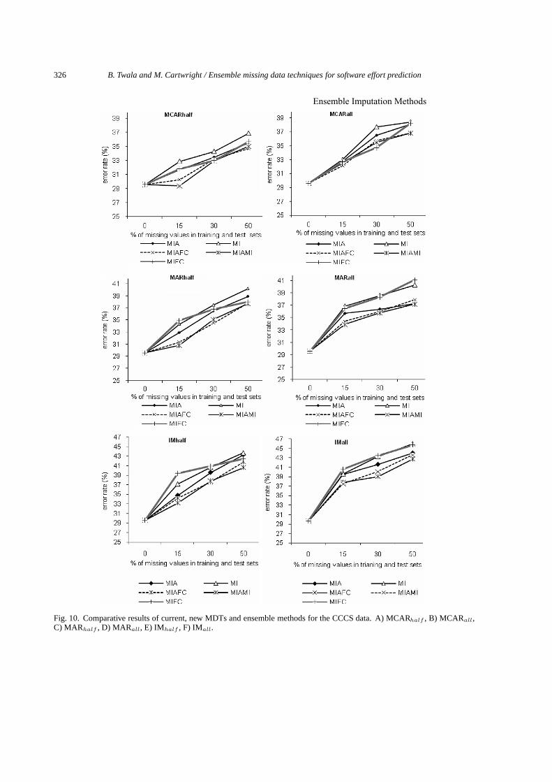
326 B. Twala and M. Cartwright / Ensemble missing data techniques for software effort prediction
Ensemble Imputation Methods
Fig. 10. Comparative results of current, new MDTs and ensemble methods for the CCCS data. A) MCARhalf , B) MCARall,C) MARhalf , D) MARall, E) IMhalf , F) IMall.

B. Twala and M. Cartwright / Ensemble missing data techniques for software effort prediction 327
to perturb the data at each iteration of the imputation algorithm. With fractioning of cases based on MImethods or missing incorporated in attributes, once the weight associated with an observation becomestrivial it may as well be excluded from further iterations of the algorithm because the weight is unlikely torecover to a significant level. With missingness incorporated into attributes based on MI methods this isnot the case. An observation can flip between inclusion and exclusion at each iteration. Another reasonmay be the performance of the individual imputation methods comprising each ensemble methods. MIand MIA consistently dominated the other methods. One strength of MIA that is worth emphasis is theease with which it handles IM data while MI requires the data be MAR. However, even when the MARassumption is violated, MI performs better than several imputation methods. As Schafer [55] points out,the richness of the observed data is related to the plausibility of the MAR assumption. In a multivariatedataset, if the associations among the observed data are reasonably strong, then the observed data mayprovide good information for constructing a model for imputing the missing data.
There are two other advantages of MI, and both involve correcting for the uncertainty of the imputations.One advantage is in the parameter estimates, by essentially taking the mean of the parameter estimatefrom each of the m imputations (where m is the number of imputations). The next advantage of MI isthe correction of standard errors for within and between imputation variance, which allows for betterestimates of confidence intervals and p-values. The strengths of MIA and MI (individually) could be thereason why the combination (ensemble) of the two methods consistently dominates the other methods.
The poor performance of any ensemble with FC as a component could be attributed to the fact that notonly does the strategy fail to exploit or take into account the interrelationships among the attributes, themechanism generating the missing attribute values is unknown. Also, The FC approach works well whenmost of the attributes are independent, because it depends only on their prior distribution of the attributevalues for each attribute being tested in a node of the tree. In other words, the different imputationtreatments differ in how they take advantage of statistical dependencies between attributes.
Our results also show the impact on the performance of methods is caused by the pattern and mechanismof missing values, especially at lower levels of missingness. However, as the proportion of missing valuesincreases, the major determining factor on the performance of methods is how the missing values aredistributed among attributes. All methods yield lower accuracy rates when missing values are distributedamong all the attributes compared with when only one attribute has missing values. The performance ofMI and FC degrade faster as the number of attributes with missing values increases. This was the casefor all the datasets. Also, given that the classification performance of each method varies by mechanismof missing data, it appears that the treatment of missing values not only heavily depends on the missingdata proportions but on the nature of the missing data pattern as well.
The worst performance achieved by methods is for IM data, followed by MCAR and MAR data,respectively. This was a surprising result, which is in not in accordance with statistical theory whichconsiders MCAR as easier to deal with and IM data as very difficult to handle [36].
It was also observed that the impact of missing values depends not just upon a missing data technique,missing data pattern or missing data mechanism but upon a combination of the three. Therefore, neithercan be considered in isolation.
From both experiments, there exists threats to the validity of the results. Potential threats include theinitial exclusion from the datasets of all the instances with missing values, which could have involuntarilyintroduced biases, especially if those missing values contained improtant information and they were notMCAR as we assumed. However, for two of the biggest datasets (Company X and Finnish) theexperimental results were carefully validated. For example, the experiments were conducted under thesupervision of a domain expert who had a deep understanding for each respective underlying dataset.

328 B. Twala and M. Cartwright / Ensemble missing data techniques for software effort prediction
This was a time consumig exercise on ourselves and the experts. The experts were mainly involvedl inthe cleaning up of the datasets in terms of attribute and class noise and outliers. They were also ableto give us reaons why some attributes values were missing. For example, some project managers werereluctant to show projects that had, say, high defect rates. This kind of nonresponse results in IM datawhich otherwise we could not have known.
The averaging of results of the 10 domains/datasets (which is more like mixing datasets from differentcompanies into one dataset) is another potential issue. Some empirical studies in SE assume that domain-and-process factors can be best accounted for within homogenous data, i.e., data produced by the samecompany, with an almost stable process, in the same environment. Hence, in the case of our study, itwould be interesting to see if the results are consistent thorough the ten datasets although results forindividual datastes with certain attribute characterestics was looked at but not into great detail.
The issue of determining whether or not to apply the ensemble strategy to a given dataset must beconsidered. For the work described here, the data were artificially corrupted, i.e. missing values wereartificially simulated on the attributes. Unfortunately, this type of information is rarely known for most“real-world” applications. In some situations, it may be possible to use domain knowledge to determinethe mechanism generating the missing values. For situations where this knowledge is not available,the conservative nature of the consensus ensemble dictates that the data will be missing randomly. Inaddition, fundamentally there are three different classes of missingness mechanism which cover whateversituation one might encounter in practice. Our approach is general since one can apply our results asappropriately. For example, a relevant part of our paper could be taken if an empirical SE researcherthinks he/she has MCAR data. In addition, it is possible to formally test for the MCAR assumption.However, as much as MAR and IM are important, it is hard to test their assumptions, especially for IMdata, which requires one to test for missingness that was deliberately created when data was collected orthe data could be missing due to an unknown censoring mechanism.
This paper has looked at the performance of ensemble imputation methods in terms of smoothedmisclassification error rate. A natural extension would be to consider the impact of such ensemblemethods on other measures of performance, and in particular measures of group separation such as GINIor the magnitude of relative error that is also commonly used to assess classifier performances in theSE industry. MIAMI also deserves further investigation on a number of fronts. First, in terms of thetraining parameters and the combination rules that can be employed. Second, empirical studies of theapplication of MIAMI to datasets from other areas of data mining should be undertaken to assess itsperformance across a more general field. Third, comparisons should be made between MIAMI and otherforms of imputation methods ensembles not investigated in this paper using non-tree-based methods.For example, artificial neural networks and naıve Bayes classifier.
We leave the above issues to be investigated in the future.In sum, this paper provides the beginnings of a better understanding of the relative strengths and
weaknesses of ensemble imputation methods and using decision trees as their component classifier. Itis hoped that it will motivate future theoretical and empirical investigations into incomplete data andsoftware prediction, and perhaps reassure those who are uneasy regarding the use of imputed data insoftware prediction.
Acknowledgements
The authors would like to thank the UK Engineering and Physical Sciences Research Council (undergrant GR/S55347) for funding this research and to the University of Johannesburg, South Africa for

B. Twala and M. Cartwright / Ensemble missing data techniques for software effort prediction 329
additional financial support to finish the research. Further, the authors would like to thank ProfessorDavid Hand and the anonymous revieweres for their invaluable comments on the paper and also forthe contribution from a third sofware organization who provided one of the biggest datasets for thesimulation study but has requested that its identity remains anonymous.
References
[1] E. Bauer and R. Kohavo, An empirical comparison of voting classification algorithms: Bagging, boosting and variants,Machine Learning, 36 1/2 (1989), 105–139.
[2] L. Breiman, Bagging predictors, Machine Learning 26 (2) (1996), 123–140.[3] L. Breiman, Bias, variance, and arcing classifiers, Technical Report 460, Statistics Department, University of California
at Berkeley, 1996b.[4] L. Breiman, J. Friedman, R. Olshen and C. Stone, Classification and Regression Trees, Wadsworth, 1984.[5] L. Briand, V. Basili and W. Thomas, A pattern recognition approach to software engineering data analysis, IEEE
Transactions on Software Engineering 18(11) (1992), 931–942.[6] M. Cartwright and M.J. Shepperd, Building predictive models from object-oriented metrics. 8th European Software
Control and Metrics Conference, Berlin, 1997.[7] M. Cartwright, M.J. Shepperd and Q. Song, Dealing with Missing Software Project Data, In Proceedings of the 9th
International Symposium on Software Metrics, 2003, 154–165.[8] B. Cestnik, I. Kononenko and I. Bratko, Assistant 86: a knowledge-elicitation tool for sophisticated users. In I. Bratko
and N. Lavrac, editors, European Working Session on Learning – EWSL87, Sigma Press, Wilmslow, England, 1987.[9] P. Cheeseman, J. Kelly, M. Self, J. Stutz, W. Taylor and D. Freeman, Bayesian Classification. In Proceedings of American
Association of Artificial Intelligence (AAAI), Morgan Kaufmann Publishers: San Meteo, CA, 1988, 607–611.[10] J. Chen and J. Shao. Nearest Neighbour Imputation for Survey Data. Journal of Official Statistics 16(2) (2000), 113–131.[11] P. Ciaccia, M. Patella and P. Zezula. M-tree: An Efficient Access Method for Similarity Search in Metric Spaces, In
VLDB ’97, 1997, 426–435.[12] A.P. Dempster, N.M. Laird and D.B. Rubin, Maximum likelihood estimation from incomplete data via the EM algorithm,
Journal of the Royal Statistical Society, Series B 39 (1977), 1–38.[13] T.G. Dietterich, An experimental comparison of three methods for constructing ensembles of decision trees: Bagging,
boosting, and randomization, Machine Learning 40(2) (2000), 139–158.[14] T.G. Dietterich, Ensemble Methods in Machine Learning, in: First International Workshop on Multiple Classifier Systems,
Lecture Notes in Computer Science, J. Kittler and F. Roli, eds, 2000, 1–15.[15] J. Dougherty, R. Kohavi and M. Sahami, Supervised and Unsupervised Discretization of Continuous Features, In
Proceedings of the 12th International Conference on Machine Learning, Morgan Kauffmann, Los Altos, CA, 1995.[16] K. El-Emam and A. Birk, Validating the ISO/IEC 15504 Measures of Software Development Process Capability, Journal
of Systems and Software 51(2) (2000), 119–149.[17] M. Evett, T.M. Khoshgoftaar, P. Cheien and E. Allen, GP-based software quality prediction, In Proceedings of the 3rd
Annual Genetic Programming Conference, 1998, 60–65.[18] N. Fenton and M. Neil, A critique of software defect prediction models, IEEE Transactions on Software Engineering
25(5) (1999), 675–689.[19] Y. Freund and R. Schapire, Experiments with a new boosting algorithm, In Machine Learning: Proceedings of the 13th
International Conference, 1996, 148–156.[20] J.W. Graham and S.M. Hofer, EMCOV.EXE user’s Guide (Unpublished Manuscript), University Park, PA: Pennsylvania
State University Department of Bahavioral Health, 1993.[21] T.K. HO, Random decision forests. In Proceedings of the 3rd International Conference on Document Analysis and
Recognition, 1995, 278–282.[22] N. Hollander, W. Sauerbrei and M. Schumacher, Confidence intervals for the effect of a prognostic factor after selection
of an optimal cutpoint, Statistics in Medicine 23 (2004), 1701–1713.[23] ISBSG Data Disk, Release 7, June 2001.[24] I. Jolliffe, Principal Component Analysis, Springer Verlag, 1986.[25] P. Jonsson and C. Wohlin, An Evaluation of k-Nearest Neighbour Imputation Using Likert Data, In Proceedings of the
10th International Symposium on Software Metrics, 108–118, September 11–17, 2004.[26] G.F. Kadoda, M. Cartwright and M. Shepperd, Issues on the Effective Use of CBR Technology for Software Project
Prediction, ICCBR (2001), 276–290.[27] G. Kalton, Compensating for Missing Survey Data, Michigan, 1983.

330 B. Twala and M. Cartwright / Ensemble missing data techniques for software effort prediction
[28] T.M. Khoshgoftaar and N. Seliya, Comparative assessment of software quality classification techniques: an empiricalcase study, Empirical Software Engineering Journal 9(3) (2004), 229–257.
[29] T.M. Khoshgoftaar and N. SELIYA, Tree-based Software Quality Estimation Models for Fault Prediction, In the Pro-ceedings of the 8th IEEE International Symposium on Software Metrics, 2002.
[30] T.M. Khoshgoftaar and E.B. Allen, Modelling Software Quality with Classification Trees, In Recent Advances inReliability and Quality Engineering, Hoang Pham Editor. World Scientific, Singapore, 1999.
[31] T.M. Khoshgoftaar, N. Seliya and A. Herzberg, Resource-oriented software quality classification models, Journal ofSystems and Software 76 (2004), 111–126.
[32] R.E. Kirk, Experimental Design (2nd Ed.), Monterey, CA: Brooks, Cole Publishing Company, 1982.[33] J.O. Kim and J. Curry, The treatment of missing data in multivariate analysis, Sociological Methods and Research 6
(1977), 215–240.[34] K.K. Lai, L. Yu, S.Y. Wang and L.G. Zhou, Credit risk analysis using a reliability-based neural network ensemble model,
Lecture Notes in Computer Science 4132 (2006), 682–690.[35] K. Lakshminarayan, S.A. HARP and T. Samad, Imputation of Missing Data in Industrial Databases, Applied Intelligence
11 (1999), 259–275.[36] R.J.A. Little and D.B. Rubin, Statistical Analysis with Missing Data, New York: Wiley, 1987.[37] M. Mendonca amd N.L. Sunderhaft, Mining Software Engineering Data: A Survey. DACS-SOAR-99-3. A DACS
State-of-theArt Report. DoD Data and Analysis Center for Software, 1999.[38] T. Menzies, Practical Machine Learning for Software Engineering and Knowledge Engineering. In Handbook of Software
Engineering and Knowledge Engineering, 2001. [Available from http://tim.menzies.com/pdf/00ml.pdf, January 2009].[39] MINITAB. MINITAB Statistical Software for Windows 9.0, MINITAB, Inc., PA, USA, 2002.[40] MULTIPLE IMPUTATION SOFTWARE. [Available from http://www.stat.psu.edu/jls/misoftwa.html or http://
methcenter.psu.edu/EMCOV.html; January 2009].[41] O.J. Murphy and R.L. McCraw, Designing storage efficient decision trees, IEEE Transactions on Computing 40(3)
(1991), 315–319.[42] S.K. Murthy and S. Salzberg, Lookahead and pathology in decision tree induction, Proceedings of the 14th International
Joint Conference on Artificial Intelligence, (1992), 309–347, Montreal, Canada: Morgan Kauffman.[43] S. Murthy, S. Kasif and R. Biegel, OC1: Randomised induction of oblique decisions trees, In Proceedings of the 11th
National Conference on Artificial Intelligence, (1993), 322–327.[44] I. Myrtveit, E. Stensrud and U. Olsson, Analyzing Data Sets with Missing Data: An Empirical Evaluation of Imputation
Methods and Likelihood-Based Methods, IEEE Transactions on Software Engineering 27(11) (2001), 1999–1013.[45] D.E. Neumann, An Enhanced Neural Network Technique for Software Risk Analysis, IEEE Transactions on Software
Engineering, (2002), 904–912.[46] E. Papatheocharous and A.S. Andreou, Classification and Prediction of Software Cost through Fuzzy Decision Trees,
Lecture Notes in Business Information Processing 24 (2009), 234–247.[47] A.A. Porter and R.W. Selby, Empirically Guided Software Development Using Metric-Based Classification Trees, IEEE
Software 7(2) (1990), 46–54.[48] A.A. Porter and R.W. Selby, Evaluating Techniques for Generating Metric-based Classification Trees, Journal of Systems
Software (1990), 209–218.[49] J.R. Quinlan, C.4.5: Programs for Machine Learning. Los Altos, California: Morgan Kauffman Publishers, INC., 1993.[50] J.R. Quinlan, Induction to Decision Trees, Machine Learning 1 (1986), 81–106.[51] J.R. Quinlan, Induction over Large Databases: Technical Report HPP-79-14, Stanford University.[52] D.B. Rubin, Multiple Imputation After 18+ Years, Journal of the American Statistical Association 91 (1996), 473–489.[53] S.R. Safavian and D. Landgrebe, A survey of decision tree classifiers, IEEE Transactions on Systems, Man and Cybernetics
21 (1991), 660–674.[54] S.J. Sayyad and T.J. Menzies, The PROMISE Repository of Software Engineering Databases. School of Informa-
tion Technology and Engineering, University of Ottawa, Canada, 2005 [Available from http://promise.site.uottawa.ca/SERepository; January 2009].
[55] J.L. Schafer, Analysis of Incomplete Multivariate Data, Chapman and Hall, London, 1997.[56] J.L. Schafer and M.K. Olsen, Multiple Imputation for multivariate missing data problems: a data analyst’s perspective,
Multivariate Behavioral Research 33(4) (1998), 545–571.[57] J.L. Schafer and J.W. Graham, Missing data: Our view of the state of the art, Psychological Methods 7(2) (2002),
147–177.[58] R.W. Selby and A.A. Porter, Learning from Examples: Generation and Evaluation of Decision Trees for Software
Resource Analysis, IEEE Trans on Soft Eng 14(12) (1988), 1743–1757.[59] P. Sentas, A. Lefteris and I. Stamelos, Multiple Logistic Regression as Imputation method Applied on Software Effort
prediction, In Proceedings of the 10th International Symposium on Software Metrics, Chicago, 14–16 September 2004.[60] A, Shapiro, Structured Induction in Expert Systems, Addison Wesley, London, 1987.

B. Twala and M. Cartwright / Ensemble missing data techniques for software effort prediction 331
[61] M.J. Sheppered and C. Schofiled, Estimating software project using analogies, IEEE Transaction on Software Engineering23(12) (1997), 736–743.
[62] K. Strike, K.E. El-Emam and K.E., Madhavjim, Software Cost Estimation with Incomplete Data, IEEE Transaction onSoftware Engineering 27(10) (2001), 890–908.
[63] Q. Song and M. Sheppered, A Short Note on Safest Default Missingness Mechanism Assumptions, Empirical SoftwareEngineering 10(2) (2005), 235–243.
[64] K. Srinivasan and D. Fisher, Machine Learning Approaches to Estimating Software Development Effort, IEEE Transactionon Software Engineering 21(2) (1995), 126–137.
[65] J. Tian, Integrating Time Domain and Input Domain Analyses of Software Reliability Using Tree-Based Models, IEEETransactions on Software Engineering 21(12) (1995), 945–958.
[66] J. Tian and J. Palma, Analyzing and Improving Reliability: A Tree-based Approach, IEEE Software 15(2) (1998),97–104.
[67] B. Twala, An Empirical Comparison of Techniques Handling Incomplete Data Using Decision Trees, Applied ArtificialIntelligence 23(5) (2009), 373–405.
[68] B. Twala, Effective Techniques for Handling Incomplete Data Using Decision Trees, Unpublished P.hD. Dissetation,Open University, Milton Keynes, UK, 2005.
[69] B. Twala, M.C. Jones and D.J. Hand, Good methods for coping with missing data in decision trees, Pattern RecognitionLetters 29 (2008), 950–956.
[70] B. Twala, M. Cartwright and G. Liebchen, Classifying Incomplete Software Engineering Data Using Decision Trees:An Improved Probabilistic Approach, In Proceedings of Software Engineering Applications, November 13–15, 2006,Dallas, TX, USA.
[71] B. Twala, M.H. Cartwright and M. Shepperd, Comparison of Various Methods for Handling Incomplete Data in SoftwareEngineering Databases, In Proceedings of the 4th International Symposium on Empirical Software Engineering, NoosaHeads, Australia, November 2005.
[72] B. Twala and M.H. Cartwright, Ensemble imputation methods for missing software engineering data, In: Proceedings of11th IEEE International Software Metrics Symposium, 2005, 30–40.
[73] W.N. Venables and B.D. Ripley, Modern Applied Statistics with S-PLUS, New York: Springer, 1994.[74] A.P. White and W.Z. Liu, Bias in information-based measures in decision tree induction, Machine Leaning 15 (1994),
321–329.

Copyright of Intelligent Data Analysis is the property of IOS Press and its content may not be copied or emailed
to multiple sites or posted to a listserv without the copyright holder's express written permission. However,
users may print, download, or email articles for individual use.