enhancing reuse of constraint solutions to improve
TRANSCRIPT

Enhancing Reuse of Constraint Solutions to Improve Symbolic Execution
Xiangyang Jia (Wuhan University)Carlo Ghezzi (Politecnico di Milano)
Shi Ying (Wuhan University)

Outline
❖ Motivation
❖ Logical Basis of our Approach
❖ GreenTrie Framework
❖ Constraint Reduction
❖ Constraint Storing
❖ Constraint Querying
❖ Evaluation
❖ Conclusion and Future Work

Motivation
❖ Symbolic Execution(SE)
❖ A well-known program analysis technique, mainly used for test-case generation and bug finding.
❖ Constraint Solving
❖ The most time-consuming work in SE
❖ Optimization approaches:
❖ Irrelevent constraint elimination
❖ Caching and reuse

Motivation
0
50
100
150
200
250
300
0 0.2 0.4 0.6 0.8 1
Base Irrelevant Constraint Elimination Caching Irrelevant Constraint Elimination + Caching
Aggregated data over 73 applications
Tim
e (s
)
Executed instructions (normalized) 35#
[From Shauvik Roy Choudhary’s Slides]

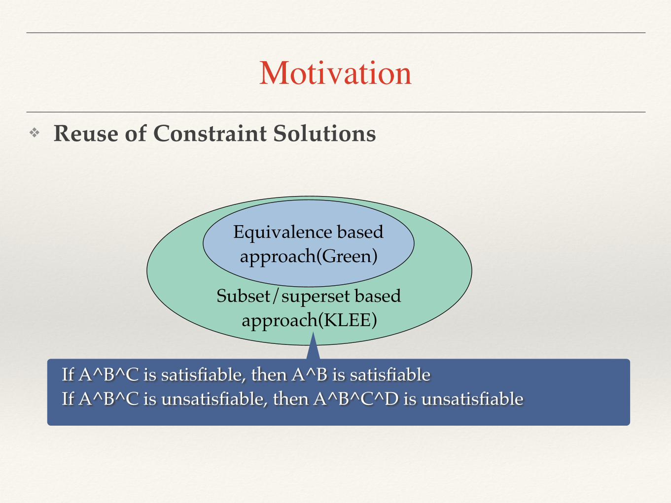
Motivation❖ Reuse of Constraint Solutions
Equivalence based approach(Green)
x>0 is equivalent to y>0x+1>0^ x<=1 is equivalent to y<2 ^y>=0 (if x, y are integers)
Subset/superset based approach(KLEE)
Motivation❖ Reuse of Constraint Solutions
Equivalence based approach(Green)
If A^B^C is satisfiable, then A^B is satisfiableIf A^B^C is unsatisfiable, then A^B^C^D is unsatisfiable

?
Subset/superset based approach(KLEE)
Motivation❖ Reuse of Constraint Solutions
Equivalence based approach(Green)
If x>0 is satisfiable, can we prove x>-1 satisfiable?If x<0^x>1 is unsatisfiable, can we prove x<-1^x>2 unsatisfiable?

Implication based approach(Our approach)
Subset/superset based approach(KLEE)
Motivation❖ Reuse of Constraint Solutions
Equivalence based approach(Green)
If x>0 is satisfiable, can we prove x>-1 satisfiable?If x<0^x>1 is unsatisfiable, can we prove x<-1^x>2 unsatisfiable?

Logical Basis of our Approach
Implication and Satisfiability
It looks easy to apply it to constraint reuse!However, there is a problem: Implication checking with SAT/SMT solver is even more expensive than only solving the single constraint itself.
Providing C1 → C2• if C1 is satisfiable, C2 is satisfiable • if C2 is unsatisfiable, C1 is unsatisfiable
Logical Basis of our Approach
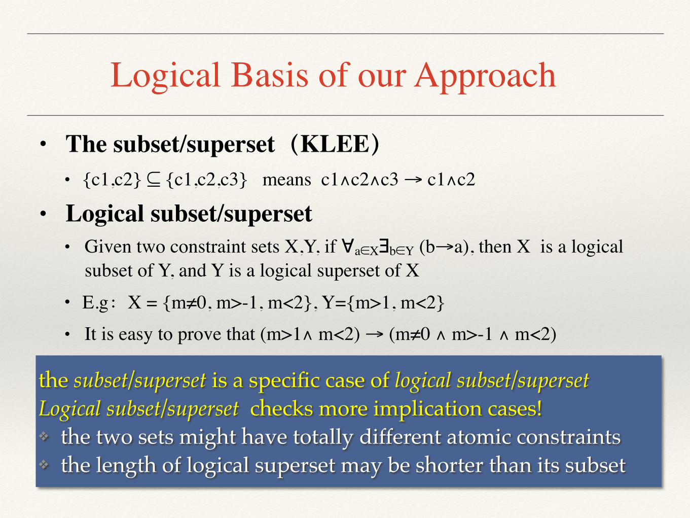
• The subset/superset(KLEE)• {c1,c2} ⊆ {c1,c2,c3} means c1∧c2∧c3 → c1∧c2
• Logical subset/superset • Given two constraint sets X,Y, if ∀a∈X∃b∈Y (b→a), then X is a logical
subset of Y, and Y is a logical superset of X• E.g:X = {m≠0, m>-1, m<2}, Y={m>1, m<2}• It is easy to prove that (m>1∧ m<2) → (m≠0 ∧ m>-1 ∧ m<2)
the subset/superset is a specific case of logical subset/supersetLogical subset/superset checks more implication cases!❖ the two sets might have totally different atomic constraints ❖ the length of logical superset may be shorter than its subset
Logical Basis of our Approach
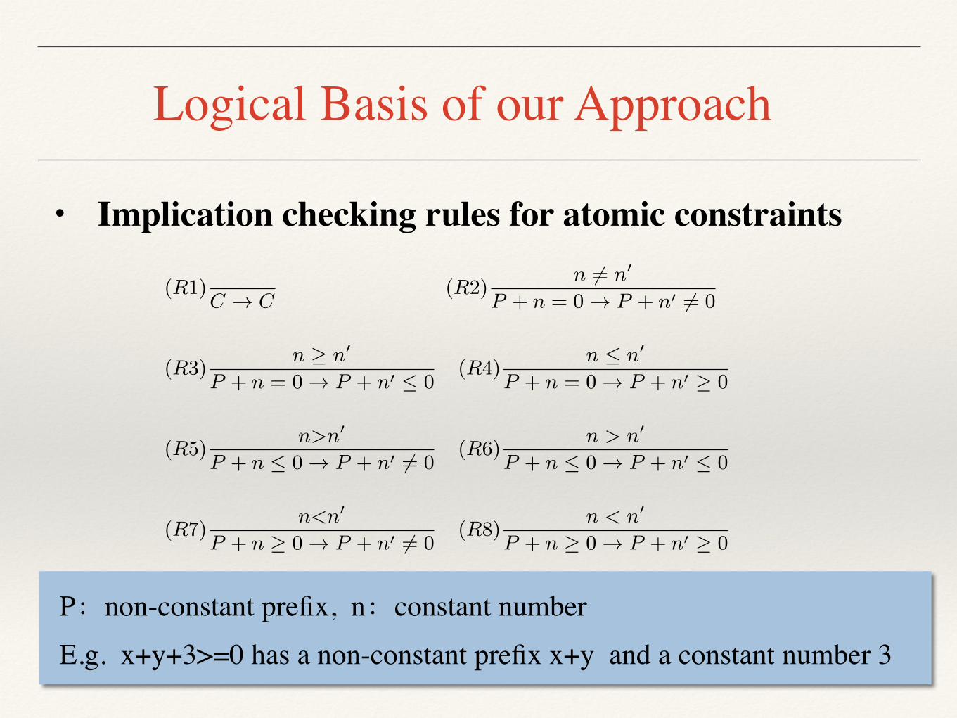
• Implication checking rules for atomic constraints
Proof. (1) Since S is a logical superset of S0, 8c
02S
09c2S
c ! c
0. Hence C1^C2...^Cn
! C
01^C0
2...^C0m
, i.e. C ! C’.According to Lemma 1, if C is satisfiable and has a solutionV, then C
0 is satisfiable and V is also a solutions for C’. (2)Since S is a logical subset of S0, 8
c2S
9c
02S
0c
0 ! c. HenceC
01^C
02...^C
0m
! C1^C2...^C
n
, i.e.C0 ! C. According toLemma 1, if C is unsatisfiable, then C
0 is unsatisfiable.
According to Theorem 1, a constraint can be shown to besatisfiable if a logical superset can be retrieved in a stor-age that caches satisfiable sub-constraint sets. Likewise, aconstraint can be shown to be unsatisfiable if a logical sub-set can be retrieved in a storage that caches unsatisfiablesub-constraint sets.
Normal form of linear integer constraint. In thispaper, every atomic linear integer constraint is canonizedinto the form:
h1v1 + h2v2 + h3v3 + ...h
n
v
n
+ k op 0
where v1, v2...vn are distinct variables, the coe�cients h1,h2..., h
n
are numeric constants, k is an integer constant,h1 � 0, and op 2 {=, 6=,,�}. The expression h1v1+h2v2+h3v3+ ...h
n
v
n
, which contains all non-constant terms, is theconstraint’s non-constant prefix.Implication Checking Rules. We define a list of rules
to check for specific implication relationships between twoatomic linear integer constraints. In this paper, only con-straints which have the same non-constant prefix can bechecked by rules. In the future, we plan to extend therules to handle more complex situations.We compare non-constant prefixes based on string comparison and constantvalues based on numeric comparison, which is quite e�cient.The implication checking rules are listed below. In theserules, P is a non-constant prefix and n is a constant value.The rules enable checking the implication relationship be-tween linear integer arithmetic constraints with operators=, 6=,,�.
(R1)C ! C
(R2)n 6= n
0
P + n = 0 ! P + n
0 6= 0
(R3)n � n
0
P + n = 0 ! P + n
0 0(R4)
n n
0
P + n = 0 ! P + n
0 � 0
(R5)n>n
0
P + n 0 ! P + n
0 6= 0(R6)
n > n
0
P + n 0 ! P + n
0 0
(R7)n<n
0
P + n � 0 ! P + n
0 6= 0(R8)
n < n
0
P + n � 0 ! P + n
0 � 0
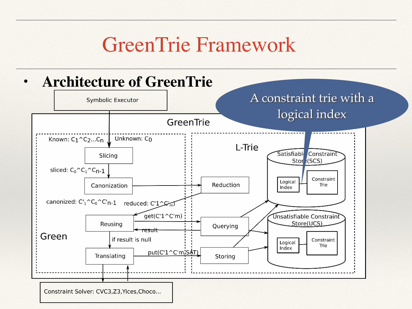
3. OVERVIEW OF GREENTRIEGreenTrie extends the Green framework to improve the
reuse of constraint solutions. The overview architecture ofGreenTrie is illustrated in Fig.1. GreenTrie includes a com-ponent named L-Trie, which replaces the Redis store of theoriginal Green framework. L-Trie is a bipartite store usedfor caching satisfiable and unsatisfiable constraints, respec-tively, each composed of a constraint trie and its logical in-dex. The constraint trie stores constraints in the form ofsub-constraint sets, and the logical index is a partial ordergraph of implication relations for all the sub-constraints inthe trie.
L-Trie and Green work together within GreenTrie. Anyrequest to solve a constraint is handled by Green throughthe following four steps: (1) slicing: it removes pre-solvedirrelevant sub-constraints; (2) canonization: it converts aconstraint into normal form; (3) reusing: it queries the so-lution store for reuse; if a reusable result is not retrieved,(4) translation: the constraint is translated into the in-put format required by the chosen constraint solver (suchas CVC3[18], Z3, Yices[19], or Choco), which is then in-voked to solve the constraint from scratch. The result pro-duced by the constraint solver is finally stored into eithersatisfiable constraint store(SCS) or unsatisfiable constraintstore(UCS)(Fig.1).L-Trie provides three interfaces to Green: constraint re-
duction, constraint querying, and constraint storing. Theseare presented in detail in the following sections. Constraintreduction is performed after the constraint is canonized bythe Green framework; redundant sub-constraints are removedand conflicting sub-constraints are reported in this phase.Constraint querying handles the requests issued by Greento retrieve pre-solved constraints. Based on Theorem 1, itchecks whether the constraint has a logical superset in thesatisfiable constraint store or has a logical subset in the un-satisfiable constraint store. Constraint storing splits solvedconstraint into sub-constraints, puts them into the corre-sponding constraint trie, and the also updates the logicalindex.
4. CONSTRAINT REDUCTIONSymbolic execution conjoins constraints as control flow
branches are traversed. This may introduce redundant sub-constraints, where a sub-constraint is implied by another.For example, if constraint x�0 is conjoined to constraintx 6=-2, the latter becomes redundant and can be eliminated.It may also happen that one can easily detect that the newlyadded constraint conflicts with another constraints, makingthe whole constraint unsatisfiable; for example, consider thecase where x=0 is conjoined with x�3. Constraint reductionin our approach is able to recognize such situations: it canboth reduce the constraint into more concise form and alsofind obviously-conflicted sub-constraints. As we mentioned,we only focus on the linear integer arithmetic constraints.In the future, we plan to reduce other kind of constraintsbased on term rewriting [20].Our approach performs reduction as follows. The sub-
constraints with same non-constant prefix are merged andreduced based on their value interval of non-constant pre-fixes. For example, considering constraint x+y+30, itsnon-constant prefix x+y has a value interval [MIN,�3], andfor constraint x+y�0, the value interval is [0,MAX]. As forconstraint x+y+4=0, the value interval is [4, 4]. If the con-straint is stated as an inequality, as for example x+y+66=0,we have two value intervals [MIN,�6) and (�6,MAX].Equivalently, we can represent this situation by introduc-ing the concept of an exceptional point (in this case, ”-6”).To support reduction, firstly all sub-constraints with the
same non-constant prefix are merged together, by computingthe overlapping interval [A,B] of these constraints, and atthe same time collecting the exceptional points into a setE. For example, after computing of constraint x + y + 3 �0 ^ x+ y + 5 � 0 ^ x+ y � 4 0 ^ x+ y 6= 0 ^ x+ y + 6 6=0^ x+ y� 4 6= 0, we get an overlapping interval [�3, 4] and
P:non-constant prefix, n:constant numberE.g. x+y+3>=0 has a non-constant prefix x+y and a constant number 3

GreenTrie Framework• Architecture of GreenTrie
Figure 1: The overview architecture of GreenTrie
an exceptional point set E = {�6, 0, 4}. After this, we gothrough the following steps:
1. We discard all exceptional points that are outside theoverlapping interval; in the example, the value of E
becomes {0, 4}.
2. If one endpoint of the overlapping interval A (or B)belongs to E, we (repeatedly) change its value andeliminate A (or B) from E at the same time. In theexample after this step the interval becomes [�3, 3]and the new value of E is {0}.
3. If the overlapping interval is empty then the constraintis unsatisfiable and we report a conflict; otherwise wetranslate [A,B] and E into a constraint in normalform. In the example, the final result of our reduc-tion is x+ y + 3 � 0 ^ x+ y � 3 0 ^ x+ y 6= 0.
5. CONSTRAINT STORINGL-Trie provides a di↵erent storage scheme that replaces
the Redis store of Green:
• Unlike Redis, which stores the strings representing con-straints and solutions as key-value pairs, L-Trie splitsconstraints into sub-constraint sets, and stores theminto tries, in order to support logical subset and su-perset queries based on Theorem 1.
• L-Trie stores unsatisfiable and satisfiable constraintsinto separate areas: the Unsatisfiable Constraint Store(UCS) and the Satisfiable Constraint Store (SCS) re-spectively. The two areas are organized di↵erently toe�ciently support logical subset querying and logicalsuperset querying, which pose di↵erent requirements.
• L-Trie maintains a logical index for each of the twotries, to support e�cient check of the implication rela-
tions. The logical index is represented as an implica-tion partial order graph (IPOG), whose nodes containreferences to nodes in the trie.
Both UCS and SCS have the same structure (see Fig. 2).Constraint Trie. The constraint trie is designed to store
a sub-constraint set of solved constraints. The sub-constraintset is sorted in lexicographic order based on string com-parison, to guarantee that sub-constraints with same non-constant prefix are kept close to each other. The labelsof the constraint trie record the sub-constraints. The leafnodes indicate the end of the constraint and are annotatedwith the solution (the solution is null for the leaves of theUCS trie). As shown in Fig.2, the leaf node C2 correspondsto a constraint v0+5>=0 ^v0+v1<=0, which has a solu-tion {v0 : 0,v1 : �1}, and its sub-constraints v0+5>=0 andv0+v1<=0, are annotated as edge labels in the path.If a constraint C is a conjunction of atomic constraints
that is a prefix of another constraint C’ (e.g. C is A^B, andC’ is A ^ B ^ C,), only one of them is kept in the trie. Wekeep the longer constraint in the SCS trie, while we keep theshorter in the UCS trie.Implication Partial Order Graph (IPOG). IPOG is
a graph that contains all the atomic sub-constraints appear-ing in its associated constraint trie, and arranges them asa graph based on the partial order defined by the implica-tion relation. With this graph, given a constraint C, wecan query the sub-constraints which imply C, as well as thesub-constraints which C implies, as we will see later. Thisis useful to improve the e�ciency of implication checkingin logical subset and superset querying. IPOG nodes arelabeled by a sub-constraint and have references to all trienodes whose input edge is labeled with exactly this sub-constraint. Through these references, it is possible to traceall the occurrences of a given sub-constraint.Storing the constraints. Everytime a constraint is
solved (or it is proved to be unsatisfiable), SCS (respec-
Two separated stores for SAT and UNSAT constraints
GreenTrie Framework• Architecture of GreenTrie
Figure 1: The overview architecture of GreenTrie
an exceptional point set E = {�6, 0, 4}. After this, we gothrough the following steps:
1. We discard all exceptional points that are outside theoverlapping interval; in the example, the value of E
becomes {0, 4}.
2. If one endpoint of the overlapping interval A (or B)belongs to E, we (repeatedly) change its value andeliminate A (or B) from E at the same time. In theexample after this step the interval becomes [�3, 3]and the new value of E is {0}.
3. If the overlapping interval is empty then the constraintis unsatisfiable and we report a conflict; otherwise wetranslate [A,B] and E into a constraint in normalform. In the example, the final result of our reduc-tion is x+ y + 3 � 0 ^ x+ y � 3 0 ^ x+ y 6= 0.
5. CONSTRAINT STORINGL-Trie provides a di↵erent storage scheme that replaces
the Redis store of Green:
• Unlike Redis, which stores the strings representing con-straints and solutions as key-value pairs, L-Trie splitsconstraints into sub-constraint sets, and stores theminto tries, in order to support logical subset and su-perset queries based on Theorem 1.
• L-Trie stores unsatisfiable and satisfiable constraintsinto separate areas: the Unsatisfiable Constraint Store(UCS) and the Satisfiable Constraint Store (SCS) re-spectively. The two areas are organized di↵erently toe�ciently support logical subset querying and logicalsuperset querying, which pose di↵erent requirements.
• L-Trie maintains a logical index for each of the twotries, to support e�cient check of the implication rela-
tions. The logical index is represented as an implica-tion partial order graph (IPOG), whose nodes containreferences to nodes in the trie.
Both UCS and SCS have the same structure (see Fig. 2).Constraint Trie. The constraint trie is designed to store
a sub-constraint set of solved constraints. The sub-constraintset is sorted in lexicographic order based on string com-parison, to guarantee that sub-constraints with same non-constant prefix are kept close to each other. The labelsof the constraint trie record the sub-constraints. The leafnodes indicate the end of the constraint and are annotatedwith the solution (the solution is null for the leaves of theUCS trie). As shown in Fig.2, the leaf node C2 correspondsto a constraint v0+5>=0 ^v0+v1<=0, which has a solu-tion {v0 : 0,v1 : �1}, and its sub-constraints v0+5>=0 andv0+v1<=0, are annotated as edge labels in the path.If a constraint C is a conjunction of atomic constraints
that is a prefix of another constraint C’ (e.g. C is A^B, andC’ is A ^ B ^ C,), only one of them is kept in the trie. Wekeep the longer constraint in the SCS trie, while we keep theshorter in the UCS trie.Implication Partial Order Graph (IPOG). IPOG is
a graph that contains all the atomic sub-constraints appear-ing in its associated constraint trie, and arranges them asa graph based on the partial order defined by the implica-tion relation. With this graph, given a constraint C, wecan query the sub-constraints which imply C, as well as thesub-constraints which C implies, as we will see later. Thisis useful to improve the e�ciency of implication checkingin logical subset and superset querying. IPOG nodes arelabeled by a sub-constraint and have references to all trienodes whose input edge is labeled with exactly this sub-constraint. Through these references, it is possible to traceall the occurrences of a given sub-constraint.Storing the constraints. Everytime a constraint is
solved (or it is proved to be unsatisfiable), SCS (respec-
A constraint trie with a logical index

GreenTrie Framework• Architecture of GreenTrie
Figure 1: The overview architecture of GreenTrie
an exceptional point set E = {�6, 0, 4}. After this, we gothrough the following steps:
1. We discard all exceptional points that are outside theoverlapping interval; in the example, the value of E
becomes {0, 4}.
2. If one endpoint of the overlapping interval A (or B)belongs to E, we (repeatedly) change its value andeliminate A (or B) from E at the same time. In theexample after this step the interval becomes [�3, 3]and the new value of E is {0}.
3. If the overlapping interval is empty then the constraintis unsatisfiable and we report a conflict; otherwise wetranslate [A,B] and E into a constraint in normalform. In the example, the final result of our reduc-tion is x+ y + 3 � 0 ^ x+ y � 3 0 ^ x+ y 6= 0.
5. CONSTRAINT STORINGL-Trie provides a di↵erent storage scheme that replaces
the Redis store of Green:
• Unlike Redis, which stores the strings representing con-straints and solutions as key-value pairs, L-Trie splitsconstraints into sub-constraint sets, and stores theminto tries, in order to support logical subset and su-perset queries based on Theorem 1.
• L-Trie stores unsatisfiable and satisfiable constraintsinto separate areas: the Unsatisfiable Constraint Store(UCS) and the Satisfiable Constraint Store (SCS) re-spectively. The two areas are organized di↵erently toe�ciently support logical subset querying and logicalsuperset querying, which pose di↵erent requirements.
• L-Trie maintains a logical index for each of the twotries, to support e�cient check of the implication rela-
tions. The logical index is represented as an implica-tion partial order graph (IPOG), whose nodes containreferences to nodes in the trie.
Both UCS and SCS have the same structure (see Fig. 2).Constraint Trie. The constraint trie is designed to store
a sub-constraint set of solved constraints. The sub-constraintset is sorted in lexicographic order based on string com-parison, to guarantee that sub-constraints with same non-constant prefix are kept close to each other. The labelsof the constraint trie record the sub-constraints. The leafnodes indicate the end of the constraint and are annotatedwith the solution (the solution is null for the leaves of theUCS trie). As shown in Fig.2, the leaf node C2 correspondsto a constraint v0+5>=0 ^v0+v1<=0, which has a solu-tion {v0 : 0,v1 : �1}, and its sub-constraints v0+5>=0 andv0+v1<=0, are annotated as edge labels in the path.If a constraint C is a conjunction of atomic constraints
that is a prefix of another constraint C’ (e.g. C is A^B, andC’ is A ^ B ^ C,), only one of them is kept in the trie. Wekeep the longer constraint in the SCS trie, while we keep theshorter in the UCS trie.Implication Partial Order Graph (IPOG). IPOG is
a graph that contains all the atomic sub-constraints appear-ing in its associated constraint trie, and arranges them asa graph based on the partial order defined by the implica-tion relation. With this graph, given a constraint C, wecan query the sub-constraints which imply C, as well as thesub-constraints which C implies, as we will see later. Thisis useful to improve the e�ciency of implication checkingin logical subset and superset querying. IPOG nodes arelabeled by a sub-constraint and have references to all trienodes whose input edge is labeled with exactly this sub-constraint. Through these references, it is possible to traceall the occurrences of a given sub-constraint.Storing the constraints. Everytime a constraint is
solved (or it is proved to be unsatisfiable), SCS (respec-
remove redundant sub-constraints for better matching

GreenTrie Framework• Architecture of GreenTrie
Figure 1: The overview architecture of GreenTrie
an exceptional point set E = {�6, 0, 4}. After this, we gothrough the following steps:
1. We discard all exceptional points that are outside theoverlapping interval; in the example, the value of E
becomes {0, 4}.
2. If one endpoint of the overlapping interval A (or B)belongs to E, we (repeatedly) change its value andeliminate A (or B) from E at the same time. In theexample after this step the interval becomes [�3, 3]and the new value of E is {0}.
3. If the overlapping interval is empty then the constraintis unsatisfiable and we report a conflict; otherwise wetranslate [A,B] and E into a constraint in normalform. In the example, the final result of our reduc-tion is x+ y + 3 � 0 ^ x+ y � 3 0 ^ x+ y 6= 0.
5. CONSTRAINT STORINGL-Trie provides a di↵erent storage scheme that replaces
the Redis store of Green:
• Unlike Redis, which stores the strings representing con-straints and solutions as key-value pairs, L-Trie splitsconstraints into sub-constraint sets, and stores theminto tries, in order to support logical subset and su-perset queries based on Theorem 1.
• L-Trie stores unsatisfiable and satisfiable constraintsinto separate areas: the Unsatisfiable Constraint Store(UCS) and the Satisfiable Constraint Store (SCS) re-spectively. The two areas are organized di↵erently toe�ciently support logical subset querying and logicalsuperset querying, which pose di↵erent requirements.
• L-Trie maintains a logical index for each of the twotries, to support e�cient check of the implication rela-
tions. The logical index is represented as an implica-tion partial order graph (IPOG), whose nodes containreferences to nodes in the trie.
Both UCS and SCS have the same structure (see Fig. 2).Constraint Trie. The constraint trie is designed to store
a sub-constraint set of solved constraints. The sub-constraintset is sorted in lexicographic order based on string com-parison, to guarantee that sub-constraints with same non-constant prefix are kept close to each other. The labelsof the constraint trie record the sub-constraints. The leafnodes indicate the end of the constraint and are annotatedwith the solution (the solution is null for the leaves of theUCS trie). As shown in Fig.2, the leaf node C2 correspondsto a constraint v0+5>=0 ^v0+v1<=0, which has a solu-tion {v0 : 0,v1 : �1}, and its sub-constraints v0+5>=0 andv0+v1<=0, are annotated as edge labels in the path.If a constraint C is a conjunction of atomic constraints
that is a prefix of another constraint C’ (e.g. C is A^B, andC’ is A ^ B ^ C,), only one of them is kept in the trie. Wekeep the longer constraint in the SCS trie, while we keep theshorter in the UCS trie.Implication Partial Order Graph (IPOG). IPOG is
a graph that contains all the atomic sub-constraints appear-ing in its associated constraint trie, and arranges them asa graph based on the partial order defined by the implica-tion relation. With this graph, given a constraint C, wecan query the sub-constraints which imply C, as well as thesub-constraints which C implies, as we will see later. Thisis useful to improve the e�ciency of implication checkingin logical subset and superset querying. IPOG nodes arelabeled by a sub-constraint and have references to all trienodes whose input edge is labeled with exactly this sub-constraint. Through these references, it is possible to traceall the occurrences of a given sub-constraint.Storing the constraints. Everytime a constraint is
solved (or it is proved to be unsatisfiable), SCS (respec-
❖ Query reusable constraints through logical subset/superset checking

GreenTrie Framework• Architecture of GreenTrie
Figure 1: The overview architecture of GreenTrie
an exceptional point set E = {�6, 0, 4}. After this, we gothrough the following steps:
1. We discard all exceptional points that are outside theoverlapping interval; in the example, the value of E
becomes {0, 4}.
2. If one endpoint of the overlapping interval A (or B)belongs to E, we (repeatedly) change its value andeliminate A (or B) from E at the same time. In theexample after this step the interval becomes [�3, 3]and the new value of E is {0}.
3. If the overlapping interval is empty then the constraintis unsatisfiable and we report a conflict; otherwise wetranslate [A,B] and E into a constraint in normalform. In the example, the final result of our reduc-tion is x+ y + 3 � 0 ^ x+ y � 3 0 ^ x+ y 6= 0.
5. CONSTRAINT STORINGL-Trie provides a di↵erent storage scheme that replaces
the Redis store of Green:
• Unlike Redis, which stores the strings representing con-straints and solutions as key-value pairs, L-Trie splitsconstraints into sub-constraint sets, and stores theminto tries, in order to support logical subset and su-perset queries based on Theorem 1.
• L-Trie stores unsatisfiable and satisfiable constraintsinto separate areas: the Unsatisfiable Constraint Store(UCS) and the Satisfiable Constraint Store (SCS) re-spectively. The two areas are organized di↵erently toe�ciently support logical subset querying and logicalsuperset querying, which pose di↵erent requirements.
• L-Trie maintains a logical index for each of the twotries, to support e�cient check of the implication rela-
tions. The logical index is represented as an implica-tion partial order graph (IPOG), whose nodes containreferences to nodes in the trie.
Both UCS and SCS have the same structure (see Fig. 2).Constraint Trie. The constraint trie is designed to store
a sub-constraint set of solved constraints. The sub-constraintset is sorted in lexicographic order based on string com-parison, to guarantee that sub-constraints with same non-constant prefix are kept close to each other. The labelsof the constraint trie record the sub-constraints. The leafnodes indicate the end of the constraint and are annotatedwith the solution (the solution is null for the leaves of theUCS trie). As shown in Fig.2, the leaf node C2 correspondsto a constraint v0+5>=0 ^v0+v1<=0, which has a solu-tion {v0 : 0,v1 : �1}, and its sub-constraints v0+5>=0 andv0+v1<=0, are annotated as edge labels in the path.If a constraint C is a conjunction of atomic constraints
that is a prefix of another constraint C’ (e.g. C is A^B, andC’ is A ^ B ^ C,), only one of them is kept in the trie. Wekeep the longer constraint in the SCS trie, while we keep theshorter in the UCS trie.Implication Partial Order Graph (IPOG). IPOG is
a graph that contains all the atomic sub-constraints appear-ing in its associated constraint trie, and arranges them asa graph based on the partial order defined by the implica-tion relation. With this graph, given a constraint C, wecan query the sub-constraints which imply C, as well as thesub-constraints which C implies, as we will see later. Thisis useful to improve the e�ciency of implication checkingin logical subset and superset querying. IPOG nodes arelabeled by a sub-constraint and have references to all trienodes whose input edge is labeled with exactly this sub-constraint. Through these references, it is possible to traceall the occurrences of a given sub-constraint.Storing the constraints. Everytime a constraint is
solved (or it is proved to be unsatisfiable), SCS (respec-
❖ If no reusable constraint is found, solve it , and then puts the solving result into stores

Constraint Reduction
Example
x+y+3 ≥ 0 ∧ x+y+5≥0 ∧ x+y−4≤0 ∧ x+y≠0 ∧ x+y+6≠ 0 ∧ x+y−4≠ 0 compute: [-3,∞) ∩ [-5,∞) ∩ (-∞,4] - {0,-6,4} = [-3,4)-{0}reduced: x+y+3 ≥ 0 ∧ x+y-4<0 ∧ x+y≠0
• Constraint Reduction• target: remove redundant sub-constraints• idea: interval computation-based constraint reduction

Constraint Storing
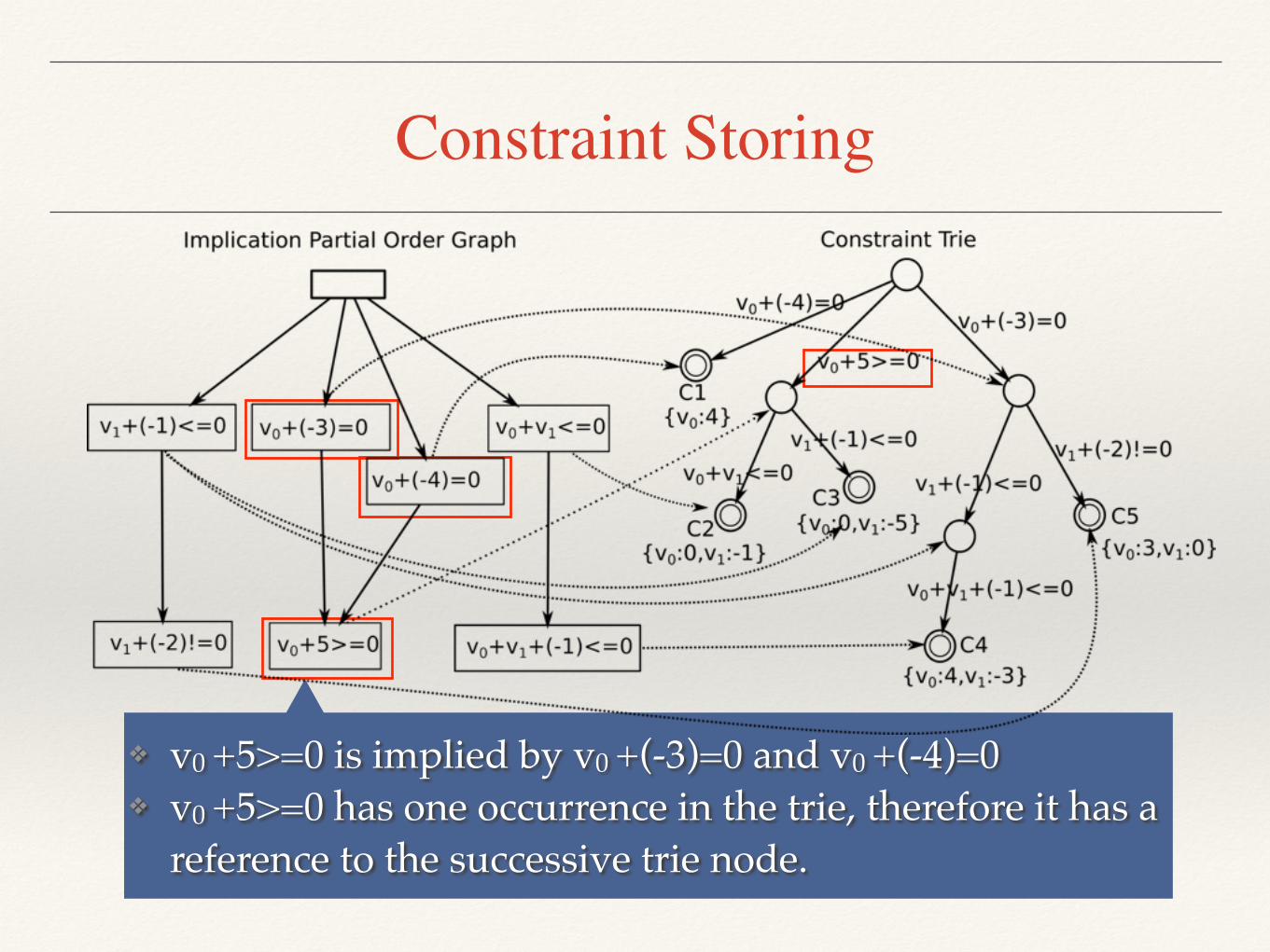
❖ C3 represents a constraint V0+5>=0 ∧ V1+(-1)<=0, which has a solution {v0:0, v1:-5}
Constraint Storing
❖ v0 +5>=0 is implied by v0 +(-3)=0 and v0 +(-4)=0❖ v0 +5>=0 has one occurrence in the trie, therefore it has a
reference to the successive trie node.

Constraint Querying
❖Implication Set(IS) and Reverse Implication Set(RIS)
v0 ≥ 0
ExampleConstraint: v0 ≥ 0ISv0 ≥ 0: {v0 +5>=0}RISv0 ≥ 0: {v0 +(-3)=0, v0 +(-4)=0}

Constraint Querying❖Logical Superset Checking Algorithm
❖Find a path in trie, so that every sub-constraint in target constraint is implied by at least one constraint on this path
ExampleTarget: v0 != 0 ^ v0+(-1)!=0 ^ v1 +(-2)<= 0 RISv1 +(-2)<= 0 : {v1 +(-1)<=0}So, we got two candidate paths to check!
Start from these two nodes!

Constraint Querying
❖Logical Superset Checking Algorithm
ExampleTarget : v0 != 0 ^ v0 +(-1)!= 0 ^ v1+(-2)<= 0RISv0 != 1 : {v0 +(-3)=0,v0 +(-4)=0}
v0+5>=0 is not in the RIS,the trie root is reached,
so this path doesn’t match!

Constraint Querying
❖Logical Superset Checking Algorithm
ExampleTarget: v0 != 0 ^ v0 +(-1)!= 0 ^ v1 +(-2)<= 0RISv0 != 1 : {v0 +(-3)=0,v0 +(-4)=0}
v0+(-3)>=0 is in the RIS, go on to check next sub-constraint
of target!

Constraint Querying
❖Logical Superset Checking Algorithm
ExampleTarget: v0 != 0 ^ v0 +(-1)!= 0 ^ v1 +(-2)<= 0RISv0 != 0 : {v0 +(-3)=0,v0 +(-4)=0}
v0+(-3)>=0 is also in the RIS of v0 != 0, now, every sub-constraint in target is
implied by one constraint on this path.C4 is the reusable constraint!

Constraint Querying❖Logical Subset Checking Algorithm
Target: v0 +(-1)>=0 ^ v0+3!= 0 ^ v0+4<= 0Union of ISs of the sub-constraints : {v0 >=0} ∪ {} ∪ {v0+2<= 0, v0+1<= 0} ISunion ={v0 >=0, v0+2<= 0, v0+1<= 0}We will find a trie path, so that all its sub-constraints on the path exists in ISunion
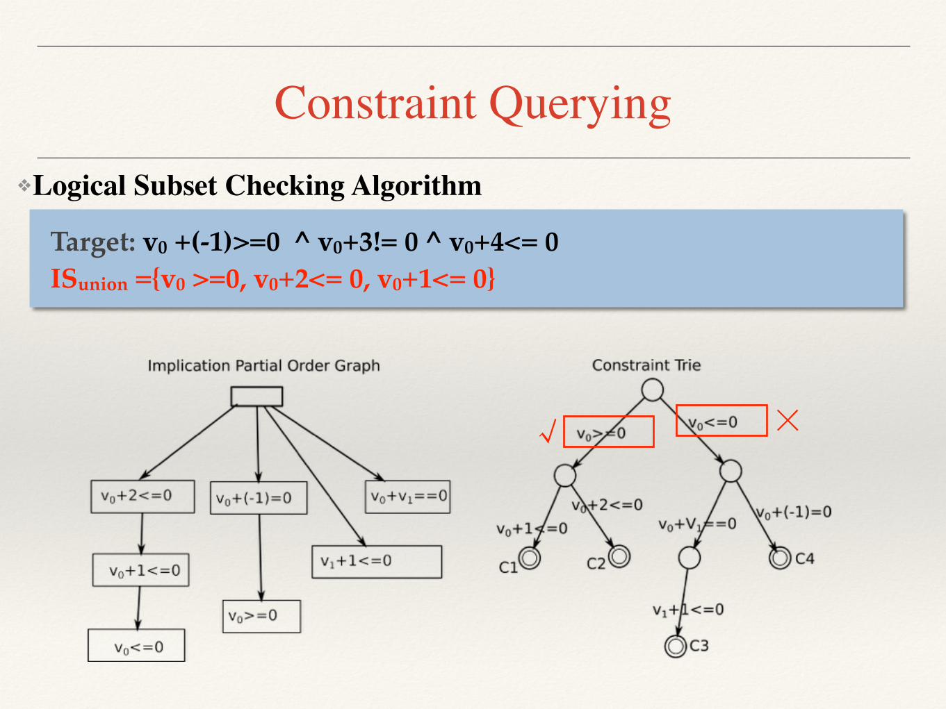
Constraint Querying❖Logical Subset Checking Algorithm
Target: v0 +(-1)>=0 ^ v0+3!= 0 ^ v0+4<= 0ISunion ={v0 >=0, v0+2<= 0, v0+1<= 0}
√ ×

Constraint Querying❖Logical Subset Checking Algorithm
Target: v0 +(-1)>=0 ^ v0+3!= 0 ^ v0+4<= 0ISunion ={v0 >=0, v0+2<= 0, v0+1<= 0}
We found two paths, so the target constraint is unsatisfiable.
√ ×
√√

Evaluation
❖ Research Question
❖ Does GreenTrie achieve better reuse and save more time than other approaches (Green, KLEE) ?
❖ Benchmarks
❖ 6 programs from Green (Willem Visser’s FSE’12 paper)
❖ 1 program from Guowei Yang’s ISSTA 2012 paper.
❖ Experiment scenarios
❖ (1) reuse in a single run of the program
❖ (2) reuse across runs of different versions of the same program
❖ (3) reuse across different programs

Evaluation❖ Experiment setup
❖ PC with a 2.5GHz Intel processor with 4 cores and 4Gb of memory
❖ We implemented GreenTrie by extending Green
❖ We implemented KLEE’s subset/superset checking approach, and also integrated it into Green as an extension.
❖ Symbolic executor: Symbolic Pathfinder (SPF)
❖ Constraint Solver: Z3

Evaluation❖ Reuse in a Single Run
Table 1: Experimental results of reuse in single runProgram n0 n1 n2 n3 R
0R
00t0(ms) t1(ms) t2(ms) t3(ms) T
0T
00
Trityp 32 28 28 28 0.00% 0.00% 1040 915 922 995 -8.74% -7.92%Euclid 642 552 464 464 15.94% 0.00% 5105 6503 7274 6311 2.95% 13.24%TCAS 680 41 20 14 65.85% 30.00% 12742 3356 2182 2165 35.49% 0.78%TreeMap1 24 24 24 24 0.00% 0.00% 871 942 947 882 6.37% 6.86%TreeMap2 148 148 140 140 5.41% 0.00% 2918 2542 2851 2606 -2.52% 8.59%TreeMap3 1080 956 833 806 15.69% 3.24% 21849 10729 11809 9871 8.00% 16.41%BinTree1 84 41 25 25 39.02% 0.00% 1476 1103 1092 1027 6.89% 5.95%BinTree2 472 238 133 118 50.42% 11.28% 4322 3648 3156 2872 21.27% 9.00%BinTree3 3252 1654 939 873 47.22% 7.03% 36581 17197 14764 12041 29.98% 18.44%BinomialHeap1 448 32 23 19 40.63% 17.39% 3637 2137 2046 2017 5.62% 1.42%BinomialHeap2 3184 190 85 68 64.21% 20.00% 27165 7653 6442 6071 20.67% 5.76%BinomialHeap3 23320 988 337 288 70.85% 14.54% 249224 28549 31892 21392 25.07% 32.92%MerArbiter 60648 21 15 13 38.10% 13.33% >10min 304726 290854 272813 10.47% 6.20%total/average 94014 4913 3066 2880 41.38% 6.07% / 390000 374012 341063 12.55% 9.35%
Table 2: Experimental results of reuse across runs (program Euclid)Changes n0 n1 n2 n3 R
0R
00t1(ms) t2(ms) t3(ms) T
0T
00
ADD#1 492 432 5 3 99.54% 60.00% 3896 1375 1329 65.89% 3.35%ADD#2 438 331 216 216 34.74% 0.00% 2830 3275 2284 19.29% 30.26%ADD#3 220 170 32 2 98.82% 93.75% 1382 972 552 60.06% 43.21%DEL#1 438 322 156 126 60.87% 19.23% 3428 2670 2171 36.67% 18.69%DEL#2 492 426 350 134 68.54% 61.71% 3777 4483 2046 45.83% 54.36%DEL#3 642 552 112 111 79.89% 0.89% 4649 2560 2049 55.93% 19.96%MOD#1 642 552 464 463 16.12% 0.22% 4851 6899 4400 9.30% 36.22%MOD#2 642 552 464 462 16.30% 0.43% 4765 7094 4351 8.69% 38.67%MOD#3 642 551 442 433 21.42% 2.04% 4505 7481 4240 5.88% 43.32%
total/average 4648 3888 2241 1949 49.87% 13.03% 34083 36809 23422 31.28% 36.37%
Table 3: Experimental results of reuse across runs (program TCAS)Changes n0 n1 n2 n3 R
0R
00t1(ms) t2(ms) t3(ms) T
0T
00
ADD#1 1036 9 4 2 77.78% 50.00% 1889 1535 1564 17.20% -1.89%ADD#2 2920 4 2 1 75.00% 50.00% 3511 2639 2652 24.47% -0.49%ADD#3 6730 3 0 0 100.00% 0/0 5015 3577 3576 28.69% 0.03%DEL#1 2920 0 0 0 0/0 0/0 2675 2051 2077 22.36% -1.27%DEL#2 1036 0 0 0 0/0 0/0 912 727 807 11.51% -11.00%DEL#3 678 0 0 0 0/0 0/0 632 599 594 6.01% 0.83%MOD#1 1406 2 2 0 100.00% 50.00% 2322 1917 1801 22.44% 6.05%MOD#2 1406 4 2 0 100.00% 50.00% 1888 1490 1440 23.73% 3.36%MOD#3 994 0 0 0 0/0 0/0 1020 817 797 21.86% 2.45%
total/average 19126 22 10 3 86.36% 91.36% 19864 15352 15308 22.94% 0.29%
Table 4: Experimental results of reuse across runs (program BinTree)Changes n0 n1 n2 n3 R
0R
00t1(ms) t2(ms) t3(ms) T
0T
00
ADD#1 5930 1689 803 746 55.83% 7.10% 17978 20355 11889 33.87% 41.59%ADD#2 13358 3938 2618 2556 35.09% 2.37% 35382 105190 32465 8.24% 69.14%ADD#3 15602 540 0 0 100.00% 0/0 18106 61586 17180 5.11% 72.10%DEL#1 13358 3149 2216 2185 30.61% 1.40% 32134 126488 31002 3.52% 75.49%DEL#2 5930 1154 599 0 100.00% 100.00% 13565 44789 10932 19.41% 75.59%DEL#3 3252 1682 0 0 100.00% 0/0 12945 11482 4505 65.20% 60.76%MOD#1 3252 1682 1080 1002 40.43% 7.22% 14553 16297 10628 26.97% 34.79%MOD#2 3252 1680 716 632 62.38% 11.73% 14147 13784 7953 43.78% 42.30%MOD#3 8310 2377 1068 964 59.44% 9.74% 22772 32889 14593 35.92% 55.63%
total/average 72244 17891 9100 8085 54.81% 11.15% 181582 432860 141147 22.27% 67.39%
ni : the number of invocations to solverti : running time for symbolic executioni=0: SE without reuse i=1: SE with Greeni=2: SE with KLEE’s approach i=3: SE with GreenTrieReuse improvement ratio: R’=(n1-n3)/n1 R’’=(n2-n3)/n2
Time improvement ratio: T’=(t1-t3)/t1 T’’=(t2-t3)/t2

Evaluation❖ Reuse in a Single Run
Table 1: Experimental results of reuse in single runProgram n0 n1 n2 n3 R
0R
00t0(ms) t1(ms) t2(ms) t3(ms) T
0T
00
Trityp 32 28 28 28 0.00% 0.00% 1040 915 922 995 -8.74% -7.92%Euclid 642 552 464 464 15.94% 0.00% 5105 6503 7274 6311 2.95% 13.24%TCAS 680 41 20 14 65.85% 30.00% 12742 3356 2182 2165 35.49% 0.78%TreeMap1 24 24 24 24 0.00% 0.00% 871 942 947 882 6.37% 6.86%TreeMap2 148 148 140 140 5.41% 0.00% 2918 2542 2851 2606 -2.52% 8.59%TreeMap3 1080 956 833 806 15.69% 3.24% 21849 10729 11809 9871 8.00% 16.41%BinTree1 84 41 25 25 39.02% 0.00% 1476 1103 1092 1027 6.89% 5.95%BinTree2 472 238 133 118 50.42% 11.28% 4322 3648 3156 2872 21.27% 9.00%BinTree3 3252 1654 939 873 47.22% 7.03% 36581 17197 14764 12041 29.98% 18.44%BinomialHeap1 448 32 23 19 40.63% 17.39% 3637 2137 2046 2017 5.62% 1.42%BinomialHeap2 3184 190 85 68 64.21% 20.00% 27165 7653 6442 6071 20.67% 5.76%BinomialHeap3 23320 988 337 288 70.85% 14.54% 249224 28549 31892 21392 25.07% 32.92%MerArbiter 60648 21 15 13 38.10% 13.33% >10min 304726 290854 272813 10.47% 6.20%total/average 94014 4913 3066 2880 41.38% 6.07% / 390000 374012 341063 12.55% 9.35%
Table 2: Experimental results of reuse across runs (program Euclid)Changes n0 n1 n2 n3 R
0R
00t1(ms) t2(ms) t3(ms) T
0T
00
ADD#1 492 432 5 3 99.54% 60.00% 3896 1375 1329 65.89% 3.35%ADD#2 438 331 216 216 34.74% 0.00% 2830 3275 2284 19.29% 30.26%ADD#3 220 170 32 2 98.82% 93.75% 1382 972 552 60.06% 43.21%DEL#1 438 322 156 126 60.87% 19.23% 3428 2670 2171 36.67% 18.69%DEL#2 492 426 350 134 68.54% 61.71% 3777 4483 2046 45.83% 54.36%DEL#3 642 552 112 111 79.89% 0.89% 4649 2560 2049 55.93% 19.96%MOD#1 642 552 464 463 16.12% 0.22% 4851 6899 4400 9.30% 36.22%MOD#2 642 552 464 462 16.30% 0.43% 4765 7094 4351 8.69% 38.67%MOD#3 642 551 442 433 21.42% 2.04% 4505 7481 4240 5.88% 43.32%
total/average 4648 3888 2241 1949 49.87% 13.03% 34083 36809 23422 31.28% 36.37%
Table 3: Experimental results of reuse across runs (program TCAS)Changes n0 n1 n2 n3 R
0R
00t1(ms) t2(ms) t3(ms) T
0T
00
ADD#1 1036 9 4 2 77.78% 50.00% 1889 1535 1564 17.20% -1.89%ADD#2 2920 4 2 1 75.00% 50.00% 3511 2639 2652 24.47% -0.49%ADD#3 6730 3 0 0 100.00% 0/0 5015 3577 3576 28.69% 0.03%DEL#1 2920 0 0 0 0/0 0/0 2675 2051 2077 22.36% -1.27%DEL#2 1036 0 0 0 0/0 0/0 912 727 807 11.51% -11.00%DEL#3 678 0 0 0 0/0 0/0 632 599 594 6.01% 0.83%MOD#1 1406 2 2 0 100.00% 50.00% 2322 1917 1801 22.44% 6.05%MOD#2 1406 4 2 0 100.00% 50.00% 1888 1490 1440 23.73% 3.36%MOD#3 994 0 0 0 0/0 0/0 1020 817 797 21.86% 2.45%
total/average 19126 22 10 3 86.36% 91.36% 19864 15352 15308 22.94% 0.29%
Table 4: Experimental results of reuse across runs (program BinTree)Changes n0 n1 n2 n3 R
0R
00t1(ms) t2(ms) t3(ms) T
0T
00
ADD#1 5930 1689 803 746 55.83% 7.10% 17978 20355 11889 33.87% 41.59%ADD#2 13358 3938 2618 2556 35.09% 2.37% 35382 105190 32465 8.24% 69.14%ADD#3 15602 540 0 0 100.00% 0/0 18106 61586 17180 5.11% 72.10%DEL#1 13358 3149 2216 2185 30.61% 1.40% 32134 126488 31002 3.52% 75.49%DEL#2 5930 1154 599 0 100.00% 100.00% 13565 44789 10932 19.41% 75.59%DEL#3 3252 1682 0 0 100.00% 0/0 12945 11482 4505 65.20% 60.76%MOD#1 3252 1682 1080 1002 40.43% 7.22% 14553 16297 10628 26.97% 34.79%MOD#2 3252 1680 716 632 62.38% 11.73% 14147 13784 7953 43.78% 42.30%MOD#3 8310 2377 1068 964 59.44% 9.74% 22772 32889 14593 35.92% 55.63%
total/average 72244 17891 9100 8085 54.81% 11.15% 181582 432860 141147 22.27% 67.39%
GreenTrie gets better reuse ratio and saves more time when the scale of execution increases.

Table 1: Experimental results of reuse in single runProgram n0 n1 n2 n3 R
0R
00t0(ms) t1(ms) t2(ms) t3(ms) T
0T
00
Trityp 32 28 28 28 0.00% 0.00% 1040 915 922 995 -8.74% -7.92%Euclid 642 552 464 464 15.94% 0.00% 5105 6503 7274 6311 2.95% 13.24%TCAS 680 41 20 14 65.85% 30.00% 12742 3356 2182 2165 35.49% 0.78%TreeMap1 24 24 24 24 0.00% 0.00% 871 942 947 882 6.37% 6.86%TreeMap2 148 148 140 140 5.41% 0.00% 2918 2542 2851 2606 -2.52% 8.59%TreeMap3 1080 956 833 806 15.69% 3.24% 21849 10729 11809 9871 8.00% 16.41%BinTree1 84 41 25 25 39.02% 0.00% 1476 1103 1092 1027 6.89% 5.95%BinTree2 472 238 133 118 50.42% 11.28% 4322 3648 3156 2872 21.27% 9.00%BinTree3 3252 1654 939 873 47.22% 7.03% 36581 17197 14764 12041 29.98% 18.44%BinomialHeap1 448 32 23 19 40.63% 17.39% 3637 2137 2046 2017 5.62% 1.42%BinomialHeap2 3184 190 85 68 64.21% 20.00% 27165 7653 6442 6071 20.67% 5.76%BinomialHeap3 23320 988 337 288 70.85% 14.54% 249224 28549 31892 21392 25.07% 32.92%MerArbiter 60648 21 15 13 38.10% 13.33% >10min 304726 290854 272813 10.47% 6.20%total/average 94014 4913 3066 2880 41.38% 6.07% / 390000 374012 341063 12.55% 9.35%
Table 2: Experimental results of reuse across runs (program Euclid)Changes n0 n1 n2 n3 R
0R
00t1(ms) t2(ms) t3(ms) T
0T
00
ADD#1 492 432 5 3 99.54% 60.00% 3896 1375 1329 65.89% 3.35%ADD#2 438 331 216 216 34.74% 0.00% 2830 3275 2284 19.29% 30.26%ADD#3 220 170 32 2 98.82% 93.75% 1382 972 552 60.06% 43.21%DEL#1 438 322 156 126 60.87% 19.23% 3428 2670 2171 36.67% 18.69%DEL#2 492 426 350 134 68.54% 61.71% 3777 4483 2046 45.83% 54.36%DEL#3 642 552 112 111 79.89% 0.89% 4649 2560 2049 55.93% 19.96%MOD#1 642 552 464 463 16.12% 0.22% 4851 6899 4400 9.30% 36.22%MOD#2 642 552 464 462 16.30% 0.43% 4765 7094 4351 8.69% 38.67%MOD#3 642 551 442 433 21.42% 2.04% 4505 7481 4240 5.88% 43.32%
total/average 4648 3888 2241 1949 49.87% 13.03% 34083 36809 23422 31.28% 36.37%
Table 3: Experimental results of reuse across runs (program TCAS)Changes n0 n1 n2 n3 R
0R
00t1(ms) t2(ms) t3(ms) T
0T
00
ADD#1 1036 9 4 2 77.78% 50.00% 1889 1535 1564 17.20% -1.89%ADD#2 2920 4 2 1 75.00% 50.00% 3511 2639 2652 24.47% -0.49%ADD#3 6730 3 0 0 100.00% 0/0 5015 3577 3576 28.69% 0.03%DEL#1 2920 0 0 0 0/0 0/0 2675 2051 2077 22.36% -1.27%DEL#2 1036 0 0 0 0/0 0/0 912 727 807 11.51% -11.00%DEL#3 678 0 0 0 0/0 0/0 632 599 594 6.01% 0.83%MOD#1 1406 2 2 0 100.00% 50.00% 2322 1917 1801 22.44% 6.05%MOD#2 1406 4 2 0 100.00% 50.00% 1888 1490 1440 23.73% 3.36%MOD#3 994 0 0 0 0/0 0/0 1020 817 797 21.86% 2.45%
total/average 19126 22 10 3 86.36% 91.36% 19864 15352 15308 22.94% 0.29%
Table 4: Experimental results of reuse across runs (program BinTree)Changes n0 n1 n2 n3 R
0R
00t1(ms) t2(ms) t3(ms) T
0T
00
ADD#1 5930 1689 803 746 55.83% 7.10% 17978 20355 11889 33.87% 41.59%ADD#2 13358 3938 2618 2556 35.09% 2.37% 35382 105190 32465 8.24% 69.14%ADD#3 15602 540 0 0 100.00% 0/0 18106 61586 17180 5.11% 72.10%DEL#1 13358 3149 2216 2185 30.61% 1.40% 32134 126488 31002 3.52% 75.49%DEL#2 5930 1154 599 0 100.00% 100.00% 13565 44789 10932 19.41% 75.59%DEL#3 3252 1682 0 0 100.00% 0/0 12945 11482 4505 65.20% 60.76%MOD#1 3252 1682 1080 1002 40.43% 7.22% 14553 16297 10628 26.97% 34.79%MOD#2 3252 1680 716 632 62.38% 11.73% 14147 13784 7953 43.78% 42.30%MOD#3 8310 2377 1068 964 59.44% 9.74% 22772 32889 14593 35.92% 55.63%
total/average 72244 17891 9100 8085 54.81% 11.15% 181582 432860 141147 22.27% 67.39%
Evaluation❖ Reuse across Runs
GreenTrie gets better reuse ratio and saves more time than both Green and KLEE’s approach.
Table 1: Experimental results of reuse in single runProgram n0 n1 n2 n3 R
0R
00t0(ms) t1(ms) t2(ms) t3(ms) T
0T
00
Trityp 32 28 28 28 0.00% 0.00% 1040 915 922 995 -8.74% -7.92%Euclid 642 552 464 464 15.94% 0.00% 5105 6503 7274 6311 2.95% 13.24%TCAS 680 41 20 14 65.85% 30.00% 12742 3356 2182 2165 35.49% 0.78%TreeMap1 24 24 24 24 0.00% 0.00% 871 942 947 882 6.37% 6.86%TreeMap2 148 148 140 140 5.41% 0.00% 2918 2542 2851 2606 -2.52% 8.59%TreeMap3 1080 956 833 806 15.69% 3.24% 21849 10729 11809 9871 8.00% 16.41%BinTree1 84 41 25 25 39.02% 0.00% 1476 1103 1092 1027 6.89% 5.95%BinTree2 472 238 133 118 50.42% 11.28% 4322 3648 3156 2872 21.27% 9.00%BinTree3 3252 1654 939 873 47.22% 7.03% 36581 17197 14764 12041 29.98% 18.44%BinomialHeap1 448 32 23 19 40.63% 17.39% 3637 2137 2046 2017 5.62% 1.42%BinomialHeap2 3184 190 85 68 64.21% 20.00% 27165 7653 6442 6071 20.67% 5.76%BinomialHeap3 23320 988 337 288 70.85% 14.54% 249224 28549 31892 21392 25.07% 32.92%MerArbiter 60648 21 15 13 38.10% 13.33% >10min 304726 290854 272813 10.47% 6.20%total/average 94014 4913 3066 2880 41.38% 6.07% / 390000 374012 341063 12.55% 9.35%
Table 2: Experimental results of reuse across runs (program Euclid)Changes n0 n1 n2 n3 R
0R
00t1(ms) t2(ms) t3(ms) T
0T
00
ADD#1 492 432 5 3 99.54% 60.00% 3896 1375 1329 65.89% 3.35%ADD#2 438 331 216 216 34.74% 0.00% 2830 3275 2284 19.29% 30.26%ADD#3 220 170 32 2 98.82% 93.75% 1382 972 552 60.06% 43.21%DEL#1 438 322 156 126 60.87% 19.23% 3428 2670 2171 36.67% 18.69%DEL#2 492 426 350 134 68.54% 61.71% 3777 4483 2046 45.83% 54.36%DEL#3 642 552 112 111 79.89% 0.89% 4649 2560 2049 55.93% 19.96%MOD#1 642 552 464 463 16.12% 0.22% 4851 6899 4400 9.30% 36.22%MOD#2 642 552 464 462 16.30% 0.43% 4765 7094 4351 8.69% 38.67%MOD#3 642 551 442 433 21.42% 2.04% 4505 7481 4240 5.88% 43.32%
total/average 4648 3888 2241 1949 49.87% 13.03% 34083 36809 23422 31.28% 36.37%
Table 3: Experimental results of reuse across runs (program TCAS)Changes n0 n1 n2 n3 R
0R
00t1(ms) t2(ms) t3(ms) T
0T
00
ADD#1 1036 9 4 2 77.78% 50.00% 1889 1535 1564 17.20% -1.89%ADD#2 2920 4 2 1 75.00% 50.00% 3511 2639 2652 24.47% -0.49%ADD#3 6730 3 0 0 100.00% 0/0 5015 3577 3576 28.69% 0.03%DEL#1 2920 0 0 0 0/0 0/0 2675 2051 2077 22.36% -1.27%DEL#2 1036 0 0 0 0/0 0/0 912 727 807 11.51% -11.00%DEL#3 678 0 0 0 0/0 0/0 632 599 594 6.01% 0.83%MOD#1 1406 2 2 0 100.00% 50.00% 2322 1917 1801 22.44% 6.05%MOD#2 1406 4 2 0 100.00% 50.00% 1888 1490 1440 23.73% 3.36%MOD#3 994 0 0 0 0/0 0/0 1020 817 797 21.86% 2.45%
total/average 19126 22 10 3 86.36% 91.36% 19864 15352 15308 22.94% 0.29%
Table 4: Experimental results of reuse across runs (program BinTree)Changes n0 n1 n2 n3 R
0R
00t1(ms) t2(ms) t3(ms) T
0T
00
ADD#1 5930 1689 803 746 55.83% 7.10% 17978 20355 11889 33.87% 41.59%ADD#2 13358 3938 2618 2556 35.09% 2.37% 35382 105190 32465 8.24% 69.14%ADD#3 15602 540 0 0 100.00% 0/0 18106 61586 17180 5.11% 72.10%DEL#1 13358 3149 2216 2185 30.61% 1.40% 32134 126488 31002 3.52% 75.49%DEL#2 5930 1154 599 0 100.00% 100.00% 13565 44789 10932 19.41% 75.59%DEL#3 3252 1682 0 0 100.00% 0/0 12945 11482 4505 65.20% 60.76%MOD#1 3252 1682 1080 1002 40.43% 7.22% 14553 16297 10628 26.97% 34.79%MOD#2 3252 1680 716 632 62.38% 11.73% 14147 13784 7953 43.78% 42.30%MOD#3 8310 2377 1068 964 59.44% 9.74% 22772 32889 14593 35.92% 55.63%
total/average 72244 17891 9100 8085 54.81% 11.15% 181582 432860 141147 22.27% 67.39%

Evaluation
❖ Reuse across Runs
Table 1: Experimental results of reuse in single runProgram n0 n1 n2 n3 R
0R
00t0(ms) t1(ms) t2(ms) t3(ms) T
0T
00
Trityp 32 28 28 28 0.00% 0.00% 1040 915 922 995 -8.74% -7.92%Euclid 642 552 464 464 15.94% 0.00% 5105 6503 7274 6311 2.95% 13.24%TCAS 680 41 20 14 65.85% 30.00% 12742 3356 2182 2165 35.49% 0.78%TreeMap1 24 24 24 24 0.00% 0.00% 871 942 947 882 6.37% 6.86%TreeMap2 148 148 140 140 5.41% 0.00% 2918 2542 2851 2606 -2.52% 8.59%TreeMap3 1080 956 833 806 15.69% 3.24% 21849 10729 11809 9871 8.00% 16.41%BinTree1 84 41 25 25 39.02% 0.00% 1476 1103 1092 1027 6.89% 5.95%BinTree2 472 238 133 118 50.42% 11.28% 4322 3648 3156 2872 21.27% 9.00%BinTree3 3252 1654 939 873 47.22% 7.03% 36581 17197 14764 12041 29.98% 18.44%BinomialHeap1 448 32 23 19 40.63% 17.39% 3637 2137 2046 2017 5.62% 1.42%BinomialHeap2 3184 190 85 68 64.21% 20.00% 27165 7653 6442 6071 20.67% 5.76%BinomialHeap3 23320 988 337 288 70.85% 14.54% 249224 28549 31892 21392 25.07% 32.92%MerArbiter 60648 21 15 13 38.10% 13.33% >10min 304726 290854 272813 10.47% 6.20%total/average 94014 4913 3066 2880 41.38% 6.07% / 390000 374012 341063 12.55% 9.35%
Table 2: Experimental results of reuse across runs (program Euclid)Changes n0 n1 n2 n3 R
0R
00t1(ms) t2(ms) t3(ms) T
0T
00
ADD#1 492 432 5 3 99.54% 60.00% 3896 1375 1329 65.89% 3.35%ADD#2 438 331 216 216 34.74% 0.00% 2830 3275 2284 19.29% 30.26%ADD#3 220 170 32 2 98.82% 93.75% 1382 972 552 60.06% 43.21%DEL#1 438 322 156 126 60.87% 19.23% 3428 2670 2171 36.67% 18.69%DEL#2 492 426 350 134 68.54% 61.71% 3777 4483 2046 45.83% 54.36%DEL#3 642 552 112 111 79.89% 0.89% 4649 2560 2049 55.93% 19.96%MOD#1 642 552 464 463 16.12% 0.22% 4851 6899 4400 9.30% 36.22%MOD#2 642 552 464 462 16.30% 0.43% 4765 7094 4351 8.69% 38.67%MOD#3 642 551 442 433 21.42% 2.04% 4505 7481 4240 5.88% 43.32%
total/average 4648 3888 2241 1949 49.87% 13.03% 34083 36809 23422 31.28% 36.37%
Table 3: Experimental results of reuse across runs (program TCAS)Changes n0 n1 n2 n3 R
0R
00t1(ms) t2(ms) t3(ms) T
0T
00
ADD#1 1036 9 4 2 77.78% 50.00% 1889 1535 1564 17.20% -1.89%ADD#2 2920 4 2 1 75.00% 50.00% 3511 2639 2652 24.47% -0.49%ADD#3 6730 3 0 0 100.00% 0/0 5015 3577 3576 28.69% 0.03%DEL#1 2920 0 0 0 0/0 0/0 2675 2051 2077 22.36% -1.27%DEL#2 1036 0 0 0 0/0 0/0 912 727 807 11.51% -11.00%DEL#3 678 0 0 0 0/0 0/0 632 599 594 6.01% 0.83%MOD#1 1406 2 2 0 100.00% 50.00% 2322 1917 1801 22.44% 6.05%MOD#2 1406 4 2 0 100.00% 50.00% 1888 1490 1440 23.73% 3.36%MOD#3 994 0 0 0 0/0 0/0 1020 817 797 21.86% 2.45%
total/average 19126 22 10 3 86.36% 91.36% 19864 15352 15308 22.94% 0.29%
Table 4: Experimental results of reuse across runs (program BinTree)Changes n0 n1 n2 n3 R
0R
00t1(ms) t2(ms) t3(ms) T
0T
00
ADD#1 5930 1689 803 746 55.83% 7.10% 17978 20355 11889 33.87% 41.59%ADD#2 13358 3938 2618 2556 35.09% 2.37% 35382 105190 32465 8.24% 69.14%ADD#3 15602 540 0 0 100.00% 0/0 18106 61586 17180 5.11% 72.10%DEL#1 13358 3149 2216 2185 30.61% 1.40% 32134 126488 31002 3.52% 75.49%DEL#2 5930 1154 599 0 100.00% 100.00% 13565 44789 10932 19.41% 75.59%DEL#3 3252 1682 0 0 100.00% 0/0 12945 11482 4505 65.20% 60.76%MOD#1 3252 1682 1080 1002 40.43% 7.22% 14553 16297 10628 26.97% 34.79%MOD#2 3252 1680 716 632 62.38% 11.73% 14147 13784 7953 43.78% 42.30%MOD#3 8310 2377 1068 964 59.44% 9.74% 22772 32889 14593 35.92% 55.63%
total/average 72244 17891 9100 8085 54.81% 11.15% 181582 432860 141147 22.27% 67.39%
GreenTrie gains better scalability than KLEE’s approach
3421 constraints in store
Running time increases dramatically in KLEE’s
approach

Evaluation❖ Reuse across Programs
Table 5: Experimental results of reuse across programsProgram Trityp Euclid TCAS TreeMap BinTree BinomialHeap MerArbiterTrityp / 0, 0, 3 0, 0, 3 0, 4, 4 0, 2, 2 0, 6, 7 0, 0, 1Euclid 0, 0, 1 / 2, 5, 5 0, 0, 0 0, 3, 4 0, 2, 2 0, 0, 2TCAS 0, 0, 2 2, 2, 2 / 0, 0, 0 0, 2, 3 0, 3, 4 0, 3, 4TreeMap 0, 0, 0 0, 0, 0 0, 0, 0 / 256, 326, 323 0, 0, 0 0, 0, 0BinTree 0, 0, 0 0, 0, 0 0, 0, 0 256, 449, 470 / 0, 1, 1 0, 0, 0BinomialHeap 2, 2, 5 2, 2, 5 2, 8, 6 0, 2, 3 1, 11, 10 / 0, 0, 0MerArbiter 0, 1, 2 0, 2 0, 3 0, 0, 0 0, 0, 0 0, 0, 0 /
We also have shown that GreenTrie saves symbolic execu-tion time with respect to Green and KLEE. One reason isthat, because of its higher reuse ratio, it invokes the solverless times than Green. Another reason is that the logicalsuperset and subset querying algorithm is performed as ef-ficiently or even better than that in Green and KLEE. Asshown in the experiments of Section 7.2, when both Green-Trie, Green, and KLEE all gain high reuse ratios, GreenTrieis still faster than other two approaches.
Unlike Green, which uses Redis to store and query solu-tions, GreenTrie saves SCS and UCS as two files on disk andloads them into memory when symbolic execution is started.GreenTrie uses almost the same memory as Green for sym-bolic execution. For example, in the case of Bintree-3 inSection 7.1, GreenTrie uses 284Mb memory, and Green uses288Mb (including 5M due to the Redis process). Green-Trie also optimizes the space occupied by L-Tries: each ex-pression is an object (a sub-constraint is also an expressioncomposed by smaller expressions), and its occurrences in dif-ferent constraints in the trie and the IPOG are all referencesto this object. Since the constraints in symbolic executionare always composed by the same group of expressions/sub-constraints, this optimization significantly decreases the spaceoccupied by L-Tries. As an example, in the case of Bintree-3 the total size of SCS and UCS stores is 387 Kb for 873cached constraints composed with 81 expressions.
GreenTrie has one limitation compared to the originalGreen framework: by now GreenTrie is only able to reuse theSAT solving results, and cannot reuse the model countingresults (that are utilized to calculate path execution proba-bilities[24]) as Green instead does.
9. CONCLUSION AND FUTURE WORKWe introduced a new approach to reuse the constraint
solving results in symbolic execution based on their logi-cal relations. We presented GreenTrie, an extension to theGreen framework, which stores constraints and solutionsinto two tries indexed by implication partial order graphs.GreenTrie is able to carry out logical reduction and log-ical subset and superset querying for given constraint, tocheck if any solutions in stores can be reused. As our exper-imental results show, GreenTrie not only saves considerablesymbolic execution time with respect to the case where con-straint evaluations are not reused, but also achieves betterreuse and saves significant time with respect to Green andKLEE approach.
Our future work will extend GreenTrie to support morekinds of constraints other than linear integer constraints,through adding implication rules and extending query al-gorithm, as well as introducing the term rewriting tech-nique[20] to simplify the complex constraints. We also plan
to make the summaries in compositional symbolic execu-tion[25, 26] reusable at a finer granularity, considering thatthe summary is a disjunctive constraint that composed bypre and post conditions of paths of target method. Thiswork is part of our long-term e↵orts that aim at supportingincremental and agile verification[27, 28, 29].
10. ACKNOWLEDGMENTSWe thank Domenico Bianculli, Srdjan Krstic, Giovanni
Denaro, Mauro Pezze, Pietro Braione for comments andsuggestions in various stages of this work. This work wassupported by European Commission, Program IDEAS-ERC,Project 227977-SMScom, National Natural Science Founda-tion of China under Grant No.61272108, No.91118003 andNo.61373038, and the National High Technology Researchand Development Program of China, No. 2012AA011204-01.
11. REFERENCES[1] James C. King. Symbolic execution and program
testing. Communications of the ACM, 19(7):385–394,July 1976.
[2] Ella Bounimova, Patrice Godefroid, and DavidMolnar. Billions and billions of constraints: whiteboxfuzz testing in production. In Proceedings of the 2013International Conference on Software Engineering,pages 122–131. IEEE Press, May 2013.
[3] Thanassis Avgerinos, Alexandre Rebert, Sang KilCha, and David Brumley. Enhancing SymbolicExecution with Veritesting. In Proceedings of the 36thInternational Conference on Software Engineering -ICSE 2014, pages 1083–1094, Hyderabad, May 2014.ACM Press.
[4] Cristian Cadar and Koushik Sen. Symbolic executionfor software testing: three decades later.Communications of the ACM, 56(2):82–90, 2013.
[5] Corina S. Pasareanu and Willem Visser. A survey ofnew trends in symbolic execution for software testingand analysis. International Journal on Software Toolsfor Technology Transfer, 11(4):339–353, August 2009.
[6] Saswat Anand. Techniques to facilitate symbolicexecution of real-world programs. PhD thesis, GeorgiaInstitute of Technology, 2012.
[7] Koushik Sen, Darko Marinov, and Gul Agha. CUTE:A concolic unit testing engine for C. In Proceedings ofthe 10th European software engineering conferenceheld jointly with 13th ACM SIGSOFT internationalsymposium on Foundations of software engineering -ESEC/FSE-13, pages 263–272, New York, USA,September 2005. ACM Press.
Numbers of reused constraints for Green, KLEE approach and GreenTrie
GreenTrie achieves more inter-programs reuse than Green.In some cases, GreenTrie has a little less reuse than KLEE’s approach. The reason is that some constraints, which reuse the solution both across programs and in same program in GreenTrie, can only reuse constraints across programs in KLEE. Such constraints are counted for KLEE but not counted for GreenTrie

Conclusion and Future Work
❖ Contributions
❖ Logical basis of implication-based reuse
❖ Trie-based store indexed with implication partial order graph
❖ Efficient logical subset/superset checking algorithms
❖ Future works
❖ Support more kinds of constraints other than linear integer constraints
❖ Reuse constraints which contains summaries
❖ Improve scalability for large-scale programs

Apologize
❖ I am sorry that I cannot answer your question face to face.
❖ If you have any question, please contact me with this email: