enhancement of emag: a 2-d electrostatic and … · magnetostatic solver for matlab wells, david...
TRANSCRIPT

Calhoun: The NPS Institutional Archive
Theses and Dissertations Thesis Collection
1994-09
Enhancement of EMAG: a 2-D electrostatic and
magnetostatic solver for MATLAB
Wells, David Patrick
Monterey, California. Naval Postgraduate School
http://hdl.handle.net/10945/43041

, ..
NAVAL POSTGRADUATE SCHOOL Monterey, California
AD-A283 446 11111111111..---
DTIC
SELECl r. .?~ AUG 1 9 1994 J.)
F THESIS
ENHANCEMENT OF EMAG: A 2-D ELECTROSTATIC AND MAGNETOSTATIC
SOLVER FOR MATLAB
by
David Patrick Wells
September, 1994
Thesis Advisor: Jovan E. Lebaric
Approved for public release; distribution is unlimited.
94-26392 s~ 1111111111111111111111111111111111111111! ~II , ? '94 8 t8 1 6 3

REPORT DOCUMENTATION PAGE Fonn Approved OMB No. 0704
!Public reporting burden for this collection of information is estimated to average I hour per response, including the time for reviewing jinstruction, searching existing data sources, gathering and maintaining the data needed, and completing and reviewing the collection of · nformation. Send comments regarding this burden estimate or any other aspect of this collection of information. including suggestions ~or reducing this burden, io Washington headquarters Services, Directorate for Information Operations and Reports, 1215 Jefferson Davis Highway, Suite 1204, Arlington, VA 22202-4302, and to the Office ofManagement and Budget, Paperwork Reduction Project 0704-0188) Washington DC 20503.
1. AGENCY USE ONLY (Leave blank) 2. REPORT DATE 3. REPORT TYPE AND DATES COVERED Sep 1994 Master's Thesis
4. TITLE AND SUBTITLE Enhancement ofEMAG: A 2-0 Electrostatic and 5. FUNDING NUMBERS Magnetostatic Solver for MATLAB
6. AU1HOR(S) David P. Wells
"J. PERFORMING ORGANIZATION NAME(S) AND ADDRESS(ES) 8. PERFORMING ORGANIZATION Naval Postgraduate School REPORT NUMBER
Monterey CA 93943-5000
~. SPONSORING/MONITORING AGENCY NAME(S) AND ADDRESS(ES) lO.SPONSORUNGIMONrrTOR]NG AGENCY REPORT NUMBER
11. SUPPLEMENfARY NOTES The views expressed in this thesis are those of the author and do not reflect the official policy or position ofthe Department of Defense or the U.S. Goverrunent.
12a. DISTRIBUTION/AVAILABILITY STATEMENf Approved for public release; 12b. DISTRIBUTION CODE ~istribution unlimited A
13. ABSTRACT (maximum 200 words) This thesis presents the theory and development involved in the enhancement ofEMAG, a 2-D electrostatic and magnetostatic
solver, to allow it to solve problems involving rotational symmetry. EMAG 2.0 solves rotationally symmetric problems using discrete forms of the Poisson equations for electrostatics and magnetostatics in cylindrical coordinates. EMAG 2.0 is written entirely in MA TLAB script format. It allows users to define electrostatic or magnetostatic problems on a 2-D grid and solve the problem for the potentials at uniformly spaced nodes on the grid. Graphical displays allow the users to visualize contour or mesh plots of potential, vector plots of electric or magnetic fields and to calculate the charge or current enclosed in a user defmed region of the grid.
The EMAG 2.0 computational grid has a simulated open boundary which is generated by the Transparent Grid Termination (TOT) technique. This boundary is unique to the type of system being solved. This thesis presents and compares two different methods for generating this boundary, one involving a probabilistic model of the system and the other using a direct matrix solution approach. Optimization of the Transparent Grid Termination technique is also explored.
14. SUBJECT TERMS Electromagnetics, education, computer software.
17. SECURITY 18. SECURITY 19. SECURITY CLASSIFICATION OF CLASSIFICATION OF TinS CLASSIFICATION OF REPORT PAGE ABSTRACT
Unclassified Unclassified Unclassified
NSN 7540-01-280-5500
15. NUMBER OF PAGES 136
16. PRICE CODE
20. LIMITATION OF ABSTRACT
UL
Standard Form 298 (Rev. 2-89) Prescribed by ANSI Std. 239-18

Author:
Approved by:
Approved for public release; distribution is unlimited.
Enhancement of EMAG: A 2-D Electrostatic and Magnctostatic Solver for MATI.AB
by
David P. Wells Captain, United States Marine Corps
B.S., United States Naval Academy, 1988
--Submitted in partial fulfillment
of the requirements for the degree of
MASTER OF SCIENCE IN ELECfRICAL ENGINEERING
from the
NAVAL POSTGRADUATE SCHOOL
David P. Wells
Michael A. Morgan, Ch l1nan Department of Electrical and Computer Engineering
II

ABSTRACT
This thesis presents the theory and development involved in the enhancement of
EMAG, a 2-D electrostatic and rnagnetostatic solver, to allow it to solve problems
involving rotational symmetry. EMAG 2.0 solves rotationally symmetric problems using
discrete forms of the Poisson equations for electrostatics and magnetostatics in
cylindrical coordinates. EMAG 2.0 is written entirely in MA TLAB script formal It
allows users to define electrostatic or magnetostatic problems on a 2-D grid and solve the
problem for the potentials at uniformly spaced nodes on the grid Graphical displays
allow the users to visualize contour or mesh plots of potential, vector plots of electric or
magnetic fields and to calculate the charge or current enclosed in a user defined region of
the grid.
The EMAG 2.0 computational grid has a simulated open boundary which is generated
by the Transparent Grid Termination (TGT) technique. This boundary is unique to the
type of system being solved. This thesis presents and compares two different methods
for generating this boundary, one involving a probabilistic model of the system and the
other using a direct matrix solution approach. Optimization of the Transparent Grid
Termination technique is also explored.
Ill

TABLE OF CONTENTS
I. INTRODUCTION ......... ... ........ ................ ......... ...... ........... ... ....... ............ ............. 1
A. OVERVIEW .................................................................................................... 1
B. EMA.G ............................................................................................................ 2
II. FD SOLUTION OF ROTATIONALLY SYMMETRIC GEOMETRIES ............... 4
A. DISCRETIZED POISSON EQUATION ....................................................... 4
B. IMPLEMENTATION OF DISCRETE POISSON'S EQUATION
IN EMAG 2.0 ............................................................................................... 13
III. MODELING OF OPEN BOUNDARY .............................................................. 18
A. THEORY OF TRANSPARENT GRID TERMINATION (TOT) ................ 18
B. CALCULATING THE TOT MA. TRIX: THE MA. TRIX SOLUTION
METHOD ................................................................................................... 24
C. CALCULATING THE TOT MATRIX: THE MONTE CARLO
METHOD ................................................................................................... 31
D. COMPARISON OF TOT METHODS ......................................................... 34
E. TOT OPTIMIZATION ................................................................................. 36
IV. EMAG 2.0 EXAMPLES .................................................................................... 49
A. CYLINDRICAL CAPACITOR .................................................................... SO
B. MAGNETIC FIELD ALONG AXIS OF A CIRCULAR CURRENT
LOOP .............. ~.......................................................................................... S3
V. CONCLUSIONS .............................................................................................. 56
APPENDIX A (EMA.G 2.0 LIST OF PROGRAMS) ................................................. 59
APPENDIX B (MATRIX METHOD TOT PROGRAMS) ......................................... 98
APPENDIX C (MONTE CARLO METHOD TOT PROGRAMS) .......................... 121
REFERENCES ...................................................................................................... 128
INITIAL DISTRIBUTION LIST ............................................................................. 129
IV

ACKNOWLEDGMENTS
I would like to thank my advisor, Dr. Jovan E. l.cbaric, for his tremendous assistance
and support during the course of my research. His guidance and friendship have made it
a truly enjoyable learning experience. I would like to thank my wife, Laura, and my
daughter, Erin, for the love and support which have motivated me throughout the course
of my graduate work.
Acceslon For
NTIS CRA&I 0 OTIC TAB 0 Unannounced 0 Justification ---··--By··---···· Distribution I
Availability Codes
Oist Avail and 1 or
Special
A-1-
v

I. INTRODUCTION
A. OVERVIEW
This thesis will describe the enhancement of EMAG, a Finite Difference Electrostatic
and Magnctostatic problem solver toolbox for MA TLAB, to enable it to solve problems
involving rotational symmetry. Further, it will detail the results of the associated
research concerning the modeling of open boundary conditions. It will begin with an
introduction to the original version of EMAG and the method used in modeling its
boundary conditions, Transparent Grid Termination (TOT). In Chapter II, the finite
difference equations used in solving rotationally symmetric problems will be developed
These results will be used in the third chapter as the solution to the open boundary
problem for rotationally symmetric systems is explored Chapter III will also present an
analysis of two different methods used for solving the open boundary problem and will
compare the two methods with respect to accuracy, speed of calculation, and
computational memory requirements. Chapter IV will present examples ofEMAG 2.0
capabilities and compare these results with known solutions.
1

B. EMAG
EMAG was originally developed by Roger Manke, Jr. at Rosc-Hulman Institute of
Technology. It is a MA TLAB toolbox that solves user defined electrostatic and
magnetostatic problems on a unifonn square grid, subject to a distant Dirichlet boundary
of zero potential Potentials at equally spaced nodes within the grid are calculated using
discretized fonns of Poisson's equation. Using a mouse and keyboard, EMAG users
define a problem by drawing media and sources on a 2-D computational grid For
electrostatic problems, the types of media include dielectric and perfect electric
conductor (PEC) material. For problems in magnetostatics, the media is magnetic or
perfect magnetic reluctor (PMR) material. PMR is a non-physical medium characterized
by constant magnetic vector potential throughout its volume and therefore, is the dual of
PEC. PMR media has infinite reluctivity or zero permeability. Two computational grid
sizes are available to the user. The 17x 17, "coarse" computational grid provides rapid
results with one third of the resolution of the "fine" grid The SlxSI, "fine"
computational grid provides greater fidelity but requires more computation time. EMAG
output is in the fonn of graphical displays and numerical data. EMAG graphical displays
include 3-D mesh plots of potential, equipotential contour plots, and plots of electric or
magnetic f.elds. EMAG can also calculate numerical results for the enclosed charge
within a user specified area on an electric fteld plot or enclosed current on a magnetic
field plot. Furthermore, all output parameters (such as the matrix containing the
2

calculated nodal potentials) arc available to the user for analysis. The original version of
EMAG solved problems that were invariant along an infinite axis into and out of the
computational grid (z-invariant). In Reference I, Manke developed the finite difference
(FD) equations used in EMAG for solving z-invariant problems. Chapter II of this thesis
will present the development of the equations used in EMAG 2.0 for systems involving
rotational symmetry about a central axis.
The EMAG computational grid boundary is a layer of nodes which simulate a distant,
homogeneous Dirichlet boundary of zero potential. This boundary is developed using a
method referred to as Transparent Grid Termination (TGT). Usc of the distant Dirichlet
boundary, in effect, surrounds the EMAG computational grid with free space and
maximizes EMAG's accuracy. TGT is used to allow the lengthy process of boundary
calculations to be performed only once. These results arc then stored as a file and used
by EMAG in the solution of its open boundary problems. The theory behind TGT and
the methods used in calculating the boundary conditions for rotationally symmetric
systems will be explored in detail in Chapter III. [Ref l.]
3

II. FD SOLUTION OF ROTATIONALLY
SYMMETRIC GEOMETRIES
A. DISCRETIZED POISSON EQUATION
This section will detail the process of developing the discretizcd Poisson equations
for rotationally symmetric systems. Although the electrostatic and magnetostatic Poisson
equations are dual equations, for rotationally symmetric systems their discretizcd forms
are quite different from one another. This is unlike the discretizcd equations for
z-invariant systems which are identical for both electrostatics and magnetostatics.
Development of the discretizcd electrostatic Poisson equation begins by considering an
elementary volume in cylindrical coordinates as shown in Figures I and 2. Figure I
shows an elementary volume in cylindrical coordinates and the locations of neighboring
discrete nodes relative to that volume. Figure 2 depicts a cross section of that volume.
4

<1>/eft e
• <l>trom
<l>top •
• <J> rtglrt
r~e
<l>bono"' • ~ '-<J> '"enter, PI --+ E
--+ E
Figure l. Elementary Volume
Axis of Symmetry
Figure 2. Elementary Volume Cross Section
5

Poisson's equation relates electric scalar potential to the enclosed charge distribution and
media by
(1)
The goal of this section is to develop an equation which relates the potential at a given
node (say the center node) to the potentials of its neighboring nodes, the charge within
the volume, and the media parameters. Since this system is rotationally synunctric, there
is no variation in the media or the sources with respect to the angle of rotation and
<b front= <b ,_ • The center node is separated from its neighbors by four annular regions of
media, each of dimension llr by &z in cross section. Since symmetry requires that
potential remains constant with respect to 9, the 9 component of the electric field is zero.
Using the integral form of Gauss' Law
I --+ --+ 'Is D • d S = Q.,cloud, (2)
the constitutive relationship
(3)
6

and assuming that the fields are constant over each face of the elementary volume, the
charge inside the elementary volume can be related to the electric flux penetrating
outward through each of the remaining four sides of the volume by
l!J- l!J- t:.z llr t:.z -Er(r-- z)·[(r--)AS-·£..4 +(r--)A8-·£c Left (4) 2' 2 2 2 2
Top
where Q~,c~DMd is related to the volume charge density by
(5)
The next step is to relate the electric field components to the potentials of the discrete
nodes. Using the definition of electric scalar potential
~
E = - V<l>, (6)
7
--- --------------------------------....1
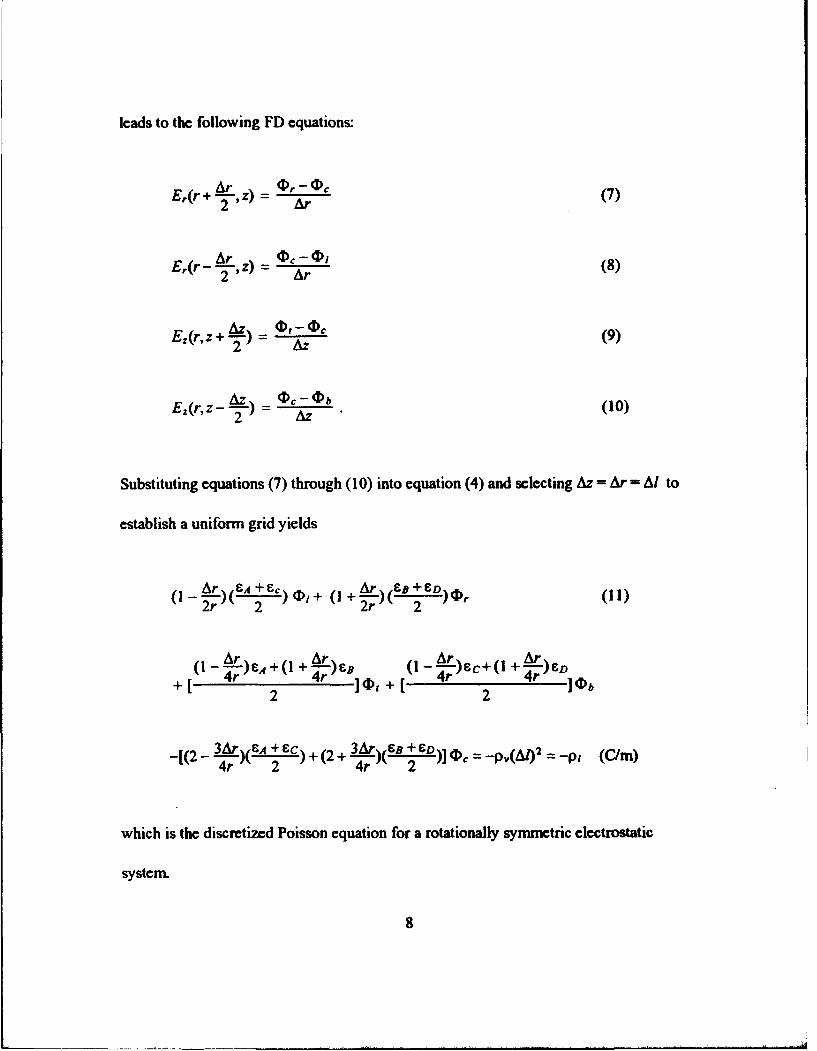
leads to the following FD equations:
(7)
(8)
E llz) <1>,- <l>c z(r,z+T = llz (9)
(10)
Substituting equations (7) through (1 0) into equation ( 4) and selecting llz =~=Ill to
establish a uniform grid yields
(11)
which is the discretizcd Poisson equation for a rotationally symmetric electrostatic
system
8

--------------------------------------------------------------------------
The development of the magnetostatic Poisson equation also begins with the
elementary volume in cylindrical coordinates. A cross section of the elementary volume is
shown in Figure 3.
At
Axis of Symmetry
Figure 3. Magnetostatic Elementary Volume
In this figure, the current (I) and the magnetic vector potentials (A,. A,, A,, Ab and AJ
are all in the e direction. This allows the magnetic vector potential to be treated as a
scalar. Using this fact along with the integral form of Ampere's Law. a discretized form of
Ampere's Law can be developed. Ampere's Law relates the magnetic field around a
9
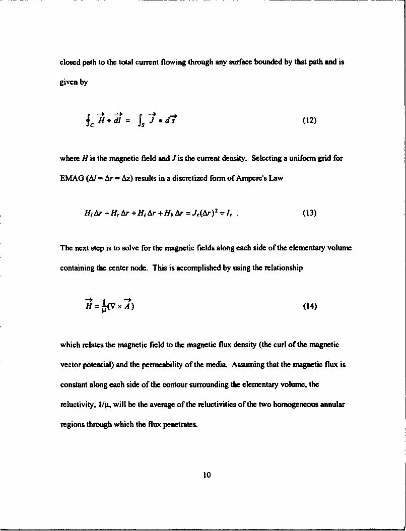
closed path to the total current flowing through any surface bounded by that path and is
given by
f -+-+ I-+,_. c H • dl = s J • d s (12)
when: His the magnetic f~eld and J is the current density. Selecting a uniform grid for
EMAG (ll/ = llr = llz) n:sults in a discn:tized form of Ampen:'s Law
(13)
The next step is to solve for the magnetic faclds along each side of the elementary volume
containing the center node. This is accomplished by using the n:lationship
-+ I -+ H= Jl(Vx A) (14)
which n:latcs the magnetic facld to the magnetic flux density (the curl of the magnetic
vector potential) and the permeability of the media. Assuming that the magnetic flux is
constant along each side of the contour surrounding the elementary volume, the
n:luctivity, 1/Jl, will be the average of the n:luctivities of the two homogeneous annular
n:gions through which the flux penetrates.
10

Using this value for reluctivity along with the: definition of curl in cylindrical coordinate
systems and the: fact that all of the: magnetic vector potentials are exclusively in thee
direction, equation (14) becomes
(IS)
where r is the center node's radial distance from the axis of rotation. Applying cq, ..• ton
(IS) to all four sides of the volume results in the following four FD equations for the
magnetic fields shown in Figure 3:
(16)
(17)
(18)
(19)
11

Substituting equations (16) through (19) into equation (13) yields
I I I I I I -[-(-+-)]A,-[-(-+-)] Ab= I 2 J.l..4 J.lB 2 J.lc J.lD c (Amps).
Equation (20) is the discrctizcd magnetostatic Poisson equation which ~elates the
potential of the center node to the potential of its four nearest neighboring nodes and the
currcnt through the center node. Although equations (II) and (20) look very difTercnt
from one another, they both tend toward the z-invariant Poisson equations used in
EMAG as r tends toward infinity. This fact is the basis for the approach used to modify
the EMAG code prcscntcd in the next section.
12

B. IMPLEMENTATION OF DISCRETE POISSON'S EQUATION IN EMAG l.O
In order to solve rotationally symmetric problems, the original version ofEMAO
needed to be modifted in three ways. First, in the equation solver subprograms, code
needed to be added which applied the Poisson equations derived in the previous section.
These types of modifications are the subject of this section. The second set of
modifications, to be discussed in Chapter Ill, involved the usc of rotational symmetry
equations to develop the TOT boundary data. The third set of modifications involved
addition of code to allow EMAO 2.0 users to choose between z-invariant and rotationally
synunctric systems. This last set if modifications will not be discussed except in the
context of how EMAO 2.0 is used. All modifaed EMAO subprograms can be found in
Appendix A.
The original version ofEMAO uses two different methods for calculating the
potentials across the computational grid. The first method, intended for solving coarse
( 17 x 17) grid problems, utilizes a system matrix containing all information about media
and the TOT boundary. This system matrix is generated by the MA TLAB script file
makesys2.m. The script file matsolve.m then applies the user spccifaed source
information and solves the system of equations using matrix operations. To modify the
coarse solver for rotational symmetry, equations (11) and (20) were used. Specifically,
the factors in these equations which weight the media parameters based on the center
node's relative distance from the axis of symmetry (such as ( 1 - t)) were inserted into
13

duplicates of the z-invariant equations. These equations~ used instead of the
z-invariant set when the user specifiCs that the problem to be solved has rotational
symmetry. The system matrix approach was not used in the original version ofEMAG in
solving fine ( S 1 x S 1) grid problems, because of the large size of a fine grid system matrix
and the fact that the sparse matrix tools were not yet included in MATLAB. For a fine
grid of this size, the system matrix would contain nearly 6.8 million elements and require
54 megabytes of memory if stored as a full matrix [Ref. 1]. As a result, a second, more
memory conservative solution approach was utilized.
The method originally used in EMAG for solving fine grid problems was a Jacobi
iterative solver. ( The reasons for choosing a Jacobi solver ~ detailed in Reference 1.)
This solver is contained in the MA TLAB script file itersoln.m. The Jacobi solver can
utilize saved results from previous problems, the results of the coarse solver or a default
set of potentials (zero except where known a priori) as the starting point for its iterations.
The EMAG user specifics a desired percent error at which to stop iterating the solution.
The computational time required to solve a problem using this approach increases with
the degree of accuracy required. Because the modifications leading to EMAG 2.0 were
accomplished using MA TLAB 4.0, sparse matrix operations were utilized in the system
matrix solver to allow it to be used for both coarse and fine grid solutions. The Jacobi
solver however, was not eliminated since it has the useful advantage that it can usc
previous solutions as the starting point for its iterations, thereby increasing its speed of
14

convergence to the solution. For example, by using the coarse grid solution as a starting
point for a fine grid calculation, the iterative solver can often run faster than the system
matrix solver with an estimated error less than I%. The system matrix approach, which
n:quin:s the same computational time n:gardless of the problel'llt cannot take advantage
of a pn:vious solution, but generally runs faster than the Jacobi solver without an
accurate starting set of potentials. Accordingly, in EMAG 2.0 the user has a choice of
using either the Jacobi solver or the system matrix solver when solving a problem on the
fine grid. Fine grid problems using the system matrix approach an: solved using the
matsolvf.m and makesysf.m script files. The iterative solver in itersoln.m has been
modified to include the Poisson equations for rotational symmetry. Modifications to
itersoln.m wen: similar to those made to makesys.m in that the rotational symmetry
unique terms wen: applied as factors weighting the media parameter terms.
When EMAG 2.0 users desin: to solve a rotationally symmetric problem, they simply
answer "y" (or "Y") to the question "Do you want to solve a rotationally symmetric
system?" in the "New Domain Region" selection part of the EMAG session. Once this
choice is made, EMAG 2.0 remains in the rotational symmetry mode until a new domain
n:gion is n:qucsted. As a n:minder that EMAG is in the rotational symmetry mode, a
border around the computational grid is plotted in red. This border is white in the
z-invariant mode. The user then defines cells of media and sources on the computational
grid in the same manner as in the z-invariant case except that only the right half of the
IS

cross section of the system is visible. For problems in electrostatics, the axis of
symmetry is parallel and one half of an inter-nodal distance (AI) to the left of the left
side of the computational grid. For magnctostatic problems, the axis of symmetry is
parallel and a whole inter-nodal distance to the left. These arrangements take advantage
of symmetry, maximize the useful input area of the computational grid, and eliminate the
mirror images that would result if the axes of symmetry had been chosen to be in the
center of the computational grid. They also allow reuse of the drawing routines used for
z-invariant systems. A sample electrostatic problem on the EMAG 2.0 rotational
symmetry computational grid is shown in Figure 4.
Inner Conductor l Axis of Symmetry
Border
i Axis of Symmetry
Figure 4. Section of Coaxial Cable on Computational Grid
16

Figure 4 depicts the right half cross section of a short segment of a coaxial cable as it
would appear on the EMAG 2.0 computational grid. (If the user had not requested a
rotationally symmetric problem, this same picture would represent a parallel plate
capacitor extending infinitely into and out of the computational grid along the z-axis.)
In addition to the changes to the system solver programs listed above, EMAG's
subroutines required several other modifications to accommodate rotational symmetry.
First, the subroutines cefield.m andfefleld.m, which plot the electric or magnetic fields
for the coarse and fine grids respectively, were modified so that the magnetic fteld would
be calculated using the definition of curl in cylindrical coordinates. Next, the enclosed
charge calculation subprogram, q_calc.m, which performs a flux integral, was modifJCd
to account for the fact that the area of the faces of the elementary volume arc functions of
the volume's distance from the axis of rotation. This modification results in the charge
enclosed in a user specified area of the rotationally symmetric computational grid being
expressed as total charge (in Coulombs) instead of charge per unit length
(Coulombs/meter) as it is in the z-invariant case. The last modification was applied to
the enclosed current subroutine i_calc.m. This subroutine was modified so that the
enclosed current for rotationally symmetric systems is calculated using the definition of
curl in cylindrical coordinates. The modified versions of all the above subroutines arc
included in Appendix A.
17

III. MODELING OF OPEN BOUNDARY
A. THEORY OF TRANSPARENT GRID TERMINATION (TGT)
In order to quickly and accurately solve open boundary problems, EMAG uses a
technique called Transparent Grid Termination (TGT) to simulate the existence of a zero
potential, Dirichlet boundary far away from the user defined problem on the
computational grid. Using the known zero potential on the Dirichlet boundary and
defining all space outside EMAG's computational grid to be source free and
homogeneous, a very large system of Poisson equations involving the nodes inside the
Dirichlet boundary is panially solved in advance. The end result of this process is a
system of equations which relate the potentials of the nodes on the first layer outside the
computational grid (called the TGT boundary) to all of the nodes just inside of this layer,
given that there exists a distant boundary of zero potential. These equations arc stored in
the fonn of a matrix (called the TGT matrix) which, once calculated, replaces the many
concentric layers of nodes in the homogeneous, source free region between the
computational grid and the distant Dirichlet boundary.
Since this original "buffer" zone of nodes was defined to be homogeneous and source
free, this TGT matrix does not change from problem to problem and in no way depends
on what may be defined within the computational grid for any particular problem. As
such, the TGT matrix is stored and reused over and over to solve any user defined
18

problem quickly. Since the TGT boundary relationships arc calculated by partially
solving the larger physical system with a Dirichlet boundary, TGT provides exactly the
same solution as would be obtained by solving the user defined problem with a distant
homogeneous Dirichlet boundary. However "solving through" this unchanging buffer
zone once and storing the results eliminates repetitive and time consuming computations.
Solving the whole open boundary problem would require several hours on even the
fastest PC. The vast majority of this time would be spent solving through the buffer zone
which docs not change from problem to problem. TGT simply allows one to devote this
time only once in the calculation of the TGT matrix and then to use the results of this
partially solved system for different problems. [Ref. 1]
Figures 5 and 6 illustrate the relationships between the computational grid and the
Dirichlet boundary for z-invariant and rotationally symmetric systems respectively.
The arrows in these two figures show how each node on the TGT boundary is globally
related to every node on the outer layer of the computational grid and the Dirichlet
boundary while each node on the computational grid is related only locally to its four
nearest neighbors [Ref. 2]. Notice that unlike the z-invariant computational grid
(Figure 5), the rotationally symmetric computational grid (Figure 6) has a distant
Dirichlet boundary on only three sides. The left side of the rotationally symmetric
computational grid for electrostatic systems is adjacent to the axis of symmetry and as a
result, has a Neuman boundary of zero gradient to its left. The axis of symmetry for
19

oooo 0
0 0
0
0
0
0 0
.. oooo 0
0
0 0
0 0
0 0
o e .. e .. e ....•..•... e .. e o O TGT boundary 0
0 distant Dirichlet boundary 0 0···0 00····0·0 ·0 00··00··0·0
Figure 5. z - Invariant System
,,....-----. Axis of Rotation for Electrostatics
Axis of Rotation for Magnetostatics
... o.o.o .. o 0 0 C)
0 0 0 6 C)
0 0
• distant Dirichlet boundary O 0····0··0···0···0···0···0···0···0
Figure 6. Rotationally Symmetric System
20

the magnetostatic rotationally symmetric system is placed on the left side of the TOT
boundary and is a homogeneous Dirichlet boundary. The reason for the different
placements of the rotationally symmetric electrostatic and magnetostatic computational
grids is that for magnetostatic systems with only e directed components of magnetic
vector potential, the potential is known to be zero on the axis of rotation. In contrast, for
the electrostatic system, it is the gradient of the electric scalar potential that is zero on the
axis of rotation. Different grid placements, therefore, take advantage of these known
facts in establishing the boundary conditions. As shown in Figures 5 and 6, EMAO
always uses a square computational grid and the TOT boundary is a layer of nodes one
inter-nodal distance outward from the last layer of the computational grid. This TOT
boundary contains all information about i:he distan~ Dirichlet boundary required to solve
any problem drawn by a user on the computational grid with the same accuracy as
solving the much larger problem within the distant Dirichlet boundary. With the T'"'!T
boundary matrix calculated in advance, EMAO only needs to solve the sparse system of
equations depicted by the topology map of Figure 7. [Ref. 2]
21

j1(D) E :I c
-11500 0 c
2500
Topology Map
'
'· ~--~------~------~ 0 500 1(0) 1500 Dll 2500
node number
Figure 7. EMAG System Sparsity Pattern
.J
Spiral Node LIWIID&
Figure 7 is a mapping of the non-zero clements in the matrix which relates the nodes
on the computational grid and the TGT boundary to one another. A spiral node labeling
pattern is used, starting from the upper left node on the TGT boundary and spiraling
clockwise inward to the center of the computational grid The main "diagonal" is three
clements wide and represents the relationship between a node and its nearest neighboring
nodes on its right and left. These relationships arc derived using the discretizcd Poisson's
equations, equations (II) or (20). The upper diagonal represents the tcnns which relate
each node to its neighboring node immediately inward, toward the center. The lower
22

diagonal represents the tenns which relate each node to its neighbor outward, away from
the center. The dense square area in the upper left corner of the map represents the TGT
matrix. It is this densely packed matrix which relates the potentials of the nodes on the
TGT boundary to the nodes on the outer edge of the computational grid wven the fact
that there exists a distant Dirichlet boundm of zero potentia). Whereas the diagonals
represent local relationships between a node and its neighbors, the TGT matrix relates
each node on the TGT boundary globally to all the nodes on the outer edge of the
computational grid. The spiral numbering scheme is used in order that the TGT matrix be
densely packed with no non-zero elements, thereby minimizing its size. The next two
sections of this chapter will present two different approaches to calculating the TGT
matrix. The final section of this chapter will compare these techniques and present the
results of research into the optimization ofTGT. [Ref. 2]
23
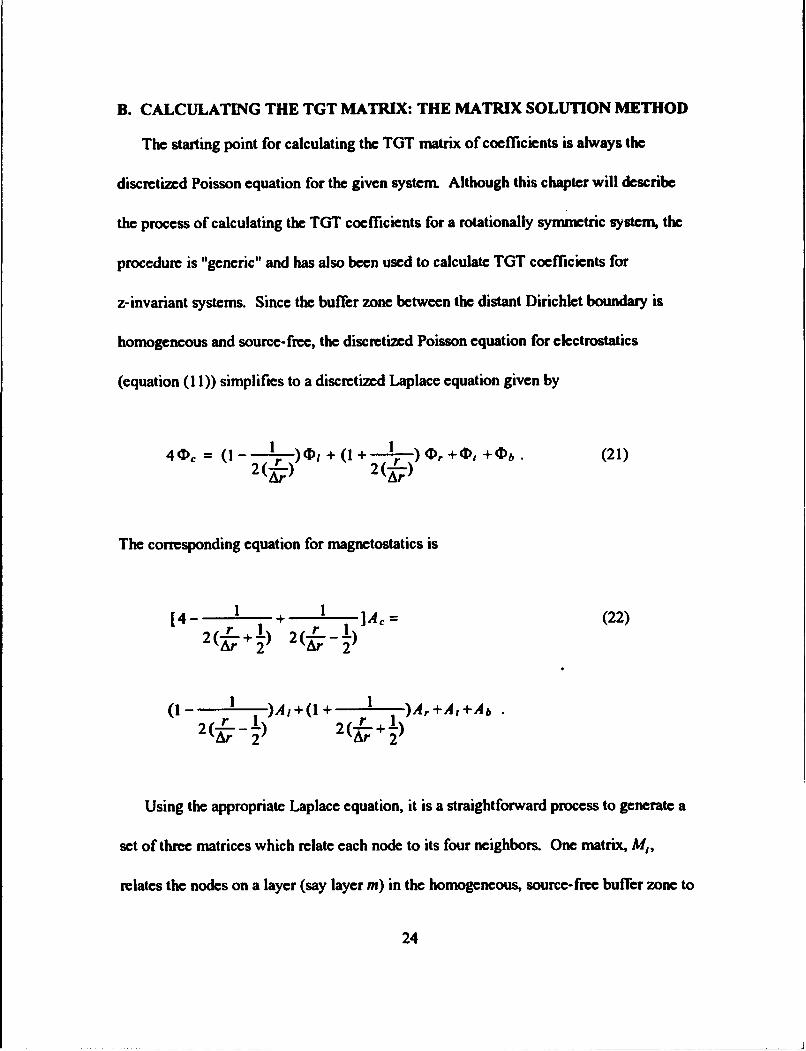
B. CALCULATING THE TGT MATRIX: THE MATRIX SOLUTION METHOD
The starting point for calculating the TOT matrix of coefficients is always the
discretized Poisson equation for the given system Although this chapter will describe
the process of calculating the TOT coefficients for a rotationally symmetric system, the
procedure is "generic" and has also been used to calculate TOT coefficients for
z-invariant systems. Since the buffer zone between the distant Dirichlet boundary is
homogeneous and source-free, the discretized Poisson equation for electrostatics
(equation (11)) simplifies to a discretized Laplace equation given by
(21)
The corresponding equation for magnetostatics is
(22)
Using the appropriate Laplace equation, it is a straightforward process to generate a
set of three matrices which relate each node to its four neighbors. One matrix, M1,
relates the nodes on a layer (say layer m) in the homogeneous, source-free buffer zone to
24
--~---- ~~ J

their neighbors on the next layer of nodes outward toward the Dirichlet boundary (say
layer 1). The second matrix, M,. , relates nodes on layer m to the nodes on the next layer
inward toward the computational grid (layer n). The third matrix, M., relates the nodes
on a layer to themselves and their two neighbors on the same layer. Because these
matrices have a discernible pattern, and arc functions of the computational grid size and
the relative size of the m-th layer of nodes, they can_ be generated algorithmically.
Functions for creating these matrices via MA TLAB arc included in Appendix B. The
three functions makem/c.m, makemnc.m and makemmc.m produce the M1• M,. and M.
matrices respectively, for rotationally symmetric electrostatic systems. The functions
magmlc.m, magmnc.m and magmmc.m perfonn the same functions for magnetostatic
rotationally symmetric systems. The two input parameters for these functions are the
number of nodes on a side of the desired square computational grid and the number of
nodes on the right or left side of the m-th layer of nodes.
As shown in Figure 6, layers of nodes outside the computational grid are defined to
have only three sides for a rotationally symmetric system. Symmetry makes it
unnecessary to calculate the TGT coefficients for the left side of the TGT boundary. For
electrostatic systems, these nodes arc known to be at the same potential as their "mirror
images" across the axis of rotation (Neuman boundary condition). The upper left and
lower left nodes on the TGT boundary have the same TGT coefficients as their image
nodes across the axis of rotation. The remaining nodes on the left side of the TGT
25

boundary have the same potential as their images and therefore have a single TOT
coefficient equal to one, which relates them only to their image node on the
computational grid. Figure 8 illustrates these relationships. In this fi~, the gray nodes
arc TOT boundary nodes and the black ones belong to the computational grid.
v Share Same OJeffrcients
.;--r • •• •
One 1. TGTS Coefficient •
Each
• • • ·~Axis of &Jtation
• • • • • •
·~· •
• • • •
Share Same OJefficients
Figure 8. Left Side ofTGT Boundary for Electrostatics
For magnctostatic systems, the potentials on the axis of rotation arc known to be zero so
the left side of TOT boundary has been placed on the axis and all of the corresponding
coefficients have been set to zero (local Dirichlet boundary condition).
26

Samples of the output of each of these functions and their MA TLAB script file listings
arc in Appendix B. The samples were generated for the first layer of nodes outside a
three by three node computational grid such as shown in Figure 8. Output from these
functions arc m by x matrices (x=l,m or n) for which the rows represent the nodes on the
m-th layer and arc numbered in a clockwise fashion starting with the node in the upper
left corner of the layer. The columns represent the nodes on the /, m or nth layer and arc
numbered in the same manner. As can be seen from the sample outputs for this small
computational grid, the matrices can get to be quite large. Fortunately, they arc always
very sparse. Also inc1udcd in Appendix B arc the three functions makeml.m, makemn.m
and makemm.m which generate the M1, M,. and M. matrices for z-invariant systems along
with samples of their output. Note that for z-invariant systems, these matrices arc not
functions of the inner grid size. The reason for this is that the layers of nodes outside the
computational grid arc concentric squares for this coordinate system. For rotationally
symmetric systems, these layers of nodes arc rectangular in shape and missing a left side.
Further, it is important to note that there is no need to have different sets of programs to
generate TOT coefficients for z-invariant electrostatic and magnetostatic systems since
the z-invariant Laplace equations for electrostatics and magnetostatics arc identical.
The process of solving for the TGT coefficients begins with a vector , Ia>, which
represents the potentials of the nodes on the Dirichlet boundary (layer a) and the node
relationship matrices discussed above for the next layer inward (layer b ).
27

The discrctized Laplace's equation in matrix fonn is
(23)
where lb> and lc> represent the potentials on the next two layers inward, b and c
respectively. Continuing one layer inward leads to
(24)
Given that la>=O for a layer with zero potential, equations (23) and (24) can be
combined and solved to find lc>, the potentials of the nodes on layer c, in tenns of the
nodes on the next layer inward. This solution is given by
(25)
Since this solution docs not depend on the potentials of nodes on layers a or b , these
layers have been effectively eliminated from the problem. To calculate the TOT
coefficients, this process of layer elimination is continued inward towards the
computational grid Since the subsequent expressions grow in length with every
elimination, a special "termination" matrix can be defined for each node layer.
28

To simplify notation, define
(26)
and
(27)
as the termination matrices for layers band c respectively. [Ref. 2]
In general, the expression which relates the nodes on a layer to the nodes on the next
layer inward is given by
lm > =(f ~-1 M, In> (28)
where the generic termination matrix, r,' can be calculated iteratively by
(29)
When this elimination process is continued inward until the TGT boundary layer is
reached, the TGT coefficients arc obtained by
TGT= (f "')-1M,. (30)
29

The MA TLAB script files , coefgenc.m and coefmagc.m, used in calculating the TGT
coefficients for rotationally symmetric electrostatic and magnctostatic systems
respectively, can be found in Appendix B. These programs calculate the TGT
coefficients for three sides of the TGT boundary using the algorithm discussed above.
They then add the remaining terms for the fourth side based on symmetry and either
known potentials or known gradients of potential. The last program contained in
Appendix B is the TGT coefficient generating script file for z-invariant systems,
coefgen.m. [Ref. 2]
30

C. CALCULATING THE TGT MATRIX: THE MONTE CARLO METHOD
The Monte Carlo Method (MCM) is a technique used to approximately solve a
mathematical problem through the use of a probabilistic model [Ref. 3: p. 73]. To use
the MCM to solve for TOT coefficients, a MA TLAB algorithm was developed to
"release" a faxed number of"random walkers" from a node on the TOT boundary. The
direction in which each of these walkers travel is determined and assigned based on the
outcome of a random number generator and the relationship between nodal potentials
given by the discretized Laplace equation for the appropriate system For a z-invariant
system, random walkers arc assigned an equal 25% probability of going up, down, right
or left. This is because the pf)tential of a node in the homogeneous source-free buffer
zone between the computational grid and the defined far Dirichlet boundary is 25% of
the sum ofthe potentials of each of its four neighbors (above, below, to the right and
left). For rotationally symmetric electrostatic systems, however, the "contributions" of
the right and left neighboring nodes are weighted by the (1- 1, ) and (I+ 1, ) 2(Ar) 2(Ar)
terms of equation (21 ), repeated below for convenience
(31)
31

Similarly, the weighting factors for the rotationally symmetric magnctostatic system
come from equation (22), repeated below
(32)
As can be seen in equation (32), the potential of the center node is also weighted for
magnetostatics.
After every step, each random walker is given a new direction based on a new random
number and the walker's current location. The walkers continue their "journey" until
they land on the computational grid or the distant Dirichlet boundary. If they land on the
Dirichlet boundary, they are eliminated as if to be "nullified" by the zero potential of the
boundary nodes. If they land on the computational grid, a counter which counts the
number of walkers to land on that node is incremented by one and again the walker is
eliminated. Once all of the walkers have been eliminated, the final count of walkers
arriving at each node on the computational grid is divided by the number of walkers
originally released. The end result is a set of coefficients which relate the original walker
release node to each of the nodes on the outside edge of the computational grid This set
is a row in the TGT matrix. The MA TLAB functions which perform this algorithm are

contained in Appendix C. The functionfncylwlk.m is used for rotationally symmetric
electrostatic systems whilcfnrctwlk.m is used for z-invariant systems. The programs
cylcoff.m and rctcoff.m, also in Appendix C, call these functions once for each node on
the TGT boundary and assemble the data into the TGT matrix for rotationally symmetric
and z-invariant systems respectively. As in the case of the matrix solution method, the
TGT coefficients for the nodes on the left side of the TGT boundary in a rotationally
symmetric system arc derived using symmetry. This is done not just to improve
efficiency but out of necessity since a walker on the left edge of the buffer zone is
exactly ~ away from the axis of rotation and by the electrostatic Laplace equation has
zero probability of stepping to the left. Accordingly, no walker can ever land on the left
side of the computational grid and the TGT relationships can only be determined by
using the symmetry of the system For reasons discussed in the next section, TGT
coefficients for rotationally symmetric magnetostatic systems were not calculated using
the MCM approach, although this could be easily accomplished with only slight
modification to rctcoff.m andfnrctwlk.m.
33

D. COMPARISON OF TGT METHODS
Each of the two methods for calculating TGT coefficients discussed previously have
advantages and disadvantages. The greatest advantage of the Matrix Solution Method is
its accuracy. As discussed in the first section of this chapter, TGT provides the same
accuracy as solving the whole open boundary problem without TGT. This is because the
matrix solution method uses Poisson's equation to solve for the TGT coefficients just as it
would be used to solve the whole open boundary problem The Monte Carlo Method
(MCM) approach however, is only based on the Poisson equation and will always be
subject to an amount of random "noise". The MCM approach gencraJJy makes TGT less
accurate than solving the whole open boundary problem. For this reason, the TGT
coefficients used in EMAG 2.0 were calculated using the matrix solution method.
Insufficient accuracy, however, docs not necessarily eliminate the MCM approach
because its accuracy is improved by using a very large number of walkers. This
increases computation time, but parallel processing can be used to recover this time as a
result of the parallel nature of the problem (i.e., the independence of random walk
outcomes for different walkers). Further, the MCM approach has the advantage that it
allows the user to exchange run time for computer memory. The user can release large
sets of walkers a few times to maximize the usc of available memory and improve speed
of computation, or the user can choose to release only a very few walkers many times
thereby increasing computation time but using little memory. In this way, the user can
34

select a set of walkers of a size which either maximizes or minimizes the usc of memory.
The number of walkers can effectively be increased by running the program a number of
times and averaging the results. In this way, there is no limitation on either the number
of walkers or the distance to the Dirichlet boundary except for the CPU time. This can
be a distinct advantage over the matrix solution method which is primarily limited by the
available memory. The process of layer elimination for the matrix method, requires that
the CPU have enough available memory to invert and store a square matrix with
dimensions equal to the number of nodes on the first layer to be eliminated Although
sparse matrix tools available in MA TLAB help, the inverse of a sparse matrix is
generally not sparse. A memory limitation can only be alleviated by moving the
Dirichlet boundary closer to the computational grid.
35

E. TGT OPTIMIZATION
This section summarizes the research into optimization ofTGT. The questions to be
answered concerning optimization are:
1. Given a computational grid size, is there an optimum distance at which to put the
Dirichlet boundary?
2. Using the Monte Carlo Method and the optimum boundaly distance from above,
how many random walkers are required to produce accurate TGT coefficients?
3. Given the answers to the first two questions, how do speed of computation and
memory requirements compare between the two TOT methods?
Optimization of TOT begins with answering the first of these questions. This answer
is important because the first step in using TOT is deciding how far away to place the
Dirichlet boundary. The result of this decision controls the speed of calculation and
memory required as well as the accuracy of calculations within the TGT boundary. In
calculating the TOT matrix for use in the original version ofEMAO, this decision was
made based on the memory limitations of the computer used to calculate the TOT
coefficients (a HP-700 series UNIX workstation). As the result, the Dirichlet boundary
was established for the "fine" grid to be 803 by 803 nodes or 376 layers away from the
computational grid. In order to maintain the same ratio between the boundary and
computational grid size, the boundary for the "coarse" grid was made 267 by 267 nodes
or 125 )ayers away from the computational grid [Ref. 1]. The following paragraphs
36

describe the research conducted to determine the optimum boundary location for a given
computational grid. This research w~ conducted using a z-invariant system since the
z-invariant computational grid has a distant Dirichlet boundary on all four sides and the
layers of nodes in the buffer zone between the boundary and the computational grid arc
concentric squares. However, it has been verified that the results apply to rotationally
symmetric systems as well.
Ideally, if the EMAG computational grid were actually surrounded by free space, the
TGT coefficients relating a node on the TGT boundary to the nodes on the outer edge of
the computational grid would always sum to unity. In the language of the MCM
approach, this is because the walkers would have no outer boundary to land on and
would all eventually land somewhere along the edge of the computational grid. As a
result of this property, a measure of the quality of the TGT matrix can be defined as
Lq; Qror=-n- , q;=LCn (33)
where q; is the sum of all the coefficients (c,.) relating the i-th node on the TGT boundary
to the nodes on the edge of the computational grid and n is the number of nodes on the
TGT boundary [Ref. 4]. For a computational grid in infinite free space, Q would be
equal to one. Now, if Q was the only factor governing the quality of the TGT
coefficients, the original approach of placing the Dirichlet boundary as far away from the
37

computational grid as possible would be the best solution. However, thcR: is a fmite
limit at which the size of the Dirichlet boundary becomes so large in comparison to the
size of the computational grid, that moving the boundary further away yields diminishing
R:tums. In tenns of the MCM approach, this phenomenon can be described as walkers
being moR: likely to land on a very large but distant Dirichlet boundary than a R:latively
small computational grid simply because of the vast diffeR:nce in their sizes. As a
specific example, an 11 by 11 computational grid would have 40 nodes on its outer edge.
A 21 by 21 node Dirichlet boundary layer would be only five layers away but would
already have 80 nodes or twice as many as aR: on the edge of the 11 by 11 computational
grid. The size of the Dirichlet boundary grows by eight nodes for every layer it is moved
away from the computational grid.
In order to determine the R:lationship between the size of the computational grid and
the optimum size of the Dirichlet boundary, the matrix solution algorithms for
calculating TGT coefficients described in section B of this chapter weR: used. Early
attempts at this involved fixing the computational grid size and moving the Dirichlet
boundary further away one layer at a time while looking for a point at which the R:lative
change in Q between successive computations was less than 0.1 %. During this process,
it was noticed that for a fixed Dirichlet boundary size, choosing successively smaller
computational grids would eventually R:sult in a maximum value for Q after which it
dropped rapidly. This R:sult was contrary to the expectation that moR: layers of nodes
38

~-------------------------------------------------------------------------
between the boundary and the computational grid would always ~suit in higher Q's.
Through investigation of this phenomenon, it was discovered that for a given Dirichlet
boundary size there is a computational grid size which maximizes Q but that the convene
of this is not true. This observation led to a "~venc" approach of starting with a known
Dirichlet boundary size and searching for the ideal computational grid size. To this end,
a Dirichlet boundary size was chosen and the row elimination process involved in
calculating the TOT coefficients begun. As each row was eliminated, a new set of TOT
coefficients was generated as if the dcsi~d TOT boundary had been ~ached. The Q
factor for this set of TOT coefficients was then calculated and stored. This process was
continued until the inner-most layer was reached (a 3 by 3 layer of nodes). The stored
values for Q were then plotted versus the dimension of the layer at which they were
calculated. The resulting curve ~presented the Q factor trend for a fixed Dirichlet
boundary size as the computational grid was decreased in size. The Q curves ~suiting
from using Dirichlet boundary sizes of 51 by 51, 1 01 by 101 , 151 by 151 and 201 by
201 ~shown in Figure 9.
39
Q

Figure 9. Boundary Curves: Q-Factor Trend
The starred points on each of the curves in Figure 9 represent the TGT boundary size
(and therefore the computational grid size) which corresponds to the maximum value of
Q. These curves illustrate that although moving the boundary further away will always
increase the Q for a fiXed computational grid size, this computational grid size will
eventually fall on the left hand side of the boundary curve when: Q drops off. Choosing
computational grid sizes which correspond to the maxima on each of these curves results
in a set ofTGT coefficients that most effectively match the resolution of the grid To put
it another way, although moving the Dirichlet boundary further away always improves
40

the TGT coefficients, there is a point at which the resolution of the grid becomes the
limiting factor in solution accuracy and improving TGT is no longer beneficial.
To determine the function which relates the optimum computational grid size to the
Dirichlet boundary size, boundary curves were generated for 9S Dirichlet boundary sizes
ranging from 11 by 11 to 201 by 201. The resulting computational grid sizes were
plotted against their corresponding boundary sizes as shown in Figure 10.
,J' .•... /
0o 10 20 30 40 50 60 70 Compulebonll Gncl OmenSIOII
Figure 10. Boundary to Grid Size Relationship
Figure 10 shows that there is a linear relationship between the Dirichlet boundary size
and the corresponding optimum computational grid Figure 11 is a plot of the ratios of
the sizes of the data pairs plotted in Figure I 0.
41

Figure II. Convergence of Data
Figure II shows that the ratio of Dirichlet boundary size to computational grid size
converges to a value of2.879. As a result, the Dirichlet boundary size to be used with a
given computational grid can be calculated directly by multiplying the desired grid size
by 2.879 and then rounding to the nearest odd integer if the computational grid is of odd
dimension or to the nearest even integer if it is of even dimension.
Once the relationship between the boundary and the computational grid sizes was
dctermir.ed, the number of MCM random wallcen required to accurately solve the TOT
problem could be evaluated To accomplish this, sets of TOT coefficients wen:
42

generated using varying numbers of walkers for a fiXed computational grid size and a
distant Dirichlet boundary established from the condition given above. These TGT
coefficients wen: then compared to the matrix method TGT coefficients to dctennine a
tenn-by-term error, &t, given by
(34)
where St is the k-th, matrix method TGT coefficient and s t is the k-th coefficient
generated by the MCM approach. A root-mean-square (RMS) error was then
determined for the MCM coefficients by
Error.,..= J~<;;>' (35)
where N is the number of coefficients in the set. This result was then used to form an
error-to-data ratio by using an RMS measure of the matrix solution TGT coefficient set
given by
(36)
43

and the relationship
(37)
Using this measure of accuracy, data was collected over a wide range of numbers of
walkers. The results of many equal-sm:d sets of walkers were then used to produce a
mean value and standard deviation for the error between trials associated with using a
particular number of walkers. The lower curve in figure 12 depicts the mean
error-to-data ratio for sets of MCM walkers using an II x II computational grid Curves
for one and three standard deviations above the mean are also shown.
Accl.lracy ota.ICM tJr f fxf f Comc~~Jtdanll Grid -15,.----........ -------------.
·20
i:-25 \ .s • ~~ '\....., -1 ,:-._ .. __ c5..s5 \ . ....... -!l , '-. '-·--....__ m + 3o IS '· -..._ ~-~-40 .... ..... __ ....__ w ......... ---- ;;; + 0 ... __ _ c ............ ---......_ 1-45 --- --·--~-. 2 -------- ··-----...... iii --------~ ...
~~~---~0~.5~---~1----~1~5----~2 IIUilblr o1 Rllndom Wllters x 10s
figure 12. Error vs. Number of Walkers
44

The Central Limit Theorem states that the sum of many statistically independent random
variables approaches a Gaussian random variable. The number of walkers that will yield
a set ofTGT coefficients with a given decibel error 99.7% (m+Jo) of the time, can
therefore be chosen by using the upper standard deviation Jine in Figure 12 [Ref. S:
pp. 425-430]. To achieve -40dB error with this level of success for an II x II
computational grid would require approximately I.S x 105 walkers. To achieve this
same error level but with 68.3% reliability, the lower standard deviation line (m+o)
indicates that only about S x I 04 walkers would be required. This type of analysis has
been conducted for grid sizes smaller and larger than 11 x II and it has been observed
that the required number of walkers actually diminishes slightly with increasing grid size
(at least up to 51 x 51, the size ofEMAG's "fine" grid). This is due to the fact that for
larger computational grids a greater number of the TGT coefficients are very small and
contribute little to the RMS values for the data and error. An approximation for the m+a
curve is given by the equation:
X Error -106 (-)dB= 40e -80 Lata
(38)
where xis the number of walkers released from each node on the TGT boundary. This
approximation is only valid for numbers of walkers greater than about 50,000 but gives
an indication of how many walkers would be required to achieve accuracies greater than
45

shown in Figure 12. Using this approximation, about 700,000 walkers would be ~ired
to achieve a -60 dB error to data ratio with 68.3% reliability.
With the fint two optimization questions answered, the computational speed and
memory requirements for the two TGT coefficient generation methods were compared.
This comparison was made by calculating a set ofTGT coefficients for EMAG's "coarse"
and "fmc" computational grid sizes. The number of MCM walkers was chosen to
provide a -40dB error at a 68.3% level of reliability (m+<J). Table 1 contains the results
of this comparison. The computational times were obtained by calculating TGT
coefficients on an IBM compatible 486 class PC. The memory requirements arc
estimates based only on the sizes of the matrices stored by each coefficient generating
program and do not account for any of the MA TLAB overhead memory needed for the
inversion of the sparse matrices, etc.
TABLE 1: COMPARISON OFTGT METHODS
17 X 17 S1 x SI
Memory(KB) Time (sec) Memory(KB) Time (sec)
Matrix 271 100 2,700 6,520 Method
MCMwith 400 29,700 400 217,000 Sx1 04 Walkers
46

As can be seen in Table 1, the matrix solution method is considerably faster than the
MCM approach. It should also be noted however, that the mernol)' requirements of the
MCM approach do not change with increasing grid size while the memol)' requirements
for the matrix solution method grow rapidly. Furthennorc, although computational times
for the matrix method arc much shorter than the MCM times, they also grow at a much
faster rate than the MCM times. Finally, it needs to be noted that the MCM coefficient
generating algorithm used here docs not take advantage of the symmeli)' of the system
For z-invariant systems, one could calculate TGT coefficients for one-eighth of the nodes
on the TGT boundal)' and then usc symmetcy to completely fi)) the TGT matrix. Such an
approach would theoretically cut the MCM times by a factor of eight. Similarly, the
rotationally symmetric MCM coefficient generation time can be reduced, but only by a
factor of two. Furthennorc, only three-quarters as many coefficients need to be
generated using MCM for a rotationally symmetric system (the left side coefficients arc
already obtained by using the symmeli)' about the axis of rotation) resulting in a
computational time of about three-eighths of the value listed in the table.
As shown in this section, there is a choice of method by which the TGT boundal)'
matrix can be calculated. Although the matrix solution method is the most desirable
approach when using sequential computers to calculate TGT coefficients for EMAG's
current computational grid sizes, the MCM approach can take advantage of parallel
processing capabilities. This is because the paths taken by the individual walkers arc
47

statistically independent. The same statistical independence holds even for consecutive
steps taken by a single walker. Using a parallel MCM algorithm, a massively parallel
computer (l 024 processors, for example) could easily be more efficient in calculating
TGT coefficients than it would be if it used the matrix solution approach. Further, dr.
MCM approach docs provide an effective albeit slow alternative if memory is a limiting
factor even on a sequential processing computer. Another Important point is that the
MCM approach if very intuitive. It has served as a valuable tool in analyzing the
generation of the TGT matrix. Finally, using two completely different methods for
calculating the same set of coefficients proved to be a tremendous asset in the
development and testing of the TGT algorithms contained in the appendices.
48

IV. EMAG 2.0 EXAMPLES
This chapter presents two examples ofEMAG 2.0's solution of rotationally symmetric
problems. These particular problems have been chosen because analytic solutions exist
and can be compared with EMAG's results. The farst example is a problem in
electrostatics: the calculation of the capacitance of a cylindrical capacitor. The second
example is a magnetostatics problem which involves calculating the magnetic field on tt.P.
axis of a current carrying circular loop.
49

A. CYLINDRICAL CAPACITOR
The objective of this example is to calculate the capacitance of a cylindrical capacitor
as shown in figun:: 13. This capacitor has length L = l em, an inner conductor radius
a = 0.2 em, a variable outer conductor radius b, and a polyethylene dielectric separating
the two conductors having a n::lative permittivity £r = 2.3.
Inner Cbnductor
Dielectric, £, = 2.3
figun:: 13. Cylindrical Capacitor
To calculate the capacitance using EMAG 2.0, the capacitor was modeled as shown in
Figun:: 14. EMAG's "enclosed charge" utility was then used to determine the charge on
the outer conductor and the n::sult was divided by the known potential diffen::nce between
the conductors ( V au~u- V ._ = 1 volt) to find the capacitance.
so
............ __ ._ ______________________________________ ___..

L
Inner Conductor (V,_,. = 0)
,; llelectric !(&,. = 3)
I ~ ;: !: i! 11 li ! ~ 1:
Outer ConductrJr (V. = 1 V) ,. i;
-------_;:;_ _ _J ·----··o:oos··-----·o.o1·---·-··a.o1s o.02 ~ ~
Figure 14. Cylindrical Capacitor
Although Figure 14 depicts a cylindrical capacitor with an outer conductor radius
b = 0.4 em, Table 2 presents the results for four capacitors with various outer conductor
radii. The relationship used to calculate the theoretical capacitance is
C 21t&,.&oL
TIJ~OI't!ltca/ : b In <a>
(39)
The derivation of this equation uses Gauss' Law, the definitions of capacitance and
potential, and assumes that the fringing effects near the ends of the capacitor do not
51

contribute to the net capacitance [Ref. 6: p. 125]. Since these end effects~ only
negligible when the separation between the conductors is small compared to the length of
the capacitor, the EMAG and theoretical capacitances converge only for long, thin
capacitors. However, end effects cannot be neglected for capacitors in which the length
is not much greater than the conductor separation, and equation (39) is no longer valid.
In this situation, equation (39) can serve only as a lower bound for the actual capacitance.
Table 2 presents the capacitances calculated using EMAG and equation (39), the ratio of
these two values and the separation to length ratio, (b-a)IL, for the four cylindrical
capacitors modeled on EMAG's "fine" computational grid.
TABLE 2: CYLINDRICAL CAPACITOR
b(cm) ~a(pF) ~(pF) ~ic.J/~MAG (b-a)IL
0.257 5.202 5.103 0.981 0.057
0.300 3.219 3.156 0.980 0.100
0.333 2.842 2.509 0.883 0.133
0.400 2.433 1.990 0.822 0.200
52

B. MAGNETIC FIELD ALONG AXIS OF A CIRCULAR CURRENT WOP
This example demonstrates the accuracy of EMAG's coarse and fine grid solvers in
calculating the magnetic faeld along the axis of a cum:nt carrying loop. The problem to
be modeled is shown in Figure IS.
z
y
Figure IS. Current Canying Loop
This problem was modeled in EMAG as a "point" cum:nt source on the rotationally
symmetric computational grid. The "point" represented the cross-section of a loop of
current perpendicular to the z-axis. This current was set to I Amp. Once this was done,
the magnetic field values corresponding to the nodes on the axis of rotation were
53

extracted from the magnetic field matrix generated by EMAG. The coarse grid model
and the equi-potential contour lines generated by EMAG arc shown in Figure 16.
Cross Section of Loop
1 SF=:;::=:;=::;=~'====:;,
I rf-Lt---:~.~~-~-, . lf /I ,/~~<~<-\.f . .. .. ·····1t ..IL .. , ... f··· .. ..i .. ! .. l.;J:{~.)\\: ... 1 ...
lA I! . • \ ' \-.\~~!;.'; .• I I lj! I \ .. \ · .. '<·~~,: i ,-I :
x-y ! 1 . ·, \ '· · ->---~- , . I Plane ! I \ -, \ •··· ... : . .:::. -·· ...- I
osf I\ · .. ~- .. - _)' i I \ . ··. _______ ..... : I
j _l ___ \_,~-~----~-- ::·!J 0 0.5 1 1.5
r-Im
Figure 16. Equal Potential Contours for Current Loop
The fine and coarse grid solutions are plotted in Figure 17 along with the theoretical
field strength given by
(40)
54

which was obtained by dividing the thcoldical mapctic flux density by the permeability
of free space [Ref. 6 : p. 238].
OM,----------------------~
OS
045
04
3~ ,'.- .,. I/ ,_ .. ~·T \
:+ 4• "t.
/+ ... I• ,..
~t.· - Theoretical .. ·~· 025 ,_
~{•• ····· Fine Oid 0 2 .'..,. ..
4" +++ Coarse Oid 0 '~,L._ __ .o._s ____ o.__ __ o._s ___ _~
Zlmei«SI
Figure 17. Magnetic Field Along Axis of Loop
As can be seen in Figure 17. EMAG's solutions are nearly identical to the theoretical
solution. Not only does this example demonstrate EMAG's accuracy, but it also shows
how infonnation can be extracted from EMAG to extend the analysis of a given problem.
In this case, the column of data in each of the magnetic fteld matrices, hfJine and
hf_coarse, which corresponded to the axis of rotation was copied and plotted against the
theoretical solution.
55

V. CONCLUSIONS
The enhancement of EMAG described in this thesis involved solving two related but
separate problems. The fint was the generation of fmite difference equations for
rotationally syllliJlCtric electrostatic and magnctostatic systems. The accond was the
application of these: equations in implementing a boundary to accurately simulate infmite
free space. In solving the fint problem it was found that for rotationally syllliJlCtric
systems, the discrete Poison equations for electrostatics and magnctostatics arc different
due to the directional properties ofthe magnetic vector potential. For z-invariant systems
these directional properties can be ignored (because the magnetic vector potential and
the current sources arc. in the z direction). As a result, z-invariant electrostatic and
magnetostatic systems can share the same discretizcd Poisson equation. This is not the
case for rotationally symmetric systems. Even if the sources arc defined to be
exclusively in the 9 direction as they are in EMAG 2.0, the directional properties of
magnetic vector potential cannot be ignored The curl operation relating the magnetic
field to the magnetic vector potential causes the resulting discrete Poisson equation for
magnetostatics to be different than the electrostatic equation developed using the
relationship between the electric field and the electric scalar potential which involves a
gradient operation.
56

~----------------------------------·------
Once these equations were developed, :h~·; were integrated into EMAG and used to
calculate boundary relationships based on the concept ofTGT. During the course of this
work. two different methods were used to calculate the TGT coefficients. Both methods
usc discretizcd Poisson equations for a homogeneous, source-free region. Although both
approaches create nearly identical sets ofTGT coefficients, each have their strengths and
weaknesses. The matrix solution approach is more accurate. Using TGT coefficients
generated from the matrix approach allows one to solve a problem on a fixed
computational grid with the same accuracy as solving a much larger system extending all
of the way out to the distant Dirichlet boundary (used to generate the TGT coefficients).
The matrix approach was used to determine an optimal relationship bc:·:~.:en the
computational grid size and the size of the distant Dirichlet boundary. This could not
have been easily done using the MCM approach because its results arc a function of an
additional variable: the number of walkers released from each of the TGT nodes. The
matrix approach is also the faster of the two approaches, but this would not be the case if
a parallel processing computer were used. The major disadvantage of the matrix solution
approach is its memory requirement.
The second method for generating TGT coefficients, the MCM approach, uses a
probabilistic model in the generation of the TGT coefficients. It can only approach the
accuracy of the matrix method when the number of random walkers becomes veey large
and, on sequential computers, it is also veey slow. An exli:nsive parallel p~essing
57

capability however, could make the MCM approach faster than the matrix approach and
then:fon:, mon: desirable. The other advantages of the MCM approach are its smaller
memory n:quin:ments and its intuitive natun:.
The end n:sult of above research is a mon: capable version ofEMAO. With its
enhancements for rotational symmetry, EMAO can solve a wider set of problems. With
the inclusion of TOT generating algorithms, it is possible to modify the program to solve
problems on computational grid sizes of the user's choice. The possibilities for futun:
improvements are numerous. They include the enhancement of the graphical user
interface, and the addition of the capability to solve time varying problems.
58

APPENDIX A EMAG 2.0 LIST OF PROGRAMS
Below is a directory of the files which make up EMAG 2.0. The italicized files are the MA TLAB script files which were modified to incorporate rotational symmetry. The following pages contain the complete code listings for these modified files. Code listings for the unmodified files are found in Reference 1.
ccontour.m helppec.m pecline3.m cefie/dm helppost.m pecpnt.m chargsrc.m helpsolv.m pecreg.m checkchr.m helpsrc.m permat.m coarsegd.m i ca/c.m plotc.m connecto.m in267 _17.tgt source2.m cy267_17.tgt in803 _51.tgt table2.m cy803_51.tgt itersoln.m plotp.m cymag_17. tgt linterp.m plotq.m cymag_ 51. tgt looktab.m posterro.m dielcolo.m makesys2.m postproc.m emag.m makesysj.m printplo.m epscell.m matsolve.m q_calc.m epsreg.m matsolvfm redraw2.m fcontour.m plotd.m rprint.m fefieldm plotm.m saveplot.m fileopt.m mousetst.m so/ndom.m tind2rc.m myquiver.m solver.m geosetup.m nodes.m table 2.m hardcop.m numpec.m thresh.m helpemag.m oudine2.m toggle.m helpfopt.m outn51.dat uavg.m helpgeo.m pec.m voltsrc.m helpmed.m peccell.m xygrido.m
59
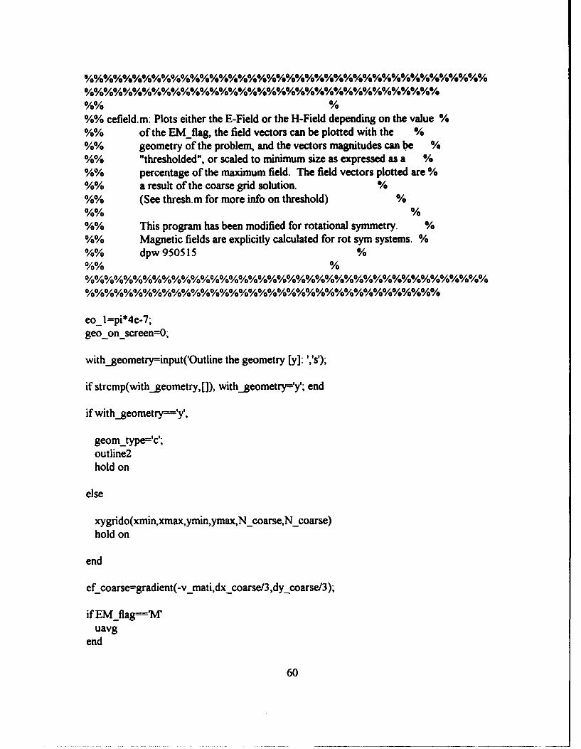
%%%%%%%%%%%%%%%%%%%%%%%%%%%%%%%%%%%%%%%%%% %%%%%%%%%%%%%%%%%%%%%%%%%%%%%%%%%%%%% %% % %% cefield.m: Plots either theE-Field or the H-Field depending on the value % %% of the EM_flag, the field vectors can be plotted with the % %% geometry of the problem, and the vectors magnitudes can Qe % %% "thresholded", or scaled to minimum size as expressed as a % %% percentage of the maximum field. The field vectors plotted are% %% a result of the coarse grid solution. % %% (See thresh.m for more info on threshold) % %% % %% This program has been modified for rotational symmetry. % %% Magnetic fields are explicitly calculated for rot sym systems. % %% dpw 950515 % %% % %%%%%%%%%%%%%%%%%%%%%%%%%%%%%%%%%%%%%%%%%% %%%%%%%%%%%%%%%%%%%%%%%%%%%%%%%%%%%%%
eo _1 =pi•4e-7~ geo _on_ screen=O~
with _geometry=input('Outline the geometry [y]: ','s')~
if strcmp( with _geometry,[]), with _geometry='y'~ end
if with _geometry=='y',
geom_type='c'~
outline2 hold on
else
xygrido( xmin,xmax,ymin,ymax,N _ coarse,N _coarse) hold on
end
ef_ coarse=gradient( -v _ mati,dx _ coarse/3,dy _ coarse/3)~
if EM_ flag=='M' uavg
end
60

if ( cyl_ flag 'C')&(EM _ ftag=='M') rmat _rowc=O:(length(v _ mati)-1 ); rmat_row-rmat_rowc•dx_coarse•(l/3); rmatc=rmat_rowc; numrows=l; while numrows<length(v _ mati)
rmatc=[ rmatc;rmat _rowe]; numrows=numrows+ 1;
end h_tennc=gradient((v_mati.•rmatc),dx_coarse/3,dy_coarsel3); h _ tennc( :,2:length(h _ tennc ))=h _ tennc( :,2:length(h _ tennc) )./ ...
(rmatc( :,2:length(h _ tennc ))); h _ tennc( 1 : length(h_ tennc ),1 )=h _ tennc( 1 :length(h _ tennc ),2) ...
*(1+(4/l)*dx_coarse/3);
j=sqrt( -1 ); hf _coarse=( -1 )*imag( ef _coarse)+( lj)*real(h _ tennc ); hf_coarse=hf_coarse./(eo_1*u_avg_matrix); clear nnatc
end
with_thresh=input('Set threshold for the vectors [n]: ','s');
if strcmp( with_ thresh,[]), with_ thresh='n'; end
if with_ thresh='y',
hold on
if EM _flag 'M',
if cyl_flag 'C' [ xx,yy ]=thresh(( -1 )*imag( ef_ coarse) ./( u _ avg_ matrix*eo _1 ), ...
real(h_tennc) ./(u_avg_matrix•eo_1)); else [yy,xx]=thresh(real(ef_coarse) ./u_avg_matrix •eo_1, ...
imag( ef_ coarse) ./u _ avg_ matrix •eo _1 );
end else
[ xx,yy ]=thresh( real( ef _coarse), -imag( ef_ coarse));
61

end
myquiver(~yy.xmax,ymax, 'r-');
else
ifEM_flag M',
if cyl_ flag 'C' myquiver( ( -1 )*imag( ef _coarse) ./(u _ avg_ matrix*eo _I), ...
real(h_tennc) ./(u_avg_matrix*eo_l),xmax,ymax,'r-');
else myquiver( imag(ef_coarse) ./u_avg_matrix •eo_l, ...
real(ef_coarse) ./u_avg_matrix •eo_l,xmax,ymax,'r-'); end
else
myquiver(real( ef _coarse), -imag( ef _coarse ),xmax,ymax,'r-');
end
end
hold off
o/o %%%%% o/oo/oo/oo/oo/oo/o%o/oo/oo/oo/oo/oo/oo/oo/oo/o%%%%% end of cefield. m o/oo/oo/oo/oo/oo/o%o/oo/oo/oo/oo/oo/o%o/oo/oo/oo/oo/oo/oo/o%o/oo/o%o/oo/oo/oo/oo/oo/o%%%
62

%%%%%%%%%%%%%%%%%%%%%%%%%%%%%%%%%%%%%%%%%% %o/oo/oo/o%%%o/oo/o%%%%%%%%%%o/o%%o/oo/o%%o/o%%%%%o/o%%o/o% %% % %% fefield.m: Plots either the E-Fie:J or the H-Field depending on the value o/o %% of the EM_flag, the field vectors can be plotted with the o/o %% geometry of the problem, and the vectors magnitudes can be % %% "thresholded" or scaled to minimum size as expressed by a % %% percentage of the maximum field. The field vectors plotted are o/o %% a result of the fine grid solution. See thresh.m for more info % %% o/o %% This file has been modified to explicitly cal.:ulate H-field % %% for rotationally symmetric magnetostatic systems. o/o %% dpw 940515 o/o %% %% %% %
% %
%%%%%%%%%%%%%%%%%%%%%%%%%%%%%%%%%%%%%%%%%% %%%%%%%%%%%%%%%%%%%%%%%%%%%%%%%%%%%%%
eo_l=pi*4e-7; geo _on_ screen=O;
with_geometry=input('Outline the geometry [y]: ','s');
if strcmp( with _geometry,[]), with _geometry='y'; end
if with_geometry=='y',
geom _ type='r; outline2 hold on
else
xygrido(xmin,xmax,ymin,ymax,N _fine,N _fine) hold on
end
ef_fine=gradient(-v_source_mat,dx,dy);% (-dV/dx)+j(-dV/dy) z-invar o/c (-dV/dr)+j(-dV/dz) rot sym
63

if EM_ flag 'M' uavg
end
if ( cyl_flag 'C')&(EM _flag='M')
rmat _row=O:(length(v _source_ mat )-1 )~ nnat_row=(nnat_row)*dx~ % dx=dr rmat=rmat_row; numrows=l~
while numrows<length(v _source_ mat) rmat=[ rmat~nnat_row ]~ numrows=numrows+ 1 ~
end h _ term=gradient(( v _source_ mat. *rmat),dx,dy )~
% h_term=(d(rA)/dr)+j(d(rA)/dz)
h_term(:,2:length(h_term))=h_term(:,2Jength(h_term))./ ... (rmat( :,2:length(h _term)))~
% h_term=(l/r)*[(d(rA)Idr)+j(d(rA)/dz)]
h_term(1:length(h_term),1)=h_term(1:length(h_term),2)*(1+(4/3)*dx)~
%2.333 (1+4/3) tennis from coefficient % for values dx from axis % This approach avoids division by zero with accurate results.
j=sqrt(-1 )~ hf_fine=(-1)*imag(ef_fine)+(lj)*real(h_term)~% mag flux density
% -1 is due to the fact that % MATLAB is taking gradient in -z direction
hf_fine=hf_fine./(eo_1*u_avg_matrix)~% hf_fine is now magnetic field matrix dear rmat
end with_thresh=input('Set threshold for the vectors [n]: ','s');
if strcmp( with_ thresh,[]), with _thresh='n'; end
if with_ thresh='y',
hold on
ifEM_flag='M',
64

else
if cyl_ flag 'C [xx,yy]=thresh((-l)*imag(ef_fine) ./u_avg_matrix, ...
real(h _term) ./u _ avg_ matrix)~
else [yy,xx]=thresh(real(ef_fine) ./u_avg_matrix, ...
imag( ef_ fine) ./u _ avg_ matrix); end
else
[ xx,yy ]=thresh( real( ef_ fine), -imag( ef _fine))~
end
myquiver(xx,yy,xmax,ymax,'r-')~
if EM_ flag='M',
if cyl_ flag 'C' myquiver( (-l)*imag(ef_fine) ./u_avg_matrix, ...
real(h_ term) ./u _ avg_ matrix,xmax,ymax, 'r-')~
else myquiver( imag(ef_fine) ./u_avg_matrix, ...
real( ef _fine) ./u _ avg_ matrix,xmax,ymax, 'r-')~ end
else
myquiver(real(ef_fine),-imag(ef_fine),xmax,ymax,'r-')~
end end
hold off
%%%%%%%%%%%%%%%%%%%%%%%%%%%end offefield.m %%%%%%%%%%%%%%%%%%%%%%%%%%%%%%%%%%
65

%%%%%%%%%%%%%%%%%%%%%%%%%%%%%%%%%%%%%%%%%% %%%%%%%%%%%%%%%%%%%%%%%%%%%%%%%%%%%%% %% % %% i_calc.m: Function to perform a closed line integral of the H-Field along % %% the rectangular contour shown below. % %% % %%USAGE: [I]=i_calc(Az,nu,dx,dy) where: Az is the Magnetic vector potential% %% nu is 1/relative permeability % %% o<---(x1,y1)-------------o dx and dy are the grid spacing % %% LLI_LLLIJJJJJJJ % %% I_I_I_I_Current_l_lj_l_lj Az: (MxN) matrix Units: Wb/m% %% l_ljj_ enclosedl_ljj_l_l nu: (M-1 )x(N-1) matrix Units: none % %% 11111111111111 dx and dy: scalar Units: m % %% o--------------(x2,y2)--->o 1: scalar Units: Aim % %% % %%When the function is called, the user will use the crosshairs to indicate % %%the positions of two opposite comers. The function will return the % %% amount of current enclosed or 'error' if the user has entered the comers % %%outside of the region where Az exists or the closed contour contains no % %%area. (i.e. the two comers are do not specify a box) % %% % %% This file has been modified for rot sym systems. dpw 950515 % %% % %%%%%%%%%%%%%%%%%%%%%%%%%%%%%%%%%%%%%%%%%% %%%%%%%%%%%%%%%%%%%%%%%%%%%%%%%%%%%%%
function [i]=i_calc(A,n,dx,dy)~ load mouse.emg -mat~
global cyl_flag
disp(") disp('l. Press the left button for one comer of the box') disp('2. Press the left button again for the other comer') disp('3. Press the right button when you are done') disp(") disp('lf you press the right button immediately after choosing this option') disp('it will take you back to the previous screen.') disp(")
%···················· disp('Press any key to continue ... ') pause
%···················· 66

%plot; [ xx,yy ,button ]=ginput( 1 );
Lower=O; blflag=O; b2flag=O;
while button-=Right_Button I blflag=O I b2flag=O,
ifbutton-Left_Button & Lower=O, blflag=l; x(l)=xx; y(l)=yy; Lower= I;
elseifbutton Left_ Button & Lowe• 1, b2flag=l; x(2)=xx; y(2)=yy; Lower=O;
end
[ xx,yy,button ]=ginput( 1 );
end
x=round(x/dx); y=round(y/dy); [ r,c ]=size( A);
ifsum(x<O) 0 & sum(y<O) 0 & abs(x(l)-x(2))>1 & abs(y(l)-y(2))>1 & ... sum(x>c)==O & sum(y>r)==O,
i=O; uo=pi*4e-7;
ifx(l)>x(2), x=[x(2) x(l)]; end ify(l)<y(2), y=[y(2) y(l)]; end
toprow = r-y(I); bottomrow = r-y(2)-I; leftcol = x( I)+ 1; right col = x(2);
for col=leftcol+ 1 :rightcol
67

nlr_top = O.S*(n(toprow,col-1) + n(toprow,col)); nlr_bottom = 0.5*(n(bottomrow,col-1) + n(bottomrow,col));
i = i + nlr_top • (A(toprow+1,col) - A(toprow,col)) + ... nlr_bottom • (A(bottomrow,col)- A(bottomrow+1,col));
end
for row=toprow+ 1 :bottomrow
ntb_left = 0.5*(n(row-1,1eftcol) + n(row,leftcol)); ntb_right = O.S*(n(row-1,rightcol) + n(row,rightcol));
if cyl_ flag 'C' i = i + ntb_left • (1/(leftcol-0.5)) • ...
((leftcol)* A(row,leftcol+ 1 )-(leftcol-1 )* A(row,leftcol)) ... + ntb_right • (1/(rightcol-0.5)) • ...
((rightcol-1 )* A(row,rightcol)-(rightcol)* A(row,rightcol+ I));
else i = i + ntb _left • (A(row,leftcol+ 1) - A(row,leftcol)) + ...
ntb_right • (A(row,rightcol) - A(row,rightcol+1)); end
end
i=i/uo; x(l )=(x( 1 )+0 .S )*dx; x(2)=(x(2)-0.5)*dx; y(l)=(y(l)-O.S)*dy; y(2)=(y(2)+0.5)*dy; hold on plot([x(l) x(2) x(2) x(1) x(l)],[y(l) y(l) y(2) y(2) y(l)],'cl-') hold off
else
i='error';
end
%%%%%%%%%%%%%%%%%%%%%%end ofi_calc.m %%%%%%%%%%%%%%%%%%%%%%%%%%%%%%%%%Yo%%%%%%
6~

%%%%%%%%%%%%%%%%%%%o/oo/oo/oo/oo/oo/oo/oo/oo/o%%%o/oo/o%o/oo/oo/o%%o/o%% %%%%%%%%%%%%%%%%%%%%%%%%%%%%%%%%%%%%% %% % %% itersoln.m: Used to solve Poisson's equation forE-Statics and M-Statics % %% The equations are formulated using standard Finite Differences% %% and the solution algorithm is a essentially Jacobi's Method % %% with or without a approximate starting solution. o/o %% % %% This program has been modified from its original version % o/o% to solve both z-invariant and rotationally symmetric systems % %% %% Modified 940514 dpw %% % %%%%%%%%o/t%%%%%%%%%%%%%%%%%%%%%%%%%%%%%%%%% %%%%%%%%%%%%%%%%%%%%%%%%%%%%%%%%%%%%% cc=[]~ if EM _flag='M',
prefix=' .im'~ hold_ er=er _matrix~ er _matrix= I ./er _matrix; eo _ _I =pi*4e-7~
else prefix='.ie'~
eo _1 = 118.854e-12~ end
float_ nodes=[]~ num _fnodes=O~ nodes_ around _pee=[]; er _around _pee=[]~ num_nodes=O~ col_index=O; obj_index=O~ charge_ obj=[]; disp(' ') disp('Input the %-error you wish to stop at and specify the maximum number') disp('of iterations.') disp('When either of these two criteria is satisfied, the program stops') disp(' ') TOL=input('lnput the error toi~rance (in percent) [1]: '); if strcmp(TOL,[]). TOL= 1; end TOL=TOUIOO~
disp(' ')
69

MAXITER=input('lnput the maximum number ofiterations [ 1000]: ')~ if strcmp(MAXITER,[]). MAXITER== 1 000~ end MAXITER==round(MAXITER/1 00)*1 00~
%%%%%%%%%%%%%%%%%%%%%%%%%%%%%%%%%%%%%%%%%% %%%%%%%%%%%%%%%%%%%%%%%%%%%%%%%%%%%%% % First, i need to know where all the nodes around all the floating PECIPMR % % objects are . . . % o/~~%%%%%%%%%%%%%%%%%%%%%%%%%%%%%%%%%%%%%%%% %%%%%%%%%%%%%%%%%%%%%%%%%%%%%%%%%%%%%
v _source_ mat==9999*ones(ycells+ 1,xcells+ 1 )~
N==N fine· - . ltable==looktab(N)~
disp(' ') disp('Setting up iterative solver variables . .')
pntr==find(ltable-=0)~
v _source_ mat(pntr )==v _ source(ltable(pntr) );
v _source_ mat==reshape(v _source_ mat,ycells+ 1 ,xcells+ 1 );
for i==1 :max(max(v_source_mat))-10003
fprintft'\nProcessing object #0/c,g- nodes: ',i)
pts _ obj_i=find( v _source_ mat= 1 0003+i)~
[row_ size, col_ size ]==size(pts _ obj_i)~
ifrow_size-=0 & col_size-=0,
obj_index=obj_index+ 1;
col_index=col _index+ I;
float_ nodes( 1 :row_ size,col_index)=pts _ obj_i; num-modes( col_index)=row-size;
row_ index= 1;
70

num _nodes( obj_index)=O~
for j=l :row_size
fprintft'%g 'j)
c _ row=rem(pts _ obj_i(j),ycells+ 1 )~ c _ col=ceil(pts _ obj_i(j)l(xceJJs+ 1 ))~ t_row==c_row-I~ t_col=c_col~
b row==c row+ I~ b col=c col~ - - - -I row==c row~ 1 col=c col-I~ - - - -r row=c row; r col=c col+ I~ - - - -
% look up to see if there is no PEC/PMR
if v _source _mat( t _row ,t _ co1)=9999,
nodes _around _pee( row _index,col_index)=(t_ col-I )*(ycells+ I )+t_row; er _around _pee( row _index, col _index)=( er _matrix( c _row-1 ,c _col-I)+ ...
er_matrix(c_row-I,c_col))/2; num _nodes( obj_index)=num _nodes( obj_index)+ I~ row index=row index+ I~ - -
end
% look left to see ifthere is no PEC/PMR
if v _source_ mat(l_row,l_ col)=9999,
nodes _around _pee( row _index,col_index)=(l_ col-I )*(ycells+ I )+l_row~ er _around _pee( row _index,col_index)=( er _matrix( c _ row-I ,c _col-I)+ ...
er _matrix(c_row,c _col-I ))/2~ num _nodes( obj_index)=num _nodes( obj_ index)+ 1; row index=row index+ I; - -
end
% look right to see if there is no PEC/PMR ifv _source_ mat(r _row,r _ col)=9999,
nodes _around _pee( row _index,col_index)=(r _col-I )*(ycells+ 1 )+r _row; er_around_pec(row_index,col_index)=(er_matrix(c_row-1,c_col)+ ...
er _matrix( c _row,c _ col))/2; num _nodes( obj_index)=num _nodes( obj_index)+ 1;
71

end
row _index=row _index+ 1; end
o/o look down to see if there is no PECIPMR
ifv_source_mat(b_row,b_col)=9999,
nodes_around_pec(row_index,col_index)=(b_col-l)*(ycells+l)+b_row; er _around _pee( row _index,col_index)=( er _matrix( c _row .c _coi-l)+ ...
er _matrix( c _row,c _ col))/2; num _nodes( obj_index)=num _nodes( obj_index)+ 1; row _index=row _index+ 1;
end
fprintft'\n')
end
end
o/o calculate the total charge/current for each PECIPMR object
for i=l :obj_index charge_obj(i)=sum(charge_mat(float_nodes(l :num_fnodes(i),i))); charge_ mat(float _nodes( 1 :num _fnodes(i),i) )=zeros( l,num _ fnodes(i) ); disp(' ') disp(['Charge for object #',int2str(i),': ',num2str(charge_obj(i)),' C/m']) disp(' ')
end
charge_ obj=charge _ obj •eo _1; o/o%o/oo/oo/oo/oo/oo/oo/oo/oo/oo/o%o/oo/oo/oo/oo/oo/o%o/oo/oo/oo/oo/oo/oo/o%%%%%%%%%%%%%%% %%%%%%%%%%%%%%%%%%%%%%%%%%%%%%%%%%%%% o/o Set up pointers to the middle and outer layers % %%%%%%%%%o/o%%%%%o/o%%%%%%%%%o/o%%o/o%%%%%%%%%%%%% %%%%%%%%%%%%%%%%%%%%%%%%%%%%%%%%%%%%%
if cyl_ flag 'C' if EM_ flag 'M'
load cymag_ 51. tgt -mat % coefficients for mag rot sym else
72

load cy803 _51. tgt -mat % coefficients for elect rot sym end
else load in803 _51. tgt -mat % coefficients for z-invariance
end N=N fine+I· - , xmat=table _ 2(N)~
%clear middle _pts outer _pts
disp(") disp('lnitializing pointers to the outer and middle layers')
if exist('outNSl.dat')-=2, for i=1 :2*(xcells+ycells)
outer _pts(i)=find(xmat=i); end save outNSl.dat outer_pts
else load outNSl.dat -mat
end if exist('midNSI.dat')-=2,
for i=2*(xceJJs+yceJJs)+ J :2*(xceJJs+yceJJs)+2*(xcells-2+ycells-2) middle_pts(i-120)=find(xmat=i)~
end save midSt. dat middle _pts
else load midNSl.dat -mat
end
disp(") disp('Set source pointers and media pointers')
source _pts=find(v _source_ mat@9999);
v _lrnown=v _source_ mat( source _pts );
diel_pts=find( v _source_ mat>=9999); [ drow,dcol]=size( diel_pts); v _source_ mat( diel_pts )=zeros( 1 ,drow);
try_ again='y'; load_ success=O;
73

suftix='x'; ig_loaded='n';
o/o to load or not load an initial solution
init_guess=input('Do you wish to use an initial guess? (y]: ','s'); ifstrcmp(init_guess,[]), init_guess='y'; end
if init _guess='y',
if exist('v _mat') 1, disp(' ') ig_loaded=input('Use current coarse grid solution? [y]: ','s'); if strcmp(ig_loaded,[]), ig_loaded=Y; end
end
if ig_loaded='y',
v _source _mat=linterp( v _mat);
else
while try_ again 'y', disp(' ') disp(' Enter the file which contains the initial guess: ') fuame=input('with no file extension: ','s')~ while suffix-='c' & suffix-='£',
disp(' ') disp('Is the data from a coarse or fine grid solution? ')
suffix=input('Enter c or f: ','s'); end
if exist([fiwne,prefix,suffix]) 2, eval(('load ',fname,prefix,suftix,' -mat'])~ try_ again='n'~ load_ success= 1;
else disp(' ')
disp([bell,fuame,prefix,suffix, ... ' does not exist in the current directory!'])
suftix='x'; try_again=input('Do you wish to try again? [y]: ','s')~ ifstrcmp(try_again,[]), try_again=Y~ end
74

end
end
ifload_success=1 & suffix='c', v _source_ mat=linterp( v _mat);
elseif load success 0, disp(' ')
disp([beii,'An initial guess of all zeros will be used', ... '(except known potentials)!']);
v _source_ mat=zeros(N _fine+ 1 ,N _fine+ 1 ); v _source_ mat( source _pts)=v _known;
end
end
else disp(' ') disp([beli,'An initial guess of zeros will be used', ...
'(except known potentials)!']) v _source_ mat=zeros(N _fine+ 1 ,N _fine+ 1 ); v _source _mat( source _pts)=v _known;
end
mesh (flipud(v_source_mat))
disp(") disp('Averaging media properties')
r=(2:ycells)'; c=(2:xcells)';
rt=r-1; rb=r+1; cl=c-1; cr=c+l;
if cyl_ flag 'C' % rotational symmetry cols= 1 :length( c);
75

for k=1 :length(r) cc=(cc;cols];
end ifEM_flag='M'
erl(r,c)=(er _matrix(r-1 ,c-1 )+er _matrix(r,c-1 )). *(l-(2*cc-1 ). "( -1 )); err(r,c)=(er _matrix(r-1 ,c)+er_matrix(r,c)). *(1 +(2*cc+ 1 )."( -1 )); ert(r,c)=er _matrix(r-1,c-1 )+er _matrix(r-1 ,c); erb(r ,c )=er _ matrix(r,c-1 )+er _ matrix(r,c ); erc(r,c)=2*(er_matrix(r-1,c-1) ...
+er _ matrix(r,c-1 )). *( 1 +( 1/2)*(2*cc-1 ). "( -1)) ... +2*(er_matrix(r-1,c) ... +er_matrix(r,c)). *(1-(1/2)*(2*cc+ 1 ). "'( -1 )); %% 2 term is from 1/2 avg of reluctivities
else erl(r,c)=(er _matrix(r-1,c-1 )+er _matrix(r,c-1 )). *(1-(2*cc-1 ). "'( -1 )); err(r,c)=(er _matrix(r-1 ,c)+er _matrix(r,c)). *(I +(2*cc-1 )."( -1 )); ert(r,c)=er _matrix(r-1,c-1 ). *(1-( 4*cc-2). "'( -1)) ...
+er _matrix(r-1 ,c). *(1 +(4*cc-2). "( -1 )); erb(r,c)=er _matrix(r,c-1 ). *(1-( 4*cc-2). "( -1)) ...
+er _matrix(r,c). *(I+( 4*cc-2). "'( -1 )); erc(r,c)=(er_matrix(r-1,c-1 )+er_matrix(r,c-1)). *(2-3*(4*cc-2). "'(-1)) ...
+(er_matrix(r-1,c)+er_matrix(r,c)).*(2+3*(4*cc-2)."(-1)); end
else % z-invariance erl(r,c)=er _matrix(r-1 ,c-1 )+er _matrix(r,c-1 ); err( r,c )=er _matrix( r-1 ,c )+er _matrix( r,c ); ert(r,c)=er_matrix(r-1 ,c-1 )+er _matrix(r-1 ,c); erb(r,c)=er _matrix(r,c-1 )+er _ matrix(r,c); erc(r,c)=2*(erl(r,c)+err(r,c));% 2 term is from 112 of average of epsilons
end den=err(r,c) .I erc(r,c); derl=erl(r,c) .I erc(r,c)~ dert=ert(r,c) .I erc(r,c); derb=erb(r,c) .I erc(r,c);
%from left, right, bottom and top terms!!!
dcharge:_mat=2*eo_1*charge_mat(r,c) .I erc(r,c);
outer _pts=outer _pts'; middle _pts=middle _pts';
76

%%%%%%%%%%%%%%%%%%%%%%%%%%%%%%%%%%%%%%%%%% %%%%%%%%%~~%%%%%%%%%%%%%%%%%%%%%%%%%%%
% The main loop of the iterative algorithm % %%%%%%%%%%%%%%%%%%%%%%%%%%%%%%%%%%%%%%%%%% %%%%%%%%%%%%%%%%%%%%%%%%%%%%%%%%%%%%% disp(' ') disp('Starting the iterative solver now ... HEAVY NUMBER CRUNCHING')
N=lOO~
error=O; direction=+ 1; % error is going up instead of down. done='n'~
iterations=O; errordat=f1·
L- •
sinfdat=[}~
while done=='il',
while iterations < MAXITER & (error > TOL I (error <= TOL & direction= 1) ),
%for 96 iterations do not calculate the norm s(n), becuase it is an % expensive operation, do this for the last four iterations of every % 1 00 iterations
for q=1:96
% apply Poission's equation to every point
v_source_mat(r,c)=dcharge_mat + v_source_mat(r,cr).*derr + ... v _source _mat(r,cl). *derl+v _source_ mat(rb,c )_ *derb+ . _. v _source_ mat( rt, c). • dert~
% reset the source points back to their known values
v _source_ mat( source _pts )=v _known;
% for each floating PEC/PMR object enforce the appropriate boundary %conditions, flux ofD equals zero and equipotential (forE-statics) %or H normal equals zero, equipotential, and curl ofH equals zero %(forM-statics)
for j=l :obj_index
n _ num=num _ nodes(j);
77

f _ num=num _ fnodes(j)~ e_a_p==er_around_pec(I :n_numj)~
v_source_mat(float_nodes(I :f_numj))=ones(l,f_num)*(charge_objG) + ... v _source_ mat( nodes_ around _pee( I :n _ numj))'* e _a _p )/ sum( e _a _p );
end
%fix the boundary nodes with the TGT matrix to simulate the "open" %boundary
v _source _mat( outer _pts )=inside*v _source_ mat( middle _pts )~
end
% for the last four iterations of every 100, calcualate s(n)
for q=l:4
end
v_source_mat(r,c)=dcharge_mat + v_source_mat(r,cr). *derr + ... v _source_mat(r,cl).*derl+v _source_mat(rb,c). *derb+ ... v _source_mat{rt,c). *dert~
v _source_ mat( source _pts )=v _known;
for j=l :obj_index
n _ num=num _ nodes(j)~ f_ num=num _ fnodes(j); e _ a_p=er _around _pee( 1 :n _ numj)~
v _source_ mat(float_nodes( 1 :f_ numj))=ones( l ,f_ num)*( charge_ obj(j) + ... v_source_mat(nodes_around_pec(l :n_numj))'* e_a_p)/ sum(e_a_p);
end
v _source_ mat( outer _pts )=inside*v _source_ mat( middle _pts )~
s(q)=sum(sum(v_source_mat ."2));
78

%using the last three norms (s(n)), calculate the lambda coefficient and % the estimated norm as iterations->infinity to give a more accurate % determination of the actual error
lambda 1 =(s(3)-s(2))/( s(2)-s(1 ))~ s_infinity1 =(s(3)-lambda1*s(2))1( 1-lambda1 );
lambda2=(s( 4)-5(3 ))/(s(3 )-s(2)); s_infinity2=(s(4)-lambda2*s(3))/(1-lambda2);
s _infinity=( s _infinity 1 +s _infinity2 )12~
olderror=error~
error=abs((s( 4)-s_infinity)/s( 4));
errordat=[errordat error]~ sinfdat=[ sinfdat s _infinity];
direction=sign( error-olderror );
iterations=iterations+ 1 00; disp(' ') disp(['Estimated Error: ',num2str( error*1 00), ...
'Iterations: ',int2str(iterations), ... 'S_inf: ',num2str(s_infinity)])
end
mesh(flipud( v _source_ mat))
done='y'~
if error@=TOL, disp(' ') disp([bell, 'The specified error (',num2str(TOL *100), ...
'%)has been reached.']) disp(' ') disp(['The current number of iterations: ',int2str(iterations)])
end
if iterations>=MAXITER,
79

disp(' ') disp([bell, 'The maximum number of iterations has been reached, ', ...
int2str(MAXITER),' iterations.']) disp(' ') disp(['The current estimated error is: ',num2str( error• I 00), '%.'])~
end
disp('') newerror=input('Do you wish to modify this? [n] ','s')~ if strcmp(newerror,[]), newerror='n'~ end if newerroa 'y',
done='n'~
while (error<=TOL I iterations>=MAXITER) & done 'n',
done='n'~ disp('')
TOL=input('New error tolerance(%): ')/100~ MAXITER=input('New maximum# ofiterations (UNITS OF 100!): ')•too~
if error<=TOL I iterations>=MAXITER, disp('')
disp([bell, 'One or both of those conditions is already ', ... 'satisfied! '])
disp('') done=input('Do you wish to try again? [y]','s')~
if done-'n', done='y'~
else done='n'~
end
else
disp('') disp('Continuing iterative solver ... ')
end
80

end
end
end
if EM _flag 'M', er _matrix= hold_ er~ eo _1 =l/8.854e-12~
end
clear dcharge _mat derr dert derb derl f_ num n _ num e _ a_p
%%%%%%%%%%%%%%%%%%%%%%%%end ofitersoln.m %%%%%%%%%%%%%%%%%%%%%%%%%%%%%%%%%%%
81

%%%%%%%%%%%%%%%%%%%%%%%%%%%%%%%%%%%%%%%%%% %%%%%%%%%%%%%%%%%%%%%%%%%%%%%%%%%%%%% %% % %% makesys2.m: This program will generate the system matrix for the coarse % %% grid using the geometry media and the TGT coefficients. This % %% system matrix sys _mat will then be modified by matsolve.m % %% using the appropriate source and object boundary conditions. % %% % %% This program has been modified to generate the coarse grid % %% system matrix for both z-invariant and rotationally symmetric % %% systems. dpw 940514 % %% % %% Note that different code is required for rotationally % %% symmetric electrostatic and magnetostatic problems. % %%%%%%%%%%%%%%%%%%%%%%%%%%%%%%%%%%%%%%%%%% %%%%%%%%%%%%%%%%%%%%%%%%%%%%%%%%%%%%%
ifEM_flag='M', %forM-statics the er matrix hold_er=er_matrix_coarse; %hold the value of relative er_matrix_coarse=l .I er_matrix_coarse; %permeability. eo_l=pi*4E-7;
end
if cyl_flag='C' % rotationally symmetric system
ifEM_flag='M' load cymag_l7.tgt -mat % tgt matrix for magnetostatics (rot sym)
else load cy267_17.tgt -mat % tgt mat for electrostatics (rot sym)
end
else % z-invariant system load in267 _17.tgt -mat
end
N=N _coarse; % # of cells for coarse grid ltable=looktab(N); % call lookup table routine
%%%%%%%%%%%%%%%%%%%%%%%%%%%%%%%%%%%%%%%%%% %%%%%%%%%%%%%%%%%%%%%%%%%%%%%%%%%%%%% %Now, make the matrix!!!! % %%%%%%%%%%%%%%%%%%%%%%%%%%%%%%%%%%%%%%%%%% %%%%%%%%%%%%%%%%%%%%%%%%%%%%%%%%%%%%%
82

sys_mat=zeros((N+l)*(N+l)-4,(N+l)*(N+l)-4); % "-4" is to exclude the four rhs=zeros((N+1)*(N+1)-4,1); %comers in the system matrix
for eq_num=4*N-3:(N+l)*(N+1)-4 %equation# starts at 4N-3 becuase the first % 4N-4 equations come from the TGT boundary % condition matrix
pntr=find(ltable==eq_num); %point to the grid point for equation#: eq_num
c _row=rem(pntr,N+ 1 ); c _ col=ceil(pntr/(N+ 1 ));
% current row and column of geometry converted % from the "find" commmand's indexing scheme
t_row=c_row-1;, t_col=c_col; %top row and column b_row=c_row+I;, b_col=c_col; %bottom row and column l_row=c _row;, 1_ col=c _col-I; % left row and column r _row=c _row;, r _ col=c _col+ 1; % right row and column
t_num=(t_col-l)*(N+l)+t_row; %convert row and column info ofthe above b _ num=(b _col-I )*(N+ I )+b _row; % variables back into the "find" -indexing l_num=(l_col-l)*(N+l)-~l_row; %scheme r _ num=( r _col-I )*(N+ 1 )+r _row;
% pre-calculate the averaging of the media
%% Rotationally Symmetric Systems if cyl_ flag 'C' % rotationally symmetric systems if EM_ flag='M'
er_top = er_matrix_coarse(c_row-l,c_col-1) ... +er _matrix_ coarse( c _row-1 ,c _col);
er_bottom =er_matrix_coarse(c_row,c_col-1) ... +er _matrix_ coarse( c _row,c _col);
er_left =( er _matrix_ coarse( c_row-l,c_ col-I) ... +er_matrix_coarse(c_row,c_col-1)) ... *(l-11(2*(c_col-l)-I));
er _right =( er _matrix_ coarse( c _row-1 ,c _col) ... +er_matrix_coarse(c_row,c_col)) ... *( 1 + 11(2*( c _col-I)+ 1 ));
er _center =( er _matrix_ coarse( c _row- I ,c _col) ... +er_matrix_coarse(c_row,c_col)) ... *(l-(l/2)*(11(2*(c_col-l)+ 1))) ... +( er _matrix_ coarse( c _row-1 ,c _coi-l) ... +er_matrix_coarse(c_row,c_col-1)) ... *(1 +(l/2)*(11(2*(c_ coi-l )-1 )));
83

else a_ col=c _col-I; % actual column away from centerline er_top =er_matrix_coarse(c_row-I,c_col-1)*(1-I/(4*a_col-2)) ...
+er _matrix_ coarse( c _row-I,c _col )*(I+ I/( 4*a_ col-2)); er _ bottom=er _matrix_ coarse( c _row,c _col-I)*( 1-II( 4 •a_ col-2)) ...
+er _matrix_ coarse( c _row,c _col )*(1 + 1/( 4*a _ col-2)); er _left =( er _matrix_ coarse( c _row-I,c _col-I) ...
+er _matrix_ coarse( c _row,c _col-I))*( 1-1/(2*a_ col-1 )); er_right =(er_matrix_coarse(c_row-l,c_col) ...
+er_matrix_coarse(c_row,c_col))*(l+l/(2*a_col-l)); er _center=( er _matrix_ coarse( c _row-I,c _col-I) ...
+er_matrix_coarse(c_row,c_col-l))*(l-3/(8*a_col-4)) ... +( er _matrix_ coarse( c _row-l,c _col) ... +er_matrix_coarse(c_row,c_coi))*(I+3/(8*a_col-4));
end
else %% z-invariant systems er _top =er _matrix_ coarse( c _row-l,c _col-I )+er _matrix_ coarse( c _row-l,c _col); er_bottom=er_matrix_coarse(c_row,c_col-1) +er_matrix_coarse(c_row,c_col); er _left =er _matrix_ coarse( c _row-I.e_ col-I )+er _matrix_ coarse( c _row,c _coi-l); er _right =er _matrix_ coarse( c _row-1 ,c _col) +er _matrix_ coarse( c _row ,c _col); er _ center=er _ top+er _bottom;
end % fill the system matrix!
sys _mat( eq_num,eq_ num) =-2*er _center; sys_mat(eq_num,Jtable(t_num))=er_top; sys _mat( eq_ num,ltable(b _ num) )=er _bottom; sys _mat( eq_ num,ltable(l_ num) )=er _left; sys _mat( eq_ num,ltable( r _ num) )=er _right;
% generate the Right hand side forcing function
rhs( eq_ num)=-2 *charge_ mat_ coarse( c _row ,c _ col)*eo _I;
end
%%%%%%%%%%%%%%%%%%%%%%%%%%%%%%%%%%%%%%%%%% %%%%%%%%%%%%%%%%%%%%%%%%%%%%%%%%%%%%% % Modify the inside matrix of tgt coefficients to exclude the 4 comers % %%%%%%%%%%%%%%%%%%%%%%%%%%%%%%%%%%%%%%%%%% %%%%%%%%%%%%%%%%%%%%%%%%%%%%%%%%%%%%%
84
--- ----------

insidep=[inside(2 :N,: )~ inside(N+2:2*N,:); inside(2*N+2:3*N,:); inside(3 *N+ 2:4 *N,:) ];
insidepp=[inside( 1,: ); inside(N+ 1,: ); inside(2 *N+ 1,: ); inside(3*N+ 1,:)];
[ r _ inp,c _inp ]=size(insidep );
sys _mat( 1 :r _inp,r _inp+ 1 :r _ inp+c _ inp )=insidep; sys_mat(l :r_inp, 1 :r_inp)=-eye(r_inp);
ifEM_flag 'M', er _matrix_ coarse= hold_ er;
end
%%%%%%%%%%%%%%%%%%%%%%%%%%end ofmakesys2.m %%%%%%%%%%%%%%%%%%%%%%%%%%%%%%%%%%
85

%%%%%%%%%%%%%%%%%%%%%%%%%%%%%%%%%%%%%%%%%% %%%%%%%%%%%%%%%%%%%%%%%%%%%%%%%%%%%%% %% %% This will be used to augment the iterative solver by using %% sparse matrices to solve fine grid system. Updated 9405 14 dpw %% %% makesysfm: This program will generate the system matrix for the fine %% grid using the geometry media and the TGT coefficients. This %% system matrix sys_mat will then be modified by matsolvfm %% using the appropriate source and object boundary conditions. %% This program handles either rotationally symmetric or %% z-invariant systems. %% %% o/oo/oo/oo/oo/oo/oo/oo/oo/oo/oo/oo/oo/oo/oo/oo/oo/oo/oo/oo/oo/oo/oo/oo/oo/oo/oo/oo/oo/oo/oo/oo/oo/oo/o%%%%%%%% %%o/oo/oo/oo/oo/oo/oo/oo/oo/oo/oo/oo/oo/oo/oo/oo/oo/oo/oo/o%o/oo/oo/oo/oo/oo/oo/oo/oo/oo/oo/oo/oo/oo/oo/o
if EM _flag='M', hold_ er=er _matrix~ er _matrix= 1 ./ er _matrix~ eo_l=pi*4E-7;
end
o/o for M-statics the er _matrix o/o hold the value of relative
o/o permeability.
if cyl_ flag 'C' o/o rotationally symmetric system
if EM_ flag 'M' load cymag_ 51. tgt -mat
else load cy803 _51. tgt -mat
end
else o/o z-invariant system load in803_5l.tgt -mat
end
N=N_fine; o/o #of cells for coarse grid ltable=looktab(N)~ o/o call lookup table routine
%o/oo/oo/oo/oo/oo/oo/oo/oo/oo/oo/o%o/oo/oo/oo/oo/oo/oo/oo/oo/oo/oo/oo/oo/oo/oo/oo/oo/oo/oo/o%o/oo/oo/oo/oo/oo/oo/oo/o% o/oo/oo/oo/oo/oo/oo/oo/oo/oo/oo/oo/oo/oo/oo/oo/oo/oo/oo/oo/oo/oo/oo/oo/oo/oo/oo/oo/oo/oo/oo/oo/oo/oo/oo/oo/oo/o %Now, make the matrix!!!! o/o o/oo/oo/oo/oo/oo/oo/oo/oo/oo/oo/oo/oo/oo/oo/oo/o%%%%%o/oo/oo/oo/oo/oo/oo/oo/oo/oo/oo/oo/oo/oo/oo/oo/oo/oo/oo/oo/oo/o o/oo/o%%%%o/oo/oo/oo/oo/o%%o/oo/oo/oo/oo/oo/oo/oo/oo/o%o/oo/oo/oo/oo/oo/oo/oo/oo/oo/oo/oo/oo/oo/o
86
..... ··~---~-------------------------------------'

sys_mat=sparse((N+1)*(N+1)-4,(N+1)*(N+1)-4)~ % "-4" is to exclude the four rhs=sparse((N+ l )*(N+ l )-4, I)~ % corners in the system matrix
for eq_num=4*N-3:(N+l)*(N+I)-4 %equation# starts at 4N-3 becuase the first % 4N-4 equations come from the TGT boundary % condition matrix
pntr=find(ltable eq_num)~ %point to the grid point for equation#: eq_num
c _row=rem(pntr,N+ 1 )~ c _ col=ceil(pntr/(N+ 1) )~
% current row and column of geometry converted % from the "find" commmand's indexing scheme
t_row=c_row-1~. t_col=c_col~ %top row and column b _row=c _row+ 1 ~. b _ col=c _col~ % bottom row and column l_row=c_row~, l_col=c_col-1~% left row and column r _row=c _row~. r _ col=c _col+ 1 ~ % right row and column
t_num=(t_coi-1)*(N+I)+t_row~ %covert row and column info ofthe above b_num=(b_col-l)*(N+l)+b_row~ %variables back into the "find"-indexing l_num=(l_col-1)*(N+1)+l_row~ %scheme r num=(r col-1)*(N+ l)+r row~ - - -
% pre-calculate the averaging of the media
if cyl_ flag='C' % rotationally symmetric system if EM_ flag 'M'
er_top = er_matrix(c_row-l,c_col-1) ... +er _matrix( c _row-1 ,c _col)~
er _bottom =er _matrix( c _row,c _col-I) ... +er _matrix( c _row,c _col)~
er _left =( er _matrix( c _row- I ,c _col-I) ... +er_matrix(c_row,c_col-I)) ... *(1-11(2*(c_col-I)-I))~
er _right =( er _matrix( c _row- I ,c _col) ... +er_matrix(c_row,c_col)) ... *(I+ 11(2 *( c _col-I)+ I));
er_center =(er_matrix(c_row-I,c_col) ... +er_matrix(c_row,c_col)) ... *(I-(l/2)*(11(2*(c_col-I)+ I))) .. . +( er _matrix( c _row- I ,c _col-I) .. . +er_matrix(c_row,c_coi-I)) ... *(I +(112)*(11(2*( c _col-I )-I)));
87
else a_ col=c _col-I ~ % actual column away from centerline er _top =er _ matrix(c_row-1 ,c_ col-I )*(1-l/(4*a_col-2)) ...
+er_matrix(c_row-l,c_col )*(I+ l/(4*a_col-2))~ er _ bottom=er _matrix( c _row,c _col-I)*( 1-1/( 4 •a_ col-2)) ...
+er_matrix(c_row,c_col )*(1+11(4*a_col-2))~ er _left =( er _matrix( c _row- I ,c _col-I) ...
+er _matrix(c_row,c_col-1 ))*(1-11(2*a_ col-I))~ er_right =(er_matrix(c_row-l,c_col) ...
+er _matrix(c_row,c _ col))*(l + l/(2*a_ coi-l))~ er _center=( er _matrix( c _row- I ,c _col-I) ...
+er_matrix(c_row,c_col-I))*(l-3/(8*a_col-4)) ... +(er_matrix(c_row-l,c_col) ... +er_matrix(c_row,c_col))*(l +3/(8*a_col-4))~
end else %% z-invariant system er _top =er _matrix(c_row-1 ,c _col-I )+er _matrix(c_row-1 ,c_ col)~ er _ bottom=er _matrix( c _ row,c _col-I) +er _matrix( c _row,c _col)~ er _left =er _matrix( c _row- I ,c _ col-1 )+er _matrix( c _row,c _col-I)~ er _right =er _matrix( c _row-1 ,c _col) +er _matrix( c _row,c _col); er _ center=er _ top+er _bottom~
end %fill the system matrix!
sys_ mat( eq_ num,eq_num) =-2*er _center; sys_mat(eq_num,ltable(t_num))=er_top~
sys _mat( eq_ num,ltable(b _ num) )=er _bottom; sys _mat( eq_ num,ltable(l_ num) )=er _left; sys _mat( eq_ num,ltable(r _ num) )=er _right;
% generate the Right hand side forcing function
rhs(eq_num)=-2*charge_mat(c_row,c_col)*eo_l~
end
%%%%%%%%%%%%%%%%%%%%%%%%%%%%%%%%%%%%%%%%%% %%%%%%%%%%%%%%%%%%%%%%%%%%%%%%%%%%%%% % ModifY the inside matrix of tgt coefficients to exclude the 4 comers % %%%%%%%%%%%%%%%%%%%%%%%%%%%%%%%%%%%%%%%%%% %%%%%%%%%%%%%%%%%%%%%%%%%%%%%%%%%%%%%
88

insidep=[inside(2:N,:); inside(N+2:2•N,: ); inside(2•N+2:3•N,:); inside(J•N+2:4•N,:)];
insidepp=[inside( 1,: ); inside(N+ 1,: ); inside(2•N+ 1,:); inside(3 •N+ I,:)];
[ r _inp,c _inp ]=size(insidep );
sys _mat( 1 :r _inp,r _inp+ I :r _inp+c _inp )=insidep; sys_mat(1 :r_inp, 1 :r_inp)=-eye(r_inp);
if EM_ flag 'M', er _ matrix=hold _ er;
end
%%%%%%%%%%%%%%%%%%%%%%%%%%end ofmakesysfm %%%%%%%%%%%%%%%%%%%%%%%%%%%%%%%%%%
89

%%%%%%%%%%%%%%%%%%%%%%%%%%%%%%%%%%%%%%%%%% %%%%%%%%%%%%%%%%%%%%%%%%%%%%%%%%%%%%% %% This will be used to augment the iterative solver by %% using sparse matrices to slve the fine grid system. %% Updated 940107 dpw. o/oo/o %% %% matsolvfm: This program will use the sys_mat from makesysfm and the %% source information from voltsrc.m and chargsrc.m and and solve %% the system of equations for the fine grid. %% %%o/o%%%%%o/oo/oo/oo/oo/oo/oo/o%o/o%o/oo/oo/oo/oo/o%%o/oo/oo/oo/o%%%%%%%%%%%%% %%%%%%%%%%%%%%%%%%%%%%%%%%%%%%%%%%%%%
k=(xcells+ 1 )•(ycells+ 1 )-4; v _pntr-1 : k; ep _rem_ col_flag=[]; kp _rem_ col_ flag=[]; keep_ col_ flag=[]; keep _row_ flag=[];
o/o find all the floating PECIPMR. and eliminate the need to solve for them, only o/o need to solve for one of the potentials for each object
for i=1 :num_pec_obj
equal _pots=find( v _source 1 0000+ J+i);
[ dum,num _ eq__pots ]=size( equal _pots);
while num _ eq__pots> 1,
% adding the rows and columns of the equal pots and set the first o/o row and column number (equal_pot(1)) to the sum, also add the charges % on the floating objects
sys _mat( :,equal _pots( 1) )=sum( sys _mat(: ,equal _pots)')'; sys _mat( equal _pots( 1 ), :)=sum( sys _mat( equal _pots,:)); rhs( equal _pots( 1) )=sum( rhs( equal _pots));
% set the equi-potential remove column flag to the rows and column
90

% corresponding to the floating potentials we don't need to solve for %anymore.
ep _rem_ col_ flag=[ ep _rem_ col_ flag equal _pots(2:num_eq_pots)]~
v _pntr( equal _pots(2 :num _ eq_pots) )=equal _pots( 1 )•ones( 1 ,num _ eq_pots-1 );
num _ eq_pots=O;
end
end
% find all the known potentials
vs=zeros(1,k)~
known _pots=find(v _source@9999)~ [ dum,num _ kn _pots ]=size(known _pots)~ vs(known _pots)=v _ source(known _pots)~
kp _rem_ col_ flag=known _pots;
fori=1:k
%if either of the flags below contain "i" then keep that row and column % (i.i. set flag!)
ifsum(ep_rem_col_flag i)==O & sum(kp_rem_col_flag i)==O,
keep_col_flag=[keep_col_flag i]~
keep _row _flag=[keep _row_ flag i]~
end
end
% modified the rhs due to the known potentials
rhs=sparse(-sys_mat•(vs(1 :k)')+full(rhs))~
sys_ mat=sys _ mat(keep _row_ flag,keep _ col_flag)~ % prune the system matrix based rhs=rhs(keep _row_ flag, 1 )~ % on the flags set above
91

---------- -------------~---
%solve the system! EXPLOIT SPARSITY
v=full( sys _ mat\rhs ); v _pntr==v _pntr( 1,keep _row_ flag)'; v _soln(v _pntr)=v; % put back all the equi-potentials for the floating PECIPMR objects for i= 1 :num_pec _ obj
equal _pots=find( v _source 1 0000+ 3+i);
[ dum,num _ eq_pots ]=size( equal _pots);
while num _ eq_pots> 1,
v _ soln( equal _pots )=v _ soln( equal _pots( 1 ))•ones( 1,num _ eq_pots );
num _ eq_pots=O;
end
end v _soln(known _pots)=v _ source(known_pots); % put the solution into a matrix form so that results can be displayed v _source_ mat=zeros(ycells+ 1,xcells+ 1 ); for i=1:k
pntr=find(ltable=i); v _source_ mat(pntr)=v _ soln(ltable(pntr));
end
% fix the comers, since they were not included in the system matrix
v_comer=insidepp•v_soln(xcells•4-3:xcells•4-3+ ... (xcells-2)•4-l )';
v _source_ mat( 1, 1 )=v _comer( 1 ); v _source_ mat( 1 ,xcells+ 1 )=v _ comer(2); v _source_ mat(ycells+ 1 ,xcells+ 1 )=v _ comer(3 ); v _source_ mat(ycells+ 1, 1 )=v _comer( 4);
%%%%%%%%%%%%%%%%%%%%%%%%%end of matsolvf.m %%%%%%%%%%%%%%%%%%%%%%%%%%%%%%%%%%
92

%%%%%%%%%%%%%%%%%%%%%%%%%%%%%%%%%%%%%%%%%% %%%%%%%%%%%%%%%%%%%%%%%%%%%%%%%%%%%%% %% % %% q_calc.m: Function to perfonn a flux integral of the D-Field through the % %% rectangular "surface" shown below. % %% % %%USAGE: [Q]=q_calc(V,er,dx,dy) where: Vis the Electric potential % %% er is relative permittivity % %% o<--(x1,y1)--------------o dx and dy are the grid spacing %
%% IJJJJJJJJJJJJJ % %% IJJJJChargej_IJjJJ V: (MxN) matrix Units: V % %% LLLL enclosediJJJJJ er: (M-1 )x(N-1) matrix Units: none % %% 11111111111111 dx and dy: scalar Units: m % %% o------------(x2,y2)--->o Q: scalar Units: C/m (z-invariant)% %% C (rotational sym)% %% When the function is called, the user will use the crosshairs to indicate % %% the positions of two opposite comers. The function will return the o/o %% amount of charge enclosed or 'error' if the user has entered the comers % %% outside of the region where V exists or the closed surface contains no % %%volume. (i.e. the two comers do not specifY a box) % %% % %% This program has been modified to accomodate rotational symmetry % %% dpw 940430 % %%%%%%%%%%%%%%%%%%%%%%%%%%%%%%%%%%%%%%%%%% %%%%%%%%%%%%%%%%%%%%%%%%%%%%%%%%%%%%%
function [q]=q_calc(v,e,dx,dy)~ load mouse.emg -mat~ global cyl_ flag disp(") disp(' 1. Press the left button for one comer of the box') disp('2. Press the left button again for the other comer') disp('3. Press the right button when you are done') disp(") disp('lf you press the right button immediately after choosing this option') disp('it will take you back to the previous screen.') disp(")
%···················· disp('Press any key to continue ... ')
%···················· pause
[xx,yy,button]=ginput(1)~
93

blflag=O~ b2flag=O~
Lower=O~
while button-=Right_Button I blflag==O I b2flag==O,
ifbutton Left_Button & Lower==O, blflag=l; x(l)=xx; y(l)=yy; Lower= I;
elseifbutton Left_Button & Lowe•-1, b2flag=l; x(2)=xx~
y(2)=yy; Lower=O;
end
[ xx,yy ,button ]=ginput( 1 );
end
x=round(xldx); y=round(y/dy); [r,c]=size(v);
ifsum(x<O)=O & sum(y<O)=O & abs(x(l)-x(2))>1 & abs(y(l)-y(2))>1 & ... sum(x>c)==O & sum(y>r)==O,
q=O; eo=8.854e-12;
ifx(l)>x(2), x=[x(2) x(l)]; end ify(l)<y(2), y=[y(2) y(l)]; end
toprow = r-y(l ); bottomrow = r-y(2)-1; leftcol = x(l)+l~ rightcol = x(2)~
for col=leftcol+ 1 :rightcol
elr_top = o.s•(e(toprow,col-1) + e(toprow,col));
94
------------------~-

elr bottom= O.S*(e(bottomrow,col-1) + e(bottomrow,col)); if cyl_ flag 'C
q = q + (elr_top • (v(toprow+1,col) - v(toprow,col)) + ... elr_bottom • (v(bottomrow,col)- v(bottomrow+1,col))) ... *(2*pi*( col- l/2)*dx);
else q = q + elr_top • (v(toprow+l,col) - v(toprow,col)) + ...
elr_bottom • (v(bottomrow,col)- v(bottomrow+l,col)); end
end for row=toprow+ I :bottomrow
etb_left = 0.5*(e(row-1,1eftcol) + e(row,leftcol)); etb_right = 0.5*(e(row-l,rightcol) + e(row,rightcol));
if cyl_flag 'C' q = q + etb _left • (v(row ,leftcol+ I) - v(row,leftcol)) ...
• (2*pi*(leftcol-I/2)*dy) + ... etb_right • (v(row,rightcol) - v(row,rightcol+1)) ... • (2*pi*(rightcol-ll2)*dy);
else q = q + etb_left • (v(row,leftcol+1)- v(row,leftcol)) + ...
etb _right • (v( row,rightcol) - v(row ,right col+ 1)) end
end
x(l)=(x(1)+0.5)*dx; x(2)=(x(2)-0.5)*dx; y(1)=(y(1)-0.5)*dy; y(2)=(y(2)+0.5)*dy;
hold on plot([x(1) x(2) x(2) x(1) x(1)],[y(l) y(1) y(2) y(2) y(l)],'c1-') hold off
else q='error';
end
%%%%%%%%%%%%%%%%%%%%%%end ofq_calc.m %%%%%%%%%%%%%%%%%%%%%%%%%%%%%%%%%%%%%%%%
95

%%%%%%%%%%%%%%%%%%%%%%%%%%%%%%%%%%%%%%%%%% %%%%%%%%%%%%%%%%%%%%%%%%%%%%%%%%%%%%% %% % %% solndom.m: This is used to start a new EM-Static problem. It is chosen to % %% initialize a new solution domain. % %% updated 940101 dpw % %%%%%%%%%%%%%%%%%%%%%%%%%%%%%%%%%%%%%%%%%% %%%%%%%%%%%%%%%%%%%%%%%%%%%%%%%%%%%%%
clc
newdomain='y'~
if domain_ flag 1,
newdomain=input([bell,'W ARNING: TillS WILL ERASE YOUR PREVIOUS', ... ' DOMAIN, CONTINUE [n]?: '],'s')~
if strcmp(newdomain,[]), newdomain='n'~ end
end
if newdomain='y',
domain_ flag= 1 ~
c1c disp(' DOMAIN REGION SCREEN ') disp('') disp('The dimension entered here determines the area in which you will') disp('place your sources and media geometry. This area is bordered by ') disp('the dashed blue line around the blue grid. ') disp(")
rot_sym=input('Do you want to solve a rotationally symmetric system? [n] ','s')~ ifstrcmp(rot_sym,[]), rot_sym='R'~ end if (rot_sym='y')l(rot_sym='Y')
cyl_ flag='C'~ ifEM_flag 'E'
enclosed str='C'· - , else
enclosed str 'A *m'· - , end
else
96

cyl_flag='R';
end xmax=-9999; xmin=O; while xmax@O,
xrnax=input(['Enter the dimension (in meters) of a', ...
if strcmp( xmax,[]), xmax=-1; end ifxmax@O,
' square solution domain: 1);
disp([beii.'Only positive dimensions in this world, thank you!']); end
end ymin=O; ymax=xmax; xcells=N fine-2; ycells=N _fine-2; dxp=(xmax-xmin)/xcells; dyp=(ymax-ymin)/ycells; ymax=ymax+2*dyp; xmax=xmax+2*dxp; xcells=xcells+2; ycells=ycells+2; er _ matrix=ones(ycells,xcells ); v _source=9999*ones((xcells+ 1 )*(ycells+ 1 ), 1 ); v _source_ coarse=9999*ones((N _coarse+ 1 )*(N _coarse+ 1 ), 1 ); pee _pt _ matrix=zeros(ycells+ 1 ,xcells+ 1 ); pee_ com_ matrix=zeros(2*ycells+ 1 ,2*xcells+ 1 ); pcm=pec _ com_matrix; dx=(xmax-xmin)lxcells; dy=(ymax-ymin)lycells; charge_ mat=zeros(ycells+ I ,xcells+ 1 ); charge_ mat_ coarse=zeros(N _coarse+ 1 ,N _coarse+ 1 ); cg_made=O; geom_ type='f; redraw2
~···················· pause
~··················· hold off
end ~~~~~~~~~~~~~~~~~~~~~~~~~~end ofsolndom.m ~~~~~~~~~~~~~~~~~~~~~~~~~~~~~~%%%~%
97

APPENDIXB MATRIX METHOD TGT PROGRAMS
o/o coefgenc.m o/o This program will generate TGT coefficients using the % matrix solution method for rotationally symmetric electrostatic systems. % Functions required include: makemmc.rn, makemlc.m and makemnc.m. % Author: David P. Wells %Date oflast revision: 940116 M=input('Enter the Far Dirichlet Boundary Dimension')~ N=input('Enter the Computational Grid Dimension ')~ M=M-2~ garnmac=makemmc(M,N); whileM>N+2
M=M-2~ gammac=sparse(makemmc(M,N)-sparse(makemlc(M,N)*inv(gammac) ...
*makemnc(M+2,N))); end TGT=( -1 )*(inv(gammac )*makemnc(M,N)); TGT=[TGT;TGT(3*N+2,:)]; %%Adding left side TGT coefficients TGT=[TGT(l,:);TGT]; %%based on symmetry. TGT(4*N+4,l)=l; for i=3*N-2:4*N-4
TGT(i+ 7 ,i)= 1 ~ end TGT=full(TGT);
98

function [ x ]=makemlc(M.N)~ % This function makes the Ml matrix for generating TGT %coefficients given the desired size ofM (right side oflayer) %and N (computational grid dimension) % for rotationally symmetric systems. %David P. Wells 940302 l=N+2*M+2~ m=l-4; top=N+(M-N)/2; r=top-1/2~ side=M; x=sparse( m,l)~ row=1; col= I; for i=l:top
x(row,col)=-1 ~ row=row+l~
col=col+1; end col=col+1; row=row-1; for i=1:M
x(row,col)=-1*(1+ 1/(2*r)); row=row+1; col=col+1;
end col=col+1; row=row-1~
for i=1:top x(row,col)=-1; row=row+1; col=col+l~
end
99

Ml-full(makemlc(S,3))
Ml= Columns 1 through 6
-1 0 0 0 0 0 0 -1 0 0 0 0 0 0 -1 0 0 0 0 0 0 -1 0 -Bn 0 0 0 0 0 0 0 0 0 0 0 0 0 0 0 0 0 0 0 0 0 0 0 0 0 0 0 0 0 0 0 0 0 0 0 0 0 0 0 0 0 0
Columns 7 through 12 0 0 0 0 0 0 0 0 0 0 0 0 0 0 0 0 0 0 0 0 0 0 0 0
-8/7 0 0 0 0 0 0 -817 0 0 0 0 0 0 -817 0 0 0 0 0 0 -8/7 0 -1 0 0 0 0 0 0 0 0 0 0 0 0 0 0 0 0 0 0
Columns 13 through 1 S 0 0 0 0 0 0 0 0 0 0 0 0 0 0 0 0 0 0 0 0 0 0 0 0
-1 0 0 0 -1 0 0 0 -1
100

function [Mm)=makemmc(M.N) %This function makes layer self matrices (Mm) for rotationally %symmetric systems given M (length of right side of layer) %and N (computational grid dimension). % David P. Wells 940115 m=N+2*M-2~ top=N+(M-N)/2~ side=M; rtcom=top-1 +side~ e=ones(m, 1 )~ Mm=spdiags([-1*e 4*e -1*e],-1 :1,m,m); r=1/2~ for i=1:top
ifi-=top Mm(i,i+ 1 )=( -1 )*( 1 + 11(2*r))~
end ifi-=1
Mm(i,i-1 )=( -1 )*( 1-1/(2*r)); end
r=r+1~ end r=l/2; for i=m:-1:rtcom
if i---rtcom Mm(i,i-1 )=( -1 )*( 1 + 11(2 *r));
end ifi-=m
Mm(i,i+ 1)=(-1 )*(1-11(2*r)); end
r=r+1; end
101

Mm--full(makemmc(5,3))
Mm= Columns 1 through 6
4 -2 0 u 0 0 -2/3 4 -4/3 0 0 0
0 -415 4 -6/5 0 0 0 0 -6n 4 -1 0 0 0 0 -1 4 -1 0 0 0 0 -1 4 0 0 0 0 0 -1 0 0 0 0 0 0 0 0 0 0 0 0 0 0 0 0 0 0 0 0 0 0 0 0
Columns 7 through 11 0 0 0 0 0 0 0 0 0 0 0 0 0 0 0 0 0 0 0 0 0 0 0 0 0 -l 0 0 0 0 4 -1 0 0 0
-1 4 -617 0 0 0 -6/5 4 -415 0 0 0 -4/3 4 -2/3 0 0 0 -2 4
102

,.......--------------------------~- "--
function [x]=makemnc(M,N)~ % This function makes the Mn matrix for generating TGT %coefficients given the desired size ofM (length of right side of layer) %and N (computational grid size) for z-invariant systems. %David P. Wells 940115 M=M-2~ m=N+2*M-2~
n=m-4~ top=N+(M-N)/2; r=top+1/2; side=M~ x=sparse( m,n); row=1; col= I; for i=l:top
x(row,col)=-1; row=row+1; col=col+1;
end col=col-1; row=row+1; fori=1:M
x(row,col)=-1*( l-11(2*r)); row=row+1~
col=col+l; end col=col-1; row=row+l; for i=1:top
x(row,col)=-1; row=row+1; col=col+l;
end
103

Mn--full(makemnc(5,3))
Mn== Columns 1 through 6
-1 0 0 0 -1 0 0 0 -1 0 0 0 0 0 -617 0 0 0 0 0 0 0 0 0 0 0 0 0 0 0 0 0 0
Column 7 0 0 0 0 0 0 0 0 0 0
-1
0 0 0 0 0
-617 0 0 0 0 0
0 0 0 0 0 0
-6/7 0 -1 0 0
104
0 0 0 0 0 0 0 0 0
-1 0
o/o coefinagc.m o/o This program will generate TGT coefficients using the o/o matrix solution method for magnetostatic o/o rotationally symmetric systems. o/o Functions required include: magmmc.m, magmlc.m and magmnc.m. o/o Author: David P. Wells o/o Date oflast revision: 940S 14 M=input('Enter the Far Dirichlet Boundary Dimension'); N=input('Enter the Computational Grid Dimension '); M=M-2; gammac=magmmc(M.N); whileM>N+2
M=M-2;
gammac=sparse(magmmc(M,N)-sparse(magmlc(M.N)*inv(gammac)*magmnc(M+2,N))J; end TGT=( -1 )*(inv(gammac )*makemnc(M,N)); [leng, width ]=size(TGT); TGT=[TGT;zeros( 1, width)]; TGT=[zeros(l,width);TGT]; TGT(4*N+4,1)=0; for i=3*N-2:4*N-4
TGT(i+ 7 ,i)=O; end TGT=full(TGT);
o/oo/o Adding left side TGT coefficients o/oo/o based on symmetry.
o/oo/o centerline has zero potential
lOS

-- ·-~-~------~
function [x]=magmlc(M,N)~ % This function makes the M1 matrix for generating TGT %coefficients given the desired size ofM (right side of layer) % and N (computational grid dimension) o/o for magnetostatic rotationally symmetric systems. %David P. Wells 940514 l=N+2•M+2; m=l-4; top=N+(M-N)/2; r=top; side=M; x=sparse(m,l); row=1; col= I~ for i=1:top
x(row,col)=-1; row=row+1; col=col+1;
end col=col+1; row=row-1; fori=1:M
x(row,col)=-t•(l + 1/(2•r+ 1 )); row=row+1; col=col+1;
end col=col+1; row=row-1; for i=1:top
x(row,col)=-1; row=row+1; col=col+l;
end
106
------------ -- ·- -.--------------

Ml=full(rnagmlc( 5,3))
Ml=
Columns 1 through 6 -1 0 0 0 0 0 0 -1 0 0 0 0 0 0 -1 0 0 0 0 0 0 -1 0 -10/9 0 0 0 0 0 0 0 0 0 0 0 0 0 0 0 0 0 0 0 0 0 0 0 0 0 0 0 0 0 0 0 0 0 0 0 0 0 0 0 0 0 0
Columns 7 through 12 0 0 0 0 0 0 0 0 0 0 0 0 0 0 0 0 0 0 0 0 0 0 0 0
-10/9 0 0 0 0 0 0 -10/9 0 0 0 0 0 0 -10/9 0 0 0 0 0 0 -10/9 0 -1 0 0 0 0 0 0 0 0 0 0 0 0 0 0 0 0 0 0
Columns 13 through 1 5 0 0 0 0 0 0 0 0 0 0 0 0 0 0 0 0 0 0 0 0 0 0 0 0
-1 0 0 0 -1 0 0 0 -1
107

function [Mm]=magmrnc(M.N) % This function makes layer self matrices (Mm) for rotationally % symmetric magnetostatic systems % given M (length of right side of layer) % and N (computational grid dimension). %David P. Wells 9S041S m=N+l*M-2; top=N+(M·N)/2~ side=M; rtcom=top-1 +side; e=ones(m, 1 ); Mm=spdiags([-1*e 4*e -1*e],-1 :l,m,m)~ r=1~ for i=1:top
Mm(i,i)=Mm(i,i)-(1/(2*r+ 1 ))+( 11(2*r-1 )); ifi-=top
Mm(i,i+ 1 )=( -1 )*( 1 + 1/(2*r+ 1) )~ end ifi-=1
Mm(i,i-1 )=( -1 )*(1-11(2*r-1 ))~ end r=r+1;
end r=r-1~ for i=(top+ 1 ):(rtcom-1)
Mm(i,i)=Mm(i,i)-(1/(2*r+ 1 ))+(11(2*r-1 )); end r=1~ for i=m:-1 :rtcom
Mm(i,i)=Mm(i,i)-(11(2*r+ 1))+(1/(2*r-1));· ifi-=rtcom
Mm(i,i-1 )=( -1 )*(1 + 1/(2*r+ 1 )); end ifi-=m
Mm(i,i+ 1 )=( -1 )*( 1-1/(2*r-1) ); end
r=r+l; end
108

Mm-full(magmmc(5,3))
Mm=
Columns 1 through 6 14/3 -413 0 0 0 0 -213 62/15 -615 0 0 0 0 -415 142135 -an 0 0 0 0 -617 254/63 -1 0 0 0 0 -1 254/63 -1 0 0 0 0 -1 254/63 0 0 0 0 0 -1 0 0 0 0 0 0 0 0 0 0 0 0 0 0 0 0 0 0 0 0 0 0 0 0
Columns 7 through 11 0 0 0 0 0 0 0 0 0 0 0 0 0 0 0 0 0 0 0 0 0 0 0 0 0
-1 0 0 0 0 254/63 -1 0 0 0
-1 254/63 -617 0 0 0 -sn 142/35 -4/5 0 0 0 -615 62/15 -213 0 0 0 -4/3 1413
109

function [x]=rnagmnc(M,N); % This function makes the Mn matrix for generating magnetostatic TGT %coefficients given the desired size ofM (length of right side oflayer) % and N (computational grid size) for rotationally symmetric systems. %David P. Wells 940514 M=M-2; m=N+2*M-2; n=m-4; top-N+(M-N)/2; r=top+1; side=M; x=sparse(m,n); row=1; col=1; for i=1:top
x(row,col)=-1; row=row+1; col=col+1;
end col=col-1; row=row+1; fori=1:M
x(row,col)=-1*( l-I/(2*r-1 )); row=row+1; col=col+1;
end col=col-1; row=row+l; for i=1:top
x(row,col)=-1; row=row+1; col=col+1;
end
110

Mn==full(magmnc( 5,3))
Mn=
Columns 1 through 6 -1 0 0 0 0 0 0 -1 0 0 0 0 0 0 -1 0 0 0 0 0 0 0 0 0 0 0 ~ 0 0 0 0 0 0 ~7 0 0 o o o o -6n o 0 0 0 0 0 0 0 0 0 0 -1 0 0 0 0 0 0 -1 0 0 0 0 0 0
Column 7 0 0 0 0 0 0 0 0 0 0
-1
111
--------~- -· -----·--

%coefgen.m % This program will generate TGT coefticients using the % matrix solution method for z-invariant systems. %Functions required include: makemm.m, makeml.m and makemn.m. %Author: David P. Wells % Date oflast revision: 940116 M=input('Enter the Dirichlet Boundary Dimension '); N==input('Enter the Computational Grid Dimension '); M=M-2; gamma=makemm(M); whileM>N+2
M=M-2; gamma=sparse(makemm(M)-sparse(makeml(M)*inv(gamma)*makemn(M+2)));
end TGT=( -1 )•full(inv(gamma)•makemn(M));
])2

function [ x ]=makeml(M)~ % This function makes the Ml matrix for generating TGT %coefficients given the desired size ofM (layer dimension). % It is a modified version of makemn since pattern is same but transposed. %David P. Wells 940115 M=M+2~ m=4*M-4~
n=m-8~
N=M-2~ x=sparse(m.n)~ x(m,1)=-1~
row=1~ col=1; while row<(m-(N+1))
row=row+1~
for i=1:N x(row,col)=-1; row=row+1; col=col+1;
end col=col-1~ end row=row+l~
for i=1:(N-1) x(row,col)=-1;
row=row+1~
col=col+1; end x=x'~
113

----~----
Ml-full(makeml(S))
Ml= Columns 1 through 6
0 -1 0 0 0 0 0 0 -1 0 0 0 0 0 0 -1 0 0 0 0 0 0 -1 0 0 0 0 0 0 -1 0 0 0 0 0 0 0 0 0 0 0 0 0 0 0 0 0 0 0 0 0 0 0 0 0 0 0 0 0 0 0 0 0 0 0 0 0 0 0 0 0 0 0 0 0 0 0 0 0 0 0 0 0 0 0 0 0 0 0 0 0 0 0 0 0 0
Columns 7 through 12 0 0 0 0 0 0 0 0 0 0 0 0 0 0 0 0 0 0 0 0 0 0 0 0 0 -1 0 0 0 0 0 0 -1 0 0 0 0 0 0 -I 0 0 0 0 0 0 -1 0 0 0 0 0 0 -1 0 0 0 0 0 0 0 0 0 0 0 0 0 0 0 0 0 0 0 0 0 0 0 0 0 0 0 0 0 0 0 0 0 0 0 0 0 0 0 0 0 0
114

----------------------- ----- --
Columns 13 through 18 0 0 0 0 0 0 0 0 0 0 0 0 0 0 0 0 0 0 0 0 0 0 0 0 0 0 0 0 0 0 0 0 0 0 0 0 0 0 0 0 0 0 0 0 0 0 0 0 0 -1 0 0 0 0 0 0 -1 0 0 0 0 0 0 -1 0 0 0 0 0 0 -1 0 0 0 0 0 0 -1 0 0 0 0 0 0 0 0 0 0 0 0 0 0 0 0 0 0
Columns 19 through 24 0 0 0 0 0 -1 0 0 0 0 0 0 0 0 0 0 0 0 0 0 0 0 0 0 0 0 0 0 0 0 0 0 0 0 0 0 0 0 0 0 0 0 0 0 0 0 0 0 0 0 0 0 0 0 0 0 0 0 0 0 0 0 0 0 0 0 0 0 0 0 0 0 0 -1 0 0 0 0 0 0 -1 0 0 0 0 0 0 -1 0 0 0 0 0 0 -1 0
liS

function [Mm]=makemm(M) o/e This function makes layer self matrices (Mm) for z-invariant systems %given M (layer size). o/o David P. Wells 940115 m=4•M-4~
e=ones(m, 1 ); Mm=spdiags([ -I•e 4 •e -1•e ], -1: 1 ,m,m)~ Mm(l,m)=-1, Mm(m,1)=-1~
116

Mm=full(rnakemm(S))
Mm= Columns 1 through 6
4 -1 0 0 0 0 -1 4 -1 0 0 0 0 -1 4 -1 0 0 0 0 -1 4 -1 0 0 0 0 -1 4 -1 0 0 0 0 -1 4 0 0 0 0 0 -1 0 0 0 0 0 0 0 0 0 0 0 0 0 0 0 0 0 0 0 0 0 0 0 0 0 0 0 0 0 0 0 0 0 0 0 0 0 0 0 0 0 0 0 0 0 0 0 0
-1 0 0 0 0 0
Columns 1 through 12 0 0 0 0 0 0 0 0 0 0 0 0 0 0 0 0 0 0 0 0 0 0 0 0 0 0 0 0 0 0
-1 0 0 0 0 0 4 -1 0 0 0 0 -1 4 -1 0 0 0 0 -1 4 -1 0 0 0 0 -I 4 -1 0 0 0 0 -1 4 -1 0 0 0 0 -1 4 0 0 0 0 0 -1 0 0 0 0 0 0 0 0 0 0 0 0 0 0 0 0 0 0
117

Columns 13 through 16 0 0 0 -1 0 0 0 0 0 0 0 0 0 0 0 0 0 0 0 0 0 0 0 0 0 0 0 0 0 0 0 0 0 0 0 0 0 0 0 0 0 0 0 0
-1 0 0 0 4 -1 0 0
-1 4 -1 0 0 -1 4 -1 0 0 -1 4
118

function [x]=makemn(M)~ % This function makes the Mn matrix for generating TGT %coefficients given the desired size ofM (layer size). %David P. Wells 940115 m=4•M-4~ n=m-8~
N=M-2~ x=sparse(m.n); x(m.1)=-1; row=1; col=1~ while row<(m-(N+ 1))
row=row+1; fori=1:N
x(row,col)=-1 ~ row=row+l; col=col+1;
end col=col-1~ end row=row+1~
fori=1:(N-l) x(row,col)=-1;
row=row+l; col=col+1;
end
119

Mn=full(makemn(S))
Mn= Columns 1 through 6
0 0 0 0 0 0 -1 0 0 0 0 0 0 -1 0 0 0 0 0 0 -1 0 0 0 0 0 0 0 0 0 0 0 -1 0 0 0 0 0 0 -1 0 0 0 0 0 0 -1 0 0 0 0 0 0 0 0 0 0 0 -1 0 0 0 0 0 0 -1 0 0 0 0 0 0 0 0 0 0 0 0 0 0 0 0 0 0 0 0 0 0 0 0
-1 0 0 0 0 0
Columns 7 through 8 0 0 0 0 0 0 0 0 0 0 0 0 0 0 0 0 0 0 0 0 0 0
-1 0 0 0
-1 0 0 -1 0 0
120

APPENDIXC MONTE CARLO METHOD TGT PROGRAMS
% cylcoffs.m % Purpose is to create matrix of coefficients for rotationally symmetric % system for use in EMAG via the Monte Carlo Method. %Required functions include: thcylwlk.m and unravel.m % TGT matrix will be saved in a tile named cymatrix.mat with variable name % "coeffs" %David P. Wells 931231 N=input('Enter Computational Grid Dimension ')~ M=input('Enter Dirichlet Boundary Size (odd/even if comp grid odd/even)')~ R=input('Enter the Number of Walkers')~ coeffs=[]~ for i=2:N+2 %%top
new_ coeffs=thcylw1k(N,M,R.1,(M-N)/2,i)~ coeffs=[ coeffs~new _ coeffs ]~
end for i=1 :N+ 1 %%right side
new _coeffs=thcylwlk(N,M,R.1,(M-N)/2+i,N+2); coeffs=[ coeffs;new _ coeffs ]~
end for i=N+1:-1:2 %%bottom
new_ coeffs=thcylwlk(N,M,R.1 ,(M+N)/2+ 1 ,i); coeffs=[ coeffs;new _ coeffs ]~
end coeffs=[ coeffs( 1,: );coeffs ]; coeffs=[ coeffs;coeffs(3 *N+ 3,:) ]; counter=O; for i=(M+N)/2:-1 :((M-N+4)/2) %%left side using symmetry
new_ coeffs=zeros( 1, 4 *N-4); new_ coeffs(3 *N-3+counter+ 1 )= 1 ; counter=counter+ 1 ~ coeffs=( coeffs;new _ coeffs ]~
end new_ coeffs=zeros( 1, 4 *N-4 ); new_ coeffs( 1 )= 1; coeffs=[ coeffs;new _ coeffs ]; save cymatrix coeffs
121

function [ coeffs ]=fncylwlk(N,M, W ,loops,startrow,startcol) o/o% David P. Wells Updated 931027. This function returns a row of the TGT matrix for % rotationally symmetric systems using the MCM given the coordinates % of the walke ... s starting point and the following input parameters: % N= inner matrix dimension % M= outer matrix dimension % loops= number of loops % W= # of walkers per loop % startrow= walker release row % startcol= release column L=2~ T=(M-N+2)12: R=N+1; B=(M+N)/2; compgrid=ze ,)s(N,N); crnrow=T -1; %comers of inner grid cmcol=L-1; for i=1 :loops
inbound=zeros( 1, W); outbound=zeros( 1, W); row=ones( 1, W); col=ones( 1, W); row=startrow•row; col=startcol*col; while length(row)-=0
dr=rand(1,length(row)); up=( dr<= .25); dn=((dr>.2S)&(dr<=.S)); comprand=.25*(3-ones(l,length(col))./(2*(col-1.S))); It=( ( dr>. S)&( dr<=comprand) ); rt=( dr>comprand); row=row+up-dn; col=col+rt-lt; inbound=((row==T)&(( col>=L)&( col<=R))); inbound=(inboundl((row==B)&(( coi>==L)&( col<=R)))); inbound=(inboundl(( col R)&((row>==T)&(row<=B)))); inbound=(inboundl(( col L)&((row>=T)&(row<=B)))); rowin=row(find(inbound= 1) ); colin=col(find(inbound= 1) ); for k=1 :length(rowin) compgrid(rowin(k)-crnrow,colin(k)-crncol)= ...
compgrid(rowin(k)-cmrow,colin(k)-cmcol)+ 1; end
122

outbound-((row-1)1(row-M)I(col--1)l(coi==(M+N+2)12)); row( find(( outbound-=1 )!(inbound= 1 )))=[]; col( find(( outbound-== I )l(inbound=-=1)) )=[);
end end coeffs=unravel( compgrid); coetrs-( ll(loops•W))•coetrs;
123

function x=unravel(y) %function unravel takes boundary coefficients from around compgrid and puts %them in a row vector using a spiral numbering scheme. %David P. Wells 931030 D=size(y); d=D(1); x=y(1,:); x=[x (y(2:d,d))']; for i=d-1 :-1:1 x=[x y(d,i)];
end for i=d-1 :-1:2 x=[x y(i,1)];
end
124

%Dave Wells Updated:931026 % rctcoffs.m % Purpose is to create a TGT matrix of coefficients for rectangular % coordinate systems for use in EMAG % Coefficients will be saved in a file named rcmatrix.mat % with variable name coeffs % The coefficient pattern is as follows: % % % % % % %
ABC DE P 1 2 3 F 0 8 4 G N76SH M L K J I
% Here, the letters represent the relative location % on the boundary layer and the numbers represent the relative % locations on the computational grid edges. %Row~ Column 1 of the coefficient matrix named "coeffs" is the % coefficient linking point A on the boundary to point # 1 on %the computational grid. For this example, "coeffs" would be a % 16x8 matrix. % This program requires fnrctwlk.m and unravel.m to operate. N=input('enter the inner grid dimension ')~ M=input('enter outer grid dimension (odd if inner dimension odd, even if inner is even)'); R=input('enter the number of walkers'); coeffs=[]; for i=(M-N)/2:(M+N+2)12 % top row
new_ coeffs=fnrctwlk(N.~R, 1,(M-N)/2,i); coeffs=[ coeffs;new _ coeffs ];
end for i=(M-N+2)12:(M+N+2)12 % right side
new_ coeffs=fnrctwlk(N.~R, 1,i,(M+N+2)12); coeffs=[ coeffs;new _ coeffs ];
end for i=(M+N)/2:-1:(M-N)/2 %bottom row
new_ coeffs=fnrctwlk(N.~R, 1,(M+N+2)12,i); coeffs=[ coeffs;new _ coeffs );
end for i=(M+N)/2:-1 :(M-N+2)12
new_coeffs=fnrctwlk(N,M,R,l,i,(M-N)/2);% left side coeffs=[ coeffs;new _ coeffs ];
end save rcmatrix coeffs
125

function[ coetfs ]=fhrctwlk(N,M, W ,loops,startrow ,start col) %%David P. Wells Updated 931027 % This function returns a row of the TGT matrix for z-invariant systems % given the coordinates of the walker's starting point and the following % input parameters: % N= inner matrix dimension % M= outer matrix dimension % W= number of walkers per loop %loops= number ofloops (use one unless running out of memory) L=(M-N)/2+ 1; % defining left side of computational grid T=L; % defining top R=(M+N)/2; % defining right B=R; % defining bottom pr=.2S; %fraction moving right pi= .S; % fraction moving left pu=.7S; o/o fraction moving up compgrid=zeros(N,N); o/o initializing computational grid location matrix cmrow=T -1; %comers of inner grid cmcoi=L-1;
for i=1 :loops o/o loops used only to avoid "out of memory" situation inbound=zeros( 1, W)~ % initializing collision with imer grid matrix outbound=zeros(1,W)~ o/o initializing collision with outer grid matrix row=ones( 1, W); o/o creating walker row position vector col-ones( 1, W); o/o creating walker column position vector row=startrow•row; o/o initializing starting release point col=startcol*col; % while length( row)-=() o/o looping until all walkers have come to rest on
o/o imer or outer bound dr=rand(1,1ength(row))~ o/o creating walker direction vector rt=(dr<=.2S); o/o choosing those to move right lt=((dr>.2S)&(dr<=.S)); %choosing those to move left up=((dr>.S)&(dr<=.7S)); %choosing those to move up dn=(dr>.7S); o/o choosing those to move down row=row+up-dn; o/o moving some left and some right col=col+rt-lt; % moving some up and some down inbound=((row==T)&((col>=L)&(coi<=R))); %check for inside collisions inbound=(inboundl((row=B)&((coi>=L)&( coi<=R)))); % ditto inbound=(inboundl(( col R)&((row>=T)&(row<=B)))); % ditto inbound=(inboundl((col L)&((row>=T)&(row<=B)))); % ditto rowin=row(find(inbound= 1 )); % isolating walkers on inner boundary colin=col(find(inbound= 1) ); % ditto for k=1 :length(rowin) %record loc of walkers on inner bound
126

---------------------------
compgrid( rowin(k)-cmrow,colin(k )-cmcol)= ... compgrid(rowin(k)-cmrow,colin(k)-cmcol)+ 1;
end outbound=((row=l)l(row=M)I(col=l)l(coi=M));% finding walkers on
% outer boundary row( find( (outbound= 1 )!(inbound= 1)) )=[]; % discarding walkers
% on inner or outer bounds col(find((outbound=l)l(inbound=l)))=[];% ditto
end end coeffs=unravel( compgrid); % organizing coeffs using spiral number scheme coeffs=(l/(loops•W))•coeffs;% normalizing coefficients to# walkers released
127

REFERENCES
1. Manke, Jr., R. P., EMAG a 2-D Electrostatic and Magnetostatic Solver in MATLAB,
Master's Thesis, Rosc-Hulman Institute ofTechnology, Terre Haute, IN, October
1992.
2. Wells, D. P. and Lebaric, J. E., "EMAG 2.0 - Enhanced 20 Electrostatic and
Magnetostatic Solver in MA TLAB," Conference Proceedings of the 1Oth Annual
Review of Progress in Applied Computational Electromagnetics, Monterey, CA,
25 March 1992.
3. Sadiku, M. N. 0., "Monte Carlo Methods in an Introductory Electromagnetic
Course:," IEEE Transactions on Education, Vol33. No. 1, February 1990.
4. Lebaric, J. E., "Open Boundary Simulation for FD's- Transparent Grid Termination,"
paper presented to Computational Electromagnetics class at Naval Postgraduate
School, Monterey, CA, November 1993.
5. Haykin, S. S., An Introduction to Analog and Digital Communications, John Wiley &
Sons, Inc., New York, NY, 1989.
6. Cheng, D. K., Field and Wave Electromagnetics, Addison -Wesley Publishing Co.,
Reading, MA, 1989.
128

INITIAL DISTRIBUTION LIST
Detense Technical Information Center 2 Cameron Station Alexandria, VA 22304-6145
2. Library, Code 52 Naval Postgraduate School Monterey. C A 93943-510 I
3 Chairman, Code EC Department of Electrical and Computer Engineering Naval Postgraduate School Monterey, CA 93943-5121
4. Dr. David C. Jenn. Code EC/Jn Naval Postgraduate School Monterey. CA 93943-5121
5. Director, Training and Education MCCDC. Code C46 I 0 19 Elliot Road Quantico, VA 22143-5027
6. Dr. Jovan E. Lebaric Campus Box I 19 Rose-Hulman Institute of Technology 5500 Wabash Ave. Terre Hal,te. IN 47803
7. Capt. David P. Wells, USMC 2 1074 Minerva Ave. Columbus, OH 43229
129