enhanced scenario-based method for cost risk analysis
TRANSCRIPT

This article was downloaded by: [MITRE Corp], [paul garvey]On: 11 December 2012, At: 12:07Publisher: Taylor & FrancisInforma Ltd Registered in England and Wales Registered Number: 1072954 Registeredoffice: Mortimer House, 37-41 Mortimer Street, London W1T 3JH, UK
Journal of Cost Analysis and ParametricsPublication details, including instructions for authors andsubscription information:http://www.tandfonline.com/loi/ucap20
Enhanced Scenario-Based Method forCost Risk Analysis: Theory, Application,and ImplementationPaul R. Garvey a , Brian Flynn b , Peter Braxton b & Richard Lee ba The MITRE Corporation, Bedford, Massachusetts, USAb Technomics, Arlington, Virginia, USA
To cite this article: Paul R. Garvey , Brian Flynn , Peter Braxton & Richard Lee (2012): EnhancedScenario-Based Method for Cost Risk Analysis: Theory, Application, and Implementation, Journal ofCost Analysis and Parametrics, 5:2, 98-142
To link to this article: http://dx.doi.org/10.1080/1941658X.2012.734757
PLEASE SCROLL DOWN FOR ARTICLE
Full terms and conditions of use: http://www.tandfonline.com/page/terms-and-conditions
This article may be used for research, teaching, and private study purposes. Anysubstantial or systematic reproduction, redistribution, reselling, loan, sub-licensing,systematic supply, or distribution in any form to anyone is expressly forbidden.
The publisher does not give any warranty express or implied or make any representationthat the contents will be complete or accurate or up to date. The accuracy of anyinstructions, formulae, and drug doses should be independently verified with primarysources. The publisher shall not be liable for any loss, actions, claims, proceedings,demand, or costs or damages whatsoever or howsoever caused arising directly orindirectly in connection with or arising out of the use of this material.

Journal of Cost Analysis and Parametrics, 5:98–142, 2012Copyright © ICEAAISSN: 1941-658X print / 2160-4746 onlineDOI: 10.1080/1941658X.2012.734757
Enhanced Scenario-Based Method for Cost RiskAnalysis: Theory, Application, and Implementation
PAUL R. GARVEY1, BRIAN FLYNN2, PETER BRAXTON2,and RICHARD LEE2
1The MITRE Corporation, Bedford, Massachusetts2Technomics, Arlington, Virginia
In 2006, the scenario-based method was introduced as an alternative to advanced statistical meth-ods for generating measures of cost risk. Since then, enhancements to the scenario-based methodhave been made. These include integrating historical cost performance data into the scenario-basedmethod’s algorithms and providing a context for applying the scenario-based method from the per-spective of the 2009 Weapon Systems Acquisition Reform Act. Together, these improvements definethe enhanced the scenario-based method. The enhanced scenario-based method is a historical data-driven application of scenario-based method. This article presents enhanced scenario-based methodtheory, application, and implementation. With today’s emphasis on affordability-based decision-making, the enhanced scenario-based method promotes realism in estimating program costs byproviding an analytically traceable and defensible basis behind data-derived measures of risk andcost estimate confidence.
In memory of Dr. Steve Book, nulli secundus, for his kindness and devotion,and for his invaluable comments and insights on an earlier draft.
Background
This article presents eSBM, an enhancement to the Scenario-Based Method (SBM), whichwas originally developed as a “non-statistical” alternative to advanced statistical methodsfor generating measures of cost risk. Both SBM and eSBM emphasize the development ofwritten risk scenarios as the foundation for deriving a range of possible program costs andassessing cost estimate confidence.
SBM was developed in 2006 in response to the following question posed by a gov-ernment agency: Can a valid cost risk analysis, one that is traceable and defensible, beconducted with minimal (to no) reliance on Monte Carlo simulation or other advanced sta-tistical methods? The question was motivated by the agency’s unsatisfactory experiences indeveloping, implementing, and defending simulation-derived risk-adjusted program costsof their on-going and future system acquisitions.
SBM has appeared in a number of publications, including the RAND mono-graph Impossible Certainty (Arena, 2006a), the United States Air Force Cost Risk andUncertainty Analysis Handbook (2007), and NASA’s Cost Estimating Handbook (2008).SBM is also referenced in GAO’s Cost Estimating and Assessment Guide (2009). It wasformally published in the Journal of Cost Analysis and Parametrics (Garvey, 2008). Since
Address correspondence to Paul R. Garvey, MITRE, 202 Burlington Rd., Bedford, MA 01730. E-mail:[email protected]
98
Dow
nloa
ded
by [
MIT
RE
Cor
p], [
paul
gar
vey]
at 1
2:07
11
Dec
embe
r 20
12
Enhanced Scenario-Based Method for Cost Risk Analysis 99
2006, interest in SBM has grown and the method has been enhanced in two ways. First,historical cost data are now integrated into SBM’s algorithms. Second, a framework forapplying SBM from a Weapon Systems Acquisition Reform Act (WSARA) perspectivehas been built into SBM. The acronym eSBM denotes SBM together with these twoenhancements.
In short, eSBM is a historical data-driven application of SBM operating withinWSARA. In support of WSARA, eSBM produces a range of possible costs and measures ofcost estimate confidence that are driven by past program performance. With its simplifiedanalytics, eSBM eases the mathematical burden on analysts, focusing instead on definingand analyzing risk scenarios as the basis for deliberations on the amount of cost reserveneeded to protect a program from unwanted or unexpected cost increases. With eSBM,the cost community is further enabled to achieve cost realism—while offering decision-makers a traceable and defensible basis behind derived measures of risk and cost estimateconfidence.
Requirement for Cost Risk Analysis
Life-cycle cost estimates of defense programs are inherently uncertain. Estimates aresometimes required when little about a program’s total definition is known. Years of sys-tem development and production and decades of operating and support costs need to beestimated. Estimates are based on historical samples of data that are often muddled, oflimited size, and difficult and costly to obtain. Herculean efforts are commonly requiredto squeeze usable information from a limited, inconsistent set of data. When historicalobservations are fit to statistical regressions, the results typically come with large standarderrors.
Cost analysts are often faced with evaluating systems of sketchy design. Only limitedprogrammatic information may be available on such key parameters as schedule, quan-tity, performance, requirements, acquisition strategy, and future evolutionary increments.Further, the historical record has shown that key characteristics of the system actuallychange as the system proceeds through development and production. Increases in systemweight, complexity, and lines of code are commonplace.
For these reasons, a life-cycle cost estimate, when expressed as a single number, ismerely one outcome or observation in a probability distribution of potential costs. A costestimate is stochastic rather than deterministic, with uncertainty and risk determining theshape and variance of the distribution.
The terms “risk” and “uncertainty” are often used interchangeably, but they are not thesame.
1. Uncertainty is the indefiniteness or variability of an event. It captures the phe-nomenon of observations, favorable or unfavorable, high or low, falling to the leftor right of a mean or median.
2. Risk is exposure to loss. In an acquisition program context, it is “a measure offuture uncertainties in achieving program performance goals within defined costand schedule constraints. It has three components: a future root cause, a likelihoodassessed at the present time of that future root cause occurring, and the consequenceof that future occurrence.”1
Risk and uncertainty are related. Uncertainty is probability while risk is probability andconsequence.
Dow
nloa
ded
by [
MIT
RE
Cor
p], [
paul
gar
vey]
at 1
2:07
11
Dec
embe
r 20
12

100 P. R. Garvey et al.
Techniques
Defense cost analysis, in its highest form, is an amalgam of scientific rigor and sound judg-ment. On the one hand, it requires knowledge, insight, and application of statistically soundprinciples, and, on the other, critical interpretation of a wide variety of information oftenunderstood with limited precision. Indeed, Keynes’ observation on “the extreme precari-ousness of the basis of knowledge on which our estimates . . . have to be made”2 oftenapplies in defense cost analysis, especially for pre-Milestone (MS) B activities and evenmore so for capability-based assessments in the requirements process. Since uncertaintyand risk are always present in major defense acquisition programs, and capability-basedanalyses, it is essential to convey to leadership the stochastic nature of a cost estimate.Otherwise, a false sense of certainty in the allocation of resources can result.
Perhaps the ultimate expression of the randomness of a cost estimate is the S-curve,or cumulative probability distribution. The S-curve is the standard representation of costrisk. Estimating S-curves accurately and consistently in a wide domain of applications isthe Holy Grail in defense cost analysis. According to one school of thought, such distri-butions are “. . . rarely, if ever, known [within reasonable bounds of precision] . . . for .. . investment projects.”3 This contention remains an open issue within the cost analysiscommunity. Some practitioners concur, others do not, and some are unsure.
Amidst this spectrum of opinion, best-available techniques for conducting risk anduncertainty analysis of life-cycle cost estimates of defense acquisition programs includesensitivity analysis, Monte Carlo simulation, and eSBM.4 Each technique, if used properly,can yield scientifically sound results. A best practice is to employ more than one techniqueand then compare findings. For example, detailed Monte Carlo simulation and eSBM bothyield S-curves. Yet, the two techniques are fundamentally different in approach, with theformer being bottom-up and the latter being top-down. Divergence in results between bothprocedures is a clarion call for explanation while consistency will inspire confidence in thevalidity of cost estimates.
Cost Estimate Confidence: A WSARA Perspective
In May 2009, the U.S. Congress passed WSARA. This law aims to improve the organiza-tion and procedures of the Department of Defense for the acquisition of weapon systems(Public Law, 111-23, 2009). WSARA addresses three areas: the organizational structure ofthe Department of Defense (DoD), its acquisition policies, and its congressional reportingrequirements. The following discussion offers a perspective on WSARA as it relates toreporting requirements for cost estimate confidence.
Public Law 111-23, Section 101 states:
The Director shall . . . issue guidance relating to the proper selection ofconfidence levels in cost estimates generally, and specifically, for the properselection of confidence levels in cost estimates for major defense acquisitionprograms and major automated information system programs.
The Director of Cost Assessment and Program Evaluation, and the Secretaryof the military department concerned or the head of the Defense Agencyconcerned (as applicable), shall each . . . disclose the confidence level usedin establishing a cost estimate for a major defense acquisition program ormajor automated information system program, the rationale for selectingsuch confidence level, and, if such confidence level is less than 80 percent,justification for selecting a confidence level less than 80 percent.
Dow
nloa
ded
by [
MIT
RE
Cor
p], [
paul
gar
vey]
at 1
2:07
11
Dec
embe
r 20
12

Enhanced Scenario-Based Method for Cost Risk Analysis 101
What does cost estimate confidence mean? In general, it is a statement of the surety inan estimate along with a supporting rationale. The intent of WSARA’s language suggeststhis statement is statistically derived; that is, expressing confidence as “there is an 80 per-cent chance the program’s cost will not exceed $250M.”5 How is cost estimate confidencemeasured?
Probability theory is the ideal formalism for deriving measures of confidence. A pro-gram’s cost can be treated as an uncertain quantity—sensitive to many conditions andassumptions that change across its acquisition life cycle. Figure 1 illustrates the conceptualprocess of using probability theory to analyze cost uncertainty and producing confidencemeasures.
In Figure 1, the uncertainty in the cost of each work breakdown structure (WBS) ele-ment is expressed by a probability distribution. These distributions characterize each costelement’s range of possible cost outcomes. All distributions are combined by probabilitycalculus to generate an overall distribution of total program cost. This distribution charac-terizes the range of possible cost outcomes for the program. Figure 2 illustrates how theoutput from this process enables confidence levels to be determined.
Figure 2 shows the probability distribution of a program’s total cost in cumulativeform. It is another way to illustrate the output from a probability analysis of cost uncer-tainty, as described in Figure 1. For example, Figure 2 shows there is a 25% chance theprogram will cost less than or equal to $100M, a 50% chance the program will cost less thanor equal to $151M, and an 80% chance the program will cost less than or equal to $214M.These are confidence levels. The right side of Figure 2 shows the WSARA confidence level,as stated in Public Law 111-23, Section 101.
A statistical technique known as Monte Carlo simulation is the standard approach fordetermining cost estimate confidence. This technique involves simulating the program costimpacts of all possible outcomes that might occur within a sample space of analyst-definedevents. The output of a Monte Carlo simulation is a probability distribution of possibleprogram costs. With this, analysts can present decision-makers a range of costs and a sta-tistically derived measure of confidence that the true or final program cost will remain inthis range.
However, the soundness of a Monte Carlo simulation is highly dependent on themathematical skills and statistical training of the cost analysts conducting the analysis,traits that vary in the community. There are many subtleties in the underlying mathe-matics of Monte Carlo simulation, and these must be understood if errors in simulationdesign and in interpreting its outputs are to be avoided. For example, analysts mustunderstand topics such as correlation and which of its many varieties is appropriate incost uncertainty analysis. Analysts must understand that the sum of each cost element’smost probable cost is not generally the most probable total program cost. In addi-tion to understanding such subtleties, analysts must be skilled in explaining them toothers.
SBM/eSBM, whose straightforward algebraic equations ease the mathematical burdenon analysts, is an alternative to Monte Carlo simulation. SBM/eSBM focuses on definingand analyzing risk scenarios as the basis for deliberations on the amount of cost reserveneeded to protect a program from unwanted or unexpected cost increases. Such deliber-ations are a meaningful focus in cost reviews and in advancing cost realism. Defining,iterating, and converging on one or more risk scenarios is valuable for understanding elas-ticity in program costs, assessing cost estimate confidence, and identifying potential eventsa program must guard its costs against, if they occur.
Scenarios build the necessary rationale for a traceable and defensible measure of costrisk. This discipline is often lacking in traditional Monte Carlo simulation approaches,
Dow
nloa
ded
by [
MIT
RE
Cor
p], [
paul
gar
vey]
at 1
2:07
11
Dec
embe
r 20
12

Dol
lars
Dol
lars
Dol
lars
WB
S E
lem
ent 1
Cos
t Ran
geW
BS
Ele
men
t 2C
ost R
ange
WB
S E
lem
ent n
Cos
t Ran
ge
x1x2
x3x4
xixj
+…
+=
+
Dol
lars
x0
ab
0.50
1
Con
fide
nce
Lev
el
Ran
ge o
f Po
ssib
le T
otal
Cos
t Out
com
esPo
ssib
le C
ost O
utco
mes
Poss
ible
Cos
t Out
com
esPo
ssib
le C
ost O
utco
mes
FIG
UR
E1
Cos
test
imat
eco
nfide
nce:
Asu
mm
atio
nof
cost
elem
entc
ostr
ange
s(c
olor
figur
eav
aila
ble
onlin
e).
102
Dow
nloa
ded
by [
MIT
RE
Cor
p], [
paul
gar
vey]
at 1
2:07
11
Dec
embe
r 20
12

Enhanced Scenario-Based Method for Cost Risk Analysis 103
Dollars Millionx
100 151 2140
0.25
0.50
0.80
1
ConfidenceLevel
Dollars Millionx
100 151 2140
0.25
0.50
0.80
1
ConfidenceLevel
WSARA Confidence Level
FIGURE 2 WSARA and confidence levels (color figure available online).
where the focus is often on its mathematical design instead of whether the design coherentlymodels one or more scenarios of events that, if realized, drive costs higher than planned.
Regardless of the approach used, expressing cost estimate confidence by a range ofpossible cost outcomes has high information value to decision-makers. The breadth of therange itself is a measure of cost uncertainty, which varies across a program’s life cycle.Identifying critical elements that drive a program’s cost range offers opportunities fortargeting risk mitigation actions early in its acquisition phases. Benefits of this analysisinclude the following three processes:
● Establishing a Cost and Schedule Risk Baseline: Baseline probability distributionsof program cost and schedule can be developed for a given system configuration,acquisition strategy, and cost-schedule estimation approach. The baseline providesdecision-makers visibility into potentially high-payoff areas for risk reduction ini-tiatives. Baseline distributions assist in determining a program’s cost and schedulethat simultaneously have a specified probability of not being exceeded. They canalso provide decision-makers an assessment of the chance of achieving a budgeted(or proposed) cost and schedule, or cost for a given feasible schedule.
● Determining Cost Reserve: Cost uncertainty analysis provides a basis for determin-ing cost reserve as a function of the uncertainties specific to a program. The analysisprovides the direct link between the amount of cost reserve to recommend and costconfidence levels. An analysis should be conducted to verify the recommended costreserve covers fortuitous events (e.g., unplanned code growth, unplanned scheduledelays) deemed possible by the engineering team.
● Conducting Risk Reduction Tradeoff Analyses: Cost uncertainty analyses can beconducted to study the payoff of implementing risk reduction initiatives on less-ening a program’s cost and schedule risks. Families of probability distributionfunctions can be generated to compare the cost and cost risk impacts of alternativerequirements, schedule uncertainties, and competing acquisition strategies.
The strength of any cost uncertainty analysis relies on the engineering and cost team’sexperience, judgment, and knowledge of the program’s uncertainties. Documenting theteam’s insights into these uncertainties is the critical part of the process. Without it,credibility of the analysis is easily questioned and difficult to defend. Details about theanalysis methodology, including assumptions, are essential components documentation.The methodology must be technically sound and offer value-added problem structure andinsights otherwise not visible. Decisions that successfully reduce or eliminate uncertainty
Dow
nloa
ded
by [
MIT
RE
Cor
p], [
paul
gar
vey]
at 1
2:07
11
Dec
embe
r 20
12

104 P. R. Garvey et al.
ultimately rest on human judgment. This at best is aided, not directed, by the methodsdiscussed herein.
Affordability-Based Decision Making
Systems engineering is more than developing and employing inventive technologies.Designs must be adaptable to change, evolving demands of users, and resource constraints.They must be balanced with respect to performance and affordability goals while beingcontinuously risk-managed throughout a system’s life cycle. Systems engineers and man-agers must also understand the social, political, and economic environments within whichthe system operates. These factors can significantly influence affordability, design trades,and resultant investment decisions.
In the DoD, affordability means conducting a program at a cost constrained by themaximum resources the Department can allocate for that capability. Affordability is thelever that constrains system designs and requirements. With the Department implement-ing affordability-based decision making at major milestones, identifying affordability riskdrivers requires a rigorous assessment and quantification of cost risk. With this, the tradespace around these drivers can be examined for opportunities to eliminate or manageaffordability threats before they materialize.
Pressures on acquisition programs to deliver systems that meet cost, schedule, and per-formance are omnipresent. Illustrated in Figure 3, risk becomes an increasing reality whenstakeholder expectations push what is technically or economically feasible. Managing riskis managing the inherent contention that exists within and across these dimensions.
Recognizing this, the DoD has instituted management controls to maintain theaffordability of programs and the capability portfolios where many programs reside. Shownin Figure 3, affordability is now a key performance parameter with its target set as a basisfor pre-milestone B (MS B) decisions and engineering tradeoff analysis (USD (AT&L)Memorandum, November 3, 2010).
Schedule
Cost
Contract Award
User Wants
Delivered Performance
Target CeilingBest Estimate
Minimum Acceptable Performance
Key Performance
Parameters (KPPs)
Contract Schedule
User Wants
Best EstimateProgram Pressures
Affordability
Management Controls
Affordability(as a KPP)
Should Cost(Milestone B)
Best Estimate
Affordability(Portfolio, Mission)
Target
Target
FIGURE 3 Program pressures and affordability management controls (color figureavailable online).
Dow
nloa
ded
by [
MIT
RE
Cor
p], [
paul
gar
vey]
at 1
2:07
11
Dec
embe
r 20
12

Enhanced Scenario-Based Method for Cost Risk Analysis 105
Managing to affordability must consider the potential consequences of risks toprograms and their portfolios, particularly during pre-MS B design trades. When a new pro-gram is advocated for a portfolio, or mission area, a cost risk analysis can derive measuresof confidence in the adjustments needed to absorb the program. For MS B decisions, risk-adjusted cost tradeoff curves can be developed to identify and manage affordability-drivingrisk events that threaten a program’s integrity and life cycle sustainability.
Shown in Figure 3, a management control called “should cost” is now exercised fol-lowing a Milestone B decision. “Should cost” is an approach to life cycle cost managementthat is focused on finding ways a program can be delivered below its affordability target.Achieving this means successfully managing risk and its cost impacts, as they are quantifiedin the program cost estimate or its independent cost estimate.
Scenario-Based Method (SBM)
The scenario-based method was developed along two implementation strategies, the non-statistical SBM and the statistical SBM, the latter of which is the form needed for WSARA.The following discussion describes each implementation and their mutual relationship.
Non-Statistical SBM
The scenario-based method is centered on articulating and costing a program’s risk sce-narios. Risk scenarios are coherent stories or narratives about potential events that, if theyoccur, increase program cost beyond what was planned.
The process of defining risk scenarios or narratives is a good practice. It builds therationale and case-based arguments to justify the reserve needed to protect program costfrom the realization of unwanted events. This is lacking in Monte Carlo simulation ifdesigned as arbitrary randomizations of possible program costs, a practice which can lead toreserve recommendations absent clear program context for what these funds are to protect.
Figure 4 illustrates the process flow of the non-statistical implementation of SBM.The first step is input to the process. It is the program’s point estimate cost (PE). For
this article, the point estimate cost is the cost that does not include allowances for reserve.The PE is the sum of the cost-element costs across the program’s work breakdown structurewithout adjustments for uncertainty. The PE is often developed from the program’s costanalysis requirements description.
The next step in Figure 4 is defining a protect scenario. A protect scenario captures thecost impacts of major known risks to the program—those events the program must moni-tor and guard against occurring. The protect scenario is not arbitrary, nor should it reflectextreme worst-case events. It should reflect a possible program cost that, in the judgmentof the program, has an acceptable chance of not being exceeded. In practice, it is envi-sioned that management will converge on an “official” protect scenario after deliberationson the one initially defined. This part of the process ensures all parties reach a consen-sus understanding of the program’s risks and how they are best described by the protectscenario.
Once the protect scenario is established, its cost is then estimated. Denote this costby PS. The amount of cost reserve dollars (CR) needed to protect program cost can becomputed as the difference between the PS and the PE. Shown in Figure 4, there may beadditional refinements to the cost estimated for the protect scenario, based on managementreviews and other considerations. The process may be iterated until the reasonableness ofthe magnitude of the cost reserve dollars is accepted by management.
Dow
nloa
ded
by [
MIT
RE
Cor
p], [
paul
gar
vey]
at 1
2:07
11
Dec
embe
r 20
12

Input: P
rogra
m’s
Poin
t E
stim
ate
Cost
(PE
)
Define P
rote
ct
Scenario (
PS
)
Com
pute
PS
Cost and
Cost R
eserv
e C
R, w
here
CR
= P
S C
ost – P
E
Accept P
S
No
n-s
tati
stic
al S
BM
Sta
rt
Reje
ct
PS
Accept C
R
Itera
te/R
efine
PS
Reje
ct
CR
Itera
te/R
efine
PS
Cost
Conduct
Sensitiv
ity
Analy
sis
of
Results a
nd
Report
OutE
nd
FIG
UR
E4
The
non-
stat
istic
alSB
Mpr
oces
s(c
olor
figur
eav
aila
ble
onlin
e).
106
Dow
nloa
ded
by [
MIT
RE
Cor
p], [
paul
gar
vey]
at 1
2:07
11
Dec
embe
r 20
12

Enhanced Scenario-Based Method for Cost Risk Analysis 107
The final step in Figure 4 is a sensitivity analysis to identify critical drivers associatedwith the protect scenario and the program’s point estimate cost. It is recommended that thesensitivity of the amount of reserve dollars, computed in the preceding step, be assessedwith respect to variations in the parameters associated with these drivers.
The non-statistical SBM, though simple in appearance, is a form of cost risk analysis.The process of defining risk scenarios is a valuable exercise in identifying technical andcost estimation challenges inherent to the program. Without the need to define risk sce-narios, cost risk analyses can be superficial, its case-basis not defined or carefully thoughtthrough. Scenario definition encourages a discourse on risks that otherwise might not beheld, thereby allowing risks to become fully visible, traceable, and estimative to programmanagers and decision-makers.
The non-statistical SBM, in accordance with its non-statistical nature, does not produceconfidence measures. The chance that the protect scenario cost, or of any other defined riskscenario’s cost, will not be exceeded is not explicitly determined. The question is, Can thisSBM implementation be modified to produce confidence measures while maintaining itssimplicity and analytical features? The answer is yes, and a way to approach this excursionis presented next.
Statistical SBM
This section presents a statistical implementation of SBM. Instead of a Monte Carlo sim-ulation, the statistical SBM is a closed-form analytic approach. It requires only a look-uptable and a few equations.
Among the many reasons to implement a statistical track in SBM are the following:(1) it enables WSARA and affordability-level confidence measures to be determined, (2) itoffers a way for management to examine changes in confidence measures as a function ofhow much reserve to buy to increase the chance of program success, and (3) it provides anability to measure where the protect scenario cost falls on the probability distribution of theprogram’s total cost.
Figure 5 illustrates the process flow of the statistical SBM. The upper part replicatesthe process steps of the non-statistical SBM, and the lower part appends the statistical SBMprocess steps. Thus, the statistical SBM is an augmentation of the non-statistical SBM.
Input: Program’s
Point Estimate Cost
(PE)
Start
Derive Program’s Cumulative
Probability Distribution From
Selected αPE and CV
Use this Distribution to
View the Confidence
Level of the PS Cost
Confidence Level Determinations= α
PE
Input: Select
Appropriate
Coefficient Of
Variation (CV) Value
From Historical Data
Guidelines
Input: Select
Probability PE Will
Not be Exceeded;
see Historical Data
Guidelines
Define Protect
Scenario (PS)
Compute PS Cost and
Cost Reserve CR, where
CR = PS Cost – PE
Accept PS
Reject
PS
Accept CR
Iterate/Refine
PS
Reject
CR
Iterate/Refine
PS Cost
Conduct
Sensitivity
Analysis of
Results and
Report Out
End
These steps are the same as the non-statistical SBM process
These steps are specific to the statistical SBM process
Inputs αPE and the coefficient of variation (CV) are specific to the statistical SBM process
Statistical SBM
FIGURE 5 The statistical SBM process (color figure available online).
Dow
nloa
ded
by [
MIT
RE
Cor
p], [
paul
gar
vey]
at 1
2:07
11
Dec
embe
r 20
12

108 P. R. Garvey et al.
To work the statistical SBM process, three inputs, as shown on the left in Figure 5, arerequired. These are the PE, the probability that PE will not be exceeded, and the coefficientof variation (CV) referred to as coefficient of dispersion (COD) in the figure, which will beexplained below. The PE is the same as previously defined in the non-statistical SBM. Theprobability that PE will not be exceeded is the value α, such that
P (Cost ≤ PE) = α. (1)
In Equation (1), Cost the true but uncertain total cost of the program and PE is the pro-gram’s point estimate cost. The probability α is a judged value guided by experience that ittypically falls in the interval 0.10 ≤ α ≤ 0.50. This interval reflects the understanding thata program’s point estimate cost PE usually faces higher, not lower, probabilities of beingexceeded.
The CV is the ratio of a probability distribution’s standard deviation to its mean. Thisratio is given by Equation (2). The CV is a way to examine the variability of any distributionat plus or minus one standard deviation around its mean.
CV = σ
μ. (2)
With values assessed for α and CV , the program’s cumulative cost probability distributioncan then be derived. This distribution is used to view the confidence level associated withthe protect scenario cost PS, as well as confidence levels associated with any other costoutcome along this distribution.
The final step in Figure 5 is a sensitivity analysis. Here, we can examine the kindsof sensitivities previously described in the non-statistical SBM implementation, as well asuncertainties in values for α and CV . This allows a broad assessment of confidence levelvariability, which includes determining a range of possible program cost outcomes for anyspecified confidence level.
Figure 6 illustrates an output from the statistical SBM process. The left picture is anormal probability distribution with point estimate cost PE equal to $100M, α set to 0.25,and CV set to 0.50. The range $75M to $226M is plus or minus one standard deviationaround the mean of $151M. From this, the WSARA confidence level and its associatedcost can be derived. This is shown on the right in Figure 6.
Dollars Millionx
100 151 2140
0.25
0.50
0.80
1
ConfidenceLevel
WSARA Confidence Level
0
0.25
0.84
1
ConfidenceLevel
0.16Dollars Million
x10075 226
MeanPoint Estimate
Point Estimate
Normal DistributionWith CV = 0.50
FIGURE 6 Statistical SBM produces WSARA confidence levels (color figure availableonline).
Dow
nloa
ded
by [
MIT
RE
Cor
p], [
paul
gar
vey]
at 1
2:07
11
Dec
embe
r 20
12

Enhanced Scenario-Based Method for Cost Risk Analysis 109
Statistical SBM Equations
This section presents the closed-form algebraic equations for the statistical SBM. Formulasto generate normal and lognormal probability distributions for total program cost are given.
An Assumed Underlying Normal for Total Program Cost. The following equations derivefrom the assumption that a program’s total cost, denoted by Cost, is normally distributedand the point (PE, α) falls along this distribution. If we’re given PE, α, and CV , then themean and standard deviation of Cost are given by the following:
μ = PE − z(CV)PE
1 + z(CV), (3)
σ = (CV)PE
1 + z(CV), (4)
where CV is the coefficient of variation, PE is the program’s point estimate cost, and z isthe value such that P(Z ≤ z) = α where Z is the standard (or unit) normal random variable.Values for z are available in look-up tables for the standard normal, provided in AppendixA (Garvey, 2000) or by use of the built-in Excel function z = Norm.S.Inv(percentile); e.g.,z = 0.524 = Norm.S.Inv(0.70).
With the values computed from Equations (3) and (4), the normal distribution func-tion of total program cost can be fully specified, along with the probability that Cost maytake any particular outcome, such as the protect scenario cost PS. WSARA or programaffordability confidence levels, such as the one in Figure 6, can then be determined.
An Assumed Underlying Lognormal for Total Program Cost. The following equationsderive from the assumption that a program’s total cost, denoted by Cost, is lognormallydistributed and the point (PE, α) falls along this distribution. If we’re given the point esti-mate cost PE, α, and CV , then the mean and standard deviation of Cost are given by thefollowing:
μ = ea+ 12 b2
, (5)
σ =√
e2a+b2 (eb2 − 1) = μ
√(eb2 − 1), (6)
where
a = ln PE − z√
ln(1 + (CV)2), (7)
b =√
ln(1 + (CV)2). (8)
With the values computed from Equations (5) and (6), the lognormal distribution func-tion of total program cost can be fully specified, along with the probability that Cost maytake any particular outcome, such as the protect scenario cost PS. WSARA or programaffordability confidence levels, such as the one in Figure 6, can then be determined.
Example 1. Suppose the distribution function of a program’s total cost is normal. Supposethe program’s point estimate cost is $100M and this was assessed to fall at the 25th per-centile. Suppose the type and life cycle phase of the program is such that 30% variability in
Dow
nloa
ded
by [
MIT
RE
Cor
p], [
paul
gar
vey]
at 1
2:07
11
Dec
embe
r 20
12

110 P. R. Garvey et al.
cost around the mean has been historically seen. Suppose the protect scenario was definedand determined to cost $145M:
a. Compute the mean and standard deviation of Cost.b. Plot the distribution function of Cost.c. Determine the confidence level of the protect scenario cost and its associated cost
reserve.d. Determine the program cost outcome at the 80th WSARA confidence level, denoted
by x0.80.
Solution
a. From Equations (3) and (4):
μ = PE − z(CV)PE
1 + z(CV)= 100 − z
(0.30)(100)
1 + z(0.30),
σ = (CV)PE
1 + z(CV)= (0.30)(100)
1 + z(0.30).
We need z to complete these computations. Since the distribution function ofCost was given to be normal, it follows that P(Cost ≤ PE) = α = P(Z ≤ z), whereZ is a standard normal random variable. Values for z are available in TableA-1 in Appendix A. In this case, P(Z ≤ z = −0.6745) = 0.25; therefore, withz = −0.6745 we have,
μ = PE − z(CV)PE
1 + z(CV)= 100 − (−0.6745)
(0.30)(100)
1 + (−0.6745)(0.30)= 125.4($M),
σ = (CV)PE
1 + z(CV)= (0.30)(100)
1 + (−0.6745)(0.30)= 37.6($M).
b. A plot of the probability distribution function of Cost is shown in Figure 7. Thisis a normal distribution with mean $125.4M and standard deviation $37.6M, asdetermined from Part a above.
Dollars Millionx
100 125.40
0.25
0.50
1
Confidence Level
MeanPoint Estimate
Normal DistributionWith CV = 0.30
FIGURE 7 Probability distribution function of Cost (color figure available online).
Dow
nloa
ded
by [
MIT
RE
Cor
p], [
paul
gar
vey]
at 1
2:07
11
Dec
embe
r 20
12

Enhanced Scenario-Based Method for Cost Risk Analysis 111
c. To determine the confidence level of the protect scenario, find αPS such that
P(Cost ≤ PS = 145) = αPS.
Finding αPS is equivalent to solving the expression μ + zPS(σ ) = PS for zPS. Fromthis,
zPS = PS − μ
σ= PS
σ− 1
CV.
Since PS = 145, μ = 125.4, and σ = 37.6, it follows that
zPS = PS − μ
σ= PS
σ− 1
CV= 145
37.6− 1
(0.30)= 0.523.
From Table A-1 in Appendix A, P(Z ≤ zPS = 0.523) ≈ 0.70. Therefore, the $145Mprotect scenario cost falls at about the 70th percentile of the distribution. Thisimplies a CR equal to $45M.
d. To determine the WSARA confidence level cost from Table A-1 in Appendix A,
P(Z ≤ z0.80 = 0.8416) = 0.80.
Substituting μ = 125.4 and σ = 37.6 (determined in Part a) yields the following:
μ + z0.80(σ ) = 125.4 + 0.8416(37.6) = x0.80 = 157.
Therefore, the cost associated with the WSARA confidence level is $157M.Figure 8 presents a summary of the results in this example.
Example 2. Suppose the distribution function a program’s total cost is lognormal. Supposethe program’s point estimate cost is $100M and this was assessed to fall at the 25th per-centile. Suppose the type and life cycle phase of the program is such that 30% variability incost around the mean has been historically seen. Suppose the protect scenario was definedand determined to cost $145M.
0
0.25
0.50
1
Confidence Level
Cost Reserve CR = $45M;Protects Program Cost at 70th Percentile
x0.25 = 100 Point Estimate Costx0.50 = 125.4 Mean Costx0.70 = 145 Protect Scenario Costx0.80 = 157 WSARA Confidence Level Cost
0.700.80
100
Dollars Million x125 145157
FIGURE 8 Example 1: Resultant distribution functions and confidence levels (colorfigure available online).
Dow
nloa
ded
by [
MIT
RE
Cor
p], [
paul
gar
vey]
at 1
2:07
11
Dec
embe
r 20
12

112 P. R. Garvey et al.
a. Compute μ and σ .b. Determine the confidence level of the protect scenario cost and its associated cost
reserve.
Solution
a. From Equations (7) and (8) and Example 1, it follows that
a = ln PE − z√
ln(1 + (CV)2) = ln(100) − (−0.6745)√
ln(1 + (0.30)2) = 4.80317,
b =√
ln(1 + (CV)2) =√
ln(1 + (0.30)2) = 0.29356.
From Equations (5) and (6), we translate the above mean and standard deviationinto dollar units.
μ = ea+ 12 b2 = e4.80317+ 1
2 (0.29356)2 ≈ 127.3($M),
σ =√
e2a+b2 (eb2 − 1) = μ
√(eb2 − 1)
= 127.3√
(e(0.29356)2 − 1) ≈ 38.2($M).
b. To determine the confidence level of the protect scenario we need to find αPS suchthat
P(Cost ≤ PS = 145) = αPS.
Finding αPS is equivalent to solving a + zPS(b) = ln PS for zPS. From this,
zPS = ln PS − a
b.
Since PS = 145, a = 4.80317, and b = 0.29356, it follows that
zPS = ln PS − a
b= ln 145 − 4.80317
0.29356= 0.59123.
From Table A-1 in Appendix A we see that
P(Z ≤ zPS = 0.59123) ≈ 0.723.
Therefore, the protect scenario cost of 145 ($M) falls at approximately the 72ndpercentile of the distribution with a CR of 45 ($M).
Measuring Confidence in WSARA Confidence
This section illustrates how SBM can examine the sensitivity in program cost at the 80thpercentile to produce a measure of cost risk in the WSARA confidence level. Developingthis measure carries benefits similar to doing so for a point cost estimate, except it isformed at the 80th percentile cost. Furthermore, a measure of cost risk can be developed at
Dow
nloa
ded
by [
MIT
RE
Cor
p], [
paul
gar
vey]
at 1
2:07
11
Dec
embe
r 20
12

Enhanced Scenario-Based Method for Cost Risk Analysis 113
any confidence level along a probability distribution of program cost. The following usesExample 1 to illustrate these ideas.
In Example 1, single values for α and CV were used. If a range of possible values isused then a range of possible program costs can be generated at any percentile along thedistribution. For instance, suppose historical cost data for a particular program indicates itsCV varies in the interval 0.20 ≤ CV ≤ 0.50. Given the conditions in Example 1, variabilityin CV affects the mean and standard deviation of program cost. This is illustrated in Table 1,given a program’s point estimate cost equal to $100M and its α = 0.25.
Table 1 shows a range of possible cost outcomes for the 50th and 80th percentiles.Selecting a particular outcome can be guided by the CV considered most representative ofthe program’s uncertainty at its specific life cycle phase. This is guided by the scenario orscenarios developed at the start of the SBM process. Figure 9 graphically illustrates theresults in Table 1.
The Enhanced SBM (eSBM)
As mentioned earlier, the scenario-based method was introduced in 2006 as an alternativeto Monte Carlo simulation for generating a range of possible program cost outcomes andassociated confidence measures. The following sections present the enhanced scenario-based method (eSBM), a historical data-driven application of the statistical SBM, withheightened analytical features.
Two inputs characterize the statistical SBM/eSBM. They are (1) the probability α thata program’s point estimate cost will not be exceeded and (2) the program’s coefficient of
TABLE 1 Ranges of cost outcomes in confidence levels (rounded)
Coefficient ofvariation (CV)
Standarddeviation ($M)
Mean ($M) 50thpercentile∗
WSARA confidence level($M) 80th percentile
0.20 23.1 115 1350.30 37.6 125 1570.40 54.8 137 1830.50 75.4 151 214
∗In a normal distribution, the mean is also the median (50th percentile).
0.25
0.50
100Point
Estimate Cost
From theLeft-Most Curve:CV = 0.20,115$M CV = 0.30, 125.4$M CV = 0.40, 137$M Right-Most Curve:CV = 0.50, 151$M
115, 125.4, 137,151
Dollars Millionx
A Computed Range of 50th Percentile Outcomes1
0.25
0.80
100Point
Estimate Cost
From theLeft-Most Curve:CV = 0.20,135$M CV = 0.30, 157$M CV = 0.40, 183$M Right-Most Curve:CV = 0.50, 214$M
Dollars Millionx
A Computed Range of WSARA 80th Percentile Outcomes
135 157 183 214
1
FIGURE 9 A range of confidence level cost outcomes (color figure available online).
Dow
nloa
ded
by [
MIT
RE
Cor
p], [
paul
gar
vey]
at 1
2:07
11
Dec
embe
r 20
12

114 P. R. Garvey et al.
variation CV . With just these inputs, statistical measures of cost risk and confidence canbe produced. eSBM features additional ways to assess α and CV . The following presentsthem and the use of historical data as a guide.
Considerations in Assessing α for eSBM
Discussed earlier, the probability a program’s point estimate cost PE will not be exceededis the value α such that P(Cost ≤ PE) = α. Historical data on α has not been available inways that lend itself to rigorous empirical study. However, it is anecdotally well understooda program’s PE usually faces higher, not lower, probabilities of being exceeded—especiallyin the early life cycle phases. The interval 0.10 ≤ α ≤ 0.50 expresses this anecdotal experi-ence. It implies a program’s PE will very probably experience growth instead of reduction.Unless there are special circumstances, a value for α from this interval should be selectedfor SBM/eSBM and a justification written for the choice. Yet, the question remains whatvalue of α should be chosen? With eSBM, we now have ways to guide that choice fromthe analysis of program cost growth histories presented in the section titled “Developmentof Benchmark Coefficient of Variation Measures.”
Choosing α: Empirical Findings from Historical Cost Growth Data
The section titled “Development of Benchmark Coefficient of Variation Measures” presentsa statistical analysis of program cost growth to derive historical CVs. From that analysis,insights into historical values for α can emerge. For example, the analysis shows a historicalCV derived from a set of Milestone B Department of Navy programs as
CV = 0.51 = 0.69
1.36= σ
μ.
If cost growth factor (CGF) follows a lognormal distribution6 (with σ = 0.69 and μ =1.36), then it can be shown that the mean cost growth factor falls at the 59th percentileconfidence level. This is shown in Figure 10.
x1.361
0.34
0.59
Confidence Level
1
0
LogNormal(1.36,0.69)
Cost Growth Factor (CGF)
Mean CGFPE CGF
0.69 σμCV = 0.51 =
1.36=
FIGURE 10 Deriving α from historical program CVs.
Dow
nloa
ded
by [
MIT
RE
Cor
p], [
paul
gar
vey]
at 1
2:07
11
Dec
embe
r 20
12

Enhanced Scenario-Based Method for Cost Risk Analysis 115
A program’s point estimate cost PE is the baseline from which cost growth is applied.Thus, PE has a CGF equal to one. In Figure 10, this is shown by x = 1. For the histori-cal programs with CGF represented by the lognormal distribution in Figure 10, it can beshown that x = 1 falls at the 34th percentile confidence level. This means α = 0.34 for theseprogram histories and we can write
CV = 0.51 = 0.69
1.36= σ
μ⇒ α = 0.34.
This discussion shows how an empirical α can be derived from sets of program costgrowth histories to guide the choice of its value for eSBM. In particular, finding α =0.34 (in this case) agrees with anectdotal experience that α often falls in the interval0.10 ≤ α ≤ 0.50 for programs in their early life cycle phase. Although this finding isindicative of experience, analyses along these lines should be conducted on more pro-gram cost histories. This would provide the cost analysis community new empiricalfindings into cost growth factors, CVs across life cycle milestones, and their associatedα probabilities. Deriving and documenting historical α probabilities provides major newinsights for the community and advances cost realism in today’s challenging acquisitionenvironment.
An Additional Way to Approach α for eSBM
Another approach for assessing α is to compute its value from two other probabilities;specifically, α1 and α2 shown in Figure 11. In Figure 11, probabilities α1 and α2 relate toPE and PS as follows:
α1 = P(PE ≤ Cost ≤ PS),
α2 = P(Cost ≥ PS).
Values for α1 and α2 are judgmental. When they are assessed, probabilities α and αPS derivefrom Equations (9) and (10), respectively:
α = P(Cost ≤ PE) = 1 − (α1 + α2), (9)
α
αα
FIGURE 11 Determining eSBM probabilities αPE and αPS (color figure available online).
Dow
nloa
ded
by [
MIT
RE
Cor
p], [
paul
gar
vey]
at 1
2:07
11
Dec
embe
r 20
12

116 P. R. Garvey et al.
αPS = P(Cost ≤ PS) = 1 − α2. (10)
Given α and αPS, a normal or lognormal distribution for a program’s total cost can befully specified. From either, possible program cost outcomes at any confidence level (e.g.,WSARA) can be determined.
Example 3. Suppose the distribution function of Cost is lognormal with PE = $100M andPS = $155M. In Figure 10, if α1 = 0.70 and α2 = 0.05 then answer the following:
a. Derive probabilities α and αPS.b. Determine the program cost outcome at the 80th WSARA confidence level, denoted
by x0.80.
Solution
a. From Equations (9) and (10):
α = P(Cost ≤ PE) = 1 − (α1 + α2) = 1 − (0.70 + 0.05) = 0.25,
αPS = P(Cost ≤ PS) = 1 − α2 = 1 − 0.05 = 0.95.
b. The probability distribution of Cost is given to be lognormal. From the propertiesof a lognormal distribution (Appendix B):
P(Cost ≤ PE) = P
(Z ≤ z = ln PE − a
b
)= α,
P(Cost ≤ PS) = P
(Z ≤ zPS = ln PS − a
b
)= αPS.
This implies
a + z(b) = ln PE,
a + zPS(b) = ln PS.
Since Z is a standard normal random variable, from Table A-1 in Appendix A:
P(Z ≤ z) = α = 0.25 when z = −0.6745
and
P(Z ≤ zPS) = αPS = 0.95 when z = 1.645.
Given PE = $100M and PS = $155M, it follows that
a + (−0.6745)(b) = ln 100,
a + (1.645)(b) = ln 155.
Solving these equations yields a = 4.73262 and b = 0.188956. From Equations (5)and (6), it follows that μ = $115.64M and σ = $22.05M.
Dow
nloa
ded
by [
MIT
RE
Cor
p], [
paul
gar
vey]
at 1
2:07
11
Dec
embe
r 20
12

Enhanced Scenario-Based Method for Cost Risk Analysis 117
xPE
$100MPS
$155M
x$133M
LognormalDensity Function
Confidence Level
PE$100M
PS$155M
x$133M
0.25
0.80
0.95WSARA Confidence
Lognormal Cumulative Probability Distribution
FIGURE 12 Example 3: Resultant distribution functions and confidence levels (colorfigure available online).
To find the WSARA confidence level, from Example 1 recall that P(Z ≤ z0.80 = 0.8416) =0.80. Since the distribution function of total program cost was given to be lognormal, wehave
a + (0.8416)(b) = ln x0.80.
In this case,
4.73262 + (0.8416)(0.188956) = 4.89165 = ln x0.80.
Thus, the program cost associated with the WSARA confidence level is
e4.89165 = x0.80 = $133.2M.
Figure 12 summarizes these results and illustrates other interesting percentiles. In this case,the WSARA confidence level cost is less than the protect scenario’s confidence level cost.This highlights the importance of comparing these cost outcomes, their confidence levels,and the drivers behind their differences. Example 3 demonstrates that a program’s pro-tect scenario cost is not guaranteed to be less than its WSARA confidence level cost. Thefollowing presents the historical CV analysis developed for eSBM.
Development of Benchmark Coefficient of Variation Measures
To shed light on the behavior of cost distribution functions (S-curves) employed in defensecost risk analyses and to develop historical performance benchmarks, five conjectures oncoefficient of variation (CV) behavior are proffered:
● Consistency– CVs in current cost estimates are consistent with those computed from acquisition
histories;● Tendency to Decline during Acquisition Phase
– CVs decrease throughout the acquisition lifecycle;
Dow
nloa
ded
by [
MIT
RE
Cor
p], [
paul
gar
vey]
at 1
2:07
11
Dec
embe
r 20
12

118 P. R. Garvey et al.
● Platform Homogeneity– CVs are equivalent for aircraft, ships, and other platform types;
● Tendency to Decrease after Normalization– CVs decrease when adjusted for changes in quantity and inflation; and
● Invariance of Secular Trend– CVs are steady long-term.
Assessment of the correctness of each of the above conjectures, through a data collectionand analysis effort, follows.
The first conjecture, consistency, posits that CVs commonly estimated today in thedefense cost-analysis community are consistent with values computed from the distribu-tion of historical results on completed or nearly-completed weapon-system acquisitionprograms. Note that consistency does not necessarily mean accuracy. Accuracy is moreproblematic and requires evaluation of the pedigree of cost baselines upon which historicalacquisition outcomes were computed. An additional issue is the degree to which historicalresults are applicable to today’s programs and their CVs because of the possibility of struc-tural change due to WSARA and other recent Office of the Secretary of Defense (OSD)acquisition initiatives.
The second conjecture, tendency to decline during the acquisition phase, suggests thatCVs should decrease monotonically throughout the acquisition lifecycle as more informa-tion is acquired regarding the program in question. We certainly will know more about asystem’s technical and performance characteristics at MS C than we do at MS A.
Regarding the third conjecture, platform homogeneity, there is no reason to believe,a priori, that CVs should differ by platform. All programs fall under basically the sameacquisition management processes and policies. Further, tools and talent in the defense costand acquisition-management communities are likely distributed uniformly, even thougheach of us thinks we have the best people and methods.
The fourth conjecture, tendency to decrease when data are normalized, suggests,logically that CVs should decrease as components of variation in costs are eliminated.
And finally, the fifth conjecture, secular-trend invariance, hypothesizes that CVs havenot changed (and, therefore, will not change) significantly over the long run.
Historical Cost Data
The degree to which these conjectures hold was examined through a data-collection andanalysis effort based on 100 Selected Acquisition Reports (SARs) that contain raw data oncost outcomes of mostly historical Department of the Navy (DON) major defense acqui-sition programs (MDAPs) but also a handful of on-going programs where cost growthhas likely stabilized, such as LPD-17. As enumerable studies elsewhere have indicated,the SARs, while not perfect, are nevertheless a good, convenient, comprehensive, officialsource of data on cost, schedule, and technical performance of MDAPs. More importantly,they are tied to milestones, as are independent cost estimates (ICEs), and they present totalprogram acquisition costs across multiple appropriations categories and cycles. For con-venience, data were culled from SAR Summary Sheets, which present top-level numericalcost data.7
For a given program, the SAR provides two estimates of cost. The first is a baselineestimate (BE), usually made when the system nears a major milestone. The second is thecurrent estimate (CE), which is based on best-available information and includes all knownand anticipated revisions and changes to the program. For completed acquisitions, the CE inthe last SAR reported is regarded as the actual cost of the program. SAR costs are reported
Dow
nloa
ded
by [
MIT
RE
Cor
p], [
paul
gar
vey]
at 1
2:07
11
Dec
embe
r 20
12

Enhanced Scenario-Based Method for Cost Risk Analysis 119
in both base-year and then-year dollars, allowing for comparisons both with and withoutthe effects of inflation.
The ratio of the CE to the BE is a cost growth factor (CGF), reported as a metric inmost SAR-based cost-growth studies. Computation of CGFs for large samples of completedprograms serves as the basis upon which to estimate the standard deviation and the mean ofacquisition cost outcomes and, hence, the CV . An outcome, as measured by the CGF, is apercent deviation, in index form, from an expected value or the BE. For current acquisitionprograms, the BE is supposed to reflect the costs of an Acquisition Program Baseline (APB)and to be “consistent with” an ICE.8
In practice, for modern-era programs, there is very strong evidence to support thehypothesis that the SAR BE is, in fact, a cost estimate. Based on an analysis of 10 pro-grams in our database dating from the 1990s, there is little difference between the SARBE, the program office estimate (POE) of acquisition costs, and the ICE conducted eitherby the Naval Center for Cost Analysis (NCCA) or OSD.9 The outstanding fact is ratherthe degree of conformity of the values, with the POEs averaging 2% less and the ICEs 3%more than the SAR BE in then-year dollars.
Unfortunately, ICE memos and program-office estimates from the 1970s and 1980sare generally unavailable. SARs in that era were supposed to reflect cost estimates in aSECDEF Decision Memorandum, an output of the Defense System Acquisition ReviewCouncil, predecessor of today’s Defense Acquisition Board. Degree of compliance withthis guidance is unknown to us.
Prospective changes in acquisition quantity from a program baseline are generallyregarded as beyond the purview of the cost analyst in terms of generating S-curves.10 Thereare several ways for adjusting raw then-year or base-year dollars in the SARs to reflect thechanges in quantity that did occur, including but not limited to the ones shown here below.The estimated cost change corresponding to the quantity change is denoted Q�.
● Adjust baseline estimate to reflect current quantities● CGF = CE/(BE + Q�)● Used in SARs
● Adjust current estimate to reflect baseline quantities● CGF = (CE – Q�)/BE
● “Fisher” index = Square root of the product of the first two.
The first two formulae are analogous to the Paasche and Laspeyres price indices, whichare based on current and base year quantities, respectively. The third we dub “Fisher’s”index which, in the context of price indices, is the square root of the product of the othertwo. The Fisher index, used to compute the GDP Price Index but not previously employedin SAR cost-growth studies, takes into consideration the reality that changes in quantityare typically implemented between the base year and current year rather than at eitherextreme. In any event, the deltas in CVs are typically negligible no matter which method ofadjustment is used.11
Sample Data at MS B
Of the 100 SARs in the sample, 50 were MS B estimates of total program acquisitioncost (development, production, and, less frequently, military construction). Platform typesincluded aircraft, helicopters, missiles, ships and submarines, torpedoes, and a few othersystems. From the SAR summary sheets, these data elements were captured: base year,baseline type, platform type, baseline and current cost and quantity estimates, changes to
Dow
nloa
ded
by [
MIT
RE
Cor
p], [
paul
gar
vey]
at 1
2:07
11
Dec
embe
r 20
12

120 P. R. Garvey et al.
TABLE 2 Cost growth factors and CVs for DON MDAPs at MS B
Without quantity adjustment Quantity adjusted
Statistics Base-Year$ Then-Year$ Base-Year$ Then-Year$
Mean 1.48 1.84 1.23 1.36Standard deviation 0.94 1.60 0.44 0.69CV 0.63 0.87 0.36 0.51
14
16
18
Cost Growth from MS B for DON MDAPs
Quantity-Adjusted in Then-Year Dollars
Median CGF = 1.18
4
6
8
10
12
14
Fre
qu
en
cy
Mean CGF = 1.36
CV = 51%
100%+ cost growth
cost growth
0
2
4
< 0.75 0.75 - 1.00 1.01 - 1.25 1.26 - 1.50 1.51 - 1.75 1.76 - 2.00 2.01 - 2.25 2.26 - 2.50 2.51 - 2.75 >= 2.76
Cost Growth Factor: Actual Cost/Estimated Cost
FIGURE 13 MS B CGFs (color figure available online).
date, date of last SAR, and with all costs in both base-year and then-year dollars. Resultswere analyzed, and the means, standard deviations, and CVs are displayed in Table 2.
Four CVs were tallied, corresponding to the four types of CGFs estimated. As adjust-ments for quantity and inflation were made, the CVs decreased, as expected.
Figure 13 shows CGFs adjusted for changes in quantity but not inflation.12 The his-togram’s skewness suggests a lognormal distribution, with the mean falling to the right ofthe median. As has been noted in the statistical literature, CVs, as they are computed in thecost community using traditional product-moment formulae, are subject to the influenceof outliers. The CV numerator, after all, is the sum of squared differences of observationsfrom the mean. That is certainly the case here because of Harpoon, the right-most datum,with a CGF of 3.96, indicating almost 300% cost growth. Eliminating this observation fromthe sample decreases the CV from 51% to 45%.
CVs were then analyzed by type of platform, with results illustrated in Figure 14 firstfor the entire data set and then separately for ships and submarines, aircraft, missiles, andelectronics. The missiles group is heavily influenced by the aforementioned Harpoon out-lier; eliminating it drops the quantity-adjusted then-year dollar CV for that group to 47%,remarkably close to the values for the other types of platforms.
To shed light on the homogeneity of CVs, the null hypotheses of equal populationmeans for platform type was formulated versus the alternative of at least one pairwisedifference.13
Ho : μ1 = μ2 = · · · = μk, where μi is a platform population mean CGF,
Ha : μi �= μj, for at least one (i, j) pair.
Dow
nloa
ded
by [
MIT
RE
Cor
p], [
paul
gar
vey]
at 1
2:07
11
Dec
embe
r 20
12

Enhanced Scenario-Based Method for Cost Risk Analysis 121
0
0.2
0.4
0.6
0.8
1
Then-Year$ Base-Year$ Then-Year$ Base-Year$
Co
effic
ien
ts o
f V
aria
tio
n
Quantity-and Inflation-Adjusted CVs from MS B
Quantity
Unadjusted
Aircraft
Electronics
Missiles
Ships
Quantity Adjusted CVs
15 percentage-points of CV
0.87
0.63
0.51
0.36
FIGURE 14 MS B CVs (color figure available online).
0.00
0.50
1.00
1.50
2.00
2.50
3.00
3.50
4.00
4.50
Co
st G
ro
wth
Fa
cto
r
Ships & Subs Aircraft Missiles Electronics/Other
Means and Spreads of MS B CGFs
Sample
σ2= .34
Sample
σ2= .40
Sample
σ2= .92
Range of
Sample
Means
1.43
1.29
Quantity Adjusted in Then -Year Dollars
Sample
σ2= .36
FIGURE 15 Means and spreads of MS B CGFs (color figure available online).
The appropriate test statistic in this case is the F, or the ratio of between sample varianceto within sample variance, with sample data shown in Figure 15.
Intuitively, a high ratio of between sample variance to within sample variance, fordifferent platform types, is suggestive of different population means. The low value ofthe computed test statistic [F(3,45) = 0.12] suggests insignificance; the data, in other words,provide no evidence that the population means are different.
Similar hypotheses were formulated for the other component of CVs, platformvariances.
Ho : σ 21 = σ 2
2 = · · · = σ 2k , where σ 2
i is a platform population variance
Ha : σ 2i �= σ 2
j , for at least one (i, j) pair.
Two statistical tests were employed, pairwise comparisons and Levene’s test for k samplesfor skewed distributions, with the null hypothesis, in all cases, not rejected at the 5% level
Dow
nloa
ded
by [
MIT
RE
Cor
p], [
paul
gar
vey]
at 1
2:07
11
Dec
embe
r 20
12

122 P. R. Garvey et al.
of significance.14 The combination of statistical evidence for the dual hypotheses of homo-geneous means and variances, therefore, strongly supports the conjecture of homogeneousCVs, quantity-adjusted in then-year dollars, at MS B.
Additional Findings at MS B
As Figure 13 shows, CVs do in fact decrease significantly as components of the variationin costs are explained. The data set of 50 observations, it is important to note, contains twoprograms with BEs in the late 1960s and more for the 1970s. Notice the adjustments forinflation. The total delta in CVs from unadjusted in then-year dollars to quantity-adjustedin base-year dollars is 51 Percentage points. Of this amount, after adjusting for changes inquantity, inflation represents a full 15 Percentage points.
That is a significant contribution. Perhaps it is due to the volatility in average annualrates during the Nixon/Ford (6.5%), Carter (10.7%), Reagan (4.0%), G.H.W. Bush (3.9%),and Clinton (2.7%) administrations.15 During the mid-1970s, OSD Comptroller (Plansand Systems) was promulgating inflation forecasts of 3 to 4% per annum—received ofcourse from the Office of Management and Budget (OMB), but with inflation in the gen-eral economy rising to over 10% per annum during the peak inflation period of 1978 to1981.
That disconnect caused tremendous churn in defense acquisition programs. No one inthe early or even mid 1970s was predicting double digit inflation and interest rates. Forthe most part, defense acquisition programs used OSD rates in estimating then-year dollartotal obligational authority. Double-digit inflation reality simply did not jibe with valuesthat had been used years previously to create the defense budget.16 To complicate matters,OMB eventually recognized their rates were too low and began promulgating higher ratesonly to see inflation fall significantly in the early 1980s. The existence and size of a DoDinflation “dividend,” resulting from prescribed rates exceeding actual values, was hotlydebated but could have caused additional perturbations.
Turning now to the conjecture of constant CVs over lengthy periods, Figure 16 showsa pronounced decline in values. Inflation had much less impact on the magnitude of CVsin the 1980s and 1990s than in the 1970s, likely due to less volatility in rates and a seculardecline in their values. But, it is unclear if the current trend of price stability will continueover the next 20 or 30 years for our current acquisition programs. With $15+ trillion in
0
0.2
0.4
0.6
0.8
1
Then-Year$ Base-Year$ Then-Year$ Base-Year$
Co
effic
ien
ts o
f V
aria
tio
n
Secular Trends in CVs from MS B
Quantity
Unadjusted
=> 1980
=> 1990
24 percentage
points of CV
Quantity
Adjusted
15 percentage
points of CV
Bars: data => 1969
FIGURE 16 Secular trend (color figure available online).
Dow
nloa
ded
by [
MIT
RE
Cor
p], [
paul
gar
vey]
at 1
2:07
11
Dec
embe
r 20
12

Enhanced Scenario-Based Method for Cost Risk Analysis 123
direct national debt, we can envision at least one unpleasant yet plausible scenario forthe general level of prices in the U.S. economy. The big econometric models, by the way,simply cannot predict turning points in any economic aggregate such as the rate of inflation.Nevertheless, the view of future price stability, or lack thereof, will influence the choice ofCV values to be used as benchmarks for supporting eSBM.
Sample Data at MS C
Turning to MS C, the SAR Production Estimate (PdE) is of total program acquisition costs,including the sunk cost of development. Out of the 100 SARs in the database, 43 were forMS C estimates, with Table 3 showing overall results.
The values exhibit an across-the-board drop from MS B estimates. This results notonly from the inclusion of sunk development costs in the calculations, but probably alsofrom increased program knowledge and program stability moving from MS B to MS C.
As before, CVs were analyzed by type of platform, i.e., ships and submarines, air-craft, and other.17 As was the case for Milestone B programs, CGFs at Milestone C wereremarkably close, with Figure 17 showing means and ranges.
The relatively wide span for aircraft CGFs is driven entirely by the EA-6B outlier,with a CGF of 2.25, indicating 125% cost growth. Eliminating this datum reduces theaircraft CV (quantity-adjusted in then-year dollars) from 36 to 22%, a value in line withthat of ships and submarines (22%) and “other” (16%). Even in the presence of the outlier,the null hypothesis of constant CGF population means is not rejected at the 5% level ofsignificance. For the null hypothesis of constant population variances, on the other hand,
TABLE 3 Cost growth factors and CVs for DON MDAPs at MS C
Without quantity adjustment Quantity adjusted
Statistics Base-Year$ Then-Year$ Base-Year$ Then-Year$
Mean 1.11 1.08 1.11 1.10Standard deviation 0.50 0.58 0.21 0.28CV 0.45 0.53 0.19 0.26
0.00
0.50
1.00
1.50
2.00
2.50
Co
st G
ro
wth
Fa
cto
r
Ships & Subs Aircraft Other
Means and Spreads of MS C CGFs
Range of
Sample
Means
1.12
1.07
Quantity Adjusted in Then - YearDollars
Sample
σ2= .06
Sample
σ2= .16
Sample
σ2= .03
FIGURE 17 Means and spreads of MS C CGFs (color figure available online).
Dow
nloa
ded
by [
MIT
RE
Cor
p], [
paul
gar
vey]
at 1
2:07
11
Dec
embe
r 20
12

124 P. R. Garvey et al.
0.00
0.10
0.20
0.30
0.40
0.50
0.60
Then-Year$ Base-Year$ Then-Year$ Base-Year$
Co
effic
ien
ts o
f V
aria
tio
n
Secular Trends in CVs from MS C
Quantity
Unadjusted
=> 1990; => 1990; n = 20
8 percentage points of CV versus
4 points for 1990s & later
Quantity
Adjusted
Bars: Data => 1978
FIGURE 18 Secular trend from MS C (color figure available online).
results are mixed. Levene’s test supports the null hypothesis whereas pairwise F-tests rejectit in cases involving the outlier. On balance, then, there’s moderately strong support for theconjecture of homogeneous CVs at Milestone C.18
As was the case for Milestone B, Figure 18 shows a pronounced drop in CVs fromthe 1980s to the 1990s at Milestone C. Reasons might include better cost estimating, anincrease in program stability, better linkage of the SAR BE to an ICE, decreased inflationvolatility, or the results of previous efforts in acquisition reform.
Sample Data at MS A
For Milestone A, the sample size of seven was insufficient for making any statisticallysound inferences. Estimation by analogy seems a logical alternative. Assuming that thedegree of risk and uncertainty is the same between MS A and MS B as it is between MSB and MS C, then the application of roughly 15 percentage points of additional CV seemsappropriate at MS A.
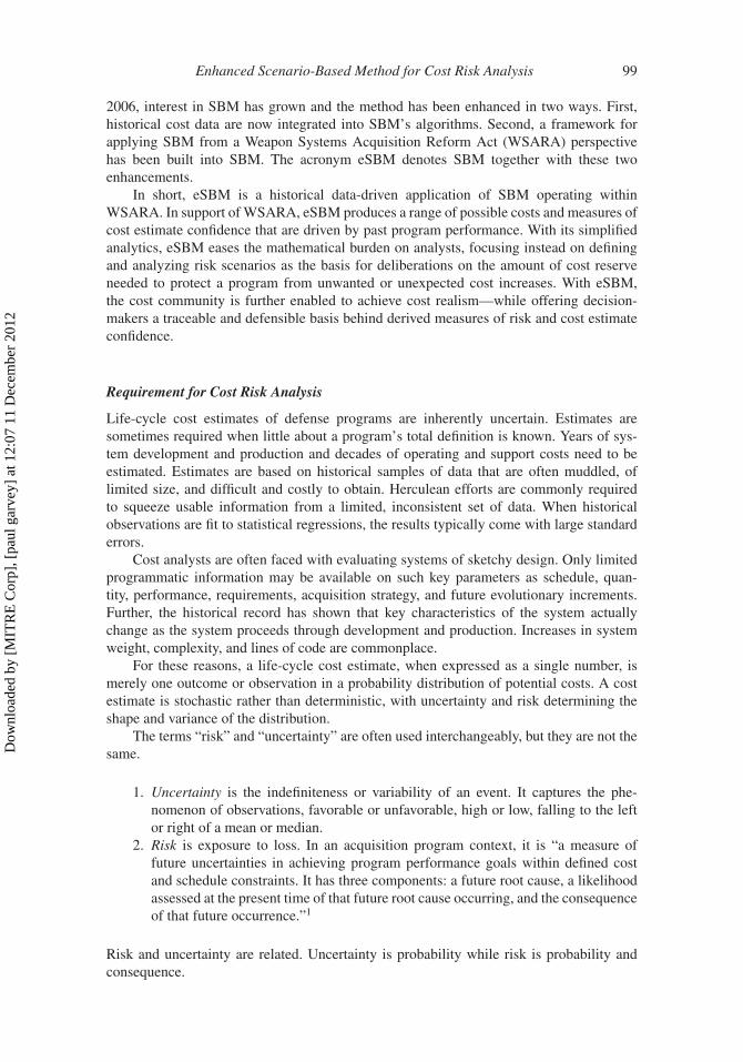
Operational Construct
Figure 19 and Appendix C show benchmark CVs by milestone. The choice of which valuesto use for eSBM or as benchmarks for Monte Carlo simulation will likely depend upon theunique circumstances of a given acquisition program as well as organizational views onissues such as the likelihood of significant volatility in out-year rates of inflation and theeffects on costs of current acquisition initiatives. Keep in mind that low rather than highestimates of CVs have been the norm in the defense cost community.
Summary of Findings
We offer these observations regarding the accuracy of conjectured CV behavior:
● Consistency◦ Conjecture: CVs from ICEs and cost assessments jibe with acquisition experience◦ Finding: Ad hoc observation suggests a pervasive underestimation of CVs in the
international defense community● Tendency to Decline During Acquisition Phase
◦ Conjecture: CVs decrease throughout acquisition lifecycle
Dow
nloa
ded
by [
MIT
RE
Cor
p], [
paul
gar
vey]
at 1
2:07
11
Dec
embe
r 20
12
Enhanced Scenario-Based Method for Cost Risk Analysis 125
1.2
0.8
0.8
0.5
0.9
0.6
0.5
0.4
0.5
0.5
0.3
0.2
0.8 0.8
0.5 0.50.5 0.5
0.30.3 0.3
0.3
0.20.10.0
0.2
0.4
0.6
0.8
1.0
1.2
1.4
Co
effic
ien
t o
f V
aria
tio
n
Estimated CV Bands by Milestone
Quantity
random
TY$ BY$
Quantity
random
TY$ BY$
Quantity
Exogenous
TY$ BY$
Quantity
Exogenous
TY$ BY$
Quantity
Exogenous
TY$ BY$
Quantity
random
TY$ BY$
Milestone A Milestone B Milestone C
Estimated by Analogy
Data => 90sAll data Data => 80s
FIGURE 19 Operational construct (color figure available online).
◦ Finding: Strongly supported● Platform Homogeneity
◦ CVs are equivalent for aircraft, ships, and other platform types◦ Finding: Strongly supported, especially for MS B
● Tendency to Decrease after Normalization◦ CVs decrease when adjusted for changes in quantity and inflation◦ Finding: Strongly supported
● Invariance of Secular Trend◦ CVs steady long-term◦ Finding: Strongly rejected
Recommendations
Based on the forgoing analysis, we offer these recommendations:
● Define the type of CV employed or under discussion.◦ The spreads of max-to-min values of the four types of CVs presented here
(unadjusted and adjusted for quantity and inflation) are simply too large to dootherwise.
● Use a quantity-adjusted, then-year dollar CV for most acquisition programs.◦ That is, regard quantity as exogenous but inflation as random in generating S-
curves.● Define CV benchmark values in terms of bands or ranges at each milestone.
◦ Use of single values presumes a level of knowledge and degree of certainty thatsimply doesn’t exist.
◦ A view of future price stability would argue for the use of lower CVs andinstability for higher.
◦ A belief in the positive effect of structural change due to recent acquisitioninitiatives would argue for lower CVs.
● Exercise prudence in choosing CV benchmarks.◦ Better to err on the side of caution and choose high-end benchmark values until
costs of completed acquisition programs clearly demonstrate lower CGFs andCVs.
Dow
nloa
ded
by [
MIT
RE
Cor
p], [
paul
gar
vey]
at 1
2:07
11
Dec
embe
r 20
12

126 P. R. Garvey et al.
● Choose the high-end of benchmark CV bounds established at Milestone A to supportAoAs and Material Development Decisions.
● Define a “trigger point” or floor for CV estimates, for each milestone, below whicha call-for-explanation will be required.◦ Employ trigger points for both Monte Carlo simulation and eSBM.◦ Base trigger points on confidence intervals for the CVs.
The S-Curve Tool
Under the auspices of the Naval Center for Cost Analysis (NCCA), the S-Curve Toolwas developed to increase the accuracy and robustness of risk and uncertainty analysisin defense cost estimating, while simultaneously decreasing computational burden.19 TheS-Curve Tool, which supports both Monte Carlo simulation and eSBM, allows practitionersto easily and clearly,
● Compare S-curves;● Invoke historical coefficients of variation (CVs) and cost growth factors (CGFs) in
generating S-curves;● Plot alternative point-estimates on an S-curve and easily discern their respective
probabilities of under-run or over-run; and● Generate graphics for decision briefs.
Application of the S-Curve Tool
The S-Curve Tool has been used in a wide variety of cost-analysis applications. Amongnote-worthy usage includes:
● Development by the Department of National Defense, Canada, of an independentcost estimate for Joint Strike Fighter international acquisition, using benchmark CVsin the Tool as the basis for risk and uncertainty analysis;
● Execution of risk and uncertainty analysis for NATO’s Alliance GroundSurveillance System;
● Adoption by the Department of Homeland Security as a standard tool in risk anduncertainty analysis;
● Adoption by the Naval Center for Cost Analysis as both a tool for risk and uncer-tainty analysis and as a basis for comparing historically-derived CVs to those fromin-house ICEs and from program offices cost estimates; and
● Integration of several independent U.S. Navy estimates in comparison to thecontractor’s latest revised estimates for Virginia Class submarines.
Design of the S-Curve Tool
The S-curve was designed with flexibility, robustness, and ease-of-use as conceptual cor-nerstones. Figure 20 shows a flowchart diagram of the NCCA S-Curve Tool Beta Version2.0. With flexibility in mind, the user, upon entering the Tool, chooses among these threeprimary options for conducting risk and uncertainty analysis:
● Empirical◦ The user enters the sample or empirical probability distribution from a Monte
Carlo simulation, as a basis for comparison and analysis;● Parametric
Dow
nloa
ded
by [
MIT
RE
Cor
p], [
paul
gar
vey]
at 1
2:07
11
Dec
embe
r 20
12

Enhanced Scenario-Based Method for Cost Risk Analysis 127
Empirical
(i.e.,a set of outcomes from a
Monte Carlo risk run
Parametric
(i.e.,enhanced Scenario-Based Method (eSBM)
or parameters from external risk analysis)
Point Estimate
(i.e.,risk analysis not yet
done)
Input # of Trials
Select Cost Units for Data
Input Values for Trials
Optional Feature:
Assess empirical data by
overlaying parametric curve
Normal Lognormal
(1) Mean
(2) CV
(1) Mean
(2) Specified Cost (Xp)
with Percentile (p)
Mean Median(1) CV
(2) Specified Cost (Xp)
with Percentile (p)
Users can bring up to two estimates
Are the data Empirical, Parametric, or a Point Estimate?
Normal Lognormal
Estimate
Types of Distributions
Types of Parameters Type of Input
For eSBM,
Xp = XPE & p = αPE
(1) Commodity
(2) Life-cycle phase
(3) Milestone
(4) Inflation
(5) Quantity
(1) Apply CV only
(2) Apply CGF only
(3) Apply CV and CGF
S-Curve
S-Curve
Historical adjustment inputs:
Select how historical
adjustment is applied
to estimate:
Historically adjusted
S-curve is generated
Would you
like to apply historical
adjustments to the
estimate?
YesNo
S-Curve is generated; optional: overlay PDF
FIGURE 20 Flowchart diagram of NCCA S-Curve Tool Beta Version 2.0 (color figureavailable online).
◦ The user enters parameters associated with eSBM or from another external riskanalysis; and
● Point Estimate◦ The user enters a single point estimate and then proceeds to choose, at a later
stage, parameters of the distribution.
Details of the S-Curve Tool
If the estimate type is Empirical, the user inputs the number of trials used in the MonteCarlo simulation, the cost units of the empirical data, such as thousands or millions,and all of the values for the trial runs, with the latter step executed with a couple ofkeystrokes. There is an optional feature to overlay a parametrically-estimated curve, nor-mal or lognormal, on the raw data. This feature has proved of significant practical use inevaluating competing CVs from sources such as a Service Cost Center and program office.
If the estimate type is Parametric, the user defines the type of distribution, either normalor lognormal, and the type of parameters to be used. There are three options for parametrictype:
● Mean and CV;● Mean and Specified Cost (Xp), with the corresponding percentile (p) on the S-curve;
and● CV and Specified Cost (Xp), with the corresponding percentile (p) on the S-curve.20
If the estimate type is a Point Estimate, the user defines the type of distribution, eithernormal or lognormal, and whether the point estimate is a mean or a median value. If thepoint estimate is a median, subsequent application of historical CVs and cost-growth factor
Dow
nloa
ded
by [
MIT
RE
Cor
p], [
paul
gar
vey]
at 1
2:07
11
Dec
embe
r 20
12

128 P. R. Garvey et al.
adjustments pivot on the median in producing an S-curve. In all other cases, Parametric andEmpirical included, the Tool pivots on the mean.
Historical cost growth factors and CVs are binned in the Tool in these categories:type of weapon system, or commodity; acquisition milestone, or phase in the life cycle;inflation, or then-year dollar versus constant-dollar calculations; and quantity or treatmentof variation in acquisition units as exogenous or endogenous to the cost estimate.
After the user selects these inputs, there are three options to apply the historicaladjustments to the estimate:
● CV only, or shaping the S-curve;● CGF only, or shifting the S-curve; and● Both CV and CGF, or shaping and shifting the S-curve.
If users decide not to apply historical adjustments to the estimate, they can proceed withthe base S-curve that was generated.
On-Going Research
On-going research, under the continued aegis of the Naval Center for Cost Analysis, sup-ports both a deep dive and a major expansion of scope into the nature and causes of costgrowth for major weapon-system acquisition programs in the Department of Defense. Datacollection, normalization, and analyses are underway for 400 milestone estimates frommore than 300 MDAPs across the Services. Working with individual SARs in the currenteffort versus SAR Summary Sheets in the initial seminal study will enable CV and CGFcalculations by major appropriation, such as Research, Development, Test, and Evaluation(RDT&E); Procurement; and Military Construction (MILCON). The increase in samplesize will result in improved confidence levels in the calculations. Data for all seven SARcost variance categories are being captured in the current effort and included in a relationaldatabase, all to support demand in the cost community for analyses at this level of granu-larity. We intend to make the emerging database a standard for CV and CGF calculationsin defense cost analysis.
To obtain a copy of the NCCA S-Curve Tool and related documentation, such as theUser Guide and Technical Manual, please visit https://www.ncca.navy.mil/tools/tools.cfm.Detailed values of CVs are available at the same location.
eSBM Case Study
The North Atlantic Treaty Organization (NATO) is acquiring an Alliance GroundSurveillance (AGS) system with the capability of performing persistent surveillanceand reconnaissance over wide areas from high-altitude, long-endurance, Global Hawkunmanned aerial vehicles (UAVs). The Multi-Platform Radar Technology InsertionProgram (MP-RTIP) payload will enable the AGS UAVs to look at what is happeningon the earth’s surface, providing situational awareness before, during, and after NATOoperations, through interfaces with a to-be-designed-and-developed ground segment. Theultimate objective of AGS is “. . . to make soldiers from all NATO countries safer andmore effective when they are deployed on operations.”21 At NATO’s Heads of State andGovernment summit in Lisbon in 2010, President Obama and his 27 national counterpartscollectively reaffirmed the acquisition of AGS as “a top priority” for the Alliance.22
NATO’s SAS-076 Task Group used eSBM to perform risk and uncertainty costanalysis for the AGS acquisition. This was part of a larger effort to generate an ICE on theprogram, the first ever for a weapon system acquisition program conducted by NATO.23
Dow
nloa
ded
by [
MIT
RE
Cor
p], [
paul
gar
vey]
at 1
2:07
11
Dec
embe
r 20
12

Enhanced Scenario-Based Method for Cost Risk Analysis 129
To conduct eSBM, the Task Group needed to:
● Generate a point estimate for acquisition costs,● Identify the position of the point estimate on the S-curve,● Identify and analyze major elements of risk and uncertainty,● Select an appropriate CV ,● Develop scenarios, and● Combine these components into an integrated whole.
Point Estimate and Position on S-Curve
The Task Group employed a number of techniques to estimate the costs of AGS. Theseincluded learning curves, averages of historical data, cost estimating relationships (CERs),and analogies. In many cases, cross checks were developed based on German experi-ence with Eurohawk. Since it is necessary in eSBM to anchor a cost estimate to a pointon a cumulative probability distribution, baseline costs were generated, by design, at themedian, or the 50th percentile. Another choice could have been the mean. Generally, there’sflexibility in choosing either, or perhaps a point in between.24
In the case of AGS, many cost elements were estimated using unit learning curvesor power-function CERs with a multiplicative random error term; that is,
Y = α Qβeε, where Y = unit cost,
Q = lot-midpoint quantity, α and β are parameters (T1 and elasticity) and ε~N (μ, σ 2).
Examples include the wing, fuselage, and empennage of the UAV, and final assembly, inte-gration, test and check out. In these cases, plugging a value of an explanatory variable intothe equation yields an estimated median rather than mean value.25 In other cases, such as forsoftware development where representatives from several participating nations each gener-ated a cost estimate independently, a middle value (median) was selected as the baseline.Moreover, the CERs employed in producing the middle value were themselves median-yielding power-function equations. In other cases, where costs appear normally distributed,the choice or median or mean is a moot point since the values are equal. Examples includesystems engineering and program management, initial spares, and support equipment.
Risk Elements
Next, the Task Group identified these major areas of cost risk and uncertainty:26
● Exchange RateThe AGS contract will be a firm-fixed price direct commercial sale to NorthropGrumman, with a ceiling price denominated in 2007 base-year euros, but with muchof the work done in the United States. Converting from dollars to euros, then, isa major issue. Unfortunately, currency exchange rates are notoriously difficult ifnot impossible to predict accurately and consistently. The projections of Figure 21,using random walk theory, don’t exactly inspire confidence in anyone’s ability tozero in on the future value of the $/C exchange rate.27
Since its introduction roughly a decade ago, the value of the euro has varied froma low of $0.83/C in 2000 to a peak of $1.60/C in 2008, a swing of 93%. Morerecently, during the height of the Greek credit crisis in early 2010, the euro fell to
Dow
nloa
ded
by [
MIT
RE
Cor
p], [
paul
gar
vey]
at 1
2:07
11
Dec
embe
r 20
12

130 P. R. Garvey et al.
FIGURE 21 Projections of euro/dollar exchange rate (color figure available online).
–5%
–4%
–3%
–2%
–1%
0%
1%
2%
3%
4%
5%
An
nu
al
Pe
rce
nt C
ha
ng
e
Inflation and GDP Growth in the Euro Area
Change in Real GDP
Source: raw data from Eurostat
Change in Eu’s
Consumer Price Index
Global financial crisis
1997 1999 2001 2003 2005 2007 2009 2011
FIGURE 22 Inflation and GDP (color figure available online).
$1.18/C. It then returned to pre-crisis levels only to fall once again with the Irishdebt crisis.
● InflationThe ICE team is using a baseline value of 3% inflation per annum for out-yearprojections, weighted according to the relative contributions of the 13 NATO coun-tries participating in the program. However, as Figure 22 shows, inflation in Europe,as measured by the consumer price index, seems to be related to the growth ratein GDP. EU inflation rates fell precipitously during the global financial crisis of2008 but then resumed their secular trend with economic recovery. If the currentrecession in Europe is short-lived, an uptick in inflation during the procurement ofNATO AGS could occur.
● ScheduleThe acquisition of NATO AGS has continually slipped. Further delays will increasethen-year dollar and euro costs due to inflation.
Dow
nloa
ded
by [
MIT
RE
Cor
p], [
paul
gar
vey]
at 1
2:07
11
Dec
embe
r 20
12
Enhanced Scenario-Based Method for Cost Risk Analysis 131
● Software DevelopmentEuropean participants in the AGS program, and Canada, are responsible for groundsegment design, development, and build. Elements of the ground segment includeseveral types of ground vehicles, command and control units, training equipment,and an extensive software development effort. The baseline count of equivalentsource lines of code (ESLOC) is unusually large from a U.S. perspective,28 andincludes no factor for growth.
In the case of AGS, software will be developed in many different countries bymany different companies, possibly using different computer languages and evenoperating systems. Levels of capability maturity model integration (CMMI) cer-tification vary among vendors. Integration of software modules, hardware withsoftware, and AGS with other surveillance assets, such as ASTOR from the U.K.and Global Hawk from the U.S. will all be required. Configuration management andsoftware integration will be major issues. The AGS ICE team uses the average his-torical growth in ESLOC count as a proxy variable for risk for the entire softwaredevelopment effort.
● RadarThe MP-RTIP payload uses advanced electronically scanned array (AESA) tech-nology currently employed on the F/A-18, among other platforms. However, theMP-RTIP development program has experienced significant cost and schedulegrowth which might translate into higher unit production costs.
● International ParticipationThirteen of NATO’s 28 members are funding the acquisition of AGS. Each, in return,demands a fair share of the work. NATO intends to award a contract to NorthropGrumman Integrated Systems Sector International, Inc. (NGISSI), who will havetotal system performance management responsibility and will subcontract work invarious countries, as shown in Figure 23. Developing and producing hardware andsoftware under this work-share constraint in such a multi-cultural, geographically-dispersed environment runs the risk of introducing inefficiencies into the program.
● AffordabilityFitting the desired numbers and capabilities of UAVs and ground-segment ele-ments under NATO’s ceiling price remains a challenge. A few years ago NATO
Northrop Grumman
Integrated Systems
Sector International
2nd Level Subs
Northrop Grumman
Systems Corp
Cassidian (EADS)
Selex Galileo
Kongsberg
3rd Level Sub
Nations
Bulgaria
Czech Republic
Estonia
Latvia
Lithuania
Luxemburg
Romania
Slovakia
Slovenia
FIGURE 23 AGS international contracting (color figure available online).
Dow
nloa
ded
by [
MIT
RE
Cor
p], [
paul
gar
vey]
at 1
2:07
11
Dec
embe
r 20
12

132 P. R. Garvey et al.
and industry envisioned a mixed fleet of manned and unmanned air vehicles to per-form the ground surveillance mission. However, that option was scrapped becauseof cost. Affordability continues to be an issue as many European nations struggleto reduce budget deficits and national debt. Denmark, for example, announced itsintention in 2010 to withdraw from the program because of budget tightening.
Selection of CV
With a point estimate generated and major elements of risk identified, the Task Groupneeded a CV to implement eSBM. NATO, it is important to note, uses the PhasedArmaments Programming System (PAPS) as its acquisition framework. In PAPS, AGSis near what we call a Milestone B decision in the U.S. Further, although AGS is anAlliance rather than a U.S. DoD acquisition program, the prime contractor will be NorthropGrumman, and close to two-thirds of the costs will be incurred in the U.S. The use ofbenchmark CV data from the U.S., then, seems appropriate, especially since none areavailable for NATO acquisitions.
The Task Group selected a MS B CV of 51% based on the full sample of data forquantity-adjusted then-year dollar acquisition outcomes. That is, the Task Group regardedthe quantity of UAVs and ground vehicles as exogenous but the rate of inflation as random,for purposes of generating an S-curve. Given affordability and exchange rate issues, themassive software development effort, and extensive international participation with eachcountry demanding “noble work,” the Task Group judged the higher-end of MS B CVvalues to be appropriate.
Scenarios
The Task Group bundled risks and uncertainties into the scenarios of Figure 24.29
In keeping with the tenets of eSBM, the non-baseline scenarios did not representextreme cases but rather a set of conditions that could easily occur in the future. For exam-ple, the worst imaginable case for the U.S. dollar or the Euro might be a severe devaluation
Baseline
Exchange rate: $1.35/Euro
Inflation: 3% per annum
Quantities: 8 UAVs and 15
ground-segment vehicles
Schedule: contract award by end
of CY2011
91% learning on radar
No impact for building in NATO
environment
Pessimistic
X% deviation in exchange rate
Increase in the rate of inflation of
xxx basis points per annum
No change in quantities
Slip in schedule
Decrease in learning on radar
Increase in SE/PM due to multi
national environment
-
Resource-
Constrained
Quantities decreased to fit
within ceiling price
FIGURE 24 eSBM scenarios for AGS (color figure available online).
Dow
nloa
ded
by [
MIT
RE
Cor
p], [
paul
gar
vey]
at 1
2:07
11
Dec
embe
r 20
12

Enhanced Scenario-Based Method for Cost Risk Analysis 133
of either.30 On the other hand, modest appreciation or depreciation of the dollar or Euro iscertainly plausible, depending upon circumstances.
S-Curve
With a point estimate, CV , and anchored position on the S-curve in hand, eSBM resultswere calculated, with Figure 24 showing results. Costs are not displayed on the x-axis dueto the business-sensitive nature of the information.
Nevertheless, several points of the analysis merit emphasis:
● Not all areas of risk and uncertainty are captured in the scenarios, nor do they need tobe. That is the great advantage of employing an historically-based CV in computingan S-curve. The distribution implicitly captures the totality of events that will influ-ence the cost of the acquisition. A maintained hypothesis, of course, is that historicalvariances will continue to hold.
● The scenarios reflect cost estimates for the events or assumptions they portray.In supporting the NATO AGS Management Agency (NAGSMA) in Brussels, theTask Group estimated and presented costs of each element of risk (e.g., the costimpact of a 50% increase in ESLOC count) within a scenario. The associatedprobabilities for the scenarios were simply read from the S-curve.
● The resource-constrained scenario was regarded as a distinct, separate what-ifdrill. Estimating the risk and uncertainty of changes in acquisition quantity isgenerally beyond the purview of cost analysts. Such changes often result fromCongressional action, which can be hard to predict. The historical CVs were alladjusted for quantity variation; if they weren’t, they would be far higher than theyare.
● The probability of NATO AGS acquisition costs increasing from the baseline tothe pessimistic scenario is roughly one in four or five. Identification and quantifica-tion of this possibility can form the basis of risk-management planning by both theprogram office (NAGSMA) and the prime contractor.
S-Curve Excursion
To demonstrate the consequences of using an inaccurate CV , Figure 25 shows a secondS-curve based on a hypothetical value of 10%.
If the 10% value had been used in the actual analysis, the probability of costs reachingor exceeding the value of the pessimistic scenario would be calculated as only five in onemillion! Yet, to repeat, the parameters used in this scenario are realistic, modest deltasto the baseline. They include what the Task Group regarded as a very slight change inthe exchange rate, a modest increase in the rate of inflation, use of a mean growth factorfor number of equivalent source lines of code, and a percentage increase in the cost ofsystem engineering/program management due to international participation that at leastone member of the team thought was appropriate only if two rather than 14 nations wereinvolved in AGS design, development, and build. In short, the steep S-curve would deceivestakeholders into believing that risk was slight and the probability of significant cost growthminimal.
Specification and adoption of a pessimistic scenario in eSBM, which can easily beadopted in Monte Carlo methodology, too, has the virtue of providing the means with whichto perform a sanity check on the value of the CV . If the resulting S-curve is too steep tobe plausible, then underlying risk and uncertainty distributions for major cost elements
Dow
nloa
ded
by [
MIT
RE
Cor
p], [
paul
gar
vey]
at 1
2:07
11
Dec
embe
r 20
12

134 P. R. Garvey et al.
0%
20%
40%
60%
80%
100%
Estim
ate
d C
um
ula
tiv
e P
ro
ba
bil
ity
Estimated Acquisition Cost in Billions of Then - Year Euros
Estimated Acquisition Cost of NATO AGS
Baseline Scenario
-
Baseline CV of 51%
with 95% Confidence Interval
Mean Median
Pessimistic Scenario
$x.xx per Euro
x% growth in ESLOC
x% learning on MP - RTIP
Cost delta for NATO work
•
•
•
•
•
$1.35 per Euro•
No growth in ESLOC; learning on MRRTIP•
Inflation at 3%; no delta for NATO work•
Inflation at x% per year23% probability
of cost increase
10%CV yields estimate at
99.9995Cum Percentile
FIGURE 25 S-Curve for NATO AGS cost (color figure available online).
must not have been calculated correctly. Chances are that at least one of them in the actualanalysis was too narrow.
Finally, since the mean of a lognormal distribution involves a variance term, use of asteeper S-curve would have resulted in a lower value of expected cost.
Summary
In 2006, the Scenario-Based Method (SBM) was introduced as an alternative to advancedstatistical methods for generating measures of cost risk. Since then, enhancements toSBM have been made. These include integrating historical cost performance data intoSBM’s algorithms and providing a context for applying SBM from a WSARA perspective.Together, these improvements define the enhanced SBM (eSBM)—an historical data-driven application of SBM.
Among other things, eSBM does the following:
● Provides an analytic argument for deriving the amount of cost reserve needed toguard against well-defined “scenarios”;
● Brings the discussion of “scenarios” and their credibility to the decision-makers;this is a more meaningful topic to focus on, instead of statistical abstractions thatsimulation approaches can sometimes create;
● Does not require the use of statistical methods to develop a valid measure of costrisk reserve (this is the non-statistical eSBM);
● Allows percentiles (confidence measures) to be designed into the approach with aminimum set of statistical assumptions;
● Allows percentiles (as well as the mean, median [50th percentile], variance,etc.) to be calculated algebraically in near-real time within a simple spreadsheetenvironment;
● Avoids the requirement to develop probability distribution functions for all theuncertain variables in a WBS, a task that can be time-consuming and hard to justify;
● Captures correlation indirectly in the analysis by the magnitude of the coefficient ofvariation applied in the statistical eSBM;
● Supports traceability and focuses attention on key risk events in the written scenariosthat have the potential to drive cost higher than expected.
Dow
nloa
ded
by [
MIT
RE
Cor
p], [
paul
gar
vey]
at 1
2:07
11
Dec
embe
r 20
12

Enhanced Scenario-Based Method for Cost Risk Analysis 135
In summary, eSBM encourages and emphasizes a careful and deliberative approach to cost-risk analysis. It requires the development of scenarios that represent the program’s “riskstory” rather than a debate about what percentile to select. Time is best spent building thecase arguments for how a confluence of risk events that form a risk scenario might drive theprogram to a particular percentile. This is where the debate and the analysis should center.
Acknowledgments
The Technomics authors kindly acknowledge and deeply appreciate the support of theNaval Center for Cost Analysis, under whose auspices their research was conducted.
Notes
1. “Risk Management Guide for DoD Acquisition, Sixth Edition, August 2006; USD(AT&L),Systems and Software Engineering, Enterprise Development, page 33.
2. The General Theory of Employment, Interest, and Money; Keynes, John Maynard; HarcourtBrace Jovanovich; 1964, page 149.
3. Economic Theory and Operations Analysis, Baumol, William; Prentice-Hall; 1977, page 621.4. Interestingly, use of Monte Carlo simulation is more popular in the U.S. DoD than in the
ministries of defense in other NATO countries where use of sensitivity analysis predominates.5. The original WSARA “80th” percentile requirement has been relaxed numerically to require
an expression and rationale for the actual confidence level used, at whatever percentile, ingenerating the cost estimate.
6. Findings from a RAND study on weapon system cost growth (RAND, 2007) revealed thedistribution of cost growth is approximately lognormal.
7. SAR Summary Sheets are produced annually by the Office of the Undersecretary of Defense(Acquisition, Technology, and Logistics); Acquisition Resources and Analysis.
8. “APBs as we know them today did not start until 1988, and were not incorporated intothe Consolidated Acquisition Reporting System (CARS), [now replaced by the] DefenseAcquisition Management Information Retrieval DAMIR [system] until 1990;” e-mail from thelate Ms. Chris Knoche, USD(AT&L); 25 Feb 2011. Historically (1970s and 1980s), DoD’s SARInstruction 7000.3 indicated that “A Secretary of Defense Decision Memorandum will normallybe the source of . . . cost estimates” in the SAR.
9. Special thanks are due to Mr. John McCrillis of NCCA who enabled the comparison by assem-bling files of OSD ICE memos and program-office cost estimates for many ACAT IC andID programs in the 1990s and 2000s. There was an intersection of 10 acquisition programsbetween Mr. McCrillis’s files and the ones in this study in terms of compatibility of the esti-mates, i.e., same program, same milestone, same quantities, and inclusion of required costdata.
10. Performing what-if drills for alternative development and production quantities and schedules,however, is a legitimate and necessary undertaking.
11. The high-to-low spread in CVs computed using the three methods of quantity adjustment for asample size of 50 ship and submarine acquisition programs at MS B is only 0.02 and 0.04 inbase-year and then-year dollars, respectively.
12. We believe that CVs and S-curves should be estimated and employed with quantity regardedas exogenous but inflation as random. Quantity changes are typically the results of changes inrequirements and departmental or congressional funding decisions. Their impact on cost, wethink, is handled best through what-if drills. For the second term, inflation, more and moreacquisition programs are using non-OSD rates in generating then-year dollar cost estimates.The treatment of outyear inflation rates as a stochastic variable therefore seems appropriate.We recognize that cost-analysis organizations may logically proffer different guidance on thisissue. It’s essential, in any event, to make crystal clear the type of CV employed.
Dow
nloa
ded
by [
MIT
RE
Cor
p], [
paul
gar
vey]
at 1
2:07
11
Dec
embe
r 20
12

136 P. R. Garvey et al.
13. To our knowledge, a test for the equality of k coefficients of variation from lognormal dis-tributions in small samples has not been developed. Hence, we examined the behavior ofthe two components of a CV separately, the mean and standard deviation. In the case ofnormal distributions, see “Confidence Bounds and Hypothesis Tests for Normal DistributionCoefficients of Variation,” Verrill and Johnson, U.S. Department of Agriculture, 2007. In thehypothetical case of a normal distribution for MS B data, the Verrill and Johnson sample-sample procedure does not reject the null hypothesis of equal CVs, at the 10% level ofsignificance.
14. Levene, Howard (1960). “Robust Tests for Equality of Variances,” Ingram Olkin, HaroldHotelling, et al. Stanford University Press, pp. 278–292. Details of the test results are availablefrom the authors.
15. Average annual rate of inflation during a presidency, as measured by the Consumer Price Index.Arguably, inflation for defense was higher.
16. Because of long profiles for expenditures of TOA (seven years for ships, for example), a blipupward in inflation in one year perturbed not only an acquisition program’s budget in that yearbut in many years previously and subsequently, too, thus amplifying the problem.
17. A paucity of data did not allow use of the same platform categories as for Milestone B.18. These results are . . . “not surprising. The F-test is closely tied to the assumption of data normal-
ity. It is not reliable if the distribution of data is significantly non-normal. Alternatively, Levene’stest makes no distributional assumptions, but tends to favor the null unless the counterevidenceis strong.” Comment from Dr. Steve Book, Jan. 2012.
19. The S-Curve Tool was briefed at 44th annual Department of Defense Cost AnalysisSymposium (DODCAS), February, 2011; the joint Society of Cost Estimating and Analysis(SCEA)/International Society of Parametric Analysts (ISPA) conference, June, 2011; and the45th annual DODCAS, February, 2012.
20. There are other ways to define a parametric curve, such as use of two percentages with twospecified point values, but this feature is not implemented in beta version 2.0 of the Tool.
21. Mr. Anders Fogh Rasmussen, Secretary General of NATO; 22 June 2010.22. Lisbon, Portugal, 19 and 20 November, 2010.23. The Systems Analysis and Studies (SAS) Task Group 076 is chaired by Dr. Flynn, and con-
sists of representatives from Sweden, a dozen NATO countries, and OCCAR (Organisationconjointe de coopération en matière d’armement), a European armaments agency. Members ofthe NATO AGS ICE team are Dr. Brian Flynn, Dr. Paul Desmier, Mr. Walter Boos, Mr. JoachimSchotten, Mr. Philippe Lacheret, Mr. Murat Cakmak, Mr. Renzo Chiomento, Dr. Dagfinn Vatne,and Ms. Solveig Krey.
24. The sum of the medians (WBS elements) is not generally equal to the median of the sum (totalcost).
25. Goldberger, Arthur S., “The Interpretation and Estimation of Cobb-Douglas Functions,”Econometrica, Vol. 35, July–October, 1968, pp. 464–472. “. . . the standard specification andapproach to estimation shift attention, apparently unwittingly, from the mean to the median as ameasure of central tendency.”
26. Areas of risk were identified based on general knowledge of defense acquisition programsand the discipline of international economics, site visits to Northrop Grumman’s InternationalProgram Office in Florida and to NATO’s AGS Management Agency in Brussels, and on meet-ings with other key AGS acquisition officials, including the Chairman of the Board of Directorsof the NATO AGS Management Organization.
27. Projections are from Dr. Paul Desmier of the Department of National Defense, Canada.28. Unlike software for Global Hawk in the U.S., AGS includes software for not only the sensor data
collection element (the UAV, sensor and control stations), but also for the user exploitation ele-ments (mobile and transportable ground stations) and a support segment (trainers, maintenanceequipment, etc). In the U.S. environment, the operational exploitation and use of the collectedISR data is performed outside of the Global Hawk system (through the Distributed CommonGround Systems), while for NATO the AGS system will need to include this essential part aswell.
29. Data that might be construed as business sensitive are omitted from the display.
Dow
nloa
ded
by [
MIT
RE
Cor
p], [
paul
gar
vey]
at 1
2:07
11
Dec
embe
r 20
12

Enhanced Scenario-Based Method for Cost Risk Analysis 137
30. Pundits in Europe and the U.S. speculated in February 2010, for example, that the EuropeanUnion, and the Euro, might not survive. Other pundits project financial Armageddon for theU.S. because of our enormous direct national debt ($14 trillion) and unfunded liabilities forSocial Security, Medicare, and other entitlement programs (another $50 trillion).
References
Arena, M. V., et al. (2006). Impossible Certainty: Cost Risk Analysis for Air Force Systems. ProjectAir Force. The RAND Corporation.
Garvey, P. R. (2000). Probability Methods for Cost Uncertainty Analysis: A Systems EngineeringPerspective. New York, NY: Marcel Dekker, Inc., Taylor & Francis Group, Chapman-Hall/CRCPress.
Garvey, P. R. (2008). A Scenario-Based Method for Cost Risk Analysis. Journal of Cost Analysisand Parametrics, 1, 65–76.
General Accountability Office (GAO), (2009). Cost Estimating and Assessment Guide.NASA. Cost Estimating Handbook. (2008). National Aeronautics and Space Administration,
Comptroller, Washington, D.C.Public Law 111–23. (2009). Weapon Systems Acquisition Reform Act of 2009. May 22, 2009.Superintendent of Documents, U.S. Govenment Printing Office, Washington, D.C. 20402.Young, P. H. (1995). A Generalized Probability Distribution for Cost/Schedule Uncertainty in Risk
Assessment. Proceedings of the 1995 Western MultiConference on Business/MIS SimulationEducation, The Society for Computer Simulation, San Diego, California.
Younossi, O., et al. 2007. Is Weapon System Cost Growth Increasing?: A Quantitative Assessment ofCompleted and Ongoing Programs, The RAND Corporation. ISBN 978-0-8330-4135-7.
United States Air Force, Air Force Cost Analysis Agency. (2007). Cost Risk and Uncertainty AnalysisHandbook (CRUH). Deputy Assistant Secretary of the Air Force, Cost and Economics; Pentagon,Washington, D.C.
About the Authors
Paul R. Garvey is Chief Scientist for the Center for Acquisition and Systems Analysis – aDivision of The MITRE Corporation. He has nearly 30 years of experience in systems costanalysis, uncertainty analysis, and in the application of risk-decision analytic methods to avariety of problems in the federal government.
He is the author of over 25 peer-reviewed publications and three textbooks: ProbabilityMethods for Cost Uncertainty Analysis, 2000, Analytical Methods for Risk Management,2008, and Advanced Risk Analysis in Engineering Enterprise Systems, 2012. These worksare from Chapman-Hall/CRC-Press, Taylor & Francis Group.
Dr. Garvey has an A.B. and M.Sc. in pure and applied mathematics from BostonCollege and Northeastern University. He earned a Ph.D. in engineering systems risk analy-sis and decision theory from Old Dominion University (ODU) and was awarded a doctoraldissertation medal from the faculty of the College of Engineering.
Brian J. Flynn is a Technomics Senior Cost Analyst Brian J. Flynn is based at thefirm’s Arlington, Virginia, headquarters where he supports national security efforts and,more specifically, the Naval Center for Cost Analysis, NCCA.
Before joining the firm in 2012, Dr. Flynn worked in NCCA as a plank owner andmore recently as Special Assistant to the Deputy Assistant Secretary of the Navy (Cost andEconomics). He served simultaneously as Study Director and U.S. DoD representative ofa NATO/Partnership for Peace task group on independent cost estimating and capabilityportfolio analysis. A recognized leader in the international defense community, Dr. Flynnreceived the Department of the Navy’s Distinguished Civilian Service Award, the highest
Dow
nloa
ded
by [
MIT
RE
Cor
p], [
paul
gar
vey]
at 1
2:07
11
Dec
embe
r 20
12

138 P. R. Garvey et al.
honorary award the Secretary of the Navy can confer on a civilian employee, as well as theSuperior Civilian Service Award and the Meritorious Civilian Service Award.
Dr. Flynn holds a Ph.D. in Economics, with distinction, from Georgetown Universityand M.A. and B.A. degrees in Economics from Virginia Polytechnic Institute and StateUniversity.
Most importantly of all, Dr. Flynn has undying pride in his service, over a generationago, in the United States Marine Corps. Semper Fidelis.
Peter J. Braxton is a Senior Cost Analyst and Technical Officer at Technomics, Inc.,where he currently supports the Naval Center for Cost Analysis (NCCA) on data collec-tion and cost research efforts, and Defense Acquisition University (DAU) on curriculumdevelopment.
He is a Certified Cost Estimator/Analyst (CCEATM) and currently serves as Bodyof Knowledge Chair for the the International Cost Estimating and Analysis Association(ICEAA). He was named the Society of Cost Estimating and Analysis (SCEA) 2007Estimator of the Year for contributions in Education. He is the managing editor for devel-opment and maintenance of the acclaimed Cost Estimating Body of Knowledge (CEBoK®)and its predecessor, Cost Programmed Review Of Fundamentals (CostPROF). He served asSCEA’s Training Chair from 2004 to 2009 and as Training Track chair for nine consecutiveSCEA international conferences. He has taught extensively at government, corporate, andsociety training events throughout the United States, Europe, and Australia.
He holds an AB in Mathematics from Princeton University and an M.S. in AppliedScience (Operations Research) from the College of William and Mary. He is lead author orco-author of over two dozen professional papers on cost, risk, and Cost As an IndependentVariable (CAIV), including three SCEA Best Paper winners. This is his first journal article.
Richard C. Lee received his B.S. in Mechanical Engineering in 2007 from VirginiaPolytechnic Institute and State University. He joined the Advanced Vehicle DynamicsLaboratory at the same institution and started his graduate studies on modeling and sim-ulation of terrain profile models using numerical methods and vehicle dynamics. Hereceived his M.S. in Mechanical Engineering in the spring of 2009. He is a memberof the International Cost Estimating and Analysis Association (ICEAA) (formerly theSociety of Cost Estimating and Analysis (SCEA)), the American Society of MechanicalEngineers (ASME), and the Institute for Operations Research and the ManagementSciences (INFORMS). A Cost Analyst at Technomics, Inc., he has supported the Officeof the Secretary of Defense, Cost Assessment and Program Evaluation (OSD CAPE), theOffice of the Deputy Assistant Secretary of the Army for Cost and Economics (ODASA-CE), the Naval Center for Cost Analysis (NCCA), and the Naval Sea Systems Command(NAVSEA) 05C on projects spanning Earned Value Management (EVM) analysis, data col-lection and cost research, risk analysis, and estimate development. He is a Certified CostEstimator/Analyst.
Appendix A
Percentiles of the Standard Normal Random Variable
The tables below are values of the cumulative distribution function of the standard normalrandom variable Z, where Z ∼ N(0, 1). The columns with three-digits represent values for Zdenoted by the small letter z. The columns with the eight-digits are equal to the probabilitygiven by the integral below.
Dow
nloa
ded
by [
MIT
RE
Cor
p], [
paul
gar
vey]
at 1
2:07
11
Dec
embe
r 20
12

Enhanced Scenario-Based Method for Cost Risk Analysis 139
TABLE A-1 Percentiles of the standard normal values
0.00 0.5000000 0.21 0.5831661 0.42 0.6627572 0.63 0.73565280.01 0.5039894 0.22 0.5870644 0.43 0.6664021 0.64 0.73891380.02 0.5079784 0.23 0.5909541 0.44 0.6700314 0.65 0.74215400.03 0.5119665 0.24 0.5948348 0.45 0.6736448 0.66 0.74537320.04 0.5159535 0.25 0.5987063 0.46 0.6772419 0.67 0.74857120.05 0.5199389 0.26 0.6025681 0.47 0.6808225 0.68 0.75174780.06 0.5239223 0.27 0.6064198 0.48 0.6843863 0.69 0.75490300.07 0.5279032 0.28 0.6102612 0.49 0.6879331 0.70 0.75803640.08 0.5318814 0.29 0.6140918 0.50 0.6914625 0.71 0.76114800.09 0.5358565 0.30 0.6179114 0.51 0.6949743 0.72 0.76423760.10 0.5398279 0.31 0.6217195 0.52 0.6984682 0.73 0.76730500.11 0.5437954 0.32 0.6255158 0.53 0.7019441 0.74 0.77035010.12 0.5477585 0.33 0.6293000 0.54 0.7054015 0.75 0.77337270.13 0.5517168 0.34 0.6330717 0.55 0.7088403 0.76 0.77637280.14 0.5556700 0.35 0.6368306 0.56 0.7122603 0.77 0.77935010.15 0.5596177 0.36 0.6405764 0.57 0.7156612 0.78 0.78230460.16 0.5635595 0.37 0.6443087 0.58 0.7190427 0.79 0.78523620.17 0.5674949 0.38 0.6480272 0.59 0.7224047 0.80 0.78814470.18 0.5714237 0.39 0.6517317 0.60 0.7257469 0.81 0.79103000.19 0.5753454 0.40 0.6554217 0.61 0.7290692 0.82 0.79389200.20 0.5792597 0.41 0.6590970 0.62 0.7323712 0.83 0.7967307
0.84 0.7995459 1.05 0.8531409 1.26 0.8961653 1.47 0.92921910.85 0.8023375 1.06 0.8554277 1.27 0.8979576 1.48 0.93056330.86 0.8051055 1.07 0.8576903 1.28 0.8997274 1.49 0.93188790.87 0.8078498 1.08 0.8599289 1.29 0.9014746 1.50 0.93319280.88 0.8105704 1.09 0.8621434 1.30 0.9031995 1.51 0.93447830.89 0.8132671 1.10 0.8643339 1.31 0.9049020 1.52 0.93574450.90 0.8159399 1.11 0.8665004 1.32 0.9065824 1.53 0.93699160.91 0.8185888 1.12 0.8686431 1.33 0.9082408 1.54 0.93821980.92 0.8212136 1.13 0.8707618 1.34 0.9098773 1.55 0.93942920.93 0.8238145 1.14 0.8728568 1.35 0.9114919 1.56 0.94062000.94 0.8263912 1.15 0.8749280 1.36 0.9130850 1.57 0.94179240.95 0.8289439 1.16 0.8769755 1.37 0.9146565 1.58 0.94294660.96 0.8314724 1.17 0.8789995 1.38 0.9162066 1.59 0.94408260.97 0.8339768 1.18 0.8809998 1.39 0.9177355 1.60 0.94520070.98 0.8364569 1.19 0.8829767 1.40 0.9192433 1.61 0.94630110.99 0.8389129 1.20 0.8849303 1.41 0.9207301 1.62 0.94738391.00 0.8413447 1.21 0.8868605 1.42 0.9221961 1.63 0.94844931.01 0.8437523 1.22 0.8887675 1.43 0.9236414 1.64 0.94949741.02 0.8461358 1.23 0.8906514 1.44 0.9250663 1.65 0.95052851.03 0.8484950 1.24 0.8925122 1.45 0.9264707 1.66 0.95154281.04 0.8508300 1.25 0.8943502 1.46 0.9278549 1.67 0.9525403
(continued)
Dow
nloa
ded
by [
MIT
RE
Cor
p], [
paul
gar
vey]
at 1
2:07
11
Dec
embe
r 20
12

140 P. R. Garvey et al.
TABLE A-1 Percentiles of the standard normal values (continued)
1.68 0.9535214 1.89 0.9706211 2.10 0.9821356 2.31 0.98955591.69 0.9544861 1.90 0.9712835 2.11 0.9825709 2.32 0.98982961.70 0.9554346 1.91 0.9719335 2.12 0.9829970 2.33 0.99009691.71 0.9563671 1.92 0.9725711 2.13 0.9834143 2.40 0.99180251.72 0.9572838 1.93 0.9731967 2.14 0.9838227 2.50 0.99379031.73 0.9581849 1.94 0.9738102 2.15 0.9842224 2.60 0.99533881.74 0.9590705 1.95 0.9744120 2.16 0.9846137 2.70 0.99653301.75 0.9599409 1.96 0.9750022 2.17 0.9849966 2.80 0.99744481.76 0.9607961 1.97 0.9755809 2.18 0.9853713 2.90 0.99813411.77 0.9616365 1.98 0.9761483 2.19 0.9857379 3.00 0.99865001.78 0.9624621 1.99 0.9767046 2.20 0.9860966 3.10 0.99903231.79 0.9632731 2.00 0.9772499 2.21 0.9864475 3.20 0.99931281.80 0.9640697 2.01 0.9777845 2.22 0.9867907 3.30 0.99951651.81 0.9648522 2.02 0.9783084 2.23 0.9871263 3.40 0.99966301.82 0.9656206 2.03 0.9788218 2.24 0.9874546 3.50 0.99976731.83 0.9663751 2.04 0.9793249 2.25 0.9877756 3.60 0.99984091.84 0.9671159 2.05 0.9798179 2.26 0.9880894 3.70 0.99989221.85 0.9678433 2.06 0.9803008 2.27 0.9883962 3.80 0.99992761.86 0.9685573 2.07 0.9807739 2.28 0.9886962 3.90 0.99995191.87 0.9692582 2.08 0.9812373 2.29 0.9889894 4.00 0.99996831.88 0.9699460 2.09 0.9816912 2.30 0.9892759 5.00 0.9999997
P(Z ≤ z) =z∫
− ∞
1√2π
e−y2/2dy.
Since Z ∼ N (0, 1) the following is true; P (Z ≤ −z) = P (Z > z) = 1 − P (Z ≤ z).
Example Computations
1. P(Z ≤ z = −0.525) = P(Z > z = 0.525) = 1 − P(Z ≤ z = 0.525) = 1 − 0.70 = 0.302. P(Z ≤ z = −0.675) = P(Z > z = 0.675) = 1 − P(Z ≤ z = 0.675) = 1 − 0.75 = 0.253. P(Z ≤ z = 0.525) = 0.70
Appendix B
The Lognormal Distribution
The lognormal probability distribution has broad applicability in engineering, economics,and cost analysis. In engineering, the failure rates of mechanical or electrical componentsoften follow a lognormal distribution. In economics, the random variation between the pro-duction cost of goods to capital and labor costs is frequently modeled after the lognormaldistribution. In cost analysis, the lognormal often approximates the probability distributionof a program’s total cost (Young, 1995; Garvey, 2000).
If X is a nonnegative random variable and ln X follows the normal distribution, thenX is said to have a lognormal distribution. The lognormal probability density function isgiven by
Dow
nloa
ded
by [
MIT
RE
Cor
p], [
paul
gar
vey]
at 1
2:07
11
Dec
embe
r 20
12
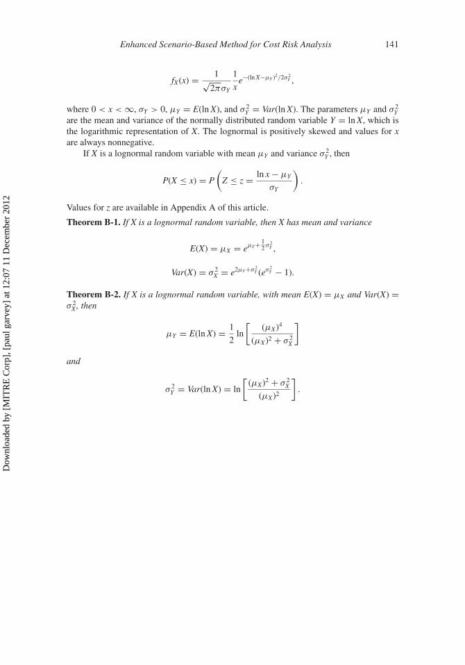
Enhanced Scenario-Based Method for Cost Risk Analysis 141
fX(x) = 1√2πσY
1
xe−(ln X−μY )2/2σ 2
Y ,
where 0 < x < ∞, σY > 0, μY = E(ln X), and σ 2Y = Var(ln X). The parameters μY and σ 2
Yare the mean and variance of the normally distributed random variable Y = ln X, which isthe logarithmic representation of X. The lognormal is positively skewed and values for xare always nonnegative.
If X is a lognormal random variable with mean μY and variance σ 2Y , then
P(X ≤ x) = P
(Z ≤ z = ln x − μY
σY
).
Values for z are available in Appendix A of this article.
Theorem B-1. If X is a lognormal random variable, then X has mean and variance
E(X) = μX = eμY+ 12 σ 2
Y ,
Var(X) = σ 2X = e2μY+σ 2
Y (eσ 2Y − 1).
Theorem B-2. If X is a lognormal random variable, with mean E(X) = μX and Var(X) =σ 2
X , then
μY = E(ln X) = 1
2ln
[(μX)4
(μX)2 + σ 2X
]
and
σ 2Y = Var(ln X) = ln
[(μX)2 + σ 2
X
(μX)2
].
Dow
nloa
ded
by [
MIT
RE
Cor
p], [
paul
gar
vey]
at 1
2:07
11
Dec
embe
r 20
12

142 P. R. Garvey et al.
Appendix C
CVs for Estimates of Total Program Acquisition Cost
Milestone Milestone MilestoneA B C
CV Calculation and DefinitionUsing Complete Sample of DataQuantity Random (Unadjusted for Qty �)
Then-year dollars 1.20 0.87 0.53Base-year dollars 0.82 0.63 0.45
Quantity Exogenous (Adjusted for Qty �)Then-year dollars 0.76 0.51 0.26Base-year dollars 0.52 0.36 0.19
CV Calculation and DefinitionUsing Data from 1980 and LaterQuantity Random (Unadjusted for Qty �)
Then-year dollars 0.84 0.69 0.53Base-year dollars 0.85 0.65 0.45
Quantity Exogenous (Adjusted for Qty �)Then-year dollars 0.54 0.40 0.26Base-year dollars 0.56 0.37 0.19
CV Calculation and DefinitionUsing Data from 1990 and LaterQuantity Random (Unadjusted for Qty �)
Then-year dollars 0.77 0.53 0.29Base-year dollars 0.76 0.51 0.25
Quantity Exogenous (Adjusted for Qty �)Then-year dollars 0.50 0.33 0.16Base-year dollars 0.50 0.30 0.11
Dow
nloa
ded
by [
MIT
RE
Cor
p], [
paul
gar
vey]
at 1
2:07
11
Dec
embe
r 20
12