ENHANCED FEM-DBEM

APPROACH FOR FATIGUE

CRACK-GROWTH

SIMULATION

Venanzio Giannella

Unione Europea UNIVERSITÀ DEGLI

STUDI DI SALERNO

FONDO SOCIALE EUROPEO Programma Operativo Nazionale 2000/2006

“Ricerca Scientifica, Sviluppo Tecnologico, Alta Formazione”

Regioni dell’Obiettivo 1 – Misura III.4

“Formazione superiore ed universitaria”

Department of Industrial Engineering

Ph.D. Course in Mechanical Engineering

(XVI Cycle-New Series, XXX Cycle)

ENHANCED FEM-DBEM APPROACH FOR

FATIGUE CRACK-GROWTH SIMULATION

Supervisor Ph.D. student

Prof. Roberto Guglielmo Citarella Venanzio Giannella

Scientific Referee

Prof. Renato Esposito

Ph.D. Course Coordinator

Prof. Ernesto Reverchon

List of publications

R. Citarella, V. Giannella, M. Lepore, DBEM crack propagation for nonlinear

fracture problems, Frattura ed Integrità Strutturale, 34 (2015) 514-523; DOI:

10.3221/IGF-ESIS.34.57.

R. Citarella, V. Giannella, E. Vivo, M. Mazzeo, FEM-DBEM approach for

crack propagation in a low pressure aeroengine turbine vane segment,

Theoretical and Applied Fracture Mechanics, Volume 86, Part B, December

2016, Pages 143-152, DOI: 10.1016/j.tafmec.2016.05.004.

R. Citarella, V. Giannella, M. Lepore, G. Dhondt, Dual boundary element

method and finite element method for mixed-mode crack propagation

simulations in a cracked hollow shaft, DOI: 10.1111/ffe.12655.

V. Giannella, J. Fellinger, M. Perrella, R. Citarella, Fatigue life assessment in

lateral support element of a magnet for nuclear fusion experiment

“Wendelstein 7-X”, Engineering Fracture Mechanics, Volume 178, 1 June

2017, Pages 243-257, DOI: 10.1016/j.engfracmech.2017.04.033.

R.C. Wolf, V. Giannella, et alii., Major results from the first plasma campaign

of the Wendelstein 7-X stellarator, DOI: 10.1088/1741-4326/aa770d.

V. Giannella, M. Perrella, R. Citarella, Efficient FEM-DBEM coupled

approach for crack propagation simulations, Theoretical and Applied Fracture

Mechanics, Volume 91, October 2017, Pages 76-85, DOI:

10.1016/j.tafmec.2017.04.003.

R. Citarella, V. Giannella, M. Lepore, J. Fellinger, FEM-DBEM approach to

analyse crack scenarios in a baffle cooling pipe undergoing heat flux from the

plasma, 2017, AIMS Journal 4(2):391-412, 2017, DOI:

10.3934/matersci.2017.2.391.

6

V. Giannella, R. Citarella, J. Fellinger, R. Esposito, LCF assessment on heat

shield components of nuclear fusion experiment “Wendelstein 7-X” by critical

plane criteria, Procedia Structural Integrity 8 (2018) 318-331.

I

Summary

Summary ......................................................................................................... I

List of figures ............................................................................................... III

List of tables ................................................................................................. VI

Abstract ....................................................................................................... VII

Introduction .................................................................................................... 1

I General aspects ........................................................................................ 1

II Fracture Mechanics................................................................................. 3

III Numerical analyses ............................................................................... 5

IV Boundary Element Method (BEM) and Dual BEM .............................. 6

V Description of Thesis.............................................................................. 8

Chapter I FEM-DBEM approaches to Fracture Mechanics ......................... 11

I.1 Introduction ......................................................................................... 11

I.2 Superposition principle for Linear Elastic Fracture Mechanics .......... 13

I.3 FEM-DBEM coupled approaches ....................................................... 14

I.4 Crack-growth criteria .......................................................................... 16

I.4.1 SIF evaluation .............................................................................. 16

I.4.2 Kink angle assessment ................................................................. 18

I.4.3 Crack-Growth Rate (CGR) assessment ........................................ 20

I.4.4 Mixed-mode crack-growth ........................................................... 21

Chapter II FEM-DBEM benchmark ............................................................ 23

II.1 Introduction ....................................................................................... 23

II.2 Problem description ........................................................................... 23

II.3 DBEM modelling .............................................................................. 26

II.4 FEM modelling .................................................................................. 27

II

II.5 FEM-DBEM modelling ..................................................................... 29

II.6 Results ............................................................................................... 31

II.7 Remarks ............................................................................................. 35

Chapter III Aeroengine turbine FEM-DBEM application ........................... 37

III.1 Introduction ...................................................................................... 37

III.2 Problem description .......................................................................... 37

III.3 FEM modelling ................................................................................. 38

III.4 Metallographic post-mortem investigation ....................................... 40

III.5 DBEM submodelling approach ........................................................ 41

III.6 Results .............................................................................................. 45

III.7 Remarks ............................................................................................ 49

Chapter IV FEM-DBEM application on Wendelstein 7-X structure .......... 51

IV.1 Introduction ...................................................................................... 51

IV.2 Problem description ......................................................................... 51

IV.3 FEM modelling ................................................................................ 56

IV.4 DBEM modelling ............................................................................. 58

IV.5 Fatigue load spectra .......................................................................... 61

IV.6 Results .............................................................................................. 63

IV.7 Remarks............................................................................................ 70

Conclusions .................................................................................................. 71

References .................................................................................................... 73

Nomenclature ............................................................................................... 78

List of figures

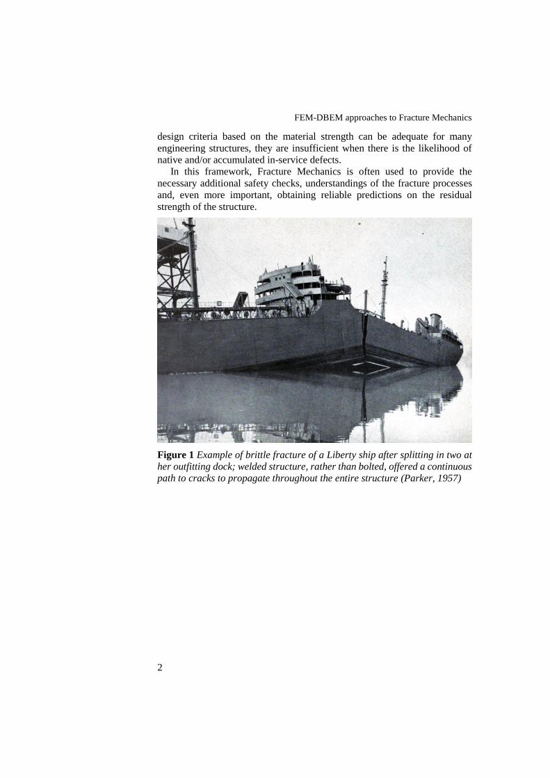
Figure 1 Example of brittle fracture of a Liberty ship after splitting in two at

her outfitting dock; welded structure, rather than bolted, offered a continuous

path to cracks to propagate throughout the entire structure (Parker, 1957) . 2 Figure 2 Example of fatigue crack-growth in a turbofan engine (Pratt &

Whitney JT8D) occurred during the take-off roll; a fan disk penetrated the left

aft fuselage determining two fatalities (www.wikipedia.it). ........................... 3 Figure 3 (a) Traditional designing philosophy vs. (b) Damage Tolerance

design philosophy. .......................................................................................... 4 Figure 4 Example of a 2D model via (a) FEM and (b) BEM. ....................... 6 Figure 5 Example of (a) FEM and (b) BEM models of a reinforced curved

fuselage panel (Aliabadi, 2002) ..................................................................... 6

Figure I. 1 Example of a (a) FEM and a (b) DBEM submodelling of a gear

tooth with a crack (2D problem). ................................................................. 12 Figure I. 2 Superposition principle applied to a fracture problem; 𝜎0 is the

pre-existing stress field generated by the applied prescribed conditions, etc.

...................................................................................................................... 13 Figure I. 3 Different approaches for the selection of the DBEM submodel

loading conditions for a gear tooth with a crack: (a) Fixed Displacement

(FD); (b) Fixed Load (FL); (c) Loaded Crack (LC). ................................... 15 Figure I. 4 Closed path around crack tip (Wilson, 1976). .......................... 17 Figure I. 5 Schematic plot of the typical 𝑑𝑎𝑑𝑁 vs. ∆𝐾 relationship; the Paris

law is calibrated to model the linear part of the graph. ............................... 20

Figure II. 1 Drawings of the (a) shaft with highlight of the crack and fillet

radii, (b) hub with the dotted red line representing the loading application

zone. ............................................................................................................. 24 Figure II. 2 Considered load cases: (a) ‘‘coupled”, (b) ‘‘shear” and (c)

‘‘torque”. ..................................................................................................... 25 Figure II. 3 DBEM uncracked model with close‐up of the remeshed area

surrounding the crack insertion point and details of the initial crack

geometry with J‐paths along the crack front (purple) for the J‐integral

computation. ................................................................................................. 27 Figure II. 4 ZENCRACK (ZC)/ABAQUS uncracked model with highlight on

the brick elements that are subsequently substituted with crack blocks. ..... 28

IV

Figure II. 5 CRACKTRACER3D (CT3D)/CalculiX uncracked model with

the subsequent cracked mesh and details of the crack. ................................ 29 Figure II. 6 (a) FEM and DBEM submodel used for the FEM-DBEM

approach; (b) DBEM submodel after that the crack has been inserted and

loaded. .......................................................................................................... 31 Figure II. 7 SIFs calculated by the considered methodologies for load

cases: (a) coupled, (b) shear and (c) torque; X-axis is the normalised

abscissa drawn along crack front................................................................. 32 Figure II. 8 Crack size definitions. .............................................................. 34 Figure II. 9 Plots of crack sizes vs. total fatigue cycles for the load cases of:

(a) coupled; (b) shear; (c) torque. ................................................................ 35

Figure III. 1 Material properties vs. temperature for the considered

superalloy: Young’s modulus (a), thermal expansion coefficient (b) and

Poisson’s ratio (c). ....................................................................................... 39 Figure III. 2 FEM model: (a) thermal scenario and (b) cyclic symmetry

boundary conditions (highlighted in green). ................................................ 40 Figure III. 3 Tangential displacements (a) and max principal stresses (b) on

the statoric segment. ..................................................................................... 40 Figure III. 4 Segment affected by fatigue failure: (a) damaged airfoil with

highlight (yellow arrows) of the undesired double radius on the trailing edge;

(b) estimated initial crack front (red line). ................................................... 41 Figure III. 5 (a) Realistic engine mission profile and (b) its simplified profile

adopted in this work. .................................................................................... 42 Figure III. 6 Considered loading strategies for DBEM analyses: (a) LC and

(b) FD; model for LC comprises the self-equilibrated load on the crack face

elements and few constraints to prevent rigid body motion; model for FD

comprises temperature on all the elements and displacement field on all the

cut surface elements. .................................................................................... 44 Figure III. 7 Max principal stresses before crack introduction on the two

DBEM submodels used for FD approach; highlight of the crack insertion

position. ........................................................................................................ 44 Figure III. 8 Von Mises stresses [psi] for the initial cracked FD (a) and LC

(b) models, with close-up of the cracked area (cutting sphere radius R = 1

in.). ............................................................................................................... 46 Figure III. 9 Different meshes on the crack face, as used for the convergence

study. ............................................................................................................ 47 Figure III. 10 Different meshes on the crack face, as used for the convergence

study between (a) LC and (b) FD methods; X axis is the normalised abscissa

drawn along the crack front. ........................................................................ 47 Figure III. 11 Comparison on crack sizes vs. cycles plots for small and large

submodels and both the methodologies: (a) LC and (b) FD. ....................... 48

Figure IV. 1 (a) Modular-type stellarator Wendelstein 7-X; (b) Hot plasma

confined by EM field generated by the coils; (c) FEM assembly of one-fifth of

V

the magnet system of W7-X; (d) W7-X magnet system: FEM detail of a half

module with the LSEs; highlights on the investigated LSE-05. .................... 54 Figure IV. 2 LSE-05: real component with highlight of discovered surface

cracks; continuous circle (red line) surrounding the most critical (and

modelled) crack. ........................................................................................... 55 Figure IV. 3 Von Mises stresses [Pa], related to the load case with EM field

of 3 T “HJ”, on the: (a) FEM global model, (b) first FEM LSE-05 submodel,

(c) furtherly reduced FEM submodel. Red arrow in (a) pointing out the

submodelled LSE-05 in (b). Dashed red square in (b) representing the area

that has been furtherly refined in (c). ........................................................... 57 Figure IV. 4 (a) FEM submodel and (b) DBEM uncracked submodel (the red

dot is the crack insertion point), obtained by a Boolean subtraction with a

sphere of radius 0.11 m. ............................................................................... 59 Figure IV. 5 DBEM cracked submodel with highlight of the different modelled

zones. ............................................................................................................ 59 Figure IV. 6 DBEM submodel loaded with different BCs: either (a)

displacements (FD) or (c) tractions (FL) applied on cut surfaces; (b) tractions

applied on the crack faces (LC). .................................................................. 60 Figure IV. 7 Schematic loading history due to EM forces. ......................... 62 Figure IV. 8 (a) DBEM crack (deformed shape) with the applied tractions (in

orange) for the LC approach; (b) crack sizes definition with J-paths along

crack front (in purple). ................................................................................. 64 Figure IV. 9 (a) Von Mises stress scenario for LC approach; initial crack

configuration and load case iii; (b) close up of the von Mises stress scenario

in the crack surroundings for LC approach; initial crack configuration and

load case iii. ................................................................................................. 64 Figure IV. 10 Von Mises stress scenario from FD/FL approach; initial crack

configuration and load case iii..................................................................... 65 Figure IV. 11 SIF values along the crack front for FD, FL and LC approaches

for all the load cases from i to v. .................................................................. 66 Figure IV. 12 Final crack shape; traction BCs (in orange) applied on the

crack face elements for LC approach; dashed black line representing the

initial edge of the inserted crack. ................................................................. 66 Figure IV. 13 Crack sizes vs. number of cycles under (a) daily and (b) weekly

load spectra. ................................................................................................. 68 Figure IV. 14 Equivalent SIFs vs. number of cycles under (a) daily and (b)

weekly load spectra. ..................................................................................... 69

List of tables

Table II. 1 Main material data for mechanical and fracture analyses. ....... 26 Table II. 2 Runtime for the entire propagation for the coupled load case for

the various adopted approaches. .................................................................. 35

Table III. 1 Mechanical, thermal and fatigue properties at the sub-model

average temperature. .................................................................................... 43 Table III. 2 Runtimes compared for FD and LC approaches. ..................... 49

Table IV. 1 Mechanical properties at temperature of 4 K. .......................... 59 Table IV. 2 Fatigue elementary block corresponding to 10 working days with

the daily spectrum (12.1 cycles per working day). ....................................... 62 Table IV. 3 Fatigue elementary block corresponding to 50 working days with

the weekly spectrum (5.42 cycles per working day). .................................... 62 Table IV. 4 Paris’ law parameters at temperature of 4 K. .......................... 63 Table IV. 5 Forman’s law parameters at temperature of 4 K. .................... 63 Table IV. 6 Runtimes comparison between FD/FL and LC. ........................ 70

Abstract

To comply with fatigue life requirements, it is often necessary to carry out

fracture mechanics assessments of structural components undergoing cyclic

loadings. Fatigue growth analysis of cracks is one of the most important

aspects of the structural integrity prediction for components (bars, wires, bolts,

shafts, etc.) in presence of initial or accumulated in‐ service damage. Stresses

and strains due to mechanical as well as thermal, electromagnetical, etc.,

loading conditions are typical for the components of engineering structures.

The problem of residual fatigue life prediction of such type of structural

elements is complex, and a closed form solution is usually not available

because the applied loads not rarely lead to mixed-mode conditions.

Frequently, engineering structures are modelled by using the Finite Element

Method (FEM) due to the availability of many well‐ known commercial

packages, a widespread use of the method and its well-known flexibility when

dealing with complex structures. However, modelling crack-growth with

FEM involves complex remeshing processes as the crack propagates,

especially when mixed‐ mode conditions occur. Hence, extended FEMs

(XFEMs) and meshless methods have been widely and successfully applied

to crack propagation analyses in the last years. These techniques allow a

mesh‐ independent crack representation, and remeshing is not even required

to model the crack growth. The drawbacks of such mesh independency consist

of high complexity of the finite elements, of material law formulation and

solver algorithm.

On the other hand, the Dual Boundary Element Method (DBEM) both

simplifies the meshing processes and accurately characterizes the singular

stress fields at the crack tips (linear assumption must be verified).

Furthermore, it can be easily used in combination with FEM and, such a

combination between DBEM and FEM, allows to simulate fracture problems

leveraging on the high accuracy of DBEM when working on fracture, and on

the versatility of FEM when working on complex structural problems.

Generally, FEM is used to tackle the global complex structural problem,

assessing the fields of displacements, strains and stresses; subsequently, such

fields are used to obtain the boundary conditions to apply on a DBEM

submodel that bounds the region in which the crack is present. In this way, the

Abstract

VIII

fracture problem is solved in the DBEM environment allowing to take

advantage of its inherently simpler remeshing process. Such FEM-DBEM

“classical” approach has been previously implemented under fixed either

displacements or tractions boundary conditions applied on the DBEM

submodel cut surfaces, without updating of their values during the

propagation. Such boundary conditions are consequently assumed to be

insensitive to the submodel stiffness variation due to the crack-growth, with

the consequent introduction of an element of approximation that limits the

accuracy of results. In case of traction boundary conditions the approach

provides conservative results in terms of residual life cycles, whereas, non-

conservative results are obtained in case of fixed displacements boundary

conditions. Interestingly, the here proposed alternative approach provides

results comprised between the upper and lower bounds given by such two

classical approaches.

This work presents an enhanced FEM-DBEM submodelling approach to

simulate fracture problems through the adoption of the principle of linear

superposition. Theoretical background can be found in the literature, where

the J-integral for a thermal-stress crack problem was retrieved by a simple

application of a load distribution on the crack faces (as provided by the

uncracked problem solution) instead of the application of the inherent

displacement or traction condition on the model boundary. This idea has been

here widely extended to more complex analyses allowing to solve fracture

problems with very high accuracy by means of relatively simple DBEM stress

analyses, even when the global analyses present thermal loads, contacts,

friction, electromagnetic fields, etc. As a matter of fact, all the complexities

are tackled by a global FEM analysis on the uncracked domain, whereas, the

objectives of correctly predicting the whole crack-growth are completely

demanded to the DBEM.

The methodology has been validated comparing the results with those

provided by different numerical approaches, like the well-established classical

FEM-DBEM approaches or fully FEM based approaches, as available from

literature.

Then, some industrial applications have been analysed by means of this new

methodology showing that the procedure can also handle problems of higher

complexity leading to an accuracy on the results that, in some cases, could not

even be obtained with the classical approaches.

Introduction

I General aspects

Starting from the industrial revolution around the late 18th century, metals

were seen as the most successful and all-purpose construction materials. They

were mainly chosen for their high strength to weight ratio, workability and

availability. Today many buildings, ships, aircrafts and many other

engineering structures are still largely built out of metals. Unfortunately, many

of this metal structures did not live as per their expectations and many of them

collapsed catastrophically under regular service conditions. Furthermore,

most of these structural failures occurred very often without adequate

warnings and, as a result, many human lives have been lost. The cause of such

catastrophic failures (Figs. 1-2) could often be attributed to a combination of

material deficiencies in the form of pre-existing flaws in the material, poor

designs, in-service damages, etc.

To ensure safety, current specific standards require routine periodic checks

for detecting possible cracks. Then, cracked components have to be monitored

and, if necessary, replaced or repaired before they become critical.

Improvement at the design stage, where high stress concentrations in the

structure should be avoided, better production methods as well as

enhancement of material properties have all helped to minimize the

criticalities and consequently have reduced the number of failures. However,

total elimination of cracks is not only impractical but also impossible because

cracks often develop well below the material yield strength. To further

mitigate fracture failures, the so called design philosophy “Damage

Tolerance” has been introduced in recent years at the design stage where

engineers have to anticipate the likelihood of cracks in the structural

components.

As structures are becoming more complex, the need for an accurate and

reliable assessment of the structural safety has become mandatory. A simple

arbitrary safety factor is no longer an acceptable safety margin, nor is it

justified in terms of economy and efficiency. The need for reliable engineering

decisions has prompted the development of a methodology to compensate for

the inadequacies of conventional design concepts. Although the conventional

FEM-DBEM approaches to Fracture Mechanics

2

design criteria based on the material strength can be adequate for many

engineering structures, they are insufficient when there is the likelihood of

native and/or accumulated in-service defects.

In this framework, Fracture Mechanics is often used to provide the

necessary additional safety checks, understandings of the fracture processes

and, even more important, obtaining reliable predictions on the residual

strength of the structure.

Figure 1 Example of brittle fracture of a Liberty ship after splitting in two at

her outfitting dock; welded structure, rather than bolted, offered a continuous

path to cracks to propagate throughout the entire structure (Parker, 1957)

Chapter I

3

Figure 2 Example of fatigue crack-growth in a turbofan engine (Pratt &

Whitney JT8D) occurred during the take-off roll; a fan disk penetrated the left

aft fuselage determining two fatalities (www.wikipedia.it).

II Fracture Mechanics

Beginning with catastrophic failures of railway components through to

serious failures of many Liberty ships during World War II, there are many

grim examples of the debilitating effects of flaws on the material strength. It

has also emerged during this century that the conventional criteria of tensile

strength, yield strength and buckling stress are not always sufficient to

guarantee the overall component integrity. This has been especially evident

with the introduction of high strength materials, which are correspondingly

low in crack resistance. Furthermore, structural engineers are continuously

struggling to reduce safety margins between the stresses expected during the

working conditions and the strength of materials. All of these conditions have

spurred the development of Fracture Mechanics, especially in the last two

decades, to enable dedicated analyses of components with crack-like defects.

The discipline of Fracture Mechanics (Anderson, 1991) enables the

prediction of crack behaviour to be quantitatively achieved. Namely, Fracture

Mechanics has been used to predict the crack size below which no crack-

growth would occur, or, the crack size at which a component would fail given

a certain applied fatigue load. In between these two limits, Fracture Mechanics

allows to estimate the rate of crack-growth and then allows to predict the life

of a cracked component under fatigue loading. This allowed going beyond the

FEM-DBEM approaches to Fracture Mechanics

4

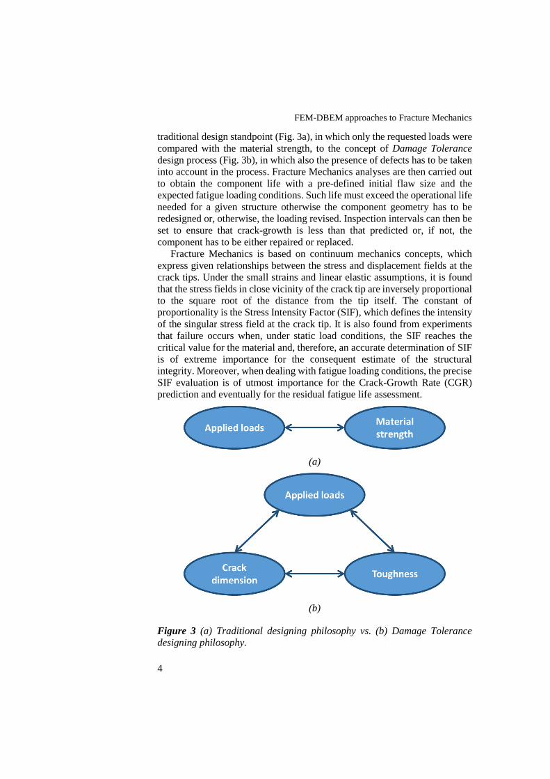
traditional design standpoint (Fig. 3a), in which only the requested loads were

compared with the material strength, to the concept of Damage Tolerance

design process (Fig. 3b), in which also the presence of defects has to be taken

into account in the process. Fracture Mechanics analyses are then carried out

to obtain the component life with a pre-defined initial flaw size and the

expected fatigue loading conditions. Such life must exceed the operational life

needed for a given structure otherwise the component geometry has to be

redesigned or, otherwise, the loading revised. Inspection intervals can then be

set to ensure that crack-growth is less than that predicted or, if not, the

component has to be either repaired or replaced.

Fracture Mechanics is based on continuum mechanics concepts, which

express given relationships between the stress and displacement fields at the

crack tips. Under the small strains and linear elastic assumptions, it is found

that the stress fields in close vicinity of the crack tip are inversely proportional

to the square root of the distance from the tip itself. The constant of

proportionality is the Stress Intensity Factor (SIF), which defines the intensity

of the singular stress field at the crack tip. It is also found from experiments

that failure occurs when, under static load conditions, the SIF reaches the

critical value for the material and, therefore, an accurate determination of SIF

is of extreme importance for the consequent estimate of the structural

integrity. Moreover, when dealing with fatigue loading conditions, the precise

SIF evaluation is of utmost importance for the Crack-Growth Rate (CGR)

prediction and eventually for the residual fatigue life assessment.

(a)

(b)

Figure 3 (a) Traditional designing philosophy vs. (b) Damage Tolerance

designing philosophy.

Chapter I

5

III Numerical analyses

Obviously, analytical techniques cannot tackle all the complexities

encountered in all the engineering structural components. Therefore,

numerical techniques have been widely developed in recent years, encouraged

especially by the enormous advances in the computer technology.

Nowadays, FEM is the most widely used in the engineering designing

process thanks to its advantages when simulating several physical phenomena.

The method is widely used in the industries since it is able to face problems

involving: contacts, frictions, mechanical, thermal and electromagnetical

loads, complex constitutive law formulations, impacts, etc. There are various

ways of tackling Fracture Mechanics by FEM and, definitely, FEM has been

efficiently used along the years in several applications. However, it typically

needs long model preparation times. In addition, especially when the crack

propagates generating complex three-dimensional shapes, the method is not

anymore suitable to simulate the fracture process due to distortion of elements

nearby the crack, too long runtimes, etc.

The Boundary Element Method, together with its enhanced version Dual

BEM, can circumvent the limitations of FEM on complex crack propagation

problems (Aliabadi, 1991, 1992; Brebbia, 1984, 1989). This method is based

on the solution of integral equations, that govern elasticity and potential

theory. Such a method works with the discretization of the only boundary into

elements over which the product of shape functions, Green’s functions and

element Jacobians, are numerically integrated. This results in higher accuracy

particularly when the domain to be discretised contains regions of high stress

gradients (such as cracks) which would necessitate a considerable

concentration of FEM elements and nodes. Hence, DBEM is particularly

suited to Fracture Mechanics analyses due to the accuracy of the results and

the inherently better and simpler remeshing process as the crack increases in

size.

Since only the boundaries of the domain are discretised, the dimensionality

of the domain is reduced by one, reducing then the size of the mathematical

problem to handle (Fig. 4). However, the system matrix is unsymmetric and

fully populated and therefore, generally, it takes longer runtimes than those

needed by FEM to obtain the solution. More generally, considering the

computational power nowadays available, DBEM remains more attractive,

when working on fracture, comparing the preprocessing efforts of the two

aforesaid numerical methods (Fig. 5).

FEM-DBEM approaches to Fracture Mechanics

6

(a) (b)

Figure 4 Example of a 2D model via (a) FEM and (b) BEM.

(a) (b)

Figure 5 Example of (a) FEM and (b) BEM models of a reinforced curved

fuselage panel (Aliabadi, 2002)

IV Boundary Element Method (BEM) and Dual BEM

BEM has become established as an effective alternative to FEM in several

important areas of engineering analysis. Although the BEM, also known as

the Boundary Integral Equation (BIE) method, is a relatively new technique

for engineering analysis the fundamentals can be traced back to classical

mathematical formulations by Fredholm (Fredholm, 1903) and Mikhlin

(Mikhlin, 1957) in potential theory and Betti (Betti, 1872), Somigliana

(Somigliana, 1886) and Kupradze (Kupradze, 1965) in elasticity.

Chapter I

7

Basically, the aim is to transform the governing differential equations

defined in the domain into an integral equation which applies only to the

boundary of the domain. Such an integral equation depends on the availability

of:

a fundamental solution to the governing differential equation for a

point force;

a reciprocal relationship (such as Green’s theorem; Green, 1828)

between two functions which are continuous and possess

continuous first derivatives.

The choice of the unknowns has led to two formulations of the boundary

integral equations: the direct method, where the unknowns are the actual

physical variables in the problem, such as displacement or traction in

elasticity; the indirect method that historically precedes the previous one. In

the latter approach, the unknowns are fictitious density functions which have

no physical significance but from which the physical unknowns can be

obtained by postprocess.

In order to obtain the boundary integral equations, a powerful and general

technique is the weighted residual method of Brebbia (1977, 1978) where the

error residual is minimized. Jeng and Wexler used a variational formulation

similar to that of the finite elements and Cruse and Rizzo (Rizzo, 1967; Cruse,

1969) employed Betti’s reciprocal work theorem.

For many years, the potential of boundary integral equations was not

realized due to the difficulty of attaining analytical solutions to the integral

equations for practical problems and due its essentially mathematical origins.

However, research into the numerical solution of boundary integral equations

was prompted by the advent of high speed computing. As computers grew in

power and storage, the amenable problems became more complex. This

resulted in the numerical method now known as BEM. Brebbia demonstrated

that not only it is related to FEM but that both methods can be derived from

the same variational equation (Brebbia, 1978).

In the BEM, the boundary integral equations are discretized so that

numerical integration is carried out over a small part (element) of the

boundary, over which the variation of the boundary variables is expected to

be small. Variation over an element is handled in a similar way to that of the

finite elements. For example, considering an elastostatic problem, the

variation of displacements and tractions over an element is approximated by

opportune shape functions related to nodal values of displacements and

tractions respectively. Each collocation node will yield either two or three

boundary integral equations depending on the dimensionality of the problem.

By moving this collocation point to each node in the model, a system of

equations is built up in which the displacement at each point is related to the

displacement and tractions on all points on the boundary. The resulting

matrices are therefore fully populated and unsymmetric. This is in contrast to

FEM-DBEM approaches to Fracture Mechanics

8

the sparse and banded FEM system matrix which, however, are generally

much larger for an equivalent problem.

It is worth noting that only the boundary of the model needs to be

discretized as the governing (elastostatic) differential equations are satisfied

in the interior region. The data preparation is carried out only for the boundary,

avoiding the domain discretization used by the FEM. This results in a method

that is particularly suited to Fracture Mechanics analyses due to the accuracy

of the results both on the surface and at selected interior points.

The introduction of isoparametric variation over the boundary elements by

Lachat and Lachat & Watson (Lachat, 1975, 1976) provided a further

possibility to the BEM to fulfil its potential of high accuracy and efficiency.

Quadratic variation of geometry was used over the elements and linear,

isoparametric quadratic and cubic variation of the unknown displacement and

traction were catered for. This enables the BEM to be more economical than

FEM for certain types of problems, although FEM will be more appropriate

for others. Anyway, both techniques should be made available to engineers.

The adopted DBEM approach (Portela, 1990, 1993; Apicella, 1994; Mi, 1994;

Fedelinsky, 1994) is a BEM enriched with special discontinuous elements

appropriate to consider nodes and faces of the crack topologically coincident.

The three-dimensional domain boundary is discretized into either 4, 8 or 9

noded quadrilateral elements, or 3 or 6 noded triangular elements. The

boundary integral equations here adopted apply to a homogeneous isotropic

domain and the linear elastic assumption must also be held. As aforesaid, with

DBEM, only the crack faces and the other boundaries are discretized. Traction

boundary integral equations are used for one crack face and displacement

boundary integral equations are used for the second crack face and the

remaining boundaries. So doing, being the traction and displacement

equations independent, the system coefficient matrix turns out to be non-

singular and, therefore, the solution can be retrieved.

V Description of Thesis

After an introduction, in chapter I it has been discussed on how to couple

the FEM and DBEM methods to work out general Fracture Mechanics

problems. At first, the need to adopt a submodelling strategy when solving

fracture problems on large structures has been introduced. Then, it has been

argued on how to implement such a submodelling technique by using the FEM

and DBEM methods. Three FEM-DBEM submodelling approaches have been

presented and the advantages of using the “Loaded Crack” (LC) approach

highlighted. By means of such an approach, based on loading only the DBEM

crack faces, the most accurate results in terms of SIFs, CGRs and crack paths

can be obtained.

Chapter I

9

In chapter II, it has been shown how the LC approach has been applied on

a shaft-hub coupling that undergoes different loading conditions. The results

have been compared with those obtained by leveraging on a pure DBEM

approach and with two different FEM codes showing a very sound agreement.

A first industrial application of the LC approach has been presented in

chapter III. It consisted in a crack propagation simulation in an airfoil of a

statoric segment of a GE-Aviation aeroengine. The LC approach turned out to

be more efficient in terms of computational effort and more accurate in terms

of fatigue life estimate, when compared with a classical FEM-DBEM

approach.

In chapter IV, it has been presented a further industrial application of the

three FEM-DBEM approaches on a component of the magnetic cage of the

nuclear fusion experiment “Wendelstein 7-X”. The residual fatigue life has

been estimated with all the approaches and the results compared and

discussed. Again, the LC approach turned out to be more accurate than the

classical approaches.

All the DBEM and FEM-DBEM calculations shown in chapters II-IV were

executed on a workstation with the following general configuration:

motherboard MSI X99S SLI Plus, CPU Intel i7-5820K with 15MB L3 cache,

RAM 8x 8GB HyperX Fury DDR4, SSD Samsung 850 2x 250GB and

Windows 7 Professional 64bit SP1.

At the end, final conclusions have been summarised.

Chapter I

FEM-DBEM approaches to

Fracture Mechanics

I.1 Introduction

FEM and BEM are effective tools for the numerical analysis of many

physical problems described with a set of partial differential equations and

frequently impossible to solve analytically.

With regard to particular aspects, the two methodologies are

complementary, each of them having preferential applications. Namely, FEM

is well suited for complex analyses containing nonlinearities, massive meshes,

contacts, anisotropic materials, etc., whereas BEM and in particular DBEM

(Dual BEM) (Aliabadi, 1992a, 1992b; Portela, 1990; Fedelinsky, 1994) are

generally preferred in the Linear Elastic Fracture Mechanics (LEFM) context,

to get accurate SIFs (Stress Intensity Factors) evaluations and automatic crack

propagations (Apicella, 1994).

Although the fracture phenomenon plays essentially a local effect if

compared to the overall structure (i.e. the singular fields at crack tip, the

possible crack propagation, etc.), it cannot be overlooked. An initial small

crack, after it propagates throughout the structure, can lead to the failure of

the entire structure as taught by well-known past catastrophic failures (Figs.

I.1, I.2). Numerical analysis can be used as a tool to better understand how

fracture phenomena affect structures in order to prevent catastrophic failures.

When one or more cracks have to be numerically modelled in large

structures, a submodelling approach is generally mandatory in order to make

the approach amenable from a computational standpoint and also to reduce

the size of the models to handle. Especially when such structures are modelled

by FEM, this submodelling approach plays an even more important role since

the cracks would need very fine meshes in their surroundings with the

consequent sharp increase of runtimes. The DBEM would be more attractive

in this context thanks to its intrinsic nature of meshing only the model

boundaries and one or multiple cracks can be modelled more easily than by

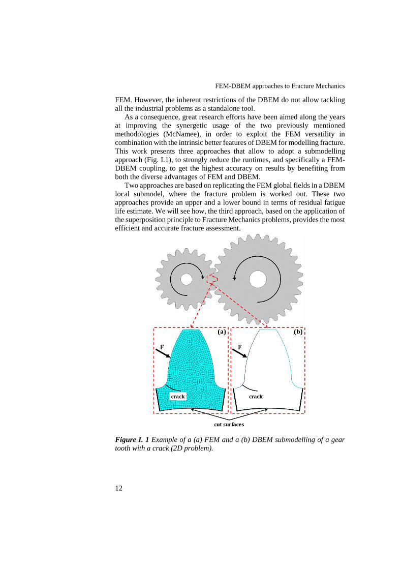
FEM-DBEM approaches to Fracture Mechanics

12

FEM. However, the inherent restrictions of the DBEM do not allow tackling

all the industrial problems as a standalone tool.

As a consequence, great research efforts have been aimed along the years

at improving the synergetic usage of the two previously mentioned

methodologies (McNamee), in order to exploit the FEM versatility in

combination with the intrinsic better features of DBEM for modelling fracture.

This work presents three approaches that allow to adopt a submodelling

approach (Fig. I.1), to strongly reduce the runtimes, and specifically a FEM-

DBEM coupling, to get the highest accuracy on results by benefiting from

both the diverse advantages of FEM and DBEM.

Two approaches are based on replicating the FEM global fields in a DBEM

local submodel, where the fracture problem is worked out. These two

approaches provide an upper and a lower bound in terms of residual fatigue

life estimate. We will see how, the third approach, based on the application of

the superposition principle to Fracture Mechanics problems, provides the most

efficient and accurate fracture assessment.

Figure I. 1 Example of a (a) FEM and a (b) DBEM submodelling of a gear

tooth with a crack (2D problem).

Chapter I

13

I.2 Superposition principle for Linear Elastic Fracture Mechanics

Wilson (Wilson, 1979) showed that the SIFs for a crack in a 2D thermal-

stress problem could be calculated by means of a simpler stress analysis in

which no external loads were applied but just tractions on the crack faces. This

was possible leveraging on the principle of linear superposition applied to a

Fracture Mechanics problem, as explained in the followings.

Figure I. 2 Superposition principle applied to a fracture problem; 𝜎0 is the

pre-existing stress field generated by the applied prescribed conditions, etc.

Extending the Wilson’s example to the most general crack problem

schematically shown in Fig. I.2, the superposition principle can be then

applied as explained in the following steps:

from an original uncracked domain (A), a crack can be opened (B)

and loaded with tractions equal to those calculated over the same

dashed line in (A);

the new configuration (B), perfectly equivalent to (A), can then be

transformed by using the superposition principle, splitting the

boundary conditions as in (C) and (D);

(C = C’) represents the real fracture problem to be solved, whereas

(D), after the tractions sign inversion, turns in an equivalent

problem (D’) that will be effectively tackled.

FEM-DBEM approaches to Fracture Mechanics

14

In conclusion, using boundary conditions retrieved from the considered

uncracked problem (A), a purely stress crack problem (D’) can be considered

for the fracture assessment; in such equivalent problem, the crack faces

undergo tractions equal in magnitude but opposite in sign to those calculated

over the same (dashed) crack line in (A). In other words, SIFs for case (C’)

are equal to those calculated for the simpler problem (D’). In final, the use of

the superposition principle enables a faster convergence for the simpler

DBEM pure stress analyses, in comparison with that provided by the more

traditional FEM-DBEM approaches (those with transfer of displacement or

traction boundary conditions on the submodel cut surfaces), with consequent

reduction of computational burden.

I.3 FEM-DBEM coupled approaches

Considering the different FEM and DBEM capabilities, the most

promising idea would be to use FEM to calculate the global displacement-

strain-stress fields and to adopt such results to solve the local fracture problem

by means of DBEM.

Here, two FEM-DBEM approaches are presented and, by considering the

superposition principle explained in §I.2, a third one is proposed. The three

approaches can be schematically explained by means of Fig. I.3. With

reference to cases (b) and (c) in Fig. I.3, all the rigid body degrees of freedom

have to be eliminated and this can done, as instance, by applying springs of

negligible stiffness on few elements.

Basically, all the approaches are based on the submodelling technique in

order to strongly reduce the computational efforts. The basic assumption is

that the analysed fracture phenomena do not introduce a significant

perturbation on the overall fields far from the crack area, so that, there is no

need to explicitly model the entire structure for the fracture assessment.

A DBEM submodel can be then extracted by a Boolean operation of

subtraction between the FEM model and a user defined cutting domain,

providing, in the DBEM environment, a smaller model that surrounds the

crack insertion area with just a surface mesh at its boundaries.

After the DBEM submodel extraction, a crack is inserted in the submodel

and a remeshing, which typically involves just the crack surroundings, is

realised. Subsequently, such DBEM cracked submodel is loaded with apposite

boundary conditions in order to compute SIFs representative of those

occurring in the real cracked component. Then, when requested, the crack

propagation can be simulated by increasing step-by-step the crack dimensions,

with the ith crack kinking and growth rate evaluated as a function of the SIFs

evaluated for the (i-1)th geometry. Moreover, for fatigue crack propagation

simulations, one or more load cases are used to assemble the needed fatigue

load spectra representative of the loads occurring during the real operation of

Chapter I

15

the components. Also, it has to be guaranteed that the crack tips remain

adequately far from the cut surface boundaries over which displacements or

traction were imposed.

Figure I. 3 Different approaches for the selection of the DBEM submodel

loading conditions for a gear tooth with a crack: (a) Fixed Displacement

(FD); (b) Fixed Load (FL); (c) Loaded Crack (LC).

The DBEM submodel loading process can follow one of the three different

previously mentioned approaches (example in Fig. I.3) explained in the

following:

Fixed Displacement (FD) approach: the DBEM volume cut

surfaces are loaded with displacement boundary conditions;

Fixed Load (FL) approach: the DBEM volume cut surfaces are

loaded with traction boundary conditions;

Loaded Crack (LC) approach: the DBEM crack faces are loaded

with traction boundary conditions.

In detail, two kind of inaccuracies unavoidably arise when using both FD

or FL approaches. Firstly, such two approaches use boundary conditions that

applied to a cracked model come from an uncracked global model. Secondly,

boundary conditions are kept as fixed during the crack propagation simulation

and therefore they are considered as insensitive to the continuously decreasing

DBEM submodel stiffness induced by the growing crack. Both inaccuracies

could be overcome by using a larger submodel but this would affect the

runtimes without even completely eliminate such drawbacks. Anyway, the FD

approach has been satisfactorily implemented in the past as in some works

available in the literature (Citarella, 2013, 2014).

On the contrary, the LC approach allows to inherently consider step-by-

step updated boundary conditions, since additional loading is provided on the

crack extension area at each step of the incremental crack-growth simulation.

In addition, the SIFs are rigorously calculated even by using boundary

conditions that are coming from an uncracked model, as dictated by the

superposition principle (§I.2). Moreover, there is no need to replicate the

global FEM fields in the DBEM submodel and this widen the range of

FEM-DBEM approaches to Fracture Mechanics

16

amenable applications, namely more complex analyses can be restricted solely

to FEM approach.

For these reasons, in the following it is shown that the LC approach

represents the most enhanced strategy to couple FEM and DBEM, providing

results with the highest accuracy in terms of SIF assessment and therefore also

in terms of residual fatigue life estimate and crack path assessment. Such an

approach is proposed in the current work by means of a FEM-DBEM

submodelling strategy but, however, it can clearly be also applicable to FEM-

FEM submodelling strategies or equivalents. It is worth noting that, for

embedded cracks far enough from the external boundaries (e.g. voids, internal

cracks), it would be possible to consider the cracks as in an infinite body so

the DBEM boundary would be just the loaded crack faces and the

corresponding mathematical problem notably reduced.

Besides the submodel loading conditions, in order to predict a Linear

Elastic Fracture Mechanics (LEFM) incremental crack-growth, three basic

criteria are required for the separate phases of: SIF evaluation, kink angle

prediction and Crack-Growth Rate (CGR) assessment. The criteria that have

been used in the current work are described in the followings together with

some references about the most widely accepted ones.

I.4 Crack-growth criteria

A crack-growth simulation is typically worked out by means of an

incremental crack-extension analysis in which the three distinct phases of SIF

evaluation, kink angle prediction and CGR assessment are basically repeated

until either a requested crack size or a critical K value is reached. Namely, for

each crack extension, the SIFs are calculated and used to predict both the

direction of the growth and the corresponding fatigue cycles. Various criteria

have been proposed along the years and those adopted in this work are

described in the followings.

I.4.1 SIF evaluation

There are several approaches to calculate SIFs such as: crack tip opening

displacement (CTOD) approach (Citarella, 2010), crack tip stress field

approach (Dhondt, 2014) and SIF extraction method from J-integral

(Citarella, 2010). The J-integral, being an energy approach, has the advantage

that elaborate representation of the crack tip singular fields is not necessary.

This is due to the relatively small contribution that the crack tip fields make

to the total J (i.e. strain energy) of the body. Therefore, in the present work,

the SIFs are extracted from the J-integral calculation by leveraging on the

method illustrated in the following.

Path independent J-integral is defined as:

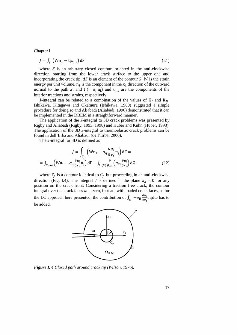
Chapter I

17

𝐽 = ∫ (Wn1 − tj𝑢j,1)𝑆

dS (I.1)

where 𝑆 is an arbitrary closed contour, oriented in the anti-clockwise

direction, starting from the lower crack surface to the upper one and

incorporating the crack tip, 𝑑𝑆 is an element of the contour 𝑆, 𝑊 is the strain

energy per unit volume, n1 is the component in the x1 direction of the outward

normal to the path 𝑆, and tj(= σijnj) and uj,1 are the components of the

interior tractions and strains, respectively.

J-integral can be related to a combination of the values of K𝐼 and K𝐼𝐼.

Ishikawa, Kitagawa and Okamura (Ishikawa, 1980) suggested a simple

procedure for doing so and Aliabadi (Aliabadi, 1990) demonstrated that it can

be implemented in the DBEM in a straightforward manner.

The application of the J-integral to 3D crack problems was presented by

Rigby and Aliabadi (Rigby, 1993, 1998) and Huber and Kuhn (Huber, 1993).

The application of the 3D J-integral to thermoelastic crack problems can be

found in dell’Erba and Aliabadi (dell’Erba, 2000).

The J-integral for 3D is defined as

𝐽 = ∫ (Wn1 − 𝜎ij

𝜕𝑢𝑖

𝜕𝑥1𝑛j) dΓ

Γ𝜌

=

= ∫ (Wn1 − 𝜎ij𝜕𝑢𝑖

𝜕𝑥1𝑛j) dΓ

𝐶+𝜔− ∫

𝜕

𝜕𝑥3(𝜎𝑖3

𝜕𝑢𝑖

𝜕𝑥1) dΩ

Ω(𝐶) (I.2)

where Γ𝜌 is a contour identical to C𝜌 but proceeding in an anti-clockwise

direction (Fig. I.4). The integral J is defined in the plane x3 = 0 for any

position on the crack front. Considering a traction free crack, the contour

integral over the crack faces 𝜔 is zero, instead, with loaded crack faces, as for

the LC approach here presented, the contribution of ∫ −𝜎ij𝜕𝑢𝑖

𝜕𝑥1𝑛jdω

𝜔 has to

be added.

Figure I. 4 Closed path around crack tip (Wilson, 1976).

FEM-DBEM approaches to Fracture Mechanics

18

For mixed-mode 3D problems, the J-integral is related to the three basic

fracture modes through the components JI, JII and JIII:

J = JI + JII + JIII (I.3)

Rigby and Aliabadi (Rigby, 1998) presented a decomposition method

through which the integrals JI, JII and JIII in elastic problems can be calculated

directly from J. Firstly, J was divided into two components:

J = JS + J𝐴𝑆 (I.4)

J𝑆 and JAS are obtained from symmetric and anti-symmetric elastic fields

around the crack plane, respectively. As the mode I elastic fields are

symmetric to the crack plane, the following relationship holds:

JS = J𝐼 and JAS = J𝐼𝐼 + J𝐼𝐼𝐼 (I.5)

JII and JIII integrals can be calculated from J𝐴𝑆 by making an additional

analysis on the anti-symmetric fields. Then, when J-integral is calculated as

sum of the three separated contributions of mode I, II and III, the Stress

Intensity Factors 𝐾i can be obtained as:

J = JI + JII + JIII =1

𝐸′(𝐾𝐼

2 + 𝐾𝐼𝐼2) +

1

2𝐺𝐾𝐼𝐼𝐼

2 (I.6)

where 𝐺 is the shear modulus and 𝐸′ = 𝐸 (Young’s modulus) for plane

stress, or 𝐸′ = 𝐸 (1 − 𝜈2)⁄ for plane strain.

The method for deriving the three separate K values from J can be found

in (Aliabadi, 2002) or (Rigby, 1998).

I.4.2 Kink angle assessment

Well-established criteria proposed for calculating the crack deflection

angles in isotropic media can be: Maximum Tangential Stress (MTS)

(Erdogan, 1963), Maximum Energy Release Rate (MERR) (Griffith, 1921,

1924), Minimum Strain Energy Density (MSED) (Sih, 1974), Maximum

Principal Asymptotic Stress (MPAS) field (Dhondt, 2001). The MSED

criterion has been adopted in the current work and some aspects about this

criterion are here provided.

MSED criterion is developed on the basis of the strain energy (𝑊) density

𝑑𝑊 𝑑𝑉⁄ concept (𝑑𝑉 is the differential volume). Fracture is assumed to

initiate from the nearest neighbour element located by a set of cylindrical

coordinates (𝑟, 𝜃, 𝜑) attached to the crack border. The new fracture surface is

described by a locus of these elements whose locations correspond to the strain

energy function being a minimum. The explicit expression of strain energy

density around the crack front tip can be written as:

𝑑𝑊

𝑑𝑉=

𝑆(𝜃)

𝑟 cos 𝜑+ 𝑂(1) (I.7)

Chapter I

19

where 𝑆(𝜃) is given by

𝑆(𝜃) = 𝑎11𝐾𝐼2 + 2𝑎12𝐾𝐼𝐾𝐼𝐼 + 𝑎22𝐾𝐼𝐼

2 + 𝑎33𝐾𝐼𝐼𝐼2 (I.8)

and

𝑎11 =1+cos 𝜃

16𝜋𝐺(3 − 4𝜈 − cos 𝜃) (I.9)

𝑎12 =sin 𝜃

8𝜋𝐺[cos 𝜃 − (1 − 2𝜈)] (I.10)

𝑎22 =1

16𝐺[4(1 − 𝜈)(1 − cos 𝜃) + (1 + cos 𝜃)(3 cos 𝜃 − 1)] (I.11)

𝑎33 =1

4𝜋𝐺 (I.12)

in which 𝐺 is the shear modulus of elasticity and 𝜈 is the Poisson ratio.

𝑆 rcos 𝜑⁄ represents the amplitude of the intensity of the strain energy density

field and it varies with the angle 𝜑 and 𝜃. It is apparent that the minimum of

𝑆 rcos 𝜑⁄ always occur in the normal plane of the crack front curve, namely

𝜑 = 0. 𝑆 is known as strain energy density factor and plays a similar role to

the SIF.

Such a criterion is based on three hypotheses:

1. the direction of the crack-growth at any point along the crack front

is toward the region with the minimum value of strain energy

density factor 𝑆 as compared with other regions on the same

spherical surface surrounding the point.

2. crack extension occurs when the strain energy density factor in the

region determined by hypothesis 𝑆 = 𝑆𝑚𝑖𝑛 reaches a critical value,

say 𝑆𝑐𝑟.

3. the length, 𝑟0, of the initial crack extension is assumed to be

proportional to 𝑆𝑚𝑖𝑛 such that 𝑆𝑚𝑖𝑛 𝑟0⁄ remains constant along the

new crack front.

It can be seen that the Minimum Strain Energy Density criterion can be

used both in two and three dimensions. Note that the direction evaluated by

the criterion in three-dimensional cases is insensitive to 𝐾𝐼𝐼𝐼 since the 𝑎33 does

not have a 𝜃 dependency (eq. I.12).

The crack-growth direction angle is obtained by minimising the strain

energy density factor 𝑆(𝜃) of eq. I.8 with respect to 𝜃. The minimum strain

energy density factor 𝑆𝑚𝑖𝑛 is then:

𝑑𝑆(𝜃)

𝑑𝜃= 0 − 𝜋 < 𝜃 < 𝜋 (I.13)

𝜃∗: {𝑚𝑖𝑛𝑆(𝜃)} = 𝑆𝑚𝑖𝑛 = 𝑆(𝜃∗) (I.14)

FEM-DBEM approaches to Fracture Mechanics

20

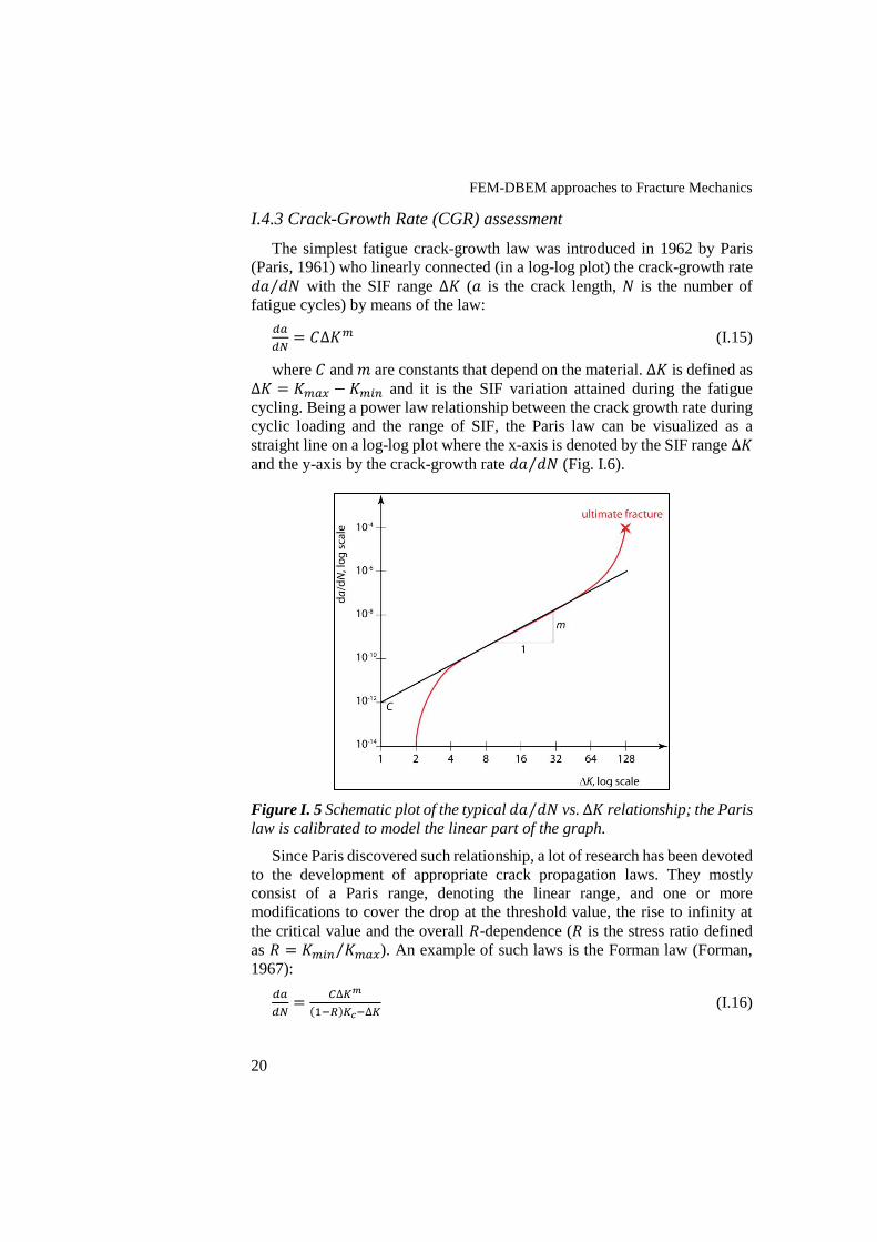
I.4.3 Crack-Growth Rate (CGR) assessment

The simplest fatigue crack-growth law was introduced in 1962 by Paris

(Paris, 1961) who linearly connected (in a log-log plot) the crack-growth rate

𝑑𝑎 𝑑𝑁⁄ with the SIF range ∆𝐾 (𝑎 is the crack length, 𝑁 is the number of

fatigue cycles) by means of the law:

𝑑𝑎

𝑑𝑁= 𝐶∆𝐾𝑚 (I.15)

where 𝐶 and 𝑚 are constants that depend on the material. ∆𝐾 is defined as

∆𝐾 = 𝐾𝑚𝑎𝑥 − 𝐾𝑚𝑖𝑛 and it is the SIF variation attained during the fatigue

cycling. Being a power law relationship between the crack growth rate during

cyclic loading and the range of SIF, the Paris law can be visualized as a

straight line on a log-log plot where the x-axis is denoted by the SIF range ∆𝐾

and the y-axis by the crack-growth rate 𝑑𝑎 𝑑𝑁⁄ (Fig. I.6).

Figure I. 5 Schematic plot of the typical 𝑑𝑎 𝑑𝑁⁄ vs. ∆𝐾 relationship; the Paris

law is calibrated to model the linear part of the graph.

Since Paris discovered such relationship, a lot of research has been devoted

to the development of appropriate crack propagation laws. They mostly

consist of a Paris range, denoting the linear range, and one or more

modifications to cover the drop at the threshold value, the rise to infinity at

the critical value and the overall 𝑅-dependence (𝑅 is the stress ratio defined

as 𝑅 = 𝐾𝑚𝑖𝑛 𝐾𝑚𝑎𝑥⁄ ). An example of such laws is the Forman law (Forman,

1967):

𝑑𝑎

𝑑𝑁=

𝐶∆𝐾𝑚

(1−𝑅)𝐾𝑐−∆𝐾 (I.16)

Chapter I

21

where 𝐾𝑐 is a further material parameter representative of the critical value

of 𝐾 that leads to the final fracture. A further example is the Walker law

(Walker, 1970) that takes into account of the R-dependence in the form of:

𝑑𝑎

𝑑𝑁= 𝐶 [

∆𝐾

(1−𝑅)1−𝑤]𝑚

(I.17)

with 𝑤 as a material parameter that defines the material sensibility to the

mean stress. The most complete crack-growth law is the NASGRO law

(NASGRO®, 2002) defined as:

𝑑𝑎

𝑑𝑁= 𝐶 (

(1−𝑓)

(1−𝑅)∆𝐾)

𝑚 (1−∆𝐾𝑡ℎ

∆𝐾)

𝑝

(1−𝐾𝑚𝑎𝑥

𝐾𝑐)

𝑞 (I.18)

where the number of material parameters needed to calibrate the law rises

up to 8. Further details can be found in (NASGRO®, 2002), however, the law

takes into account of the dependencies on the stress ratio 𝑅, 𝐾𝑡ℎ threshold

value, critical 𝐾𝑐 value and small crack propagation phenomenon.

Further crack-growth laws have been proposed in the literature (Dhondt,

2015).

I.4.4 Mixed-mode crack-growth

All the crack-growth laws defined in §I.4.3 are functions of the variability

of SIFs ∆𝐾 during the fatigue cycling. However, as described in §I.4.1, three

separate 𝐾 values (𝐾𝐼 , 𝐾𝐼𝐼 , 𝐾𝐼𝐼𝐼), representative of the three basic fracture

modes, are generally obtained by the J-integral decomposition. Therefore, it

is necessary to blend together the three distinct 𝐾 values in one single

“equivalent” 𝐾𝑒𝑞 value to use in a CGR law, this especially when all the three

𝐾 values are non-negligible (mixed-mode conditions). Some equations to

calculate 𝐾𝑒𝑞 from (𝐾𝐼 , 𝐾𝐼𝐼 , 𝐾𝐼𝐼𝐼), calibrated on experimental data, are

available in the literature and the most relevant ones are here presented:

Yaoming-Mi (Mi, 1995) formula:

𝐾𝑒𝑞 = √(𝐾𝐼 + |𝐾𝐼𝐼𝐼|)2 + 2𝐾𝐼𝐼2 (I.19)

Sum of squares (Beasy, 2011) formula:

𝐾𝑒𝑞 = √𝐾𝐼2 + 𝐾𝐼𝐼

2 + 𝐾𝐼𝐼𝐼2 (I.20)

Tanaka (Tanaka, 1974) formula:

𝐾𝑒𝑞 = √𝐾𝐼4 + 8𝐾𝐼𝐼

4 +8

1−𝜈𝐾𝐼𝐼𝐼

44 (I.21)

Chapter II

FEM-DBEM benchmark

II.1 Introduction

The work presented in this chapter is based on a benchmarking activity

between different numerical approaches to solve a fracture problem. Two

FEM codes, ZENCRACK (Zencrack, 2005) and CRACKTRACER3D

(Bremberg, 2008, 2009), a DBEM code (BEASY, 2011) and a FEM-DBEM

coupled approach have been separately used to calculate Stress Intensity

Factors (SIFs), Crack Growth Rates (CGRs) and crack paths for a crack

initiated from the outer surface of a shaft undergoing different load cases. The

main goal was to get a cross comparison on the results obtained by means of

different codes and eventually validate the coupled FEM-DBEM “Loaded

Crack” (LC) approach. The comparison was carried out in terms of the so

obtained SIFs, kink angles and CGRs and the result are here compared and

discussed showing a mutual agreement. Further details can be found in the

literature (Citarella, 2017; Giannella, 2017b).

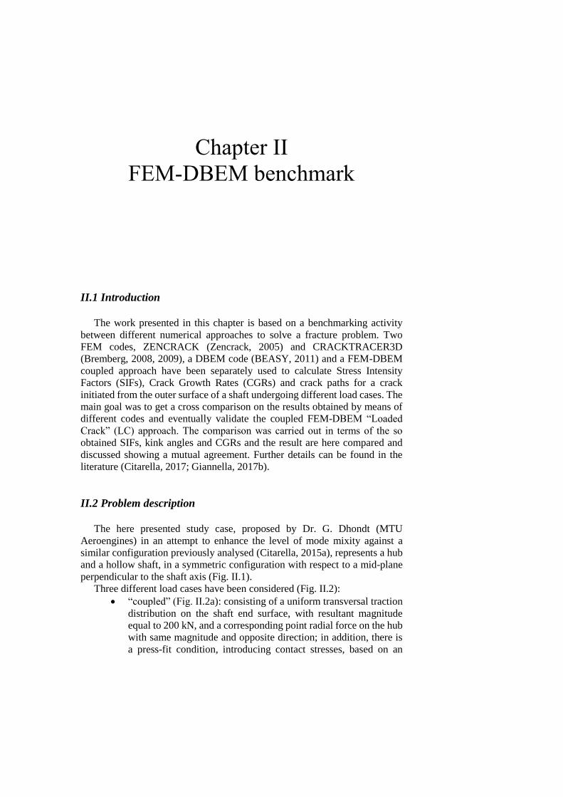
II.2 Problem description

The here presented study case, proposed by Dr. G. Dhondt (MTU

Aeroengines) in an attempt to enhance the level of mode mixity against a

similar configuration previously analysed (Citarella, 2015a), represents a hub

and a hollow shaft, in a symmetric configuration with respect to a mid-plane

perpendicular to the shaft axis (Fig. II.1).

Three different load cases have been considered (Fig. II.2):

“coupled” (Fig. II.2a): consisting of a uniform transversal traction

distribution on the shaft end surface, with resultant magnitude

equal to 200 kN, and a corresponding point radial force on the hub

with same magnitude and opposite direction; in addition, there is

a press-fit condition, introducing contact stresses, based on an

FEM-DBEM benchmark

24

interference 𝛿 = 0.28 𝑚𝑚 at shaft/hub contact surface with a

static friction coefficient 𝑓𝑠 = 0.6;

“shear” (Fig. II.2b): consisting of a uniform transversal force

distribution, with resultant magnitude equal to 200 kN, along the

hub perimeter line (dotted red line of Fig. II.1b);

“torque” (Fig. II.2c): consisting of a uniform torque distribution,

with resultant magnitude equal to 22.5 kN m, again distributed

along the hub perimeter line (dotted red line of Fig. II.1b).

(a)

(b)

Figure II. 1 Drawings of the (a) shaft with highlight of the crack and fillet

radii, (b) hub with the dotted red line representing the loading application

zone.

Chapter II

25

(a)

(b)

(c)

Figure II. 2 Considered load cases: (a) ‘‘coupled”, (b) ‘‘shear” and (c)

‘‘torque”.

The material is a steel, whose behaviour is assumed being linear-elastic,

with the main mechanical and fracture material data listed in Tab. II.1. The

geometry of the initially considered part-through crack is an arch of ellipse;

the crack is initiated from the external surface of the shaft, having dimensions

of 𝑎 = 3.8 𝑚𝑚 and 𝑐 = 1.9 𝑚𝑚 (Fig. II.1a).

Four different numerical approaches have been compared to simulate the

crack propagation:

“BEASY” DBEM code: the modelling, the propagation and the

stress calculations are performed within the DBEM environment;

“ZENCRACK” FEM code (hereinafter “ZC”): the stress

calculations are performed by the FEM‐ solver ABAQUS

FEM-DBEM benchmark

26

(ABAQUS, 2011), and both the modelling and the propagation are

performed within ZC;

“CRACKTRACER3D” FEM code (hereinafter “CT3D”):

CalculiX (Dhondt, 2016) is used as FE solver whereas the fracture

problem is left to CT3D;

“Loaded Crack” approach (hereinafter “LC”): a FEM code

(ABAQUS, 2011) is used to compute the global stress field in the

uncracked domain and such results are used to perform the DBEM

(BEASY, 2011) fracture analysis on the cracked subdomain (§I.3).

The adopted propagation law is a pure Paris‐ type (no threshold nor critical

value, §I.4.3). The needed Stress Intensity Factors (SIFs) were calculated by

using the J‐ integral approach in BEASY (Rigby, 1993, 1998) and ZC,

whereas in CT3D, the crack tip stress method was applied (Dhondt, 2001).

Because some of the loadings were truly mixed‐ mode (especially the

torque load case; Marcon, 2014; Berto, 2013; Citarella, 2015b), predictive

capabilities for out‐ of‐ plane crack-growth were particularly important for

this analyses. To this end, the propagation angle predictions were based on:

Minimum Strain Energy Density criterion (MSED; Sih, 1974) in BEASY,

Maximum Energy Release Rate (MERR) in ZC and, finally, the maximum

principal asymptotic stress criterion (Dhondt, 2014) in CT3D.

Table II. 1 Main material data for mechanical and fracture analyses.

Parameter Value

E [GPa] 210

ν [-] 0.3

C [mm/cycle/(MPa mm)0.5)n] 1.23085E-12

m [-] 2.8

ΔKth [(MPa mm)0.5] 0

Kc [(MPa mm)0.5] 1E6

II.3 DBEM modelling

The DBEM model is made up of two different zones (one for the shaft and

one for the hub), with a mesh of quadrilateral 9-noded boundary elements for

both functional and geometrical variables.

A part‐ through crack was inserted on the shaft external surface, see Fig.

II.3. After the crack insertion (fully automatic together with the inherent local

remeshing with 6 noded triangular boundary elements), the number of

elements increased from 2500 to nearly 3100.

Chapter II

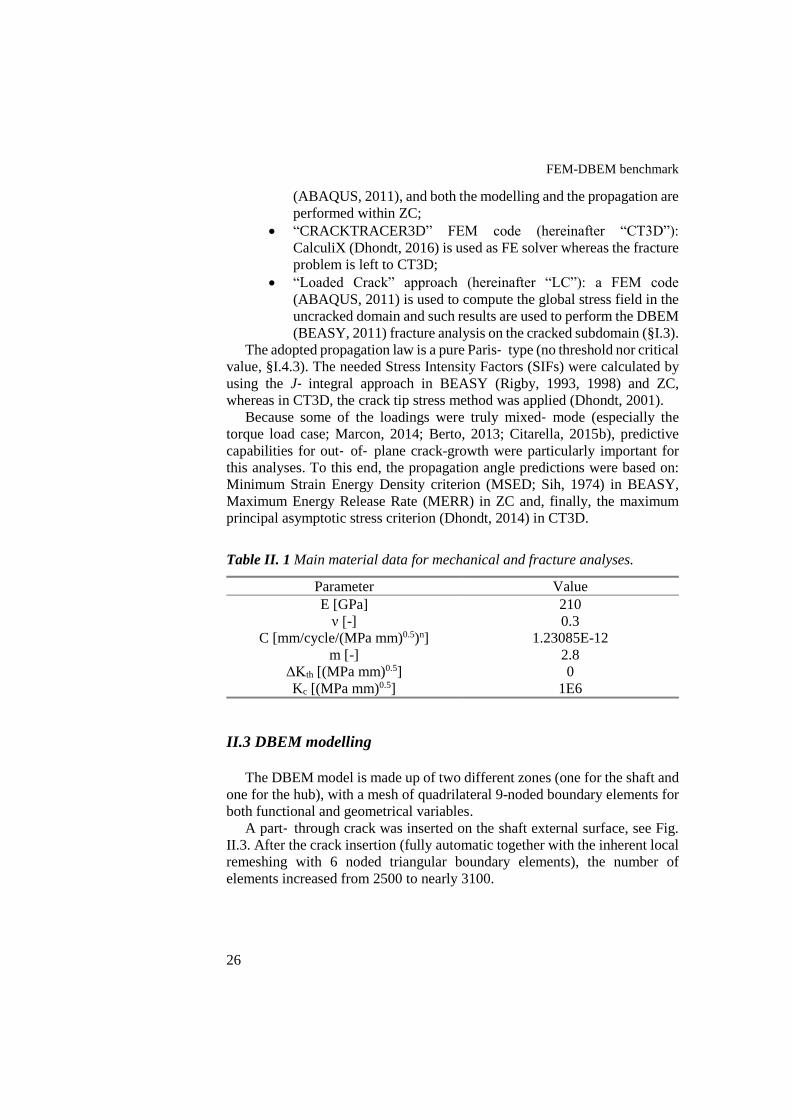
27

Figure II. 3 DBEM uncracked model with close‐ up of the remeshed area

surrounding the crack insertion point and details of the initial crack geometry

with J‐ paths along the crack front (purple) for the J‐ integral computation.

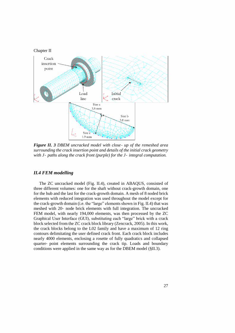
II.4 FEM modelling

The ZC uncracked model (Fig. II.4), created in ABAQUS, consisted of

three different volumes: one for the shaft without crack-growth domain, one

for the hub and the last for the crack-growth domain. A mesh of 8 noded brick

elements with reduced integration was used throughout the model except for

the crack-growth domain (i.e. the “large” elements shown in Fig. II.4) that was

meshed with 20‐ node brick elements with full integration. The uncracked

FEM model, with nearly 194,000 elements, was then processed by the ZC

Graphical User Interface (GUI), substituting each “large” brick with a crack

block selected from the ZC crack block library (Zencrack, 2005). In this work,

the crack blocks belong to the L02 family and have a maximum of 12 ring

contours delimitating the user defined crack front. Each crack block includes

nearly 4000 elements, enclosing a rosette of fully quadratics and collapsed

quarter‐ point elements surrounding the crack tip. Loads and boundary

conditions were applied in the same way as for the DBEM model (§II.3).

FEM-DBEM benchmark

28

Figure II. 4 ZENCRACK (ZC)/ABAQUS uncracked model with highlight on

the brick elements that are subsequently substituted with crack blocks.

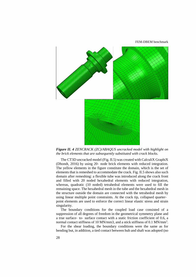
The CT3D uncracked model (Fig. II.5) was created with CalculiX GraphiX

(Dhondt, 2016) by using 20‐ node brick elements with reduced integration.

The yellow elements in the figure constitute the domain, which is the set of

elements that is remeshed to accommodate the crack. Fig. II.5 shows also such

domain after remeshing: a flexible tube was introduced along the crack front

and filled with 20 noded hexahedral elements with reduced integration,

whereas, quadratic (10 noded) tetrahedral elements were used to fill the

remaining space. The hexahedral mesh in the tube and the hexahedral mesh in

the structure outside the domain are connected with the tetrahedral mesh by

using linear multiple point constraints. At the crack tip, collapsed quarter‐point elements are used to enforce the correct linear elastic stress and strain

singularity.

The boundary conditions for the coupled load case consisted of a

suppression of all degrees of freedom in the geometrical symmetry plane and

a true surface‐ to‐ surface contact with a static friction coefficient of 0.6, a

normal contact stiffness of 10 MN/mm3, and a stick stiffness of 0.1 MN/mm3.

For the shear loading, the boundary conditions were the same as for

bending but, in addition, a tied contact between hub and shaft was adopted (no

Chapter II

29

relative motion possible between shaft and hub). Finally, for the torsion

loading, the displacements in axial and circumferential directions in the

geometrical symmetry plane were set to 0 and tied contact was applied

between the shaft and the hub.

Figure II. 5 CRACKTRACER3D (CT3D)/CalculiX uncracked model with the

subsequent cracked mesh and details of the crack.

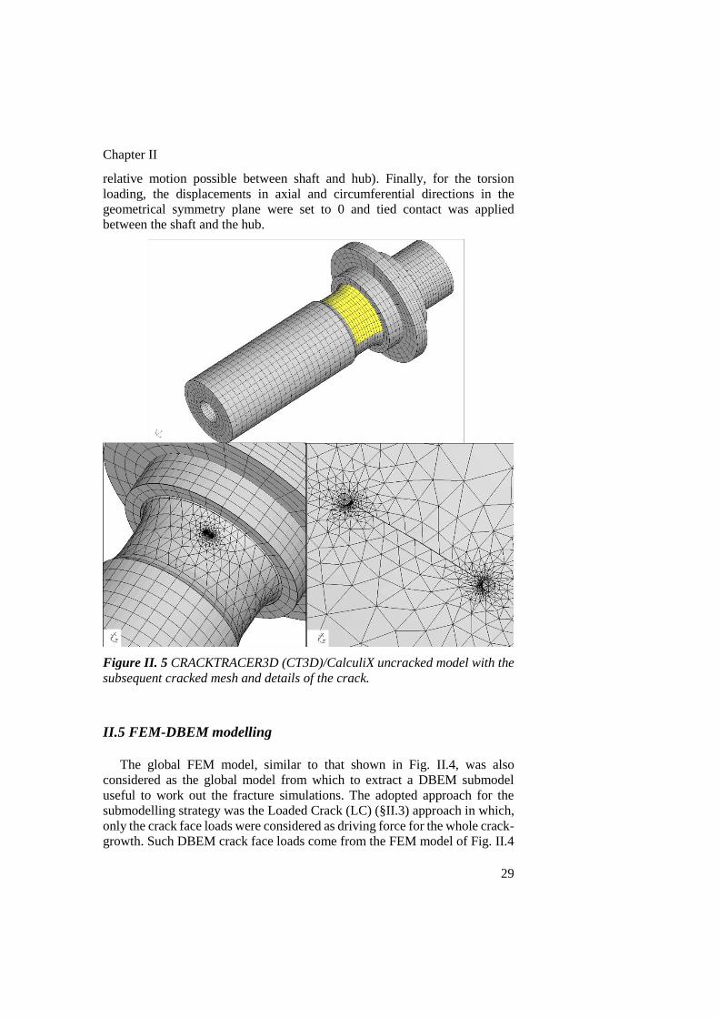
II.5 FEM-DBEM modelling

The global FEM model, similar to that shown in Fig. II.4, was also

considered as the global model from which to extract a DBEM submodel

useful to work out the fracture simulations. The adopted approach for the

submodelling strategy was the Loaded Crack (LC) (§II.3) approach in which,

only the crack face loads were considered as driving force for the whole crack-

growth. Such DBEM crack face loads come from the FEM model of Fig. II.4

FEM-DBEM benchmark

30

in which, the large crack elements were substituted with a fine mesh. In

particular, the stresses along the virtual surface traced by the crack have to be

evaluated with the highest possible precision, because they represent the

driving force for the following DBEM crack propagation.

When using such an LC approach, the FEM mesh in the cracked area has

to be very fine to retrieve accurate tractions to be applied on the DBEM crack

faces. For this reason, a FEM submodel (Fig. II.6a), containing a small portion

of the shaft, was extracted from the FEM global model to accurately calculate

the local stress field. Such submodel, containing only the volume surrounding

the crack insertion point, has size and mesh refinement capable to guarantee a

very high accuracy when evaluating the stress field in the neighbourhood of

the crack (higher than that provided by the global model). To get the needed

precision, especially for the torque load case, it has been necessary to strongly

refine the FEM submodel mesh. This was due to the high kink angles predicted

for the torque load case (nearly 90° for the initial propagation steps) that

required small crack advances per step and consequent heavy DBEM mesh

refinements.

Subsequently, a BEM submodel (Fig. II.6a) is created containing the zone

surrounding the crack initiation point (the crack is not yet modelled and that

is why the DBEM formulation is not yet enforced). In addition to the FEM

stresses, applied as tractions on the crack faces (Fig. II.6b), springs of

negligible stiffness (in purple in Fig. II.6a) are applied to a few BEM elements

in order to prevent rigid body motion (nodal rigid body constraints are

prevented in case of crack propagation). Due to the loading conditions

consisting of just a self-equilibrated load, a large part of the DBEM cracked

submodel (now the crack has been introduced with automatic remeshing in

the surrounding area) turns out to have a null stress field. For this reason, the

fracture problem can be analysed considering a very small portion of the entire

model, with inherent decrease of the needed computational effort.

Chapter II

31

(a)

(b)

Figure II. 6 (a) FEM and DBEM submodel used for the FEM-DBEM

approach; (b) DBEM submodel after that the crack has been inserted and

loaded.

The FEM submodel of Fig. II.6a, when used for the coupled and shear load

cases, comprised nearly 25,000 hexahedral elements whereas, for the torque

load case, comprised nearly 130,000 hexahedral elements.

A preliminary study was aimed at assessing the minimum needed

dimensions of the DBEM submodel, useful to guarantee a complete vanishing

of stresses from the crack area to the boundaries. Such uncracked DBEM

model comprises nearly 1200 linear elements and this number rises up to

nearly 1800 when the initial crack is inserted. The remeshing zone and the

crack faces are discretised with 9 noded quadratic elements whereas 4 noded

linear elements are used for the bulk of the remaining mesh.

II.6 Results

A crack-growth was simulated for each of the four abovementioned

approaches in correspondence of three loading conditions. Results are here

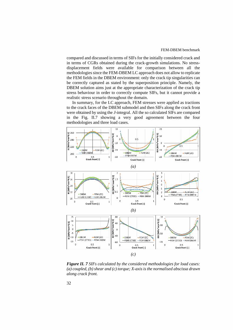
FEM-DBEM benchmark

32

compared and discussed in terms of SIFs for the initially considered crack and

in terms of CGRs obtained during the crack-growth simulations. No stress-

displacement fields were available for comparison between all the

methodologies since the FEM-DBEM LC approach does not allow to replicate

the FEM fields in the DBEM environment: only the crack tip singularities can

be correctly captured as stated by the superposition principle. Namely, the

DBEM solution aims just at the appropriate characterization of the crack tip

stress behaviour in order to correctly compute SIFs, but it cannot provide a

realistic stress scenario throughout the domain.

In summary, for the LC approach, FEM stresses were applied as tractions

to the crack faces of the DBEM submodel and then SIFs along the crack front

were obtained by using the J-integral. All the so calculated SIFs are compared

in the Fig. II.7 showing a very good agreement between the four

methodologies and three load cases.

(a)

(b)

(c)

Figure II. 7 SIFs calculated by the considered methodologies for load cases:

(a) coupled, (b) shear and (c) torque; X-axis is the normalised abscissa drawn

along crack front.

Chapter II

33

Crack propagation simulations were run considering a 0-max fatigue load

cycle with the maximum value corresponding to the loads defined in §II.2.

The simulations were all performed through a step-by-step growth of the

crack, involving a remeshing and a stress field evaluation (with corresponding

SIFs) at each crack-growth increment. The codes used in this work calculate

the kink angles in different ways: MSED by BEASY, MERR by ZC, and

maximum principal asymptotic stress criterion by CT3D.

A pure Paris’ law (§I.4.4; Paris, 1961) was adopted to predict the Crack

Propagation Rates for all the codes:

da

𝑑𝑁= 𝐶∆𝐾𝑒𝑞

𝑚 (II.1)

where the material parameters 𝐶 and 𝑚 are listed in Tab. II.1. ∆𝐾𝑒𝑞 is an

equivalent SIF, calculated by different combinations of mode I, II, and III

SIFs, depending on the considered code.

In particular, for the DBEM and FEM-DBEM approaches here adopted,

the procedure based on the decomposition of the elastic field into respective

symmetric and antisymmetric mode components, available in §I.4.1 (Rigby,

1993, 1998), was adopted to obtain the three separate 𝐾𝐼, 𝐾𝐼𝐼 and 𝐾𝐼𝐼𝐼 values.

Then, the ∆𝐾𝑒𝑞, in case of 𝑅 = 0, can be obtained by means of the Tanaka

formula (§II.4.4) here reported:

𝐾𝑒𝑞 = √𝐾𝐼4+8𝐾𝐼𝐼

4+8

1−𝜈𝐾𝐼𝐼𝐼

44 (I.19)

Regarding the ZC code, the total energy release rate was used for

calculating the 𝐾𝑒𝑞:

𝐾𝑒𝑞 = √[𝐸

1−(𝛼𝜈)2 𝐺𝑒𝑓𝑓], (II.2)

where α is a measure for the stress state taking values between 0 and 1 (0

for plane stress state and for plane strain state) whereas 𝐺𝑒𝑓𝑓, in case of 𝑅 =

0, corresponds to:

𝐺𝑒𝑓𝑓 =𝐵

𝐸(𝐾𝐼

2 + 𝐾𝐼𝐼2) +

1

2𝐺𝐾𝐼𝐼𝐼

2 , (II.3)

where 𝐵 = 1 − 𝜈2 for plane strain and 𝐵 = 1 for plane stress, and 𝐺 is the

shear modulus.

Finally, the calculation of the equivalent SIF is more cumbersome in the

CT3D code. Using the K‐ values of the three modes, the asymptotic stress

field is considered at each position along the crack front; the 𝐾𝑒𝑞 is then

defined as the principal self‐ similar stress evaluated in correspondence of the

deflection angle φ for which the principal plane contains the crack tip. The

corresponding principal plane dictates also the propagation direction. For any

details, the reader is referred to the paper by Dhondt (Dhondt, 2014).

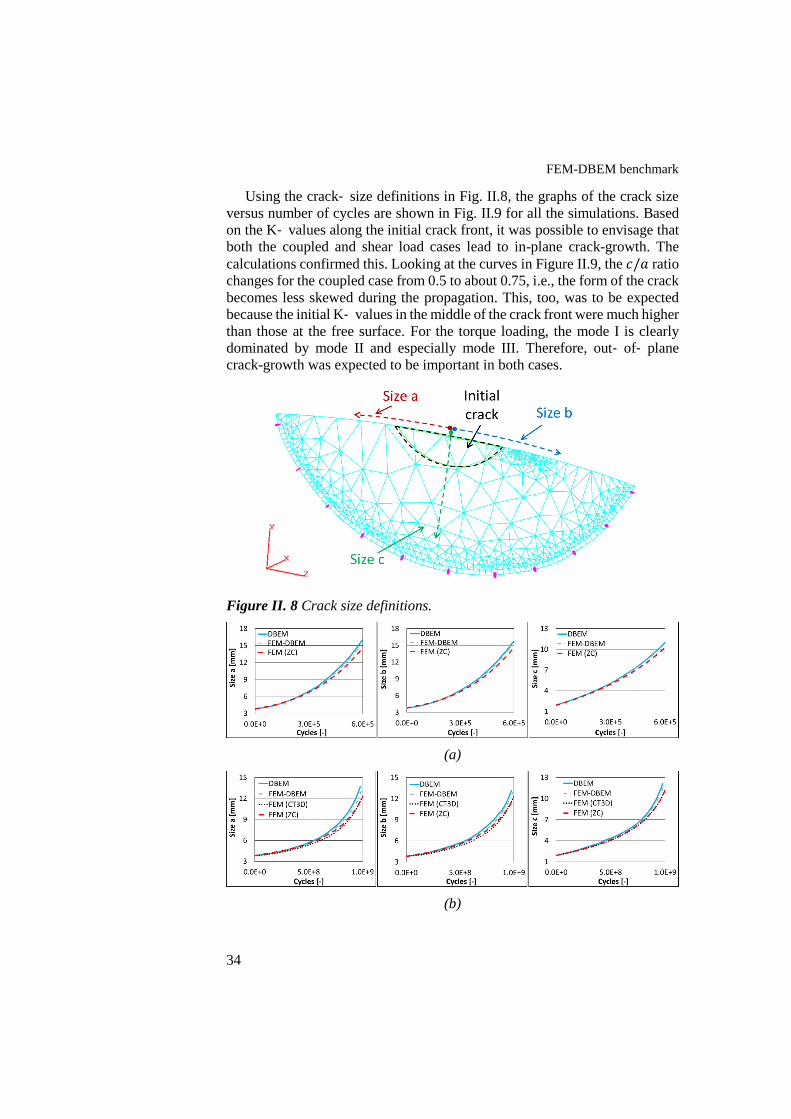
FEM-DBEM benchmark

34

Using the crack‐ size definitions in Fig. II.8, the graphs of the crack size

versus number of cycles are shown in Fig. II.9 for all the simulations. Based

on the K‐ values along the initial crack front, it was possible to envisage that

both the coupled and shear load cases lead to in-plane crack-growth. The

calculations confirmed this. Looking at the curves in Figure II.9, the 𝑐/𝑎 ratio

changes for the coupled case from 0.5 to about 0.75, i.e., the form of the crack

becomes less skewed during the propagation. This, too, was to be expected

because the initial K‐ values in the middle of the crack front were much higher

than those at the free surface. For the torque loading, the mode I is clearly

dominated by mode II and especially mode III. Therefore, out‐ of‐ plane

crack-growth was expected to be important in both cases.

Figure II. 8 Crack size definitions.

(a)

(b)

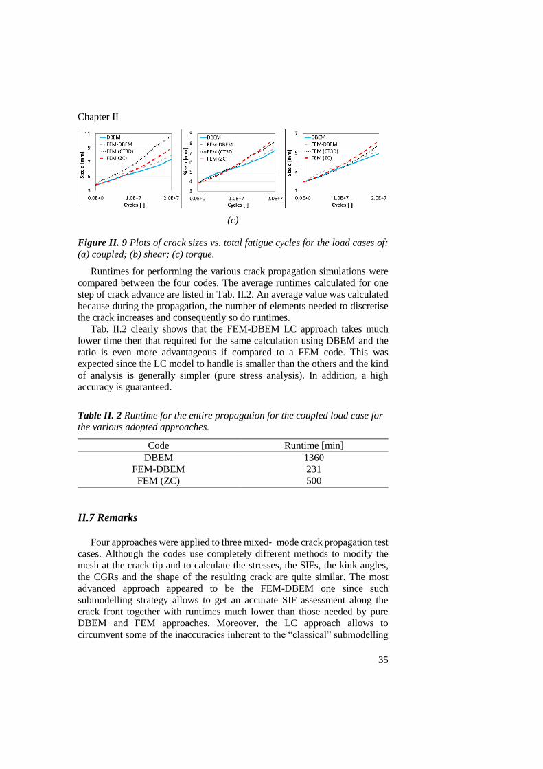
Chapter II

35

(c)

Figure II. 9 Plots of crack sizes vs. total fatigue cycles for the load cases of:

(a) coupled; (b) shear; (c) torque.

Runtimes for performing the various crack propagation simulations were

compared between the four codes. The average runtimes calculated for one

step of crack advance are listed in Tab. II.2. An average value was calculated

because during the propagation, the number of elements needed to discretise

the crack increases and consequently so do runtimes.

Tab. II.2 clearly shows that the FEM-DBEM LC approach takes much

lower time then that required for the same calculation using DBEM and the

ratio is even more advantageous if compared to a FEM code. This was

expected since the LC model to handle is smaller than the others and the kind

of analysis is generally simpler (pure stress analysis). In addition, a high

accuracy is guaranteed.

Table II. 2 Runtime for the entire propagation for the coupled load case for

the various adopted approaches.

Code Runtime [min]

DBEM 1360

FEM-DBEM 231

FEM (ZC) 500

II.7 Remarks

Four approaches were applied to three mixed‐ mode crack propagation test

cases. Although the codes use completely different methods to modify the

mesh at the crack tip and to calculate the stresses, the SIFs, the kink angles,

the CGRs and the shape of the resulting crack are quite similar. The most

advanced approach appeared to be the FEM-DBEM one since such

submodelling strategy allows to get an accurate SIF assessment along the

crack front together with runtimes much lower than those needed by pure

DBEM and FEM approaches. Moreover, the LC approach allows to

circumvent some of the inaccuracies inherent to the “classical” submodelling

FEM-DBEM benchmark

36

implementations. One of the reasons is that, with the LC approach, the loads

on the submodel (namely on the crack faces), are rigorously updated for each

step of the incremental crack-growth.

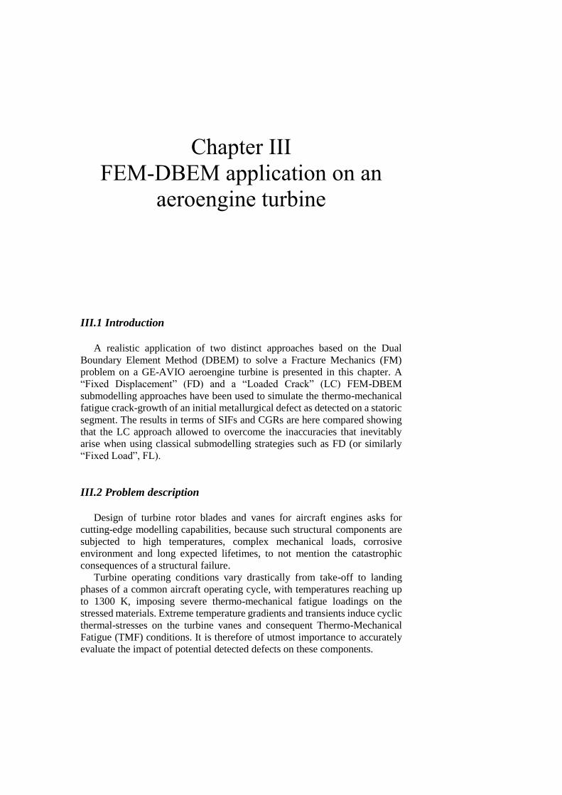
Chapter III

FEM-DBEM application on an

aeroengine turbine

III.1 Introduction

A realistic application of two distinct approaches based on the Dual

Boundary Element Method (DBEM) to solve a Fracture Mechanics (FM)

problem on a GE-AVIO aeroengine turbine is presented in this chapter. A

“Fixed Displacement” (FD) and a “Loaded Crack” (LC) FEM-DBEM

submodelling approaches have been used to simulate the thermo-mechanical

fatigue crack-growth of an initial metallurgical defect as detected on a statoric

segment. The results in terms of SIFs and CGRs are here compared showing

that the LC approach allowed to overcome the inaccuracies that inevitably

arise when using classical submodelling strategies such as FD (or similarly

“Fixed Load”, FL).

III.2 Problem description

Design of turbine rotor blades and vanes for aircraft engines asks for

cutting-edge modelling capabilities, because such structural components are

subjected to high temperatures, complex mechanical loads, corrosive

environment and long expected lifetimes, to not mention the catastrophic

consequences of a structural failure.

Turbine operating conditions vary drastically from take-off to landing

phases of a common aircraft operating cycle, with temperatures reaching up

to 1300 K, imposing severe thermo-mechanical fatigue loadings on the

stressed materials. Extreme temperature gradients and transients induce cyclic

thermal-stresses on the turbine vanes and consequent Thermo-Mechanical

Fatigue (TMF) conditions. It is therefore of utmost importance to accurately

evaluate the impact of potential detected defects on these components.

Aeroengine turbine FEM-DBEM application

38

To this aim, two FEM-DBEM submodelling strategies have been adopted

in this work to solve a realistic fracture problem in an aircraft engine turbine

stage. As proved in recent works, FEM and DBEM methods can efficiently

work together when tackling large structures (Citarella, 2013, 2014), residual

stresses generated by plastic deformations (Citarella, 2014, 2016a, 2016c;

Carlone, 2015) or load spectrum effects (Citarella, 2009).

The two procedures are tested on the crack scenario detected on a turbine

vane of a commercial aircraft engine. The load spectrum driving the fatigue

crack propagation is representative of a GAG (ground-air-ground) cycle. The

range of Stress Intensity Factors (∆𝐾) is used as the crack driving force and

Crack Growth Rates (CGRs) are calculated by using a Paris’ law (§I.4.3; Paris,

1961) calibrated by material fatigue crack-growth data obtained at the

temperature of interest.

The FEM and DBEM used codes are ANSYS (ANSYS, 2007) and BEASY

(BEASY, 2011) respectively.

III.3 FEM modelling

The global FEM model considered in the analyses is representative of a

statoric segment, made of six airfoils, of a low pressure turbine stage of a

commercial aircraft engine. It was modelled considering a typical turbine

blade superalloy, with mechanical and thermal isotropic material properties,

whose variations against temperature are illustrated in Fig. III.1. Fluid

pressure was modelled as a mechanical load, applied on both sides of the

airfoils, in addition to the temperature scenario, previously calculated by

thermo-fluid-dynamic analyses (Fig. III.2a). In addition, cyclic symmetry

boundary conditions were enforced on the casing that couples with the statoric

segment, in order to simulate the circumferential periodicity of the entire stage

(Fig. III.2b). Surface to surface contacts were applied on the interfaces

between statoric hooks and casing. Thermal and mechanical loads applied on

the global model were representative of the most severe conditions for an

aircraft engine during its mission, namely, those reached at take-off. As a

matter of fact, during the take-off, there is the need for the maximum boost of

the engines and, consequently, vane temperatures get the highest magnitudes

and the highest gradients with consequent enhancement of the so generated

thermal-stresses.

In correspondence of the boundary conditions related to the most critical

mission point, a tangential displacement distribution was evaluated (Fig.

III.3a). Due to a combination of mechanical and thermal cyclic stresses,

fatigue cracks can nucleate, most likely from locations with highest stresses,

localized in-between airfoils and casing (Fig. III.3b, the figure shows also the

crack insertion point for the subsequent fracture analyses).

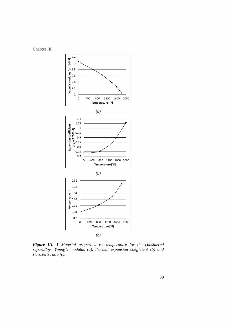
Chapter III

39

(a)

(b)

(c)

Figure III. 1 Material properties vs. temperature for the considered

superalloy: Young’s modulus (a), thermal expansion coefficient (b) and

Poisson’s ratio (c).

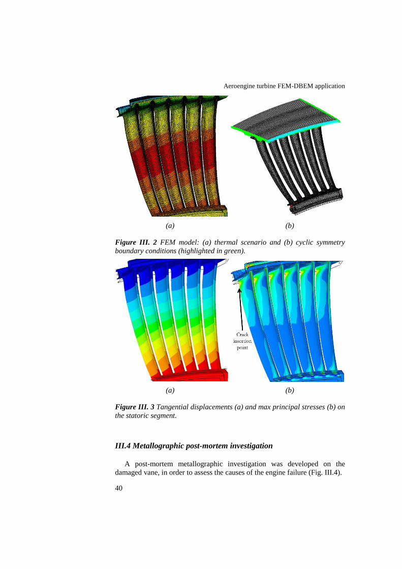
Aeroengine turbine FEM-DBEM application

40

(a) (b)

Figure III. 2 FEM model: (a) thermal scenario and (b) cyclic symmetry

boundary conditions (highlighted in green).

(a) (b)

Figure III. 3 Tangential displacements (a) and max principal stresses (b) on

the statoric segment.

III.4 Metallographic post-mortem investigation

A post-mortem metallographic investigation was developed on the

damaged vane, in order to assess the causes of the engine failure (Fig. III.4).

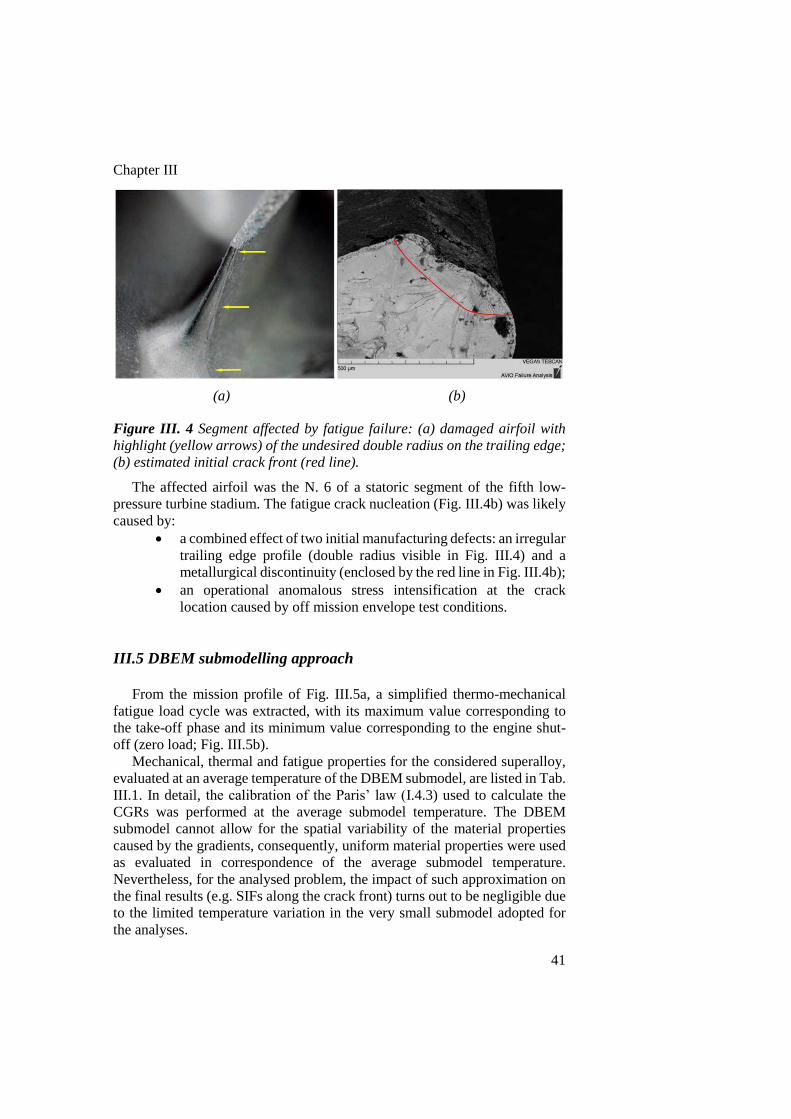
Chapter III

41

(a) (b)

Figure III. 4 Segment affected by fatigue failure: (a) damaged airfoil with

highlight (yellow arrows) of the undesired double radius on the trailing edge;

(b) estimated initial crack front (red line).

The affected airfoil was the N. 6 of a statoric segment of the fifth low-

pressure turbine stadium. The fatigue crack nucleation (Fig. III.4b) was likely

caused by:

a combined effect of two initial manufacturing defects: an irregular

trailing edge profile (double radius visible in Fig. III.4) and a

metallurgical discontinuity (enclosed by the red line in Fig. III.4b);

an operational anomalous stress intensification at the crack

location caused by off mission envelope test conditions.

III.5 DBEM submodelling approach

From the mission profile of Fig. III.5a, a simplified thermo-mechanical

fatigue load cycle was extracted, with its maximum value corresponding to

the take-off phase and its minimum value corresponding to the engine shut-

off (zero load; Fig. III.5b).

Mechanical, thermal and fatigue properties for the considered superalloy,

evaluated at an average temperature of the DBEM submodel, are listed in Tab.

III.1. In detail, the calibration of the Paris’ law (I.4.3) used to calculate the

CGRs was performed at the average submodel temperature. The DBEM

submodel cannot allow for the spatial variability of the material properties

caused by the gradients, consequently, uniform material properties were used

as evaluated in correspondence of the average submodel temperature.

Nevertheless, for the analysed problem, the impact of such approximation on

the final results (e.g. SIFs along the crack front) turns out to be negligible due

to the limited temperature variation in the very small submodel adopted for

the analyses.

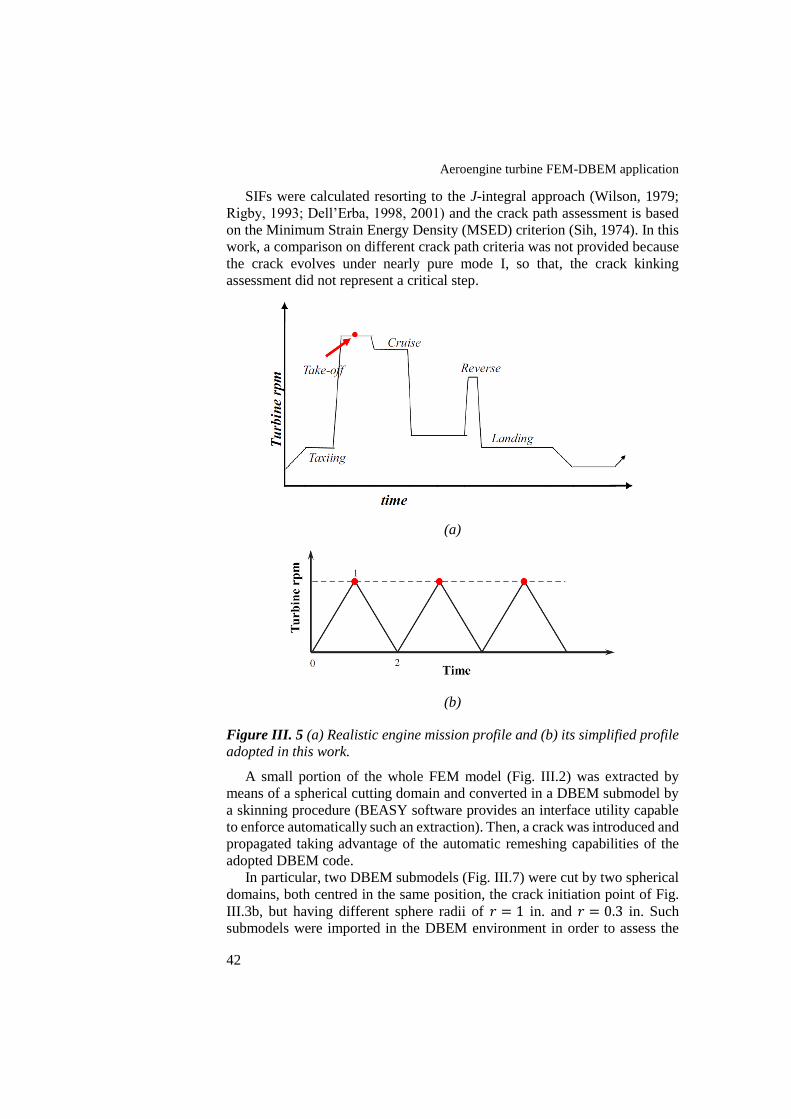
Aeroengine turbine FEM-DBEM application

42

SIFs were calculated resorting to the J-integral approach (Wilson, 1979;

Rigby, 1993; Dell’Erba, 1998, 2001) and the crack path assessment is based

on the Minimum Strain Energy Density (MSED) criterion (Sih, 1974). In this

work, a comparison on different crack path criteria was not provided because

the crack evolves under nearly pure mode I, so that, the crack kinking

assessment did not represent a critical step.

(a)

(b)

Figure III. 5 (a) Realistic engine mission profile and (b) its simplified profile

adopted in this work.

A small portion of the whole FEM model (Fig. III.2) was extracted by

means of a spherical cutting domain and converted in a DBEM submodel by

a skinning procedure (BEASY software provides an interface utility capable

to enforce automatically such an extraction). Then, a crack was introduced and

propagated taking advantage of the automatic remeshing capabilities of the

adopted DBEM code.

In particular, two DBEM submodels (Fig. III.7) were cut by two spherical

domains, both centred in the same position, the crack initiation point of Fig.

III.3b, but having different sphere radii of 𝑟 = 1 in. and 𝑟 = 0.3 in. Such

submodels were imported in the DBEM environment in order to assess the

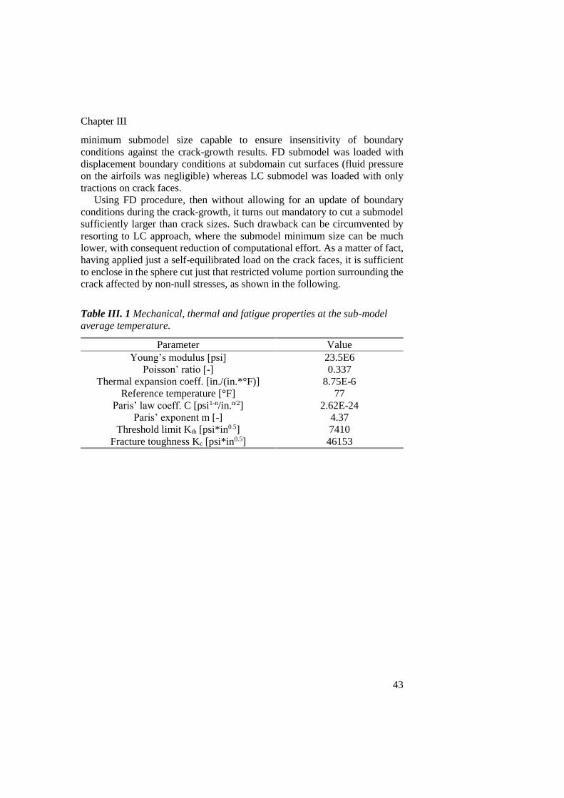
Chapter III

43

minimum submodel size capable to ensure insensitivity of boundary

conditions against the crack-growth results. FD submodel was loaded with

displacement boundary conditions at subdomain cut surfaces (fluid pressure

on the airfoils was negligible) whereas LC submodel was loaded with only

tractions on crack faces.

Using FD procedure, then without allowing for an update of boundary

conditions during the crack-growth, it turns out mandatory to cut a submodel

sufficiently larger than crack sizes. Such drawback can be circumvented by

resorting to LC approach, where the submodel minimum size can be much

lower, with consequent reduction of computational effort. As a matter of fact,

having applied just a self-equilibrated load on the crack faces, it is sufficient

to enclose in the sphere cut just that restricted volume portion surrounding the

crack affected by non-null stresses, as shown in the following.

Table III. 1 Mechanical, thermal and fatigue properties at the sub-model

average temperature.

Parameter Value

Young’s modulus [psi] 23.5E6

Poisson’ ratio [-] 0.337

Thermal expansion coeff. [in./(in.*°F)] 8.75E-6

Reference temperature [°F] 77

Paris’ law coeff. C [psi1-n/in.n/2] 2.62E-24

Paris’ exponent m [-] 4.37

Threshold limit Kth [psi*in0.5] 7410

Fracture toughness Kc [psi*in0.5] 46153

Aeroengine turbine FEM-DBEM application

44

(a) (b)

Figure III. 6 Considered loading strategies for DBEM analyses: (a) LC and

(b) FD; model for LC comprises the self-equilibrated load on the crack face

elements and few constraints to prevent rigid body motion; model for FD

comprises temperature on all the elements and displacement field on all the

cut surface elements.

Figure III. 7 Max principal stresses before crack introduction on the two

DBEM submodels used for FD approach; highlight of the crack insertion

position.

Chapter III

45

III.6 Results

The first goal was to assess the minimum required submodel size

“compatible” with the boundary conditions that were updated or not during

crack-growth for LC and FD respectively. In more details, submodel boundary

conditions for both FD and LC approaches come from the FEM analysis of

the uncracked global model but, for the FD approach, this represents an

element of approximation. In fact, the displacement boundary conditions

applied on the cutting surfaces should, in principle, be updated at each step of

crack advance, to allow for the submodel stiffness variation when solving the

global model. On the contrary, with the LC approach, the self-equilibrated

tractions applied on both faces of the crack are correctly extracted from an

uncracked body solution, as rigorous dictated by the superposition principle

implementation (§I.2). Moreover, such tractions are updated step-by-step

because new crack surfaces are continuously created and loaded during the

crack-growth simulation. Thus, for LC approach there is no need to guarantee

a submodel much larger than the crack extension, being sufficient to enclose

the volume surrounding the crack with non-zero stresses; such stress ‘‘fading

distance” can be very short because of a self-equilibrated load applied to the

model.

The crack representing the initial detected defect (red line in Fig. III.4b)

was modelled and inserted in both LC and FD DBEM submodels. Introducing

the crack into DBEM submodels, with the inherent automatic remeshing of

the cracked surroundings, two different stress scenarios came out from FD and

LC approaches (Fig. III.8): the former produces a realistic stress scenario

throughout the whole DBEM submodel whereas the latter is meaningful only

for the SIFs evaluation. Hence, a comparison between the two methodologies

can just involve SIFs along the crack front and, therefore, the CGRs and kink

angles that are directly connected to the SIFs calculation.

Aeroengine turbine FEM-DBEM application

46

Figure III. 8 Von Mises stresses [psi] for the initial cracked FD (a) and LC

(b) models, with close-up of the cracked area (cutting sphere radius R = 1

in.).

A convergence study (Fig. III.9-10) was performed for both the FD and LC

methodologies, varying the submodel size and the mesh refinement on and

nearby the crack (Fig. III.9), in order to benchmark the respective convergence

rates and computational efficiencies. Analysing the so obtained SIFs, it was

possible to observe a high convergence rate of LC methodology (Fig. III.10a),

rapidly providing a convergent SIF distribution along the crack front even for

coarse meshes, i.e. with high crack front element size (hereinafter “cfes”,

BEASY, 2011) values. On the contrary, the FD methodology needed strong

mesh refinements (Fig. III.10b) to get convergent results but, anyhow,

perfectly coincident SIFs could not even be obtained since too fine meshes

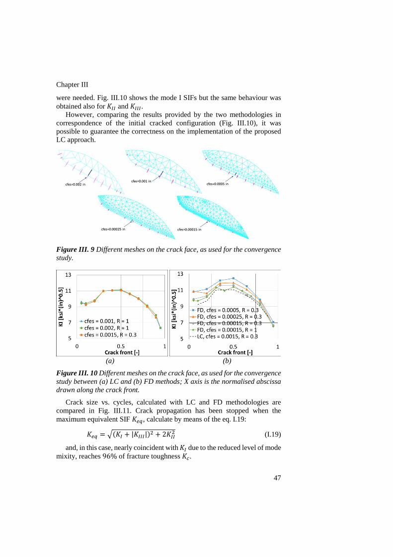
Chapter III

47

were needed. Fig. III.10 shows the mode I SIFs but the same behaviour was

obtained also for 𝐾𝐼𝐼 and 𝐾𝐼𝐼𝐼.

However, comparing the results provided by the two methodologies in

correspondence of the initial cracked configuration (Fig. III.10), it was

possible to guarantee the correctness on the implementation of the proposed

LC approach.

Figure III. 9 Different meshes on the crack face, as used for the convergence

study.

(a) (b)

Figure III. 10 Different meshes on the crack face, as used for the convergence

study between (a) LC and (b) FD methods; X axis is the normalised abscissa

drawn along the crack front.

Crack size vs. cycles, calculated with LC and FD methodologies are

compared in Fig. III.11. Crack propagation has been stopped when the

maximum equivalent SIF 𝐾𝑒𝑞, calculate by means of the eq. I.19:

𝐾𝑒𝑞 = √(𝐾𝐼 + |𝐾𝐼𝐼𝐼|)2 + 2𝐾𝐼𝐼2 (I.19)

and, in this case, nearly coincident with 𝐾𝐼 due to the reduced level of mode

mixity, reaches 96% of fracture toughness 𝐾𝑐.

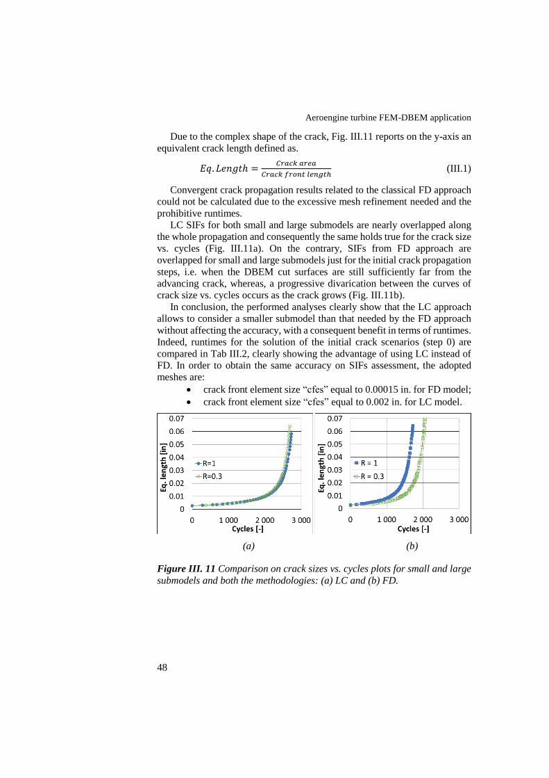
Aeroengine turbine FEM-DBEM application

48

Due to the complex shape of the crack, Fig. III.11 reports on the y-axis an

equivalent crack length defined as.

𝐸𝑞. 𝐿𝑒𝑛𝑔𝑡ℎ =𝐶𝑟𝑎𝑐𝑘 𝑎𝑟𝑒𝑎

𝐶𝑟𝑎𝑐𝑘 𝑓𝑟𝑜𝑛𝑡 𝑙𝑒𝑛𝑔𝑡ℎ (III.1)

Convergent crack propagation results related to the classical FD approach

could not be calculated due to the excessive mesh refinement needed and the

prohibitive runtimes.

LC SIFs for both small and large submodels are nearly overlapped along

the whole propagation and consequently the same holds true for the crack size

vs. cycles (Fig. III.11a). On the contrary, SIFs from FD approach are

overlapped for small and large submodels just for the initial crack propagation

steps, i.e. when the DBEM cut surfaces are still sufficiently far from the

advancing crack, whereas, a progressive divarication between the curves of

crack size vs. cycles occurs as the crack grows (Fig. III.11b).

In conclusion, the performed analyses clearly show that the LC approach

allows to consider a smaller submodel than that needed by the FD approach

without affecting the accuracy, with a consequent benefit in terms of runtimes.

Indeed, runtimes for the solution of the initial crack scenarios (step 0) are

compared in Tab III.2, clearly showing the advantage of using LC instead of

FD. In order to obtain the same accuracy on SIFs assessment, the adopted

meshes are:

crack front element size “cfes” equal to 0.00015 in. for FD model;

crack front element size “cfes” equal to 0.002 in. for LC model.

(a) (b)

Figure III. 11 Comparison on crack sizes vs. cycles plots for small and large

submodels and both the methodologies: (a) LC and (b) FD.

Chapter III

49

Table III. 2 Runtimes compared for FD and LC approaches.

- DOFs x103 Step 0 solving phase [min]

FD, r = 1 in. 109 773

LC, r = 1 in. 33 22

FD, r = 0.3 in. 68 224

LC, r = 0.3 in. 14 7

III.7 Remarks

An enhanced FEM-DBEM submodelling approach, based on the principle

of linear superposition to solve fracture problems, has been implemented for

a crack-growth simulation in a GE-AVIO aeroengine turbine vane. A

benchmark of such enhanced LC approach against a classical FD procedure

has been proposed and the advantages in terms of runtimes and accuracy are

summarized in the following:

LC approach is fully automated and permits to predict SIF, then

also CGRs and kink angles, with higher accuracy and lower

runtimes than for FD approach.

LC approach allows a remarkable decrease in terms of runtimes

for SIF calculations because resorting to pure stress analyses

instead of, in this case, thermal-stress analyses (needed for the FD

procedure), also needing a less refined mesh to get convergent

results.

LC approach accuracy is enhanced because the boundary

conditions on the advancing crack are theoretically “correct” since

they are correctly extracted from an uncracked FEM global model,

as dictated by the superposition principle. Moreover, this allows

also considering continuously updating boundary conditions

during the simulation, whereas the FD approach is based on

boundary conditions with no update during propagation (even if

such update would be theoretically needed).

LC guarantees a lower sensitivity of results against the distance

between the cutting surfaces and crack as proven considering

different submodel sizes.

The fine tuning of crack propagation parameters with the FD

procedure is more complex because of two contrasting

requirements during a crack-growth simulation: a coarse mesh in

order to facilitate the remeshing procedure and, at the same time,

a very fine mesh in order to guarantee sufficient accuracy for SIFs

calculations.

Aeroengine turbine FEM-DBEM application

50

Future developments of present activity will concern an introduction of

more realistic fatigue spectrum, representative of more phases of the turbine

engine mission profile (Fig. III.5).

Chapter IV

FEM-DBEM application on

Wendelstein 7-X structure

IV.1 Introduction

In this paragraph a realistic fatigue life assessment of a structural element

of the supporting structure of the machine for the fusion experiment

“Wendelstein 7-X” (W7-X) is presented. In particular, several cracks were

detected on a Lateral Support Element (LSE) of the W7-X machine and the

most critical crack has been here analysed by three distinct FEM-DBEM

approaches (§II.2.3): Fixed Displacements (FD), Fixed Loads (FL) and

Loaded Crack (LC). Two complex fatigue spectra were adopted to realistically

reproduce the operating conditions of the machine. We will show how FD and

FL approaches provide an upper and a lower bound for fatigue life predictions,

whereas the LC results lye in between such bounds, confirming again that LC

approach represents an accurate submodelling strategy by means of which it

is possible to solve a generic fracture problem. Further details can be found in

the literature (Giannella, 2017a).

IV.2 Problem description

Wendelstein 7-X (W7-X) is the world’s largest nuclear fusion experiment

of stellarator type (Spitzer, 21958; Xu, 2016) that started operation in 2015 at

the Max-Planck-Institute for Plasma-Physics in Greifswald, Germany (Fig.

IV.1a; Wolf, 2017). In the machine, a hot helium or hydrogen plasma is

confined in a Plasma Vessel (PV) by means of an electromagnetic (EM) field

(Fig. IV.1b), reaching a magnitude up to 3 T, provided by 50 non-planar and

20 planar superconducting coils (Fig. IV.1c). In the vacuum created inside the

cryostat, the coils are cooled down to a superconducting temperature, close to

absolute zero (4 K), using liquid helium. The magnetic cage keeps the 30 cubic

metres of ultra-thin plasma suspended inside the PV. Such plasma is heated

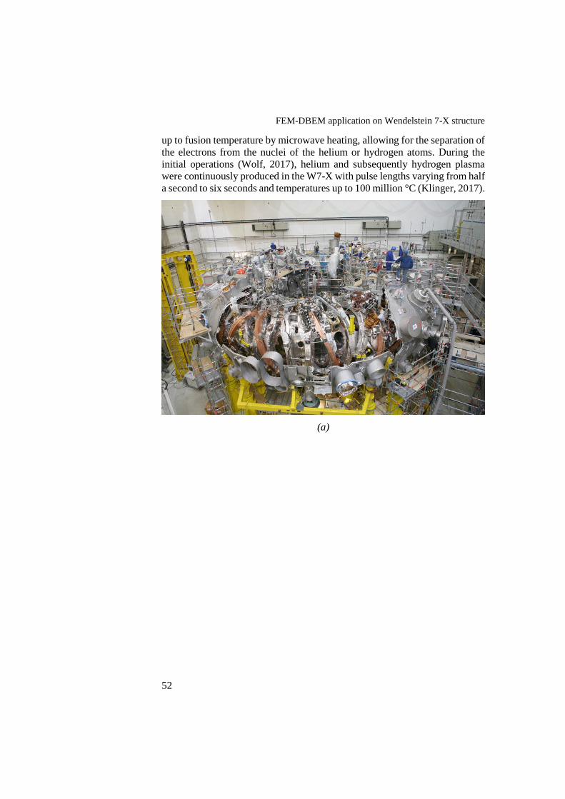
FEM-DBEM application on Wendelstein 7-X structure

52

up to fusion temperature by microwave heating, allowing for the separation of

the electrons from the nuclei of the helium or hydrogen atoms. During the

initial operations (Wolf, 2017), helium and subsequently hydrogen plasma

were continuously produced in the W7-X with pulse lengths varying from half

a second to six seconds and temperatures up to 100 million °C (Klinger, 2017).

(a)

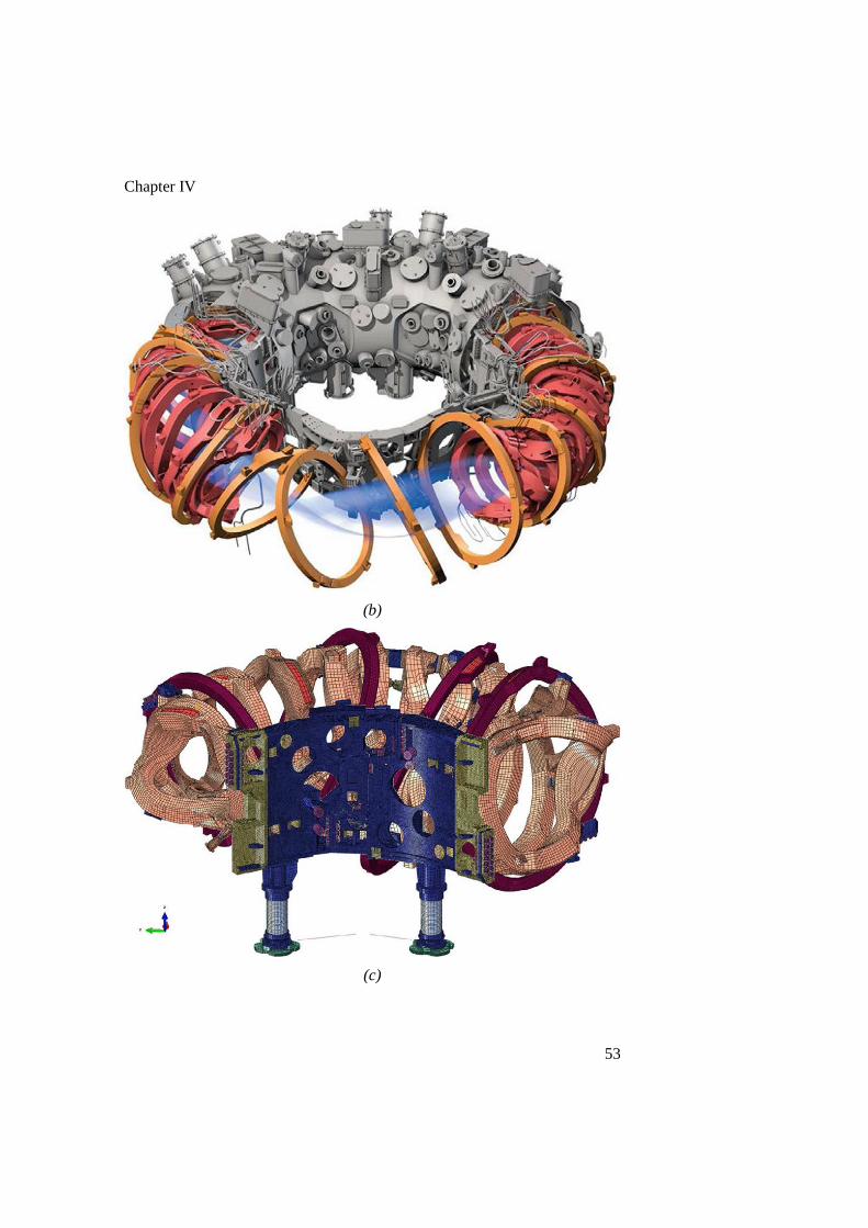
Chapter IV

53

(b)

(c)

FEM-DBEM application on Wendelstein 7-X structure

54

(d)

Figure IV. 1 (a) Modular-type stellarator Wendelstein 7-X; (b) Hot plasma

confined by EM field generated by the coils; (c) FEM assembly of one-fifth of

the magnet system of W7-X; (d) W7-X magnet system: FEM detail of a half

module with the LSEs; highlights on the investigated LSE-05.

The superconducting coils are bolted onto a central support ring and

interconnected by welded Lateral Support Elements (LSEs; Fig. IV.1d): 100–

150 mm long hollow tubes of 30–35 mm thickness made of forged stainless

steel (EN 1.4429).

After the welding of the LSEs to the coil cases (weld depth 15–30 mm),

several surface cracks larger than 8 mm (typical acceptance limit of EN 23277,

2010) were found near the welds that could potentially limit the W7-X

operations. Cracks were found with visual inspection and dye penetration tests

at the accessible surfaces, particularly at the coil side of the weld within the

cast steel, oriented mainly parallel to the weld seam (Fig. IV.2). Such cracks,

in coils and superconducting cables areas where high stresses develop (Corato,

2015), can become critical during operations.

In order to take advantage of the high accuracy and flexibility of DBEM

(Kuranakov, 2016; Alatawi, 2015; Chen, 1999; Hong, 1988) when handling

3D crack-growth under mixed-mode conditions, in (Citarella, 2013) such

cracks were modelled using a coupled FEM-DBEM approach (Citarella, 2014,

2016b, 2016c). Crack sizes as well as stress-states and SIFs along the crack

front were step-by-step updated through the entire simulation, and the crack-

growth was continued until the critical SIF was reached. The crack depth was

not pointed out by NDI (Non-Destructive Inspection) tests; however, from

repair experience it was found that such size is typically smaller than half the

superficial crack length. In (Citarella, 2016c), the same problem was tackled

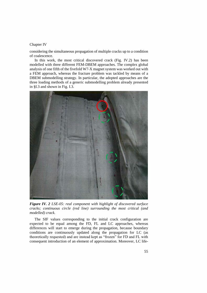
Chapter IV

55

considering the simultaneous propagation of multiple cracks up to a condition

of coalescence.

In this work, the most critical discovered crack (Fig. IV.2) has been

modelled with three different FEM-DBEM approaches. The complex global

analysis of one fifth of the fivefold W7-X magnet system was worked out with

a FEM approach, whereas the fracture problem was tackled by means of a

DBEM submodelling strategy. In particular, the adopted approaches are the

three loading methods of a generic submodelling problem already presented

in §I.3 and shown in Fig. I.3.

Figure IV. 2 LSE-05: real component with highlight of discovered surface

cracks; continuous circle (red line) surrounding the most critical (and

modelled) crack.

The SIF values corresponding to the initial crack configuration are

expected to be equal among the FD, FL and LC approaches, whereas

differences will start to emerge during the propagation, because boundary

conditions are continuously updated along the propagation for LC (as

theoretically requested) and are instead kept as “frozen” for FD and FL with

consequent introduction of an element of approximation. Moreover, LC life-

FEM-DBEM application on Wendelstein 7-X structure

56

prediction is expected to be in between the predictions computed by FD and

FL approaches.

The ABAQUS (ABAQUS, 2011) and BEASY (BEASY, 2011)

commercial codes are used for FEM and DBEM analyses respectively.

IV.3 FEM modelling

A global FEM model of one fifth of the fivefold symmetric W7-X magnetic

cage has been developed (Fig. IV.3a) considering, in addition to the magnetic

loads (“HJ” refers to the most critical magnetic field configuration, better

explained in §IV.5): bolt preloading, dead weight and cooling. Then, a first

FEM submodel (Fig. IV.3b) involving the whole LSE-05 (Fig. IV.3b) has

been made (without any crack introduction). In final, a second FEM submodel,

involving a smaller part of LSE-05, has been built up (Fig. IV.3c) in order to

get a more accurate stress assessment on the cracked area. Namely, with such

submodel it has been possible to provide more accurate stress field to load the

DBEM crack faces, as requested by the LC approach.

(a)

Chapter IV

57

(b)

(c)

Figure IV. 3 Von Mises stresses [Pa], related to the load case with EM field

of 3 T “HJ”, on the: (a) FEM global model, (b) first FEM LSE-05 submodel,

(c) furtherly reduced FEM submodel. Red arrow in (a) pointing out the

submodelled LSE-05 in (b). Dashed red square in (b) representing the area

that has been furtherly refined in (c).

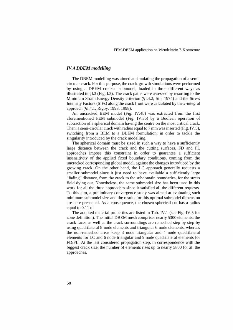
FEM-DBEM application on Wendelstein 7-X structure

58

IV.4 DBEM modelling

The DBEM modelling was aimed at simulating the propagation of a semi-

circular crack. For this purpose, the crack-growth simulations were performed

by using a DBEM cracked submodel, loaded in three different ways as

illustrated in §I.3 (Fig. I.3). The crack paths were assessed by resorting to the

Minimum Strain Energy Density criterion (§I.4.2; Sih, 1974) and the Stress

Intensity Factors (SIFs) along the crack front were calculated by the J-integral

approach (§I.4.1; Rigby, 1993, 1998).

An uncracked BEM model (Fig. IV.4b) was extracted from the first

aforementioned FEM submodel (Fig. IV.3b) by a Boolean operation of

subtraction of a spherical domain having the centre on the most critical crack.

Then, a semi-circular crack with radius equal to 7 mm was inserted (Fig. IV.5),

switching from a BEM to a DBEM formulation, in order to tackle the

singularity introduced by the crack modelling.

The spherical domain must be sized in such a way to have a sufficiently

large distance between the crack and the cutting surfaces. FD and FL

approaches impose this constraint in order to guarantee a sufficient

insensitivity of the applied fixed boundary conditions, coming from the

uncracked corresponding global model, against the changes introduced by the

growing crack. On the other hand, the LC approach generally requests a

smaller submodel since it just need to have available a sufficiently large

“fading” distance, from the crack to the subdomain boundaries, for the stress

field dying out. Nonetheless, the same submodel size has been used in this

work for all the three approaches since it satisfied all the different requests.

To this aim, a preliminary convergence study was aimed at evaluating such

minimum submodel size and the results for this optimal submodel dimension

are here presented. As a consequence, the chosen spherical cut has a radius

equal to 0.11 m.

The adopted material properties are listed in Tab. IV.1 (see Fig. IV.5 for

zone definition). The initial DBEM mesh comprises nearly 5300 elements: the

crack faces as well as the crack surroundings are remeshed step-by-step by

using quadrilateral 8-node elements and triangular 6-node elements, whereas

the non-remeshed areas keep 3 node triangular and 4 node quadrilateral

elements for LC and 6 node triangular and 9 node quadrilateral elements for

FD/FL. At the last considered propagation step, in correspondence with the

biggest crack size, the number of elements rises up to nearly 5800 for all the

approaches.

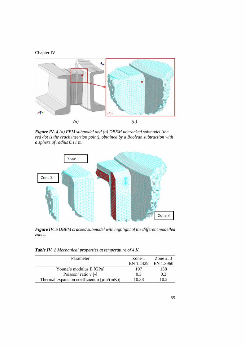
Chapter IV

59

(a) (b)

Figure IV. 4 (a) FEM submodel and (b) DBEM uncracked submodel (the

red dot is the crack insertion point), obtained by a Boolean subtraction with

a sphere of radius 0.11 m.

Figure IV. 5 DBEM cracked submodel with highlight of the different modelled

zones.

Table IV. 1 Mechanical properties at temperature of 4 K.

Parameter Zone 1

EN 1.4429

Zone 2, 3

EN 1.3960

Young’s modulus E [GPa] 197 158

Poisson’ ratio ν [-] 0.3 0.3

Thermal expansion coefficient α [µm/(mK)] 10.38 10.2

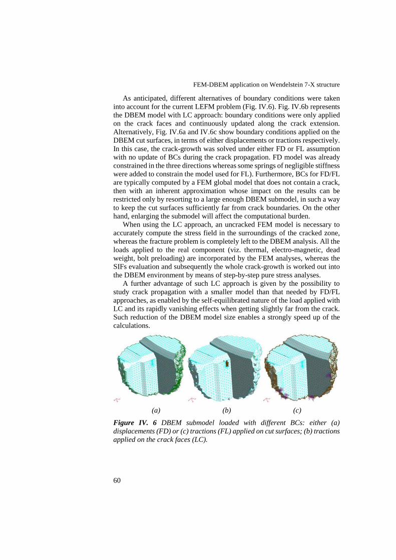
FEM-DBEM application on Wendelstein 7-X structure

60

As anticipated, different alternatives of boundary conditions were taken

into account for the current LEFM problem (Fig. IV.6). Fig. IV.6b represents

the DBEM model with LC approach: boundary conditions were only applied

on the crack faces and continuously updated along the crack extension.

Alternatively, Fig. IV.6a and IV.6c show boundary conditions applied on the

DBEM cut surfaces, in terms of either displacements or tractions respectively.

In this case, the crack-growth was solved under either FD or FL assumption

with no update of BCs during the crack propagation. FD model was already

constrained in the three directions whereas some springs of negligible stiffness

were added to constrain the model used for FL). Furthermore, BCs for FD/FL

are typically computed by a FEM global model that does not contain a crack,

then with an inherent approximation whose impact on the results can be

restricted only by resorting to a large enough DBEM submodel, in such a way

to keep the cut surfaces sufficiently far from crack boundaries. On the other

hand, enlarging the submodel will affect the computational burden.

When using the LC approach, an uncracked FEM model is necessary to

accurately compute the stress field in the surroundings of the cracked zone,

whereas the fracture problem is completely left to the DBEM analysis. All the

loads applied to the real component (viz. thermal, electro-magnetic, dead

weight, bolt preloading) are incorporated by the FEM analyses, whereas the

SIFs evaluation and subsequently the whole crack-growth is worked out into

the DBEM environment by means of step-by-step pure stress analyses.

A further advantage of such LC approach is given by the possibility to

study crack propagation with a smaller model than that needed by FD/FL

approaches, as enabled by the self-equilibrated nature of the load applied with

LC and its rapidly vanishing effects when getting slightly far from the crack.

Such reduction of the DBEM model size enables a strongly speed up of the

calculations.

(a) (b) (c)

Figure IV. 6 DBEM submodel loaded with different BCs: either (a)

displacements (FD) or (c) tractions (FL) applied on cut surfaces; (b) tractions

applied on the crack faces (LC).

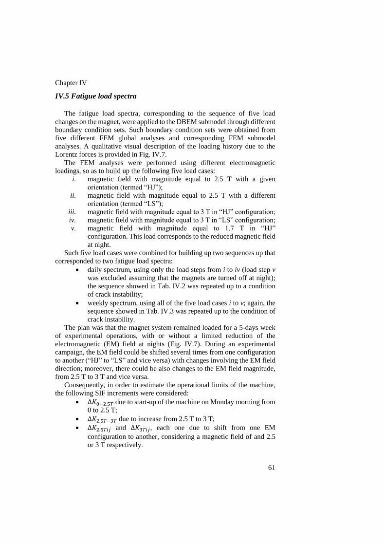
Chapter IV

61

IV.5 Fatigue load spectra

The fatigue load spectra, corresponding to the sequence of five load

changes on the magnet, were applied to the DBEM submodel through different

boundary condition sets. Such boundary condition sets were obtained from

five different FEM global analyses and corresponding FEM submodel

analyses. A qualitative visual description of the loading history due to the

Lorentz forces is provided in Fig. IV.7.

The FEM analyses were performed using different electromagnetic

loadings, so as to build up the following five load cases:

i. magnetic field with magnitude equal to 2.5 T with a given

orientation (termed “HJ”);

ii. magnetic field with magnitude equal to 2.5 T with a different

orientation (termed “LS”);

iii. magnetic field with magnitude equal to 3 T in “HJ” configuration;

iv. magnetic field with magnitude equal to 3 T in “LS” configuration;

v. magnetic field with magnitude equal to 1.7 T in “HJ”

configuration. This load corresponds to the reduced magnetic field

at night.

Such five load cases were combined for building up two sequences up that

corresponded to two fatigue load spectra:

daily spectrum, using only the load steps from i to iv (load step v

was excluded assuming that the magnets are turned off at night);

the sequence showed in Tab. IV.2 was repeated up to a condition

of crack instability;

weekly spectrum, using all of the five load cases i to v; again, the

sequence showed in Tab. IV.3 was repeated up to the condition of

crack instability.

The plan was that the magnet system remained loaded for a 5-days week

of experimental operations, with or without a limited reduction of the

electromagnetic (EM) field at nights (Fig. IV.7). During an experimental

campaign, the EM field could be shifted several times from one configuration

to another (“HJ” to “LS” and vice versa) with changes involving the EM field

direction; moreover, there could be also changes to the EM field magnitude,

from 2.5 T to 3 T and vice versa.

Consequently, in order to estimate the operational limits of the machine,

the following SIF increments were considered:

∆𝐾0−2.5𝑇 due to start-up of the machine on Monday morning from

0 to 2.5 T;

∆𝐾2.5𝑇−3𝑇 due to increase from 2.5 T to 3 T;

∆𝐾2.5𝑇𝑖𝑗 and ∆𝐾3𝑇𝑖𝑗, each one due to shift from one EM

configuration to another, considering a magnetic field of and 2.5

or 3 T respectively.

FEM-DBEM application on Wendelstein 7-X structure

62

In case of weekly spectrum, ∆𝐾𝑛𝑖𝑔ℎ𝑡, related to a moderate reduction of

the magnetic field at night, was added. Changes in the EM field for plasma

ripple control were considered as small enough to be neglected.

Figure IV. 7 Schematic loading history due to EM forces.

Table IV. 2 Fatigue elementary block corresponding to 10 working days

with the daily spectrum (12.1 cycles per working day).

Cycles per

block

EM field (minimum

magnitude)

EM field (maximum

magnitude)

10 0 2.5 T (“HJ” config.)

100 2.5 T (“LS” config.) 2.5 T (“HJ” config.)

1 0 3 T (“HJ” config.)

10 3 T (“LS” config.) 3 T (“HJ” config.)

Table IV. 3 Fatigue elementary block corresponding to 50 working days

with the weekly spectrum (5.42 cycles per working day).

Cycles per

block

EM field (minimum

magnitude)

EM field (maximum

magnitude)

10 0 2.5 T (“HJ” config.)

200 2.5 T (“LS” config.) 2.5 T (“HJ” config.)

1 0 3 T (“HJ” config.)

20 3 T (“LS” config.) 3 T (“HJ” config.)

40 1.7 T (“HJ” config.) 2.5 T (“HJ” config.)

The crack-growth for the load cycles from 0 to 2.5 T was predicted by

using a Paris’ law (§I.4.3; Paris, 1961):

𝑑𝑎

𝑑𝑁= 𝐶∆𝐾𝑚 (I.15)

with the related Paris’ parameters listed in Tab. IV.4, as derived from

Fatigue Crack-Growth Rate (FCGR) test series carried out at cryogenic

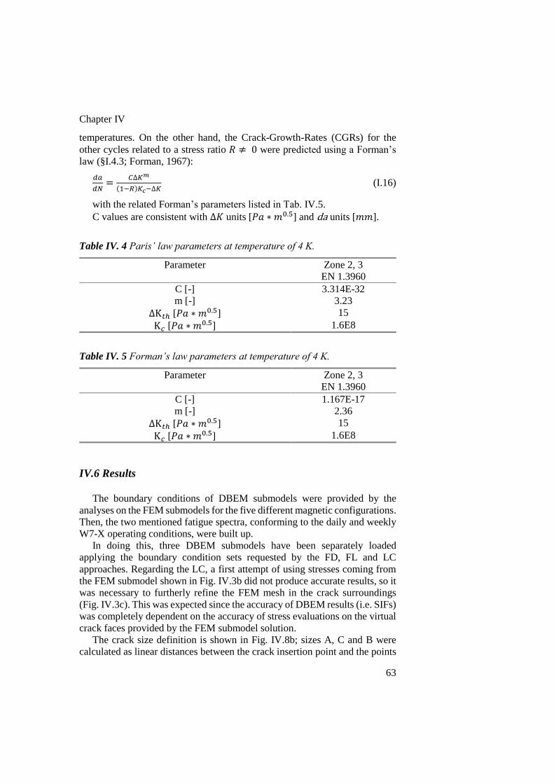
Chapter IV

63

temperatures. On the other hand, the Crack-Growth-Rates (CGRs) for the

other cycles related to a stress ratio 𝑅 ≠ 0 were predicted using a Forman’s

law (§I.4.3; Forman, 1967):

𝑑𝑎

𝑑𝑁=

𝐶∆𝐾𝑚

(1−𝑅)𝐾𝑐−∆𝐾 (I.16)

with the related Forman’s parameters listed in Tab. IV.5.

C values are consistent with ∆𝐾 units [𝑃𝑎 ∗ 𝑚0.5] and da units [𝑚𝑚].

Table IV. 4 Paris’ law parameters at temperature of 4 K.

Parameter Zone 2, 3

EN 1.3960

C [-] 3.314E-32

m [-] 3.23

∆K𝑡ℎ [𝑃𝑎 ∗ 𝑚0.5] 15

K𝑐 [𝑃𝑎 ∗ 𝑚0.5] 1.6E8

Table IV. 5 Forman’s law parameters at temperature of 4 K.

Parameter Zone 2, 3

EN 1.3960

C [-] 1.167E-17

m [-] 2.36

∆K𝑡ℎ [𝑃𝑎 ∗ 𝑚0.5] 15

K𝑐 [𝑃𝑎 ∗ 𝑚0.5] 1.6E8

IV.6 Results

The boundary conditions of DBEM submodels were provided by the

analyses on the FEM submodels for the five different magnetic configurations.

Then, the two mentioned fatigue spectra, conforming to the daily and weekly

W7-X operating conditions, were built up.

In doing this, three DBEM submodels have been separately loaded

applying the boundary condition sets requested by the FD, FL and LC

approaches. Regarding the LC, a first attempt of using stresses coming from

the FEM submodel shown in Fig. IV.3b did not produce accurate results, so it

was necessary to furtherly refine the FEM mesh in the crack surroundings

(Fig. IV.3c). This was expected since the accuracy of DBEM results (i.e. SIFs)

was completely dependent on the accuracy of stress evaluations on the virtual

crack faces provided by the FEM submodel solution.

The crack size definition is shown in Fig. IV.8b; sizes A, C and B were

calculated as linear distances between the crack insertion point and the points

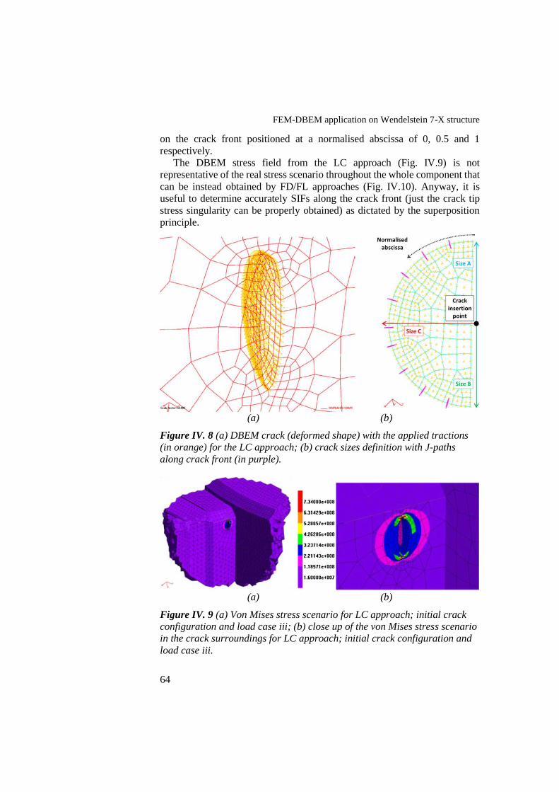
FEM-DBEM application on Wendelstein 7-X structure

64

on the crack front positioned at a normalised abscissa of 0, 0.5 and 1

respectively.

The DBEM stress field from the LC approach (Fig. IV.9) is not

representative of the real stress scenario throughout the whole component that

can be instead obtained by FD/FL approaches (Fig. IV.10). Anyway, it is

useful to determine accurately SIFs along the crack front (just the crack tip

stress singularity can be properly obtained) as dictated by the superposition

principle.

(a) (b)

Figure IV. 8 (a) DBEM crack (deformed shape) with the applied tractions

(in orange) for the LC approach; (b) crack sizes definition with J-paths

along crack front (in purple).

(a) (b)

Figure IV. 9 (a) Von Mises stress scenario for LC approach; initial crack

configuration and load case iii; (b) close up of the von Mises stress scenario

in the crack surroundings for LC approach; initial crack configuration and

load case iii.

Chapter IV

65

Figure IV. 10 Von Mises stress scenario from FD/FL approach; initial crack

configuration and load case iii.

SIFs computed by the three approaches are compared in Fig. IV.11 for all

the five different load cases from i to v. Such SIFs for the initial crack

configuration show a perfect match between the adopted approaches, proving

also the correct implementation of the superposition principle to the

considered LEFM problem.

Once the FEM analyses were completed and the DBEM submodel created

and loaded, step-by-step crack-growths were simulated. Each single growth

step was comprehensive of the following phases:

1) crack insertion;

2) crack faces loading (needed only by the LC approach);

3) linear-elastic DBEM analysis and corresponding SIFs evaluation;

4) life prediction;

5) new crack front prediction.

As previously said, the application of either traction (FL) or displacement

(FD) boundary conditions to the DBEM cut surfaces would represent an

approximation due to the continuously increasing crack dimensions and the

consequential continuously decreasing DBEM model stiffness. In addition,

such boundary conditions generally come from a FEM global model in which

the presence of the crack is not considered at all. On the contrary, the LC

approach does not present such approximations, as the traction boundary

conditions applied on the crack faces are rigorously computed from an

uncracked FEM domain, as theoretically dictated by the superposition

principle. In addition, such crack faces loads are continuously updated through

the simulation since further loads are applied on the continuously created

crack extensions.

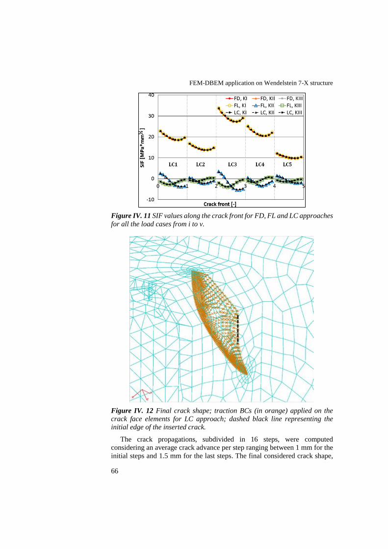
FEM-DBEM application on Wendelstein 7-X structure

66

Figure IV. 11 SIF values along the crack front for FD, FL and LC approaches

for all the load cases from i to v.

Figure IV. 12 Final crack shape; traction BCs (in orange) applied on the

crack face elements for LC approach; dashed black line representing the

initial edge of the inserted crack.

The crack propagations, subdivided in 16 steps, were computed

considering an average crack advance per step ranging between 1 mm for the

initial steps and 1.5 mm for the last steps. The final considered crack shape,

Chapter IV

67

with the related tractions applied on the crack face elements for LC, is shown

in Fig. IV.12: a slight kinking of the growing crack is visible consistently with

the slight mixed-mode conditions shown in Fig. IV.11.

Results in terms of crack advance vs. fatigue cycles and 𝐾𝑒𝑞 during growth

for both daily and weekly fatigue spectra are reported in Figs. IV.13 and IV.14

respectively: it is possible to observe that the 𝐾𝑒𝑞 values, even if higher than

threshold, turn out to be lower than 𝐾𝑐 up to the final considered scenario,

which consequently was judged subcritical.

Equivalent SIF values were computed by using the Yaoming-Mi formula

(§I.4.3; Mi, 1995):

𝐾𝑒𝑞 = √(𝐾𝐼 + |𝐾𝐼𝐼𝐼|)2 + 2𝐾𝐼𝐼2 (I.19)

and its variation in the cycle provided the ∆𝐾𝑒𝑞 to be used in the Paris’ and

Forman’s laws (eqs. I.14 and I.15).

From fig. IV.13, it is possible to observe the progressively increasing

difference between the three approaches, dictated by SIF values that are

precisely overlapped at the initial step (step 0; Fig. IV.11) and progressively

diverging along with the crack extension (Fig. IV.14).

Daily and weekly load spectra appeared to give quite similar fatigue life

predictions, as visible from Fig. IV.13, but differences came out if considering

on the abscissa the working days rather than the fatigue cycles. As a matter of

fact, the daily spectrum predicted a much lower number of working days,

before than reaching a critical condition, because the EM field was considered

as turned down at night, with consequent less frequent main cycles (those

related to the switch-off of the EM field with corresponding strongest

variation on SIFs).

In final, a comparison on the runtimes needed by the three different FEM-

DBEM approaches is provided in Tab. IV.6. Such runtimes were averaged

between analyses with daily and weekly load spectra. LC runtimes were

strongly lower than that needed by FD, or equivalently FL. This was due to

the smaller DBEM meshes to handle for LC since FD/FL required finer

meshes to get convergent results.

FEM-DBEM application on Wendelstein 7-X structure

68

(a)

(b)

Figure IV. 13 Crack sizes vs. number of cycles under (a) daily and (b)

weekly load spectra.

Chapter IV

69

(a)

(b)

Figure IV. 14 Equivalent SIFs vs. number of cycles under (a) daily and (b)

weekly load spectra.

FEM-DBEM application on Wendelstein 7-X structure

70

Table IV. 6 Runtimes comparison between FD/FL and LC.

DBEM analyses FD/FL LC FD/FL – LC comparison

SIFs at initial step 59 21 -64%

SIFs at final step 151 27 -82%

Whole crack-growth 1704 414 -76%

IV.7 Remarks

Crack-growth simulations have been performed to analyse the behaviour

of the most critical crack detected on the Wendelstein 7-X Lateral Support

Element 05. The simulations have been performed realistically considering

the machine operations by means of the adoption of two different fatigue load

spectra: weekly and daily operating conditions.

The proposed approach leverages on a submodelling technique to strongly

reduce the computational efforts. Moreover, such submodelling has been put

in place by using the coupling of FEM and DBEM methods in three different

ways: two “classical” “Fixed Displacements” and “Fixed Loads” approaches

have been compared with an enhanced “Loaded Crack” approach. Such LC

approach, in which the DBEM loads consist of just tractions calculated in the

global FEM analysis and applied on the DBEM crack face elements, allowed

to work out the LEFM problem with some advantages over the FD or FL

approaches, in terms of accuracy and runtimes.

Although SIF values along crack front provided by the FD, FL and LC

were perfectly overlapped for the initial crack configuration, differences

arisen when the crack grew through the DBEM domain. The reason was

twofold: the FD/FL methods did not consider the variability of BCs along with

the crack-growth and suffer from an approximation when using a FEM

uncracked model to obtain the DBEM boundary conditions. On the contrary,

the LC approach, updating step-by-step the BCs with which it computes SIFs,

circumvents the approximations above described, predicting CGRs whose

values lies in between those provided by the conservative FL and non-

conservative FD approaches.

Several advantages of LC, in terms of accuracy as well as runtimes, against

the classical approaches with fixed displacement/traction boundary

conditions, have been presented and discussed in this work.

This work turned out to be a very useful example of how it is possible to

judge the risk of unstable crack-growth when considering very large and

complex structures.

Conclusions

The thesis presented a smart submodelling procedure to numerically

simulate general Linear Elastic Fracture Mechanics (LEFM) problems.

Such procedure leverages on the implementation of the principle of linear

superposition to submodelling for Fracture Mechanics (FM) problems.

Fundamentally, with the proposed procedure, the crack tip stress singularity

can be properly captured without considering any external load but just load

applied on the crack faces, evaluated from the original global problem without

the crack insertion (the latter will be only introduced in the submodel).

The numerical procedure exploits simultaneously the different advantages

of the Finite Element Method (FEM) and the Dual Boundary Element Method

(DBEM), with the aim to achieve very accurate assessments of the LEFM

parameters, i.e. Stress Intensity Factors (SIFs) along the crack fronts,

deflection angles of the cracks, Crack Growth Rates (CGRs), etc.

When facing fracture problems, it is often needed to resort to submodelling

techniques to strongly reduce the computational burden, especially when

dealing with very large engineering structures.

The procedure presented in this thesis is based on a smart submodelling

strategy in which the FEM is used to work out the non-damaged problem

while the DBEM is used for the fracture assessment on a submodel extracted

from the global domain. This allows profiting by both the wide versatility of

FEM together with the high potentials of DBEM to manage the fracture

aspects.

The thesis presented some theoretical background about the BEM and

DBEM and well-established criteria for predicting various FM parameters.

Then, some applications of the proposed FEM-DBEM “Loaded Crack” (LC)

approach have been presented and compared with experimental results and

with numerical results provided by different fracture codes and alternative

submodelling approaches, such as “Fixed Displacements” (FD) and “Fixed

Loads” (FL).

LC approach demonstrated to be the most accurate submodelling strategy

among all the considered approaches, allowing circumventing all the

approximations unavoidably introduced by FD/FL. Moreover, LC approach,

as implemented through DBEM, turned out to be more efficient then FEM

Conclusions

72

implementations, since the adoption of DBEM allowed bypassing well-known

problems of finite elements when tackling three-dimensional complex shaped

cracks (like distortion, huge meshes, etc.). Finally, LC approach demonstrated

to be also the most efficient in terms of runtimes for all the benchmarks

presented in this work.

The presented LC submodelling procedure can then be adopted as an

effective tool for very accurate fracture assessments, becoming very attractive

especially when dealing with complex industrial applications, thanks to the

fact that it only needs as inputs FEM results of uncracked problems, easily

retrievable in the industrial CAE engineering departments.

References

Alatawi, I. A. and Trevelyan, J. (2015) A direct evaluation of stress intensity

factors using the Extended Dual Boundary Element Method. Eng Anal

Boundary Elements, 52, 56–63.

Aliabadi, M. H. (1990) Evaluation of mixed mode stress intensity factors

using path independent integral, Proc. 12th Int. Conf. on Bound. Element

Methods, Computational Mechanics Publications, Southampton, 281-292.

Aliabadi, M. H. and Rooke, D.P. (1992a) Numerical Fracture Mechanics.

Computational Mechanics Publications Southampton, Boston.

Aliabadi, M. H. and Brebbia, C. A. (1992b) Advances in Boundary Element

Methods for Fracture Mechanics. Computational Mechanics Publications,

Boston.

Aliabadi, M. H. (2002) The Boundary Element Method, Volume 2,

Applications in Solids and Structures, John Wiley and Sons, England.

Anderson, T. L. (1991) Fracture Mechanics fundamentals and applications.

Department of Mechanical Engineering, Texas A&M University.

Apicella, A., Citarella, R., Esposito, R. (1994). Sulla previsione della

propagazione per fatica di cricche multiple tramite elementi di contorno

discontinui, Proc. of XXIII CONVEGNO NAZIONALE AIAS, Rende, 1994.

BEASY V10r14 (2011) Documentation. C.M. BEASY Ltd.

Berto, F., Cendón, D. A., Lazzarin, P. and Elices, M. (2013) Fracture

behaviour of notched round bars made of PMMA subjected to torsion at

−60°C. Eng Fract Mech., 102, 271‐ 287.

Betti, E., (1872) Teoria dell’elasticità, Il Nuovo Cimento, 7-10.

Brebbia, C. A. and Dominguez, J. (1977) Boundary Element Method for

Potential Problems. Appl. Math. Modelling, 1, 372-378.

Brebbia, C. A. (1978) Weighted Residual Classification of Approximate

Methods. Appl. Math. Modelling, 2, 160-164.

Brebbia, C. A., Telles, J. C. F. and Wrobel, L. C. (1984) Boundary Element

Techniques. Springer Verlag, Berlin.

Brebbia, C. A. and Dominguez, J. (1989) Boundary Elements- “An

Introductory Course”. Computational Mechanics Publications, Southampton,

U.K.

References

74

Bremberg, D. and Dhondt, G. (2008) Automatic crack‐ insertion for arbitrary

crack growth. Eng Fract Mech., 75, 404‐ 416.

Bremberg, D. and Dhondt, G. (2009) Automatic 3‐ D crack propagation

calculations:a pure hexahedral element approach versus a combined element

approach. Int J Fract., 157, 109‐ 118.

Carlone, P., Citarella, R., Lepore, M. and Palazzo, G. S. (2015) A FEM-

DBEM investigation of the influence of process parameters on crack growth

in aluminium friction stir welded butt joints. Int. J. Mater. Form., 8(4), 591–

599.

Chen, J. T. and Hong, H. -K. (1999) Review of dual boundary element

methods with emphasis on hypersingular integrals and divergent series. Appl

Mech Rev, ASME, 52(1), 17–33.

Citarella, R. and Cricrì, G. (2010) Comparison of DBEM and FEM Crack Path

Predictions in a notched Shaft under Torsion. Engineering Fracture

Mechanics, 77, 1730-1749.

Citarella, R., Lepore, M., Fellinger, J., Bykov, V. and Schauer, F. (2013)

Coupled FEM-DBEM method to assess crack growth in magnet system of

Wendelstein 7-X, Frattura ed Integrità Strutturale, 26, 92-103.

Citarella, R., Cricrì, G., Lepore, M., Perrella, M. (2014) Thermo-mechanical

crack propagation in aircraft engine vane by coupled FEM–DBEM approach.

Advances in Engineering Software, 67, 57-69.

Citarella, R., Giannella, V. and Lepore, M. (2015a) DBEM crack propagation

for nonlinear fracture problems. Frattura ed Integrità Strutturale, 9(34), 514-

523.

Citarella, R., Lepore, M., Maligno, A. and Shlyannikov, V. (2015b) FEM

simulation of a crack propagation in a round bar under combined tension and

torsion fatigue loading. Frattura e Integrità Strutturale, 31, 138‐ 147.

Citarella, R., Carlone, P., Lepore, M. and Sepe, R. (2016a) Hybrid technique

to assess the fatigue performance of multiple cracked FSW joints. Engng

Fract Mech, 162, 38–50.

Citarella, R., Giannella, V., Vivo, E. and Mazzeo, M. (2016b) FEM-DBEM

approach for crack propagation in a low pressure aeroengine turbine vane

segment. Theor Appl Fract Mech, 86, 143–52.

Citarella, R., Lepore, M., Perrella, M. and Fellinger, J. (2016c) Coupled FEM-

DBEM approach on multiple crack growth in cryogenic magnet system of

nuclear fusion experiment ‘Wendelstein 7-X’. Fatigue Fract Eng Mater

Struct, 39, 1488–502.

Citarella, R., Giannella, V., Lepore, M. and Dhondt, G. (2018) Dual boundary

element method and finite element method for mixed‐ mode crack

propagation simulations in a cracked hollow shaft. Fatigue Fract Eng Mater

Struct, 41(1), 84-98.

Corato, V. et al. (2015) Detailed design of the large-bore 8T superconducting

magnet for the NAFASSY test facility. Supercond Sci Technol., 28, 1–9.

75

Cruse, T. A. (1969) Numerical solutions in three-dimensional elastostatics.

International Journal of Solids and Structures, 5, 1259-1274.

Dassault Systems Simulia Corp (2011) Abaqus analysis user's manual,

Version 6.12.1. Providence, RI, USA.

dell’Erba, D. H. and Aliabadi, M. H. (2000) On the solution of three-

dimensional thermoelastic mixed-mode edge crack problems by the dual

boundary element method. Engineering Fracture Mechanics, 66, 269-285.

Dhondt, G., Chergui, A. and Buchholz., F. ‐ G. (2001) Computational fracture

analysis of different specimens regarding 3D and mode coupling effects. Eng

Frac Mech., 68, 383‐ 401.

Dhondt, G. (2014) Application of the Finite Element Method to mixed-mode

cyclic crack propagation calculations in specimens. International Journal of

Fatigue, 58, 2–11.

Dhondt, G., Rupp, M. and Hackenberg, H. –P. (2015) A modified cyclic crack

propagation description. Engineering Fracture Mechanics, 146, 21-30.

Dhondt, G. and Wittig, K. (2016) www.calculix.de.

EN ISO 23277. CEN, Brussels; 2010.

Erdogan, F., Sih, G. C. (1963) On the extension of plates under plane loading

and transverse shear. J Basic Engng, 85D(4), 519–27.

Fedelinsky, P., Aliabadi, M. H. and Rooke, D. P. (1994) The Dual Boundary

Element Method for Dynamic Analysis of Cracked Pin-Loaded Lugs.

Transactions on Engineering Sciences, 6, 571-578.

Forman, R. G., Kearney, V. E. and Engle, R. M. (1967) Numerical analysis of

crack propagation in cyclic-loaded structures. J Basic Eng Trans, ASME 89,

459–64.

Forman, R. G.; Shivakumar, V. and Newman, J.C. (1993) Fatigue Crack

Growth Computer Program "NASA/FLAGRO" Version 2.0" National

Aeronautics and Space Administration Lyndon B. Johson Space Center,

Houston, Texas.

Fredholm, I., (1903) Sur une class d’equations fonctionsless, Acta

Mathematica, 27, 365-390.

Giannella, V., Fellinger, J., Perrella, M. and Citarella, R. (2017a) Fatigue life

assessment in lateral support element of a magnet for nuclear fusion

experiment “Wendelstein 7-X”. Engineering Fracture Mechanics, 178, 243-

257.

Giannella, V., Perrella, M. and Citarella, R. (2017b) Efficient FEM-DBEM

coupled approach for crack propagation simulations. Theoretical and Applied

Fracture Mechanics, 91, 76-85.

Green, G., (1828) An Essay on the Application of Mathematical Analysis to

the Theories of Electricity and Magnetism, Nottingham, England: T.

Wheelhouse.

Griffith, A. A. (1921) The Phenomena of Rupture and Flow in Solids. Phil.

Trans. R. Soc. A, 221, 163-198.

References

76

Griffith, A. A. The Theory of Rupture. Proc. of the 1st Int. Congr. Appl.

Mech., 1924, Delft, p.55-63.

Hong, H. –K. and Chen, J. T. (1988) Derivations of integral equations of

elasticity. J Eng Mech, ASCE, 114(6), 1028-1044.

https://en.wikipedia.org/wiki/Turbine_engine_failure#/media/File:Delta_Airl

ines_Flight_1288_Engine_Failure.jpg

Huber, O., Nickel, J. and Kuhn, G. (1993) On the decomposition of the J-

integral for 3D crack problems. International Journal of Fracture, 64, 339-

348.

Ishikawa, H., Kitagawa, H. and Okamura, H., (1980) J-integral of a mixed-

mode crack and its application. Proc. 3rd Int. Conf. on Mechanical Behaviour

of Materials, Pergamon Press, Oxford, vol3, 447-455.

Klinger, T. (2017) Performance and properties of the first plasmas of

Wendelstein 7-X. Plasma Phys Control Fusion, 59, 014018.

Kupradze, V. D., (1965) Potential Methods in the Thoery of Elasticity, Israel

Programme for Scientific Translations, Jerusalem.

Kuranakov, D. S., Esipov, D. V., Lapin, V. N. and Cherny, S. G. (2016)

Modification of the boundary element method for computation of three-

dimensional fields of strain–stress state of cavities with cracks. Eng Fract

Mech., 153, 302–18.

Lachat, J. C. (1975) A further development of the boundary integral technique

for elastostatics. PhD thesis, University of Southampton.

Lachat, J. C. and Watson, J. O. (1976) Effective numerical treatment of

boundary integral equations: A formulation for three-dimensional

elastostatics, International Journal for Numerical Methods in Engineering,

10, 991-1005.

Marcon, M., Cendón, D. A., Berto, F., Lazzarin, P. and Elices, M. (2014)

Fracture behavior of notched round bars made of gray cast iron subjected to

torsion. Key Eng Mater., 627, 69‐ 72.

McNamee, M. J., Leung, K. L. and Zeverech, P. B. Coupling of

MSC/NASTRAN and BEM Structural Matricies. United Technologies

Corporation USBI Co., Huntsville, Alabama, 35807, U.S.A.

Mi, Y. and Aliabadi, M. H. (1994) “Three-dimensional crack growth

simulation using BEM. Computers & Structures, 52(5), 871-878.

Mi, Y. (1995) Three dimensional dual boundary element analysis of crack

growth. Ph.D. Thesis. University of Portsmouth, USA.

Mikhlin, S. G., (1957) Integral Equations, Pergamon Press, London.

NASGRO® Fracture Mechanics and Fatigue Crack Growth Analysis

Software. Version 4.02, NASA-JSC and SwRI, September 2002.

Paris, P., Gomez, M. and Anderson, W. (1961) A rational analytic theory of

fatigue. Trends Eng, 13, 9–14.

Paris, P. C. (1962) The Crack Growth of Fatigue Cracks Due to Variation in

Load. PhD. Thesis, Lehigh University, Bethlehen.

77

Parker, E. R. (1957) Brittle Behavior of Engineering Structures. National

Academy of Sciences, National Research Council, John Wiley & Sons, New

York.

Portela, A., (1990) Dual Boundary Element Analysis of Crack Growth. In:

Topics in Engineering, Volume 14, Computational Mechanics Publications,

Southampton UK.

Portela, A., Aliabadi, M. H. and Rooke, D. P. (1993) Dual Boundary

Incremental Analysis of Crack Propagation. Int Journal Computers and

Structures. 46, 237-247.

Rigby, R. H. and Aliabadi, M. H. (1993) Mixed-mode J-integral method for

analysis of 3D fracture problems using BEM. Eng. Anal. Boundary Elem., 11,

239–256.

Rigby, R. H. and Aliabadi, M. H. (1998) Decomposition of the mixed-mode

J-integral – revisited. Int. J. Solids Struct., 35(17), 2073–2099.

Rizzo, F. J. (1967) An integral equation approach to boundary value problems

of classical elastostatics. Quarterly Journal of Applied Mathematics, 25, 83-

95.

Sih, G. C. (1974) Strain energy density factor applied to mixed mode crack

problems. Int J Fract., 10, 305‐ 321.

Somigliana, C., (1886) Sopra l’equilibrio di un corpo elastic isotrope, Il Nuovo

Cimento, serie III, 20, 181-185.

Spitzer, L. (1958) The stellarator concept. Phys. Fluids, 1, 253.

Tanaka, K. (1974) Fatigue crack propagation from a crack inclined to the

cyclic tensile axis. Engineering Fracture Mechanics, 6, 493-500.

Walker, K. (1970) The Effect of Stress Ratio During Crack Propagation and

Fatigue for 2024-T3 and 7075-T6 Aluminum. American Society for Testing

and Materials, ASTM STP 462.

Wilson, W, K. and Yu, I. -W. (1979) The use of the J-integral in thermal stress

crack problems. Int. J. Fract., 15, 377–387.

Wolf, R. C., Giannella, V. t al. (2017) Major results from the first plasma

campaign of the Wendelstein 7-X stellarator. Nucl. Fusion, 57(10), 102020.

Xu, Y. (2016) A general comparison between tokamak and stellarator

plasmas. Matter and Radiation at Extremes, 1(4), 192-200.

Zencrack 7.9‐ 3 (2015) Zentech International Limited, UK.

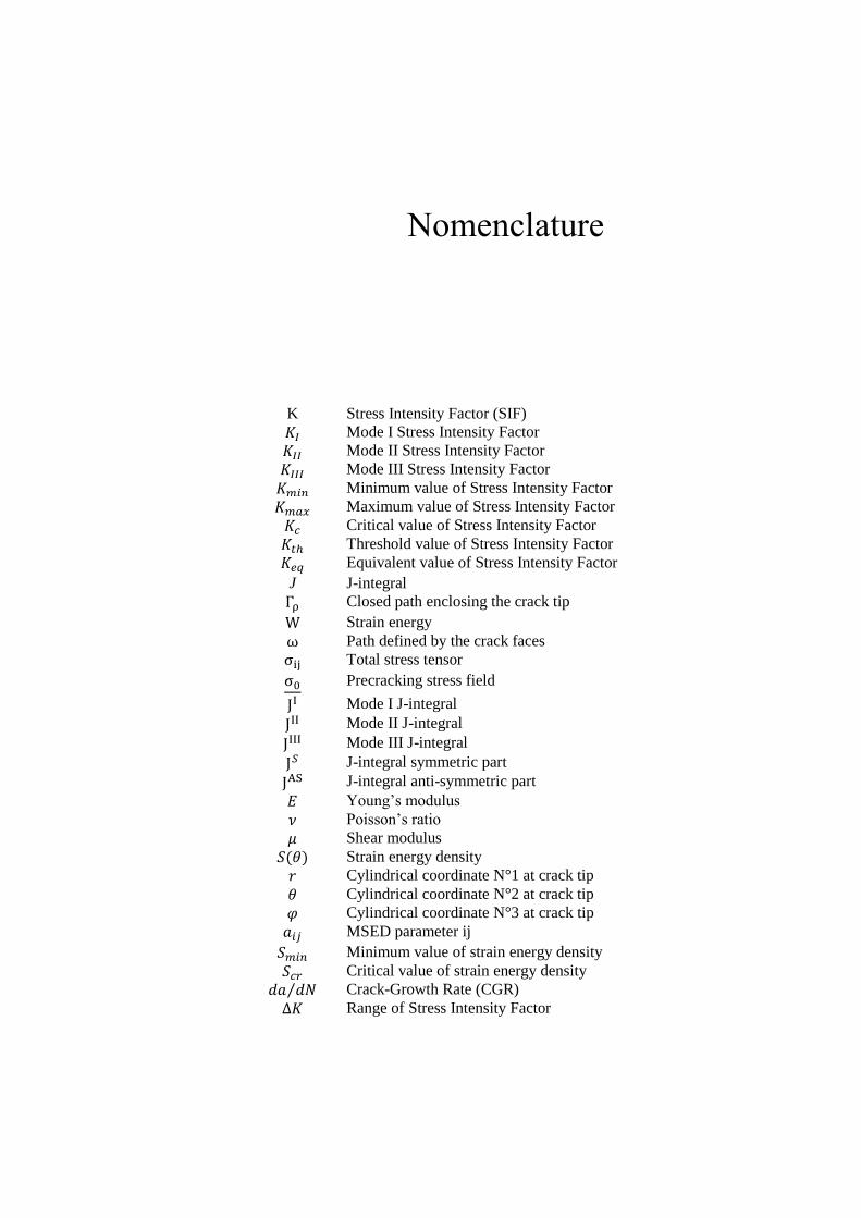
Nomenclature

K Stress Intensity Factor (SIF)

𝐾𝐼 Mode I Stress Intensity Factor

𝐾𝐼𝐼 Mode II Stress Intensity Factor

𝐾𝐼𝐼𝐼 Mode III Stress Intensity Factor

𝐾𝑚𝑖𝑛 Minimum value of Stress Intensity Factor

𝐾𝑚𝑎𝑥 Maximum value of Stress Intensity Factor

𝐾𝑐 Critical value of Stress Intensity Factor

𝐾𝑡ℎ Threshold value of Stress Intensity Factor

𝐾𝑒𝑞 Equivalent value of Stress Intensity Factor

J J-integral

Γρ Closed path enclosing the crack tip

W Strain energy

ω Path defined by the crack faces

σij Total stress tensor

σ0 Precracking stress field

JI Mode I J-integral

JII Mode II J-integral

JIII Mode III J-integral

J𝑆 J-integral symmetric part

JAS J-integral anti-symmetric part

𝐸 Young’s modulus

𝜈 Poisson’s ratio

𝜇 Shear modulus

𝑆(𝜃) Strain energy density

𝑟 Cylindrical coordinate N°1 at crack tip

𝜃 Cylindrical coordinate N°2 at crack tip

𝜑 Cylindrical coordinate N°3 at crack tip

𝑎𝑖𝑗 MSED parameter ij

𝑆𝑚𝑖𝑛 Minimum value of strain energy density

𝑆𝑐𝑟 Critical value of strain energy density

𝑑𝑎 𝑑𝑁⁄ Crack-Growth Rate (CGR)

∆𝐾 Range of Stress Intensity Factor

79

𝐶 Crack-growth law coefficient

𝑚 Crack-growth law exponent

𝑅 Stress ratio

𝑤 Walker law parameter

𝑓 NASGRO law parameter N° 1

𝑝 NASGRO law parameter N° 2

𝑞 NASGRO law parameter N° 3

𝑓𝑠 Static friction coefficient

𝛿 Shaft/hub interface clearance

𝑎 Crack dimension N° 1

𝑐 Crack dimension N° 2

𝐺𝑒𝑓𝑓 Effective value of energy release rate

α ZENCRACK parameter N° 1

𝐵 ZENCRACK parameter N° 2

𝑟 DBEM cut sphere radius

cfes Crack front element size

DOFs Degrees of freedom

α Thermal expansion coefficient