english translations of twenty-one of ertel’s papers on...
TRANSCRIPT

English translations of twenty-one of Ertel’s papers ongeophysical fluid dynamicsWAYNE SCHUBERT1∗, EBERHARD RUPRECHT2, ROLF HERTENSTEIN1, ROSANA NIETO FERREIRA3,RICHARD TAFT1, CHRISTOPHER ROZOFF1, PAUL CIESIELSKI1, HUNG-CHI KUO4
1Department of Atmospheric Science, Colorado State University, USA2Leibniz-Institut fur Meereswissenschaften an der Universitat Kiel3GEST Center, University of Maryland, USA4Department of Atmospheric Sciences, National Taiwan University, Taiwan
(Manuscript submitted January 20, 2004)
Abstract
This paper contains a collection of English translations of twenty-one of Hans Ertel’s papers on geophysicalfluid dynamics. The selected papers were originally published between 1942 and 1970 in either German orSpanish. This collection includes the four classic 1942 papers on vorticity and potential vorticity conservationprinciples and also papers on generalized conservation relations, hydrodynamic commutation formulas, Clebschand Weber transformations, and isogons and isotachs in two-dimensional flows.
Zusammenfassung
Dieser Artikel ist eine Sammlung von 21 Veroffentlichungen zur Stromungsdynamik von Hans Ertel. Die aus-gewahlten Artikel erschienen ursprunglich in deutscher oder spanischer Sprache im Zeitraum von 1942 bis 1970.In der Sammlung enthalten sind die vier klassischen Artikel von 1942 uber Vorticity und die Erhaltung poten-tieller Vorticity, sowie weitere Artikel zu allgemeinen Erhaltungssatzen, hydrodynamischen Vertauschungsrela-tionen, Clebsch- und Weber-Transformationen, und Isogonen und Isotachen in zweidimensiononalen Stromungen.
Preface
In view of the central role played by Ertel’s potentialvorticity in modern geophysical fluid dynamics, it mayseem surprising that few of our fellow scientists haveread Ertel’s original works on the subject. This may bebecause most of these original papers were not writtenin English and were published in journals not easily ac-cessible to many of us. It is in hopes of making Ertel’sworks more accessible that we provide the following setof translations.
The complete bibliography of Ertel’s scientific con-tributions, published between 1929 and 1972, lists astaggering 272 papers. Most of the papers are short,containing a concise mathematical argument and a briefphysical interpretation (figures are rare). The majorityof the papers are on meteorology, but there also appearpapers on oceanography, cosmology, atomic physics,volcanoes, fluvial erosion, etc. In selecting the papersfor this special issue we have limited the topic to geo-physical fluid dynamics and have been greatly aidedby the collection of original German and Spanish arti-cles reproduced in the five “Ertel volumes” edited by
W. Schroder and H.-J. Treder, published in coopera-tion with the Interdivisional Commission on Historyof the International Association of Geomagnetism andAeronomy (IAGA). The twenty-one translations pre-sented here are as follows:
1. ERTEL, H., 1942a: Ein neuer hydrodynamischerWirbelsatz. Meteorol. Z. (Braunschweig), 59(9), S.277–281.
2. ERTEL, H., 1942b: Ein neuer hydrodynamischerErhaltungssatz. Die Naturwiss. (Berlin), 30(36), S.543–544.
3. ERTEL, H., 1942c: Uber hydrodynamischeWirbelsatze. Physik. Z. (Leipzig), 43, S. 526–529.
4. ERTEL, H., 1942d: Uber das Verhaltnis des neuenhydrodynamischen Wirbelsatzes zum Zirkulationssatzvon V. Bjerknes. Meteorol. Z. (Braunschweig),59(12), S. 385–387.
5. ERTEL, H., 1952: Uber die physikalische Bedeutungvon Funktionen, welche in derClebsch-Transformation der hydrodynamischenGleichungen auftreten. Sitz.-Ber. Dt. Ak. d. Wiss.
∗Corresponding author: Wayne Schubert, Department of Atmospheric Science, Colorado State University, Fort Collins, Colorado, USA,80523, email: [email protected]
1

Berlin, Klasse f. Math. u. allg. Naturwiss., 1952, No.3, (Berlin 1952), S. 3–18.
6. ERTEL, H., 1955a: Kanonischer Algorithmushydrodynamischer Wirbelgleichungen. Sitz.-Ber. Dt.Ak. d. Wiss. Berlin, Klasse f. Math. u. allg.Naturwiss., 1954, No. 4, (Berlin 1955), S. 3–10.
7. ERTEL, H., 1955b: Ein neues Wirbel-Theorem derHydrodynamik. Sitz.-Ber. Dt. Ak. d. Wiss. Berlin,Klasse f. Math. u. allg. Naturwiss., 1954, No. 5,(Berlin 1955), S. 5–11.
8. ERTEL, H., 1956: Orthogonale Trajektoriensystemein stationaren ebenen Stromungsfelderninkompressibler idealer Flussigkeiten. Dt. Ak. d.Wissenschaften zu Berlin 1946–1956; Aus der Klassefur Mathematik, Physik und Technik, Berlin, S.67–71.
9. ERTEL, H., 1957: Sobre una relacion general entre lavelocidad del viento y la intensidad del campohidrodinamico en la atmosfera. Gerlands Beitr. z.Geophysik (Leipzig), 66(4), p. 323–329.
10. ERTEL, H., 1960a: Teorema sobre invariantessustanciales de la Hidrodinamica. Gerlands Beitr. z.Geophysik (Leipzig), 69(5), p. 290–293.
11. ERTEL, H., 1960b: Relacion entre la derivadaindividual y una cierta divergencia espacial enHidrodinamica. Gerlands Beitr. z. Geophysik(Leipzig), 69(6), p. 357–361.
12. ERTEL, H., 1961: Isoclinas e isotacas en corrientespotenciales bidimensionales de un fluidoincompresible. Gerlands Beitr. z. Geophysik(Leipzig), 70(1), p. 55–58.
13. ERTEL, H., 1963a: Analogıa entre las ecuaciones delmovimiento y las ecuaciones del torbellino en laHidrodinamica. Gerlands Beitr. z. Geophysik(Leipzig), 72(5), p. 312–314.
14. ERTEL, H., 1963b: Relaciones entre operacionesdiferenciales del calculo vectorial y parentesis deLagrange, con aplicacion a la Hydrodinamica.Geofisica pura e appl. (Milano), 55, 1963/II, p.119–122.
15. ERTEL, H., 1964: El numero maximo de invariantesindependientes en Hidrodinamica. Revista deGeofısica (Madrid), XXIII, Nums. 91/92, p. 121–124.
16. ERTEL, H., 1965a: HydrodynamischeVertauschungs-Relationen. Acta Hydrophysica,IX(3), Berlin, S. 115–123.
17. ERTEL, H., 1965b: Kommutative Operatoreninstationarer Stromungsfelder perfekter, piezotroperFlussigkeiten. Monatsber. Dt. Ak. d. Wiss. Berlin,7(4), S. 296–298.
18. ERTEL, H., 1965c: Theorem uber die unimodulareTransformation hydrodynamischerNumerierungskoordinaten. Gerlands Beitr. z.Geophysik (Leipzig), 74(3), S. 255–260.
19. ERTEL, H., 1970a: Eine Relation zwischenkinematischen Parametern horizontalerStromungsfelder in der Atmosphare. IdojarasBudapest, 74(1–2), S. 98–102.
20. ERTEL, H., 1970b: Spin und Deformationstensor imZusammenhand mit Isogonen und Isotachen inebenen Strommungsfeldern. Acta Geodaet., Geophys.et Montanist. Acad. Sci. Hung., Tomus 5 (3–4),Budapest, pp. 383–387.
21. ERTEL, H., 1970c: Transformation derDifferentialform der Weberschen hydrodynamischenGleichungen unter Berucksichtigung der Erdrotation.Gerlands Beitr. z. Geophysik (Leipzig), 79(6), p.421–424.
Some of these papers are best studied in groups.For example, papers 1–4 present the results on poten-tial vorticity with which we are so familiar. Whenthese four papers were published in 1942, many read-ers probably thought that the new potential vorticityequation was very elegant, but with practical applica-tions limited to tracer studies using special isentropicanalyses. Later developments, however, would provethat Ertel’s potential vorticity is much more useful thanthis simple initial understanding. The potential vortic-ity ρ−1(2Ω + ∇ × v) · ∇θ is a combination of thewind and mass fields. For general nonbalanced flows,knowledge of the potential vorticity field is not suffi-cient to determine both wind and mass. However, large-scale atmospheric flows are quasi-static, and the windand mass fields have mutually adjusted so that there ex-ists some kind of approximate balance between them(e.g., geostrophic, gradient, or nonlinear balance). Insuch situations, the density ρ, the velocity v, and thepotential temperature θ can all be expressed in terms ofthe pressure p, so that the potential vorticity determineseverything, if you can just invert it to find p. Thus, itis the concept of balance coupled with potential vor-ticity conservation which proves to be such a power-ful tool in analyzing geophysical flows. In addition,the transformation to different horizontal coordinates(e.g., geostrophic coordinates) or a different vertical co-ordinate (potential temperature) can often simplify themathematics and lead to concise and elegant descrip-tions of the dynamics. In any case, the fundamental un-derlying notion is Ertel’s potential vorticity (or an ap-propriate approximation to it); this is the motivation forour continuing interest in these classic 1942 papers.
2

Papers 6, 10, 11, and
22. ERTEL, H., and C.-G. ROSSBY, 1949: A newconservation theorem of hydrodynamics. GeofisicaPura e Appl. (Milano), 14, Fasc. 3–4, pp. 189–193.
can also be read as a group. The latter paper (22) is notincluded in the present collection since it was publishedin English (one of only two of Ertel’s papers that werepublished in English). This group of papers deals withgeneralizations of the original 1942 results. In particu-lar paper 6 provides a canonical algorithm from whichthe results of both the group 1–4 and paper 22 are easilyobtained.
Finally, papers 8, 12, 19, and 20 can also be readas a group. Reflecting Ertel’s interest in connecting dy-namic meteorology with operational practice in synop-tic meteorology, they deal with isogons and isotachs intwo-dimensional flow and the use of natural coordinatesystems.
In producing these translations we have attempted to
preserve the formatting of the original papers as muchas possible. References, for example, are cited in eachpaper with a style that matches that paper’s original for-matting, and the reference lists at the end of each paperare presented in their original untranslated forms. Cer-tain symbols and notations, however, were updated tomore modern conventions. For example, vector quan-tities have been represented using boldface symbols(rather than using an arrow symbol), and the “∇” sym-bol was used in place of the “grad” operator. Also, someformatting modifications were made in order to developsome coherency and consistency across the collectionof papers as a whole (such as the formatting of sectionheadings and equation numbers) and to deal with thetwo-column format of this journal (this affected the for-matting of many of the longer formulas). Although Er-tel’s papers are largely free of typographical errors in theequations, we did detect a few obvious ones, and thesehave been corrected in the translations.
1 ERTEL (1942a): A new hydrodynamical vorticity equation
Relative to a rotating coordinate system, whose ro-tation is given by the constant rotation vector Ω, one canwrite the Eulerian hydrodynamical equation for an idealcompressible fluid,
∂v
∂t+ ∇
(
12v2
)
− v × (∇× v) + 2Ω × v
= −∇Φ − α∇p,(1.1)
together with the continuity equation
dρ
dt=∂ρ
∂t+ v · ∇ρ = −ρ∇ · v. (1.2)
The foregoing symbols have the usual meaning (α =1/ρ is the specific volume, Φ the potential of externalforces).
The velocity ve is related to the position vector r
throughve = Ω × r. (1.3)
The velocity of a mass element relative to an inertialsystem (non-rotating system) then becomes
v + ve = v + Ω × r. (1.4)
Since∇× (Ω × r) = 2Ω, (1.5)
thenZ = ∇× (v + ve) = ∇× v + 2Ω, (1.6)
is the absolute vorticity, i.e., the vorticity relative to aninertial system, so that the Eulerian equation can bewritten
∂v
∂t+ ∇
(
12v2
)
− v × Z = −∇Φ − α∇p. (1.7)
Using
∇× (α∇p) = −∇p×∇α (1.8)
and taking the curl of (1.7), we obtain
∂
∂t∇× v −∇× (v × Z) = ∇p×∇α. (1.9)
Now consider ψ = ψ(r, t) to be a hydrodynamicalinvariant, i.e. a physical property which is conserved forevery fluid element:
dψ
dt=∂ψ
∂t+ v · ∇ψ = 0, (1.10)
as for example the potential temperature under adia-batic processes, or the polytropic temperature underpolytropic conditions1, or the total water content underconditions of no precipitation and without moisture in-put. In general, the invariant ψ does not have the same
3

value for all particles, but gives a field of ψ = constantsurfaces2.
Scalar multiplication of (1.9) by ∇ψ yields
∇ψ ·∂
∂t∇× v −∇ψ · ∇ × (v × Z)
= (∇p×∇α) · ∇ψ,(1.11)
or
∇ψ ·∂Z
∂t−∇ψ ·∇×(v×Z) = (∇p×∇α)·∇ψ, (1.12)
since from (1.6)
∂Z
∂t=
∂
∂t∇× v. (1.13)
Now, using
∇ · [∇ψ × (v × Z)] = −∇ψ · ∇ × (v × Z), (1.14)
(1.12) becomes
∇ψ·∂Z
∂t+∇·[∇ψ×(v×Z)] = (∇p×∇α)·∇ψ. (1.15)
The vector algebra formula (triple vector productformula)
a × (b × c) = b(c · a) − c(b · a) (1.16)
results in
∇ψ × (v × Z) = v(Z · ∇ψ) − Z(v · ∇ψ), (1.17)
which, along with
v · ∇ψ = −∂ψ
∂t,
allows us to write
∇ψ × (v × Z) = v(Z · ∇ψ) + Z∂ψ
∂t. (1.18)
Taking the divergence, we obtain
∇ · [∇ψ × (v × Z)] = v · ∇(Z · ∇ψ)
+ (Z · ∇ψ)∇ · v + Z ·∂
∂t∇ψ
(1.19)
since (1.5) and (1.6) imply
∇ · Z = 0. (1.20)
Substitution of (1.19) into (1.15) results in
∇ψ ·∂Z
∂t+ v · ∇(Z · ∇ψ) + Z ·
∂
∂t∇ψ
+ (Z · ∇ψ)∇ · v = (∇p×∇α) · ∇ψ(1.21)
which, because of
∇ψ ·∂Z
∂t+ Z ·
∂
∂t∇ψ =
∂
∂t(Z · ∇ψ) (1.22)
and
∂
∂t(Z · ∇ψ) + v · ∇(Z · ∇ψ) =
d
dt(Z · ∇ψ), (1.23)
gives
d
dt(Z·∇ψ)+(Z·∇ψ)∇·v = (∇p×∇α)·∇ψ. (1.24)
Division by ρ = 1/α and use of the equation
1
ρ∇ · v = −
1
ρ2
dρ
dt=
d
dt
(
1
ρ
)
=dα
dt(1.25)
results in
d
dt(αZ · ∇ψ) = α(∇p×∇α) · ∇ψ, (1.26)
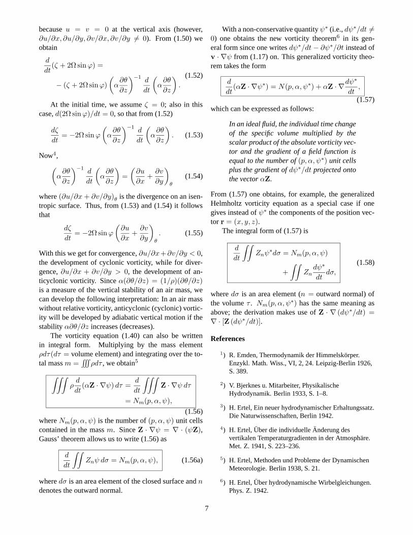
an equation whose right hand side has a very simplephysical meaning. To see this, consider the form
(∇α′ ×∇β′) · ∇γ′.
In so far as there is no homogeneous relationF (α′, β′) = 0 between the scalar functions α′ and β′,the surfaces α′(r, t) = constant and β ′(r, t) = constantform a solenoid system. If the third scalar function γ ′
is not of the form γ ′ = γ′(α′, β′), then this solenoid isdivided into cells between the surfaces γ ′(r, t) = con-stant. Assume all three families of surfaces are givenby
. . . , α′ − 1, α′, α′ + 1, . . .
. . . , β′ − 1, β′, β′ + 1, . . .
. . . , γ′ − 1, γ′, γ′ + 1, . . .
so that we have unit cells. Such a unit cell is shown inFig. 1.1. It is formed by the intersections of the surfaces
α′ = constant and α′ + 1 = constant
β′ = constant and β′ + 1 = constant
γ′ = constant and γ ′ + 1 = constant
The surface F in Fig. 1.1 is perpendicular to ∇α′ ×∇β′ and it contains the directions of the gradient ofα′ (which is the direction a) and of the gradient of β ′
(which is the direction b). The direction of c is that ofthe gradient of γ ′ which is perpendicular to the surfaceof constant γ′. The vector c and the normal of F formthe angle ν. The vectors a and b lie in the surface F and
4

Fig. 1.1
form the angle λ. This is also (except for higher orderterms) the angle between the surface α′ + 1 and the sur-face β′ (and between the surface α′ and the surface β′ +1), because a ⊥ α′ (a ⊥ α′ + 1) and b ⊥ β′ (b ⊥ β′ +1). The length of c is the height of the unit cell, becausec gives the distance between the surfaces of γ ′ +1 andγ′. The surface area of F is
F =ab
sinλ(1.27)
because a/ sinλ is the side of F to which b is perpen-dicular. Because the perpendicular to γ ′ and the perpen-dicular to F form the angle ν , the projection of F ontoγ′ is given by
projection of F =F
cos ν. (1.28)
The volume V of the unit cell is c(F/ cos ν), or
V =abc
sinλ cos ν. (1.29)
Now,
(∇α′ ×∇β′) · ∇γ′
= |∇α′||∇β′| sinλ|∇γ′| cos ν,(1.30)
and since
|∇α′| =(α′ + 1) − α′
a=
1
a
|∇β′| =(β′ + 1) − β′
b=
1
b
|∇γ′| =(γ′ + 1) − γ′
c=
1
c
, (1.31)
we have
(∇α′ ×∇β′) · ∇γ′ =sinλ cos ν
abc, (1.32)
which together with (1.29) gives
(∇α′ ×∇β′) · ∇γ′ =1
V, (1.33)
which is the inverse volume of an (α′, β′, γ′) unit cellor the number of (α′, β′, γ′) unit cells in a unit volume.Thus,
α(∇α′ ×∇β′) · ∇γ′ =α
V= N(α′, β′, γ′), (1.34)
the number of (α′, β′, γ′) unit cells in the specific vol-ume, i.e. in the volume occupied by a unit mass of fluid.Then,
α(∇p×∇α) · ∇ψ = N(p, α, ψ) (1.35)
5

the number of (p, α, ψ) unit cells in the specific volumeor the number of (p, α, ψ) unit cells per unit mass. Thesign of N(p, α, ψ) is positive if the vectors ∇p,∇α and∇ψ are cyclic; otherwise it is negative. Thus, we have
(∇p×∇α) · ∇ψ = (∇ψ ×∇p) · ∇α
= (∇α×∇ψ) · ∇p(1.36)
or
N(p, α, ψ) = N(ψ, p, α) = N(α, ψ, p), (1.37)
that is, the sign ofN(p, α, ψ) remains unchanged duringcyclic changes. Because of
a × b = −b × a, (1.38)
during non-cyclic changes, we have
N(p, α, ψ) = −N(p, ψ, α) = −N(ψ, α, p).
(1.39)Equation (1.26) can now be written as
d
dt(αZ · ∇ψ) =
d
dtα(∇× v + 2Ω) · ∇ψ
= N(p, α, ψ),
(1.40)which is the analytical form of the following vorticitytheorem:
The individual time change of the specificvolume multiplied by the scalar product ofthe absolute vorticity vector and the gradi-ent of a conservative property of every fluidparticle is equal to the number of (p, α, ψ)unit cells contained in the specific volumeα.
An important special case of the foregoing new vor-ticity theorem occurs when the conservative property ψcan be written as a function of p and α,
ψ = ψ(p, α), (1.41)
for example, in the case when ψ is the polytropic tem-perature (see R. Emden). Then we have
∇ψ =∂ψ
∂p∇p+
∂ψ
∂α∇α, (1.42)
and, as a consequence,
N(p, α, ψ) = α∂ψ
∂p(∇p×∇α) · ∇p
+ α∂ψ
∂α(∇p×∇α) · ∇α
= 0
(1.43)
and
(∇p×∇α) · ∇p = (∇p×∇α) · ∇α = 0. (1.44)
The volume V of a (p, α, ψ) unit cell becomes infi-nite and the cells degenerate into solenoids; the (p, α)solenoid, the (p, ψ) solenoid, and the (ψ, α) solenoidhave the same direction at each point, a direction which,however, can be different for different points.
The vorticity theorem (1.40) then becomes a hydro-dynamical conservation theorem
d
dtα(∇× v + 2Ω) · ∇ψ = 0, (1.45)
the derivation of which I have recently given in anotherway3. The adiabatic motion in the atmosphere (as a spe-cial case of the polytropic case) satisfies
d
dtα(∇× v + 2Ω) · ∇θ = 0. (1.46)
Here,
θ = T
(
1000
p
)κ
=1000κ
Rp1−κα (1.47)
is the potential temperature (R = gas constant, κ =R/cp). The adiabatic special case of the new vorticitytheorem, that is (1.46), may prove to be a very usefultool for isentropic analysis (C. G. Rossby).
Here let us discuss as an application of (1.46), thebeginning of an adiabatic vertical motion along the ver-tical axis of expansion or contraction of a volume ofair. If the positive z axis is upward and if (x, y, z) isa right-hand cartesian system, the horizontal (x, y) sur-face touches the earth’s surface at latitude ϕ and
k · ∇ × v =∂v
∂x−∂u
∂y= ζ (1.48)
(ζ > 0 for cyclonic motion and ζ < 0 for anticyclonicmotion) and
k · Ω = Ω sinϕ > 0 (for the northern
hemisphere).(1.49)
The conservation theorem (1.46) gives
d
dt
α(ζ + 2Ω sinϕ)∂θ
∂z
= 0, (1.50)
whered
dt=
∂
∂t+ w
∂
∂z(1.51)
6
because u = v = 0 at the vertical axis (however,∂u/∂x, ∂u/∂y, ∂v/∂x, ∂v/∂y 6= 0). From (1.50) weobtain
d
dt(ζ + 2Ω sinϕ) =
− (ζ + 2Ω sinϕ)
(
α∂θ
∂z
)
−1 d
dt
(
α∂θ
∂z
)
.
(1.52)
At the initial time, we assume ζ = 0; also in thiscase, d(2Ω sinϕ)/dt = 0, so that from (1.52)
dζ
dt= −2Ω sinϕ
(
α∂θ
∂z
)
−1 d
dt
(
α∂θ
∂z
)
. (1.53)
Now4,(
α∂θ
∂z
)
−1 d
dt
(
α∂θ
∂z
)
=
(
∂u
∂x+∂v
∂y
)
θ
(1.54)
where (∂u/∂x+ ∂v/∂y)θ is the divergence on an isen-tropic surface. Thus, from (1.53) and (1.54) it followsthat
dζ
dt= −2Ω sinϕ
(
∂u
∂x+∂v
∂y
)
θ
. (1.55)
With this we get for convergence, ∂u/∂x+∂v/∂y < 0,the development of cyclonic vorticity, while for diver-gence, ∂u/∂x + ∂v/∂y > 0, the development of an-ticyclonic vorticity. Since α(∂θ/∂z) = (1/ρ)(∂θ/∂z)is a measure of the vertical stability of an air mass, wecan develop the following interpretation: In an air masswithout relative vorticity, anticyclonic (cyclonic) vortic-ity will be developed by adiabatic vertical motion if thestability α∂θ/∂z increases (decreases).
The vorticity equation (1.40) can also be writtenin integral form. Multiplying by the mass elementρdτ(dτ = volume element) and integrating over the to-tal mass m =
∫∫∫
ρdτ , we obtain5
∫∫∫
ρd
dt(αZ · ∇ψ) dτ =
d
dt
∫∫∫
Z · ∇ψ dτ
= Nm(p, α, ψ),
(1.56)where Nm(p, α, ψ) is the number of (p, α, ψ) unit cellscontained in the mass m. Since Z · ∇ψ = ∇ · (ψZ),Gauss’ theorem allows us to write (1.56) as
d
dt
∫∫
Znψ dσ = Nm(p, α, ψ), (1.56a)
where dσ is an area element of the closed surface and ndenotes the outward normal.
With a non-conservative quantityψ∗ (i.e., dψ∗/dt 6=0) one obtains the new vorticity theorem6 in its gen-eral form since one writes dψ∗/dt− ∂ψ∗/∂t instead ofv · ∇ψ from (1.17) on. This generalized vorticity theo-rem takes the form
d
dt(αZ · ∇ψ∗) = N(p, α, ψ∗) + αZ · ∇
dψ∗
dt,
(1.57)which can be expressed as follows:
In an ideal fluid, the individual time changeof the specific volume multiplied by thescalar product of the absolute vorticity vec-tor and the gradient of a field function isequal to the number of (p, α, ψ∗) unit cellsplus the gradient of dψ∗/dt projected ontothe vector αZ.
From (1.57) one obtains, for example, the generalizedHelmholtz vorticity equation as a special case if onegives instead of ψ∗ the components of the position vec-tor r = (x, y, z).
The integral form of (1.57) is
d
dt
∫∫
Znψ∗dσ = Nm(p, α, ψ)
+
∫∫
Zndψ∗
dtdσ,
(1.58)
where dσ is an area element (n = outward normal) ofthe volume τ . Nm(p, α, ψ∗) has the same meaning asabove; the derivation makes use of Z · ∇ (dψ∗/dt) =∇ · [Z (dψ∗/dt)].
References
1) R. Emden, Thermodynamik der Himmelskorper.Enzykl. Math. Wiss., VI, 2, 24. Leipzig-Berlin 1926,S. 389.
2) V. Bjerknes u. Mitarbeiter, PhysikalischeHydrodynamik. Berlin 1933, S. 1–8.
3) H. Ertel, Ein neuer hydrodynamischer Erhaltungssatz.Die Naturwissenschaften, Berlin 1942.
4) H. Ertel, Uber die individuelle Anderung desvertikalen Temperaturgradienten in der Atmosphare.Met. Z. 1941, S. 223–236.
5) H. Ertel, Methoden und Probleme der DynamischenMeteorologie. Berlin 1938, S. 21.
6) H. Ertel, Uber hydrodynamische Wirbelgleichungen.Phys. Z. 1942.
7

2 ERTEL (1942b): A new hydrodynamical conservation principle
In a compressible fluid whose particles move poly-tropically, the specific volume α can be expressed as afunction of the pressure p and the “polytropic temper-ature” Θs = T (ρ0/ρ)
1/s (s = (cv − β) / (cp − cv) isthe polytropic order, β = dQ/dT the constant poly-tropic specific heat capacity, ρ = 1/α the density, andρ0 = 1 g/cm3)1:
α =1
ρ= ψ(p,Θs). (2.1)
In general, Θs varies from particle to particle butremains constant in time for a given particle:
dΘs
dt=∂Θs
∂t+ v · ∇Θs =
∂Θs
∂t+ vk
∂Θs
∂xk= 0, (2.2)
the last part of which makes use of the usual summa-tion convention. With respect to a rotating rectangularcartesian coordinate system (xi, i = 1, 2, 3) whose ro-tation is described by the constant rotation vector Ω, thehydrodynamical vorticity equation2 can be written
d
dt
(
ξiρ
)
−
(
ξkρ
)
∂vi∂xk
= −1
ρ∇×
(
1
ρ∇p
)
, (2.3)
whereξ = ∇× v + 2Ω (2.4)
denotes the absolute (relative to an inertial system) vor-ticity vector and where v = vi (i = 1, 2, 3) denotes thewind relative to the rotating xi system.
On account of (2.1),
∇×
(
1
ρ∇p
)
=∂ψ
∂Θs∇Θs ×∇p
or in component form
[
∇×
(
1
ρ∇p
)]
i
=∂ψ
∂Θsεijk
∂Θs
∂xj
∂p
∂xk,
where εijk denotes the following tensor:
εijk =
1 for a cyclic sequence of indices−1 for a non-cyclic sequence of indices
0 if any two indices agree
The vorticity equation (2.3) can now be written (ξ =ξi, i = 1, 2, 3)
d
dt(αξi) − (αξk)
∂vi∂xk
= −α∂ψ
∂Θsεijk
∂Θs
∂xj
∂p
∂xk. (2.5)
Multiplying by ∂Θs/∂xr and making use of
εijk∂Θs
∂xi
∂Θs
∂xj
∂p
∂xk= 0,
it follows from (2.5) that
∂Θs
∂xi
d
dt(αξi) − (αξk)
∂vi∂xk
∂Θs
∂xi= 0, (2.6)
or in another form
d
dt
(
α∂Θs
∂xiξi
)
− (αξi)d
dt
(
∂Θs
∂xi
)
− (αξk)∂vi∂xk
∂Θs
∂xi= 0.
(2.7)
From (2.2) we now obtain
∂
∂xi
(
dΘs
dt
)
=d
dt
(
∂Θs
∂xi
)
+∂Θs
∂xk
∂vk∂xi
= 0, (2.8)
so that
ξid
dt
(
∂Θs
∂xi
)
= −ξi∂Θs
∂xk
∂vk∂xi
= −ξk∂Θs
∂xi
∂vi∂xk
, (2.9)
and the substitution of (2.9) into (2.7) leads to the fol-lowing conservation principle:
d
dt
(
αξi∂Θs
∂xi
)
=d
dtα (∇× v + 2Ω)n∇nΘs
= 0,
(2.10)where n denotes the direction normal to the planes ofconstant polytropic temperature and toward increasingΘs. Equation (2.10) is the analytical version of the fol-lowing conservation principle3:
In a fluid which moves polytropically, thequantity formed by multiplying the specificvolume by the scalar product of the abso-lute vorticity vector and the gradient of thepolytropic temperature is conserved follow-ing individual particles.
For s = cv/(cp − cv), the polytropic temperaturereduces to the potential temperature
θ = T
(
P
p
)κ
(2.11)
(P = reference pressure, e.g. 1000 mb, and κ = R/cp)and (2.2) becomes
dθ
dt= 0.
8

The conservation principle then becomes
d
dtα (∇× v + 2Ω)n∇nθ = 0, (2.12)
which in meteorology is connected to the isentropicanalysis work of C. G. Rossby.
References
1) R. EMDEN, Thermodynamik der Himmelskorper.
Enzykl. Math. Wiss., VI, 2, 24, S. 389.Berlin-Leipzig 1926.
2) W. VOIGT, Kompendium der theoretischen Physik I,270.–Leipzig 1895.
3) The conservation principle given here can be regardedas a special case of the new hydrodynamical vorticityequation which I have proven in another paper.(Meteorol. Z. 1942).
3 ERTEL (1942c): On hydrodynamical vorticity equations
I. Introduction
Adopting the usual summation convention (accord-ing to which every index occurring twice in a single termis summed from 1 to 3) the vorticity equation for anideal compressible fluid reads as follows:
d
dt(αζi) − (αζk)
∂wi∂zk
= εijkα∂p
∂zj
∂α
∂zk, (3.1)
where α = ρ−1 is the specific volume, p the pressure,zi(i = 1, 2, 3) the rectangular cartesian (inertial) coor-dinate system, wi(i = 1, 2, 3) the wind components,ζi = εijk (∂wk/∂zj) = (∇× w)i, and
εijk =
1 for a cyclic sequence of indices,−1 for a non-cyclic sequence of indices,
0 if any two indices agree.
Through a generalization of (3.1) we shall now derive anew vorticity equation.
II. General formulation of hydrodynamical vorticityequations by means of a commutator relation
In order to treat the most general case we refer notto the inertial system as in (3.1) but rather to a rotatingrectangular coordinate system xi, whose rotation is de-scribed by the constant rotation vector fi(i = 1, 2, 3);the vorticity equations then take the form
d
dt(αξi) − (αξk)
∂vi∂xk
= εijkα∂p
∂xj
∂α
∂xk(3.2)
with the individual (material) derivative operator
d
dt=
∂
∂t+ vk
∂
∂xk(3.3)
and the absolute vorticity
ξi = εijk∂vk∂xj
+ 2fi , (3.4)
in which vi(i = 1, 2, 3) is the wind component andεijk (∂vk/∂xj) is the vorticity relative to the rotating xi-system. The existence of a potential for other forces isimplicit in (3.2).
Scalar multiplication of (3.2) by the gradient∂ψ/∂xi of a hydrodynamical field function ψ (scalar,vector or tensor component) leads easily to the form
d
dt
(
αξi∂ψ
∂xi
)
− (αξi)d
dt
(
∂ψ
∂xi
)
− (αξk)∂ψ
∂xi
∂vi∂xk
= αεijk∂ψ
∂xi
∂p
∂xj
∂α
∂xk,
which, through the exchange of the summation indicesin the third term on the left side, can be written
d
dt
(
αξi∂ψ
∂xi
)
− (αξi)
d
dt
(
∂ψ
∂xi
)
+∂ψ
∂xk
∂vk∂xi
= αεijk∂ψ
∂xi
∂p
∂xj
∂α
∂xk.
(3.5)
Now, from (3.3), we have
d
dt
(
∂ψ
∂xi
)
=∂2ψ
∂xi∂t+ vk
∂2ψ
∂xi∂xk
=∂
∂xi
(
dψ
dt
)
−∂ψ
∂xk
∂vk∂xi
,
with which (3.5) can be reduced to
d
dt
(
αξi∂ψ
∂xi
)
−
(
αξi∂
∂xi
)
dψ
dt
= αεijk∂ψ
∂xi
∂p
∂xj
∂α
∂xk,
(3.6)
9

whose right hand side has the following simple mean-ing: Assume that the surfaces p = const, α = const andψ = const (with scalar value differences of 1) are con-structed throughout space; each set of surfaces dividesspace into unit layers. As long as there is no homoge-neous relation F (p, α) = 0 (V. Bjerknes1) between pand α, the intersections of the p and α unit layers form(p, α) unit solenoids. The (p, α) unit solenoids are in-tersected by the ψ unit layers, as long as ψ is not of theform ψ = ψ (p, α). In this way a field of (p, α, ψ) unitcells is formed. We can then interpret
εijk∂ψ
∂xi
∂p
∂xj
∂α
∂xk= (∇p×∇α) · ∇ψ = ±
1
V(3.7)
as the reciprocal volume V of a (p, α, ψ) unit cell orthe number of (p, α, ψ) unit cells in a unit volume. Theproof is accomplished by integration of (∇p × ∇α) ·∇ψ = ∇ · (ψ∇p ×∇α) over the volume of a unit celland application of Gauss’ integral theorem; the portionof the surface integral over the four sides of the (p, α)solenoids disappears, and the remainder yields a valueof +1 or −1, depending on whether the three gradients∇p,∇α,∇ψ are oriented in the sense of a right-handedor left-handed screw. (For a related discussion see H.Ertel2). Thus, we can interpret
αεijk∂ψ
∂xi
∂p
∂xj
∂α
∂xk= α (∇p×∇α) · ∇ψ
= ±α
V= N (p, α, ψ)
(3.8)
as the (positive or negative) number N(p, α, ψ) of(p, α, ψ) unit cells in the specific volume; moreover itfollows from (3.7) that
N(p, α, ψ) = N(ψ, p, α) = N(α, ψ, p)
N(p, α, ψ) = −N(α, p, ψ) = −N(ψ, α, p)
. (3.9)
Furthermore N(p, α, ψ) = 0 for homogeneous fluids(∇ρ = 0) while for inhomogeneous fluids (∇ρ 6= 0)
N(p, α, ψ) = 0, if
ψ = ψ(p)
ψ = ψ(α)
ψ = ψ(p, α)
α = α(p)
. (3.10)
Combining (3.6) and (3.8) we obtain
d
dt
(
αξi∂ψ
∂xi
)
−
(
αξi∂
∂xi
)
dψ
dt= N (p, α, ψ) ,
(3.11)
a generalized formulation for hydrodynamical vorticityequations in the commutator relation form
(D1D2 −D2D1)ψ = N (p, α, ψ) , (3.12)
where the operators
D1 =d
dt=
∂
∂t+ vk
∂
∂xk=
∂
∂t+ (v · ∇) (3.13)
and
D2 = αξi∂
∂xi= αξk
∂
∂xk= α (∇× v + 2f) · ∇
(3.14)are in general not commutative.
Multiplying (3.11) by the mass element ρdτ (dτ =volume element), integrating over the volume τ contain-ing the total mass m =
∫∫∫
ρdτ , using αρ = 1, andnoting that
∫∫∫
ρd
dt
(
αξi∂ψ
∂xi
)
dτ =D
Dt
∫∫∫
ξi∂ψ
∂xidτ
=D
Dt
∫∫∫
∂ (ψξi)
∂xidτ
=D
Dt
∫∫
ψξndΩ,
(3.15)
as well as∫∫∫
ξi∂
∂xi
(
dψ
dt
)
dτ =
∫∫∫
∂
∂xi
(
ξidψ
dt
)
dτ
=
∫∫
ξndψ
dtdΩ,
(3.16)
yields in the integral form (dΩ = surface element of τ ;n = outward normal)
D
Dt
∫∫
ξnψ dΩ −
∫∫
ξndψ
dtdΩ = Nm (p, α, ψ) ,
(3.17)where Nm (p, α, ψ) =
∫∫∫
ρN (p, α, ψ) dτ is the num-ber of (p, α, ψ) unit cells contained in the total mass mand D
Dt denotes the individual time derivative of the en-tire moving mass; in this derivation we note that for anyF (F = scalar, vector- or tensor-component) we have
D
Dt
∫∫∫
ρFdτ =
∫∫∫
∂ (ρF )
∂tdτ +
∫∫
ρvnFdΩ
=
∫∫∫
ρdF
dtdτ ,
(3.18)
since, by means of the continuity equation
∂ρ
∂t+ ∇ · (ρv) = 0 (3.19)
10

the following transformation is possible:∫∫∫
∂ (ρF )
∂tdτ +
∫∫
ρvnFdΩ
=
∫∫∫
∂(ρF )
∂t+ ∇ · (ρvF )
dτ
=
∫∫∫
ρ
∂F
∂t+ (v · ∇)F
dτ.
Equation (3.18) with F = αξi (∂ψ/∂xi) revertsback to (3.15) when we take into consideration the factthat ξi represents a nondivergent vector, i.e.
∂ξi∂xi
= 0. (3.20)
III. Conclusions
A. If one substitutes for ψ in (3.11) or (3.12) the compo-nents xs (s = 1, 2, 3) of the position vector r of a fluidparticle, one obtains, because D1xs = vs, the vorticityequation (3.2), which for a homogeneous and incom-pressible fluid, turns into the Helmholtz vorticity equa-tion in the rotating system.
B. If ψ is a conservative property of a fluid particle,
D1ψ =dψ
dt= 0, (3.21)
and it then follows from (3.11) or (3.12) that
d
dt
(
αξi∂ψ
∂xi
)
= N (p, α, ψ) , (3.22)
which can be stated as follows:
For a fluid variable ψ which is individu-ally conserved but has spatial variability,the individual time change of the specificvolume multiplied by the scalar product ofthe absolute vorticity vector with the gradi-ent of ψ is equal to the number of (p, α, ψ)unit cells contained in the specific volumeα.
C. If ψ is a conserved quantity and at the same time hasthe form
ψ = ψ (p, α) , (3.23)
for all fluid particles, then, because
∇ψ =∂ψ
∂p∇p+
∂ψ
∂α∇α,
(3.10) yields N (p, α, ψ) = 0 and (3.22) reduces to
d
dt
(
αξi∂ψ
∂xi
)
= 0, (3.24)
which is an analytical statement of the following con-servation principle:
For a fluid variable ψ which is individuallyconserved but has a spatial variability suchthat it depends only on pressure and spe-cific volume, the individual time change ofthe specific volume multiplied by the scalarproduct of the absolute vorticity vector withthe gradient of ψ vanishes.
An example of a function ψ which satisfies condi-tions (3.21) and (3.23) is the entropy of an ideal gaswhich moves adiabatically; another example is the poly-tropic temperature3 of an ideal gas which moves poly-tropically; the conservation principle is therefore validfor adiabatic or polytropic currents in ideal gases withspatially variable entropy or polytropic temperature (theearth’s atmosphere, stellar atmospheres).
D. A homogeneous fluid is defined by ∇α = ∇ (1/ρ) =0, from which (using (3.8)) it follows that N (p.α, ψ)vanishes for any function ψ; furthermore, N (p, α, ψ)vanishes for any function ψ in the case of barotropy, i.e.α = α (p). Then, there follows from (3.12) the princi-ple:
For homogeneous fluids and for inhomoge-neous barotropic fluids the operators D1
and D2 are always commutative; on theother hand, for inhomogeneous baroclinicfluids, the operators D1 and D2 are onlycommutative for those functions ψ whichcause the determinant
∂ (p, α, ψ)
∂ (x1, x2, x3)= (∇p×∇α) · ∇ψ
to vanish.
References
1) V. Bjerknes und Mitarbeiter, PhysikalischeHydrodynamik, S. 3ff., Berlin 1933.
2) H. Ertel, Meteorol. Zeitschr., 59, 1942.
3) R. Emden, Enzykl. Math. Wiss., VI, 2, 24, Leipzigund Berlin 1926.
11

4 ERTEL (1942d): On the relationship between the new hydrodynamic vorticitytheorem and Bjerknes’ circulation theorem
Summary
It is proven that Bjerknes’ circulation theorem is a specialcase of the new hydrodynamical vorticity theorem.
1. The new vorticity theorem
Recently I derived a very general hydrodynamicvorticity theorem [1] [2]. In its differential form it readsas follows:
d
dt(σW · ∇ψ) − (σW · ∇)
dψ
dt= N(p, σ, ψ).
(4.1)It has the form of a commutation relation
(D1D2 −D2D1)ψ = N(p, σ, ψ) (4.2)
with the generally noncommutative operators
D1 =d
dt=
∂
∂t+ v · ∇ (4.3)
and
D2 = (σW · ∇) = σ(rotv + 2f) · ∇, (4.4)
where the symbols used in (4.1) through (4.4) are de-fined as follows: σ = specific volume = 1/ρ ( ρ =density); p = pressure; v = velocity vector relativeto a coordinate system, its rotation described throughthe constant rotation vector f ; W = rotv + 2 f =(absolute) vorticity; ψ = hydrodynamic field function(scalar, vector, or tensor component); N(p, σ, ψ) =σ[∇p,∇σ] · ∇ψ = number of (p, σ, ψ)-cells containedwithin a specific volume σ.
For the derivation of (4.1), it has been assumed thatthe fluid is ideal and that external forces acting on thefluid possess a potential. The sign of N(p, σ, ψ) is pos-itive or negative depending on whether the generallynonorthogonal vectors ∇p, ∇σ and ∇ψ are oriented ina right- or left-handed system.
One can obtain equations for each component ofvorticity by specifying in (4.1) the function ψ to havea purely geometric interpretation. Namely, one succes-sively sets ψ = x, ψ = y, and ψ = z in such a way thatfrom (4.1) the following vorticity equations result:
d
dt(σWx) − (σW · ∇)vx = σ[∇p,∇σ]x,
d
dt(σWy) − (σW · ∇)vy = σ[∇p,∇σ]y,
d
dt(σWz) − (σW · ∇)vz = σ[∇p,∇σ]z,
(4.5)
where, for instance,
[∇p,∇σ]x =∂p
∂y
∂σ
∂z−∂p
∂z
∂σ
∂y(4.6)
is the number of the isobar-isostere unit solenoids perunit surface area normal to the +x direction. For ir-rotational coordinates (f ≡ 0) and barotropy (p =p(σ)), (4.5) yields the vorticity equations of E. J.NANSON (1874); furthermore, adding incompressibil-ity, one obtains the vorticity equations of HELMHOLTZ
(1858) [LAGRANGE (1781), CAUCHY (1827), STOKES
(1848)].The integral form of the new vorticity theorem reads
(Ertel, l.c.):
d
dt
∫∫
WnψdΩ −
∫∫
Wndψ
dtdΩ = Nm(p, σ, ψ).
(4.7)Here,
Nm(p, σ, ψ) =
∫∫∫
ρN(p, σ, ψ)dτ
=
∫∫∫
[∇p,∇σ] · ∇ψdτ
(4.8)
is the number of (p, σ, ψ)-unit cells, m =∫∫∫
ρdτ is themass (with volume τ contained in the surface Ω), and nin (4.7) represents the outward normal. Because
[∇p,∇σ] · ∇ψ = ∇ · (ψ[∇p,∇σ]),
(4.8) can be transformed through Gauss’ integral theo-rem into
Nm(p, σ, ψ) =
∫∫
ψ[∇p,∇σ]ndΩ. (4.9)
Then, the integral form (4.7) of the new vorticity theo-rem changes into
d
dt
∫∫
WnψdΩ −
∫∫
Wndψ
dtdΩ
=
∫∫
ψ[∇p,∇σ]ndΩ.
(4.10)
One assumes in (4.7) and (4.10) that the functions ψ,dψ/dt, W and [∇p,∇σ] are defined on the surface Ωand in the volume τ the first derivatives are continuous
12

with respect to the spatial coordinates; the closed sur-face Ω can itself consist of finitely many pieces of con-tinuous tangential planes.
2. The new vorticity theorem with a discontinuousψ-function
Consider discontinuous ψ and dψ/dt on the surfaceΣ. We denote the jump in ψ as
ψ = ψ+0 − ψ−0 (4.11)
and the jump in dψ/dt as
dψ
dt
=
(
dψ
dt
)
+0
−
(
dψ
dt
)
−0
(4.12)
on the surface Σ (the indices +0 and −0 specify thefunction values directly above and directly below thesurface Σ, respectively). Then, we construct a cylin-der with face F parallel to Σ and the infinitesmal heighth. Applying the integral form (4.10) of the new vortic-ity theorem to the region F · h and taking the limit ash→ 0, the integral over the lateral surface vanishes andwe obtain the following:
d
dt
∫∫
Wnψ−0dF −
∫∫
Wn
(
dψ
dt
)
+0
dF
+d
dt
∫∫
W−nψ−0dF −
∫∫
W−n
(
dψ
dt
)
−0
dF
=
∫∫
ψ+0[∇p,∇σ]ndF
+
∫∫
ψ−0[∇p,∇σ]−ndF (4.13)
By the continuity of W and [∇p,∇σ] on Σ (and thuson the subarea F of Σ)
W−n = −Wn
and[∇p,∇σ]−n = [∇p,∇σ]n.
Then, in consideration of (4.11) and (4.12) we can write
d
dt
∫∫
Wn ψ dF −
∫∫
Wn
dψ
dt
dF
=
∫∫
ψ [∇p,∇σ]ndF.
(4.14)Equation (4.14) represents the integral form of the newvorticity theorem for a field function ψ and discontinu-ous derivative dψ/dt on the surface F .
If, on the surface F , only the field function ψ be-comes discontinuous;
ψ = ψ+0 − ψ−0 6= 0,
while dψ/dt, however, remains continuous:
dψ
dt
=
(
dψ
dt
)
+0
−
(
dψ
dt
)
−0
= 0,
then (4.14) reduces to
d
dt
∫∫
ψWndF =
∫∫
ψ [∇p,∇σ]ndF.
(4.15)By properly specifying the function ψ, Bjerknes’ circu-lation theorem results from equation (4.15).
3. The circulation theorem of V. Bjerknes as a specialcase of the new vorticity theorem
The surface Σ, which contains the surface F , di-vides the fluid into an “upper fluid half-space” R 1 and a“lower fluid half-space” R 2. The surface Σ, and with itF , moves with the current, such that particles which arein R1 always remain in R1 and particles in R2 alwaysremain in R2, while the common boundary Σ (with thesurface F ) of the two fluid spaces R 1 and R2 deformsitself according to the flow. We now imagine that eachfluid particle in R 1 is assigned a same constant numberZ1; thus, this number identifies each individual fluid ele-ment belonging to the fluid half-spaceR 1. Similarly, weimagine all fluid particles from R 2 possessing the sameconstant number Z2. The numbers Z1 and Z2 do notcharacterize the fluid particles individually, because, forinstance, all fluid particles in R 1 are assigned the samenumber Z1; rather, the numbers Z1 and Z2 are groupdistinguisher indices that decide which of the two ap-plicable groups of fluid particles each particle belongsto. However, each fluid element maintains the assignednumber of Z1 or Z2 individually:
d
dtZ1 =
d
dtZ2 = 0.
For example, a particle initially assigned a numberZ1 and belonging to the fluid half-space R 1 cannot be-long to R2 later and not have the assigned number Z2
with it, since the particle would have to cross the sur-face Σ. This is impossible since the same number is al-ways associated with the same particle, if Σ, as adopted,moves along with the flow. However, the number (ei-ther Z1 or Z2) changes discontinuously at the surfacesΣ and F as |Z1 − Z2| 6= 0. The restriction of a fluidelement to either the fluid half-space R 1 or to the fluidhalf-space R2 with these two characteristic numbers Z1
13

Fig. 4.1
and Z2 thus forms a discontinuous ψ-field with the char-acteristics
ψ = Z1,dψ
dt= 0 (in R1),
ψ = Z2,dψ
dt= 0 (in R2),
as well as
ψ = ψ+0 − ψ−0
= Z1 − Z2 6= 0 (on Σ and/or F )(4.16)
and
dψ
dt
=
(
dψ
dt
)
+0
−
(
dψ
dt
)
−0
= 0, (on Σ and/or F )
(4.17)
where for this ψ-function the new vorticity theorem ofthe form (4.15) applies. Since ψ = Z1 − Z2 is aconstant jump value on Σ and/or F , the equation (4.15)immediately results in
(Z1 − Z2)d
dt
∫∫
WndF
= (Z1 − Z2)
∫∫
[∇p,∇σ]ndF,
or through division by Z1 − Z2 6= 0,
d
dt
∫∫
WndF =
∫∫
[∇p,∇σ]ndF, (4.18)
which is the equation that represents Bjerknes’ circula-tion theorem.
We note that∫∫
[∇p,∇σ]ndF = N(p, σ) (4.19)
is the quantity of isobar-isostere unit solenoids in F and∫∫
WndF =
∫∫
(rotnv + 2fn)dF
=
∮
vsds+ 2ωS
(4.20)
is the absolute circulation along the boundary of F .Then, through Stokes’ theorem,
∫∫
rotnv dF =
∮
vs ds = C
is the circulation C relative to the Earth (rotating sys-tem). Furthermore,
2
∫∫
fndF = 2
∫∫
ω cos(n, f)dF
= 2ωS
is twice the angular velocity ω = |f | multiplied by theprojection S =
∫∫
cos(n, f)dF of the area F onto anyplane (e.g., equatorial plane) perpendicular to the rota-tion axis, and thus (4.18) is equivalent with the usualversion of the Bjerknes’ circulation theorem:
dC
dt+ 2ω
dS
dt= N(p, σ). (4.21)
Following (4.15) one obtains Lord Kelvin’s circula-tion theorem for irrotational coordinates (f = 0) and abarotropic fluid (p = p(σ)) [W. THOMSON (1869)]:
d
dt
∮
vsds = 0. (4.22)
In summary, from the new hydrodynamic vorticitytheorem in its differential and integral forms, all well-known vorticity and circulation equations, respectively,can be derived as special cases. In addition, the newvorticity theorem results in still unknown special cases,for example, a conservation law valid for polytropicflows [3] (ψ = polytropic temperature), for which F.MORAN [4] has furnished a very appealing proof.
References1] H. Ertel, Met. Z. 1942.
2] H. Ertel, Physik. Z. 1942.
3] H. Ertel, Die Naturwissenschaften 1942.
4] F. Moran, Revista de Geofisica 1942.
14

5 ERTEL (1952): On the physical significance of functions arising in the Clebschtransformation of the hydrodynamical equations
I. Geometry and kinematics of a stationarybarotropic fluid
In the Clebsch transformation of the hydrodynamicequations [Ref. (1, 2, 3)] the wind velocity vector v isrepresented by the superposition of two vectors [Ref.(4)] involving the three scalar functions ϕ, λ, µ:
v = ∇ϕ+ λ∇µ, (5.1)
from which it follows that the functions λ and µ are re-lated to the vorticity vector ξ = ∇ × v in accordancewith
ξ = ∇λ×∇µ. (5.2)
Thus, at each point in the flow the direction of the vor-ticity vector is along the intersection of the two surfacesλ = const and µ = const.
At the same time, this intersection curve itselfcrosses the energy surface
H =v2
2+ Φ +
∫
dp
ρ= const, (5.3)
which contains the regarded point if, as is always as-sumed in the following, we consider the stationary flowof an ideal barotropic fluid. In the expression (5.3) forthe total energy H per unit mass, we define v = |v|and Φ as the potential of external forces. For all fluidparticles, the presupposed barotropy is ensured by theexistence of a single piezotropic relation ρ = ρ(p) (ρ =density, p = pressure). The sum Φ +
∫
dp/ρ representsthe total potential energy per unit mass.
In Eulerian form fluid movement is described by theequation
Dv
Dt= −∇
(
Φ +
∫
dp
ρ
)
(5.4)
with the material derivative operator
v · ∇ =D
Dt, (5.5)
or by the equation
Dv
Dt= (v · ∇)v = ∇
(
v2
2
)
− v ×∇× v, (5.6)
which is equivalent to (5.4) because
v × ξ = ∇H. (5.7)
Scalar multiplication of (5.7) with (5.2) results in(x, y, z are orthogonal cartesian coordinates):
ξ · ∇H = ∇H · (∇λ×∇µ) =∂(H,λ, µ)
∂(x, y, z)= 0, (5.8)
an equation which shows the geometric collapse of thesurface system λ = const, µ = const, H = const, andwhich leads analytically to the existence of a functionalrelationship
H = H(λ, µ). (5.9)
Scalar multiplication of the momentum equation(5.7) with the wind velocity vector v yields
v · ∇H =DH
Dt= 0, (5.10)
which represents the conservation law for the total en-ergy and which expresses in a geometric sense a coinci-dence of the streamlines with the energy surface. Vor-ticity lines (with tangents ξ) and streamlines (with tan-gents v) form a grid on each energy surface, wherebythe angle of intersection (the angle between v and ξ) isdetermined by the equation
|v| · |ξ| · sin(v, ξ) =∂H
∂n, (5.11)
which follows from (5.7), with n denoting the posi-tive normal (pointing to larger energy values) to the en-ergy surface. If δn denotes the distance between twoneighboring energy surfaces of constant energy differ-ence (∂H∂n δn = const), the equation
δn · |v| · |ξ| · sin(v, ξ) = const, (5.12)
which follows from (5.11), can characterize the flowin terms of the streamline/vorticity grid on the energysurface [Ref. (5, 6, 7)]. By the introduction of unitvolumes, formed from energy surfaces and the stream-line/vorticity grid, these views can be formulated in aneven simpler way [Ref. (8)].
The substitution of (5.2) and (5.9) into (5.7) resultsin the relation
v × (∇λ×∇µ) =∂H
∂λ∇λ+
∂H
∂µ∇µ, (5.13)
or equivalently,
(v·∇µ)∇λ−(v·∇λ)∇µ =∂H
∂λ∇λ+
∂H
∂µ∇µ, (5.14)
15

and the existence of Hamilton’s canonical equations
Dµ
Dt=∂H
∂λ,
Dλ
Dt= −
∂H
∂µ(5.15)
follows [Ref. (9)] for the functions (λ, µ). The aboveconnection of the functions λ, µ with the energy func-tion H now permits the conclusion that the functionsλ, µ must possess a physical interpretation that goes be-yond their geometric-kinematic meaning (as determi-nants of the vorticity lines); this conclusion can also beexpanded to the function ϕ in equation (5.1).
II. Transition to the Lagrangian form of hydrody-namics
For the retrieval of the physical meaning of the func-tions ϕ, λ, µ it is advisable to use a transformation of theEulerian equations (5.4) to the Lagrangian equations
∂2xj∂t2
∂xj∂ai
= −∂
∂ai
(
Φ +
∫
dp
ρ
)
(i, j = 1, 2, 3).
(5.16)Here,
xj = xj(a1, a2, a3, t) (j = 1, 2, 3) (5.17)
are the cartesian position coordinates at time t anda1, a2, a3 (labeling coordinates) are the position coor-dinates at time t = 0, which in a broader sense charac-terize the motion of individual fluid particles. In (5.16)the Einstein summation convention has been used, sothat if an index appears twice, it is summed from 1 to 3.Together with the continuity equation
ρ∂(x1, x2, x3)
∂(a1, a2, a3)= ρ0 = ρ(a1, a2, a3, 0) (5.18)
and the piezotropic relation
ρ = ρ(p), (5.19)
equations (5.16, 5.18, 5.19) form a system of five equa-tions for the three functions (5.17), the pressure p andthe density ρ.
Now letF (
∗
x1,∗
x2,∗
x3) = 0 (5.20)
be the equation of a surface lying in the space, relatedto the same orthogonal cartesian system xi (i = 1, 2, 3),which serves for the determination of the position co-ordinates (5.17); the variables with attached stars de-note those coordinates which satisfy the surface equa-tion (5.20). The surface may possess a continuouslyvariable tangent plane and be oriented in such a man-ner that it is punctured by the streamlines, but the exact
alignment of the surface relative to the streamline sys-tem is as yet unspecified.
The position coordinates (5.17) of a particle withinitial coordinates a1, a2, a3 must, at the time ϑ whenthis particle lies on the surface F (
∗
x1,∗
x2,∗
x3) = 0, agree
with the coordinates∗
x1,∗
x2,∗
x3, so that:
∗
xj = xj(a1, a2, a3, ϑ) (j = 1, 2, 3) (5.21)
and the equation of the surface becomes
F (x1(a1, a2, a3, ϑ),
x2(a1, a2, a3, ϑ),
x3(a1, a2, a3, ϑ)) = 0.
(5.22)
The solution of this equation for ϑ yields:
ϑ = ϑ(a1, a2, a3), (5.23)
which indicates the time at which an individually la-beled particle a1, a2, a3 lies in the given surface F = 0.
For the following argument it is useful to define thewind components
vj =∂xj∂t
(j = 1, 2, 3), (5.24)
the kinetic energy (per unit mass)
12
(
∂xj∂t
)2
= 12vjvj = 1
2v2, (5.25)
and the Lagrangian function
L = 12v2 −
(
Φ +
∫
dp
ρ
)
, (5.26)
and thereby rewrite the Lagrangian equations (5.16) inthe following form:
∂
∂t
(
vj∂xj∂ai
)
=∂L
∂ai. (5.27)
III. The physical meaning of the functions ϕ, λ, µ
We integrate equations (5.27) from t =ϑ(a1, a2, a3) to time t > ϑ and obtain
vj∂xj∂ai
= (vj)ϑ
(
∂xj∂ai
)
ϑ
+
∫ t
ϑ
∂L
∂aidt. (5.28)
Through differentiation with respect to ai it followsfrom (5.21) that
∂∗
xj∂ai
=
(
∂xj∂ai
)
+ (vj)ϑ∂ϑ
∂ai, (5.29)
16

and therefore (5.28) yields:
vj∂xj∂ai
= (vj)ϑ∂∗
xj∂ai
+∂
∂ai
∫ t
ϑLdt+
(L)ϑ − (vj)2ϑ
∂ϑ
∂ai,
(5.30)
where we have used the formula
∂
∂ai
∫ t
ϑLdt =
∫ t
ϑ
∂L
∂aidt− (L)ϑ
∂ϑ
∂ai. (5.31)
Now, in (5.30)∫ t
ϑLdt = W (5.32)
represents the Hamiltonian action function [Ref. (10,11, 12)], and furthermore (with v2
j = vjvj = v2)
(L)ϑ − (vj)2ϑ = −
v2
2+
(
Φ +
∫
dp
ρ
)
= −Hϑ = −H
(5.33)
is the negative of the total energy (per unit mass) of theobserved particle at time ϑ, which equals (Hϑ = H),because of the conservation law (5.10), the negative to-tal energy −H for t ≥ ϑ, so that (5.30) takes the form
vj∂xj∂ai
= (vj)ϑ∂∗
xj∂ai
+∂W
∂ai−H
∂ϑ
∂ai. (5.34)
Equation (5.34) is the result of the integration ofthe Lagrangian momentum equations (5.16), or equiv-alently (5.27), over the time interval of the movementof a particle along a certain streamline segment. Wenow consider a closely-adjoining streamline and on thisstreamline a particle that at time t = 0 has the associatedlabeling-coordinate ai + δai (i = 1, 2, 3). With
∂xj∂ai
δai = δxj ,∂∗
xj∂ai
δai = δ∗
xj (5.35)
and
∂W
∂aiδai = δW,
∂ϑ
∂aiδai = δϑ, (5.36)
it follows from (5.34) that
vjδxj = (vj)ϑ δ∗
xj + δW −Hδϑ, (5.37)
from which we can write
vjδxj = (vj)ϑ δ∗
xj + δW +Hδ(t− ϑ), (5.38)
since the end time t is not varied. Now δ∗
xj (j =1, 2, 3) denotes the infinitesimal vector that extents from
the intersection point P (∗
x1,∗
x2,∗
x3) of the first stream-line with the surface F = 0 to the intersection pointP (
∗
x1 + δ∗
x1,∗
x2 + δ∗
x2,∗
x3 + δ∗
x3) of the second stream-line with the surface F = 0. We now specify the sit-uation, which was not yet defined in section II, con-cerning the orientation of the surface F = 0 relativeto the streamline system, by demanding that the surfaceF = 0 should cut the streamline system orthogonally.Then
(vj)ϑ δ∗
xj = 0, (5.39)
and equation (5.38) reduces to
vj δxj = δW +HδΘ, (5.40)
whereΘ = t− ϑ(a1, a2, a3) (5.41)
denotes the running time of the particle (a1, a2, a3) fromthe time ϑ(a1, a2, a3) of its intersection with the orthog-onal surface F = 0 to the time t.
We now go back to the Eulerian form of hydro-dynamics and select the cartesian coordinates xj (j =1, 2, 3) as arguments, so that from (5.40) we obtain
vj δxj =
(
∂W
∂xj+H
∂Θ
∂xj
)
δ xj , (5.42)
and then because of the free choice of δai or δxj it fol-lows that
vj =∂W
∂xj+H
∂Θ
∂xj, (5.43)
or in vector form
v = ∇W +H∇Θ. (5.44)
Hence, the task is solved, since a comparison with (5.1)results in:
ϕ = W =
∫ t
ϑLdt
=
∫ t
ϑ
v2
2−
(
Φ +
∫
dp
ρ
)
dt
= Hamilton’s action function,
(5.45)
λ = H =v2
2+
(
Φ +
∫
dp
ρ
)
= total energy (per unit mass),
(5.46)
µ = Θ = t− ϑ(a1, a2, a3)
= running time,(5.47)
17

with the latter measured from the time ϑ(a1, a2, a3)of the intersection of the particle (a1, a2, a3) with thesurface that cuts the streamline system orthogonally.Which of the infinitely many orthogonal surfaces is se-lected as the “zero-surface” for measuring the runningtime Θ is unimportant for the computation of the sta-tionary velocity field from equation (5.44), if in thearea between two such orthogonal surfaces the hydrody-namic momentum equations (5.4), or equivalently (5.7),apply. It should be noted that the Hamiltonian functionW in (5.44) is to be formed for the running time intervalt− ϑ = Θ.
I will discuss elsewhere the modified interpretationof ϕ, λ, µ of the representation (5.44) which occurs inthe case of non-stationary flows.
Scalar multiplication of equation (5.44) with the ve-locity vector v results in the identity v2 = v2, because,first of all, in consideration of (5.5):
v2 =DW
Dt+H
DΘ
Dt(5.48)
and furthermore, according to (5.32) and (5.41):
DW
Dt= L =
v2
2−
(
Φ +
∫
dp
ρ
)
,DΘ
Dt= 1,
(5.49)and
DW
Dt+H
DΘ
Dt= L+H = v2. (5.50)
The Hamiltonian canonical equations (5.15) areidentically satisfied, because, with (5.46, 5.47):
Dµ
Dt= 1,
∂H
∂λ= 1, (5.51)
and from (5.10, 5.46, 5.47):
Dλ
Dt= 0,
∂H
∂µ= 0. (5.52)
IV. Introduction of the “reduced action function”
We now introduce in (5.44) the “reduced actionfunction” defined by [Ref. (13)]
S = W +HΘ =
∫ t
ϑ(L+H) dt
=
∫ t
ϑv2 dt =
∫ B+∆B
Bv ds,
(5.53)
where ds = v dt denotes a line element of the trajec-tory (also a streamline in the case of stationary motion)and ∆B is the length of this trajectory from the intersec-tion point with the orthogonal surface F = 0 up to the
point (x1, x2, x3). Thus, from (5.44), one now obtainsthe representation
v = ∇S − Θ∇H, (5.54)
or written in more detail:
v = ∇
(∫ B+∆B
Bv ds
)
−
(∫ B+∆B
B
ds
v
)
∇H,
(5.55)where the running time (the elapsed time ) is given by
Θ =
∫ B+∆B
B
ds
v(5.56)
(B = the length of the trajectory from ai to∗
xi; i =1, 2, 3.)
V. Application to asynchronous-periodical flows
In a stationary asynchronous-periodical flow field,the fluid particles pass through closed streamlines (tra-jectories, particle tracks) with circulation times τ or fre-quencies ν = 1/τ that differ for trajectories on differentenergy surfaces. Now the velocity vector v for a particleon a closed orbitC of the lengthK =
∫
C ds changes pe-riodically after the circulation time, so from (5.54, 5.55)we have (B1 = B + ∆B):
v = ∇
(∫ B1
Bv ds
)
− Θ∇H
= ∇
(∫ B1+K
Bv ds
)
− (Θ + τ)∇H,
(5.57)
and also
0 = ∇
(∫ B1+K
B1
v ds
)
− τ∇H. (5.58)
Because
∫ B1+K
B1
v ds =
∮
v ds = Γ (5.59)
is the circulation along the closed path, one finds, afterscalar multiplication of equation (5.58) with a differen-tial vector dr = (dx1, dx2, dx3), that the changes dHand dΓ from an arbitrary point on an orbit lying in theenergy surface H with the circulation Γ to a point onthe energy surface H + dH = H + dr · ∇H with thecirculation Γ + dΓ = Γ + dr · ∇Γ leads, are related by
τ =dΓ
dH, (5.60)
18

which represents the hydrodynamic generalization of aresult from the particle dynamics of single periodic mo-tions in relationship with the Hamilton-Jacobi theory[Ref. (14)].
VI. Relation to the hydrodynamical conservationprinciple of H. Ertel and C.-G. Rossby
One can define
W =
∫ t
0
Ldt (5.61)
as the action function with lower integration limit t = 0.Then, even for non-stationary flows, the Ertel-Rossby[Ref. (15, 16] conservation law
d
dt
σξ · (v −∇W )
= 0, (5.62)
holds (σ = 1/ρ = specific volume) with the Eulerianmaterial derivative operator
d
dt=
∂
∂t+ v · ∇. (5.63)
For stationary flow fields, d/dt must be replacedwith the operator v · ∇ = D/Dt, so that
D
Dt
σξ · (v −∇W )
= 0, (5.64)
a result which can be easily deduced from (5.44). Tosee this, we form, out of (5.44) and in accordance with(5.41), the corresponding equations
v = ∇W −H∇ϑ, (5.65)
andξ = ∇× v = −∇H ×∇ϑ. (5.66)
Furthermore, through the introduction of
W =
∫ t
0
Ldt =
∫ ϑ
0
Ldt+
∫ t
ϑLdt
=∗
W +W,
(5.67)
where, in accordance with (5.23),
∗
W =
∫ ϑ
0
Ldt (5.68)
is independent of the time t > ϑ, we can rewrite (5.65)as
v −∇W = −∇∗
W −H∇ϑ. (5.69)
Then scalar multiplication of (5.66) with (5.69)yields first of all:
ξ · (v −∇W ) = ∇∗
W · (∇H ×∇ϑ)
=∂(
∗
W,H, ϑ)
∂(x1, x2, x3),
(5.70)
and further through multiplication with the continuityequation (5.18), with the aid of the multiplication rulefor the functional determinants:
ρ0 ξ · (v −∇W ) = ρ∂(
∗
W,H, ϑ)
∂(a1, a2, a3). (5.71)
Through introduction of the specific volumes(σ, σ0), one obtains the formula
σξ · (v −∇W ) = σ0∂(
∗
W,H, ϑ)
∂(a1, a2, a3), (5.72)
in which the functions appearing on the right side are in-dependent of time on each marked particle (a1, a2, a3),so that the use of the D/Dt-operator yields the form(5.64) of the conservation relation.
VII. Vortex lines
From (5.44) it follows that
ξ = ∇× v = ∇H ×∇Θ, (5.73)
i.e., the vorticity lines are curves which are formed bythe intersections of the running time surfaces Θ = constwith the energy surfaces H = const.
VIII. Summary
The physical meaning of the three scalar functions(ϕ, λ, µ) appearing in the Clebsch-transformation of thehydrodynamic equations is determined by means of theLagrangian for the case of stationary flow in a barotropicfluid. The flow is determined by the functions λ = totalenergy, µ = elapsed time after the fluid particle pen-etrates a surface orthogonal to the streamline system,and ϕ = the Hamiltonian action integral, with the in-tegration extended over the running time. The determi-nation of the physical meaning of these functions en-ables in a more simple manner the derivation of a the-orem concerning asynchronous-periodical flows as wellas the proof of the Ertel-Rossby conservation relation ofhydrodynamics.
The physical interpretation given here for thethree scalar functions appearing in the Clebsch-transformation applies to every stationary flow field forwhich there exist surfaces orthogonal to the streamline
19

system. (Regarding flow regimes for which such orthog-onal surfaces do not exist, see, for example, Prasil [Ref.(17)]). The physical meaning of the functions ϕ, λ, µpointed out above can be deduced in another way by ap-plication of Hamilton’s variational principle [Ref. (18)],a topic I will discuss in detail elsewhere in connectionwith the generalization to the non-stationary case.
It is a pleasure for me to thank my dear friendand colleague Prof. Hilding Kohler of Uppsala, who,in comprehensive discussions over hydrodynamic ques-tions, encouraged me to investigate the present problem.
References
1) A. CLEBSCH, Uber die Integration derhydrodynamischen Gleichungen. Crelles Journal, Bd.56, Berlin 1859, S. 1–10.
2) W. WIEN, Lehrbuch der Hydrodynamik. Leipzig1900, S. 23–25.
3) H. LAMB, Lehrbuch der Hydrodynamik. 2. Aufl. derdeutschen Ausgabe. Leipzig u. Berlin 1931, S.270–272.
4) V. BJERKNES und Mitarbeiter, PhysikalischeHydrodynamik. Berlin 1933, 146.
5) H. LAMB, a. a. O., S. 266.
6) H. LAMB, Hydrodynamics. Sixth Edition, Cambridge1932, p. 243 f.
7) A. S. RAMSEY, A Treatise on Hydromechanics. PartII. Hydrodynamics. London, 1947, p. 249.
8) H. ERTEL und H. KOHLER, Ein Theorem uber diestationare Wirbelbewegung kompressibler
Flussigkeiten. ZAMM, Bd. 29, Berlin 1949, S.109–113.
9) H. LAMB, a. a. O. (Berlin 1931), S. 249; (Cambridge1932), p. 249.
10) E. MADELUNG, Die mathematischen Hilfsmittel desPhysikers. 4. Aufl. Berlin, Gottingen, Heidelberg1950, S. 364.
11) G. HAMEL, Theoretische Mechanik. Berlin,Gottingen, Heidelberg 1949, S. 317 ff.
12) TH. POSCHL, Einfuhrung in die AnalytischeMechanik. Karlsruhe 1949, S. 123 f.
13) G. JOOS, Lehrbuch der Theoretischen Physik. 7.Aufl. Leipzig 1950, S. 111.
14) H. ERTEL, Ein Theorem uber asynchron-periodischeWirbelbewegungen kompressibler Flussigkeiten.Miscellanea Acad. Berolinensia, Bd. I. Berlin 1950,S. 62–68.
15) H. ERTEL und C.-G. ROSSBY, Ein neuerErhaltungssatz der Hydrodynamik. Sitz.-Ber. Dt.Akad. D. Wiss. Berlin, Math.-naturwiss. Kl., 1949,Nr. 1.
16) H. ERTEL and C.-G. ROSSBY, A newConservation-Theorem of Hydrodynamics. Geofisciapura e applicata, Milano, Vol. XIV, 1949, p. 189–193.
17) F. PRASIL, Technische Hydrodynamik. 2. Aufl.Berlin 1926, S. 75 ff.
18) L. DE BROGLIE, Einfuhrung in die Wellenmechanik.Leipzig 1929, S. 15–17.
6 ERTEL (1955a): Canonical algorithm for hydrodynamic vorticity equations
I. Introduction
The goal of this study is to obtain a general equa-tion that allows derivation of all known hydrodynamicvorticity theorems by specification of a single vector Ψ.
In 1942 H. ERTEL [Ref. 1–3] derived the formula
d
dt(αξ · ∇ψ) = αξ · ∇
(
dψ
dt
)
+ αN(p, α, ψ), (6.1)
whered
dt=
∂
∂t+ v · ∇
is the material time derivative, v the velocity vector,ξ the vorticity vector, α the specific volume (recip-
rocal of density), p the pressure, ψ the for specifica-tion of the available scalar function, and N(p, α, ψ) =(∇p×∇α) · ∇ψ the number of p, α, ψ unit cells in theunit volume.
Equation (6.1) came close to this goal, as it per-mitted the then (1942) known vorticity theorems to bededuced through specification of the scalar function ψ.For instance, in equation (6.1), defining cartesian co-ordinates x, y, z for ψ results in the vorticity equationcomponents for compressible, baroclinic fluids. In thecase of adiabatic or general polytropic changes of state,if we substitute the potential or polytropic temperatures
20

for ψ, such that
ψ = ψ(p, α),dψ
dt= 0
is valid, the resulting conservation principle that arisesfrom (6.1) [Ref. 4] is
d
dt(αξ · ∇ψ) = 0
[compare also with Ref. 5–8].In 1948 a further conservation principle [H. ERTEL
and C.-G. ROSSBY, Ref. 9, 10] for barotropic fluidswas found for all particles with the same piezotropic re-lation α(p)
d
dtαξ · (v −∇W ) = 0, (6.2)
in which W =∫ t0Ldt is the forcing function (L is the
Lagrange function); (6.2) cannot be considered a specialcase of (6.1), and this fact suggests the generalizationshown below.
II. Canonical algorithms for hydrodynamic vorticityequations
To obtain the general formula (the canonical algo-rithm), which through specification of a vector Ψ yieldsall known vorticity equations, we start with the hydro-dynamic motion equations
∂v
∂t+ ∇
(
12v2
)
− v × (2Ω + ∇× v)
= −∇φ− α∇p,(6.3)
(Ω = Earth’s rotation vector, taken to be constant, φ =geopotential), which we write through introduction ofthe absolute velocity
V = v + Ω × r (6.4)
(r = position vector from a point on the axis of rotationto the fluid particle) and the absolute vorticity
ξ = ∇× V = ∇× v + 2Ω (6.5)
in the form
∂V
∂t+ ∇
(
12v2
)
− v × ξ = −∇φ− α∇p, (6.6)
from which, through application of the curl operation,follows
∂ξ
∂t−∇× (v × ξ) = N(p, α) (6.7)
with the solenoidal vector
N(p, α) = ∇p×∇α.
After easy manipulation, scalar multiplication with thevector Ψ gives
∂
∂t(ξ·Ψ) = ξ·
∂Ψ
∂t+Ψ·∇×(v×ξ)+N(p, α)·Ψ. (6.8)
We have
Ψ · ∇ × (v × ξ)
= (v × ξ) · ∇ × Ψ −∇ · Ψ × (v × ξ)
= (v × ξ) · ∇ × Ψ −∇ · v(ξ · Ψ) − ξ(v · Ψ)
= (v × ξ) · ∇ × Ψ −∇ · v(ξ · Ψ) + ξ · ∇(v · Ψ)
= ξ · ∇(v · Ψ) − v ×∇× Ψ − ∇ · v(ξ · Ψ),
so that (6.8) can be written in the form
∂
∂t(ξ · Ψ) + ∇ · v(ξ · Ψ)
= ξ ·
∂Ψ
∂t+ ∇(v · Ψ) − v ×∇× Ψ
+ N(p, α) · Ψ.
(6.9)
Since
∂Ψ
∂t+ ∇(v · Ψ) − v × (∇× Ψ) =
DΨ
Dt(6.10)
is that differential operation by which the substantialchange of the scalar product of the vector Ψ can beshown [Ref. 11–12] to be a “material change,” and us-ing a line element ds which follows the fluid, such that
d
dt(Ψ · ds) =
DΨ
Dt· ds, (6.11)
equation (6.9) can be written as
∂
∂t(ξ · Ψ) + ∇ · v(ξ · Ψ)
= ξ ·DΨ
Dt+ N(p, α) · Ψ.
(6.12)
After multiplying this equation by α and using
∇ · v(ξ · Ψ) = v · ∇(ξ · Ψ) + (ξ · Ψ)∇ · v
and the continuity equation
α∇ · v =∂α
∂t+ v · ∇α =
dα
dt, (6.13)
we obtain the sought after solution
d
dt(αξ · Ψ) = αξ ·
DΨ
Dt+ αN(p, α) · Ψ, (6.14)
21

where on the right side one must still add the termα(∇×F)·Ψ when the external force F is not deriveablefrom a potential φ:
d
dt(αξ · Ψ) = αξ ·
DΨ
Dt+ α∇ × F + N(p, α) · Ψ.
(6.15)
In the following cases we will always assume thereexists a potential of the external force, and thus usethe form (6.14) from the established algorithms (6.14,6.15).
III. Derivation of the hydrodynamic vorticity equa-tion by means of the canonical algorithm by specifi-cation of the vector Ψ
Equations (6.14) and/or (6.15) are to be understoodto be general formulae, which supply a correspondingvorticity equation for each special choice of the vectorΨ.
A. If, for example, we set Ψ = i (i = the unit vectorof the x-axis of a cartesian coordinate system), equation(6.14) supplies, since equation (6.10) is
Di
Dt= ∇vx,
the x-components of the generalized Helmholtz vortic-ity equation for compressible and baroclinic fluids
d
dt(αξx) = αξ · ∇vx + αNx(p, α).
One can obtain the y and z-components from equation(6.14) by choosing Ψ = j and Ψ = k respectively (j,kare unit vectors in the y and z directions). [Compare,for example, Ref. 13].
B. If one sets Ψ = ∇ψ (ψ is a scalar function) inequation (6.14) in accordance with equation (6.10), wehave
D
Dt∇ψ =
∂
∂t∇ψ + ∇(v · ∇ψ)
= ∇
(
∂ψ
∂t+ v · ∇ψ
)
= ∇
(
dψ
dt
)
and equation (6.1) will result from equation (6.14).C. If we set Ψ = v − ∇W in equation (6.14) with
the Lagrange function
L =dW
dt=v2
2−
(
φ+
∫
αdp
)
(nonrotating system Ω = 0 and autobarotropic α =α(p)), then equation (6.10) will be
D
Dt(v −∇W )
=∂v
∂t−∇
∂W
∂t+ ∇(v2 − v · ∇W )
− v ×∇× v
=∂v
∂t+ ∇v2 − v ×∇× v
−∇
(
∂W
∂t+ v · ∇W
)
=∂v
∂t+ ∇v2 − v ×∇× v −∇
(
dW
dt
)
=∂v
∂t+ ∇v2 − v ×∇× v
−∇
12v2 −
(
Φ +
∫
αdp
)
=∂v
∂t+ ∇
(
12v2
)
− v ×∇× v
+ ∇
(
Φ +
∫
αdp
)
= 0
since the hydrodynamic motion equation in this case is
∂v
∂t+ ∇
(
12v2
)
− v ×∇× v
= −∇
(
Φ +
∫
αdp
)
and the conservation principle (6.2) with ξ = ∇ × v
will result from equation (6.14). In the case of a rotat-ing system, in order to derive the conservation principle(6.2), in which then ξ represents the absolute vorticity2Ω+∇×v, and v is replaced by the absolute velocity,
V = v + Ω × r
and the Lagrange function [Ref. 14] is
∗
L=d
∗
W
dt= 1
2v2 + Ω · (r × v)
= −
(
Φ +
∫
αdp
)
in equation (6.14) one must now use Ψ = V − ∇∗
W .Then according to (6.10)
D
Dt
(
V −∇∗
W)
= 0
based on the hydrodynamic motion equation (6.3) andthe conservation principle (6.2) [Ref. 9, 10] we have
d
dt
αξ · (V −∇∗
W )
= 0
22

with ξ = ∇× V (absolute vorticity).
IV. Summary
We have obtained a general formula (canonical al-gorithm) that permits derivation of all presently knownhydrodynamic vorticity equations in differential formthrough specification of a single vector.
References
[1] H. ERTEL, Ein neuer hydrodynamischer Wirbelsatz.Meteorol. Zeitschr. (Braunschweig) 1942, 277–281.
[2] H. ERTEL, Uber das Verhaltnis des neuenhydrodynamischen Wirbelsatzes zum Zirkulationssatzvon V. BJERKNES. Ebenda, 385–387.
[3] H. ERTEL, Uber hydrodynamische Wirbelsatze.Physikal. Zeischr. 1942, 526–529.
[4] H. ERTEL, Ein neuer hydrodynamischerErhaltungassatz. Die Naturwissenschaften (Berlin)1942, 543–544.
[5] E. KLEINSCHMIDT jr., Uber Aufbau undEntestehung von Zyklonen. Meteorol. Rundschau1950, 1–6, 54–61; 1951, 89–96.
[6] F. BAUR, Linke’s Meteorol. Taschenbuch. NeueAusgabe. H.Bd. Leipzig 1953, 295–298 (P.RAETHJEN).
[7] K. OSWATITSCH, Gasdynamik. Wien 1952, 156.
[8] N.J. KOTSCHIN, I.A. KIBEL und N.W. ROSE,Theoretische Hydromechanik. Bd. I. Berlin 1954,501 (Deutsche Ausgabe, red. von K. KRIENES).
[9] H. ERTEL und C.-G. ROSSBY, A newconservation-theorem of hydrodynamics. Geosfisicapura e applicata. Milano 1948, Vol. XIV, Fasc. 3–4.
[10] H. ERTEL und C.-G. ROSSBY, Ein neuerErhaltungs-Satz der Hydrodynamik. Sitz.-Ber. Dt.Akad. d. Wiss. Berlin, Kl. f. Math. u. allgem.Naturwiss., 1949, Nr.1.
[11] W.V. IGNATOWSKY, Die Vektoranalysis und ihreAnwendungen in der theoretischen Physik. Bd. 11.Leipzig-Berlin 1910, 62.
[12] E. LOHR, Vektor- und Dyadenrechnung fur Physikerund Techniker. 2. Aufl. Berlin 1950, 315–317.
[13] H. LAMB, Hydrodynamics. First American EditionNew York 1945, 205.
[14] H. ERTEL, Methoden und Probleme derDynamischen Meteorologie. Berlin 1938 (Ann Arbor,Mich. 1943), 41–44.
7 ERTEL (1955b): A new hydrodynamical vorticity theorem
I. Introduction
If the motion of a compressible fluid relative to therotating earth is written through the hydrodynamic vec-tor equation
∂v
∂t+ ∇
(
12v2
)
− v × (2Ω + ∇× v)
= −∇Φ − α∇p,(7.1)
where v is the velocity vector relative to the Earth, vthe absolute value of the velocity vector, Ω the constantrotation vector of the Earth, Φ the geopotential, α thespecific volume (reciprocal of density ρ), and p the pres-sure, then the time change of circulation relative to theEarth
D
Dt
∮
vs ds =D
Dt
∫∫
(∇× v)n dF (7.2)
is a substantial one, moving with the fluid, of the closedcurve (a line element of which = ds) or of the vortic-ity flux through every material surface (an element of
which = dF , n = positive normal), which has a closedmaterial curve as the boundary; this time change is de-termined from the circulation equation of V. Bjerknes[Ref. (1–3)] through the equation
D
Dt
(∮
vs ds+ 2ΩFΩ
)
= N(p, α) (7.3)
in which
FΩ =
∫∫
cos(n,Ω) dF (7.4)
represents the projection of the surface∫∫
dF onto anylatitudinal plane (e.g., the equatorial plane) and where
N(p, α) =
∫∫
(∇p×∇α)n dF (7.5)
represents the number of isobar-isostern unit solenoidsin the surface
∫∫
dF .If one introduces the absolute vorticity
ξ = 2Ω + ∇× v (7.6)
23

for which flux through∫∫
dF , the following holds:∫∫
ξn dF =
∮
vs ds+ 2ΩFΩ (7.7)
then the circulation equation of V. Bjerknes can be writ-ten
D
Dt
∫∫
ξn dF =
∫∫
(∇p×∇α)n dF. (7.8)
The operator D/Dt which describes the time change of∫∫
an dF for a vector a through a moving material sur-face
∫∫
dF means explicitly the operation
D
Dt
∫∫
an dF
=
∫∫
∂a
∂t+ ∇× (a × v) + v∇ · a)
n
dF, (7.9)
[Ref. (4,5)] which for a = ξ with ∇ · ξ = 0, immedi-ately produces the V. Bjerknes circulation equation (7.8)in that the curl of (7.1), with reference to (7.6), resultsin
∂ξ
∂t+ ∇× (ξ × v) = ∇p×∇α. (7.10)
The resulting vorticity theorem differs from the V.Bjerknes circulation equation in that, in place of the fluxof the vorticity vector
∫∫
ξn dF through a material sur-face, one looks at the generalized flux
∫∫
ψξn dF , whereψ denotes a scalar function ψ(x, y, z, t) of the space co-ordinates x, y, z and the time t.
II. Derivation of the new vorticity theorem
We first multiply (7.10) by ψ to obtain
ψ∂ξ
∂t+ ψ∇× (ξ × v) = ψ(∇p×∇α). (7.11)
Because
ψ∇× (ξ×v) = ∇× (ψξ×v)+∇ψ× (v×ξ) (7.12)
and
∇ψ × (v × ξ) = v(ξ · ∇ψ) − ξ(v · ∇ψ), (7.13)
we can write
ψ∂ξ
∂t+ ∇× (ψξ × v) + v(ξ · ∇ψ) − ξ(v · ∇ψ)
= ψ(∇p×∇α). (7.14)
If we write
ψ∂ξ
∂t=∂(ψξ)
∂t− ξ
∂ψ
∂t, (7.15)
and introduce the Eulerian material derivative operator
d
dt=
∂
∂t+ v · ∇, (7.16)
and if we also observe that
ξ · ∇ψ = ∇ · (ψξ) (7.17)
(since ∇ · ξ = 0), the result from (7.14) is the equation
∂(ψξ)
∂t+ ∇× (ψξ × v) + v∇ · (ψξ) − ξ
dψ
dt= ψ(∇p×∇α). (7.18)
If the subscript n denotes the normal to a surface ele-ment of a unbounded material surface
∫∫
dF , then from(7.18) it follows that
∫∫
∂(ψξ)
∂t+ ∇× (ψξ × v) + v∇ · (ψξ)
n
dF
−
∫∫
ξndψ
dtdF =
∫∫
ψ(∇p×∇α)ndF, (7.19)
or, with the aid of (7.9),
D
Dt
∫∫
ψξndF −
∫∫
ξndψ
dtdF
=
∫∫
ψ(∇p×∇α)ndF.
(7.20)
This equation represents the new vorticity theorem,which hereby has been derived from the hydrodynamicvector equation (7.1), with the introduction of the spe-cialized scalar function ψ.
III. Special cases
From the vorticity theorem (7.20), special cases canbe derived by specification of the scalar function ψ, sothat the open surface
∫∫
dF can be made to be a closedsurface.
Examples:
a) V. Bjerknes’ circulation theorem (7.8) can be ob-tained as a special case of the vorticity theorem (7.20)for
ψ = const. (7.21)
b) Let us choose
ψ = T−1
(
p
p0
)κ
= θ−1 (7.22)
24

(θ is the potential temperature, p0 is the reference pres-sure, γ = cp/cv, κ = (γ− 1)/γ) and consider adiabaticflow so that
dθ
dt= 0. (7.23)
From (7.20) we then obtain
D
Dt
∫∫
ξnθdF =
∫∫
θ−1(∇p×∇α)ndF. (7.24)
The right hand side of this equation can be written asthe flux of a solenoidal vector, since it follows from theequation of state for an ideal gas (pα = RT ,R = cp−cvis the gas constant, T is the absolute temperature) that
θ =pκ0Rp
1
γα, (7.25)
and therefore that
θ−1(∇p×∇α) = ∇
(
p
p0
)κ
×∇(cp lnα). (7.26)
Consequently we have
D
Dt
∫∫
ξnθdF
=
∫∫
∇
(
p
p0
)κ
×∇(cp lnα)
n
dF (7.27)
with the solenoidal vector
∇
(
p
p0
)κ
×∇(cp lnα) = ∇
(
1
θ
)
×∇(cpT ). (7.28)
Also the choice ψ = θ (instead of ψ = θ−1) givesthe flux of a solenoidal vector for the right hand sideof (7.20).
c) Generally, the following holds
D
Dt
∫∫
J ξn dF =
∫∫
∇f(p) ×∇g(α)n dF
(7.29)for every hydrodynamic invariant J (dJ/dt = 0) thatallows itself to be represented in the form
J =df(p)
dp
dg(α)
dα(7.30)
(for example the polytropic temperature during poly-tropic changes of state).
Suppose one chooses in the vorticity theorem (7.20)a closed surface S =
∫∫
ds for∫∫
dF ; this surface en-closes the volume V =
∫∫∫
dV . Since the application of
Gauss’ theorem yields∫∫
ψ(∇p×∇α)n dS =
∫∫∫
(∇p×∇α) · ∇ψ dV
= N(p, α, ψ),
(7.31)
the following equation results:
D
Dt
∫∫
ψξn dS−
∫∫
ξndψ
dtdS = N(p, α, ψ). (7.32)
This is the integral form of the vorticity equation de-rived by the author in 1942 [Ref. (6)], where N(p, α, ψ)denotes the number of (p, α, ψ) unit cells enclosed inthe volume V . On the other hand, the vorticity theorem(7.20) can be understood as the generalization of (7.32)for the case of an unbounded surface integration.
IV. Summary
A hydrodynamic vorticity theorem in a form com-patible with the fundamental equation of hydrodynam-ics for compressible fluids has been derived, from whichintegral vorticity equations, for example the Bjerknescirculation theorem, can be represented in a simple formthrough specification of a scalar function.
References
[1] V. BJERKNES, Uber einen hydrodynamischenZirkulationssatz und seine Anwendung auf dieMechanik der Atmosphare und des Weltmeeres.Kongl. Svenska Vetenskapsakad. Handl. 31 (1908).— Das dynamische Prinzip derZirkulationsbewegungen in der Atmosphare.Meteorol. Zeitschr. 1900, 97–106. — Zirkulationrelativ zu der Erde. Ebenda 1902, 96–108.
[2] V. BJERKNES und Mitarbeiter, PhysikalischeHydrodynamik. Berlin 1933, 146.
[3] J. HOLMBOE, G. F. FORSYTHE and W. GUSTIN,Dynamic Meteorology. New York and London 1945,295–318.
[4] E. MADELUNG, Die mathematischen Hilfsmittel desPhysikers. 4. Aufl. Berlin-Gottingen-Heidelberg1950, 203.
[5] R. GANS, Vector Analysis with Applications toPhysics. London and Glasgow 1950, 59–60.
[6] H. ERTEL, Uber hydrodynamische Wirbelsatze.Physikalische Zeitschrift, 1942, 526–529.
25

8 ERTEL (1956): Orthogonal trajectory systems in stationary two-dimensionalflow of an ideal incompressible fluid
I. Remarks on methods for the transformation of thehydrodynamic equations
A planar flow field is characterized by the propertythat the flow of each and every fluid particle evolves ina plane and the flow in each and every plane is iden-tical. The entire flow field is determined by the flowin one plane, say the x, y-plane [M. LAGALLY, L. M.MILNE-THOMSON, Ref. (1,2)].
In the absence of exterior forces and for stationarymotion of an ideal fluid, the Eulerian hydrodynamicalequations take the matrix form
∂vx∂x
∂vx∂y
∂vy∂x
∂vy∂y
(
vxvy
)
= −1
ρ
∂p
∂x
∂p
∂y
(8.1)
where vx, vy are the wind components, p the pressure,and ρ the density.
The flow is assumed to be incompressible, so thatthe trace of the 2 × 2 matrix of the velocity derivatives
M =
Mxx Mxy
Myx Myy
=
∂vx∂x
∂vx∂y
∂vy∂x
∂vy∂y
(8.2)
vanishes, i.e.,
Mxx +Myy =∂vx∂x
+∂vy∂y
= 0 (8.3)
(continuity equation).From the matrix M and its transpose
M ′ =
∂vx∂x
∂vy∂x
∂vx∂y
∂vy∂y
(8.4)
we can obtain the antisymmetric matrix
M −M ′ =
0∂vx∂y
−∂vy∂x
∂vy∂x
−∂vx∂y
0
=
(
0 −ζ+ζ 0
)
(8.5)
where
ζ =∂vy∂x
−∂vx∂y
(8.6)
is the vorticity. We now utilize a common transforma-tion of the hydrodynamical equations through the sub-stitution
Mxy =∂vx∂y
=∂vy∂x
− ζ,
Myx =∂vy∂x
=∂vx∂y
+ ζ
(8.7)
for the off-diagonal elements of the matrix of velocityderivatives (8.2); this substitution with v2 = v2
x + v2y
yields
∂
∂x
(
v2
2
)
− vyζ = −1
ρ
∂p
∂x,
∂
∂y
(
v2
2
)
+ vxζ = −1
ρ
∂p
∂y
(8.8)
for the hydrodynamical equations.In the following discussion we make use of another
transformation and note that the matrix elements on themain diagonal in (8.2), i.e., the elements
Mxx =∂vx∂x
, Myy =∂vy∂y
,
can be written, with the aid of the continuity equation(8.3), as
Mxx = −∂vy∂y
, Myy = −∂vx∂x
, (8.9)
so that the matrix (8.2) becomes
M =
−∂vy∂y
∂vx∂y
∂vy∂x
−∂vx∂x
. (8.10)
II. Orthogonality of isogons and isobars for non-unidirectional, stationary, planar flow of an ideal, in-compressible fluid
For inhomogeneous flow fields the matrices (8.2)and (8.10) are not null-matrices, and with the matrix(8.10) the hydrodynamical momentum equations are
−vx∂vy∂y
+ vy∂vx∂y
= −1
ρ
∂p
∂x,
+vx∂vy∂x
− vy∂vx∂x
= −1
ρ
∂p
∂y.
(8.11)
26

We define the direction of the wind vector v =(vx, vy) as the angle with respect to the positive x-axis,so that
vx = v cos θ, vy = v sin θ,vyvx
= tan θ. (8.12)
The wind direction field θ(x, y) can be illustratedthrough the isolines θ(x, y) = const (= c1, c2, · · · ),which are points with equal values of wind direction;these isolines can be constructed graphically from thestreamline field [see, for example, J. W. SANDSTROM,W. HORT, F. E. RELTON, Ref. (3–5)]. In dynamic me-teorology the lines θ(x, y) = const are referred to as“isogons.” We exclude the special case in which thefunction θ(x, y) has the same value at all field points,and hence only treat the case of non-unidirectional flowfields.
We now have
−vx∂vy∂y
+ vy∂vx∂y
= −v2x
∂
∂y
(
vyvx
)
= −v2 ∂θ
∂y,
+vx∂vy∂x
− vy∂vx∂x
= +v2x
∂
∂x
(
vyvx
)
= +v2 ∂θ
∂x,
(8.13)and the hydrodynamical momentum equations (8.11)take the form:
+ρv2 ∂θ
∂y= +
∂p
∂x,
−ρv2 ∂θ
∂x= +
∂p
∂y,
(8.14)
so that∂θ
∂x
∂p
∂x+∂θ
∂y
∂p
∂y= 0, (8.15)
and we have the following result:In the planar flow of an ideal incompressible fluid
the isogons and isobars form an orthogonal trajectorysystem in the stationary case.
In accordance with its derivation, this statement ap-plies to both planar rotational flows as well as planarpotential flows, for the acceptance of the existence ofa velocity potential was not required; exempted fromthe statement are the the singular points of the functionθ(x, y) [R. ZURMUHL, Ref. (6)].
III. Orthogonality of isogons and isolines of poten-tial energy when there exists a potential for externalforces
If X,Y denote the components of the external force
(X,Y ) = −
(
∂
∂x,∂
∂y
)
Φ,
expressed in terms of the potential Φ, (8.15) changes toa form in which the pressure p is replaced by the poten-tial energy Epot = ρΦ + p:
∂θ
∂x
∂Epot
∂x+∂θ
∂y
∂Epot
∂y= 0, (8.16)
and the hydrodynamical momentum equations (8.14)can be written as
ρv2 ∂θ
∂y=
∂
∂x(ρΦ + p),
−ρv2 ∂θ
∂x=
∂
∂y(ρΦ + p).
(8.17)
IV. Orthogonality of isogons and isotachs in station-ary, two-dimensional, potential flow
Suppose there exists a potential flow:
(vx, vy) =
(
∂
∂x,∂
∂y
)
ϕ, ζ ≡ 0, (8.18)
so that in the stationary case the Bernoulli equation is
ρv2
2+ Epot = ρ
v2
2+ ρΦ + p = const. (8.19)
Eliminating Epot from (8.16) with the aid of theBernoulli equation, we obtain
∂θ
∂x
∂v
∂x+∂θ
∂y
∂v
∂y= 0. (8.20)
The curves v(x, y) = const (= v1, v2, · · · ) are theisotachs. In non-unidirectional, stationary, planar, po-tential flow of an ideal incompressible fluid the isogonsand isotachs must form an orthogonal trajectory system.
V. Unidirectional, planar, stationary potential flow
In the case that θ(x, y) = const in the entire field,then ∂θ/∂x = ∂θ/∂y = 0, so that the hydrodynamicalequations (8.17) yield: ρΦ + p = const; with the aid ofthe Bernoulli equation (8.19), it follows that: v = const,and the potential flow is homogeneous.
VI. Conclusions
The construction of isogons for non-unidirectional,stationary, planar flow of an ideal incompressible fluid ismade possible when only the streamlines (and not nec-essarily the streamfunction) are given, so that the iso-gons are oriented perpendicular to
a) the pressure field, if no other force field exists,
27

b) the potential energy field, if another force fieldexists,
c) the isotach field, if a potential flow exists,so that the isolines in each case form an orthogonal tra-jectory system with the isogons.
For a given streamfunction, the streamlines are de-termined; then the isolines in each case (i.e., pressure,potential energy, or isotachs) can also be determinedbecause in each case their gradient is completely deter-mined.
References
1. M. LAGALLY, Ideale Flussigkeiten. Handbuch derPhysik (Geiger-Scheel), Bd. VII, Berlin 1927, S. 3.
2. L. M. MILNE-THOMSON, TheoreticalHydrodynamics. Third Edition, London 1955, pag.100.
3. J. W. SANDSTROM, Uber die Bewegung derFlussigkeiten. Annalen der Hydrographie undMaritimen Meteorologie, Berlin 1909, S. 242.
4. W. HORT, Die Differentialgleichungen desIngenieurs. 2. Aufl. Berlin 1925, S. 222.
5. F. E. RELTON, Applied Differential Equations.London and Glasgow 1948, pag. 100.
6. R. ZURMUHL, Praktische Mathematik fur Ingenieureund Physiker. Berlin-Gottingen-Heidelberg 1953, S.324.
9 ERTEL (1957): A general relationship between wind velocity and the hydrody-namical field intensity in the atmosphere
Summary
A general relationship between the atmospheric wind ve-locity and the hydrodynamical field intensity can be obtainedif we take into account that the acceleration vector is alwayslocated in the osculator plane of the trajectory. The relation-ship is easily obtained from the dynamical condition in thedirection of the binormal unit vector of the moving trihedron.The same equation is obtained for the geostrophic wind, theonly difference being the meaning of the two unit perpendic-ular vectors. This equation is valid for all frictionless atmo-spheric flows.
1. Introduction
In atmospheric mechanics, or dynamical meteorol-ogy, which studies the movements of the atmosphere’sair masses, we deal fundamentally with the velocityfield (v). If the air moves without friction, this fieldis related to the vectorial field F of the forces of gravity(−∇Φ) and pressure gradient (− 1
ρ∇p) per unit mass,that is,
F = −∇Φ −1
ρ∇p,
through the Coriolis force
C = 2v × ω
and the acceleration
dv
dt=
(
∂
∂t+ v · ∇
)
v
of the particles.
Euler’s equations of motion, which can be summa-rized in a single vectorial equation
(
∂
∂t+ v · ∇
)
v − 2v × ω = −∇Φ −1
ρ∇p,
yield the general relationship between the three vectors,dv/dt, C, and F. Since F = 0 (null vector) should bethe equilibrium condition, that is, the case of a hydro-static field, the force F 6= 0 is referred to as the intensityof the hydrodynamical field (in German: hydrodynamis-che Feldstarke).
In order to close the system of equations that deter-mine the atmospheric motion, we must add the continu-ity equation and a thermodynamical relationship. How-ever, we know that this system of equations is among themost complex systems in theoretical physics, becausethe equations are nonlinear differential equations.
Nevertheless, it so happens in dynamical meteorol-ogy that a number of air motion problems can be stud-ied in an approximate sense, if one assumes that the ac-celeration is always small. An example of this is thegeostrophic wind (see, for instance, P. CARRASCO, Me-teorologıa, Mexico 1945, pages 175–176; D. BRUNT,Climatologıa, Buenos Aires-Mexico 1948, pages 194–202; S. PETTERSSEN, Introduccion a la Meteorologıa,Buenos Aires-Mexico 1951, pages 156–161).
2. The problem
Let us consider a motion in the horizontal plane.We fix a rectangular coordinate system (x, y, z), whose
28

positive z-axis is vertical. Then v = (vx, vy, 0). Weassume that in the fundamental hydrodynamical equa-tions the acceleration can be neglected when comparedto the Coriolis force. Now the horizontal motion can beexpressed as
−2ωzvy = Fx, +2ωzvx = Fy,
if we adopt the right-hand rule as the direct or positivetrihedron. Let us rotate the coordinate axes trihedronaround the +z axis until the +x axis coincides with thewind direction, that is,
v = (vx = v = |v|, 0, 0).
As a result, we have
v =1
2
Fyωz,
which is nothing but the well-known formula for thegeostrophic wind velocity, where ωz = |ω| cos(π/2 −ϕ) = ω sinϕ is the vertical component of the Earth’sangular velocity at the northern latitude ϕ. Using theunit vectors j,k in the y, z directions, respectively, wecan write the previous equation as
v =1
2
(F · j)
(ω · k).
Now let us consider the following problem. Giventhe intensity of the hydrodynamic field F at a certainpoint in the atmosphere (and we have yet to introducein the calculation a rigorous treatment of the influenceof acceleration) is it possible to determine the wind ve-locity v = |v| at that point with the help of an equationthat is similar to the equation obtained for the case ofthe geostrophic wind?
3. Solution
First we need to study in more detail the accelerationin Euler’s equations of motion. The d/dt operator rep-resents a derivative following the motion of the particletrajectories, and if ds = vdt is an infinitesimal distancealong the trajectory, then
dv
dt= v
dv
ds.
Moreover, let T be the unit tangent in the direction ofthe motion of the particle, that is, v = Tv. Euler’s vec-tor equation of motion is therefore
Td
ds
(
v2
2
)
+ v2dT
ds+ 2vω × T = F.
After a scalar product of this equation by the followingvectorial product
L =T ×
dv
ds
v
∣
∣
∣
∣
dT
ds
∣
∣
∣
∣
=T ×
dT
ds∣
∣
∣
∣
dT
ds
∣
∣
∣
∣
we obtain2v(ω · M) = (F · L),
where M is the vector
M = T × L.
We then effectively have the relationship
v =1
2
(F · L)
(ω · M)
which has the form of the solution needed because, aswe will show below, the right hand side of the equationobeys all of the conditions established. This is exactlythe same equation as the equation for the geostrophicwind. The only difference stems from the meaning of L
and M.It is immediately apparent that L is in the normal
plane, that is, in the plane perpendicular to T. M is alsoin this plane:
L · T = 0, M · T = 0.
Moreover L is orthogonal to M = T × L:
L · M = 0,
and both are unit vectors:
|L| = |M| = 1.
Finally, we are ready to find the directions of theunit vectors L and M in the normal plane with the helpof a moving trihedron of three perpendicular unit vec-tors, namely: the unit tangent T, the binormal unit B
and the principal normal unit N. Defining T, B, N asthe right-handed trihedron, we can write
T = B × N, B = N × T, N = T × B,
and introducing a well-known equation from the differ-ential geometry
dT
ds= −κN
29

where κ is the trajectory curvature, we have∣
∣
∣
∣
dT
ds
∣
∣
∣
∣
= κ, T ×dT
ds= κB,
that isL = B and M = N
(see, for instance, D. J. STRUIK, Geometrıa DiferencialClassica, Madrid 1955, pages 17–23; F. J. GUILLEN,Calculo Tensorial, Mexico 1957, pages 34–38).
The general relationship between the wind velocityand the intensity of the hydrodynamical field in the at-mosphere becomes:
v =1
2
(F · B)
(ω · N)
or, if we introduce cartesian coordinates,
v =1
2
(FxBx + FyBy + FzBz)
(ωxNx + ωyNy + ωzNz)
from which we see that the geostrophic wind is a specialcase, for instance,
B = (0, 1, 0), N = (0, 0, 1).
4. Additional considerations
It therefore seems that the real wind velocity is de-termined by six parameters, the components of the vec-tors B = (Bx, By, Bz) and N = (Nx, Ny, Nz). It isimportant to point out that there are three relationshipsamong them:
B2x +B2
y +B2z = 1,
N2x +N2
y +N2z = 1,
BxNx +ByNy +BzNz = 0,
and therefore only three of those parameters are com-pletely independent, a number which is equal to thenumber of components of the acceleration dv/dt =(dvx/dt, dvy/dt, dvz/dt). It seems at first sight that theset of three independent parameters can be considereddirectly equivalent to the acceleration. However, a morecareful review will show that this is not the case. Wewill write the general relationship as
v =1
2
(F · B)
(ω · N)=
1
2
F ·
(
T ×dv
dt
)
ω ·
(
T ×
(
T ×dv
dt
)) .
This equation yields a relationship between those mag-nitudes; however, according to a kinematics theorem,the three vectors dv/dt, T and N are linearly depen-dent:
dv
dt= T
(
dv
dt
)
T
+ N
(
dv
dt
)
N
,
that is, the acceleration vector is always located in theosculating plane of the trajectory (see, for instance, C.Mataix Aracil, Calculo Vectorial Intrınseco, Third Edi-tion, Madrid 1951, page 49). Combined with the equa-tion for v, this last equation produces
v =1
2
F · (T × N)
ω · (T × (T × N))=
1
2
(F · B)
(ω · N)=
1
2
FBωN
.
The scalar factor (dv/dt)N can be omitted. Wetherefore obtain an equation that does not explicitly con-tain the acceleration, but that besides F and ω, only con-tains purely geometric quantities.
Taking into consideration the relationships betweenthe unit vectors T, B, and N, we easily recognize thatthe following equations are also valid:
v =1
2
(F · (N × T))
(ω · N),
v =1
2
(F · B)
(ω · (T × B)).
Each equation in these two cases contains two of thethree independent parameters; T determines the normalplane. For instance, if we fix the normal plane, that is,the vector T through its two independent components,we will still need a direction in this normal plane to de-termine B or N.
5. Simpler solution
We’ll finish with a second demonstration:If we now write Euler’s equation of motion as fol-
lows:
T
(
dv
dt
)
T
+ N
(
dv
dt
)
N
+ 2v(ω × T) = F
and take the scalar product with the binormal unit vectorB, we find
2v (ω×T) ·B = 2vω · (T×B) = 2v (ω ·N) = F ·B.
As seen above, this equation of motion in the binor-mal unit direction of the moving trihedron yields alsothe relationship between the wind velocity and the in-tensity of the atmospheric hydrodynamic field.
30

10 ERTEL (1960a): Theorem on hydrodynamical material invariants
Summary
The following theorem is easily demonstrated: The prod-uct of the specific volume by the functional determinant ofthree material invariants with respect to orthogonal cartesianspatial coordinates is also a material invariant.
1. Symbols
We use tensor notation and omit the summationsymbol for indices that appear twice. We define the fol-lowing symbols: xi (i = 1, 2, 3) = rectangular carte-sian coordinates, vi (i = 1, 2, 3) = components of thefluid velocity, δ jk (j, k = 1, 2, 3) = substitution tensor,(· · · ),j = partial derivative of (· · · ) with respect to xj ,d(· · · )/dt = ∂(· · · )/∂t + vj(· · · ),j = material deriva-tive of (· · · ), σ = 1/ρ = specific volume (ρ = density)of the fluid, and t = time.
2. Concept of a material invariant
Let f(x1, x2, x3, t) be a property of a fluid particle;then
df
dt=
(
v1∂
∂x1
+ v2∂
∂x2
+ v3∂
∂x3
)
f +∂f
∂t(10.1)
is called a material derivative because df/dt measuresthe variation of f as a function of time following thefluid particle. If F (x 1, x2, x3, t) is conserved followingthe parcel, then dF/dt = 0 and therefore we can write
(
v1∂
∂x1
+ v2∂
∂x2
+ v3∂
∂x3
)
F = −∂F
∂t,
or simply
vjF,j = −∂F
∂t, (10.2)
using tensor notation.In this case, F is conserved along the trajectory of a
moving particle. For this reason F is also called a mate-rial constant. There are many applications for a materialinvariant in meteorology and oceanography.
3. A theorem on material invariants
Let Jk (k = 1, 2, 3) be three material invariants.The Jacobian (k = subindex of rows, j = subindex ofcolumns)
J = |Jk,j | =∂(J1, J2, J3)
∂(x1, x2, x3)(10.3)
is not equal to zero, that is, J1, J2, and J3 are indepen-dent.
Moreover, it is necessary that the following threeconditions are met:
vjJk,j = −∂Jk∂t
. (10.4)
Denote the cofactor of Jk,i in J as∗
Jki. Using thisnotation we have
∗
JkiJk,j = δijJ =
J, if i = j,
0, if i 6= j,(10.5)
and as solutions of the system of equations in (10.4),with vi (i = 1, 2, 3) as unknowns and using (10.5), weobtain:
Jvi = −∂Jk∂t
∗
Jki. (10.6)
The divergence of the vector Jvi is then given by
(Jvi),i = −∂J
∂t, (10.7)
because(∗
Jki)
,i=
∗
Jki,i ≡ 0 (10.8)
for all k; moreover
∂Jk,i∂t
∗
Jki =∂J
∂t(10.9)
is the derivative of the determinant J with respect to t.From the continuity equation
dσ
dt= σvi,i (10.10)
equation (10.7) can be written as
σ
(
∂J
∂t+ viJ,i
)
+ Jdσ
dt= 0, (10.11)
which can be rewritten as:
d
dt(σJ) =
d
dt
σ∂(J1, J2, J3)
∂(x1, x2, x3)
= 0. (10.12)
Therefore, the following theorem is verified:The product of the specific volume by the functional
determinant of three material invariants with respect toorthogonal cartesian spatial coordinates is also a mate-rial invariant.
Analogous results are obtained in the generalcase of n material derivatives Jk(x1, x2, x3, ..., xn, t)(k = 1, 2, 3, ..., n) with n orthogonal cartesian co-ordinates of an n-dimensional space, assuming thatJ1, J2, J3, . . . , Jn are independent.
31

4. Meteorological examples
Isentropic motion in vertical columns of the at-mosphere is an example of an application of equation(10.7). Assume an isentropic air motion in the verticaldirection, x3 = z. All particles move parallel to the ver-tical axis without lateral expansion or contraction andwithout change of specific entropy, S, so that there arethree material invariants
J1 = x1 = x,
J2 = x2 = y,
J3 = S(x, y, z, t).
(10.13)
These functions are independent in the region ofstudy. The functional determinant (10.3) can be writtenas
J =∂(x, y, S)
∂(x, y, z)=∂S
∂z, (10.14)
and equation (10.12) gives the well-known result
d
dt
(
σ∂S
∂z
)
= 0. (10.15)
A so-called Margules material invariant, σ(∂S/∂z),appears in this equation.
The following equality is sometimes convenient
J =∂(J1, J2, J3)
∂(x1, x2, x3)= (∇J1 ×∇J2) · ∇J3 (10.16)
(see, for example, ERTEL [1], MORAN SAMANIEGO
[2]).
References
[1] H. ERTEL, H., Winddivergenz auf Isobarenflachenund Luftdruckanderung. Met. Z. 60 (1943), 188–191.
[2] MORAN SAMANIEGO, F., Apuntes deTermodinamica de la Atmosfera, Madrid 1944,70–81.
11 ERTEL (1960b): Relation between a material derivative and a given spatialdivergence in hydrodynamics
Summary
We derive a transformation that shows how the materialderivative of any function can be expressed as a spatial diver-gence multiplied by the fluid’s specific volume. This relation-ship shows, for instance, the different forms of the continuityequation (Euler, Lagrange) as special cases.
1. Symbols, notation, and fundamental concepts
We define the following symbols: xi (i = 1, 2, 3) =rectangular cartesian coordinates, vi (i = 1, 2, 3) =components of the fluid velocity, t = time, σ = spe-cific volume, ρ = density (= 1/σ), Fi (i = 1, 2, 3) =components of the external force, pij (i, j = 1, 2, 3) =pressure tensor, and δij (i, j = 1, 2, 3) = substitutiontensor.
In order to simplify the notation we use the summa-tion rule of tensorial calculus in which the use of indexrepetition indicates summation. Indices that are not re-peated will take on values of 1,2,3 successively so thatthere is a total of three different equations.
It is convenient to write ψ,j instead of ∂ψ/∂xj .With this notation Θk,j = ∂Θk/∂xj , pij,j = ∂pij/∂xj ,etc. (see, for instance, VOGEL [4]).
Let ψ = ψ(x1, x2, x3, t) be a differentiable functionwhose physical meaning is the component of a tensor of
any order. The operator
∂ψ
∂t+ vjψ,j =
dψ
dt(11.1)
is the so-called material derivative of ψ with respect tot. We know that (11.1) represents a derivative followingthe motion of a particle which at time t is located at xjand has velocity dxj/dt = vj (j = 1, 2, 3).
Introducing the continuity equation
dσ
dt= σvj,j (11.2)
we can write the material derivative in (11.1) as
dψ
dt= σ
(ρvjψ),j +∂(ρψ)
∂t
(11.3)
We see that the material derivative is here expressed asa four-dimensional divergence (a spatio-temporal diver-gence) multiplied by the fluid’s specific volume. Equa-tion (11.3) is often found in conservation principles oftheoretical physics (see, for instance, SCHRODINGER
[3]).
32

Euler’s fundamental hydrodynamical equationscontain both material derivatives and spatial diver-gences:
dvidt
+ σ pij,j = Fi. (11.4)
The continuity equation (11.2) also has this property.It is therefore convenient to express all material deriva-tives as spatial divergences. In the next section, we willshow that this transformation is possible with the helpof functional determinants (Jacobian and Hessian).
2. Transformation of the material derivative to a spa-tial divergence
After the appropriate choice of three functions
Θk = Θk(x1, x2, x3, t) (k = 1, 2, 3)
it is possible to express a function ψ = ψ(x1, x2, x3, t)as the Jacobian J = J(Θ1,Θ2,Θ3) multiplied by thespecific volume, as follows:
ψ = σ∂(Θ1,Θ2,Θ3)
∂(x1, x2, x3)= σ |Θk,j | = σJ (11.5)
(k = subindex of rows, j = subindex of columns).This kind of representation is always possible whenΘ1,Θ2,Θ3 are independent, that is:
J = |Θk,j | 6= 0. (11.6)
If we designate as∗
Θkj the adjoint determinant ofΘk,j in J = |Θk,j |, a well-known property of the deter-minants tells us that
∗
ΘkiΘk,j = δijJ. (11.7)
Consider now the identities
∂Θk
∂t+ vjΘk,j =
dΘk
dt. (11.8)
If we multiply these equations by∗
Θki, and sum overall k, use of (11.7) gives
∂Θk
∂t
∗
Θki + viJ =∗
ΘkidΘk
dt. (11.9)
From (11.9) we’d like to obtain the spatial diver-gence; we then have
∂J
∂t+ (viJ),i =
(
∗
ΘkidΘk
dt
)
,i
(11.10)
because for every k
(∗
Θki
)
,i=
∗
Θki,i = 0, (11.11)
while∂Θk,i
∂t
∗
Θki =∂J
∂t(11.12)
is nothing but the partial derivative of the functional de-terminant J with respect to t.
Considering the continuity equation (11.2) we thenhave, according to (11.10):
σ
(
∂J
∂t+ viJ,i
)
+ Jdσ
dt= σ
(
ΘkjdΘk
dt
)
,j
(11.13)
and taking equation (11.1) into account, we obtain theneeded transformation:
d
dt
σ∂(Θ1,Θ2,Θ3)
∂(x1, x2, x3)
= σ
(
∗
ΘkjdΘk
dt
)
,j
(11.14)or
dψ
dt= σ
(
∗
ΘkjdΘk
dt
)
,j
(11.15)
if we remember that ψ is given by (11.5).Through this relationship it is possible to trans-
form the material derivative of a function ψ =σJ(Θ1,Θ2,Θ3) into a spatial divergence. This trans-formation is also valid for a Euclidian space of any di-mension.
It is important to point out that in (11.15) the set offunctions Θk (k = 1, 2, 3) contains two arbitrary func-tions, providing ∞2 ways of representation if we ex-press ψ/σ using the Jacobian in (11.5). If we assumethat ψ/σ, Θ1 and Θ2 are given, then equation (11.5)determines Θ3 through a first order partial differentialequation.
For clarity let us consider the function ψ = σ, andΘ1 = x1, Θ2 = x2. Then, equation (11.5) requires that
Θ3 = x3. Therefore,∗
Θkj = δjk, and equation (11.14)yields
dσ
dt= σ
(
δjkdxkdt
)
,j
= σ vj,j (11.16)
that is, the transformation in (11.15) yields Euler’s con-tinuity equation.
If we assume that dΘk/dt is a function of Θ1,Θ2
and Θ3, we can establish that
(
∗
ΘkjdΘk
dt
)
,j
= J∂
∂Θj
(
dΘj
dt
)
33

in virtue of
∗
Θkj
(
dΘk
dt
)
,j
=∗
ΘkjΘi,j∂
∂Θi
(
dΘk
dt
)
= δikJ∂
∂Θi
(
dΘk
dt
)
= J∂
∂Θj
(
dΘj
dt
)
,
so that equation (11.14) becomes the equivalent form:
d
dtln
σ∂(Θ1,Θ2,Θ3)
∂(x1, x2, x3)
=∂
∂Θj
(
dΘj
dt
)
,
(11.14a)which is advantageous when two functions (Θ1 and Θ2,for instance) from the set Θj (j = 1, 2, 3) are canon-ically conjugate variables. (For further information oncanonically conjugate variables in hydrodynamics seeLAMB [2]). If, moreover, Θ3 is a material invariant, thatis dΘ3/dt = 0, we have
∂
∂Θj
(
dΘj
dt
)
= 0, (11.17)
and therefore, from (11.14a):
d
dt
σ∂(Θ1,Θ2,Θ3)
∂(x1, x2, x3)
= 0 (11.18)
that is
σ∂(Θ1,Θ2,Θ3)
∂(x1, x2, x3)= material invariant. (11.19)
Our transformation also includes the following the-orem: If the three independent functions Θ1,Θ2, andΘ3 are individual invariants:
dΘ1
dt=dΘ2
dt=dΘ3
dt= 0 (11.20)
the product of the specific volume by the functional de-terminant of Θ1,Θ2 and Θ3 with respect to the rectan-gular cartesian coordinates is also an individual invari-ant (see ERTEL [1]).
The initial position coordinates
x1 = a1 = Θ1,
x2 = a2 = Θ2,
x3 = a3 = Θ3 at a reference timet = 0 are material invariants:
dΘ1
dt=da1
dt= 0,
dΘ2
dt=da2
dt= 0,
dΘ3
dt=da3
dt= 0.
(11.21)
Using (11.21), equation (11.14) becomes
d
dt
σ∂(a1, a2, a3)
∂(x1, x2, x3)
= 0, (11.22)
which is a well-known equality known as Lagrange’scontinuity equation.
Finally, replacing the three functions Θk (k =1, 2, 3) with a function Φ, which has the property thatΦk = Φ,k (k = 1, 2, 3), turns the Jacobian (11.6) intothe Hessian
H(Φ) = |Φ,kj | = |Φ,jk|. (11.23)
If we designate∗
Φkj as the cofactor (minor with sign)of Φ,kj in H(Φ), we have
Φ,ki
∗
Φkj = δijH(Φ) (11.24)
instead of (11.7). Therefore, written as
d
dtσH(Φ) = σ
(
∗
ΦkjdΦ,k
dt
)
,j
(11.25)
we have a special case of equation (11.14). Using(11.25) we can transform the material derivative of afunction ψ into a spatial divergence, when ψ is deter-mined by a function Φ in the Hessian H(Φ) = ψ/σ;however, in order to determine Φ we now have a nonlin-ear partial differential equation. It is immediately seenthat (11.14), (11.14a) and (11.25) are of the form of thecontinuity equation.
References
[1] ERTEL, H., Teorema sobre invariantes sustanciales dela Hidrodinamica. Gerl. Beitr. Geophys. 69 (1960),290–293.
[2] LAMB, H., Hydrodynamics. First American edition,New York 1945, 248–249.
[3] SCHRODINGER, E., Space-Time Structure,Cambridge 1950, 87–90.
[4] VOGEL, TH., Physique mathematique classique,Paris 1956, 40–43.
34

12 ERTEL (1961): Isogons and isotachs in two-dimensional potential flow of anincompressible fluid
Summary
Let θ = const and v = const be the isogons and isotachsthat correspond to two-dimensional, irrotational, and incom-pressible flow. Without making use of functional theoreticalmethods, the following theorem can be demonstrated: a rota-tion from ∇θ to ∇v along the shortest path must always be acounterclockwise rotation of magnitude π/2, if θ is measuredpositive in the same direction.
1. Introduction
Many geophysical problems can be studied withinthe framework of two-dimensional, irrotational, and in-compressible fluid motion. This is the kind of problemaddressed here. Therefore, the description of a two-dimensional coordinate system suffices.
The hydrodynamical equations are reduced to:
∂vx∂t
+
(
vx∂
∂x+ vy
∂
∂y
)
vx = −∂Φ
∂x−
1
ρ
∂p
∂x, (12.1)
∂vy∂t
+
(
vx∂
∂x+ vy
∂
∂y
)
vy = −∂Φ
∂y−
1
ρ
∂p
∂y, (12.2)
∂vx∂x
+∂vy∂y
= 0, (12.3)
∂vy∂x
−∂vx∂y
= 0, (12.4)
where x, y are rectangular cartesian coordinates, vx, vythe components of velocity, Φ the external force poten-tial, p the pressure, and ρ the density.
In equations (12.1) and (12.2) the convective por-tions of the acceleration are
Bx = vx∂vx∂x
+ vy∂vx∂y
=∂
∂x
(
v2
2
)
, (12.5)
By = vx∂vy∂x
+ vy∂vy∂y
=∂
∂y
(
v2
2
)
, (12.6)
where v = |v| is the absolute value of the vectorv = (vx, vy).
Based on conditions (12.3) and (12.4) we will in-vestigate the isogons and isotachs of the given hydrody-namical field.
2. Isogons and isotachs
Let x, y be a right-handed coordinate system. Us-ing equation (12.3) we replace ∂vx/∂x with −∂vy/∂yin (12.5) and ∂vy/∂y with −∂vx/∂x in (12.6) and, after
some manipulation, obtain (see, for instance, [1]):
Bx = −v2 ∂θ
∂y=
∂
∂x
(
v2
2
)
,
By = +v2 ∂θ
∂x=
∂
∂y
(
v2
2
)
,
(12.7)
wherevx = v cos θ, vy = v sin θ, (12.8)
implies that the angle
θ = tan−1
(
vyvx
)
(12.9)
is measured in a counterclockwise manner. The equa-tion θ(x, y, t) = const represents an isogon and theequation v(x, y, t) = const represents an isotach.
We deduce from (12.7) that
∂θ
∂x
∂v
∂x+∂θ
∂y
∂v
∂y= 0, (12.10)
which is an orthogonality condition that states that iso-gons and isotachs are perpendicular at all points wherethey intersect (KOZENY [2]).
From equation (12.7) we can derive the Cauchy-Riemann conditions:
∂ ln v
∂x= −
∂θ
∂y,
∂ ln v
∂y=∂θ
∂x; (12.11)
on the other hand∂Bx∂x
+∂By∂y
= 2v
(
∂θ
∂x
∂v
∂y−∂θ
∂y
∂v
∂x
)
= 2v|∇θ||∇v| sinψ,
(12.12)
where ψ is the angle formed by ∇θ and ∇v. The angleψ is also measured counterclockwise.
Consider now the expression for the divergence∂Bx/∂x+ ∂By/∂y as a function of the components ofthe deformation tensor. Differentiating equations (12.5)and (12.6) and taking into account condition (12.3), weobtain:
∂Bx∂x
+∂By∂y
=
(
∂vx∂x
)2
+ 2∂vx∂y
∂vy∂x
+
(
∂vy∂y
)2
.
(12.13)Recalling that in our case the components of the de-
formation tensor can be reduced, using (12.4), to
Dxx =∂vx∂x
,
Dxy = Dyx =∂vx∂y
=∂vy∂x
,
Dyy =∂vy∂y
,
(12.14)
35

we obtain the formula:
∂Bx∂x
+∂By∂y
= D2xx + 2D2
xy +D2yy. (12.15)
Comparing equations (12.12) and (12.15) we obtain
2v|∇θ||∇v| sinψ = D2xx + 2D2
xy +D2yy. (12.16)
It is easily seen that the condition for the first mem-ber of this equation is
sinψ > 0, (12.17)
since it is necessary to exclude the exceptional casewhenDxx, Dxy, andDyy simultaneously vanish at eachpoint of the field, which describes the movement of arigid body without rotation.
The orthogonality condition (12.10) of the vectors∇θ and ∇v determines two possible values for ψ:
ψ = ±π
2, (12.18)
but the inequality in equation (12.17) can only be satis-fied if
0 < ψ < π, (12.19)
a condition that excludes the possibility of a clockwiserotation. We immediately obtain the single solution
ψ = +π
2, (12.20)
which satisfies the conditions established in (12.10) and(12.19), that is: the smallest rotation that goes from ∇θto ∇v is always a π/2 angle, if θ is measured in thesame direction (see also KOZENY, loc. cit.).
Considering how we obtained conditions (12.10)and (12.19), it is easy to see that this theorem is validfor both stationary and non-stationary motion, becausethis result is simply a consequence of the kinematic con-ditions (12.3) and (12.4). The flow must, however, betwo-dimensional and irrotational for an incompressiblefluid.
References
[1] ERTEL, H., Orthogonale Trajektoriensysteme instationaren ebenen Stromungsfeldern inkompressibleridealer Flussigkeiten. In: Deutsche Akademie derWissenschaften zu Berlin 1946–1956, Berlin 1956,67–91.
[2] KOZENY, J., Hydraulik, Wien 1953, 292.
13 ERTEL (1963a): Analogy between the equations of motion and the vortexequations in hydrodynamics
Summary
An analogy between Euler’s motion equations andHelmholtz’s vortex equations can be found through two sim-ple transformations.
I. Notation and symbols
Tensorial notation is used. All indices vary between1 and 3; summations are made over the repeated in-dex. εijk is the alternating tensor (see, for example, F.MORAN [4]). xi are the rectangular cartesian coordi-nates, v = vi is the velocity vector (|v| = v), ξ =ξi the vorticity vector, Φ the external force potential,p the pressure, ρ the density, and t the time.
II. The problem
We are accustomed to writing Euler’s fundamental
equations of hydrodynamics as
∂vi∂t
+ vj∂vi∂xj
= −∂
∂xi
(
Φ +p
ρ
)
, (13.1)
∂vj∂xj
= 0, (13.2)
for a homogeneous and incompressible fluid. Taking thecurl of (13.1), using (13.2) and substituting the expres-sion for vorticity which is given by
ξi = εijk∂vk∂xj
, (13.3)
we obtain Helmholtz’s famous vorticity equations
∂ξi∂t
+ vj∂ξi∂xj
= ξj∂vi∂xj
, (13.4)
(see, for example, M. LUCINI [3]).Understandably, the equations of motion (13.1) do
not coincide with the equations of vorticity (13.4). How-ever, it is possible to show that there is an analogy be-tween equations (13.1) and (13.4). In order to achieve
36

this analogy it is necessary to transform both systems(13.1) and (13.4). The demonstration follows.
III. Representation of the analogy
Adding the identities
vj∂vj∂xi
=∂
∂xi
(
v2
2
)
(13.5)
to equations (13.1) it is possible to express the motionequations in the following form:
∂vi∂t
+ vj
(
∂vj∂xi
+∂vi∂xj
)
=∂L
∂xi, (13.6)
where
L =v2
2−
(
Φ +p
ρ
)
(13.7)
is Lagrange’s function. The symmetric tensor
Dij(v) =∂vj∂xi
+∂vi∂xj
(13.8)
measures the deformation of the velocity field.Let us now consider the vorticity equations (13.4).
Using the identities (see H. ERTEL [1]):
ξj∂vi∂xi
= ξj∂vj∂xi
=∂(ξjvj)
∂xi− vj
∂ξj∂xi
, (13.9)
one can immediately write the vorticity equations (13.4)as follows:
∂ξi∂t
+ vj
(
∂ξj∂xi
+∂ξi∂xj
)
=∂M
∂xi, (13.10)
where M is the scalar function (see, for example, H.ERTEL and C.-G. ROSSBY [2], K. OSWATITSCH [5])
M = ξjvj . (13.11)
The symmetric tensor
Dij(ξ) =∂ξj∂xi
+∂ξi∂xj
(13.12)
measures the deformation of the vorticity field.The equations we just derived, namely equations
(13.6) and (13.10), express the analogy we were search-ing for. In this analogy there is a perfect correspondencebetween the partial derivatives
∂vi∂t,∂vj∂xi
,∂vi∂xj
,∂L
∂xi,
which appear in the motion equations (13.6), and
∂ξi∂t,∂ξj∂xi
,∂ξi∂xj
,∂M
∂xi,
which appear in the vorticity equations (13.10).One can also obtain generalized equations for com-
pressible fluids, if we assume that the density ρ = ρ(p),as a function of pressure, contains identical parametersfor all particles. In this case the analogy sought is ob-tained by substituting p/ρ by
∫
dp/ρ, and ξi and ξj byξi/ρ and ξj/ρ, respectively, in the corresponding ex-pressions.
References
[1] ERTEL, H., Ein System von Identitaten und seineAnwendung zur Transformation vonWirbelgleichungen der Hydrodynamik. Mber. Dt.Akad. Wiss. Berlin 4 (1962), 292.
[2] ERTEL, H., and C.-G. ROSSBY, A newConservation-Theorem of Hydrodynamics. Geofis.pura e appl. XIV (1949), Fasc. 3–4.
[3] LUCINI, M., Teoria de la Mecanica y susaplicaciones, Tercera edicion, Barcelona 1959, 510 y653.
[4] MORAN, F., Los tensores cartesianos rectangulares,Madrid 1954, 8.
[5] OSWATITSCH, K., Physikalische Grundlagon derStromungslehre. Handb. d. Physik, Bd. VIII/1,Berline/Gottingen/Heidelberg 1959, 38.
37

14 ERTEL (1963b): Relationships between differential operators from vectorcalculus and Lagrange’s bracket, with hydrodynamic applications
Summary
We will demonstrate the following theorem as a hydro-dynamical application of a more general problem: The curlof the material derivative of the vorticity of rotating particlesin an ideal and homogeneous fluid may be represented usingLagrange’s bracket.
For the sake of brevity we make use of tensor no-tation. All indices go from 1 to 3 and index repetitionindicates summation. Later on, we will see that it is use-ful to introduce the permutation tensor εijk and the Kro-necker δij [see, for instance, LAWDEN (2), F. MORAN
(3), TH. VOGEL (5)].We choose a rectangular cartesian coordinate sys-
tem, with axes xj and introduce a system with six func-tions Rm and Sm of the xj and t (=time) to form thesymbols
[i, j] =∂Rm∂xi
∂Sm∂xj
−∂Rm∂xj
∂Sm∂xi
= −[j, i]. (14.1)
These so-called Lagrange brackets are very importanttools in Analytical Mechanics [see, for instance, D.MORGENSTERN and I. SZABO (4), E. T. WHITTAKER
(6)].Suppose now that the system of six equations Rm
and Sm is chosen such that the additional conditions
(S1, S2, S3) = S = solenoidal vector (14.2)
and(R1, R2, R3) = R = rotS (14.3)
are met.In this case (14.1) becomes
[i, j] = εijk rotk(T rot − rotT )S (14.4)
where T is the scalar operator
T = S · ∇ = Sm∂
∂xm. (14.5)
The demonstration of (14.4) is easily done as fol-lows. From the definition of operator T , applied to S,we obtain
TS = ∇
12(S)2
− S × R. (14.6)
Now, following a simple transformation from vectorialcalculus, we obtain
rot (S × R) = (R · ∇)S − TR (14.7)
as the divergence of a curl vanishes, and also, due tocondition (14.2), div S = 0, so that
(R · ∇)S = (T rot − rotT )S. (14.8)
In order to obtain Lagrange’s bracket, we take thecurl of (14.8), whose component on the xk axis is
εrsk∂
∂xr(R · ∇Ss)
= rotk (T rot − rotT )S .
(14.9)
Moreover, we obtain
R · ∇Ss = Rm∂Ss∂xm
(14.10)
and its equivalent
R · ∇Ss = Rm∂Sm∂xs
, (14.11)
since the curl of S is defined as
∂Sm∂xs
−∂Ss∂xm
= εsmn rotn S = εsmnRn, (14.12)
and therefore
Rm
(
∂Sm∂xs
−∂Ss∂xm
)
= εsmnRmRn ≡ 0, (14.13)
[see also: H. ERTEL (1)].Substituting the value of R · ∇Ss, given by (14.11),
into (14.9) yields
εrsk∂Rm∂xr
∂Sm∂xs
= rotk (T rot − rotT )S. (14.14)
Applying the permutation tensor εijk to (14.14) andthen using
εijk εrsk = δirδjs − δjrδis, (14.15)
we obtain
∂Rm∂xi
∂Sm∂xj
−∂Rm∂xj
∂Sm∂xi
= εijk rotk (T rot − rotT )S
(14.16)
QED.Let us now take a look at the rotating motion of a
homogeneous, ideal liquid as a sample application of
38

(14.4). In this case there is an acceleration potential Ω;then
dv
dt=∂v
∂t+ (v · ∇)v = −∇Ω, (14.17)
where v is the velocity vector, and
d
dt=
∂
∂t+ v · ∇ (14.18)
is the material derivative.Keeping in mind the quantities we have previously
mentioned, and since v is a solenoidal vector, we canestablish the following relationships:
S = v (14.19)
R = ∇× v = ξ = vorticity, (14.20)
T = v · ∇ =d
dt−∂
∂t. (14.21)
(14.22)
Moreover, in virtue of (14.17) and (14.21) we have
∇× (Tv) = −∂ξ
∂t(14.23)
(T rot − rotT )v =dξ
dt(14.24)
Substituting this expression into equation (14.4), wehave
[i, j] = εijk rotk
(
dξ
dt
)
(14.25)
or, introducing the representation in terms of the com-ponents we have
[2, 3] = rot1
(
dξ
dt
)
,
[3, 1] = rot2
(
dξ
dt
)
,
[1, 2] = rot3
(
dξ
dt
)
,
(14.26)
which demonstrates the theorem below.
The curl of the material derivative of the vorticity ofrotating particles in a homogeneous and ideal fluid maybe represented using Lagrange’s brackets (non conser-vative).
This demonstration may also be done in a slightlydifferent manner, by taking the appropriate transforma-tion of the curl of Helmholtz’s differential equation invectorial notation. This, however, again requires use ofthe fundamental equalities in (14.10, 14.11).
References
(1) H. ERTEL: Ein System von Identitaten und seineAnwendung zur Transformation vonWirbelgleichungen der Hydrodynamik.Monatsberichte der Dt. Akad. Wiss. Berlin. Bd. 4,1962, 292.
(2) D. F. LAWDEN: An Introduction to Tensor Calculusand Relativity. London-New York 1962, 23–37.
(3) F. MORAN: Los tensores cartesianos rectangulares.Madrid 1954, 1–9, 172.
(4) D. MORGENSTERN and I. SZABO: Vorlesungen uberTheoretische Mechanik. Berlin-Gottingen-Heidelberg1961, 31, 40, 46.
(5) TH. VOGEL: Physique mathematique classique. Paris1956, 38.
(6) E. T. WHITTAKER: A Treatise on the AnalyticalDynamics of Particles and Rigid Bodies. FourthEdition. Cambridge 1952, 298.
15 ERTEL (1964): The maximum number of independent invariants in hydro-dynamics
Summary
A theorem from the theory of partial differential equa-tions allows the demonstration that the maximun number ofindependent invariants in hydrodynamics is equal to the num-ber of dimensions in the reference space.
In order to study the general characteristics of themovement in any fluid it is more convenient to use or-thogonal coordinates x1, x2 . . . , xn in a Euclidean space
of n dimensions. If we project the successive posi-tions of the fluid particles along their trajectories dur-ing a period of time t onto the coordinate axes, the n-dimensional velocity of the fluid particles will have thefollowing n components
(v1, v2, . . . , vn) =d
dt(x1, x2, . . . , xn), (15.1)
39
where the operator
d
dt=
∂
∂t+ v1
∂
∂x1
+ v2∂
∂x2
+ · · · + vn∂
∂xn(15.2)
indicates a derivative following the motion of the fluid.Let ψ = ψ(x1, x2 · · · , xn, t) be a point function
that defines a property of the hydrodynamic field dur-ing a period of time t. If this property is stationary onthe moving particles
dψ
dt=∂ψ
∂t+v1
∂ψ
∂x1
+v2∂ψ
∂x2
+. . .+vn∂ψ
∂xn= 0 (15.3)
which means that ψ remains constant if we move withone of the particles. When (15.3) is true, the variable ψis called a ‘material invariant’ or ‘hydrodynamic invari-ant’ with respect to the trajectory considered. The studyof these hydrodynamic invariants is very important indynamic meteorology and magnetohydrodynamics (see,for example, [1], [2], [3], [4], [6], [8]).
The identification of a given particle in an n-dimensional fluid along its trajectory during a periodof time t ≥ 0 requires knowledge of n independentquantities which satisfy (15.3). As an example, wemay use Lagrange’s initial coordinates a1, a2 . . . , anwhich form a completely independent set.
All of the initial coordinates satisfy (15.3), andtherefore the system of parametric equations for theirtrajectory
x1 = x1(a1, a2 . . . , an, t),
x2 = x2(a1, a2 . . . , an, t),
...
xn = xn(a1, a2 . . . , an, t),
(15.4)
contains the n hydrodynamic invariants a1, a2, . . . , anas solutions of Lagrange’s fundamental hydrodynamicequations.
By virtue of the continuity equation, we know thatthe determinant of the transformation cannot vanish:
∂(x1, x2, . . . , xn)
∂(a1, a2, . . . , an)6= 0. (15.5)
Therefore, solving (15.4) for a1, a2, . . . , an, one obtains
a1 = a1(x1, x2, . . . , xn, t),
a2 = a2(x1, x2, . . . , xn, t),
...
an = an(x1, x2, . . . , xn, t).
(15.6)
Other hydrodynamic invariants can be added whichcorrespond to certain thermodynamic conditions. An
example of that is the entropy in adiabatic non-dissipative flows (see, for example, [9]).
One should, however, conjecture that more thann hydrodynamic invariants will be functionally depen-dent. The demonstration of this hypothesis is very sim-ple: Given n invariants a1, a2, . . . , an and an additionaldifferent invariant J , the system of n conditions
(
∂
∂t+ v1
∂
∂x1
+ v2∂
∂x2
+ · · · + vn∂
∂xn
)
a1 = 0,
(
∂
∂t+ v1
∂
∂x1
+ v2∂
∂x2
+ · · · + vn∂
∂xn
)
a2 = 0,
...(
∂
∂t+ v1
∂
∂x1
+ v2∂
∂x2
+ · · · + vn∂
∂xn
)
an = 0,
(15.7)along with the additional condition
(
∂
∂t+ v1
∂
∂x1
+ v2∂
∂x2
+ · · · + vn∂
∂xn
)
J = 0
(15.8)constitutes a heterogeneous linear system of n +1 equations with n unknowns v1, v2, . . . , vn (whereJ, a1, a2, . . . , an and all of their first order partialderivatives are continuous functions). From algebraicanalysis we know that a heterogeneous linear system ofn + 1 equations and n unknowns will only admit nontrivial solutions when the determinant formed by the co-efficients and the independent terms vanishes (see, forexample [7]).
The condition of compatibility of the system ofequations comprised by (15.7) and (15.8) is
∣
∣
∣
∣
∣
∣
∣
∣
∣
∣
∣
∣
∂J∂t
∂J∂x1
∂J∂x2
· · · ∂J∂xn
∂a1
∂t∂a1
∂x1
∂a1
∂x2· · · ∂a1
∂xn
......
... · · ·...
∂an
∂t∂an
∂x1
∂an
∂x2. . . ∂an
∂xn
∣
∣
∣
∣
∣
∣
∣
∣
∣
∣
∣
∣
=∂(J, a1, a2, . . . , an)
∂(t, x1, x2, . . . , xn)
= 0.
(15.9)
This condition implies functional dependence be-tween the functions J, a1, a2, . . . , an of the variablesx1, x2, . . . , xn:
J = J(a1, a2, . . . , an) (15.10)
(see, for example, [5]). It follows that the maxi-mum number of independent hydrodynamic invariants
40

is equal to the number of dimensions of the referencespace, as we wanted to prove.
This result may be enunciated as the application of atheorem from the theory of partial differential equations,namely: Any function J which obeys (15.8) should ver-ify (15.9) (eliminating v1, v2, . . . , vn, combined with(15.7)), which proves that there is a functional de-pendence between J, a1, a2, . . . , an (see, for example,[10]).
References
[1] ERTEL, H., Uber Hydrodynamische Wirbelatze.Physikal. Z. 43 (1942), 526–520.
[2] ERTEL, H., Teorema sobre invariantes sustanciales dela Hidrodinamica. Gerl. Beitr. Geophys. 69 (1960),290–293.
[3] ERTEL, H., and C.-G. ROSSBY, A newConservation-theorem of Hydrodynamics. Geofis.pura y appl. XIV (1949), 189–193.
[4] FORTAK, H., Zur Frage allgemeinerhydrodynamischer Erhaltungssatze. Gerl. Beitr.Geophys. 65 (1956), 283–294.
[5] GILLESPIE, R.P., Partial Differentiation,Edinburgh/London 1951, 43–46.
[6] HOLLMANN, G., Ein vollstandiges Systemhydrodynamischer Erhaltungssatze. Arch. Meterol.Geophys. Bioklim. A 14 (1964). 1–13.
[7] MATAIX ARACIL, C., Analisis algebrico einfinitesimal, Tomo I, Quinta edicion Madrid 1957,304–305.
[8] MAUERSBERGER, P., Zur Kinematik dermagnetischen Feldlinien im Plasma. Pure appl.Geophys. 87 (1964), I, 143–148.
[9] MORAN SAMANIEGO, F., Apuntes deTermodinamica de la Atmosfera, Madrid 1944,70–81.
[10] PUIG ADAM, P., Ecuaciones diferenciales aplicadas ala Fısica y Teenica, Madrid 1958, 214–215.
16 ERTEL (1965a): Hydrodynamic commutation formulas
Summary
From the Lagrangian form of the hydrodynamic equa-tions for perfect fluids a commutation relation is derived. Thecontinuity equation is not necessary for this derivation. Thiscommutation relation, expressed in Lagrangian arguments,can be transformed by additional consideration of the con-tinuity equation into a commutation relation expressed in Eu-lerian arguments.
1. Symbols and fundamental equations
In the following we will use the symbols of tensoranalysis in three-dimensional Euclidean space. All in-dices range over the values 1,2,3. In a term with re-peated indices we use the summation convention, withthe sum taken from 1 to 3.
Define
δij =
+1 if i = j,
0 if i 6= j,
as the substitution tensor and
εijk =
+1, if i, j, k form a cyclic sequence,
−1, if i, j, k form a noncyclic sequence,
0, if any two indices agree,
as the permutation symbol.
The hydrodynamic equations for a perfect gas canbe written in the Lagrangian form
∂2xm∂t2
∂xm∂aj
= −∂Φ
∂aj− σ
∂p
∂aj(16.1)
(momentum equation)
σ0 = σD−1 (16.2)
(continuity equation)
or in the Eulerian form
dvjdt
=
(
∂
∂t+ vk
∂
∂xk
)
vj = −∂Φ
∂xj− σ
∂p
∂xj(16.3)
(momentum equation)
dσ
dt= σ
∂vk∂xk
(16.4)
(continuity equation)
where we have defined the scalars Φ = potential for ex-ternal forces, p = pressure, σ = specific volume (recip-rocal of the density), t = time, and in (16.2) the func-tional determinant
D =∂(x1, x2, x3)
∂(a1, a2, a3)(16.5)
41

of the position coordinates xj = xj(a1, a2, a3) of a fluidparticle for t ≥ 0 with respect to the labeling coordi-nates aj , and the specific volume σ0 = σ0(a1, a2, a3) att = 0.
In the Lagrangian framework (16.1) and (16.2) theindependent variables are the labeling coordinates ajand the time t, while in the Eulerian framework (16.3)and (16.4) the independent variables are the orthogonalcartesian coordinates xj and the time t. The materialderivative in the Lagrangian framework is denoted bythe operator ∂/∂t, while in the Eulerian framework bythe operator d/dt = ∂/∂t+ vk(∂/∂xk), so that, for ex-ample, the wind components in the Lagrangian frame-work are given by
∂
∂txj(a1, a2, a3, t) =
∂xj∂t
= vj (16.6)
and in the Eulerian framework by
dxjdt
=
(
∂
∂t+ vk
∂
∂xk
)
xj = vk∂xj∂xk
= vkδjk = vj .
(16.7)
The scalar fields p, σ,Φ in the Lagrangian frameworkare functions of the independent variables aj , t and inthe Eulerian framework are functions of the independentvariables xj , t.
2. Derivation of a commutation relation from the La-grangian form of the hydrodynamical equations
We proceed from the Lagrangian momentum equa-tions (16.1), which, in consideration of (16.6), can bewritten as
∂vm∂t
∂xm∂aj
= −∂Φ
∂aj− σ
∂p
∂aj. (16.8)
We then apply to (16.8) the differential operatorεijk
∂ψ∂ak
∂∂ai
, containing the differentiable function ψ.Considering the antisymmetry of εijk, we have:
εijk∂ψ
∂ak
∂2vm∂t ∂ai
∂xm∂aj
= −εijk∂σ
∂ai
∂p
∂aj
∂ψ
∂ak
= +εijk∂p
∂ai
∂σ
∂aj
∂ψ
∂ak
(16.9)
or, again considering (16.6) and εijk∂vm
∂ai
∂vm
∂aj= 0:
∂
∂t
(
εijk∂vm∂ai
∂xm∂aj
∂ψ
∂ak
)
−
(
εijk∂vm∂ai
∂xm∂aj
∂
∂ak
)
∂ψ
∂t
= εijk∂p
∂ai
∂σ
∂aj
∂ψ
∂ak. (16.10)
The right hand side of (16.10) is the functional de-terminant of the functions p, σ, ψ with respect to the co-ordinates a1, a2, a3, i.e.,
εijk∂p
∂ai
∂σ
∂aj
∂ψ
∂ak=
∂(p, σ, ψ)
∂(a1, a2, a3). (16.11)
The two terms of the left side of (16.10) contain theLagrangian bracket symbols from analytical mechan-ics (see, for example, E. T. WHITTAKER [16]), here in(16.10) for the quantities vm and xm (m = 1, 2, 3):
εijk∂vm∂ai
∂xm∂aj
= v, xk (16.12)
where
v ≡ vm(a1, a2, a3, t)
and
x ≡ xm(a1, a2, a3, t)
(16.13)
are used as abbreviations for the wind components andthe position coordinates.
The substitution of (16.12) into (16.10) results in thesought-after commutation relation in the form:
(
∂
∂t
) (
v, xk∂
∂ak
)
ψ −
(
v, xk∂
∂ak
) (
∂
∂t
)
ψ
= εijk∂p
∂ai
∂σ
∂aj
∂ψ
∂ak(16.14)
or, written in operator form:
(
∂
∂t
) (
v, xk∂
∂ak
)
−
(
v, xk∂
∂ak
) (
∂
∂t
)
= εijk∂p
∂ai
∂σ
∂aj
∂
∂ak(16.15)
These commutation relations, (16.14) and (16.15),state that the operators
∂
∂tand v, xk
∂
∂ak(16.16)
commute when applied to any (twice differentiable)function ψ if there exists for all fluid particles the samepiezotropic relation
σ = σ(p). (16.17)
If the relationship (16.17) does not exist, the opera-tors (16.16), when applied to a function of the special
42

form ψ = ψ(p, σ), also commute, since in this case thefunctional determinant (16.11) likewise disappears. It isnatural that the commutation property of the operators(16.16) always applies for homogeneous (σ = const)perfect fluids, since constant σ makes the right sides of(16.14) and (16.15) vanish.
The commutation relations (16.14) and (16.15)make possible the derivation of conservation laws. Con-sider a fluid for which there exists one piezotropic rela-tion of the form (16.17). We can select for ψ, for exam-ple, each labeling coordinate aj . Since
∂aj∂t
= 0 (16.18)
always holds, (16.14) reduces to(
∂
∂t
) (
v, xk∂aj∂ak
)
=
(
∂
∂t
)
(v, xkδjk)
=
(
∂
∂t
)
(v, xj) = 0,
(16.19)
which says: The Lagrangian bracket symbols are in thiscase constant along the trajectory of each individual par-ticle, a result that finds multiple applications in classicalhydrodynamics (see, for example, H. LAMB [10]).
3. Derivation of a commutation relation from the Eu-lerian form of the hydrodynamical equations
Starting from the Eulerian form of the momentumequations for perfect fluids (16.3) and the continuityequation (16.4), the following commutation relation canbe derived (H. ERTEL [1,2]; D. MORGENSTERN and I.SZABO [13], K. OSWATITSCH [14]):
(
d
dt
) (
σξk∂
∂xk
)
ψ −
(
σξk∂
∂xk
) (
d
dt
)
ψ
= σεijk∂p
∂xi
∂σ
∂xj
∂ψ
∂xk(16.20)
where
ξk = εijk∂vj∂xi
(16.21)
are the components of the vorticity vector (curl of thevelocity vector). This commutation relation (16.20), ex-pressed in the Eulerian framework, has already beenrepeatedly used in special and generalized applications(H. ERTEL [3,4], H. FORTAK [6], G. HOLLMANN [7],P. MAUERSBERGER [12]).
4. The relation between the two commutation for-mulas
Since the derivation of (16.20) requires considera-tion of the continuity equation, an equation that wasnot necessary for the derivation of the commutation re-lation (16.14), the transformation of (16.14) to (16.20)and vice versa is of interest for discovering the connec-tion between the two commutation relations (16.14) and(16.20).
In order to transform for example (16.14) into(16.20), one takes the product of (16.14) and (16.2), anoperation which is equivalent to the introduction of thecontinuity equation (16.2) into (16.14). With considera-tion of the time-independence of σ0, we obtain:
(
∂
∂t
) (
σ0v, xk∂
∂ak
)
ψ
−
(
σ0v, xk∂
∂ak
) (
∂
∂t
)
ψ
= σD−1εijk∂p
∂ai
∂σ
∂aj
∂ψ
∂ak, (16.22)
the right side of which can be written, using (16.5) and(16.11), as
σD−1εijk∂p
∂ai
∂σ
∂aj
∂ψ
∂ak
= σ∂(p, σ, ψ)
∂(a1, a2, a3)
(
∂(x1, x2, x3)
∂(a1, a2, a3)
)
−1
(16.23)
which in turn, with the use of the well-known functionaldeterminant product rule, becomes
σD−1εijk∂p
∂ai
∂σ
∂aj
∂ψ
∂ak= σ
∂(p, σ, ψ)
∂(x1, x2, x3)
= σεijk∂p
∂xi
∂σ
∂xj
∂ψ
∂xk(16.24)
which is in agreement with the right side of (16.20).On the left side of (16.20) the following rearrange-
ment is possible:
v, xk∂
∂ak= εijk
∂vm∂ai
∂xm∂aj
∂
∂ak
= εijk∂xq∂ai
∂vm∂xq
·∂xr∂aj
∂xm∂xr
·∂xs∂ak
∂
∂xs
= εijk∂xq∂ai
∂xr∂aj
∂xs∂ak
·∂vm∂xq
∂xm∂xr
∂
∂xs. (16.25)
Using the general formula of the determinant sym-bolism (see, for example, H. JEFFREYS [8], H. JEF-FREYS and B. SWIRLES [9], A. J. MCCONNELL [11],G. TEMPLE [15])
εijk∂xq∂ai
∂xr∂aj
∂xs∂ak
= εqrsD, (16.26)
43

and the substitution tensor
∂xm∂xr
= δmr (16.27)
in (16.25), we obtain, with consideration of (16.26),(16.21) and (16.2), the operator equation:
σ0v, xk∂
∂ak= σ0Dεqrs
∂vr∂xq
∂
∂xs
= σξs∂
∂xs= σξk
∂
∂xk.
(16.28)
The substitution of (16.24) and (16.28) in (16.22)and the change from the Lagrangian to the Eulerianform of the material derivative ∂/∂t → d/dt yields thecommutation relation (16.20), q.e.d.
The inverse transformation, that is the eliminationof the continuity equation from (16.20) to recover thecommutation relation (16.14), has already discussed inanother paper (H. Ertel [5]). Thus, using the continuityequation (16.2) with the functional determinant (16.5),a reversible connection between the two commutationrelations (16.14) and (16.20) has been established. Thetransformation of the commutation relations (16.14) and(16.20) into one another is always executable, since thecontinuity equation, as an expression of the law of theconservation of fluid matter, provides a guarantee for itin that the functional determinant (16.5) is always dif-ferent from zero.
References
[1] ERTEL, H., Uber hydrodynamische Wirbelsatze.Physikal. Zeitschr., Leipzig, 43 Jahrg. (1942)526–529.
[2] ERTEL, H., Ein neuer hydrodynamischer Wirbelsatz.Meteorol. Zeitschr., Braunschweig, 59. Jahrg. (1942)277–281.
[3] ERTEL, H., Uber das Verhaltnis des neuenhydrodynamischen Wirbelsatzes zum Zirkulationsatzvon V. BJERKNES. Meteorol. Zeitschr.,Braunschweig, 59. Jahrg. (1942) 385–387.
[4] ERTEL, H., Ein neuer hydrodynamischerErhaltungssatz. Die Naturwissenschaften, Berlin, 30.Jahrg. (1942) 543–544.
[5] ERTEL, H., Vertauschungs-Relationen derHydrodynamik. Monatsber. Dt. Akad. Wiss., Berlin,Bd. 6 (1964) 838–841.
[6] FORTAK, H., Zur Frage allgemeinerhydrodynamischer Erhaltungssatze. Gerlands Beitr. z.Geophysik, Leipzig, Bd. 65 (1956) 283–294.
[7] HOLLMANN, G., Ein vollstandiges Systemhydrodynamischer Erhaltungssatze. Archiv f.Meteorologie, Geophysik u. Bioklimatologie, Wien,Ser. A, Bd. 14 (1964) 1–13.
[8] JEFFREYS, H., Cartesian Tensors. Cambridge 1952(Reprinted), 15.
[9] JEFFREYS, H., and B. SWIRLES, Methods ofMathematical Physics. Third Edition. Cambridge1956, 72.
[10] LAMB, H., Hydrodynamics. First American Edition.New York 1945, 204.
[11] MCCONNELL, A. J., Applications of the AbsoluteDifferential Calculus. London and Glasgow 1951(Reprinted), 10–11.
[12] MAUERSBERGER, P., Zur Kinematik dermagnetischen Feldlinien im Plasma. Pure andApplied Geophysics, Basel, Vol. 87 (1964/I)143–148.
[13] MORGENSTERN, D., and I. SZABO, Vorlesungenuber Theoretische Mechanik.Berlin-Gottingen-Heidelberg 1961, 182.
[14] OSWATITSCH, K., Physikalische Grundlagen derStromungslehre. In: Handbuch der Physik, herausg.von S. FLUGGE. Bd. VIII/1.Berlin-Gottingen-Heidelberg 1959, 43–45.
[15] TEMPLE, G., Cartesian Tensors. London–New York1960, 18.
[16] WHITTAKER, E. F., A Treatise on the AnalyticalDynamics of Particles and Rigid Bodies. FourthEdition. Cambridge 1952, 298.
44
17 ERTEL (1965b): Commutative operators for unsteady flow of a perfect,piezotropic fluid
The flow of a perfect, piezotropic fluid (in the nota-tion of, for example, J. SERRIN [7]) is governed by themomentum equation
dvidt
= −∂
∂xi
(
Φ +
∫
σ dp
)
, (17.1)
or equivalently,
∂vi∂t
= εijkvjξk −∂H
∂xi, (17.2)
by the continuity equation
dσ
dt= σ
∂vj∂xj
, (17.3)
and by the piezotropic relation
σ = σ(p), (17.4)
where xi (i = 1, 2, 3) = orthogonal cartesian coordi-nates (right-handed system), vi (i = 1, 2, 3) = compo-nents of the velocity vector v, εijk (i, j, k = 1, 2, 3)= permutation symbol (antisymmetric in all indices),and ξk = εijk
∂vj
∂xi= components of the vorticity vector
ξ = ∇× v. The scalars Φ, σ, p,H = 12v2 + Φ +
∫
σ dp(with v2 = vjvj) and t respectively denote the poten-tial for external forces, the specific volume (reciprocalof density), the pressure, the energy, and the time; inaddition
d
dt=
∂
∂t+ vj
∂
∂xj(17.5)
is the material differential operator of hydrodynamics.In the previous equations we consistly use the usual for-mulation of vector analysis (see, for example, G. H. A.COLE [1], J. O. HINZE [5]) with the Einstein summa-tion convention. From equations (17.1), or equivalently(17.2), and (17.3), we deduce that the operators
d
dtand σξi
∂
∂xi(= σξ · ∇)
applied to the twice differentiable function ψ =ψ(x1, x2, x3, t) are commutative (H. ERTEL [2], [3];see, for example, D. MORGENSTERN and I. SZABO
[6]), so that(
d
dt
) (
σξi∂
∂xi
)
ψ −
(
σξi∂
∂xi
) (
d
dt
)
ψ = 0.
(17.6)
We wish to utilize the commutation relation (17.6)to prove that the operators
d
dtand σξi
∂
∂t
(
= σξ∂
∂t
)
are commutative when applied to the components of theflow velocity vector
v = vi (i = 1, 2, 3)
for the flow field of a perfect, piezotropic fluid:
(
d
dt
) (
σξi∂
∂t
)
vi −
(
σξi∂
∂t
) (
d
dt
)
vi = 0,
(17.7)or in the coordinate-independent formulation of vectoranalysis:
(
d
dt
) (
σξ∂
∂t
)
v −
(
σξ∂
∂t
) (
d
dt
)
v = 0.
(17.8)To prove (17.7), or equivalently (17.8), we set ψ = Hin (17.6), which results in
(
d
dt
) (
σξi∂
∂xi
)
H −
(
σξi∂
∂xi
) (
d
dt
)
H = 0.
(17.9)From the momentum equation in the form (17.2) it fol-lows that
(
σξi∂
∂xi
)
H = −
(
σξi∂
∂t
)
vi, (17.10)
whereas from the momentum equation in the form(17.1) it follows that
d
dt
(
v2
2
)
= −
(
vi∂
∂xi
) (
Φ +
∫
σ dp
)
(17.11)
and, with consideration of (17.5) and the definition ofthe total energy H , that:
dH
dt=
∂
∂t
(
Φ +
∫
σ dp
)
. (17.12)
From this it immediately follows that
(
σξi∂
∂xi
) (
d
dt
)
H
=
(
σξi∂
∂t
)
∂
∂xi
(
Φ +
∫
σ dp
)
, (17.13)
45

or with the use of (17.1):(
σξi∂
∂xi
) (
d
dt
)
H = −
(
σξi∂
∂t
) (
d
dt
)
vi.
(17.14)Substitution of (17.10) and (17.14) into (17.9) yields thedesired equation (17.7), thereby completing our argu-ment and demonstrating the coordinate-free notation ofequation (17.8). It is possible to obtain equations (17.7)and (17.8) by another method, based on the hydrody-namical vorticity equation, in which yet another opera-tion can be given, with the application to the flow fieldof a perfect, piezotropic fluid yielding the commutationrelation if the field is stationary (H. ERTEL [4]).
References
[1] COLE, G. H. A., Fluid Dynamics. London-NewYork, 1962, 3.
[2] H. ERTEL, Uber hydrodynamische Wirbelsatze.Phys. Z., Leipzig, 43. Jahrg., 526 (1942).
[3] H. ERTEL, HydrodynamischeVertauschungs-Relationen. Acta Hydrophysica,Berlin, Bd. IX, 115 (1965).
[4] H. ERTEL, Kommutative Operatoren derGeschwindigkeitsfelder perfekter, piezotroperFlussigkeiten. Acta Hydrophysica, Berlin, Bd. X,Heft 2 (1965); z. Z. im Druck.
[5] HINZE, J. O., Turbulence. NewYork-Toronto-London 1959, 15.
[6] MORGENSTERN, D., and I. SZABO, Vorlesungenuber Theoretische Mechanik.Berlin-Gottingen-Heidelberg 1961, 182.
[7] SERRIN, J., Mathematical Principles of ClassicalFluid Mechanics. In: Handbuch der Physik,herausgegeben von S. FLUGGE. Band VIII/1.Berlin-Gottingen-Heidelberg 1959, 150.
18 ERTEL (1965c): Theorem on unimodular transformations of the hydrody-namical labeling coordinates
Summary
From the equations which express the dependence of theinitial coordinates upon the coordinates of the space-timecontinuum we can form an invariant with respect to unimod-ular transformations from one system of initial coordinates toanother.
1. Introduction
Assume that a fluid flows through an n-dimensionalspace. A particular point in space is given by the coordi-nates x1, x2, . . . , xn, measured with respect to a fixedframe of reference, and a particular particle is identi-fied by the parameters a1, a2, . . . , an (“labeling co-ordinates,” see, for example, V. BJERKNES, J. BJERK-NES, H. SOLBERG, T. BERGERON [1], H. L. DRYDEN,F. D. MURNAGHAN, H. BATEMAN [2]). An exam-ple of labeling coordinates are the particle positions att = 0 (“Anfangs-coordinates”). Special presuppositionson the nature of the fluid (whether ideal or viscous, in-compressible or compressible) are not necessary for ourpurposes.
For brevity the notation of tensor analysis isadopted. All indices range from 1 to n; a term withrepeated indices is to be summed from 1 to n. Othersymbols are defined in the text.
2. Statement of the theorem
The solutions of the hydrodynamical equations, in-cluding the required physical connections, are embodiedin the system of implicit functions (j = 1, 2, . . . , n):
Rj(x1, x2, . . . , xn, a1, a2, . . . , an, t) = 0. (18.1)
Solving for xj gives the parameter description ofparticle trajectories:
xj = xj(a1, a2, . . . , an, t), (18.2)
whereas solution for aj results in:
aj = aj(x1, x2, . . . , xn, t), (18.3)
from which, for example for the purposes of meteo-rology, one can answer the question of which particle(air mass) passes through the fixed spatial coordinatesx1, x2, . . . , xn at time t.
In that the functions (18.2) are to be regarded ascontinuous and differentiable, and furthermore that thecontinuity equation in Lagrangian form requires that thefunctional determinant of x1, x2, . . . , xn, t with respectto a1, a2, . . . , an, t, or its inverse, is always differentthan zero, the system (18.2) is the inverse transforma-tion of (18.2) (and vice versa).
46

A system of infinitesimal variations δx1, δx2, . . . ,δxn, δt of the coordinates of space-time x1, x2, . . . ,xn, t is related to the variations of the labeling coordi-nates by
δaj =∂aj∂xk
δxk +∂aj∂t
δt (j, k = 1, 2, . . . , n).
(18.4)Here the δxk (k = 1, 2, . . . , n) and δt are indepen-
dently and freely selectable. The operator ∂/∂t denotesthe local time derivative in the Eulerian sense, i.e.,
∂
∂t=
(
∂
∂t
)
x1,x2,...,xn
(18.5)
not the operator for individual or material differentiationwith respect to time:
d
dt=
(
∂
∂t
)
a1,a2,...,an
(18.6)
which makes possible simple expressions for preserva-tion of the particle-bound properties (H. ERTEL [3], G.HOLLMANN [4]). For example, the individual preser-vation of the labeling coordinates is expressed by thesystem
dajdt
= 0 (j = 1, 2, . . . , n) (18.7)
while ∂aj/∂t for a moving fluid can never disappear be-cause of the local particle change at fixed spatial points.
According to (18.3), the partial derivatives ∂aj/∂xkand ∂aj/∂t in (18.4) are functions of x1, x2, . . . , xn andt. However, by means of (18.2), they can also be repre-sented as functions of a1, a2, . . . , an and t. This latterrepresentation is assumed for the purpose of the follow-ing calculations.
In place of the system aj (j = 1, 2, . . . , n) we nowtransform to another system bj (j = 1, 2, . . . , n) of la-beling coordinates through the transformation
bj = bj(a1, a2, . . . , an) (j = 1, 2, . . . , n) (18.8)
with the transformation determinant
∂(b1, b2, . . . , bn)
∂(a1, a2, . . . , an)= 1 (18.9)
(unimodular transformation; see, for example, B. J.NAAS and H. L. SCHMID [6], H. REICHARDT [7],P. A. SCHIROKOW and A. P. SCHIROKOW [8], K.STRUBECKER [9], E. VIDAL ABASCAL [10]). Thenfrom (18.3) and (18.4), with the aid of (18.8) and (18.9),we deduce the following theorem:
The form
F =∂ δaj∂aj
(18.10)
is an invariant with respect to a unimodular transforma-tion from one system of labeling coordinates to another.
3. Proof of the theorem
The variations (18.4) are related through (18.8) tothe variations
δbj = bj,k δak (18.11)
of the new labeling coordinates, where ∂bj/∂ak = bj,k.Identifying bjm (without the comma between the in-
dices) as the subdeterminant corresponding to the el-ement bj,m of the determinant (18.9), the determinantadopts the form:
bjmbk,m = bmjbm,k =
+1, if j = k,
0, if j 6= k.(18.12)
Then it can be shown that the solutions of the system(18.11) for δaj can be written as
δaj = bkj δbk, (18.13)
from which the expression in the above theorem can bewritten as
∂ δaj∂aj
= bkj,j δbk + bkj∂ δbk∂aj
. (18.14)
Through alteration of the summation indices on the righthand side, we obtain
∂ δaj∂aj
= bjk,k δbj + bjm∂ δbj∂am
. (18.15)
In (18.15) we have
bjk,k =∂bjk∂ak
=∂bjk∂brs
br,sk = 0, (18.16)
because br,sk = ∂2br/∂ak∂as = ∂2br/∂as∂ak is sym-metric in the indices s and k, and the (n− 2)-order sub-determinant of the determinant (18.9)
∂bjk∂br,s
= −∂bjs∂br,k
(18.17)
is antisymmetric in these indices (see, for example, B.E. MADELUNG [5]). Thus, (18.15) reduces to
∂ δaj∂aj
= bjm∂ δbj∂am
. (18.18)
47

Analogous to equations (18.3) and (18.4) for the la-beling coordinates aj and their variations δaj with re-spect to the coordinates (x1, x2, . . . , xn, t) of the space-time continuum, for the label coordinates bj and theirvariations δbj we have
bj = bj(x1, x2, . . . , xn, t), (18.19)
δbj =∂bj∂xk
δxk +∂bj∂tδt. (18.20)
By elimination of the spatial coordinates x1, x2, . . . , xnthe coefficients ∂bj/∂xk and ∂bj/∂t can be expressedas functions of b1, b2, . . . , bn and t. Then, the right handside of (18.18) can be transformed into
bjm∂ δbj∂am
= bjmbk,m∂ δbj∂bk
(18.21)
so that from (18.18), with consideration of (18.12), weobtain
∂ δaj∂aj
=∂ δbj∂bj
(18.22)
which proves the invariance of the form (18.10) with re-spect to the unimodular transformation (18.8) and (18.9)of the labeling coordinates.
4. Corollary
From (18.22) there follows the invariance relations
∂
∂aj
(
∂aj∂xi
)
=∂
∂bj
(
∂bj∂xi
)
(i = 1, 2, . . . , n)
(18.23)and
∂
∂aj
(
∂aj∂t
)
=∂
∂bj
(
∂bj∂t
)
(18.24)
with respect to unimodular transformation ofthe labeling coordinates, because the variationsδx1, δx2, . . . , δxn, δt are arbitrary and independent.
5. Hydrodynamical interpretation
The derived relations (18.10), or equivalently(18.22), (18.23) and (18.24) (especially, equation(18.24)) require additional explanation.
In (18.24) ∂aj/∂t is the local time derivativeof the labeling coordinate aj at the fixed pointx1, x2, . . . , xn of reference space, which arises dueto the passage of labeled particles. If these changes areassigned to the particle labels that occur at the same timet at neighboring spatial points, and if with these particle
labels the expression on the left side of (18.24) is cal-culated, then the same result is invariably obtained inanother system of labeling coordinates bj that is relatedto the system aj by a unimodular tranformation.
The interpretation of the formula (18.23) is similarto the interpretation of (18.10) and (18.22). The creationof these invariant forms is based on the hydrodynam-ical fact that all systems of labeling coordinates mustcontain the necessary number of eliminable coordinates(here x1, x2, . . . , xn).
The invariant form F in equation (18.10) is in gen-eral a function of the coordinates of the space-time con-tinuum, which depends on the physical behaviour of thefluid. If the labeling coordinates a j are selected to bethe particle positions at time t = 0, and the fluid is in-compressible, then F = 0, as can be seen from the con-tinuity equation in Lagrangian form. Then, in equations(18.22), (18.23) and (18.24) the sums on either side van-ish.
In the case of a compressible fluid, we obtain
F =∂ δaj∂aj
= δ
ln
(
ρ
ρ0
)
(18.25)
(ρ =density, ρ0 =initial density). This can be provedthrough logarithmic variation of the continuity equation
∂(a1, a2, · · · , an)
∂(x1, x2, · · · , xn)=
ρ
ρ0
(18.26)
under the condition that the operators δ and∂/∂x1, ∂/∂x2, . . . , ∂/∂xn are commutable.
References
[1] BJERKNES, V., BJERKNES, J., SOLBERG, H., u. T.BERGERON, Physikalische Hydrodynamik mitAnwendung auf die Dynamische Meteorologie,Berlin 1933, 51–53.
[2] DRYDEN, H. L., MURNAGHAN, F. D., and H.BATEMAN, Hydrodynamics, New York 1956, 32.
[3] ERTEL, H., Teorema sobre invariantes sustanciales dela Hidrodinamica. Gerl. Beitr. Geophys. 69 (1960),290–293.
[4] HOLLMANN, G., Ein vollstandiges Systemhydrodynamischer Erhaltungssatze. Arch. Meteorol.Geophys. Bioklim. A 14 (1964), 1–13.
[5] MADELUNG, E., Eie mathematischen Hilfsmittel desPhysikers, 7. Aufl. Berlin/Gottingen/Heidelberg 1964,145.
[6] NAAS, J., u. H. L. SCHMID, MathematischesWorterbuch, Bd. II, Berlin/Leipzig 1961, 787.
48
[7] REICHARDT, H., Vorlesungen uber Vektor- undTensorrechnung, Berlin 1957, 29.
[8] SCHIROKOW, P. A., u. A. P. SCHIROKOW, AffineDifferentialgeometrie, Leipzig 1962, 142.
[9] STRUBECKER, K., Differentialgeometrie II, Berlin1958, 117–118.
[10] VIDAL ABASCAL, E., Introduccion a la GeometrıaDiferencial, Madrid 1956, 277.
19 ERTEL (1970a): A relationship between kinematical parameters of horizontalflow fields in the atmosphere
Summary
The quasilinear inertia terms in two different forms arecompatible only if the determinant of the coefficients of thevelocity components is equal to zero. This condition of com-patibility gives a relationship between the parameters whichcharacterize the kinematics of two-dimensional air move-ments. The simple example of the gradient wind disclosesthe meaning of this relationship.
“Observations show that every large-scale current inthe atmosphere is nearly horizontal” (J. Holmboe, G.E. Forsythe, W. Gustin [5]). The research methods ofthe kinematics of horizontal flow must develop integrat-ing components of dynamic and synoptic meteorology(V. Bjerknes, Th. Hesselberg, O. Devik [1]; V. Bjerknes,J. Bjerknes, H. Solberg, T. Bergeron [2]; J. M. JansaGuardiola [6]). That part of a horizontal flow field thatis in the immediate vicinity of any moving air (mass)parcel can be regarded with sufficient approximation asevenly varying. For such regions, a relation betweenvarious parameters of the fields of flow will be derivedhere. For kinematic parameters this relation contains,on the one hand, the three components of the symmetri-cal deformation tensor and the spin of the air mass ele-ments, and on the other hand, the streamline-tangentialderivatives of the isotachs and isogons.
Let x and y be arbitrarily oriented orthogonal carte-sian coordinates in the horizontal plane, which, togetherwith an upward vertical z–coordinate, form a right-handed system. Based on this system, vx and vy arethe horizontal components of the flow velocity. We de-fine dvx/dt and dvy/dt as the material derivatives, with∂vx/∂t and ∂vy/∂t the local derivatives of the flowcomponents with respect to time, t, such that
dvxdt
−∂vx∂t
=∂vx∂x
vx +∂vx∂y
vy (19.1)
and
dvydt
−∂vy∂t
=∂vy∂x
vx +∂vy∂y
vy (19.2)
are the nonlinear terms, those which generally containthe nonsymmetric gradient tensor (D. Morgenstern andI. Szabo [8])
V =
∂vx∂x
∂vx∂y
∂vy∂x
∂vy∂y
. (19.3)
In addition, we use polar coordinates to representthe flow field, with positive definite v = (v 2
x + v2y)
1/2
representing the flow speed and α being the positive az-imuthal angle, so that
vx = v cosα, vy = v sinα. (19.4)
The lines v = const and α = const are the iso-tachs and isogons, respectively, of the flow field and∂/∂s = cosα (∂/∂x) + sinα (∂/∂y) is the streamline-tangential derivative, which with (19.1) and (19.2) im-plies
dvxdt
−∂vx∂t
= v∂vx∂s
,dvydt
−∂vy∂t
= v∂vy∂s
. (19.5)
Because, in consideration of (19.4),
∂vx∂s
=∂v
∂scosα− v
∂α
∂ssinα, (19.6)
and
∂vy∂s
=∂v
∂ssinα+ v
∂α
∂scosα, (19.7)
we can write expressions for the convection of vx andvy:
v∂vx∂s
=∂v
∂svx − v
∂α
∂svy, (19.8)
v∂vy∂s
= v∂α
∂svx +
∂v
∂svy, (19.9)
49

which with (19.5) results in
dvxdt
−∂vx∂t
=∂v
∂svx − v
∂α
∂svy, (19.10)
dvydt
−∂vy∂t
= v∂α
∂svx +
∂v
∂svy. (19.11)
Subtraction of equation (19.10) from (19.1) and ofequation (19.11) from (19.2) yields the homogeneoussystem, expressed in terms of both the flow components(vx,vy):
(
∂vx∂x
−∂v
∂s
)
vx +
(
∂vx∂y
+ v∂α
∂s
)
vy = 0, (19.12)
(
∂vy∂x
− v∂α
∂s
)
vx +
(
∂vy∂y
−∂v
∂s
)
vy = 0, (19.13)
which, as evident from its derivation, must apply fornonstationary as well as stationary flow fields.
We now go from the nonsymmetric gradient tensorto the symmetric deformation tensor (tensor of the de-formation of the flow)
D =
(
Dxx Dxy
Dyx Dyy
)
(19.14)
by defining the following components:
Dxx =∂vx∂x
,
Dyy =∂vy∂y
,
Dxy = Dyx =1
2
(
∂vx∂y
+∂vy∂x
)
,
(19.15)
and using the identities:
∂vx∂y
= Dxy −1
2
(
∂vy∂x
−∂vx∂y
)
= Dxy − S, (19.16)
∂vy∂x
= Dxy +1
2
(
∂vy∂x
−∂vx∂y
)
= Dxy + S, (19.17)
where the spin (A. S. Ramsey [9]; O. G. Sutton [11])
S =1
2
(
∂vy∂x
−∂vx∂y
)
(19.18)
denotes the turning of an air (mass) parcel around thevertical z-axis.
The components Dxx and Dyy of the deformationtensor (19.14) describe the stretching and compressionrates of the fluid parcels, while the component D xy ex-presses a shearing rate (O. Tietjens [12]). A necessaryand sufficient condition for motion without deforma-tion, analogous to a rigid body, is that all terms in thedeformation tensor vanish (J. Serrin [10]).
The spin defined in (19.18) is the turning rate of airparcels relative to the (x, y)-system. Relative to the con-vection of the direction of flow α the spin of a fluid par-ticle is given by
R = S − v∂α
∂s. (19.19)
Now, through elimination of the components of thegradient tensor of the flow in equations (19.12) and(19.13), and by means of (19.15), (19.16), and (19.17)the following system results:
(
Dxx −∂v
∂s
)
vx +
(
Dxy − S + v∂α
∂s
)
vy = 0,
(19.20)(
Dxy + S − v∂α
∂s
)
vx +
(
Dyy −∂v
∂s
)
vy = 0,
(19.21)or, considering (19.19), in a somewhat more abbreviatedform:
(
Dxx −∂v
∂s
)
vx + (Dxy −R) vy = 0, (19.22)
(Dxy +R) vx +
(
Dyy −∂v
∂s
)
vy = 0. (19.23)
The necessary and sufficient condition (M. Bocher[3]) for the compatability of equations (19.22) and(19.23) appears in determinant form as:
∣
∣
∣
∣
∣
∣
∣
∣
Dxx −∂v
∂sDxy −R
Dxy +R Dyy −∂v
∂s
∣
∣
∣
∣
∣
∣
∣
∣
= 0, (19.24)
that is, the equation
(
∂v
∂s
)2
−∂v
∂s(Dxx +Dyy)
+
∣
∣
∣
∣
Dxx Dxy
Dyx Dyy
∣
∣
∣
∣
+R2 = 0
(19.25)
must be satisfied.Equation (19.25) represents the sought-after relation
between the kinematic parameters—their invariance inrelation to rotations of the orthogonal (x, y) coordinatesystem about the vertical z−axis is thereby assured, in-somuch as it is well established that the traceDxx+Dyy
and the determinant
|D| =
∣
∣
∣
∣
Dxx Dxy
Dxy Dyy
∣
∣
∣
∣
(19.26)
50

of the deformation tensor (19.14) are invariant (G. Joosand Th. Kaluza [7]; W. Weizel [13],[14]).
By means of the relation (19.25), it is simple to ex-amine which horizontal flows in the atmosphere leadto deformationless movement of individual air parcels.Since in this case Dxx = Dyy = Dxy = 0 must apply,(19.25) reduces to the equation
(
∂v
∂s
)2
+R2 = 0, (19.27)
which involves the two conditions:
∂v
∂s= 0 (19.28)
and
R = S − v∂α
∂s= 0. (19.29)
The first condition (19.28) is fulfilled by a stationaryflow gradient as a consequence of flow parallel to theisobars (A. Defant and F. Defant [4]). Assuming thatthe air parcel motions are deformationless, the secondcondition (19.29) means that the spin S must agree withthe convection of the flow direction; in the special caseof geostrophic flow (∂α/∂s = 0), S = 0.
Consider when the geostrophic flow blows in the x-direction, with shear due to the change of the wind ve-locity vx in the gradient-parallel y-direction, thus the airparcels possess a spin S, its magnitude agreeing withthe shear, whereby the signs of S and Dxy are opposite.In consideration of (19.29), the condition (19.25) nowdemands
−D2xy + S2 = (S +Dxy)(S −Dxy) = 0, (19.30)
which is satisfied sinceDxy = 12(∂vx/∂y) from (19.15)
and S = −12(∂vx/∂y) from (19.18) and S + Dxy = 0
identically. The spin is negative (anticyclonic) with pos-itive shearing, and vice versa.
Consider the deformation of a horizontal square intoa rhombus by the shearing effect 1
2(∂vx/∂y). This op-
eration turns the coordinate system of the original or-thogonal diagonals in such a way that the orthogonalityof the diagonals is conserved, according to a theorem ofgeometry. This turning is a simple example of the spin.
References
[1] Bjerknes, V., Th. Hesselberg, O. Devik: DynamicMeteorology and Hydrography. Part II, Kinematics.Washington 1911.
[2] Bjerknes, V., J. Bjerknes, H. Solberg, T. Bergeron:Physikalische Hydrodynamik mit Anwendungen aufdie dynamische Meteorologie. Berlin 1933.
[3] Bocher, M.: Introduction to Higher Algebra. NewYork 1964, p. 47.
[4] Defant, A., und F. Defant: Physikalische Dynamik derAtmosphare. Frankfurt am Main, 1958, S. 121.
[5] Holmboe, J., G. E. Forsythe and W. Gustin: DynamicMeteorology. Second Printing. New York (London)1948, p. 173.
[6] Jansa Guardiola, J. M.: Tratado de MeteorologıaTeorica. Tomo II. Estatica–Cinematica. Madrid 1960,pag. 152.
[7] Joos, G., und Th. Kaluza: Hohere Mathematik furden Praktiker. Sechste verbesserte Auflage. Leipzig1952, S. 118.
[8] Morgenstern, D., und I. Szabo: Vorlesungen uberTheoretische Mechanik. Berlin (Gottingen)Heidelberg 1961, S. 79.
[9] Ramsey, A. S.: A Treatise on Hydromechanics. PartII. Hydrodynamics. Fourth Edition. Reprinted.London 1947, p. 27.
[10] Serrin, J.: Mathematical Principles of Classical FluidMechanics. Handbuch der Physik, Bd. III/1. Berlin(Gottingen) Heidelberg 1959, p. 139.
[11] Sutton, O. G.: Micrometeorology. A Study ofPhysical Processes in the Lowest Layers of theEarth’s Atmosphere. London 1953, p. 23.
[12] Tietjens, O.: Hydro- und Aeromechanik nachVorlesungen von L. Prandtl. Erster Band. ZweiteAuflage. Wien 1944, S. 75.
[13] Weizel, W.: Physikalische Formelsammlung. ErsterBand. Mannheim 1962, S. 48.
[14] Weizel, W.: Lehrbuch der Theoretischen Physik.Erster Band. Physik der Vorgange. Berlin (Gottingen)Heidelberg 1963, S. 142.
51

20 ERTEL (1970b): Spin and deformation tensor in connection with isogons andisotachs in two-dimensional streaming fields
Summary
In two-dimensional streams the acceleration can be ex-pressed by isogons and by equivelocity contours, but it canbe demonstrated also as a function of the two-dimensional de-formation velocity and of the tensor of spin of fluid particles.On the basis of the condition of compatibility a connection ofgeneral validity can be obtained between all four mentionedquantities for both cases. That connection is quite indepen-dent both from the kind of fluid and from the characteristicsin time of the streaming field.
1. Introduction
In recent years, the field of hydrodynamics hasadopted a remarkable development by introducing pa-rameters from differential geometry (see, for example,H. FORTAK [2], M. OLBERG [3]). Continuing in thisvein, the present work links elements of the kinematicson large scales (macro-kinematic parameters: Isotachsand Isogons) with elements of the kinematics on smallscales (micro-kinematic parameters: Spin and compo-nents of the deformation rate of the individual fluid par-ticles).
2. Symbols
From the compatibility condition (H. ERTEL [1])∣
∣
∣
∣
∣
∣
∣
∣
Dxx −∂v
∂sDxy − S + v
∂α
∂s
Dxy + S − v∂α
∂sDyy −
∂v
∂s
∣
∣
∣
∣
∣
∣
∣
∣
= 0, (20.1)
we get two forms of the convective acceleration oftwo-dimensional flow fields, where, with an orthogonalcartesian coordinate system (x, y), the following sym-bols are used:
Dxx =∂vx∂x
,
Dyy =∂vy∂y
,
Dxy = Dyx =1
2
(
∂vy∂x
+∂vx∂y
)
,
(20.2)
which are the components of the deformation rate ten-sor associated with the velocity components (vx, vy).Furthermore, a fluid particle’s spin (for example, O. G.SUTTON [5]) is
S =1
2
(
∂vy∂x
−∂vx∂y
)
, (20.3)
the magnitude of the flow velocity is
v =(
v2x + v2
y
)1
2 , (20.4)
and the isogon angle, considered positive with counter-clockwise rotation with respect to the x-axis, is
α = tan−1
(
vyvx
)
. (20.5)
The curves v =const are the isotachs and the curvesα =const are the isogons (isoclines). The operator ∂/∂sin (20.1) is the derivative along the streamline. Thederivative in the perpendicular direction, in the senseof counterclockwise rotation, is designated as ∂/∂n, soone can write
Dxx +Dyy =∂vx∂x
+∂vy∂y
=∂v
∂s+ v
∂α
∂n(20.6)
and
2S =∂vy∂x
−∂vx∂y
= −∂v
∂n+ v
∂α
∂s, (20.7)
with the aid of
vx = v cosα, vy = v sinα (20.8)
and
∂
∂s= cosα
∂
∂x+ sinα
∂
∂y,
∂
∂n= − sinα
∂
∂x+ cosα
∂
∂y.
(20.9)
3. A relation between macro- and micro-kinematicalparameters in the flow field
Instead of introducing three separate components ofthe deformation rate tensor, it is convenient to form amicrokinematic parameter which is a combination of thecomponents, namely the determinant
D =
∣
∣
∣
∣
Dxx Dxy
Dxy Dyy
∣
∣
∣
∣
. (20.10)
Such a quantity has the property of invariance under co-ordinate transformations (e.g., W. WEIZEL [6]). Then,it is a matter of developing a relationship between thetwo macrokinematic parameters (v, α) and the two mi-crokinematic parameters (S,D).
52

The derivation of this relationship is then very sim-ple. Expanding the compatibility determinant (20.1),the equation
(
∂v
∂s
)2
−∂v
∂s(Dxx +Dyy)
+D +
(
S − v∂α
∂s
)2
= 0 (20.11)
is obtained. First, (20.6) is substituted into (20.11):
−v∂α
∂n
∂v
∂s+D +
(
S − v∂α
∂s
)2
= 0. (20.12)
Then, substituting the expression given for 2S in (20.7)into(
S − v∂α
∂s
)2
= S2 − 2Sv∂α
∂s+ v2
(
∂α
∂s
)2
(20.13)
yields
(
S − v∂α
∂s
)2
= S2 + v∂α
∂s
∂v
∂n, (20.14)
which then transforms (20.12) into
v
(
∂α
∂s
∂v
∂n−∂α
∂n
∂v
∂s
)
+D + S2 = 0, (20.15)
the sought-after equation that represents the relationshipbetween v, α, D, and S. Using the orthogonal carte-sian coordinates (x, y) instead of the natural coordinates(s, n), one can also write
v
(
∂α
∂x
∂v
∂y−∂α
∂y
∂v
∂x
)
+D + S2 = 0, (20.16)
since the terms in parentheses in (20.15) and (20.16) areinvariant under rotations of the two-dimensional coordi-nate system about the normal z-direction (x, y, z = co-ordinate system). Applying the symbols of vector anal-ysis, the equations (20.15, 20.16) take on the form
v (∇α×∇v)z +D + S2 = 0, (20.17)
where the cross product represents vector multiplicationof the horizontal gradients of α and v.
As a sample calculation, we consider a circular vor-tex centered at an origin r = 0 with constant angular ve-locity ω, like that for rigid body rotation. In this case, alldeformation components vanish (e.g., J. SERRIN [4]),thus D dissappears. Here v = rω,
∂
∂s=
∂
r∂α,
∂
∂n= −
∂
∂r,
and equation (20.15) immediately results in:
−ω2 + S2 = 0, (20.18)
that is, the spin of the individual fluid particles corre-sponds to the angular velocity of the entire circular vor-tex.
It is still noted, that the equations (20.15), (20.16)and (20.17) apply to arbitrary fluids, as well as to sta-tionary and nonstationary two dimensional flows, ac-cording to the purely kinetic nature of the generally ac-cepted compatibility determinant.
References
1. ERTEL, H.: Eine Relation zwischen kinematischenParametern horizontaler Stromungsfelder in derAtmosphare. Idojaras, Budapest, 74 (1970), 98.
2. FORTAK, H.: Acta Hydrophysica, Berlin XIV (1969),57.
3. OLBERG, M.: Acta Hydrophysica, Berlin XIV(1969), 181.
4. SERRIN, J.: Mathematical Principles of ClassicalFluid Mechanics. Handbuch der Physik, Bd. VIII/1.Berlin/Gottingen/Heidelberg 1959, 139.
5. SUTTON, O. G.: Micrometeorology. London 1953,23.
6. WEIZEL, W.: Physikalische Formelsammlung. ErsterBand. Mannheim 1962, 48.
21 ERTEL (1970c): Transformation of the differential form of the Weber hydro-dynamic equations in relation to the Earth’s rotation
Summary
We derive a system of equations that originate from thedifferential form of the Weber formulas of hydrodynamics,including the effects of the Earth’s rotation. With this exten-
sion the Weber formulas are of importance for meteorologyand hydrography. The direct relationship of the extended We-ber formulas with the circulation theorem of V. Bjerknes iseasily deduced, as is the variational principle of atmospheric
53

dynamics of H. Ertel.
1. Symbols
In the notation of vector and tensor analysis, in-cluding the summation convention, the hydrodynamicmomentum equations for autobarotropic flows, relativeto an orthogonal cartesian coordinate system xj (j =1, 2, 3) fixed with respect to the rotating Earth, can bewritten
dvjdt
− 2ωjk vk = −∂W
∂xj, (21.1)
where d/dt = individual (material) time derivative,vj = dxj/dt = velocity components, ωjk = −ωkj =Coriolis parameters (j, k = 1, 2, 3) for the Earth’s rota-tion, W = potential energy = V +
∫
αdp, V = poten-tial for the force of gravity, and
∫
αdp = autobarotropicfunction of the specific volume α = α(p). The originxj = 0 of the coordinate system is any point on theEarth’s axis.
2. Differential form of the Weber equations
The Weber equations of hydrodynamics use thetime-independent Lagrangian coordinates ai (i =1, 2, 3) as labels of individual particles; they are ob-tained from the Euler equations (21.1) through multi-plication by ∂xj/∂ai and summation over the index j,resulting in the Lagrangian system
dvjdt
∂xj∂ai
− 2ωjk vk∂xj∂ai
= −∂W
∂ai. (21.2)
Because
dvjdt
∂xj∂ai
=d
dt
(
vj∂xj∂ai
)
−∂
∂ai
(
v2
2
)
, (21.3)
where v2 = vjvj , we can write (21.1) as
d
dt
(
vj∂xj∂ai
)
− 2ωjk vk∂xj∂ai
=∂Ω
∂ai, (21.4)
where Ω is the difference between kinetic and potentialenergy:
Ω = 12v2 −W, (21.5)
which is the (Helmholtz) kinetic potential.In the absense of rotation (ωjk = 0), V (inW and/or
Ω) assumes the simple meaning of the gravitational po-tential. By time integration of the formulas (21.4), to-gether with ωjk = 0, the Weber formulas would result(Ref.: [3]–[10]). Thus, the formulas (21.4) can be re-garded as the differential form of the Weber formulaswith the inclusion of the Earth’s rotation.
3. Transformation of the differential form of the We-ber formulas with inclusion of the Coriolis terms
We now try to transform the formulas (21.4) in sucha manner that the Coriolis terms, −2ωjkvk(∂xj/∂ai) =−2ωjk(dxk/dt)(∂xj/∂ai), can be split into two partsinvolving the operators d/dt and ∂/∂ai. For this pur-pose the following identity is useful:
2ωjk vk∂xj∂ai
=∂
∂ai
(
ωjk xjdxkdt
)
−d
dt
(
ωjk xj∂xk∂ai
)
.
(21.6)
The correctness of this identity can be easily verified byevaluation of the derivatives with consideration of thecommutative property of the operators d/dt and ∂/∂ai.The first term of the right side of (21.6) can be expandedas
∂
∂ai
(
ωjk xjdxkdt
)
= ωjk∂xj∂ai
dxkdt
+ ωjk xjd
dt
∂xk∂ai
,
(21.7)
and the second term as
−d
dt
(
ωjk xj∂xk∂ai
)
= −ωjkdxjdt
∂xk∂ai
− ωjk xjd
dt
∂xk∂ai
.
(21.8)
The addition of (21.7) and (21.8), with consideration of
ωjk∂xj∂ai
dxkdt
− ωjkdxjdt
∂xk∂ai
= ωjk vk∂xj∂ai
− ωkj vk∂xj∂ai
(21.9)
and the antisymmetry of the Coriolis components ωkj ,verifies the identity (21.6).
The substitution of the identity (21.6) in (21.4)transforms the differential form of the Weber formulaswith the Coriolis terms into the system
d
dt
(
vj∂xj∂ai
+ ωjk xj∂xk∂ai
)
=∂
∂ai
(
Ω + ωjk xjdxkdt
)
,
(21.10)
which is very suitable for applications to meteorologyand hydrography, as the following examples show.
4. Applications
54

The multiplication of the formulas (21.10) with thedifferentials dai of the time-independent Lagrangian la-beling coordinates ai and summation over the index iresults in
daid
dt
(
vj∂xj∂ai
+ ωjk xj∂xk∂ai
)
= d
(
Ω + ωjk xjdxkdt
)
,
(21.11)
from which, by integration over a closed material curveC, it follows that
d
dt
∫
C(vjdxj + ωjk xj dxk) = 0. (21.12)
This is the conservation theorem for the absolute cir-culation in autobarotropic currents (Ref.: [1]), where∫
C vj dxj is the circulation relative to the Earth and thesecond integral is twice the absolute value of the Earth’srotation vector (ω) multiplied by the projection F of theclosed curve C on the equatorial plane (or on a planeparallel to the equatorial plane). In other words,
∫
Cωjk xjdxk =
∫
Cωjk
12(xjdxk − xkdxj)
= 2ωF,
(21.13)
where ω1 = ω23 = −ω32, ω2 = ω31 = −ω13, and ω3 =ω12 = −ω21 are the three components (ω1, ω2, ω3) ofthe Earth’s rotation vector.
In just as simple a fashion one can obtain from(21.10) the variational principle of atmospheric dynam-ics (Ref.: [2]). Multiplying (21.10) by the variationsδai of the time-independent Lagrangian labeling coor-dinates and then summing over the index i, we obtainthe formulas
d
dt(vj δxj + ωjk xj δxk) = δai
∂
∂ai
(
Ω + ωjk xjdxkdt
)
= δ(Ω + ωjk xjvk).
(21.14)
Integrating over the time interval t2−t1, and noting thatthe variations δxj = (∂xj/∂ai)δai vanish at the endpoints t1 and t2 for all indices j, the variational princi-ple of atmospheric dynamics in the form
0 = δ
∫ t2
t1
Ldt (21.15)
results where the (generalized) Lagrange function
L = Ω + ωjk xjvk, (21.16)
contains the kinetic potential Ω and the parallel compo-nent of the spin of a particle around the coordinate origin(which is on the Earth’s axis), since the term ωjkxjvkrepresents simply the dot product of the Earth’s rotationvector with the spin vector.
References
[1] BJERKNES, V., BJERKNES, J., SOLBERG, H., u. T.BERGERON, Physikalische Hydrodynamik mitAnwendung auf die dynamische Meteorologie, Berlin1933, 147.
[2] ERTEL, H., Methoden und Probleme derdynamischen Meteorologie, Berlin 1938, 41;amerikanische Ausgabe: Ann Arbor (Mich.) 1943.
[3] LAMB, H., Hydrodynamics, 6th (rev.) ed., 1st amer.ed. New York 1945, 14.
[4] LICHTENSTEIN, L., Grundlagen der Hydromechanik,Berlin 1929, 408.
[5] LONG, R. R., Mechanics of Solids and Fluids,Englewood Cliffs (N.J.) 1961, 129.
[6] OSWATITSCH, K., Physikalische Grundlagen derStromungslehre, in: Handbuch der Physik, Bd.VIII/1, Berlin/Gottingen/Heidelberg 1959, 32.
[7] SCHAEFER, C., Einfuhrung in die theoretischePhysik, 1. Bd., 4. (durchges.) Aufl. Berlin 1944, 794.
[8] SERRIN, J., Mathematical Principles of ClassicalFluid Mechanics, in: Encyclopedia of Physics, Vol.VIII/1, Berlin/Gottingen/Heidelberg 1959, 169.
[9] WEBER, H., Die partiellen Differentialgleichungender mathematischen Physik, nach Riemann’sVorlesungen bearbeitet, 2. Bd., 6. Aufl. Braunschweig1919, 419.
[10] WEIZEL, W., Physikalische Formelsammlung. 1.Bd., Mannheim 1962, 89.
55