Engines of Growth:The Productivity Advance of Indian Railways,

1874-1912

Dan Bogart∗ Latika Chaudhary†

Draft: July 2012‡

Abstract

Railways were integral to the development of the Indian economy before World WarI. In this paper, we present new estimates of total factor productivity (TFP) for railwaysfrom 1874 to 1912, which highlight the strong performance of this key industrial sector.We find railway-industry TFP growth to be substantial, averaging 2.5 percent per yearand generating a 3 percent social savings for the Indian economy. A combination offactors contributed to TFP growth including greater capacity utilization, technologicalchange, and improvements in organization and governance. The larger conclusionis that railways had higher TFP growth than most sectors in India and comparedfavorably with TFP growth for railways in other countries.

Keywords: Total Factor Productivity, India, Railways, Long-run Growth.JEL codes: D2, D23, H54, L33, N75, O2

∗UC Irvine, Email: dbogart@uci.edu†Scripps College, Email: latika.chaudhary@scrippscollege.edu‡We thank seminar participants at St. Andrews, Stanford and Vanderbilt and conference participants at

the All-UC Economic History Meetings in Berkeley, the Economic History Society Meetings in Cambridge,the UCLA Alumni Economics conference, the HI-POD conference on India and Great Divergence in Ra-jasthan, and the World Economic History Congress in South Africa. We also thank the Center for GlobalPeace and Conflict Studies for providing valuable grant money. Garrett Neiman, Shivani Pundir, JenniferRingoen, Nilopa Shah, and Sanjana Tandon provided able research assistance.

1

1 Introduction

The Indian economy experienced low productivity growth for much of the late 19th and20th century up to independence in 1947. Between 1890 and 1910, total factor productivitygrew by only 0.4 percent per year (Broadberry and Gupta 2010). Agriculture accountingfor more than 70 percent of the economy was the main culprit, but even modern sectorssuch as cotton textiles exhibited low productivity relative to industrial countries such as theUnited States and Britain (Clark 1988, Clark and Wolcott 1999, Gupta 2011). Such poorproductivity estimates match the disappointing income performance of the Indian economyin the colonial period (Madisson 2003, Roy 2010). Even in the decades before World WarI when the economy performed better than in periods before or after, income per capitaincreased by only 0.6 percent per year from 1870 to 1913. Was poor productivity a hallmarkof the colonial Indian economy?

In this paper, we estimate TFP growth for Indian railways and assess its contributionto national income growth from 1874 to 1912. Measuring the rate of productivity growthin railways is important for many reasons. First, railways are one of the most importanttechnological and infrastructure developments of this period. Kerr (2007) describes railwaysas an ‘engine of change’ for the Indian economy.1 By increasing price convergence and tradeflows, Hurd (1983) and Donaldson (2010) argue for large social savings from railways on theorder of 9 percent of national income by the early 1900s. That said, economic historiansoffer a mixed assessment of the sector with some scholars arguing that Indian railways weredeveloped to benefit colonial interests and did not lead to rapid economic growth as in otherparts of the world (Thorner 1955, 1977, Derbyshire 1987, Hurd 2007, Sweeney 2011). Thiscritical view raises an important question about whether the low overall productivity incolonial India also extends to the railway sector.

Second and more generally, TFP growth is a main contributor to social savings. Theconventional social savings methodology quantifies the freight rate difference between somepre-existing technology and railways long after initial construction (see Fogel 1970, Fishlow1965). Such calculations conflate the effect of adopting railways from any subsequent pro-ductivity increase. Railways immediately increased the productivity of transport by dis-placing horse-drawn wagons and carriages, but the technical and organizational advance ofrailways continued in the years following construction. Improvements in the design of loco-motives and wagons increased capacity and fuel efficiency; better signaling systems lowered

1The literature on Indian railways is vast. A selection of these studies includes McAlpin (1974), Hurd(1975, 2007), Adams and West (1979), Christensen (1981), Derbyshire (2007), and Bogart and Chaudhary(2012b).

2

turnaround times; railway workers became more specialized and had greater experience andskill. The accumulation of these micro-innovations led to a second advance in productivity.Separating the impact of the initial bang from the subsequent advances deepens our un-derstanding of the economic consequences of railways. We use the new growth accountingtechniques to isolate the contribution of post-construction productivity to Indian incomeper-capita as has been done for railways in other countries like the UK and Spain (Crafts2004, Herranz-Loncán 2006, 2011).

Crucial to our analysis is an accurate calculation of average annual TFP growth. Weuse detailed railway-level data drawn from official reports published by the Government ofIndia. The Reports contain rich information on freight, passengers, labor, fuel, and capitalfrom which we construct series on outputs and inputs for 32 railways over a 38-year period.Our sample accounts for 95 percent of total output in Indian railways. Using these data, weconstruct the first quality adjusted fuel series and a new capital stock series for all Indianrailways.

We estimate TFP at the railway-level using the best-practice econometric techniques.The traditional approach is the Index Number method, which subtracts output from aweighted average of inputs. The new approach is to calculate TFP as a residual froman estimated production function (Van Biesebroeck 2008). We employ the latter methodand address the potential correlation between unobserved productivity shocks and inputchoices using the estimator proposed by Levinsohn and Petrin (2003). The estimator usesintermediate inputs such as fuel to address the simultaneity problem. Our Levinsohn-PetrinTFP growth estimates are similar to those derived from the Index Number method, butdiffer to some degree from the ordinary least squares model. We prefer the LevinsohnPetrinestimator because it best addresses the endogeneity of input choice. After calculating therailway-level TFP estimates, we aggregate them into an industry-level TFP estimate usingindividual railway-level output shares as weights.

Unlike the overall Indian economy, we find surprising evidence of significant productivitygrowth in railways. TFP growth averaged 2.5 percent per year from 1874 to 1912. TFPgrowth was especially high in the period from 1900 to 1912 growing at an average rateof more than 3 percent per year. Railway TFP growth outpaced most Indian sectors likeagriculture (Broadberry and Gupta, 2010). TFP growth in Indian railways was also similarto or higher than railways in developed economics like the United States, Britain and Spain.The international comparison is especially striking because labor productivity in Indiantextiles, another key industrial sector, was amongst the lowest in the world circa 1900(Clark 1988). Thus, the performance of railways stands in marked contrast to the rest of

3

the Indian economy.The rapid rate of railway TFP growth had important implications. We estimate that

TFP growth in the period between 1874 and 1912 contributed to a 3 percent increase inIndian national income by 1912. The combined effect of capital accumulation and TFPgrowth accounts for 17 percent of the total increase in Indian income per capita. Relative tosocial savings, TFP growth in the period from 1874 to 1912 accounts for around one-thirdof the total estimated impact of railways up to the 1930s. Consumers also benefited fromthese productivity gains in the form of lower freight rates: 1912 freight rates were 42 percentof their level in 1874 indicating a large increase in consumer surplus.

What explains the good productivity performance of colonial Indian railways? In thelast section of the paper we examine a number of candidate explanations. First, we find thatreallocation effects, including entry, exit, and changes in market share, explain only a limitedportion of industry TFP growth. Rather, TFP growth within large railway systems was verycritical. Second, we find that greater capacity utilization accounts for a small share of totalTFP growth. To assess the quantitative significance of capacity utilization, we modify theproduction function estimation to include utilization variables, such as train miles run pertrack mile. The TFP estimates are 85 to 90 percent of the original estimates. Third, westudy the effects of railway gauges, which differed greatly across India. We show that TFPgrowth was generally similar for the two major gauges, broad and meter, indicating thatTFP growth was not necessarily hindered by gauge diversity. Fourth, we investigate therole of technology adoption. Drawing on a set of technology adoption measures from the1900s we show that several of the major technologies emphasized by contemporaries, suchas interlocking signal stations, are positively correlated with TFP. Although significant, thedocumented technological innovations of the 1900s account for a relatively modest share ofTFP growth in this period. This suggests a role for other factors such as undocumentedtechnological and organizational changes, including improved governance and regulation ledby the Government of India.

We draw two main conclusions from our study. First, railways were one of the leadingsectors in India in the decades before World War I. They helped initiate a limited processof economic growth from 1870 to 1913. Second, our results re-emphasize the importanceof TFP in assessing the developmental impact of railways. If India had failed to improvethe productivity of its railway system after their initial construction, then the social savingsfrom railways would have been smaller and their overall impact would have been lessened.

4

2 Background on Indian Railways

After the first passenger line opened in 1853, the subsequent development of the rail networkwas rapid especially in the 1880s and 1890s. By the early 20th century, India had the fourthlargest rail network in the world and was of similar or greater size than Brazil, China andJapan, but smaller than the Unites States that had the largest rail network in the world.The initial network was constructed on a broad gauge (5 feet 6 inches) and consisted oftrunk lines connecting the major ports of Bombay, Calcutta, Karachi and Madras to theinterior. Subsequent lines broke from the standard gauge and were constructed on a cheapermeter gauge (3 feet 33/4 inches). These lines often served as feeder lines connecting to themain trunk route. A few narrow gauge (2 feet) lines were also constructed connecting todifferent hill stations, but they carried less than 1 percent of the overall traffic. Whileeconomic and military concerns dictated route placement in the earlier decades (Thorner1955), social concerns following the devastating famines of the 1870s led to the constructionof some protective famine lines in the 1880s. Figure 1 displays the rail and river network asof 1909.

Private British companies managed the initial construction and operation of the lines.They were also known as ‘guaranteed’ railways because they received a 5 percent dividendguarantee on invested capital. Railways operated under concession contracts with the Secre-tary of State, a cabinet member of the British government. The Government of India (GOI)enforced the contracts and regulated railway companies. The largest and most important ofthe early railway companies were the East Indian railway and the Great Indian Peninsularailway. The East Indian served Calcutta and was constructed in the 1850s. The GreatIndian Peninsula railway served Bombay beginning in the 1850s. Jointly these two railwaycompanies accounted for over 50 percent of all traffic in the 1870s.

There was a shift in ownership and operation beginning in the 1870s when the GOI beganto construct and manage new railway lines.2 The period was short-lived and in the 1880s ahybrid GOI owned but privately operated structure emerged. The GOI owned a majorityof the capital and private companies operated the railway under a concession contract for25 years. The profits were split between the GOI and the company in proportion to theircapital. The dividend guarantee was retained, but lowered significantly to 3 to 4 percent.The public-private partnership model was the dominant organization form in Indian railwaysuntil the 1920s when complete nationalization was gradually introduced.3

2The Princely States were also involved in railways with many of them outsourcing the construction andoperations to private companies.

3See Sanyal 1930, Kerr 2007, and Chaudhary and Bogart 2012b for details about the changing organiza-

5

Although capital costs per mile were high in the first wave of construction, they declinedin our period of study as the GOI became a majority owner of the lines and the cheapermeter gauge lines were constructed. Passenger and freight traffic also increased significantlyin this period growing at comparable rates with freight accounting for almost 65 percent oftotal revenues. While net returns on railways were below 5 percent in the 1860s and 70s, theyincreased to over 5 percent in the 1880s and averaged over 6 percent by 1913 (Chaudhary andBogart 2012b). Thus, our period of study is an important one encompassing the constructionof the second generation of railway lines, the partial nationalization of the network and anincrease in returns over the guarantees.

The literature has generally viewed British railway companies operating in India witha high degree of skepticism. Hurd (2007) argues that railways missed opportunities fordevelopment and that management was often complacent. Sweeney (2011) highlights therevolving door between the public and private sector in this period when many public reg-ulators joined the boards of private railway companies after retiring from service. Thiscritique of railways fits into a larger picture of an unproductive Indian economy constrainedby colonial polices and unable to achieve economic growth. But, in our view railway perfor-mance has not been assessed by any clear metric. Much of the evidence relies on qualitativearguments on the negative effects of public guarantees. In particular, there is no estimateof TFP growth to compare with other sectors and railways in other countries. In part datahas been one of the stumbling blocks. There is no consistent fuel series and the precisevalue of the capital stock has been questioned (Morris and Dudley 1975). We now turn toa discussion of our data, which we use to estimate TFP.

3 Data

We construct a new dataset of Indian railways from 1874 to 1912 using the AdministrationReports on the Railways in India, published annually from 1884, and the Report to theSecretary of State for India in Council on Railways in India, published annually from 1860to 1883. The Report to the Secretary is less detailed than the Administration Reports, butwe were able to obtain information on annual ton miles (i.e., the number of tons carriedone mile), passenger miles, track miles, locomotives, vehicles, fuel, labor, and the value ofcapital starting in 1874. Although it would be ideal to estimate productivity before 1874and after 1913, we do capture a key period of expansion and organizational change in Indianrailways. Our time span also covers a period of rapid technological change world-wide in

tion structure of railways.

6

railways.Our sample of railways includes all the major standard and meter gauge railways operat-

ing between 1874 and 1912. Table 1 lists each railway in the sample noting its gauge, entryand exit date. The exits are due to mergers with other lines. Nine railways were operatingat the start of our period in 1874 and continued to operate until 1912. They largely repre-sented the trunk lines. Our sample also includes nine railways that began operations after1874 but continued to operate until 1912. Many of these were built on the meter gauge andsome were designated as famine lines. The remaining fourteen railways began operationsafter 1874 but ceased to operate by 1912 because of mergers. We track information on alllines in our dataset even if they subsequently merge.

Output is measured using ton miles and passenger miles.4 We convert them into a singleoutput measure using a weighted average. Following Caves, Christensen, and Swanson(1980), the weights are defined using the cost elasticity of ton miles and passenger miles.Based on an earlier study (Bogart and Chaudhary 2012a) that calculates cost elasticityestimates, we assign a weight of 0.56 to ton miles and a weight of 0.44 to passenger miles.5

Overall freight represented about two thirds of total revenues throughout the period from1874 to 1912. In terms of passenger travel, the lowest class passengers (i.e., third or fourth)represented around 85 percent of passenger revenues throughout the period.

In addition to output, we construct annual series for labor, fuel, and capital inputs. Thelabor data are disaggregated into numbers of Europeans, Anglo-Indians, and native Indianswith the latter representing over 95 percent of total workers on average. The small numberof Europeans dominated the high skilled jobs of managers and engine drivers, while Indiansdominated the lower skill jobs. The analysis uses total employees as our measure of labor,but disaggregation by race does not affect the results.

The fuel series presents numerous challenges and explains why the existing literature onIndian railways is largely silent about fuel consumption. Most railways shifted from Britishcoal and wood to Indian coal between 1874 and 1912. Wood obviously yielded less Britishthermal units (BTU) per ton than British coal, but Indian coal was also less efficient thanBritish coal. One ton yielded 80 to 90 percent as much BTU as one ton of British coal.Hence, the fuel series needs to account for differences in quality. Unfortunately, all theReports do not list fuel consumption by type. We use this information in the few years

4Passenger miles are only reported for private railways between 1874 and 1879. To construct passengermiles for state railways in these years, we multiply total passengers that are reported with average triplength in 1880. Trip lengths change slowly and so the error from this imputation for state railways is likelyto be small.

5As a robustness check we also used the annual revenue shares for each railway as weights. The resultswere unchanged.

7

when it is available to construct a quality-adjusted measure of fuel, which is reported interms of Indian Kurharbaree coal (the main fuel source of the East Indian Railway).

From 1890 to 1901, we have information on total fuel consumption in tons of Kurharbareecoal for each railway. The Reports also give BTU conversion rates from more than 20different types of coal and wood to tons of Kurharbaree coal. Between 1897 and 1901 theReports become more detailed and give the conversion rate from Indian coal, foreign coal,and wood to Kurharbaree coal for each railway. Beginning in 1902, the Reports only list thetons of Indian coal, foreign coal, and wood consumed by each railway. To convert the 1902to 1912 series into tons of Kurharbaree coal we apply the 1901 conversion rates (or 1900 ifunavailable). We use a similar approach from 1874 to 1881 because the Reports again statethe tons of Indian coal, foreign coal, and wood consumed for each railway along with a notedescribing the variety of Indian coal or wood.6

The years from 1882 to 1889 are the most challenging because we only have informationon the total tons of fuel consumed without any consistent information on the type of fuel.We use a three-step procedure in this period. First, we calculate a fuel quality adjustmentfactor for 1881 and 1890, the nearest years for which we have detailed information on fueltype.7 Second, we linearly interpolate the quality adjustment factor between 1881 and 1890.Third, we multiply the quality adjustment factor with the total tons of fuel consumed toget an estimate of the tons of Kurharbaree coal consumed by each railway.8

Railway capital consisted of track miles, locomotive engines, vehicles, stations, ware-houses, bridges, and stores of other equipment. The Reports state the numbers of trackmiles, engines, and vehicles annually but not other forms of capital. Fortunately, the Re-ports also state the value of capital outlay on each railway in each year, which includes thecumulative value of all past investments (i.e., new track, vehicles, etc.) minus retirements.The reliability of the capital outlay series has been called into question, but we do not be-

6The Reports omit tons of fuel consumed in 1875 and 1876. We interpolate the tons for each railwayusing observations in 1874 and 1877.

7If a railway consumed only Kurharbaree coal, their adjustment factor would be 1. If a railway consumedonly British coal in both 1881 and 1890, their quality adjustment factor would be 1.25 because 1 ton ofBritish coal normally yielded 1.25 tons of Kurharbaree coal. If they consumed only Indian coal, theiradjustment factor would be between 0.8 and 1 depending on the variety used.

8There are some special cases that required modifications. For Madras and Southern Mahratta railways,fuel is always expressed in terms of wood. We use the conversion rate from wood to Kurharbaree coal fromthe 1891 report. For the Nizam’s railways fuel is always expressed in terms of wood up to 1887 when there isa shift to coal. We use the 1891 adjustment factor in 1888, 1889, and 1890 for Nizam. The Punjab Northernrailway, Indus Valley railway, and Sind, Punjab, Delhi railways were merged to form the Northwesternrailway system in 1886. We used the average adjustment factor for the three railways in 1881 and theNorthwestern in 1891 to calculate a single interpolation for all three before the merger.

8

lieve the criticisms are severe enough to render the series unusable.9 Our main concern iswith the implicit assumption of a constant price deflator for investment. To address thisproblem, we begin by taking the yearly difference in the capital outlay series to get an esti-mate of nominal investment less depreciation.10 We then construct a real investment seriesby multiplying nominal investment with a capital price deflator. The deflator is based onwages for unskilled labor and prices of British capital imports.11 Finally a capital stockmeasure is constructed for each railway using the perpetual inventory method, which addsyearly real investment to the previous years’ capital stock.

Based on our newly constructed series, we believe the capital outlay series reported in theofficial publications probably under states the capital stock. For example, the East Indianrailway is estimated to have 15 percent more capital by 1881 than the reported capitaloutlay. Our estimates differ because labor and railway capital goods were less expensive inthe 1850s when the East Indian built its railway.

Table 2 summarizes the variables used in the productivity analysis. The average railwaytransported 296 million ton miles and 330 million passenger miles. In terms of inputs, theaverage Indian railway employed just under 16,000 employees, consumed 80,000 tons of fuelin terms of Kurharbaree coal, and had 959 miles of track, 210 locomotive engines, and 4717vehicles. The average capital stock was 147 million rupees or around 11 million poundssterling using exchange rates in the late 1800s. It is also worth noting the tremendousvariation across railways and over time as captured by the standard deviation. The largestof all railways, the East Indian, averaged 857 million ton miles and 679 passenger miles.

The raw data provide immediate clues on the rate of productivity growth for Indianrailways. The bottom of table 2 presents labor, fuel, and capital productivity growth disag-gregated by time-period. There was a large increase in both output per worker and outputper capital in the railway sector with annual growth rates of 2 percent and 3 percent respec-tively. The other measures of capital namely engines, miles and vehicles also show evidenceof productivity growth. Fuel productivity growth is relatively slow and even turns negative

9Morris and Dudley (1975) are critical of the capital series because it does not include the value of land,which was provided free of charge to the various railway companies among numerous other complaints.

10Capital outlay is measured in pounds before 1882 and rupees afterwards. Therefore, we convert nominalinvestment into rupees before 1882 using the pound-rupee market exchange rate.

11We use Feinstein’s (1988, p. 470-471) capital price series on railway rolling stock, ships, and vehiclesfrom 1850 to 1912 converted into rupees using the market exchange rate. For labor we use information onaverage monthly wages for unskilled agricultural workers in each railways’ region between 1874 and 1912as reported in the Prices and Wages in India (Government of India 1896, 1922). The wage data between1850 and 1874 is not consistently available for all the regions. We apply the United Provinces wage growthrate to all regions. Finally, we use 0.55 as the weight for wages and 0.45 as the weight for British railwaycapital imports. We draw on Kerr’s (1983) estimates of labor costs in railway construction to construct theweights.

9

in the 1890s. Overall the partial productivity measures suggest we should find TFP growthin Indian railways.

4 Methodology

We focus on the production function approach to estimating total factor productivity (TFP)similar to other studies on transportation (Oum, Waters, and Yu 1999). In this frameworkoutput is assumed to be the product of a function of inputs (labor, capital and fuel) and afactor neutral shifter representing TFP:

Y = AF (L,K,M) (1)

where Y is output, and F is a function of the inputs namely labor (L), capital (K) and fuel(M), and A is TFP. As is common in the literature, we assume a Cobb Douglas productionfunction for F ( ) and then productivity is defined as:

TFP = YLαlKαkMαm (2)

where αl, αk and αm are the output elasticity with respect to labor, capital, and fuel re-spectively.12 In the Cobb Douglas case if the sum of αl, αk and αm is greater than one, thendoubling the inputs would generate more than double the output. Thus scale economiesprovide another channel for increasing output.

Once we know the output elasticity with respect to labor, capital, and fuel, the TFP cal-culation is trivial. The problem is the elasticities are unobservable and need to be estimatedor calculated. One simple solution assumes perfect competition and constant returns toscale in which case, the elasticity equals the share of total costs paid to each input. Takinglogs of equation (2) and replacing each elasticity with the appropriate factor share yields anestimate of the log of TFP of each railway in each year:

tfpit = yit − (sharelabor) ∗ lit − (sharecapital) ∗ kit − (sharefuel) ∗mit (3)

where lower case letters correspond to natural logs of TFP, outputs, and inputs, subscript irefers to railways, and subscript t refers to year. Such a calculation generates the so-calledIndex Number (IN) estimate of TFP.

We report IN estimates because it is standard in the railways productivity literature.However, it is well known that markets for railway services are not perfectly competitive

12TFP would similarly be defined for the translog production function, which nests the Cobb Douglas.

10

and the assumption of constant returns to scale is also questionable. Moreover, factor sharesare not directly observable in our data. Aggregate figures and evidence from the East Indianrailway suggest that capital received an approximate share of 0.55, labor 0.3, and fuel 0.15.13

These shares are in line with other historical studies. For example, Crafts, Mills, and Mulatu(2007) assume a 0.63 share for capital, 0.34 for labor, and 0.03 for fuel on British railways.Fishlow (1966) assumes shares of 0.52, 0.38, and 0.1 for capital, labor, and fuel respectivelyon US railroads.

Parametric estimation of TFP is another method and one that is arguably better suitedto our data.14 The goal in this approach is to estimate the elasticity of labor, capital, andfuel using regressions. In the Cobb Douglas case the estimating equation is:

yit = α0 + αllit + αkkit + αmmit + εit (4)

where the variables are the same as before and εit is the error term. After obtaining estimatesof the input elasticities, the log of TFP is calculated as the residual:

tfpit = yit − (α̂0 + α̂llit + α̂kkit + α̂mmit) (5)

where α̂’s are the estimated parameters.The main challenge in parametric estimation is to obtain unbiased estimates of the

elasticities. The standard Ordinary Least Squares (OLS) estimates are likely to be biasedbecause input choices may depend on unobserved productivity shocks, which enter theerror term (Griliches and Mareisse 1998). There are several alternatives to get around thisendogeneity problem. The most straightforward is to introduce fixed effects when panel datais available. Since the FE approach only exploits the within variation, researchers have alsoproposed alternative estimators that control for the simultaneity problem by exploiting thecross-sectional variation in the data. Olley and Pakes (1996) is one such approach, whichuses investment as a proxy for unobserved productivity shocks. We use the Levinsohnand Petrin (2003) correction that builds on Olley and Pakes but with less stringent datarequirements.15 The Levinsohn and Petrin estimator relies on intermediate inputs such asmaterials, electricity or fuel to proxy for productivity shocks. This correction is the most

13The Reports indicate that working expenses equaled 45 percent of total revenues on average from 1882to 1912, with the implication that 55 percent of revenues were paid to the owners of capital. Unfortunatelythere is no information indicating what proportion of the remaining 45 percent of revenues went to laborversus fuel.

14We refer the reader to Van Biesebroeck (2008) for the debate in the productivity literature on whetherindex number methods are inferior to estimation methods.

15Another approach is the Blundell and Bond (2000) estimator, but that is ideal for small T, large Nsamples, whereas we have a large T, small N sample.

11

appropriate for our setting because we have a consistent series on fuel, the intermediate inputin our setting, and our data appears to meet the specification tests described in Levinsohnand Petrin (2003).

As a final step the log of industry TFP is calculated as the output weighted average ofindividual railway TFP measures. Let θit be the share in total output for railway i in yeart and let N be the number of railways. The natural log of industry TFP in year t is givenby the formula:

Industry TFP=n∑

i=1

θittfpit (7)

5 TFP Estimates

5.1 Industry TFP

Before presenting the industry-level TFP estimates, we first review the production functioncoefficients on capital, labor and fuel across the different estimation techniques describedabove. Table 3 presents the coefficient estimates on capital (in rupees), labor and fuel acrossthe different methods. Specification (1) is the standard OLS model, a Cobb Douglas produc-tion function augmented by year FE, specification (2) includes railway FE and specification(3) reports the Levinsohn-Petrin (LP) estimates. While the coefficients on labor are similaracross the different methods, the coefficients on capital and fuel are quite different. Similarto the original Levinsohn and Petrin (2003) study, we find the LP estimates on capital arehigher than OLS (or even the FE in our case) suggesting the latter generates a downwardbias on capital elasticity. The OLS estimates on fuel and labor appear to be biased upwardsbecause they are significantly larger than the LP estimates. We focus on the well identifiedLP estimates.

Across the different methods, we find no evidence for economies of scale. The F-statisticreported at the bottom of table 3 shows that the sum of the input coefficients are notstatistically different from one in any of the specifications. The absence of scale economiesis noteworthy because many Indian railway systems more than doubled in size from the1870s to the 1910s. Greater scale can be attributed to the large territorial area of colonialIndia. Railway systems could span vast tracts of land without crossing national borders.The regulatory environment was also favorable for railway consolidation because the GOIactively promoted mergers. However, consolidation and internal growth by themselves didnot increase productive efficiency since economies of scale were limited.

The next step in the analysis is to construct a railway-level estimate of TFP using

12

equation 3 for the Index Number (IN) method and equation 5 for the LP and FE. Therailway-level TFP estimates are similar across the specifications and methods. Table 4reports a high correlation between LP, FE, and IN, but a marginally smaller correlationbetween OLS and the first three. As a result, the TFP trends and fluctuations are similaracross methods. However, TFP growth can differ as each method assigns a different weightto labor, capital, and fuel. We now present our industry-level TFP growth estimates, a keyindicator of performance in the railway sector.

Table 5 reports the average annual growth rate of industry-level TFP by sub-period andacross the different estimation methods. Industry-level TFP is the output weighted averageof individual railway-level TFP measures as shown in equation (7). The FE estimation showsan average annual TFP growth rate of 1.99 percent while the LP generates an average annualrate of 2.55 percent. The IN methods yield a similar growth rate as LP.16 All the estimatesshow TFP growth was positive and rapid in the Indian railways sector between 1874 and1912.

Figure 2 plots the industry-level TFP indices for LP, FE, and IN. The TFP indicesare standardized to 100 in 1874. Despite some differences in the growth rates, the graphillustrates similar trends in TFP over time. TFP was volatile in the late 1870s, increasingin 1877 and then decreasing by roughly the same amount in 1878. These fluctuations arelinked to famines, which estimates suggest affected 58 million people spread over an area of250,000 square miles between 1876 and 1878 (Government of India 1880). The famine wasparticularly severe in 1877 when railways were involved in moving grain between regions. Ingeneral railways were influenced by the macro-economic climate of the country. Agriculturalshocks probably account for the TFP dip in 1908, which was a bad harvest and trade year.There is a marked change in average TFP growth around 1900. It was stagnant in the 1890saveraging less than 0.5 percent per year, but in the 1900s TFP growth accelerated and wasparticularly high from 1903 to 1907 and from 1909 to 1912.

Higher TFP growth had a number of implications for railway companies and the users ofrailway services. Mostly, importantly TFP growth contributed to higher profits and lowerfreight rates. Figure 3 illustrates the close relationship between real freight rates per tonmile and the inverse of TFP in India. Both series are shown as indices with 1874=100. Thereal freight rate is a weighted average across all railways with the weights corresponding to

16IN and LP yield similar TFP growth rates because the estimated coefficients on labor, capital, and fuelin table 3 are very close to the factor shares of 0.3, 0.55, and 0.15 assigned to labor, capital, and fuel. Oneimplication is that the IN method, commonly used in railway studies, may provide a fairly accurate estimateof TFP growth.

13

each railways’ output.17 The TFP index is calculated as above and is inverted to correspondwith freight rates. The figure shows that TFP went up at about the same rate as freightrates fell. In 1874 TFP was 38 percent of its level in 1912, while real freight rates in 1912were 42 percent of their level in 1874. The fluctuations in the two series are also strikinglysimilar. A close connection between freight rates and TFP is perhaps unsurprising. HigherTFP meant that railways could charge lower rates and still earn handsome profits. Indeedthat is what happened in India as net earnings on capital outlay exceeded 5 percent for mostof the early 1900s (Bogart and Chaudhary 2012b). The 1900s were a golden age for Indianrailways.

5.2 Railways in Comparative Perspective

The literature is generally pessimistic about India’s economic progress in the colonial period.For example, in cotton textiles it is estimated that capital and labor productivity remainedunchanged between 1890/94 and 1910/14 (Clark and Wolcott 1999). Labor productivity inagriculture was unimpressive growing at an average rate of 0.6 percent between 1870 and1910 versus 1.6 percent in manufacturing and 0.5 percent in services (Broadberry and Gupta2010). As documented in table 2, labor productivity in railways increased by 2 percent peryear on average over the same period and by 3.1 percent in the 1900s. Thus railways wereone of the most successful industries in India at this time.

Indian TFP growth is also impressive by international standards. Table 6 comparesaverage annual rates of TFP growth for railways in Britain, India, Spain, and the UnitedStates. Surprisingly, Indian railways had higher TFP growth than US railways (2.1 per-cent), British railways (0.8 percent) and Spanish railways (1.5 percent) in the same period.Moreover, these patterns are not an artifact of the choice of estimation strategy becauseeven within the set of IN calculations Indian TFP growth at 2.4 percent is above the UnitedStates and Britain.

In terms of productivity levels, Indian railways were comparable to many countries circa1913. Table 7 shows railway output per employee, per ton of coal, per track mile, perlocomotive and per vehicle for a large set of countries around the world. We convert tonmiles and passenger miles into a single output measure using revenues weights for passengerand freight traffic in each country. Perhaps unsurprisingly labor productivity on Indianrailways was below richer countries such as the United States and Canada. The UnitedStates, for example, had more than 4 times higher output per railway worker than India.

While labor was not as productive, Indian railways performed better in other dimensions.17See Hurd (2007) and Bogart and Chaudhary (2012b) for more details on freight rates.

14

India had one of the highest output per ton of fuel, even higher than the United States.India’s output per track mile was also higher than most countries, ahead of Canada, France,Norway and Sweden. We can approximate the relative TFP levels of railway systems bycalculating a weighted average of the log of the indices for output per worker, output perunit of fuel, and output per track mile. India’s TFP was just behind the United States,Canada, Russia, and Belgium, similar to Japan, France, and the UK, and ahead of Braziland Argentina.18 The relative TFP measures are preliminary because they do not adjustfor quality differences in output, capital, labor and fuel across countries. That said, theyprovide strong suggestive evidence that Indian railways compared favorably to the rest ofthe world especially in terms of fuel and track productivity.

Table 7 also presents a series on labor efficiency and capital productivity for cottontextiles from Clark (1988). Labor efficiency is measured as machinery per worker (in loomequivalents). In other words, it captures one aspect of capital per worker in the textile sector.India clearly has low labor efficiency by world standards, For example, English workersmanned four times more looms than Indian workers, while Austrian and German workersmanned 2.5 times more looms than Indian workers.19 Unfortunately, we cannot constructthe number of employees manning locomotives or engines in railways because the labordata are not disaggregated by task that would allow for a more precise comparison. Thatsaid, the aggregate figures on locomotives per worker suggest that capital per worker wasrelatively low in Indian railways much like it was in cotton textiles. The big difference comesfrom capital productivity. When output per locomotive or output per engine is comparedwith hourly output per spindle in cotton textiles, Indian railways fare much better. TheUK-India comparison is especially striking in this regard. Output per locomotive in the UKwas just a quarter of that in India compared to output per spindle, which was 30 percenthigher in the UK. Thus, Indian railway performance compared favorably to higher incomecountries and to Indian performance in the cotton textile industry.

6 Railways and the Growth of the Indian Economy

The growth of railway TFP had large implications for the colonial Indian economy. Inthis section, we quantify the contribution to Indian national income and relate it to socialsavings. As in the pioneering works of Fogel (1970) and Fishlow (1965), economic historians

18The weights are 0.35 for labor productivity, 0.15 for fuel productivity, and 0.5 for track productivity.19Clark (1988) argues poor countries such as India and China were unable to exploit their low labor costs

in textiles because of the inefficiency of labor in these countries. But, it is difficult to disentangle cause andeffect because low wages in of themselves could lead to lower worker productivity (Gupta 2011).

15

often measure the developmental impact of railways using the social savings methodology.In this framework, the social savings are calculated as the freight rate difference between thepre-existing technology and railways multiplied by railway output in some benchmark year.Dividing the social savings by national income in the benchmark year gives the percentageof income that would have been lost in the absence of railways.

In this methodology, the freight rate is said to reflect the marginal cost of shipping goodsand passengers under each technology. As Crafts (2004) highlights, the decrease in marginalcost is equivalent to an increase in TFP from the adoption of railways to the benchmarkdate. Thus the social savings can also be calculated using the change in TFP instead ofthe change in freight rates. Crafts argued for an additional effect from railways throughembodiment effects. The idea is that without railways the economy would have had lesscapital because railway technology was embodied in track, locomotives, and vehicles.

Our calculation follows Crafts (2004) ‘new’ growth accounting equation where the growthof income per capita is divided into a contribution from the railways sector and the non-railways sector:

∆(y/l) = srail∆(krail/l) + snonrail∆(knonrail/l) + η∆TFPrail + φnonrail∆TFPnonrail (8)

where ∆(y/l) is the growth of income per capita, srail is the share of railway profits innational income, ∆(krail/l) is the growth in railway capital per worker, η is the gross outputshare of railways, ∆TFPrail is TFP growth in railways, and φ is the gross output share ofother sectors. The contribution of railways to annual per capita income growth is equalto the first term in equation 8, capturing railway technology embodied in capital, and thethird term, capturing TFP growth from railways. Our main emphasis is on the role of TFPgrowth, so we focus on η∆TFPrail.

Compounding the railway TFP growth component over the lifespan of railways, fromadoption to the benchmark year, gives the social savings as a percent of national income.The difficulty comes in measuring the increase in TFP at the time railways were adopted.Railways increased transport productivity in large part by displacing wagons and coaches,or in the case of India bullock carts. We estimate TFP growth starting in 1874 when mostof the trunk-lines had been built. Moreover, when new railways enter our sample, we do notincorporate their displacement effect on carts. Thus our social savings estimate only capturesthe increase in TFP post-1874 and the increase in TFP post-railway construction. Ourestimates also omit spillovers, say from railways to urbanization, much like the conventionalsocial savings methodology.

The results are summarized in table 8 for the FE and LP estimates.20 The growth in20The gross output share is equal to nominal railway revenues divided by nominal gross domestic product.

16

TFP between 1874 and 1912 contributed between 0.06 and 0.08 percent per year to incomeper capita. The growth in railway capital contributed 0.02 percent per year. The totalgrowth contribution of Indian railways, post-1874 and post-construction, is between 0.08and 0.1 percent per year. Indian GDP per capita is estimated to have grown at 0.6 percentper year from 1870 to 1913. Thus the gains from railway TFP growth and embodied capitalinvestment were equal to 13 or 17 percent of the total income per capita growth.

Expressed as a social savings measure, higher railway TFP between 1874 and 1912 in-creased national income in 1912 by between 2.3 and 3 percent. Incorporating the effects ofembodied capital raises the social savings further. Railway capital increased at an averageannual rate of 1.67 percent from 1874 to 1912. Multiplying the capital stock growth rateby the share of railway profits in national income implies an annual increase in income of0.033 percent. The growth rate from capital compounded over 38 years yields an additionalgain in national income of 1.3 percent. Thus, the social savings from 1874 to 1912 may bebetween 3.6 and 4.3 percent.

How do the social savings, post-1974 and post-construction, compare with other esti-mates of social savings? Hurd (1983) and Donaldson (2010) estimate social savings on theorder of 9 to 10 percent of Indian GDP in 1900 or 1930.21 The estimated TFP contribu-tion reported here is around one-third of the total social savings. We regard one-third as arelatively large share given we focus on a more narrow time period from 1874 to 1912. TheTFP growth of railways in the 1850s and 1860s is omitted because we lack good data on thisperiod. We also miss the TFP contribution of railways from 1913 to 1930 when Donaldson’sstudy ends. The railway sector also increased in size relative to GDP between 1913 and1930, which would further magnify the effects of railway TFP growth.

The relative importance of TFP growth can also be seen in a comparison of freight ratesbefore railways, shortly after railway construction, and by the 1900s. Derbyshire (1987)

Railway revenues in 1912 are taken from the Administration Reports. Nominal GDP comes from Sivasubra-monian (2000). The growth in railway capital per person is measured by the growth in the average capitalstock per railway (weighted by output) divided by the Indian population. Net earnings provided in theAdministration Reports are used to measure railway profits. The total income per capita growth rate istaken from Maddison’s (2003) GDP per capita figures in 1870 and 1912.

21Their estimates are based on evidence concerning freight rates. Hurd (1983) and Derbyshire (1987)argued that freight rates for bullock carts during the mid-19th century were 80 to 90 percent higher thanrailway freight rates in the 1900s. Donaldson (2010) gives more precise estimates using an innovativeapproach with district salt prices. He finds that road transport increased inter-district price gaps by a factorof 8 relative to rail, implying that railways could lower trade costs by as much as 87 percent in markets thatwere only served by roads. The estimated effects of river or coastal transport relative to rail are smallerin magnitude (price gaps are nearly 4 times larger), but still quite substantial. We should also note thatDonaldson (2010) generally expresses the impact of railways in terms of their effects on real agriculturalincome. He finds railways increased real agricultural income in a district by 16 percent.

17

reports that for North India in the 1850s freight rates for a 2 bullock cart were 1.0 pies permaund per mile and for a 4 bullock cart rates were 0.8 pies per maund per mile. By the1900s railway freight rates were 0.18 pies per maund per mile representing a 60 to 80 percentdecline from bullock carts in the 1850s. The large decline in freight rates is the key factor ingenerating large social savings. How much of this decline was due to TFP growth of railwaysfrom the 1870s to the 1900s? Our figures show that TFP and freight rates evolved together,declining by 47 percent from 1874 to 1905. Using Derbyshire’s 1900s rate as a base andour percentage change implies that railway freight rates were around 0.34 pies per maundin 1874. Thus greater productivity in railways can account for around 20 to 25 percent ofthe total decline in freight rates from the 1850s to the 1900s and is broadly similar to ourone-third estimate of the social savings.

7 Sources of TFP growth

Railway TFP growth was clearly a major factor in Indian income growth from 1874 to1912. In this final section, we explore the sources of TFP growth. There have been majoradvances in the study of productivity over the last ten to twenty years, including TFP growthdecomposition and attention to the identification of TFP determinants (see Syverson 2011for an overview). We draw on this literature to estimate the importance of reallocationeffects, capacity utilization, gauge diversity and technological adoption.

7.1 Reallocation Effects

It is obvious that industries will become more productive if their firms increase in produc-tivity. Probing deeper though reveals several components. Industries can become moreproductive simply because the market share of more productive firms increases. Industry-level productivity can also rise if firms entering the market are more productive than theaverage firm or if exiting firms are less productive than the average. The combination of thelast three factors is known in the productivity literature as ‘reallocation.’ The Foster, Halti-wanger, and Krizan (2001) decomposition, or FHK for short, quantifies the contribution ofreallocation. It decomposes annual industry-level TFP growth into the following five terms:

n∑i=1

θit−1∆tfpit +n∑

i=1

∆θit(tfpit − TFPit) +n∑

i=1

∆θit∆tfpit +e∑

i=1

θit(tfpit − TFPit−1)−x∑

i=1

θit−1(tfpit−1 − TFPit−1) (9)

18

where θit is the market share for firm i in year t, tfpit is the natural log of TFP for firm i

in year t, TFPit is the log of total factor productivity averaged over all firms in year t, e is theset of entrants in year t, x is the set of exits in year t, and n is the set of incumbent firms in

year t. The second termn∑

i=1

∆θit(tfpit− TFPit) captures the effect of increasing the market

share of more productive firms. Notice the second term is positive if market share increases

for firms that have greater than average productivity. The fourth terme∑

i=1

θit(tfpit−TFPit−1)

captures the effect of entry. Notice that industry productivity rises if entering firms are more

productive than the average firm. The fifth termx∑

i=1

θit−1(tfpit−1 − TFPit−1) captures the

effect of exit and has a similar interpretation as the entry effect. The reallocation effect isdefined as the sum of the second and fourth terms minus the fifth term. The remainingsource of industry TFP growth is called the ‘within’ effect or the sum of terms one and

three. Notice that the first termn∑

i=1

θit−1∆tfpit measures the contribution of within railway

TFP growth holding market share constant.Economists have investigated the relative contribution of reallocation and within-firm

TFP growth because it implies different sources of industry TFP growth. For example,industries with lots of turnover and competition tend to have more productivity growththrough reallocation (Foster, Haltiwanger, and Krizan 2001). We use the FHK decomposi-tion to study the effect of reallocation on Indian railways TFP growth.

Interestingly, we find that reallocation did not contribute to higher TFP growth in Indianrailways. Figure 4 plots industry TFP growth (the black line) and the contribution ofreallocation (the grey line). TFP growth was volatile from year to year, but little of thevariation was due to reallocation. The implication is that most industry TFP growth wasdue to within-railway growth in TFP (or term 1 in equation 9). Moreover, the reallocationeffect is generally negative. Before 1890, reallocation lowered TFP growth by an average of1.4 percent per year. Afterwards reallocation continued to lower TFP growth but at a moremodest rate of 0.5 percent per year.

Reallocation reduced TFP growth in part because entering railways tended to be lessproductive than incumbents. Before 1890 entering railways reduced industry productivitygrowth by an average of 0.4 percent per year. There was a similar effect in the late 1890swhen more railways entered. Exiting railways also tended to be less productive than theaverage railway. Normally the exit of less productive firms raises industry TFP, but inIndian railways the exit effect was muted. The reason is that exits did not mean the end ofservices on a line, but simply a merger to a larger system.

19

The greatest retarding factor in reallocation was the shift in market share away fromthe most productive lines. The East Indian, for example, was among the most productiverailways in every year, but its market share declined from 47 percent in 1874 to 25 percentby 1912. The decomposition calculation shows that the average effect of changes in marketshare among incumbents was to lower industry TFP growth by around 1 percent. Suchpatterns are a sign that competition was limited in Indian railways. In competitive marketsmore productive firms usually gain market share by offering lower prices. But, perhaps oneshould not expect a lot of competition because railways are differentiated by space.

Stepping back from the issue of reallocation, the FHK decomposition points to theimportance of within-railway TFP growth. We now investigate what can explain the TFPgrowth of Indian railway systems. A leading candidate is capacity utilization driven in partby greater demand for railway services.

7.2 Capacity Utilization

Historians and colonial officials alike have argued that Indian railways were built ahead ofdemand. Traffic was slow in the early decades of railway construction in the 1850s and 1860sand did not pick up until the 1870s or later (Sanyal 1930). In such a context TFP increasescould reflect increased capacity utilization. Fishlow (1966) discusses capacity utilization inthe case of US railroads and we quote him because he accurately describes how utilizationcan influence productivity.

“For capital intensive and capital durable sectors faced with indivisibilities, the size of the capitalstock is not a good proxy for the annual flow of services it delivers. At their inception, firms willtypically be burdened with higher capital-output ratios than current demand seems to dictate, dueboth to technical considerations and to positive expectations. Only over time will capital servicesattain a stable relationship with the magnitude of the stock. . . . Because the capital stock hasbeen used as an input, part of the measured productivity gains of railroads. . . derives from thisphenomenon of increasing utilization (p. 630).”

Fishlow goes on to calculate the contribution of capacity utilization by assuming a constantcapital to labor ratio. He argues that capital utilization can explain between one-sixth andone-third of productivity growth in US Railroads between 1840 and 1910.

Did capacity utilization play a similar role in India as it did in the US? Indian railwayswere built ahead of demand similar to some US railroads in the West. The capital-outputratio was large initially and there was a lot of room for greater utilization once output grew.On the other hand, Indian railways operated in a different economic environment. The

20

Indian economy did not grow as rapidly and so the rate of utilization might have increasedmore slowly.

We measure the contribution of utilization by assessing whether a significant portionof the variation in railway-level TFP is related to train miles run per track mile. We usetrain miles per track mile as our measure of capacity utilization because track clearly sitsidle when trains are not running. Transport economists also use train miles per track milebecause it measures economies of density or usage of the fixed network (Oum, Waters, andYu 1999). Lastly, train miles run per track mile is revealing because railway track is generallyconstant in quality. Other measures of utilization, like loads per train, are more conflatedwith technological change.22

Figure 5 plots the industry trend in train miles per track mile from 1876 to 1912. 1876is the first year where train miles run are reported in the official publications. Similar tothe industry-level TFP measure, the figure averages train miles across railways using outputshares as weights. Train miles per track mile have no upward trend until the mid-1890s, butthere is a clear increase in track utilization after 1895. From 1895 to 1912 train miles run pertrack mile increased by more than 40 percent. To quantify the contribution of utilization toTFP, we modify our Cobb-Douglas production function to include a railway-level measureof track utilization in each year. Unfortunately, the LP estimation cannot be modified toinclude non-input variables. Hence, we show these results for the OLS and FE models only.Our approach is similar to other works that measure economies of density by includingutilization terms directly in the cost or production function (Oum, Waters, and Yu 1999).23

Table 9 reports the coefficients on track utilization. Unsurprisingly, greater track uti-lization increases output. In the Cobb-Douglas FE , for example, the elasticity of trackutilization is 0.52. Although significant, the coefficient is not large enough to explain allthe TFP growth. Track utilization increased by 50 percent, but industry-level TFP almostdoubled in this period.

Calculations of TFP growth net of utilization confirm that capacity utilization is not themajor driver of TFP growth. At the bottom of table 9 we report the rate of net TFP growthfrom 1876 to 1912.24 We also report the average TFP growth rate without accounting forutilization for comparison (from table 5). Average annual TFP growth rates are lower, butnot substantially. Track utilization accounts for about 10 to 15 percent of TFP growth in

22For example, train loads could rise because of more powerful locomotives or because greater demandallowed for more vehicles to be used.

23Similar to these studies, we assume the natural log of the residual is the log of track utilization plus avariable representing all the other factors including technology.

24Net railway TFP (in logs) can be calculated by deducting from output the coefficients on the inputsmultiplied by the inputs and the coefficient on track utilization multiplied by track utilization.

21

most specifications.25

7.3 Gauge Diversity

India is one of a large number of countries that had multiple railway gauges within itsborder. Australia, the US and UK are other well known examples. However, India madelittle progress in converting to a single gauge by 1913. Elsewhere gauge conversion happenedrelatively early as in the United States (Puffert 2009). In fact, the diversity of gaugesprobably increased in India as both the broad gauge network and meter gauge networkexpanded from 1880 to 1912.

Gauge diversity is often seen as a source of inefficiency because traffic has to be unloadedand reloaded at breaks of gauge. In India, breaks of gauge were costly and undoubtedlylowered TFP, but it is difficult to measure the direct impact of breaks of gauge because suchan analysis would require a conversion event or more detailed information on traffic flowsthan are available. That said, we can explore whether TFP was different across the twogauges. If technology improved on one type of gauge more than another, then greater gaugediversity may have slowed TFP growth.

It is straight forward to measure differences in TFP for broad gauge and meter gaugerailways using our estimates. We construct an estimate of broad gauge TFP using equation(7) restricting to the set of broad gauge railways only (see table 1). We also construct anestimate of meter gauge TFP using the same method. Figure 6 shows the two TFP indiceswhere 100= the broad gauge TFP in 1874. One evident pattern is that broad gauge railwayshad higher TFP than meter gauge railways. The differences were largest in the 1870s andthe 1900s. We cannot necessarily conclude that gauges caused the difference in TFP becausethe choice of gauge was endogenous to environmental and economic factors. Neverthelessthe differences are suggestive of some productivity difference. A second evident pattern isthat both systems experienced relatively high TFP growth suggesting that one gauge wasnot more or less amenable to productivity change. Bases on these patterns, we concludethat gauge diversity did not greatly reduce TFP growth on Indian railways.

7.4 Technological and Organizational Change

In most industries, technological and organizational changes are the most important driversof TFP growth. In the late 19th and early 20th century, railway technology improved sig-

25Other measures of utilization such as tons per train and passengers per train may be conflated withthe quality of the capital stock. But we find strong evidence of net TFP growth even after including theseadditional variables in the production function.

22

nificantly throughout the world. But, it is unclear whether India participated in this tech-nological advance. The state of technology on Indian railways circa 1900 is summarized inthe Robertson Report (1903). The author, Thomas Robertson, argued that Indian railwayslagged behind railways in advanced countries like the United States, Canada, and Britain.According to Robertson, Indian railways were using few of the best practice technologiessuch as automatic vacuum brakes, gas and electrical lighting, high capacity bogie vehicles,and inter-locking signal systems for railway stations. But over the 1900s Indian railwaysincreased their adoption of new technologies and their relative backwardness changed by1912.

In 1890 only 11 percent of engines and 1 percent of vehicles were fitted with vacuumbrakes.26 By 1912, 81 percent of engines and 47 percent of vehicles were fitted with brakes.Previously one worker had to be present on each engine and vehicle and concurrently pullthe brake in order for the train to stop. With such automatic brakes the entire traincould be brought to a halt quickly thereby increasing safety. Inter-locking signal systems atstations also improved safety. With this technology signals on the track were locked whena train entered the route and were not unlocked until it passed. Inter-locking signals werewidely used on British and US railways. In India they became more common in the 1900s.The average number of stations with inter-locking systems increased from 17 to 55 percentbetween 1902 and 1912.

The Robertson Report (1903) also emphasized the importance of bogies and high-sidedwagons to improve the movement of passenger and freight traffic. Bogies were vehicles wherethe axles were attached through bearings. High-sided wagons were shorter than conventionalvehicles which was useful in crowded yards near stations. The adoption rate for high-sidedwagons increased from 6 percent in 1900 to 15.4 percent in 1912, while the adoption of bogiecoaches increased over two-fold from 10 percent in 1900 to 25 percent in 1912. In this area,Indian railways were copying the practice of US railroads, where high capacity bogie vehicleswere common on routes with heavy traffic (Robertson 1903, p. 80).

A similar change occurred in electrical and gas lighting. In 1900, 40 percent of the rollingstock was lighted by gas. It increased to over 70 percent by 1912. Electrical lighting waslargely absent in the early 1900s, but by 1912, 17 percent of the rolling stock was lighted byelectricity. Electrical lighting was supposedly superior to gas because it gave off less heat(Robertson 1903).

Indian railways moved closer to the technology frontier by 1912 in adopting what ex-26All these adoption rates are constructed from information reported in the Administration Reports for

1900 and 1912.

23

perts considered best-practice technologies. Similar to other studies of TFP (for example,Rosegrant and Evenson 1992), we assess the correlation between these notable technologicalchanges and our estimates of railway-level TFP in table 10.27 The technology variables areall measured in terms of adoption rates. For example, bogie coaches refers to the proportionof all coaches with the bogie technology.

Table 10 suggests only a subset of the new technologies were correlated with the highTFP levels of the 1900s. In specifications 1 and 2, which do not include railway fixed effects,we find interlocking signal and block stations along with the proportion of electric rollingstock are positively correlated with TFP. When we exploit within railway variation, we stillfind large positive effects for interlocking signal stations and gas lighting of the rolling stock.Across the specifications, the coefficients on bogies, high-sided wagons, and vacuum brakesare never statistically significant.

The coefficients on gas lighting and interlocking signal stations are relatively large interms of magnitude. In specification 4, TFP would increase by 28 percent and 32 percentif all rolling stock was lit by gas and all stations were fitted with interlocking signals. Mostrailways fell short of universal adoption, but still the average change in gas lighting andsignal systems was large. Across the railway sector adoption rates for these two technologiesincreased by 30 and 38 percent respectively. Multiplying 30 and 38 percent by the coefficientsin specification 4 implies an increase in TFP by 8 and 12 percent for gas lighting and signalsystems respectively. These effects are non-trivial as total industry TFP increased by 51percent between 1900 and 1912.

Overall the adjusted R2 in table 10 suggests the major technologies jointly explain abouthalf the TFP variation in this period (specification 1 and 2). We believe this likely underes-timates the total contribution of technology because many innovations in railways were notquantified. For example, officials noted the fitting of super-heaters to locomotive enginessaved fuel by 15 percent on average. According to the Administration Report of 1913-14,super-heaters were a worldwide movement in which Indian railways were participating (p.24). The same report also described the ‘train control system’ where a central manager haddirect telephone communication with all the station managers instructing them when trainsshould be pushed or held back. Train control was credited with increasing the capacity ofover-crowded track in the early 1910s (p. 22). Such qualitative evidence speaks to the many

27We do not augment the production function with these technology variables as we did in section 7.2because we do not know if these variables are significant and hence it is theoretically ambiguous how oneshould calculate the residual in the presence of these technology non-inputs. Also the technology adoptiondata only covers the years from 1900 to 1912. Hence, we have fewer observations than before to estimateour production function.

24

technological changes occurring in the 1900s.Indian railways experienced a number of organizational changes that may have also

positively contributed to TFP growth. Perhaps the most notable was the Governmenttakeover of a majority of the private companies controlling the trunk routes. As describedin section 2, the initial network was constructed by privately owned British companiesbacked by a GOI guarantee. Beginning in 1879, the GOI began to takeover the privatecompanies although many of them were allowed to retain operations. In other work, we findthis transition to state ownership decreased operating costs, particularly labor costs (Bogartand Chaudhary 2012a).

The link between government ownership and efficiency is perhaps surprising given thebroader evidence on state ownership in the literature (see Shleifer 1998, Bogart 2011). Asthe rail sector became more important for the colonial Government, it appears to haveintroduced new policies with a stated aim of improving efficiency. For example, the GOIintroduced a profit sharing agreement with state railway employees in 1880. The RailwayProvident Fund contributed a portion of state railway earnings, disbursing them to em-ployees in proportion to their salary and position. In the 1900s many railways also beganproviding schools for the children of railway employees or reimbursing fees at neighboringpublic schools.28 Such measures suggest railway companies may have been paying efficiencywages to their employees. Unfortunately, the official publications do not provide direct in-formation on wages and other subsidies offered to employees to examine labor compensationissues in more detail.

Finally, the GOI also organized ‘railway conferences,’ to create exchanges between staterailway officials and companies. The first railway conference in 1880 introduced a code ofgeneral rules for the working of all lines, including agreements for the interchange of rollingstock, a uniform classification of goods, and accounting standards. Subsequent conferences inthe 1880s and 1890s tried to assimilate the construction of rolling stock. A special committeemet regularly to adopt standards, arrange experiments, and publish research (Bell 1894, p.114). Though it is difficult to quantify the effects of these organizational changes, the GOIfaced strong incentives to improve performance in this sector. Gross railway revenues as aproportion of total GOI revenues increased from less than 5 percent in the 1870s to just over30 percent by 1912 (Bogart and Chaudhary 2012b).

28This amounted to a small subsidy of 0.24 percent based on the wages of fitters in Lahore working onthe North Western Railway and the fees of schools in Punjab. The subsidy may have been larger in otherparts of the country where school fees were higher. We were only able to locate wages for fitters in Lahoreworking on the North Western Railways.

25

8 Conclusion

Using new data on individual railways, we find strong evidence of TFP growth in Indianrailways from 1874 to 1912. Our estimates suggest that TFP growth averaged between 2and 2.5 percent per year. TFP growth had a large aggregate impact on the Indian economyadding 0.8 percent per year to Indian income per capita, and generating a social savings ofaround 3 percent in 1912.

The performance of Indian railways stands in sharp contrast to the limited productivitygrowth in agriculture and cotton textiles, another key modern industrial sector of this period.Indian railways also compared favorably to railways in advanced economies such as Britainand the United States, especially in terms of fuel and capital productivity. Although scholarsmay be right that railways could have done more to generate economic growth in India beforeWorld War I, it is hard to criticize the sector based on its productivity performance.

We find there is not any single factor which was the main driver of TFP growth. Tech-nological changes made important contributions, as did greater capacity utilization andorganization changes. However, reallocation within the industry played no role and in factnegatively influenced productivity. Gauge diversity also appears to be a secondary factor,although the precise effects still need to be established.

In concluding, we note that the success of Indian railways was short-lived. A numberof performance indicators, like ton miles per worker and real freight charges, stagnate orreverse from 1920 to Indian Independence in 1947 (Hurd 2007, Bogart and Chaudhary2012b). Thus Indian railways acted as ‘engines of growth’ only during the first era ofglobalization. Explaining why the productivity growth of Indian railways stopped around1920 is a key issue for future research.

References

1. Adams, John, and Roberts Craig West. 1979. “Money, Prices, and Economic Devel-opment in India 1861-1895.” Journal of Economic History, 39 (1): 55-68.

2. Andrabi, Tahir and Michael Kuehlwein. 2010. “Railways and Price Convergence inBritish India.” Journal of Economic History, 70 (2): 351-377.

3. Bell, Horace. 1894. Railway Policy of India: With Map of Indian Railway System.Rivington: Percival.

4. Blundell, Richard, and Stephen R. Bond. 2000. “GMM Estimation with Persistent

26

Panel Data: An Application to Production Functions.” Econometric Reviews, 19:321-40.

5. Bogart, Dan. 2010. “A Global Perspective on Railway Inefficiency and the Rise ofState Ownership, 1880-1912.” Explorations in Economic History, 47 (2): 158-178.

6. Bogart, Dan and Latika Chaudhary. 2012a. “Regulation, Costs, and Ownership: AHistorical Perspective from Indian Railways,” American Economic Journal: EconomicPolicy 4, no. 1: 28-57.

7. Bogart, Dan and Latika Chaudhary. 2012b. “Railways in Colonial India: An EconomicAchievement?” Available at SSRN: http://ssrn.com/abstract=2073256.

8. Broadberry, Stephen and Bishnupriya Gupta. 2010. “The Historical Roots of India’sService-Led Development: A Sectoral Analysis of Anglo-Indian Productivity Differ-ences, 1870-2000.” Explorations in Economic History, 47 (3): 264-278.

9. British Board of Trade. 1880-1912. The Statistical Abstract of British India.

10. Bureau of Railway News and Statistics. 1913 and 1916. Railway statistics of theUnited States of America. Chicago: R. R. Donnelley and Sons.

11. Caves, Douglas W., Laurits R. Christensen, and Joseph A. Swanson. 1980. “Produc-tivity in U.S. Railroads, 1951-1974.” Bell Journal of Economics, 11 (1): 166-181.

12. Christensen, R.O. 1981. “The State and Indian Railway Performance, 1870-1920. PartI. Financial Efficiency and Standards of Service.” Journal of Transport History, 2 (2):1-15.

13. Clark, Greg. 1987. “Why Isn’t the Whole World Developed? Lessons from the CottonMills.” Journal of Economic History, 47 (1): 141-173.

14. Clark, Greg and Susan Wolcott. 1999. “Why Nations Fail: Managerial Decisions andPerformance in Indian Cotton Textiles, 1890-1938.” Journal of Economic History, 59(2): 397-423.

15. Crafts, Nicholas. 2004. “Steam as a General Purpose Technology: A Growth Account-ing Perspective.” Economic Journal, 114 (495): 338-351.

16. Crafts, Nicholas, Terence C. Mills, Abay Mulatu. 2007. “Total factor productivitygrowth on Britain’s railways, 1852–1912: A reappraisal of the evidence.” Explorationsin Economic History, 44 (4): 608–634.

27

17. Crafts, Nicolas, Timothy Leunig, and Abay Mulatu. 2008. “Were British railwaycompanies well managed in the early twentieth century?” Economic History Review,61 (1): 842–866.

18. Derbyshire, Ian. 1987. “Economic Change and the Railways in Northern India, 1860-1914.” Modern Asian Studies, 21 (3): 521-545.

19. Derbyshire, Ian. 2007. “Private and State Enterprise: Financing and Managing theRailways of Colonial North India, 1859-1914.” In 27 Down: New Departures in IndianRailway Studies, ed. Ian Kerr. New Delhi: Orient Longman

20. Dirección General de Ferrocarriles. 1913. Estadística de los ferrocarriles en ex-plotación. Buenos Aires.

21. Dodgson, John. 2011. “New, disaggregated, British railway total factor productivitygrowth estimates, 1875 to 1912.” Economic History Review, 64 (2): 621-643.

22. Donaldson, Dave. 2010. “Railways of the Raj: Estimating the Impact of Transporta-tion Infrastructure,” Working paper.

23. Feinstein, Charles. 1988. “Transport and Communications” in Feinstein, Charles andSidney Pollard, eds. Studies in Capital Formation in the United Kingdom, 1750-1920.Oxford: Clarendon.

24. Fishlow, Albert. 1965. American Railroads and the Transformation of the Ante-bellumEconomy . Cambridge, MA: Harvard University Press.

25. Fishlow, Albert. 1966. “Productivity and Technological Change in the Railroad Sec-tor, 1840-1910” in Output, Employment, and Productivity in the United States after1800. Ed. Dorothy S. Brady. New York: National Bureau of Economic Research.

26. Robert Fogel. 1970. Railroads and American Economic Growth: Essays in Economet-ric History . Baltimore: Johns Hopkins Press.

27. Government of India. 1880. Report of the Indian Famine Commission. London: HerMajesty’s Stationery Office.

28. Government of India. 1896-1922. Prices and Wages in India. Calcutta. Superinten-dent Government Printing.

28

29. Government of India. 1882-1912. Administration Report on the Railways in India.Calcutta: Superintendent Government Printing.

30. Government of India. 1860-1881. Report to the Secretary of State for India in Councilon Railways in India. Calcutta: Superintendent Government Printing.

31. Green, Allan. 1986. “Growth and Productivity Change in the Canadian RailwaySector, 1871-1926” in Stanley L. Engerman and Robert E. Gallman, eds. Long-TermFactors in American Economic Growth. New York: National Bureau of EconomicResearch.

32. Griliches, Zvi and Mareisse Jacques. 1998. “Production Functions: The Search forIdentification” in Econometrics and Economic Theory in the Twentieth Century: TheRagnar Prisch Centennial Symposium, pp. 169-203. Cambridge: Cambridge Univer-sity Press.

33. Gupta, Bishnupriya. 2011. “Wages, unions and labour productivity: evidence fromIndian cotton mills.” Economic History Review 65 (S 1): 76-98.

34. House of Commons, Great Britain. 1913. Coal Tables. British Parliamentary Papers1913 CCLXXXV. London: Her Majesty’s Stationery Office.

35. Hurd, John II. 1975. “Railways and the Expansion of Markets in India 1861-1921.”Explorations in Economic History, 12 (3): 263-288.

36. Hurd, John II. 1983. “Railways” in ch. 8 of the Cambridge Economic History of India,vol. 2:1757-1970. Eds. D. Kumar and M. Desai. London: Cambridge UniversityPress.

37. Hurd, John II. 2007. “A Huge Railway System But No Sustained Economic Develop-ment: The Company Perspective, 1884-1939: Some Hypotheses.” In 27 Down: NewDepartures in Indian Railway Studies. ed. Ian Kerr. New Delhi: Orient Longman.

38. Kerr, Ian. 1983. “Constructing railways in India–an estimate of the numbers employed,1850-80. Indian Economic and Social History Review, 20 (3): 317-341.

39. Kerr, Ian. 2007. Engines of Change: The Railroads that Made India. Westport:Praeger.

40. Levinsohn, James and Amil Petrin. 2003. “Estimating Production Functions usingInputs to Control for Unobservables. Review of Economic Studies, 70 (2): 317-342.

29

41. Herranz-Loncán, Alfonso. 2006. “Railroad Impact in Backward Economies: Spain,1850-1913.” Journal of Economic History, 66 (4): 853-881.

42. Herranz-Loncán, Alfonso, 2011. "The contribution of railways to economic growthin Latin America before 1914: a growth accounting approach," MPRA Paper 33578,University Library of Munich, Germany.

43. Maddison, Angus. 2003. The World Economy: Historical Statistics. Paris: Develop-ment Centre, OECD.

44. McAlpin, Michelle Burge. 1974. “Railroads, Prices and Peasant Rationality: India,1860-1900.” Journal of Economic History, 34 (3): 662-84.

45. Morris, David Morris and Cylde Dudley. 1975. “Selected Railway Statistics for theIndian Subcontinent.” ARTHA VIJÑANA, 15 (3): 1-128.

46. Olley, G. Steven, and Ariel Pakes. 1996. “The Dynamics of Productivity in theTelecommunications Equipment Industry.” Econometrica, 64 (6): 1263-98.

47. Oum, Toe Hoon, W. G. Waters II, and Chunyan Yu. 1999. “A Survey of Productivityand Efficiency Measurement in Rail Transport.” Journal of Transport Economics andPolicy, 33 (1): 9–42.

48. Puffert, Douglas, J. 2009. Tracks across Continents, Paths through History: TheEconomic Dynamics of Standardization in Railway Gauge. Chicago: University ofChicago Press.

49. Roberston, Thomas. 1903. Report on the Administration and Working of IndianRailways. London: Darling & Son.

50. Rosegrant, Mark W. and Robert E. Evenson. 1992. “Agricultural Productivity andSources of Growth in South Asia.” American Journal of Agricultural Economics 74(3):757-761.

51. Roy, Tirthankar. 2010. The Economic History of India 1857-1947. New Delhi: OxfordUniversity Press.

52. Sanyal, Nalinksha. 1930. Development of Indian Railways. Calcutta: University ofCalcutta.

30

53. Shleifer, Andrei. 1998. “State versus Private Ownership.” Journal of Economic Per-spectives, 12 (4): 133-150.

54. Sivasubramonian, S. 2000. The National Income of India in the Twentieth Century.New Delhi: Oxford University Press.

55. Syverson, Chad. 2011. "What Determines Productivity?," Journal of Economic Lit-erature, American Economic Association, vol. 49(2), pages 326-65.

56. Summerhill, W. R. 2005. “Big Social Savings in a Small Laggard Economy: Railroad-Led Growth in Brazil.” The Journal of Economic History, 65: 72-102.

57. Thorner, Daniel. 1955. “The Pattern of Railway Development in India.” Far EasternQuarterly, XIV: 201-6.

58. Thorner, Daniel. 1977. Investment in Empire: British Railways and Steam ShippingEnterprise in India 1825-1949. Philadelphia: University of Pennsylvania Press.

59. Van Biesebroeck, Johannes. 2008. “The Sensitivity of Productivity Estimates: Re-visting Three Important Debates.” Journal of Business and Economic Statistics, 26(3): 311-328.

31

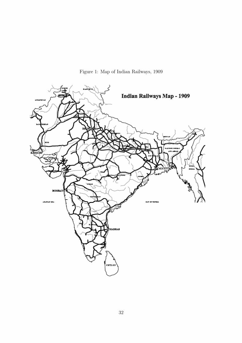
Figure 1: Map of Indian Railways, 1909

32

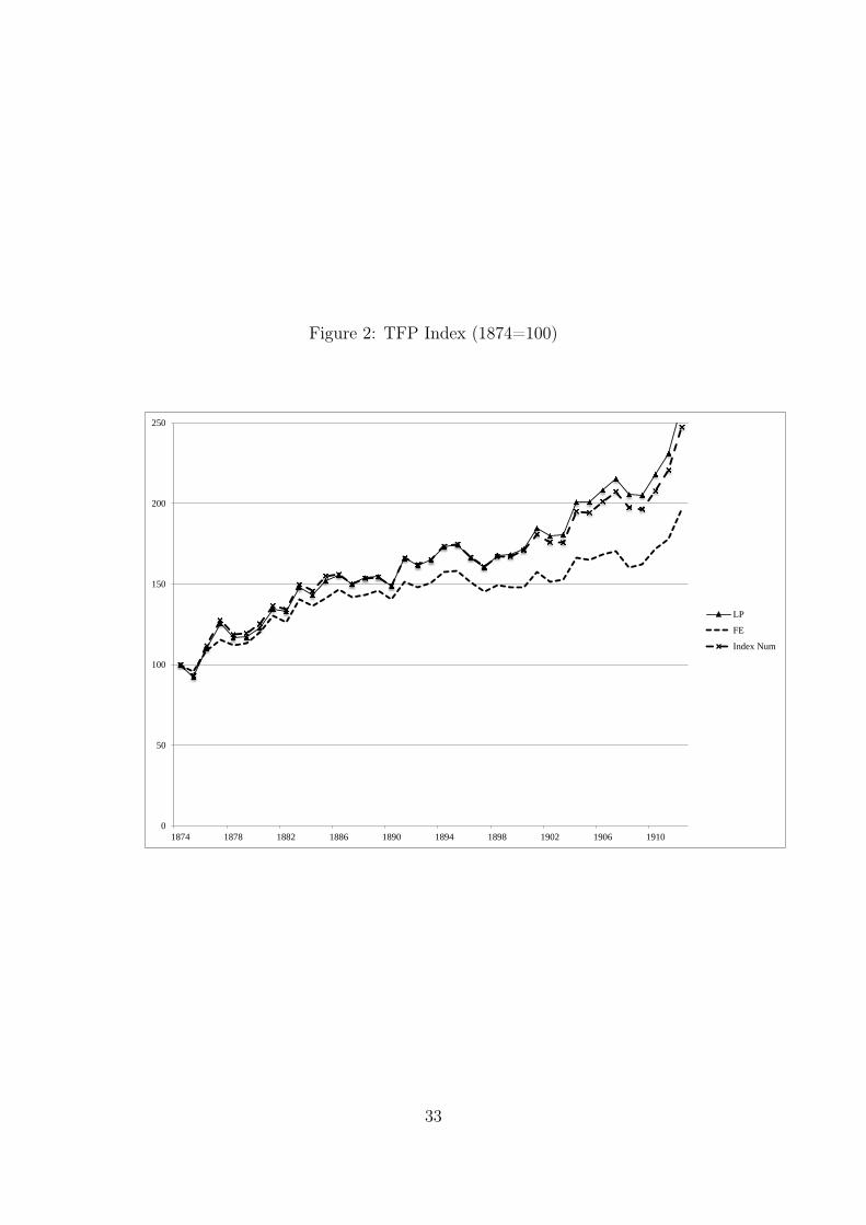
Figure 2: TFP Index (1874=100)

0

50

100

150

200

250

1874 1878 1882 1886 1890 1894 1898 1902 1906 1910

LP

FE

Index Num

33

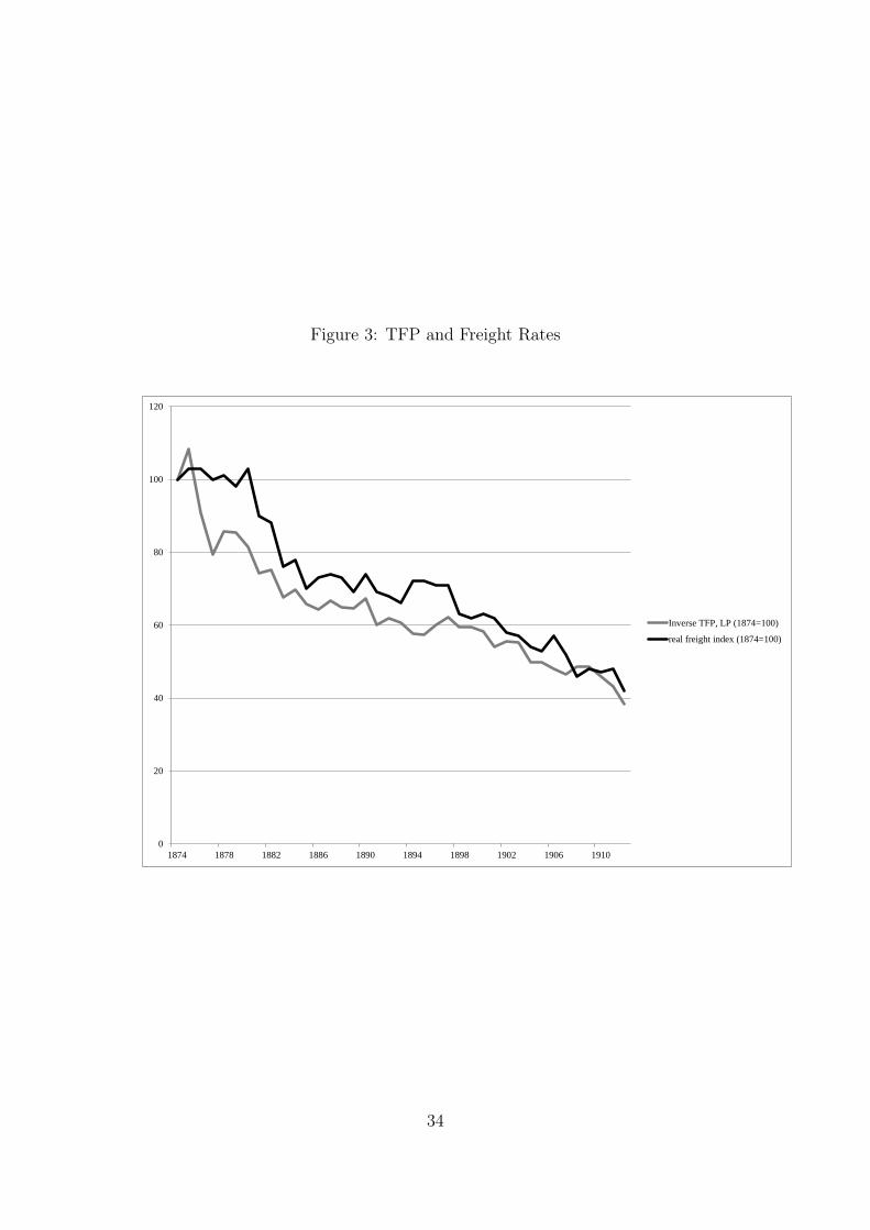
Figure 3: TFP and Freight Rates

0

20

40

60

80

100

120

1874 1878 1882 1886 1890 1894 1898 1902 1906 1910

Inverse TFP, LP (1874=100)

real freight index (1874=100)

34

Figure 4: Role of Reallocation in TFP Growth

-0.1

-0.05

0

0.05

0.1

0.15

0.2

1874 1878 1882 1886 1890 1894 1898 1902 1906 1910

TFP growth

reallocation

35

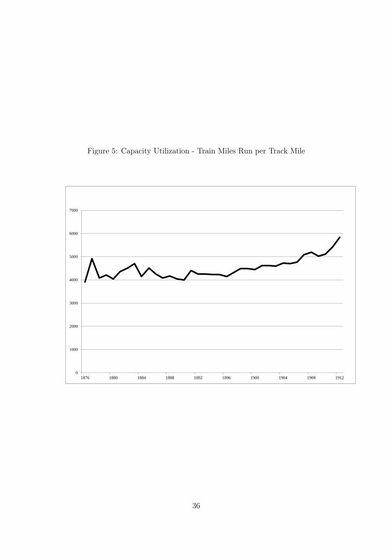
Figure 5: Capacity Utilization - Train Miles Run per Track Mile

0

1000

2000

3000

4000

5000

6000

7000

1876 1880 1884 1888 1892 1896 1900 1904 1908 1912

36

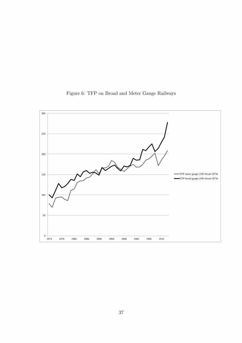
Figure 6: TFP on Broad and Meter Gauge Railways

0

50

100

150

200

250

300

1874 1878 1882 1886 1890 1894 1898 1902 1906 1910

TFP meter gauge (100=broad 1874)

TFP broad gauge (100=broad 1874)

37

Railway name Gauge Entry ExitGreat Indian Peninsula Broad pre-74 n.a.East Indian Broad pre-74 n.a.Madras Broad pre-74 n.a.Bombay, Baroda and Central India Broad pre-74 n.a.Northwestern (Sind, Punjab and Delhi pre-1885) Broad pre-74 n.a.South Indian Meter pre-74 n.a.Eastern Bengal Mixed pre-74 n.a.Oudh and Rohilkhand Broad pre-74 n.a.Rajputana Malwa Meter pre-74 n.a.Nizam Mixed 1878 n.a.Bengal and Northwestern Meter 1884 n.a.Burma Meter 1878 n.a.Bengal Nagpur Broad 1880 n.a.Southern Mahratta Meter 1882 1908Assam Bengal Meter 1896 n.a.Bhavnagar-Gondal-Junagad-Porbandar Meter 1882 n.a.East Coast Broad 1894 1901Udaipur Chittoor Meter 1900 n.a.Rohilkhand and Kumaon Meter 1885 n.a.Jodhpore-Bikaneer Meter 1886 n.a.Dhond-Manmad Meter 1879 1881Wardha Coal Broad 1879 1891Indian Midland Broad 1888 1901Punjab Northern Broad 1875 1886Indus Valley Broad 1879 1886Calcutta and Southeastern Broad pre-1874 1884Dacca Meter 1885 1887Bengal Central Broad 1897 1905Muttra Hathras Meter 1879 1886Holkar and Sindia-Neemuch Meter 1875 1881Tirhoot Meter 1876 1889Northern Bengal Meter 1878 1887Sources: See text for details.

Table 1: Railways in Sample

Variable Obs Mean Std. Dev Min Max

Ton miles (millions) 732 296 532 0 5,467Passenger miles (millions) 732 330 388 2 2,214Output (cost weights) 732 319 478 2 4,463

Labor 732 15,867 18,104 135 96,542Fuel (Kurharbaree coal, thousands) 732 80 116 0 755Miles 732 959 828 28 4,737Engines 732 210 234 2 1,151Vehicles 732 4,717 4,751 61 26,845Capital (in millions of 1912 rupees) 732 147 172 1 1,029

1874-1912 1874-79 1880-89 1890-99 1900-12

Output/Labor 2.04% 1.4% 2.0% 1.0% 3.1%Output/Fuel 0.91% 3.0% 2.1% -1.2% 0.9%Output/Capital (in rupees) 3.02% 4.6% 2.2% 2.0% 3.8%Output/Miles 2.44% 3.7% 0.1% 1.3% 4.7%Output/Engines 2.51% 2.6% 1.0% 2.4% 3.7%Output/Vehicles 1.70% 0.9% 0.5% 1.9% 2.8%

Source: Administration Reports on Railways in India, 1874 to 1912.

Table 2: Summary Statistics

Annual Growth Rate (in %)

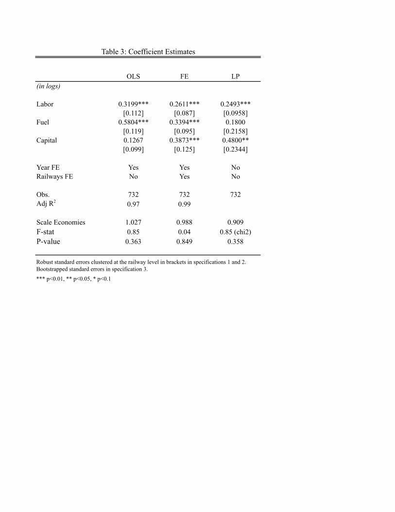
OLS FE LP(in logs)

Labor 0.3199*** 0.2611*** 0.2493***[0.112] [0.087] [0.0958]

Fuel 0.5804*** 0.3394*** 0.1800[0.119] [0.095] [0.2158]

Capital 0.1267 0.3873*** 0.4800**[0.099] [0.125] [0.2344]

Year FE Yes Yes NoRailways FE No Yes No

Obs. 732 732 732Adj R2 0.97 0.99

Scale Economies 1.027 0.988 0.909F-stat 0.85 0.04 0.85 (chi2)P-value 0.363 0.849 0.358

*** p<0.01, ** p<0.05, * p<0.1

Table 3: Coefficient Estimates

Robust standard errors clustered at the railway level in brackets in specifications 1 and 2. Bootstrapped standard errors in specification 3.

OLS FE LP IN (Indian W.)

OLS 1FE 0.81 1LP 0.61 0.94 1IN (Indian W.) 0.68 0.98 0.94 1

1874-1912 1874-79 1880-89 1890-99 1900-12

OLS 1.24 1.85 2.42 -0.39 1.39FE 1.99 2.89 2.59 0.34 2.47Levinsohn and Petrin 2.55 3.21 2.81 0.85 3.42Index Number 2.41 3.64 2.59 0.80 3.06

Table 4: Correlation Coefficients Across TFP Models

Table 5: Estimates of TFP Growth RatesAnnual Growth Rate (in %)

Country Years Estimation Method TFP Growth

India 1874-1912 Production Function (LP) 2.55India 1874-1912 Index Number 2.41US 1870-1910 Index Number 2.10Britain 1874-1912 Index Number 0.80Spain 1870-1913 Cost Function 1.50

Table 6: Railway TFP Growth Across Countries

Sources: For the US see Fishlow (1966), for Britain see Crafts, Mills, and Mulatu (2009), for Canada see Green (1986), for Spain see Herranz-Loncán (2006).

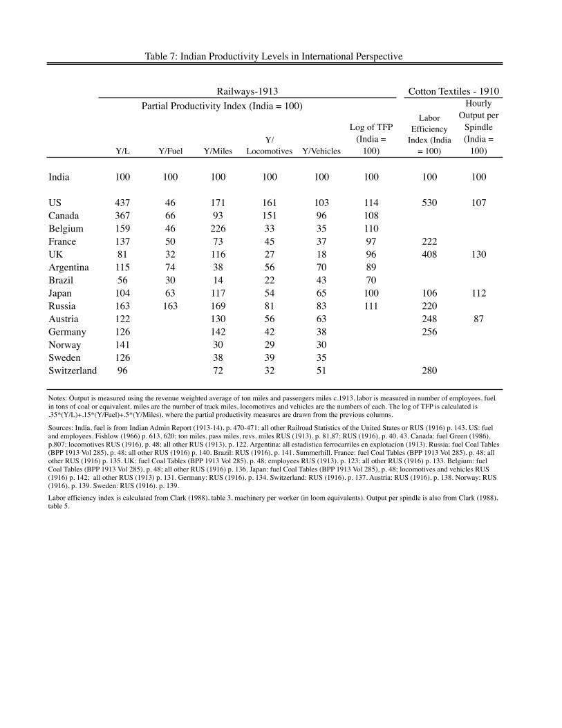
Y/L Y/Fuel Y/MilesY/

Locomotives Y/Vehicles

India 100 100 100 100 100 100 100 100

US 437 46 171 161 103 114 530 107Canada 367 66 93 151 96 108Belgium 159 46 226 33 35 110France 137 50 73 45 37 97 222UK 81 32 116 27 18 96 408 130Argentina 115 74 38 56 70 89Brazil 56 30 14 22 43 70Japan 104 63 117 54 65 100 106 112Russia 163 163 169 81 83 111 220Austria 122 130 56 63 248 87Germany 126 142 42 38 256Norway 141 30 29 30Sweden 126 38 39 35Switzerland 96 72 32 51 280

Labor efficiency index is calculated from Clark (1988), table 3, machinery per worker (in loom equivalents). Output per spindle is also from Clark (1988), table 5.

Partial Productivity Index (India = 100)

Log of TFP (India =

100)

Railways-1913

Labor Efficiency

Index (India = 100)

Table 7: Indian Productivity Levels in International Perspective

Hourly Output per

Spindle (India =

100)

Cotton Textiles - 1910

Notes: Output is measured using the revenue weighted average of ton miles and passengers miles c.1913, labor is measured in number of employees, fuel in tons of coal or equivalent, miles are the number of track miles, locomotives and vehicles are the numbers of each. The log of TFP is calculated is .35*(Y/L)+.15*(Y/Fuel)+.5*(Y/Miles), where the partial productivity measures are drawn from the previous columns.

Sources: India, fuel is from Indian Admin Report (1913-14), p. 470-471; all other Railroad Statistics of the United States or RUS (1916) p. 143. US: fuel and employees, Fishlow (1966) p. 613, 620; ton miles, pass miles, revs, miles RUS (1913), p. 81,87; RUS (1916), p. 40, 43. Canada: fuel Green (1986), p.807; locomotives RUS (1916), p. 48; all other RUS (1913), p. 122. Argentina: all estadistica ferrocarriles en explotacion (1913). Russia: fuel Coal Tables (BPP 1913 Vol 285), p. 48; all other RUS (1916) p. 140. Brazil: RUS (1916), p. 141. Summerhill. France: fuel Coal Tables (BPP 1913 Vol 285), p. 48; all other RUS (1916) p. 135. UK: fuel Coal Tables (BPP 1913 Vol 285), p. 48; employees RUS (1913), p. 123; all other RUS (1916) p. 133. Belgium: fuel Coal Tables (BPP 1913 Vol 285), p. 48; all other RUS (1916) p. 136. Japan: fuel Coal Tables (BPP 1913 Vol 285), p. 48; locomotives and vehicles RUS (1916) p. 142; all other RUS (1913) p. 131. Germany: RUS (1916), p. 134. Switzerland: RUS (1916), p. 137. Austria: RUS (1916), p. 138. Norway: RUS (1916), p. 139. Sweden: RUS (1916), p. 139.

India India 1874-1912 1874-1912

Railway Capital Stock Growth / Worker 1.46 1.46Railway Profits Share in National Income 0.015 0.015Railway Capital Contribution 0.02 0.02

Railway TFP Growth 1.99 2.55Railway Share in National Output 0.03 0.03Railway TFP Contribution 0.06 0.08

Total Railway Contribution w/o Spillovers 0.08 0.1(as % of GDP per capita growth) 13.33 16.67

TFP Estimation method FE LPSource: See text for details on sources.

Table 8: Contribution of Indian Railways to Annual GDP per capita Growth

OLS FE(in logs)

Train Miles Run/ 0.2709** 0.5245***Track Mile [0.117] [0.071]

Obs 710 710

Year FE Yes YesRailways FE No Yes

TFP Growth Rate Net of Utilization1.14 1.73

1.24 1.99

Table 9: Capacity Utilization or TFP?

TFP Growth Rate (Table 5)

Robust standard errors clustered at the railway level in brackets. *** p<0.01, ** p<0.05, * p<0.1. Regressions include capital (in rupees), labor and fuel as in Table 3.

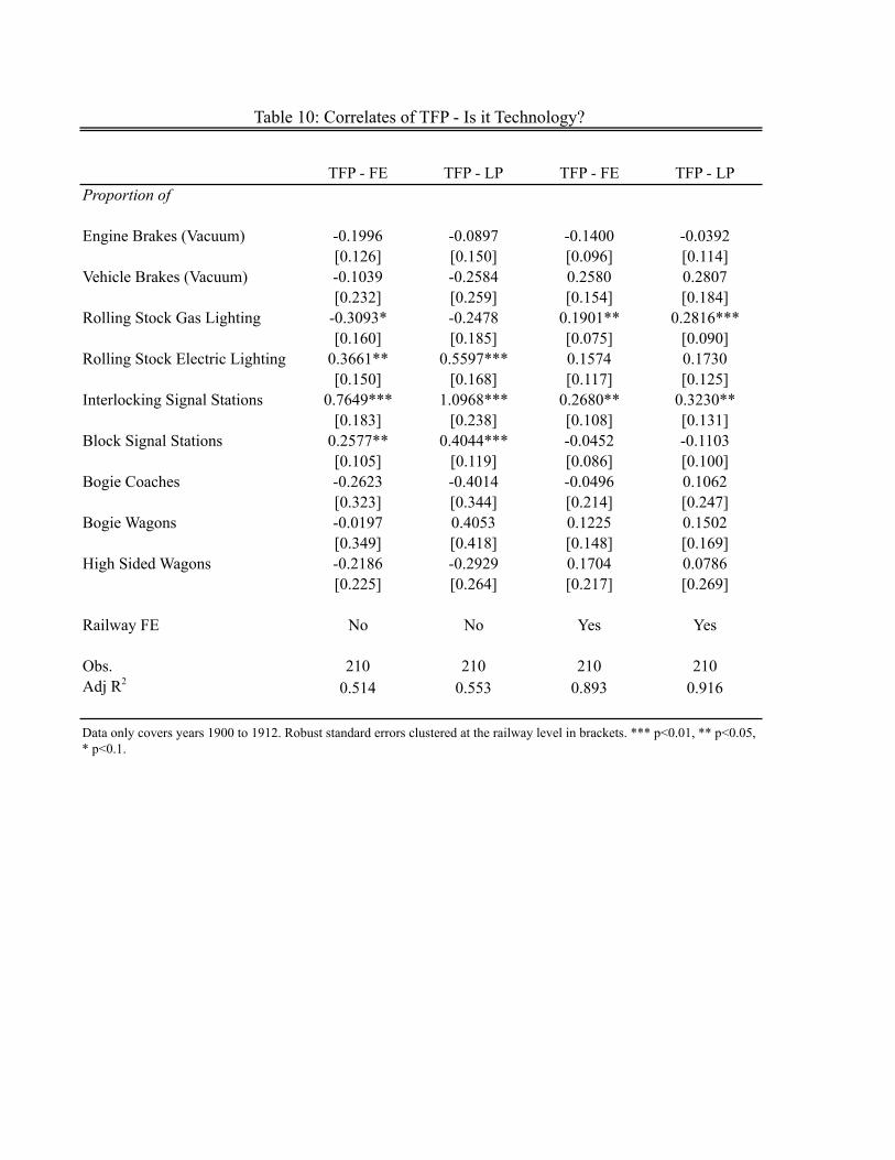
TFP - FE TFP - LP TFP - FE TFP - LPProportion of

Engine Brakes (Vacuum) -0.1996 -0.0897 -0.1400 -0.0392[0.126] [0.150] [0.096] [0.114]

Vehicle Brakes (Vacuum) -0.1039 -0.2584 0.2580 0.2807[0.232] [0.259] [0.154] [0.184]

Rolling Stock Gas Lighting -0.3093* -0.2478 0.1901** 0.2816***[0.160] [0.185] [0.075] [0.090]

Rolling Stock Electric Lighting 0.3661** 0.5597*** 0.1574 0.1730[0.150] [0.168] [0.117] [0.125]

Interlocking Signal Stations 0.7649*** 1.0968*** 0.2680** 0.3230**[0.183] [0.238] [0.108] [0.131]

Block Signal Stations 0.2577** 0.4044*** -0.0452 -0.1103[0.105] [0.119] [0.086] [0.100]

Bogie Coaches -0.2623 -0.4014 -0.0496 0.1062[0.323] [0.344] [0.214] [0.247]

Bogie Wagons -0.0197 0.4053 0.1225 0.1502[0.349] [0.418] [0.148] [0.169]

High Sided Wagons -0.2186 -0.2929 0.1704 0.0786[0.225] [0.264] [0.217] [0.269]

Railway FE No No Yes Yes

Obs. 210 210 210 210Adj R2 0.514 0.553 0.893 0.916

Data only covers years 1900 to 1912. Robust standard errors clustered at the railway level in brackets. *** p<0.01, ** p<0.05, * p<0.1.

Table 10: Correlates of TFP - Is it Technology?