engineering risk benefit analysis - mit opencourseware · p e h p h p e h p h p h e. rpra 5. data...

RPRA 5. Data Analysis 1

Engineering Risk Benefit Analysis1.155, 2.943, 3.577, 6.938, 10.816, 13.621, 16.862, 22.82,

ESD.72, ESD.721

RPRA 5. Data Analysis

George E. ApostolakisMassachusetts Institute of Technology

Spring 2007


Statistical Inference

Theoretical Model Evidence

Failure distribution, Sample, e.g.,e.g., {t1,…,tn}

• How do we estimate from the evidence?• How confident are we in this estimate?• Two methods:

– Classical (frequentist) statistics– Bayesian statistics

te)t(f λ−λ=

λ


Random Samples

• The observed values are independent and the underlying distribution is constant.

• Sample mean:

• Sample variance:

∑=n

1it

n1t

∑ −−

=n

1

2i

2 )tt()1n(

1s


The Method of Moments: Exponential Distribution

• Set the theoretical moments equal to the sample moments and determine the values of the parameters of the theoretical distribution.

• Exponential distribution:

Sample: {10.2, 54.0, 23.3, 41.2, 73.2, 28.0} hrs

t1 =λ

32.386

9.229)282.732.413.23542.10(61t ==+++++=

1hr026.032.38

1 −==λ;hrs32.38MTTF =


The Method of Moments:Normal Distribution

• Sample: {5.5, 4.7, 6.7, 5.6, 5.7}

μ===++++= 68.55

4.285

)7.56.57.67.47.5(x

032.2)68.57.5(...)68.55.5()xx(5

1

222i =−++−=−∑

σ==

=−

=

713.0s

508.0)15(

032.2s2


The Method of Moments:Poisson Distribution

• Sample: {r events in t}

• Average number of events: r

• {3 eqs in 7 years}

trrt =λ⇒=λ

1yr43.073 −==λ⇒


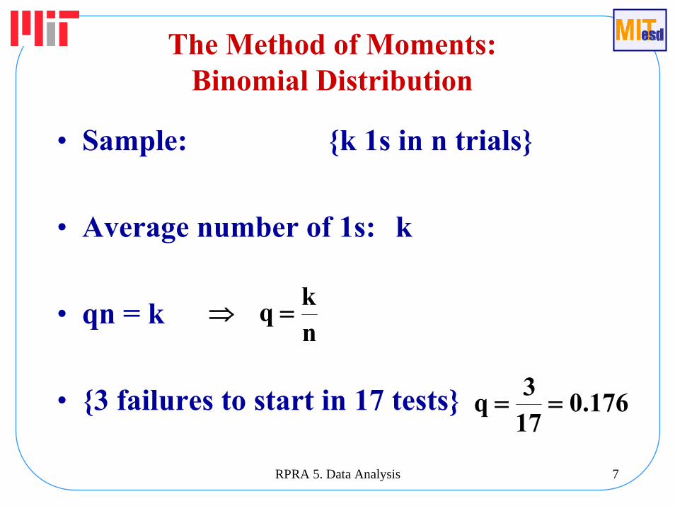
The Method of Moments:Binomial Distribution

• Sample: {k 1s in n trials}

• Average number of 1s: k

• qn = k

• {3 failures to start in 17 tests}

nkq =⇒

176.0173q ==


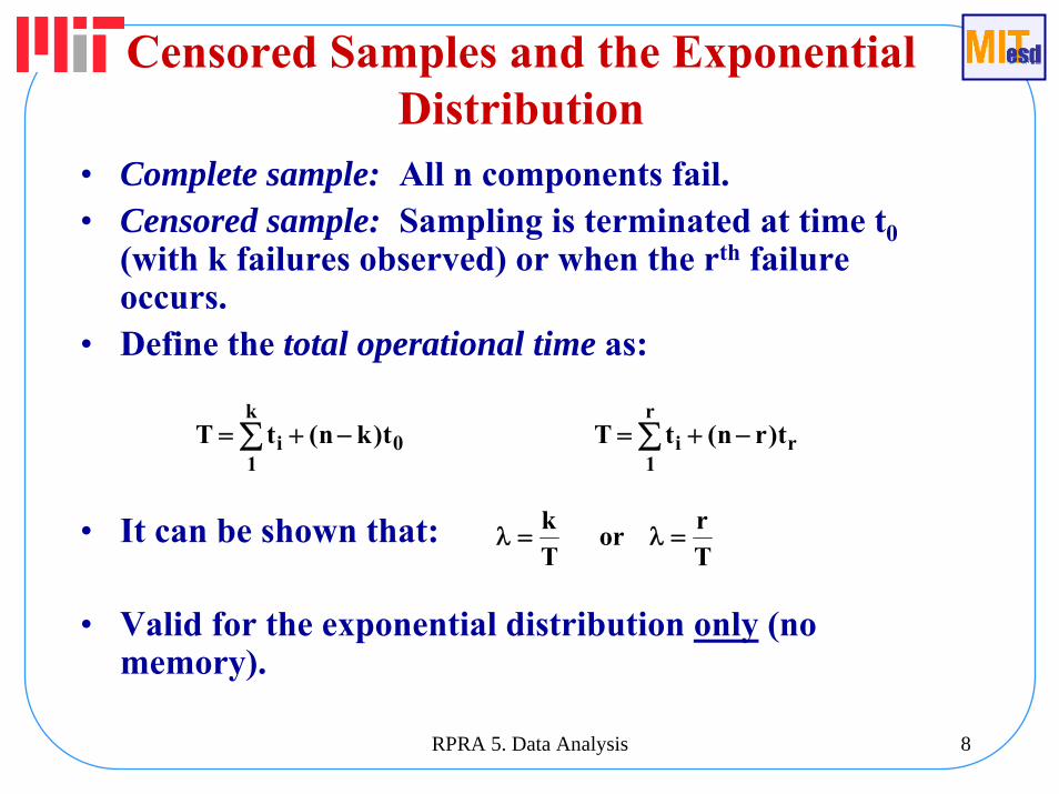
Censored Samples and the Exponential Distribution

• Complete sample: All n components fail.• Censored sample: Sampling is terminated at time t0

(with k failures observed) or when the rth failure occurs.

• Define the total operational time as:

• It can be shown that:

• Valid for the exponential distribution only (no memory).

∑ −+=k

10i t)kn(tT ∑ −+=

r

1ri t)rn(tT

Tror

Tk =λ=λ


Example

• Sample: 15 components are tested and the test is terminated when the 6th failure occurs.

• The observed failure times are:{10.2, 23.3, 28.0, 41.2, 54.0, 73.2} hrs

• The total operational time is:

• Therefore

7.8882.73)615(2.73542.41283.232.10T =−++++++=

13 hr10x75.67.888

6 −−==λ


Bayesian Methods• Recall Bayes’ Theorem (slide 16, RPRA 2):

• Prior information can be utilized via the prior distribution.

• Evidence other than statistical can be accommodated via the likelihood function.

PosteriorProbability

PriorProbability

Likelihood of theEvidence

( ) ( ) ( )( ) ( )∑

= N

1ii

iii

HPHEP

HPHEPEHP


The Model of the World

– Deterministic, e.g., a mechanistic computer code

– Probabilistic (Aleatory), e.g., R(t/ ) = exp(- t)

– The MOW deals with observable quantities.

– Both deterministic and aleatory models of the world have assumptions and parameters.

– How confident are we about the validity of these assumptions and the numerical values of the parameters?

λ λ


The Epistemic Model

• Uncertainties in assumptions are not handled routinely. If necessary, sensitivity studies are performed.

• The epistemic model deals with non-observablequantities.

• Parameter uncertainties are reflected on appropriate probability distributions.

• For the failure rate: π( ) d = Pr(the failure rate has a value in d about )λ

λλ

λ


Unconditional (predictive) probability

∫ λλπλ= d)()/t(R)t(R


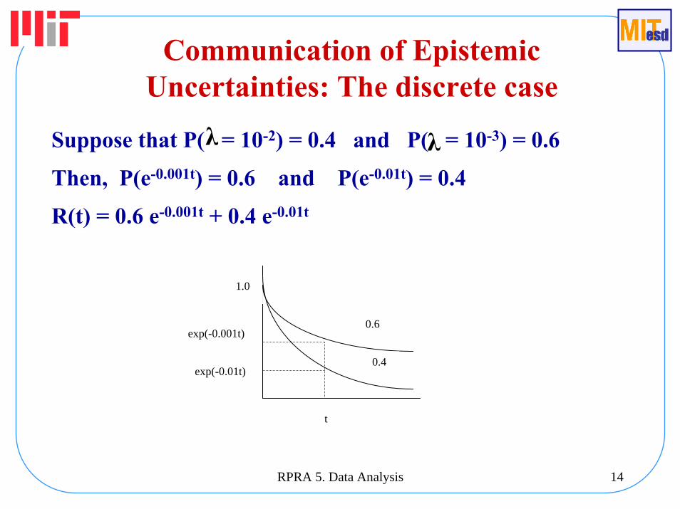
Communication of Epistemic Uncertainties: The discrete case

Suppose that P( = 10-2) = 0.4 and P( = 10-3) = 0.6

Then, P(e-0.001t) = 0.6 and P(e-0.01t) = 0.4

R(t) = 0.6 e-0.001t + 0.4 e-0.01t

t

1.0

exp(-0.001t)

exp(-0.01t)

0.6

0.4

λλ


Communication of Epistemic Uncertainties: The continuous case


Risk Curves

Figure by MIT OCW.

1,000100Public Acute Fatalities

Prob

abili

ty o

f Exc

eede

nce

1011.0E-09

1.0E-08

1.0E-07

1.0E-06

1.0E-05

1.0E-0495th Percentile

Mean

Median

5th Percentile


The Quantification of Judgment

• Where does the epistemic distribution π( ) come from?

• Both substantive and normative “goodness” are required.

• Direct assessments of parameters like failure rates should be avoided.

• A reasonable measure of central tendency to estimate is the median.

• Upper and lower percentiles can also be estimated.

λ


The lognormal distribution

• It is very common to use the lognormal distribution as the epistemic distribution of failure rates.

⎥⎦

⎤⎢⎣

⎡σμ−λ

−σλπ

=λπ 2

2

2)(lnexp

21)(

UB = = exp( + 1.645 )

LB = = exp( - 1.645 )

95λ

05λ μ

μ

σ

σ


Pumps

Component/PrimaryFailure Modes

Assessed ValuesLower Bound Upper Bound

Valves

Failure to start, Qd:

Failure to operate, Qd:



Failure to open, Qd:

Failure to open, Qd:

Plug, Qd:

Plug, Qd:

Plug, Qd:

Failure to run, λo:

< 3" diameter, λo:> 3" diameter, λo:

(Normal Environments)

3 x 10-4/d 3 x 10-3/d3 x 10-6/hr 3 x 10-4/hr

3 x 10-4/d 3 x 10-3/d

3 x 10-5/d 3 x 10-4/d

3 x 10-4/d 3 x 10-3/dPlug, Qd: 3 x 10-5/d 3 x 10-4/d

1 x 10-4/d 1 x 10-3/d

3 x 10-5/d 3 x 10-4/d

3 x 10-5/d 3 x 10-4/d

3 x 10-6/d 3 x 10-5/d

3 x 10-5/d 3 x 10-4/d

3 x 10-11/hr 3 x 10-8/hr3 x 10-12/hr 3 x 10-9/hr

1 x 10-4/d 1 x 10-3/d

Motor Operated

Solenoid Operated

Check

Relief

Manual

Plug/rupture

MechanicalFailure to engage/disengage

Pipe

Clutches

Mechanical Hardware

Air Operated

Table by MIT OCW.

Adapted from Rasmussen, et al."The Reactor Safety Study."WASH-1400, US Nuclear RegulatoryCommission, 1975.


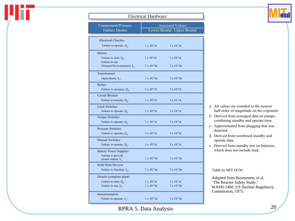
Table by MIT OCW.

Adapted from Rasmussen, et al.The Reactor Safety Study."

WASH-1400, US Nuclear RegulatoryCommission, 1975.

"

Motors

Failure to start, Q 1 x 10-3d: 1 x 10-4/d /d

Failure to run(Normal Environments), λ -5

o: 3 x 10-6/hr 3 x 10 /hr

Transformers

Open/shorts, λ 3 x 10-7/hr 3 x 10-6o: /hr

Relays

Failure to energize, Q -5 -4d: 3 x 10 /d 3 x 10 /d

Circuit Breaker

Failure to transfer, Qd: 3 x 10-4/d 3 x 10-3/d

Limit SwitchesFailure to operate, Q 1 x 10-3

d: 1 x 10-4/d /d

Torque Switches

Failure to operate, Q : 3 x 10-5/d -4d

3 x 10 /d

Pressure Switches

Failure to operate, Qd: 3 x 10-5/d 3 x 10-4/d

Manual Switches

Failure to operate, Q : 3 x 10-6 -5d

/d 3 x 10 /d

Battery Power SuppliesFailure to provideproper output, λ : 1 x 10-6/hr 1 x 10-5/hr

s

Solid State Devices

Failure to function, λo: 3 x 10-7/hr 3 x 10-5/hr

Diesels (complete plant)

Failure to start, Q -2d: 1 x 10 /d 1 x 10-1/d

Failure to run, λo: 3 x 10-4/hr 3 x 10-2/hr

Instrumentation

Failure to operate, λo: 1 x 10-7/hr 1 x 10-5/hr

Electrical Hardware

Electrical Clutches

Failure to operate, Qd: 1 x 10-4/d 1 x 10-3/d

Component/Primary Assessed ValuesFailure Modes Lower Bound Upper Bound

a. All values are rounded to the nearest half order of magnitude on the exponent.

b. Derived from averaged data on pumps, combining standby and operate time.

c. Approximated from plugging that was detected.

d. Derived from combined standby and operate data.

e. Derived from standby test on batteries, which does not include load.


Example

1350 hr10x3)μexp(λ −−==

1295 hr10x3)σ645.1μexp(λ −−=+=

40.1σ,81.5μThen =−=

132

hr10x8)2σμexp(]λ[E −−=+=

1405 hr10x3)σ645.1μexp(λ −−=−=

Lognormal prior distribution with median and 95th percentile given as:


Updating Epistemic Distributions

• Bayes’ Theorem allows us to incorporate new evidence into the epistemic distribution.

∫=

λd)λ(π)λ/E(L)λ(π)λ/E(L)E/λ('π


Example of Bayesian updating of epistemic distributions

• Five components were tested for 100 hours each and no failures were observed.

• Since the reliability of each component is exp(-100 ), the likelihood function is:

• L(E/ ) = P(comp. 1 did not fail AND comp. 2 did not fail AND… comp. 5 did not fail) = exp(-100 ) x exp(-100 ) x…x exp(-100 ) = exp(-500 )

• L(E/ ) = exp(-500 )– Note: The classical statistics point estimate is zero since no

failures were observed.

λλ

λ

λ

λλ

λ

λ


Prior ( ) and posterior ( ) distributions

λ

1e-4 1e-3 1e-2 1e-1

Pro

babi

lity

0.000

0.001

0.002

0.003

0.004

0.005

0.006

0.007

0.008


Impact of the evidence

Mean(hr-1)

95th

(hr-1)Median

(hr-1)5th

(hr-1)Prior distr.

8.0x10-3 3.0x10-2 3x10-3 3.0x10-3

Posterior distr.

1.3x10-3 3.7x10-3 9x10-4 1.5x10-4


Selected References

• Proceedings of Workshop on Model Uncertainty: Its Characterization and Quantification, A. Mosleh, N. Siu, C. Smidts, and C. Lui, Eds., Center for Reliability Engineering, University of Maryland, College Park, MD, 1995.

• Reliability Engineering and System Safety, Special Issue on the Treatment of Aleatory and Epistemic Uncertainty, J.C. Helton and D.E. Burmaster, Guest Editors., vol. 54, Nos. 2-3, Elsevier Science, 1996.

• Apostolakis, G., “The Distinction between Aleatory and Epistemic Uncertainties is Important: An Example from the Inclusion of Aging Effects into PSA,” Proceedings of PSA ‘99, International Topical Meeting on Probabilistic Safety Assessment, pp. 135-142, Washington, DC, August 22 - 26, 1999, American Nuclear Society, La Grange Park, Illinois.

engineering risk benefit analysis - mit opencourseware · p e h p h p e h p h p h e. rpra 5. data...

Documents