Constant-pressure nested sampling with atomistic dynamics

Robert J.N. Baldock,1, ∗ Noam Bernstein,2 K. Michael Salerno,3 Lıvia B. Partay,4 and Gabor Csanyi5

1Theory and Simulation of Materials (THEOS), and National Centre forComputational Design and Discovery of Novel Materials (MARVEL),

Ecole Polytechnique Federale de Lausanne, CH-1015 Lausanne, Switzerland2Center for Materials Physics and Technology, Naval Research Laboratory, Washington, DC 20375, USA

3National Research Council Associateship Program,resident at the U.S. Naval Research Laboratory, Washington DC 20375, USA

4Department of Chemistry, University of Reading, United Kingdom5Engineering Laboratory, University of Cambridge, United Kingdom

The nested sampling algorithm has been shown to be a general method for calculating the pressure-temperature-composition phase diagrams of materials. While the previous implementation usedsingle-particle Monte Carlo moves, these are inefficient for condensed systems with general interac-tions where single-particle moves cannot be evaluated faster than the energy of the whole system.Here we enhance the method by using all-particle moves: either Galilean Monte Carlo or a totalenthalpy Hamiltonian Monte Carlo algorithm, introduced in this paper. We show that these algo-rithms enable the determination of phase transition temperatures with equivalent accuracy to theprevious method at 1/N of the cost for an N -particle system with general interactions, or at equalcost when single particle moves can be done in 1/N of the cost of a full N -particle energy evaluation.We demonstrate this speedup for the freezing and condensation transitions of the Lennard-Jonessystem and show the utility of the algorithms by calculating the order-disorder phase transition ofa binary Lennard-Jones model alloy, the eutectic of copper-gold, the density anomaly of water andthe condensation and solidification of bead-spring polymers. The nested sampling method with allthree algorithms is implemented in the pymatnest software.

I. INTRODUCTION

The ability to predict the behavior of materials un-der a variety of conditions is important in both academicand industrial settings. In principle, statistical mechan-ics enables the prediction of the properties of materi-als in thermodynamic equilibrium from the microscopicinteraction of atoms. Computer simulation is the toolfor using numerical statistical mechanics in practice, anda wide variety of models and approximations are usedfor atomic interactions, all the way from the electronicSchrodinger equation to simple hard spheres. The equi-librium pressure-temperature phase diagram for a givencomposition is one of the most fundamental propertiesof a material, and forms the basis for making, changing,designing, or in general, just thinking about the material.

The common approach is to use different computa-tional methods for resolving each of the transitions be-tween the phases, or for comparing the stability of par-ticular combinations of phases. This requires the priorknowledge of a list of proposed phases or crystal struc-tures at each set of thermodynamic parameters. In aprevious paper [1] we introduced a nested sampling (NS)algorithm [2, 3] that enables the automated calculationof complete pressure-temperature-composition phase di-agrams. The nested sampling algorithm constitutes asingle method for resolving all phase transitions auto-matically in the sense that no prior knowledge of thephases is required.

∗ rjnbaldock@gmail.com

The algorithm in [1] used Gibbs sampling, i.e. singleparticle Monte Carlo (SP-MC) moves, to explore con-figuration space. For some interactions, which we termseparable, the energy change of an N -particle system dueto the displacement of a single particle can be calculatedin 1/N times the cost of evaluating the energy of thewhole system. Thus, for separable interactions, the costof an N -particle sweep is equal to the cost of a single full-system energy/force evaluation. For these cases Gibbssampling is efficient. However, interactions in generalare not separable, and if a single-particle move is just ascostly as a full-system evaluation, a sweep that moves ev-ery particle costs N times more than a single full-systemenergy/force calculation. All-particle MC moves can beused in principle, but it is well known that making suchmoves in random directions leads to very slow explorationin condensed phases (liquids, solids), because maintain-ing a finite MC acceptance rate requires that the dis-placement of each atom become smaller as the systemsize increases [4].

Here we replace Gibbs sampling by either one of two al-gorithms that use efficient all-particle moves inspired bythe Hamiltonian Monte Carlo (HMC) method [5]. Thepurpose of this paper is to show how these algorithmscan be utilized efficiently in the case of nested sampling.One is a total enthalpy HMC (TE-HMC) introduced inthis paper, which takes advantage of standard moleculardynamics (MD) implemented in many simulation pack-ages. The other is Galilean Monte Carlo (GMC) [6, 7],which is not as widely available, but does not suffer fromthe breakdown of ergodicity that the TE-HMC algorithmmay experience for systems with a large number of par-

arX

iv:1

710.

1108

5v2

[co

nd-m

at.s

tat-

mec

h] 1

6 N

ov 2

017

2

ticles. We compare the efficiency of these two methodswith that of Gibbs sampling, and find that they requirecomparable numbers of whole-system energy/force eval-uations, leading to a factor of 1/N reduction in compu-tational time for general inter-particle interactions.

The GMC and TE-HMC algorithms use inter-particleforce information to move all particles coherently along“soft” degrees of freedom, and therefore explore fasterthan simple diffusion, at least over short-time scales. Ef-fectively, short trajectories are all-particle MC move pro-posals with large step lengths that still lead to reasonableMC acceptance probabilities. Over the time scale of anentire Markov chain Monte Carlo (MCMC) walk, the mo-tion is still diffusive, but the short time coherence helpsGMC and TE-HMC explore configuration space muchfaster than randomly oriented all-particle moves. UsingGMC or TE-HMC enables the simulation of a wide rangeof phase transitions in atomistic and particle systemswith NS, including chemical ordering in binary Lennard-Jones (LJ), the eutectic of copper-gold alloys, freezingof water, and the transitions of a coarse-grained bead-spring polymer model. Parallel implementations of bothalgorithms are available in the pymatnest python soft-ware package [8], using the LAMMPS package [9] for thedynamics.

II. THE NESTED SAMPLING METHOD

The nested sampling algorithm with constant pres-sure and flexible boundary conditions (i.e. with variableperiodic cell shape and volume) calculates the cumula-

tive density of states, χ(H), at fixed pressure P , where

H = U + PV is the configurational enthalpy, U(r) isthe potential energy function, and V is the volume ofthe system. From the cumulative density of states, onecan calculate the partition function and heat capacity asexplicit functions of temperature. Nested sampling alsoreturns a series of atomic configurations, from which onemay compute ensemble averages of observables and freeenergy landscapes [1].

The key idea of nested sampling is that it constructs a

series of decreasing enthalpy levels {Hsupi }, each of which

bounds from above a volume of configuration space χi,with the property that χi is approximately a constantfactor smaller than the volume χi−1 of the level above.The constant pressure partition function, and its approx-imation in nested sampling, are then given by

∆ (N,P, β) =βP

N !

(2πm

βh2

)3N/2 ∫ ∞

−∞dH

∂χ

∂He−βH (1)

≈ βP

N !

(2πm

βh2

)3N/2∑

i

(χi−1 − χi) e−βHsupi .

(2)

Here N is the number of particles of mass m, h is Planck’s

constant and ∂χ/∂H is the density of enthalpy states.

To calculate the absolute value of the partition func-tion (2), we must possess the absolute values of the con-figuration space volumes {χi}. The volumes {χi} arespecified in NS as a decreasing geometric progression,starting from χ0, which is the total (finite) volume of theconfiguration space. The configuration space must there-fore be compact. In order to ensure that we are samplingfrom a compact configuration space, the simulation cellvolume V is restricted to be less than a maximum valueV0, chosen to be sufficiently large as to correspond to analmost ideal gas. The total configuration space volume istherefore χ0 = V N+1

0 /(N + 1). Restricting the samplingto V < V0 allows a good approximation of the partitionfunction provided kBT � PV0 [1].

The simulation cell is periodic, and is represented by h,a 3×3 matrix of lattice vectors that relates the Cartesianpositions of the particles r to the fractional coordinatess by r = hs. The volume of the simulation cell is V =deth, and h0 = hV −1/3 is the image of the unit cellnormalized to unit volume. The NS algorithm maintainsa pool of K configurations drawn from

Prob(s,h0, V |V0, H

sup, d0

)∝ V Nδ (deth0 − 1)

×Θ(Hsup − H

)Θ (V0 − V )

×3N∏

i=1

Θ(si)Θ(1− si) Θ

(d0 −min

j 6=k

[1

hj0 × hk0

]),

(3)

where Θ is the Heaviside step function, hi0 are columns

of h0, and Hsup is a maximum configurational enthalpy.Thus, fractional particle coordinates s are uniformly dis-

tributed on (0, 1)3N , H is restricted to be smaller than

Hsup, and V is restricted to be smaller than V0. The lastterm in Eq. (3) restricts the simulation cell from becom-ing too thin (controlled by the parameter d0), thus avoid-ing unphysical correlations between interacting periodicimages [1]. For simple fluids of 64 atoms, d0 should beset no smaller than 0.65, while simulations with largernumbers of atoms can tolerate smaller values of d0 [1](see Appendix E). The probability distribution (3) cor-responds to a uniform distribution over the Cartesianparticle coordinates r, subject to the constraints above.

The simulation is initialized by drawing K configura-

tions from distribution (3), with Hsup = ∞. After ini-tialization, the NS algorithm performs the following loop,starting with i = 1.

1. From the set ofK configurations, record theKr ≥ 1samples with the highest configurational enthalpy,

{H}i. Use the lowest enthalpy from that set,

min{H}i, as the new enthalpy limit: Hsup ←min{H}i. The volume of configuration space with

enthalpy equal to or less than Hsup is χi ≈ χ0[(K−Kr + 1)/(K + 1)]i.

2. Remove the Kr samples with enthalpies {H}i fromthe pool of samples and generate Kr new config-

3

urations from the distribution (3), using the up-

dated value of Hsup. This is achieved by first choos-ing Kr random configurations from the pool of re-maining samples, creating clones of those configura-tions, and evolving the cloned configurations usinga MCMC algorithm that converges to the distribu-tion (3).

3. Set i← i+1, and return to step 1 unless a stoppingcriterion is met (see Appendix A).

The required values of K and the MCMC walk-length,L, depend on the system being studied. This behavioris described in Refs. [1–3, 10]. In addition, increasingKr allows for greater parallelization of the NS algorithm;however, increasing Kr−1

K also leads to greater error inthe estimates of {χi}, so care should be taken not tomake Kr−1

K too large (see Appendix B).

Thermodynamic expectation values and free energylandscapes can be computed using the samples recordedduring step 1 of the NS algorithm [1]. Representativeconfigurations can be sampled at any temperature sim-ply by choosing configurations at random, according totheir thermalized probabilities

pi (β) =(χi−1 − χi) e−βHi

∑i (χi−1 − χi) e−βHi

. (4)

Examining a small number of configurations chosen inthis way is often sufficient to understand which phaseoccurs at each temperature. This method was used tochoose the atomic configurations shown in Sec. IV.

III. MARKOV CHAIN MONTE CARLOALGORITHMS

To decorrelate the cloned configurations in step 2 of theNS algorithm we use a MCMC algorithm that convergesto the distribution (3) by applying two kinds of steps:cell steps, including changes to volume and shape, andparticle steps, including continuous motion in space and(for multicomponent systems) coordinate swaps betweenparticles of different types.

The cell steps include volume steps thatensure Prob(V ) ∝ V N , and shearing andstretching steps that lead to Prob(h0) ∝δ (deth0 − 1) Θ

(d0 −mini6=j

[1

hi0×h

j0

]), as required

by the target distribution [1]. The following subsectionsintroduce the algorithms for moving the configuration inthe space of the atomic coordinates.

A. Galilean Monte Carlo

In GMC [6, 7] one defines an infinite square-well po-

tential function HGMC,

HGMC (s, V,h0) =

{0 : H < Hsup,

∞ : H ≥ Hsup,(5)

which is equal to the logarithm of the desired probability

distribution: uniform over the allowed region, H < Hsup,and zero elsewhere. Note that we have omitted the con-straints on V and h0 from (5) since we use GMC toexplore only the atomic coordinates. Having defined

HGMC, one samples the fractional atomic coordinatess uniformly by performing standard Hamiltonian Monte

Carlo sampling [5] on the function HGMC. We follow theGMC approach proposed by Betancourt [7], which uses afixed number of force evaluations and therefore helps theload balance when parallelizing the algorithm (see Ap-pendix B). Our implementation, expressed for practicalconvenience of implementation in Cartesian coordinatesr rather than fractional coordinates s, is as follows.

At the start of each atomic GMC trajectory, save theinitial atomic coordinates r0. Generate a velocity v cho-sen uniformly from the surface of a 3N -dimensional hy-persphere of radius 1. Repeat the following loop L times:

1. Propagate the atomic coordinates r in the direc-tion of v for one step of length dt. The atomiccoordinates are now r∗.

2. If H ≥ Hsup, attempt to redirect the trajectoryback into the allowed region by reflecting velocitiesfrom the current position, by v ← v − 2(v · n)n,

where n = −∇rH/|∇rH|. Following velocity re-flection, propagation continues from r∗.

Finally, if at the end of the trajectory H ≥ Hsup, rejectthe trajectory and return to the initial atomic coordi-nates r0. Note that the reflection in step 2 does not occur

at the exact boundary H = Hsup, and this is essentialto maintain detailed balance. The acceptance rate of theGMC step is controlled by adjusting dt. There are sim-ilarities between GMC and the “hit and run” algorithmfor sampling convex volumes [11], and it remains to beseen whether the clear advantages over Gibbs samplinghave common underlying reasons [12].

B. Total enthalpy Hamiltonian Monte Carlo

One disadvantage of GMC is that when the boundary

of the allowed region of configuration space H < Hsup

is complicated, attempts to reflect the sampler back intothe allowed region fail frequently, and reflection furtherinto the disallowed region often leads to rejection of theentire trajectory, thus overall driving down the optimal

4

step size. Hamiltonian (constant energy) molecular dy-namics, on the other hand, can generate nearly constanttotal energy trajectories using comparatively large stepsizes, and use the exchange of energy between poten-tial and kinetic degrees of freedom to smooth the “reflec-tions” from high potential energy regions. In TE-HMCwe take advantage of this behavior by using short MDtrajectories to evolve the atomic coordinates.

Hamiltonian dynamics couples the evolution of theatomic momenta and coordinates, and in TE-HMC weexplicitly sample the total phase space of the atoms(s, V,h0,p), where p denotes the Cartesian momenta.In contrast, in SP-MC and GMC one samples only theatomic configuration space (s, V,h0).

In step 1 of each NS iteration the Kr samples with

highest total enthalpy H = (H + Ek), where Ek(p)is the kinetic energy, are identified as the next set ofrecorded samples. Next, the total enthalpy limit is up-dated Hsup ← min{H}i, and in step 2 Kr new samplesare generated from the joint probability distribution

Prob(s,h0, V,p|V0, H

sup, d0, E0k

)∝ V Nδ (deth0 − 1)

×Θ (Hsup −H) Θ (V0 − V ) Θ(E0k − Ek (p)

)

×3N∏

i=1

Θ(si)Θ(1− si)Θ

(d0 −min

j 6=k

[1

hj0 × hk0

]).

(6)Distribution (6) invokes the same constraints on V , h0

as distribution (3), but restricts H < Hsup and specifiesthat the momenta are uniformly distributed in the region

Ek(p) < E0k. (7)

Using both maximum volume and kinetic energy valuesV0 and E0

k ensures that the phase space we sample iscompact, the necessity of which is explained in Sec. II. Inparticular, V0 and E0

k enforce compactness of the sampledconfiguration and momentum spaces, respectively.

We initialize exactly as described in Sec. II, except thatwe now assign each sample momenta chosen uniformly atrandom from the region (7). This is achieved using Algo-rithm 2 given in Appendix C. We choose E0

k = 32PV0 as

for an ideal gas, so that, again, we obtain a good approx-imation of the partition function provided kBT � PV0.Probability distribution (6) corresponds to a uniform dis-tribution over the phase space coordinates of the system(s,p), subject to the above constraints. [Recall that,in contrast, probability distribution (3) in Sec. II corre-sponds to a uniform distribution over the particle coor-dinates s alone, subject to similar constraints.]

Since in TE-HMC we explicitly sample both coordi-nates and momenta, the nested sampling approximationto the partition function becomes

∆ (N,P, β) ≈ βP

N !h3N

∑

i

(Γi−1 − Γi) e−βHi , (8)

where Hi is the total enthalpy of the ith nested samplinglevel, and Γi is the volume of phase space with totalenthalpy less than or equal to Hi at pressure P .

In order to ensure the sampler spends approximatelyan equal amount of computer time exploring each degreeof freedom, we set all the masses to be equal: mi =m ∀ i. We then recover the correct partition function (8)by multiplication

∆ (N,P, β) ≈

(N∏

i=1

mi

m

) 32

∆NS (N,P, β) , (9)

where ∆NS is equal to the right hand side of (8), cal-culated with equal particle masses. For equal particlemasses, we find Γ0 in Eq. (8) to be given by

Γ0 =V N+1

0

N + 1

2(2πmE0

k

) 3N2

3NΓ(

3N2

) (10)

where Γ(

3N2

)is the gamma function evaluated at 3N

2 .In TE-HMC, the atomic coordinates r and momenta

p are evolved according to the following HamiltonianMonte Carlo sequence. The move begins with the ini-tial Cartesian phase space coordinates (r(0),p(0)), whichare in the allowed region, H < Hsup.

1. Randomize the momenta, either partially or com-pletely, to pick new momenta satisfying Ek(p) <

min[E0k, H

sup − H], as in Eq. (6). This momen-tum randomization takes us to the coordinates(r(0),p(1)).

2. Starting from (r(0),p(1)), integrate Newton’s equa-tions of motion for the coordinates (r,p) over afixed number of time steps. At the end of this tra-jectory the phase space coordinates are (r(1),p(2)).

3. Reverse the momenta p(3) = −p(2); the trajec-tory and this reversal taken together, (r(0),p(1))→(r(1),p(3)), are a reversible MC proposal, which en-sures that the move satisfies detailed balance.

4. Calculate the new total enthalpy Htrial =H(r(1), V,h0,p

(3)). If Htrial < Hsup andEk(p(3)) < E0

k then accept the new coordinates

(r(1),p(3)), otherwise return to the starting coordi-nates (r(0),p(0)). The coordinates are now (r∗,p∗).

5. Reverse the momenta again. The final, resultingcoordinates are (r∗,−p∗).

A great advantage of the TE-HMC algorithm is thatnumerical integration of Newton’s equations of motionapproximately conserves the total enthalpy along the tra-jectory such that the value only fluctuates by a smallamount. Consequently, the trial coordinates (r(1),p(3))nearly always satisfy Htrial < Hsup. Thus if partial mo-mentum randomization is used, better preserving the di-rection of motion of the particles, one obtains excellentcontinuation between successive short TE-HMC trajec-tories. Pseudocode for the TE-HMC move introducedabove is given in Appendix C. In particular, Algorithm 3introduces the parameter γ, which controls the extent towhich the direction of motion of the particles is random-ized when using partial momentum randomization.

5

1. Wider application of NS with TE-HMC

The TE-HMC method can be used in applications ofNS as a general method for Bayesian computation [2, 3],

by setting m = 1, equating H(r) = − ln Prob(r) whereProb(r) is the Bayesian likelihood of the parameters r,and specifying a suitably large value for the maximum ki-netic energy, E0

k. The Bayesian evidence is approximatedby

Z ≈∑

i

(Γi−1 − Γi) e−Hi (11)

in which Γ0 is given by

Γ0 =2E0

k

d2

3NΓ(d2

) (12)

where Γ(d2

)is the gamma function evaluated at d

2 , and ddenotes the dimension of the parameter space: the phasespace {r,p} has 2d dimensions. Throughout this para-graph we have assumed that the prior over r is uniform.For continuous problems it is always possible to use co-ordinates in which this is the case.

A total energy HMC algorithm, suitable for performingconstant volume NS calculations, is obtained by replacingβP with 1 in Eq. (8) then setting the pressure P = 0throughout the TE-HMC algorithm. Cell volume MCmoves should not be performed, while cell stretch andcell shear moves may optionally be included or left off.Momenta are initialized as for total enthalpy HMC, withE0k = 3N

2 kBT0 where T0 is a high temperature whichcorresponds to the ideal gas. In total energy HMC onemust replace Eq. (10) with

Γ0 = V N2(2πmE0

k

) 3N2

3NΓ(

3N2

) . (13)

This total energy HMC algorithm was used to performthe constant volume calculations reported in Sec. IV C 4.

IV. RESULTS

A. Parameters and implementation

Here we present tests of the performance of the con-stant pressure NS sampling method with the differ-ent particle motion algorithms. The single-particle MCmoves (SP-MC) are grouped into sweeps over the sys-tem moving each particle in random order. When thepotential is separable, for example the LJ model in theexamples below, the cost of an entire N -particle sweepis equal to a single full-system energy/force evaluation.When discussing walk lengths below we therefore con-sider an N -particle sweep equivalent to a single energy/-force evaluation in other moves (GMC or TE-HMC forparticle positions, as well as cell moves). For interactions

of more general form that are not separable, the sweepwould be N times slower than an energy/force evalua-tion.

Step sizes for all types of MCMC moves are automat-ically adjusted during the NS iteration process using pi-lot walks (which are not included in the NS configura-tion evolution) so as to reach acceptance rates of 0.5-0.95for TE-HMC MD trajectories, and 0.25-0.75 for all othermoves (cell steps, single particle SP-MC steps, GMC tra-jectories). The essential NS parameters for all systemspresented here are listed in Table I, and input files areprovided in the Supplemental Material (SM) [13]. Eachparticle step consisted of 8 N -particle energy/force eval-uations: 8 all-particle sweeps for SP-MC, or a single 8step trajectory for GMC and TE-HMC. For multicom-ponent systems 8 swap steps were done in addition [1].For TE-HMC partial randomization of the velocity direc-tion was done as in Algorithm 3 with γ = 0.3, except forthe polymer system which used γ = 0.1.

B. Efficiency of the SP-MC, GMC, and TE-HMCalgorithms

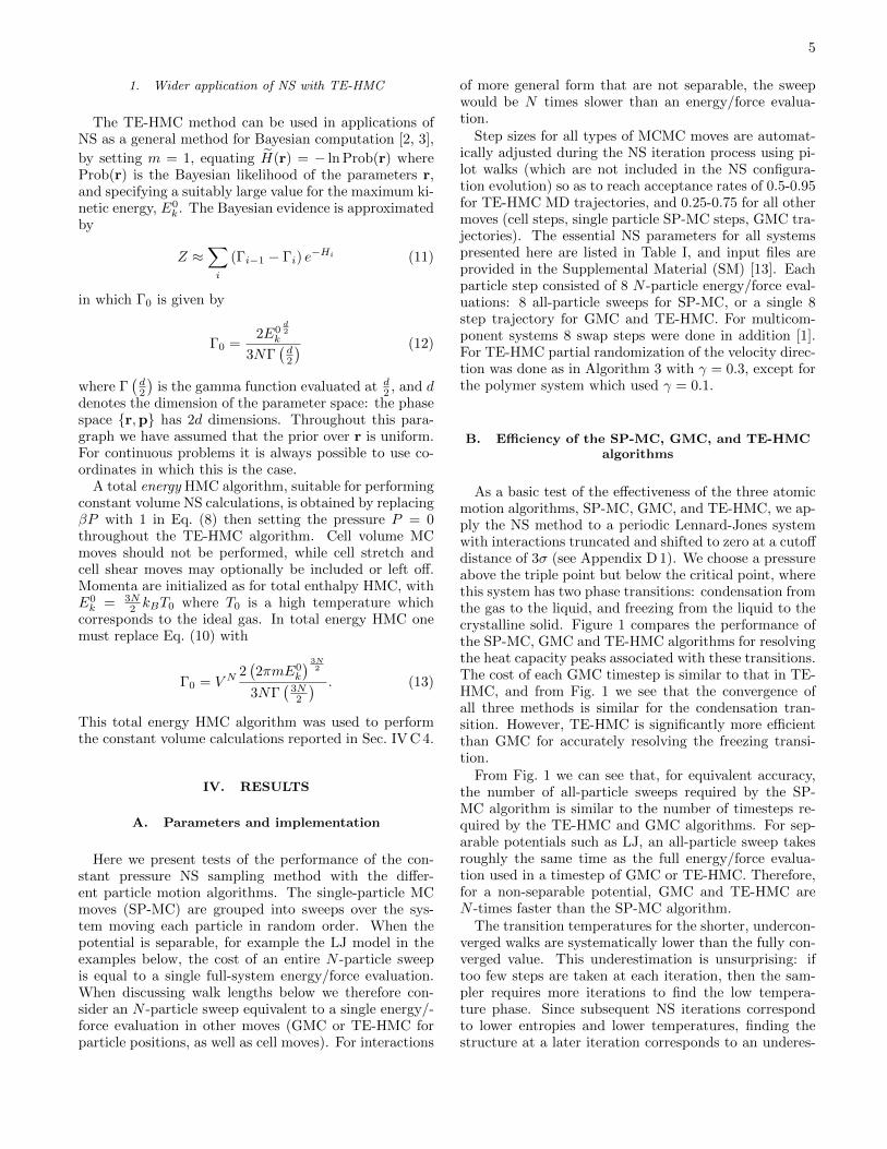
As a basic test of the effectiveness of the three atomicmotion algorithms, SP-MC, GMC, and TE-HMC, we ap-ply the NS method to a periodic Lennard-Jones systemwith interactions truncated and shifted to zero at a cutoffdistance of 3σ (see Appendix D 1). We choose a pressureabove the triple point but below the critical point, wherethis system has two phase transitions: condensation fromthe gas to the liquid, and freezing from the liquid to thecrystalline solid. Figure 1 compares the performance ofthe SP-MC, GMC and TE-HMC algorithms for resolvingthe heat capacity peaks associated with these transitions.The cost of each GMC timestep is similar to that in TE-HMC, and from Fig. 1 we see that the convergence ofall three methods is similar for the condensation tran-sition. However, TE-HMC is significantly more efficientthan GMC for accurately resolving the freezing transi-tion.

From Fig. 1 we can see that, for equivalent accuracy,the number of all-particle sweeps required by the SP-MC algorithm is similar to the number of timesteps re-quired by the TE-HMC and GMC algorithms. For sep-arable potentials such as LJ, an all-particle sweep takesroughly the same time as the full energy/force evalua-tion used in a timestep of GMC or TE-HMC. Therefore,for a non-separable potential, GMC and TE-HMC areN -times faster than the SP-MC algorithm.

The transition temperatures for the shorter, undercon-verged walks are systematically lower than the fully con-verged value. This underestimation is unsurprising: iftoo few steps are taken at each iteration, then the sam-pler requires more iterations to find the low tempera-ture phase. Since subsequent NS iterations correspondto lower entropies and lower temperatures, finding thestructure at a later iteration corresponds to an underes-

6

TABLE I. Parameters for NS runs: pressure P , number of particles N , number of configurations K, number of configurationsremoved per iteration Kr, walk length (all-particle energy/force calls) L, step ratios (particle : cell volume : cell shear : cellstretch [: swap]), minimum temperature Tmin, and number of NS iterations niter. Each particle step consisted of 8 N -particleenergy/force evaluations: 8 all-particle sweeps for SP-MC, or a single 8 step trajectory for GMC and TE-HMC.

P N K Kr L step ratios Tmin niter/106

mono LJ walk length 3.162× 10−2 ε/σ3 64 2304 1 80-2560 1:16:8:8 0.43 ε 2

binary LJ order-disorder 3.162× 10−2 ε/σ3 64 4608 2 1536 1:16:8:8:8 0.043 ε 3

Cu, Au 0.1 GPa 64 2304 1 768 1:16:8:8:8 600 K 2

CuxAu1−x x = [0.25, 0.5, 0.75] 0.1 GPa 64 4608 2 768 1:16:8:8:8 600 K 2

mW water 1.6 MPa 64 1920 1 3168 3:8:4:4 150 K 2

single chain polymer const. V 15 2304 1 5120 1:0:0:0 0.01 ε 1

multichain polymer cluster const. V 8× 15 4608 1 5120 1:0:0:0 0.3 ε 8

multichain polymer 2.3× 10−3 ε/σ3 8× 15 4608 1 5120 1:4:4:4 1.2 ε 3

timated transition temperature. The root mean square(rms) scatter in peak positions shown in Fig. 1 does notgo to zero for any of the methods, even with the longestwalks used (L = 2560 energy/force evaluations): for infi-nite walk lengths, the accuracy is limited by the numberof walkers, K, and the number removed at each iteration,Kr.

C. Example applications

In this section we demonstrate the utility of NS byapplying it to study four diverse systems: the order-disorder transition of a binary LJ alloy, the eutectic ofa copper-gold alloy, the density anomaly of water whichforms open crystal structures, and the phase behaviorof a bead-spring polymer model. In all four cases weuse TE-HMC to explore the position degrees of freedomsince it is most efficient for this range of system sizes,as discussed below in Sec. IV D. All simulations withthe exception of the binary LJ were carried out with theLAMMPS package [9].

1. Order disorder transition

In addition to the condensation, freezing, and marten-sitic transitions that have previously been simulated us-ing NS [1], multicomponent solids also show transitionsrelated to chemical ordering. Here we use NS to simu-late the order-disorder transition of a model binary LJalloy. The potential energy function used, which favorsthe mixing of atoms, is given in Appendix D 2.

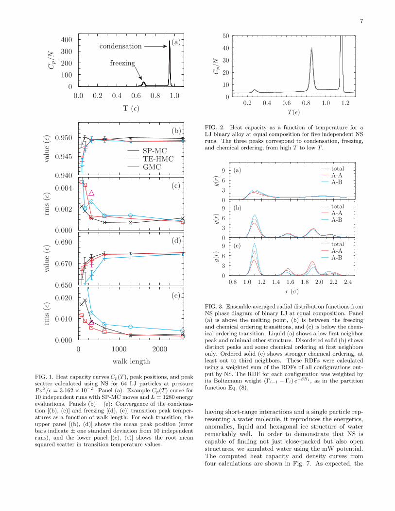
Figure 2 shows the heat capacity curve of this sys-tem. The condensation, freezing and order-disorder tran-sitions can be seen as three separate peaks. Chemicalordering of the alloy can be observed in Figs. 3 and 4which respectively show ensemble averaged radial distri-bution functions (RDFs) and typical configurations ofthe alloy at temperatures corresponding to the orderedand disordered solids, as well as the liquid. Both the

RDFs (Fig. 3) and the representative atomic configura-tions (Fig. 4) show that that at T = 0.95, the system isa liquid, while at T = 0.34 the system is a chemically-disordered close-packed crystal, and at T = 0.17 the crys-tal is chemically ordered.

2. Copper-gold eutectic

A eutectic, where the melting point of a multicompo-nent alloy is reduced at intermediate compositions dueto entropic effects, is an important example of the in-terplay between energy and entropy affecting a phasetransition. We used NS to compute the heat capacity ofCuxAu1−x at a pressure of 0.1 GPa with interactions de-scribed by a simple Finnis-Sinclair type embedded atommodel (FS-EAM) inter-particle potential [14–16] (see Ap-pendix D 3). In Fig. 5 we show the heat capacity Cp(T )for a number of composition values x at a temperaturerange near the melting point, and in Fig. 6 we comparethe resulting computed melting points to experimentalresults from Ref. [17].

We find that the FS-EAM potential gives a meltingtemperature Tm ≈ 1300 K for pure Cu and Tm ≈ 1240 Kfor pure Au. The computed melting temperature is lowerat all intermediate compositions, with a minimum valuein the range 1175-1190 K between 25% and 50% Cu; thecomputed melting temperatures at these two composi-tions are equal to within the error bars of the calcula-tion. While this FS-EAM potential underestimates theexperimental melting points of the two endpoints, moreseverely so for Au (by 8%), nested sampling shows thatit reproduces the qualitative features of a eutectic.

3. Density anomaly of water

The mW potential [18] is a coarse-grained model ofwater, designed to mimic its hydrogen bonded structurethrough a non-bonding angular term, which biases themodel towards tetrahedral coordination. Despite only

7

(e)

0 1000 2000

walk length

0.000

0.010

0.020

rms(ǫ)

(d)

0.650

0.670

0.690

value(ǫ)

(c)

0.000

0.002

0.004

rms(ǫ)

(b)

0.940

0.945

0.950

value(ǫ)

SP-MCTE-HMCGMC

condensation

freezing

(a)

0.0 0.2 0.4 0.6 0.8 1.0

T (ǫ)

0

100

200

300

400

Cp/N

FIG. 1. Heat capacity curves Cp(T ), peak positions, and peakscatter calculated using NS for 64 LJ particles at pressurePσ3/ε = 3.162 × 10−2. Panel (a): Example Cp(T ) curve for10 independent runs with SP-MC moves and L = 1280 energyevaluations. Panels (b) – (e): Convergence of the condensa-tion [(b), (c)] and freezing [(d), (e)] transition peak temper-atures as a function of walk length. For each transition, theupper panel [(b), (d)] shows the mean peak position (errorbars indicate ± one standard deviation from 10 independentruns), and the lower panel [(c), (e)] shows the root meansquared scatter in transition temperature values.

0.2 0.4 0.6 0.8 1.0 1.2

T (ǫ)

0

10

20

30

40

50

Cp/N

FIG. 2. Heat capacity as a function of temperature for aLJ binary alloy at equal composition for five independent NSruns. The three peaks correspond to condensation, freezing,and chemical ordering, from high T to low T .

(c)

0.8 1.0 1.2 1.4 1.6 1.8 2.0 2.2 2.4

r (σ)

0

3

6

9

g(r)

totalA-AA-B

(b)

0

3

6

9g(r)

totalA-AA-B

(a)

0

3

6

9

g(r)

totalA-AA-B

FIG. 3. Ensemble-averaged radial distribution functions fromNS phase diagram of binary LJ at equal composition. Panel(a) is above the melting point, (b) is between the freezingand chemical ordering transitions, and (c) is below the chem-ical ordering transition. Liquid (a) shows a low first neighborpeak and minimal other structure. Disordered solid (b) showsdistinct peaks and some chemical ordering at first neighborsonly. Ordered solid (c) shows stronger chemical ordering, atleast out to third neighbors. These RDFs were calculatedusing a weighted sum of the RDFs of all configurations out-put by NS. The RDF for each configuration was weighted byits Boltzmann weight (Γi−1 − Γi) e

−βHi , as in the partitionfunction Eq. (8).

having short-range interactions and a single particle rep-resenting a water molecule, it reproduces the energetics,anomalies, liquid and hexagonal ice structure of waterremarkably well. In order to demonstrate that NS iscapable of finding not just close-packed but also openstructures, we simulated water using the mW potential.The computed heat capacity and density curves fromfour calculations are shown in Fig. 7. As expected, the

8

FIG. 4. Visualizations of typical configurations for the liquidphase [T = 0.95, (a)], chemically disordered solid [T = 0.34,(b)], and chemically ordered solid [T = 0.17, (c)].

particles were observed to form a hexagonal ice struc-ture, also shown in Fig. 7. By averaging the resultsfrom these calculations, we calculated the freezing tem-perature to be 274.3 ± 1.0 K, the density of ice to be0.9792 ± 0.0005 g/cm

3, and the density of the liquid at

298 K to be 0.9966± 0.0004 g/cm3. All these results are

in excellent agreement with values previously calculatedfor the mW water model: 274.6 K, 0.978 g/cm

3, and

0.997 g/cm3, respectively [18, 19]. We found the maxi-

mum density of water to be 0.9992 ± 0.0002 g/cm3

at atemperature 8.1± 0.3 K above the freezing temperature.

4. Molecular solids

Molecular materials are another system where nestedsampling can be used to efficiently sample the configu-ration space. Both single-molecule systems and multi-molecule systems, such as aggregating proteins or poly-mer melts, are of interest. In previous studies Wang-Landau sampling was used to map the phase behavior ofsingle polymer chains with different lengths [20, 21] andbending stiffnesses [22, 23]. Here we present results fora bead-spring polymer model (see Appendix D 4) with aharmonic bond and cosine angle potential parameterizedby stiffnesses kb and ka, respectively, and a non-bondedLJ interaction with energy ε. This model has been usedto study crystallization in polymers [24], and is similar tothe model used in a previous Wang-Landau study [20].

Figure 8 shows heat capacity curves calculated forthree different systems: (i) a single, fully flexible(ka = 0) bead-spring polymer chain of 15 beads ina constant-volume periodic box with monomer density

2.5 × 10−5σ−3 ≈(

140σ

)3; (ii) 8 fully flexible 15-bead

chains in a constant-volume periodic box with monomer

density 2 × 10−3σ−3 ≈(

18σ

)3; (iii) 8 15-bead chains

with angle stiffness ka = 10ε at fixed pressure P =2.3 × 10−3ε/σ3, and flexible periodic boundary condi-tions. The low monomer densities of the constant-volumesystems do not allow for a single chain to interact withitself through the periodic boundary at the temperaturesof interest. Snapshots of configurations for each systemtype are also shown, illustrating the observed phase tran-

(a)

0

10−3 x = 0

(b)

0

10−3 x = 0.25

(c)

0

10−3

Cp/N

(eV/K

)

x = 0.5

(d)

0

10−3 x = 0.75

(e)

1000 1200 1400

T (K)

0

10−3 x = 1

FIG. 5. Heat capacity as a function of temperature Cp(T ) ofCuxAu1−x for a range of compositions, from pure Au x = 0[panel (a)] to pure Cu x = 1 [panel (e)] in 25% intervals, show-ing variation of melting point peak. Each curve correspondsto an independent NS calculation.

0 25 50 75 100

% Cu

1200

1250

1300

1350

peakT

value(K

) FS-EAM NSexper.

FIG. 6. Melting point as a function of composition in binaryFS-EAM CuxAu1−x [14–16], calculated using the TE-HMCNS algorithm. Experimental values taken from [17]. Eutecticsuppression of the melting point is observed at intermediatecompositions.

9

0.99

0.995

1

DensityCp (scaled to fit)

= 1.6 MPaP

240 260 280 300 320

3 )D

ensi

ty (g

/cm

0.99 0.995

1

T (K)

0.98

0.985

0.975

1.005

1.01

FIG. 7. Heat capacity Cp (in arbitrary units) and densitycurves for 64 mW water particles at a pressure of 1.6 MPa,calculated using the TE-HMC NS algorithm. The inset showsa visualization of the hexagonal ice structure found by NS.Dashed lines in the inset represent the hydrogen-bond net-work.

sitions.

The single chain shows a broad transition below T =0.5 ε, from an extended state to a collapsed, orderedstate, in agreement with previous results [20]. For short,unentangled polymer chains nested sampling leads toslightly lower relative error in the peak height when com-pared to previous results at approximately half the com-putational cost [20, 23]. The constant-volume multichainsystem has two transitions: first, chain aggregation oc-curs at T = 1.4 ε, and second, at T = 0.4 ε the monomersorder, forming a solid cluster with high-symmetry. Thisis reminiscent of the N = 100 single-chain transition ob-served previously [20]. The multichain periodic systemhas two transitions, the first at T = 2.05 ε from a polymergas to a melt, and the second at T = 1.45 ε from a meltto a crystalline solid, in agreement with MD simulationsof polymer crystal nucleation [24].

D. System size dependence of enthalpy distribution

As mentioned in Sec. III A, nested sampling usingGMC creates a series of probability distributions (3) thatcorrespond to uniform distributions in the Cartesian par-

ticle coordinates, r, such that H(r) < Hsup. In this case

Prob(H) is proportional to the density of states for H,which is strictly unimodal. In contrast, TE-HMC worksby performing nested sampling in total phase space, andsamples from a series of probability distributions (6) thatcorrespond to uniform distributions in the phase spacecoordinates (r,p), with H(r,p) < Hsup. In TE-HMC,the marginal distribution for r is not a uniform distribu-tion, and for larger system sizes a bimodality is observed

(a)

(b)

(c)

FIG. 8. Heat capacity per coarse-grained bead Cp/N or Cv/Ncurves for a single bead-spring polymer chain of 15 beads

with monomer density 2.5 × 10−5σ−3 ≈(

140σ

)3[panel (a)],

8 15-bead chains in a periodic box with monomer density

2 × 10−3σ−3 ≈(

18σ

)3[panel (b)], and 8 15-bead chains in a

periodic box with cell moves and P = 2.3 × 10−3ε/σ3 [panel(c)]. Both constant-volume systems use fully flexible (ka =0) models, while the constant pressure system (bottom) haska = 10ε. Snapshots show example polymer conformationscorresponding to the different phases.

in the probability distribution for H at phase transitions.Figure 9 compares the observed probability distribu-

tions for H in the region of the freezing transition (for thesame pressure as the system presented in Sec. IV B) withthe TE-HMC and GMC algorithms, for simulations of 64particles (as used in the earlier subsection) and also for

256 particles. Using TE-HMC for 64 particles Prob(H)is unimodal and broadens slightly at the freezing tran-sition, but never becomes bimodal. For the larger 256

10

(c)

-6.25 -5.75

H (ǫ/atom)

0

50

100

n(H

)

(d)

-6.25 -5.75

H (ǫ/atom)

(a)

0

2000

4000n(H

)(b)

FIG. 9. Distribution of configurational enthalpy (excludingkinetic energy contribution for TE-HMC) for a 64 atom sys-tem [left column (a), (c)] and 256 atom system [right column(b), (d)] of monatomic LJ, for a range of NS iterations thatspans the highest weight configurations for the freezing tran-sition at T ∼ 0.65 ε. Top row [(a), (b)] shows GMC resultsand bottom row [(c), (d)] shows TE-HMC. Colors indicat-ing iteration, from earliest (highest energy) to latest (lowestenergy) are red, yellow, and blue.

particle system, Prob(H) becomes bimodal, which canbe clearly seen in the middle curve (yellow).

In order to obtain an accurate estimate of the inte-grated density of states, Γ(H), TE-HMC must draw asample from the uniform distribution in (r,p), Eq. (6),at each iteration. NS approaches each transition from

above, and if Prob(H) is bimodal, initially all K config-

urations will be in the mode at higher H. To draw a

proper sample from Prob(H) at the phase transition, theMCMC walk must be long enough that the configurationcan feasibly pass back and forth between the two modes,

traversing the intermediate range of H, several times. For

larger N , as Prob(H) gets smaller in the region betweenthe modes, transitions between the two modes will be-come less frequent and much longer MCMC trajectorieswill be required at iterations close to the phase transition.

We observed in Sec. IV B that, for simulations of 64particles, TE-HMC is significantly more efficient thanGMC for accurately resolving the freezing transition.

However, as a result of the bimodality in Prob(H), GMCmay become more efficient than TE-HMC for larger sys-tem sizes. In the future, it would be desirable to developalgorithms which, like TE-HMC, use atomic forces at ev-ery step to expedite configuration space exploration, yet

avoid this bimodality in Prob(H) at larger system sizes.

V. CONCLUSIONS

In this paper we have proposed efficient all-particlemoves using inter-particle forces and dynamics for con-stant pressure nested sampling. The TE-HMC, GMCand SP-MC algorithms reach the same accuracy usingapproximately the same number of full system energy

evaluations (TE-HMC and GMC) or full SP-MC sweeps.For separable potentials, where a single particle move canbe computed in 1/N the cost of a full system energy eval-uation, this makes the three methods equally efficient;for non-separable potentials, where such efficient singleatom moves are not possible, the TE-HMC and GMCalgorithms are N times faster.

The TE-HMC algorithm uses constant energy molec-ular dynamics, implemented in many software packages,but requires extending the NS method to sample posi-tions and momenta, and leads to increasingly bimodalconfigurational enthalpy distributions as the system sizeincreases. This bimodality is likely to make equilibra-tion and sampling difficult for sufficiently large systems,although this has not been a practical problem for the64-120 particle systems we have considered here. TheGMC algorithm, although somewhat less efficient in thissize range, maintains the unimodal configurational en-thalpy distribution of the previous Gibbs-sampling-basedapproach, and is therefore not expected to suffer from abreakdown in ergodicity for larger systems.

We have implemented the constant pressure NSmethod using these algorithms in the pymatnest soft-ware [8], which includes a parallel algorithm and a link tothe LAMMPS package which itself has many inter-particlepotentials available. Using this implementation we haveshown that the constant pressure NS method with thesealgorithms can be used to simulate a wide range of sys-tems with different interaction potentials and types ofphase transitions: order-disorder transitions in binaryLJ, eutectic composition dependence of the melting pointin Cu-Au, freezing of water which has a density anomalyand an open crystal structure, and condensation and so-lidification of a bead-spring polymer model.

ACKNOWLEDGMENTS

R.J.N.B. acknowledges support from EPSRC GrantNo. EP/J017639/1. G.C. acknowledges support fromEPSRC under Grants No. EP/P022596/1 and No.EP/J010847/1. L.B.P. acknowledges support from theRoyal Society. The work of N. B. was supported bythe Office of Naval Research through the U. S. NavalResearch Laboratory’s 6.1 base program. K. M. S. wassupported by the National Research Council’s ResearchAssociateship Program at the U. S. Naval Research Lab-oratory. N.B. and K.M.S. acknowledge computationalresources from the DOD High Performance ComputingModernization Program Office (HPCMPO) at the ARLand AFRL DSRCs.

Appendix A: NS stopping criteria: temperatureestimates

The simplest criteria for stopping the NS iteration areto use a fixed number of iterations (i.e. fixed reduction in

11

entropy) or a fixed potential energy minimum (e.g. closeto the ground state). A more physically appealing crite-rion takes advantage of the approximate correspondencebetween the downward scan in enthalpy and decreasingtemperature. The estimate we use to terminate the out-ermost NS iteration loop is based on the expressions forthermodynamic quantities, such as the partition function(or enthalpy or heat capacity, which are its derivatives).We find that the range of iterations that contribute withsignificant weight to the ensemble average at each tem-perature is sharply peaked. When the contribution ofthe current iteration to the partition function at a spec-ified temperature Tmin is a factor of e10 lower than themaximum contribution of any previous iteration, we as-sume that no later iteration will contribute significantly,and therefore consider the calculation to be convergedfor all T ≥ Tmin. We use this stopping criterion in allsimulations reported here. Note that a monotonic rela-tionship between iteration and temperature is not alwayssatisfied; near phase transitions the dependence is morecomplicated, and setting Tmin too near a phase transitionwill lead to unpredictable behavior.

The convergence criterion described above is efficientenough to evaluate at each iteration for a single choiceof Tmin, but too computationally expensive to use as anestimate of the “current temperature” during NS itera-tions, because it would need to be evaluated for manyvalues of T to find the lowest. We therefore use an in-dependent estimate of the temperature to monitor theprogress of the NS iterations. This estimate is based on

the rate of decrease of Hsup (or Hsup) as a function ofiteration number. The iteration number i is linearly re-lated to the logarithm of configuration space volume (i.e.microcanonical entropy S), and that rate of decrease is

therefore related to ∂H/∂S. The current temperatureduring the NS simulation can be estimated from the fi-nite difference expression

T ≈

(kB

D lnα

Hsup(i−D)− Hsup(i)

)−1

(A1)

where D is an interval over which the finite differenceis taken (1000 iterations here), and kB is Boltzmann’sconstant. We use this expression to monitor the progressof the NS iterations, but not to terminate.

Appendix B: Parallelization

The pymatnest software [8], in which these algorithmsare implemented, combines two separate forms of par-allelization which were previously reported separately.In [1], during step 2 of the NS algorithm, rather thandecorrellating a single cloned configuration alone usinga MCMC walk comprising L energy evaluations, the au-thors evolve np configurations (including the cloned con-figuration) in parallel using np processes through L/npMC moves each. Each configuration is evolved for an

average of np iterations before being recorded and re-moved. Thus the user specifies the average number ofenergy evaluations used to decorrellate a cloned configu-ration from its starting coordinates. In [25, 26], on theother hand, the authors evolve each cloned configurationfor exactly L steps, but they parallelize over np processesby removing Kr = np > 1 configurations at each NS iter-ation, resulting in Kr cloned configurations that can bewalked in parallel.

In pymatnest, we combine the two formulations byallowing for Kr > 1 and evolving the Kr cloned con-figuration in parallel, but also for the number of paral-lel tasks np > Kr, reducing the walk length required ateach iteration. To optimize load balance, each of the Kr

cloned configurations that must be evolved is assignedto a different parallel task, and all remaining paralleltasks (which would otherwise be idle if np > Kr) walkKe = np−Kr additional randomly chosen configurations.

From the probabilities for a configuration to be re-moved or walked at each NS iteration it is possible tocalculate the distribution of the number of walks eachconfiguration has experienced, and from that the meannumber of times a configuration will be walked beforeit is removed 〈nwalks〉. The general expression for thelength of the walk that must be done at each iteration toachieve an expected total walk length 〈L〉, for arbitraryK, Kr, and Ke is

L′ = 〈L〉/〈nwalks〉 = 〈L〉 Kr

Kr +Ke= 〈L〉Kr

np. (B1)

For each MCMC walk in pymatnest, different movetypes are randomly chosen from the list of possible moveswith predetermined ratios until at least L′ energy evalu-ations have been performed.

To maintain load balance the shortest walk must bea few times longer than the longest possible single step,for example, a single SP-MC sweep or an MD/GMC tra-jectory. Therefore the maximum parallelization, np, thatcan be achieved depends only on the total walk length,L, and number of configurations removed at each itera-tion, Kr, and not on the number of configurations, K.For typical runs we show here, Kr = 1, L ≈ 500− 1000,and the length of each MD trajectory is 8. To keep rea-sonable parallel efficiency we find that L′ must be largerthan about 20, so the maximum np ≈ 25− 50.

1. Qualitative behavior of parallelized NS

The computational cost and accuracy of NS depend onthese parameters in a complex way. The total computa-tional work is proportional to K and 〈L〉, and is inde-pendent of Kr and np. If K is increased at fixed Kr, thefraction of configuration space that remains after eachiteration α = (K + 1 − Kr)/(K + 1) comes closer to1.0, and the number of NS iterations required increasesapproximately linearly with K. If instead K and Kr

12

are increased proportionately, α and therefore the num-ber of iterations remain roughly constant, but the workat each iteration (to walk Kr cloned configurations) in-creases proportionately. It is not clear a priori how thenecessary value of 〈L〉 changes with K: there is some ev-idence that once K is large enough, increasing it furtherreduces the distance each cloned configuration must bewalked to decorrelate it sufficiently, but this relationshiprequires further investigation.

The accuracy of the configuration space volume es-timates computed by NS also depends on K and Kr.The value of α determines the resolution in configura-tion space volume, but larger values of K (at constantα) reduce the noise in the estimate (for the same reasonthat the 500th sample out of 999 is a less noisy estima-tor of the median than the 2nd sample out of 3). Thevalue of 〈L〉 also affects the error, because insufficientlywalked configurations have a correlation to the configu-ration they were cloned from, which leads to a deviationfrom the uniform distribution.

Since the useful parallelism is limited by the minimumvalue of L′, which is clearly independent of K, only in-creasing 〈L〉 or Kr can increase it. The former is usefulonly up to the point where the configurations are suffi-ciently decorrelated, as our convergence plots in Sec. IV Bshow. Increasing the latter at constant K decreases theresolution in configuration space volume (by decreasingα), and therefore leads to increased error. Increasing Kr

while also increasing K proportionately maintains theresolution and actually reduces the noise in the config-uration space volumes, but also increases the computa-tional work, but not necessarily the time to solution if npcan also be increased proportionately.

2. Quantitative behavior of parallelized NS

In this section we limit the discussion to the originalconstant pressure, flexible periodic boundary conditionsnested sampling algorithm as implemented by SP-MCand GMC. The same discussion can be extended exactly

to TE-HMC by a change of symbols: H for H and Γ forχ (see Sec. III), so long as one takes care not to confusethe phase space volume Γ and the gamma function in Ap-pendix B 2 a. In the next two subsections we separatelydiscuss the effect of the two approaches to parallelization:first varying Kr while assuming our MCMC draws per-fect samples from the probability distribution (3) [or (6)];second varying Ke at fixed 〈L〉 and Kr.

a. Kr > 1 and Ke = 0

In this subsection, we assume that our MCMC walkyields perfect samples from the distribution (3) (or (6)).

In step 1 of the NS algorithm (see Sec. II) Hsup is up-dated to the lowest of the Kr highest enthalpies in oursample set, and the configuration space volume contained

by the updated Hsup is χi ≈ χ0[(K −Kr + 1)/(K + 1)]i,where i is the NS iteration number. For Kr > 1 it is alsopossible to give analytic estimates of the configurationspace volumes contained by the Kr − 1 higher enthalpy

values between Hsupi−1 and Hsup

i [26]. Thus one may con-sider the configurational entropy contained at fractionalnumbers of NS enthalpy levels.

After a number of enthalpy levels

n∆ =

(K∑

i=K−Kr+1

1

i

)−1

(B2)

the expectation of the logarithm of the configuration

space enclosed by H decreases by 1:

〈lnχi − lnχi+n∆〉 = −1. (B3)

If we assume that it is possible to draw perfect randomsamples from (3) (or (6)), then it can be shown that, afterthe same number of enthalpy levels n∆, the variance of∆ lnχ = lnχi − lnχi+n∆ is given by

Var(∆ lnχ) =d(K−Kr+1)Γ(z)

dz(K−Kr+1)

∣∣∣∣∣z=1

− d(K+1)Γ(z)

dz(K+1)

∣∣∣∣∣z=1(B4)

where Γ(z) is the gamma function. The standard devia-

tion, [Var(∆ lnχ)]12 , represents the rate at which uncer-

tainty in lnχ accumulates during a nested sampling cal-culation. For a serial calculation (Kr = 1 and Ke = 0),

[Var(∆ lnχ)]12 = 1√

K.

Figure 10 shows how the ratio of [Var(∆ lnχ)]12 for par-

allel and serial NS, R = [Var(∆ lnχ)]12 ÷ 1√

K, depends on

Kr

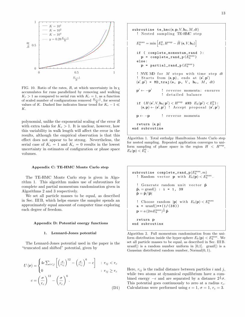
K . R represents the relative rate at which uncertainty inlnχ accumulates during parallel and serial calculations.One can see that lnR converges for K > 102, and forKr

K<∼ 0.25, [Var(∆ lnχ)]

12 ∼ exp

(0.28Kr−1

K

)1√K

. For

larger Kr−1K , R increases more rapidly.

b. Ke > 0 and Kr = 1

Parallelizing with Kr = 1 by using additional tasks towalk Ke > 0 extra configurations (in addition to thosethat were cloned) changes the walk length L from a deter-ministic parameter of the NS method to a stochastic one.It is possible to derive the variance of the walk length

Var(L) = 〈L〉2 Ke

Ke +Kr(B5)

While unlike the case of Kr > 1 there are no analyticresults for the error due to the variability of L, severalobservations can be made. One is that the square rootof the variance (except for the serial case of Ke = 0) isalmost as large as L itself. Another is that the scalingof Var(L) with the number of extra parallel tasks Ke is

13

0 0.5 1

Kr−1K

0

0.5

1

lnR

K = 101

K = 102

K = 104

y = 0.28Kr−1K

FIG. 10. Ratio of the rates, R, at which uncertainty in lnχaccumulates for runs parallelized by removing and walkingKr > 1 as compared to serial run with Kr = 1, as a functionof scaled number of configurations removed Kr−1

K, for several

values of K. Dashed line indicates linear trend for Kr − 1�K.

polynomial, unlike the exponential scaling of the error Rwith extra tasks for Kr > 1. It is unclear, however, howthis variability in walk length will affect the error in theresults, although the empirical observation is that thiseffect does not appear to be strong. Nevertheless, theserial case of Kr = 1 and Ke = 0 results in the lowestuncertainty in estimates of configuration or phase spacevolumes.

Appendix C: TE-HMC Monte Carlo step

The TE-HMC Monte Carlo step is given in Algo-rithm 1. This algorithm makes use of subroutines forcomplete and partial momentum randomization given inAlgorithms 2 and 3 respectively.

We set all particle masses to be equal, as describedin Sec. III B, which helps ensure the sampler spends anapproximately equal amount of computer time exploringeach degree of freedom.

Appendix D: Potential energy functions

1. Lennard-Jones potential

The Lennard-Jones potential used in the paper is the“truncated and shifted” potential, given by

U (r) =

4ε∑i<j

[(σrij

)12

−(σrij

)6

− c]

: rij < rc

0 : rij ≥ rc

c =

(σ

rc

)12

−(σ

rc

)6

.

(D1)

subroutine te_hmc(s,p, V,h0,M, dt)! Nested sampl ing TE−HMC step

Emaxk = min

[E0k, H

sup − H (s, V,h0)]

if ( complete_momentum_rand ):

p = complete_rand_p(Emaxk )

else:

p = partial_rand_p(Emaxk )

! NVE MD f o r M s t e p s with time s t ep dt! S t a r t s from (s,p) , ends at (s′,p′)(s′,p′) = MD_traj(s, p, V , h0, M , dt)

p′ ← −p′ ! r e v e r s e momenta : e n s u r e s! d e t a i l e d ba lance

if (H (s′, V,h0; p′) < Hsup AND Ek(p′) < E0k):

(s,p)← (s′,p′) ! Accept p ropo sa l (s′,p′)

p← −p ! r e v e r s e momenta

return (s,p)end subroutine

Algorithm 1. Total enthalpy Hamiltonian Monte Carlo stepfor nested sampling. Repeated application converges to uni-form sampling of phase space in the region H < Hsup,Ek(p) < E0

k .

subroutine complete_rand_p(Emaxk ,m)

! Random v e c t o r p with Ek(p) < Emaxk .

! Generate random un i t v e c t o r ppi = granf() : i = 1, 3N

p = p/|p|

! Choose random |p| with Ek(p) < Emaxk

a = uranf()**(1/(3N))

p = a (2mEmaxk )

12 p

return pend subroutine

Algorithm 2. Full momentum randomization from the uni-form distribution inside the hyper-sphere Ek(p) < Emax

k . Weset all particle masses to be equal, as described in Sec. III B.uranf() is a random number uniform in [0,1]. granf() is aGaussian distributed random number, Normal(0, 1).

Here, rij is the radial distance between particles i and j,while two atoms at dynamical equilibrium have a com-bined energy −ε and are separated by a distance 2

16σ.

This potential goes continuously to zero at a radius rc.Calculations were performed using ε = 1, σ = 1, rc = 3.

14

subroutine partial_rand_p(p)! P a r t i a l randomizat ion o f momentum p .

! Choose random |p| with Ek(p) < Emaxk

a = uranf()**(1/(3N) )

p = a (2mEmaxk )

12 p/|p|

! i n d i c e s {1, 2, . . . , 3N} i n a random orderrand_indices = random_order (1,3N)

do i = 1, floor(3N/2) ! l oop over p a i r s! p i ck random ang l e from [−γ, γ]θ = urand(−γ, γ)

! p a i r o f components o f p v e c t o rj = rand indices(2i− 1)k = rand indices(2, i)

! 2D r o t a t i o n o f p components j , ku = cos θ pj + sin θ pkv = − sin θ pj + cos θpkpj = upk = v

end do

return pend subroutine

Algorithm 3. Partial momentum randomization for TE-HMCnested sampling. Converges to the uniform distribution insidethe hyper-sphere Ek(p) < Emax

k . We set all particle massesto be equal, as described in Sec. III B. uranf(a, b) is a randomnumber uniform in [a,b]. Note, for odd numbers of atoms N ,we do not rotate p component rand indices(3N). However,since rand indices(3N) is chosen at random, the subroutinepartial rand p satisfies detailed balance.

2. Binary Lennard-Jones alloy potential

The potential used to simulate the binary LennardJones alloy is given by

U (r) =

4∑i<j εij

[(σrij

)12

−(σrij

)6]

: rij < rc

0 : rij ≥ rc(D2)

Calculations were performed using εAA = 1, εAA = 1,εBB = 1.5, σ = 1, rc = 3. In this potential, all atomshave equal atomic radii, but interactions between differ-ent atomic species (A and B) are 1.5 times stronger thanA–A interactions or B–B interactions.

3. CuAu EAM

We used a Finnis-Sinclair type embedded atom model(EAM) for the CuxAu1−x binary alloy. The potential pa-

rameters are from the method in Ref. [14], based on thepure element parameters of Ref. [16], with inter-speciesparameters that are optimized to fit the formation ener-gies of a few crystal structures at selected compositions ofthe binary alloy. The full parameter set for LAMMPS [9]is available for download from Ref. [15].

4. Bead-Spring Polymer Models

The bead-spring models used to study long moleculechains are based on those used by Nguyen et al. to studypolymer crystallization [24]. The energy of a bond be-tween two monomers along the backbone of a polymerchain

Ub(`) =kb2

(`− a)2 (D3)

is harmonic in the distance from the characteristic dis-tance a. The bond stiffness kb = 600ε/σ2. The energy ofan angle θ formed by three consecutive monomers alongthe polymer backbone is given by a cosine potential,

Ua(θ) = ka(1− cos(θ)), (D4)

where the angular stiffness ka penalizes angular devia-tions away from a straight backbone θ = 180o and is seteither to ka = 0 for a fully-flexible chain or to ka = 10ε.The nonbonded interaction between two monomers adistance r from one another is given by Eq. (D1) Themonomer diameter σ = 2−1/6a, so that the bond dis-tance and diameter are commensurate. The cutoff is setto rc = 3σ. As the name suggests, nonbonded interactionsapply only to monomers that are not bonded together.

Appendix E: Minimum cell depth d0

Figure 11 shows the heat capacity of a periodic systemof 64 Lennard-Jones particles at fixed pressure. Thiscalculation used a potential similar to that given inAppendix D 1. In particular, we set the radial cutoffrc = 3σ, and c = 0 in Eq. (D1). We also incorpo-rated the standard long range correction to the energiesto account for interactions beyond the cutoff [27]. Eachcurve corresponds to a single NS simulation, performedusing SP-MC nested sampling, with K = 640, Kr = 1,L = 2824, and MC steps in the ratio (1 64-particle SP-MC sweep : 10 cell volume : 1 cell shear : 1 cell stretch).In these calculations each 64-particle SP-MC sweep wasbroken up into 64 individual single atom SP-MC moves,interspersed between cell moves. In each calculation weconstrained the cell depth to be greater than some min-imum value, d0 (see Eq. (3)). A clear transition to aquasi-2D system is observed when reducing d0. The lo-cation of the condensation transition is independent of d0

for d0 ≥ 0.35, and the location of the freezing transitionfor d0 ≥ 0.65.

15

At low values of d0 the simulation cell becomes verythin in at least one dimension and the system’s behavioris dominated by unphysical correlations introduced bythe periodic boundary conditions. The effect of unphys-ical correlations is reduced at lower densities, and alsoby increasing d0 which constrains the simulation cell tomore cube-like cell shapes. A larger value of d0 is thusrequired at higher densities to sufficiently reduce the un-physical correlations. At the same time, setting d0 tooclose to 1 excludes crystal structures that require a non-cubic simulation cell. Quoting from [1], ‘The window ofindependence from d0 grows wider as the number of par-ticles is increased. For larger numbers of atoms, thereare more ways to arrange those atoms into a given crys-tal structure, including in simulation cells that are closerto a cube. Similarly, unphysical correlations are intro-duced when the absolute number of atoms between facesof the cell becomes too small, and therefore larger simu-lations can tolerate “thinner” simulation cells h0.’ It isclear from Figure 11 that by imposing a suitable mini-mum cell height we can remove the unphysical behaviorfrom the fully flexible cell formulation.

0.5 1 1.5 2

T ∗

10

100

CP

NkB

0.95

0.85

0.75

0.65

0.55

0.45

0.35

0.25

0.15

FIG. 11. Convergence of the heat capacity Cp(T ) with re-spect to minimum cell depth, d0, for a periodic system of 64Lennard-Jones particles at pressure log10 P

∗ = −1.194. Thepeak at high temperature corresponds to condensation, whilethe peak at lower temperature corresponds to freezing. Thelegend on the right shows the value of d0 used in each calcu-lation.

[1] R. J. N. Baldock, L. B. Partay, A. P. Bartok, M. C.Payne, and G. Csanyi, Phys. Rev. B 93, 174108 (2016).

[2] J. Skilling, AIP Conference Proceedings 735, 395 (2004),http://aip.scitation.org/doi/pdf/10.1063/1.1835238.

[3] J. Skilling, J. of Bayesian Analysis 1, 833 (2006).[4] D. Frenkel and B. Smit, “Understanding molecular simu-

lations,” (Academic Press, London, 2002) Chap. III, pp.44–45.

[5] S. Duane, A. Kennedy, B. J. Pendleton, and D. Roweth,Physics Letters B 195, 216 (1987).

[6] J. Skilling, AIP Conference Proceedings 1443, 145(2012).

[7] M. Betancourt, AIP Conference Proceedings 1305, 165(2011).

[8] N. Bernstein, R. J. N. Baldock, L. B. Partay, J. R.Kermode, T. D. Daff, A. P. Bartok, and G. Csanyi, “py-matnest,” https://github.com/libAtoms/pymatnest

(2016).[9] S. Plimpton, Journal of computational physics 117, 1

(1995).[10] L. B. Partay, A. P. Bartok, and G. Csanyi, J. Phys.

Chem. B 114, 10502 (2010).[11] R. L. Smith, Oper. Res. 32, 1296 (1984).[12] L. Lovasz, Math. Program. Ser. A 86, 443 (1999).[13] See, Supplemental Material for pymatnest input files suf-

ficient to reproduce many of the calculations presented inthis paper. x, x (x).

[14] L. Ward, A. Agrawal, K. M. Flores, and W. Windl,(2012), arXiv:1209.0619 [cond-mat.mtrl-sci].

[15] Originally from https://atomistics.osu.edu/eam-

potential-generator/index.php, also available fromthe Supplemental Material [13].

[16] X. W. Zhou, R. A. Johnson, and H. N. G. Wadley, Phys-ical Review B 69, 144113 (2004).

[17] H. Okamoto, D. J. Chakrabarti, D. E. Laughlin, andT. B. Massalski, Bull. Alloy Phase. Diag. 8, 454 (1987).

[18] V. Molinero and E. B. Moore, J. Phys. Chem. B 113,4008 (2009).

[19] D. T. Limmer and D. Chandler, J. Chem. Phys. 135,134503 (2011).

[20] D. T. Seaton, T. Wust, and D. P. Landau, Phys. Rev.E 81, 011802 (2010).

[21] M. P. Taylor, W. Paul, and K. Binder, The Journal ofChemical Physics 131, 114907 (2009).

[22] D. T. Seaton, S. Schnabel, D. P. Landau, and M. Bach-mann, Phys. Rev. Lett. 110, 028103 (2013).

[23] D. T. Seaton, Wang-Landau simulations of thermody-namic behavior in homopolymer systems (University ofGeorgia, 2010).

[24] H. T. Nguyen, T. B. Smith, R. S. Hoy, and N. C.Karayiannis, The Journal of Chemical Physics 143,144901 (2015).

[25] N. S. Burkoff, C. Varnai, S. A. Wells, and D. L. Wild,Biophys. J. 102, 878 (2012).

[26] S. Martiniani, J. D. Stevenson, D. J. Wales, andD. Frenkel, Phys. Rev. X 4, 031034 (2014).

[27] D. Frenkel and B. Smit, “Understanding molecular simu-lations,” (Academic Press, London, 2002) Chap. III, pp.35–37.