ASSESSMENT OF AIR QUALITY IMPACT OF A PROPOSED SECTION OF INTERSTATE 66

by

Wo Ao Carpenter Highway Research Engineer

and

Go Go Clemena Highway Materials Research Analyst

Virginia Highway Research Council (A Cooperative Organization Sponsored Jointly by the Virginia

Department of Highways and the University of Virginia)

Charlottesville, Virginia

March 1972 VHRC 7 I-R24

ASSESSMENT OF AIR. QUALITY IMPACT OF A PROPOSED SECTION OF INTERSTATE 66

W. A. Carpenter Highway Research Engineer

and

G. G. Clemena Highway Materials Research Analyst

INTRODUCTION

This report presents an assessment of the impact of a proposed section of Interstate 66

on the quality of the air in the immediate area of the project and in adjacent areas. The proposed project begins with an extension of existing 1-66 at the interchange on 1-495 in Fairfax County, passes through Arlington County, and terminates near the Key Bridge.

Because of the limited time available for the assessment, consideration was given to only the most abundant gaseous pollutant emitted by motor vehicles, namely, carbon monoxide (CO).

The assessment includes: (1) a mesoscale analysis of the effect of the proposed highway on the total CO emissions for the area, and (2) a microscale or corridor analysis to estimate the CO concentrations to be expected in some immediate areas of the project after its completion.

TRA FFIC DATA

The traffic data used in the analyses were furnished by the Metropolitan Transportation Planning Division of the Virginia Department of Highways. The data were for three years, namely: (1) 1975, the estimated date of completion (EDC); (2) 1985, ten years after the EDC; and (3) 1995, twenty years after the EDCo The data for 1975 were taken as 96% of those for 1985.

The types of traffic data used were: (1) peak hour and off-peak hour conditions in terms of vehicles per hour (vph), average route speed and traffic mix; and (2) daily vehicle miles traveled (DVMT) and traffic mix. Data were furnished for both the proposed 1-66 and the existing major

roads in the area. For the latter, two possibilities were presented: (1) an estimate assuming 1-66 is not built, and (2) an estimate assuming it is.

No data were available for urban mass transit or land use regulations in the area.

The traffic data are summarized in Tables I and II. (All tables and figures are appended.

EMISSION FACTORS (EF)

The vehicular emission factors •or carbon monoxide used in the analyses were developed by the California Division of Highways! •)ased

on the California Air Resources Board (ARB) and the Environmental Protection Agency (EPA) emission control standards.

The emission factors take into account several criteria that affect vehicular emissions: (1) emission control standards for light and heavy duty vehicles for each model year, (2) deterioration of emission control devices as a function of miles traveled, (3) the vehicle model-year mix at any given time, (4) the percentage of heavy duty vehicles (HDV, traffix mix) and (5) emissions as a function of average route speed. It is the consensus of the California ARB and the EPA that emission factors based on the ARB test procedure are realistic for the freeway operating mode, while emission factors based on the 1972 EPA procedures are realistic for the city-street operating mode.

The emission factors have been reviewed and approved by the California ARB and the EPA for use by the California Division of Highways in its air quality impact study. These factors are shown in Figures 1, 2, and 3. It must be emphasized, however, that they probably give slightly lower pollutant concentrations than would be expected in Virginia. This situation arises because California is about three years ahead of the federal standards for automobile pollution control devices. Therefore, in these analyses 1972 emission factors were used for the 1975 study, 1984 factors for the 1985 study, and 1995 factors for the 1995 study.

In the corridor analysis, the projected traffic mix for the proposed 1-66 extension was

approximately 8% HDV. The emission factors for the next higher percentage HDV, namely 10% HDV, were used. This usage would result in approximately 6% higher pollutant concentrations.

ME TE OR OLOG ICAL DATA

The proposed 1-66 extension begins at the interchange on 1-495 in Fairfax County, passes through Arlington County, and terminates near the Key Bridge. Since this general area

is bounded on the west by the Dulles International Airport and on the east by the National Airport, the meteorological data observed for these airports would be ideal for use in the area.

However, because of the inadequacy of the data for Dulles, only the National Airport data were used. Besides, it is felt that the National Airport data are representative of the area under construction.

-2-

The hourly surface meteorological data for National Airport used in this analysis included

the hour of the day, the day of the month, the year, the cloud cover, ceiling height, and wind

direction and speed for the period from January 1952 to December 1961. Ten years data were

used in order to provide valid estimations of the air flow patterns in the study area.

The meteorological data were processed by a computer program whose output is a set

of stability wind rose data which gives the relative frequency distributions of 16 wind directions, 9 wind speed classes, and 6 stability classes for different times and seasons.

(2) The stability wind rose data (Tables III-- VII) were then used in a highway line source dispersion model

(Appendix I) to estimate the pollutant concentration within the highway corridor for 1975 and

1990.

The National Airport meteorological data were obtained from the National Climatic

Center of the National Oceanic and Atmospheric Administration, Asheville, North Carolina.

MATHEMATICAL ANALYSIS

In order to assess the impact of the Interstate 66 on the air quality of the affected area, the meso- and microscale analyses were made as described below.

Mesoscale Analys is

The mesoscale analysis involved estimations of the total carbon monoxide emission

(Appendix II) of the existing and anticipated major roads in the area, with the assumptions that

1-66 is not built and that 1-66 is built. A comparison of such total emission would yield the effect of the proposed 1-66 on the overall air quality of the area. By performing the analysis for the years 1975, 1985, and 1995, one can also estimate the general trend of these pollutant emissions.

The inputs for this analysis were DVMT estimates for each major road and the emission

factors discussed earlier in the report.

The results of the analysis with and without the proposed 1-66 are presented in Table VIII.

The table shows that as the traffic on major roads decreases due to the operation of the proposed 1-66 the emissions from these roads decrease correspondingly. The operation of 1-66 will result

in a reduction in the total CO emissions of 17% for 1975, 7.0% for 1985, and 7.5% for 1995.

Figure 4 illustrates this reduction in CO emissions and shows the general trend of pollutant emissions from 1975 to 1995. The relatively large reductions in emissions (77% without 1-66

and 74% with 1-66) from 1975 to 1985 will be due to more effective emission controls in motor

vehicles.

-3-

Table IX shows, that from 1975 to 1985 there will be a 59% increase in the daily vehicle miles of travel in the area, even-without the proposed 1-66. However, instead of a corresponding increase in CO emissions, there will be a 73% decrease because of improved emission control devices. If 1-66 is built as planned, the CO emissions will be reduced further to 75%. This reduction will result from the combined effects of better emission control devices and the operation of the proposed 1-66. Since emission controls account for 73% of the reduction, the remaining 2% emission reduction must be credited to 1-66o

Microscale Analys is

The microscale analysis produces an estimate of the CO pollutant levels (in ppm. adjacent to the proposed roadway (at 50 ft., 100 ft., and 200 ft. from the edge of the pavement). The analysis was performed for the years 1975 to 1995. As time was very limited for this study, the analysis was carried out only for the winter months (December, January, and February); however,since the worst meteorological conditions and therefore the highest pollutant levels

occur during the winter (see Tables III and IV), this limited analysis provides a valid estimate of the impact of the proposed facility.

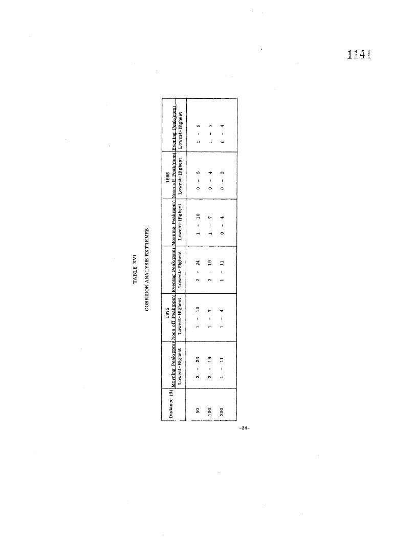
Nine sites were chosen-.as.-.r.epresentative of the corridor area. Figures 5 and 6 show the prevailing and worst CO concentrations, respectively, along site No. 1. The prevailing and worst conditions for all sites are shown in Tables X XV. Note that in some instances the predicted worst case is a lower level than the prevailing case. This implies that because of local conditions (see Appendix I) the theoretically worst case was not as dangerous as others. As explained in Appendix I, all such occurrences are easily understood and it can be shown that in such instances it ts wise to select the prevailing case as also being the worst case.

The extremes for the corridor analyses are summarized in Table XVI. As can be seen

from this table, the low values are well within the federal standards of 35 ppm. averaged over

an hour period. Note that the highest values, although at first alarming, have a very low probability of occurrence (around•,l.-2%) and will last no longer than one hour, thus they will still fall within the federal standards-. (•) (California allows the occurrence of a one-hour peak up to 40 ppmo and 1-66 would be well within this standard°

In summary, the results of this analysis are very encouraging. The values are generally low (recall that the winter months are the most adverse) and the highest values have a very minimal chance of occurrence, Finally, the 1995 predictions show that the highway will have a

minimal effect on the environment.

REFERENCES

lo Ranzier[, A. J., et al., "Motor Vehicle Emission Factors for Estimates of Highway Impact on Air Quality, " California Division of Highways, Research Report No. M & R

657082S-2, February 1972.

2. Environmental Protection Agency, Air Pollution Meteorology, January 1971.

3. Environmental Protection Agency, Federal Register, Volo 36, No. 84, April 30, 1971.

Ranzieri, /•o J., et al0 ,"Meteorology and Its Influence on the Dispersion of Pollutants from

Highway Line Source,-". California Division of Highways, Research Report No. M & R

657082S-3, March 1972.

APPENDIX I

MICROSCA LE ANALYSIS

The microscale analysis- is divided into two categories by meteorological type; i, e., the prevailing and worst•.cases• The worst case, is taken as the light wind condition (4-7 mph) where the winds are parallel to the highway alignment, in which case an accumulation or

build-up effect is observed.

The method used to pred-ict the prevailing nonparallel effect of the roadway is developed in full detail in Reference 4. For the parallel analysis, the Virgina Highway Research Council has developed its own mathematical approach based on the generally accepted Gauss[an dispersion model for gaseous-pollutants. The California model was not used for the parallel analysis since preliminary data:from California indicated that their parallel model may over- estimate by a factor of as much as 1,000%. There is also evidence that the California non-

parallel model occasionally overestimates by as much as 400%• however, since it generally gives accurate results (an occasional overestimation is perhaps more in the public interest than an

underestimation) it was used.

Since the report is not intended as a forum for scientific or mathematical analyses, the Virginia Highway Res.ea•rch Council's parallel model will not be further pursued. However, a complete mathematical presentation is available.

As mentioned in the body of this report, there are some instances where the parallel case does not yield the higher pollutant concentrations. In these instances, it can be seen that

one of several factors has an effect:

1. Pollutants are "trapped" in a cut in the parallel case thus increasing concentrations within the cut, but simultaneously decreasing concentrations outside the cut.

W•nds parallel to a cut or fill prevent the occurrence of aerodynamic eddies near the edges of the protruding level masses and therefore, actually cause a

reduction in local pollutant concentrations.

The roadway may be located near one edge of a large valley (with the observer located at the top of that edge), in which case whads blowing across the valley will pile the pollutants up near the observer while winds parallel to the valley would "'sweep" the pollutants from the hillside.

Again, the theoretical aspects of the gaseous dispersion model have not been detailed; however, detailed descriptions of the analyses can be made available upon request.

APPE NDEK II

MESOSCALE ANALYSIS

The mesoscale analysis evaluates the overall effect of a proposed highway on the air :quality of its environment. A comparison is made of the total emissions with and without the new highway. This comparison indicates the increase or decrease in pollutant emissions that the new facility precipitates by changes in local traffic patterns.

In the analysis the following information is needed:

1o Daily vehicle miles traveled for freeways and local streets both with and without the proposed facility.

2o Average daily route speeds for freeways and local streets.

3. Emission factors for CO as a function of average route speed.

The pollutant emission (tons per day) from each road is estimated from the equation:

Tons per day EoFo XDVMT x1,10 x10 -6

where Eo Fo emission factor in grams/mile DVMT daily vehicle miles traveled

The summation of the emissions from the individual roads yields the total pollutant emission for the affected area.

-10-

TABLE III

RELATIVE FREQUENCY DISTRIBUTION OF STABILITY CLASSES IN WINTER MONTHS

Winter: (December, January, February)

Hours (7, 8, 9) Stability Class

A % Relative Frequenc2

0.4 062

3. 9513

C 7.2378

D 60.9675

E 13.3678

14. 0694

Hours (ii, 12, 13) A 0.4799

B 7. 5305

C 19.3060

D 72. 6836

F

Hours (16, 17, 18) A 0.2216

B 2. 0679

4. 9852

D 62. 2230

17.3929

F 13.1093

-11-

TABLE IV

RELATIVE FREQUENCY DISTRIBUTION OF STABILITY CLASSES IN SUMMER MONTHS

Summer (June, July, August)

Hours (6, 7, *) Stability Class

A % Relative Frequenc•v

19. 0217

B 23. 5145

C 18.1884

D 25.0000

E 6.1232

F 8.1522

Hours (10, 11, 12) A 12.7536

B 29.6014

35. 4710

D 22.1739

F

Hours (15, 16, 17) A 8.8768

30. 6159

41. 9927

D 18. 5145

E

-12-

•

•ooeoeoeoooooooooo. o

000000000000000000

13

z•

o'

z•

,,•z

I-- Z

E ..J

:E Z

Z

O

3:

Z

z-r-

}f

4f

•

• o •

000000000000000000

000000000000000000

000000000000•00•

14

•000•0000000000000•

10000000000000•000•

1000•00000000•00•

15

-16-

TABLE IX

E FFECTS OF EMISSION CONTROL STANDARDS AND 1-66 ON CARBON MONOXIDE EMISSIONS

Total DVMT W/O 1-66, 1975 3,578,712 miles

1995 5,697,570 miles

% Total DVMT increase from 1975

to 1995 59%

% CO emission reduction from 1975 1995

W/O 1-66

W/ 1-66

73%

75%

-17-

z • o X

o

-18-

-19-

-20-

-21-

-22

-23-

-24-

0

4O

AVERAGE i:•OUYE SPEED-I,,IPH

Figure 1: Emission factors for carbon monoxide vs. average route speed on.freeways 10% HDV

25-

0

I00

I0

6 I0 2O 3O

AVERLGE, ROUTE SPEED

Figure" 2: Emission factors for. carbon monoxxue vs. av.erage route spee•l on city .streets-10% HDV.

26

i0 •.,. :•0 40 ,50 AVEI::•/:,C-:•S i::•OUTE SPEED ki•:"H

Figure 3: Emission factors for carbon monoxide vs. avera.ge

•oute spe•d on city-streets 5% ttDV.

250

200

150

IO0

5O

/without 1-66

with 1-66

\ \

\ \

\

1975 1985 1995

Figure 4.

Year

Estimated total carbon monoxide emissions in the area to be affected by, the proposed 1-66.

25

2O

15

10

Year 1975

Morning and evening peak hours

Noon off-peak hours

5O

Figure 5.

100 150 200

Distance from Roadway (feet)

Most probable CO distribution at Site #1.

250

25

2O

15

10

Year 1975

Morning peak hours

Off-peak hours

Evening peak hours

0 50 100 150 200 250

Distance from Roadway (feet)

Figure 6. Worst possible CO distributions at Site #1.

30-