2006-01-0443

Engine-in-the-Loop Testing for Evaluating Hybrid Propulsion Concepts and Transient Emissions – HMMWV Case Study

Zoran Filipi, Hosam Fathy, Jonathan Hagena, Alexander Knafl, Rahul Ahlawat, Jinming Liu, Dohoy Jung, Dennis Assanis, Huei Peng, Jeffrey Stein

Automotive Research Center, University of Michigan

Copyright © 2006 SAE International

ABSTRACT

This paper describes a test cell setup for concurrent running of a real engine and a vehicle system simulation, and its use for evaluating engine performance when integrated with a conventional and a hybrid electric driveline/vehicle. This engine-in-the-loop (EIL) system uses fast instruments and emission analyzers to investigate how critical in-vehicle transients affect engine system response and transient emissions. Main enablers of the work include the highly dynamic AC electric dynamometer with the accompanying computerized control system and the computationally efficient simulation of the driveline/vehicle system. The latter is developed through systematic energy-based proper modeling that tailors the virtual model to capture critical powertrain transients while running in real time. Coupling the real engine with the virtual driveline/vehicle offers a chance to easily modify vehicle parameters, and even study two different powertrain configurations. In particular, the paper describes the engine-in-the-loop study of a V8, 6L engine coupled to a virtual 4x4 High-Mobility Multipurpose Wheeled Vehicle (HMMWV). The results shed light on critical transients in a conventional powertrain and their effect on NOx and soot emissions. Next, the conventional HMMWV powertrain is replaced with a parallel hybrid electric configuration and two power management strategies are examined. Comparison of the conventional and hybrid propulsion options provides detailed insight into fuel economy – emissions tradeoffs at the vehicle level.

INTRODUCTION

Diesel engines are particularly suited for medium-duty vehicles due to their superior fuel economy, favorable torque and power ratings, and durability. However, major design improvements are necessary for diesel propulsion systems to address the rapid escalation of fuel prices and the tighter emissions standards announced by the EPA for 2007 – 2010. Dual-use and military diesel-powered trucks must additionally meet aggressive fuel economy and emissions targets set forth

by the U.S. army for its fleet. Fuel comprises 70% of the tonnage moved when the army is deployed, and any savings attained through improved fuel economy would be further amplified through the reduction of resources devoted to the transport of supplies [1]. The U.S. military is also focused on reducing vehicle’s thermal and visual signature, and the latter translates into a requirement to reduce soot emissions.

New concepts and technologies, such as hybrid propulsion, are required to achieve breakthroughs in fuel economy. These technologies can also have a beneficial impact on emissions, since they offer greater flexibility in controlling engine operation and generally reduce the total mass of exhaust. However, it may not be possible to realize these potential improvements in hybrid system emissions without carefully including them in system analysis, design, and implementation. In the extreme case of a series hybrid optimized for fuel economy, for instance, the engine could be kept operating near its most efficient point most of the time. This, however, may cause rapid changes of engine speed and load as the engine is taken offline and brought back online. Such rapid swings in engine operation may significantly penalize emissions, especially soot. This type of highly transient engine operation is not as pronounced in conventional powertrains. Hence, an in-depth understanding of the dynamic interactions within a hybrid propulsion system and their effect on transient emissions needs to be fully developed before the low-emission potential of diesel hybrids can be established with a high degree of certainty. Only after this type of insight is obtained can both engine-level and vehicle-level strategies be optimized and coordinated to simultaneously minimize fuel consumption and emissions.

Simulation tools are indispensable for the rapid prediction of vehicle behavior during a typical mission and the evaluation and selection of different propulsion concepts early in the design process [1, 3, 4, 5, 6]. They make it possible to vary and optimize component and subsystem designs for given goals and constraints [7, 8]. However, simulation-based vehicle system design is not

without limitations. Conducting vehicle-level studies over complete driving schedules limits the degree of fidelity that can be afforded within a reasonable computational time frame. For instance, simulating soot formation processes in a diesel engine is prohibitively slow in the context of the systems work, since it requires coupling of sophisticated Computational Fluid Dynamics (CFD) models and chemical kinetics [9, 10]. Therefore, even though state-of-the-art vehicle simulations enable assessing vehicle performance, fuel economy and dynamic response with high confidence, the verification of emissions trends necessitates experimentation. Merging the virtual and real worlds, by combining physical engines with virtual drivelines and vehicles, is perhaps the only way to accurately characterize the influence of system design on performance, fuel economy, and emissions early in the design cycle.

This paper couples the virtual simulation and real experimentation, and introduces a setup that concurrently runs a driveline/vehicle simulation and a real engine in a test cell. Using the virtual driveline/vehicle simulation enables rapid prototyping and optimization of different powertrain configurations, designs, and control systems. Furthermore, by implementing the complete engine system in physical hardware, the setup captures the effect of uncertainties in actuator response on engine dynamic behavior. In principle, this setup falls within the broad category of hardware-in-the-loop (HIL) simulators. HIL simulation is often used to design, test, validate, and calibrate embedded controllers prior to integration with physical systems or sub-systems, such as engine fuel injection systems and automatic transmissions. A commonly used definition describes an HIL simulator as “a device that fools the embedded system into thinking that it's operating with real-world inputs and outputs, in real-time” [11]. Our approach differs from such conventional HIL simulation in two respects. First, our use of HIL simulation is not limited to control design, testing and calibration, but addresses broader objectives of evaluating an integrated powertrain system configuration, system optimization, and power management design. Secondly, the setup immerses a major piece of hardware, namely, a multi-cylinder diesel engine together with its accompanying sub-system controller, in the loop. To emphasize these differences, we use the term engine-in-the-loop (EIL) simulation when describing this work.

Engine- (or powertrain-) in-the loop testing is frequently used in industry, mostly for the design and calibration of transmission and engine controllers [12]. Jason and Moskwa [13], for instance, describe the enhancement of dynamometer bandwidths using the hydrostatic principle for the purpose of system control and diagnostics. Similarly, Fleming et al. describe the development of a powertrain-in-the-loop setup that enables control design and implementation specifically for parallel hybrid electric vehicles [14]. Finally, the Argonne National Laboratory (ANL) is heavily investing in HIL capabilities, and serves as the primary site for technology validation

for the U.S. Department of Energy (DOE). Their focus is on enabling the testing of various components in an emulated vehicle environment [7]. Recent work at the ANL has also utilized HIL simulation to investigate tradeoffs between fuel efficiency and NOx emissions [15]. Optimizing the control of a hybrid vehicle (with CVT) based on an analysis of the time spent at given engine regimes and steady-state emission maps led to a viable solution for reducing NOx [15].

The present work differs from the above EIL-related literature in three important ways. First, this work emphasizes fundamental aspects of transient diesel emissions in the context of hybrid propulsion. Diesel emissions are brought to the forefront of powertrain research by the stringent EPA regulation scheduled to take effect in 2007 and 2010. Recently announced tax incentives for purchases of hybrid vehicles in U.S. are contingent upon meeting or exceeding the Bin 5 emissions targets. We seek a realistic characterization of transient dynamics in hybrid powertrains, and a fundamental understanding of the influence of such transient dynamics on powertrain emissions. Such broad and fundamental objectives dictate specialized instrumentation that can sample engine inputs and outputs, including NOx and soot, in real time at very high rates. Secondly, this work uses EIL simulation not only as a control calibration tool, but also as an integrated system-level methodology for hybrid powertrain design and control. Finally, our focus is on medium-duty diesel engines and trucks, rather than passenger cars. The engine used in this work is a 6L V8 diesel produced by the International Truck and Engine Corporation, and it is coupled to a highly dynamic AC dynamometer in the W. E. Lay Automotive Lab at the University of Michigan. Furthermore, the virtual vehicle used in this work is configured based on the specifications of the military High Mobility Multipurpose Wheeled Vehicle (HMMWV), a 4x4 vehicle with exceptional off-road capabilities.

Four key enablers contribute to the viability and effectiveness of the EIL setup used in this work. First, the exceptional fidelity and bandwidth of the AC electric dynamometer, dyno controller, and associated communication system ensure the accurate coupling of the physical engine with the driveline/vehicle simulation in real time. Secondly, the setup’s state-of-the-art test instruments, including a fast NOx analyzer and a differential mobility particulate spectrometer, make it possible to accurately correlate instantaneous emissions with powertrain transients. Thirdly, the use of proper driveline/vehicle models, generated using energy-based automated model reduction techniques that balance model speed vis-à-vis fidelity, enables real time vehicle simulations. Finally, lead/lag filtering and modified causality in the driveline/vehicle simulation minimize the influence of disturbances, noise, and time delays on the setup’s fidelity and bandwidth.

The objectives of the work are to develop the EIL experimentation capability and use it to study engine system behavior when coupled to conventional and

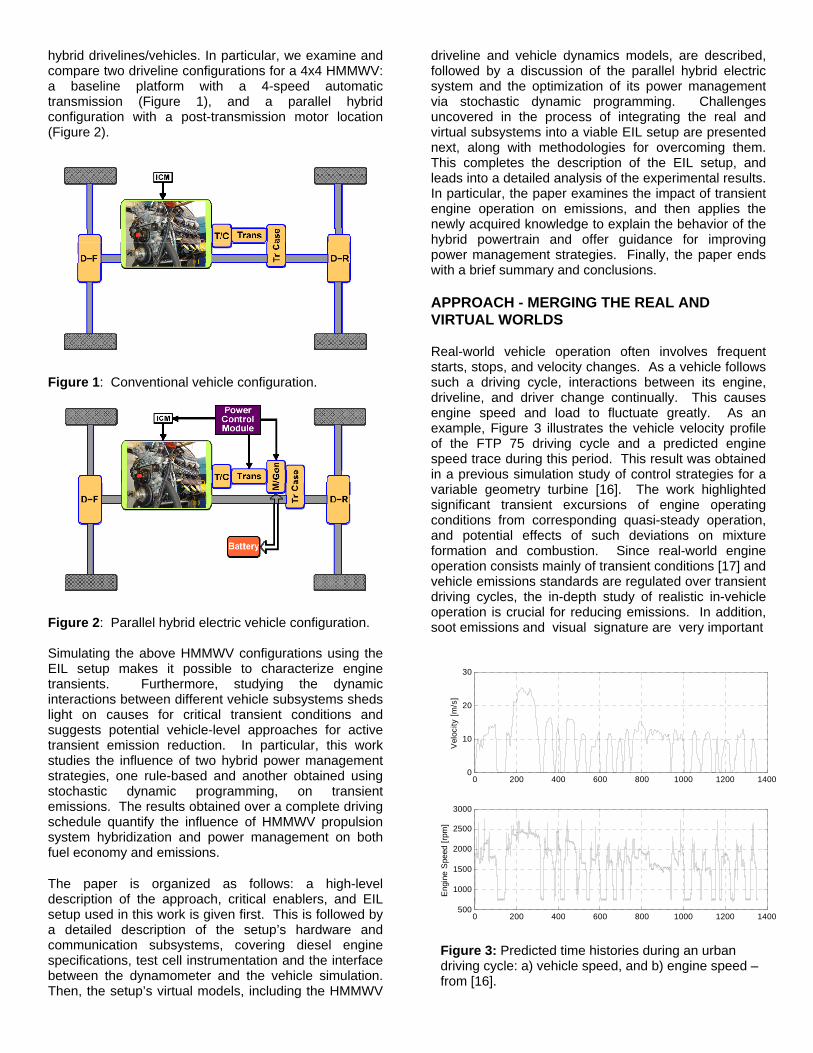
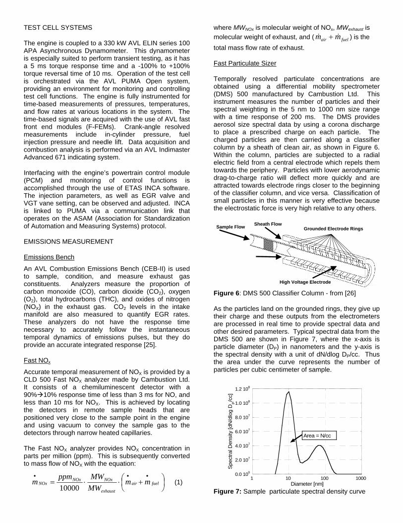
hybrid drivelines/vehicles. In particular, we examine and compare two driveline configurations for a 4x4 HMMWV: a baseline platform with a 4-speed automatic transmission (Figure 1), and a parallel hybrid configuration with a post-transmission motor location (Figure 2).

Figure 1: Conventional vehicle configuration.

Figure 2: Parallel hybrid electric vehicle configuration. Simulating the above HMMWV configurations using the EIL setup makes it possible to characterize engine transients. Furthermore, studying the dynamic interactions between different vehicle subsystems sheds light on causes for critical transient conditions and suggests potential vehicle-level approaches for active transient emission reduction. In particular, this work studies the influence of two hybrid power management strategies, one rule-based and another obtained using stochastic dynamic programming, on transient emissions. The results obtained over a complete driving schedule quantify the influence of HMMWV propulsion system hybridization and power management on both fuel economy and emissions.

The paper is organized as follows: a high-level description of the approach, critical enablers, and EIL setup used in this work is given first. This is followed by a detailed description of the setup’s hardware and communication subsystems, covering diesel engine specifications, test cell instrumentation and the interface between the dynamometer and the vehicle simulation. Then, the setup’s virtual models, including the HMMWV

driveline and vehicle dynamics models, are described, followed by a discussion of the parallel hybrid electric system and the optimization of its power management via stochastic dynamic programming. Challenges uncovered in the process of integrating the real and virtual subsystems into a viable EIL setup are presented next, along with methodologies for overcoming them. This completes the description of the EIL setup, and leads into a detailed analysis of the experimental results. In particular, the paper examines the impact of transient engine operation on emissions, and then applies the newly acquired knowledge to explain the behavior of the hybrid powertrain and offer guidance for improving power management strategies. Finally, the paper ends with a brief summary and conclusions.

APPROACH - MERGING THE REAL AND VIRTUAL WORLDS

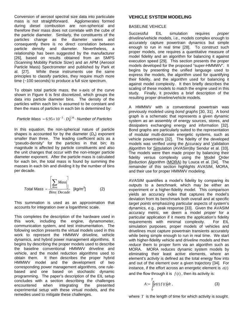
Real-world vehicle operation often involves frequent starts, stops, and velocity changes. As a vehicle follows such a driving cycle, interactions between its engine, driveline, and driver change continually. This causes engine speed and load to fluctuate greatly. As an example, Figure 3 illustrates the vehicle velocity profile of the FTP 75 driving cycle and a predicted engine speed trace during this period. This result was obtained in a previous simulation study of control strategies for a variable geometry turbine [16]. The work highlighted significant transient excursions of engine operating conditions from corresponding quasi-steady operation, and potential effects of such deviations on mixture formation and combustion. Since real-world engine operation consists mainly of transient conditions [17] and vehicle emissions standards are regulated over transient driving cycles, the in-depth study of realistic in-vehicle operation is crucial for reducing emissions. In addition, soot emissions and visual signature are very important

0 200 400 600 800 1000 1200 14000

10

20

30

Vel

ocity

[m/s

]

0 200 400 600 800 1000 1200 1400500

1000

1500

2000

2500

3000

Eng

ine

Spe

ed [r

pm]

Figure 3: Predicted time histories during an urban driving cycle: a) vehicle speed, and b) engine speed – from [16].

in military applications and are closely related to rapid vehicle/engine accelerations [18].

Three methods for investigating in-vehicle engine behavior can be considered:

1. Instrument a vehicle and acquire data as it is driven on open roads.

2. Operate a vehicle on a chassis dynamometer over prescribed driving cycles.

3. Use a dynamometer to couple the engine with virtual dynamic models of the driver, driveline, and vehicle, then run the engine and virtual models concurrently in real time.

While each method has its benefits and drawbacks, option (3) is unique because it eliminates driver and vehicle variability and situates the engine in a test cell, thereby allowing very detailed measurements in a controlled lab environment. Furthermore, it offers the flexibility of easily changing the configuration of the vehicle system and selection of virtual components. Hence, the development of option (3), or engine-in-the-loop methodology, is pursued in this study.

Two pillars of this work are the availability of a suite of vehicle models having appropriate fidelity and the advanced, highly-dynamic dynamometer setup. Both are supported by the ongoing research in the Automotive Research Center (ARC) at the University of Michigan. The main mission of the center is development of advanced models and simulations of ground vehicles, with an emphasis on predictive fully integrated system simulations. Various subsystem models have been integrated in SIMULINK as a common simulation environment to produce a tool for conventional vehicle simulation dubbed Vehicle Engine SIMulation (VESIM) [5]. This platform has subsequently been expanded and utilized for investigating a number of research issues related to hybrid truck propulsion. The fuel economy potential of selected hybrid electric and hydraulic hybrid configurations has been evaluated by

Lin et al. in [6, 19 and 20]. Hierarchical methodologies for optimally designing a complex vehicle system are explored in [8], while [21] considers design under uncertainty. Techniques for optimal power management are addressed in [19, 22]. Finally, a methodology for the combined optimization of hybrid propulsion system design and power management is proposed by Filipi et al. in [23].

In parallel, an advanced test cell, featuring a state-of-the art medium duty diesel engine and a highly dynamic AC dynamometer with the accompanying control system, has been set up for investigations of clean diesel technologies [24]. The dynamometer and test cell hardware vendor (AVL North America) committed to providing the necessary hardware and software for interfacing models in Simulink with the dynamometer and engine controller, thus opening up the possibility of realizing the full benefit of the synergy between modeling and experimental efforts.

The integration of the virtual VESIM components with the hardware in the test cell to create an engine-in-the-loop system is represented schematically in Figure 4. VESIM is used to simulate the vehicle’s driver, driveline, hybrid components, controllers, and vehicle dynamics. VESIM’s forward-looking driveline and vehicle dynamics models make it possible to integrate a virtual driver into the system with the vehicle driving schedule as the only input to the EIL models. The driveline and vehicle developed in VESIM run parallel to the engine in real time to simulate vehicle behavior and provide feedback to the virtual driver and dynamometer controller (EMCON). The engine is coupled to the dynamometer and EMCON, such that its performance depends entirely on signals provided by the driver and response of the virtual vehicle. In case of the hybrid the engine command comes from the power management module rather than directly from the driver. This constitutes a fully integrated EIL setup that emulates the desired vehicle, drivetrain, and driver concurrently in real time.

Simulation (VESIM)Hardware

Vehicle Speed

Driver

Driveline& Vehicle

EMCONController

Dynamometer

T wheel rear

T wheel front

brake

slope front

slope rear

speed

w wheel rear

w wheel front

x front

x rear

VEHICLE DYNAMICS

Rear Road

Front Road

Driving Cycle

w pump

driver demand

w shaft rear

w shaft front

braking_command

T pump

T shaft rear

T shaft front

DRIVETRAIN

vehicle speed

speed set

accel

decel

DRIVER

Load Torque

Driver command

EngineSpeed

DIESEL ENGINE_CNV

0

Constant

DriveCycle

Engine

Figure 4: Engine-in-the-Loop Test Cell Configuration

The highly dynamic AC dynamometer and EMCON 400 flexible test bed controller were delivered by AVL North America. Incorporated within EMCON 400 is ISAC 400, an extension of EMCON that permits the complete simulation of the vehicle configuration, driveline components, driver, and road profile. The ISAC system offers a set of generic submodels that can be used to build a virtual conventional vehicle. More importantly, it also enables linking with a Matlab platform to accept user-defined vehicle, powertrain, and driver models implemented in Simulink. This was the key to fulfilling our objectives, as we were able to generate the entire vehicle and driver in VESIM and attain full flexibility in varying driveline design.

To illustrate the use of the above setup for complete vehicle system simulation, consider a drive cycle at the beginning of which the engine is idling and the vehicle velocity is zero. As the target velocity starts to increase, the virtual driver within VESIM recognizes the difference in demanded and actual vehicle velocities and increases the accelerator pedal position appropriately. This pedal position signal is passed to EMCON and is processed into a signal that is sent to the engine. The engine responds to this signal by producing torque measured by the dynamometer. This torque value is then used as input into the VESIM driveline/vehicle module capable of calculating the impact of the supplied torque on vehicle velocity. The updated vehicle velocity is subsequently translated to engine speed, based on current states in the transmission and torque converter, and this request is sent to the dynamometer through EMCON. The updated vehicle velocity is also provided to the driver, which again compares this value to the driving schedule and determines the pedal position for the following step. When the desired vehicle velocity profile starts to fall, the virtual driver “lifts the foot off the gas pedal” thus making the gas pedal signal zero, and instead sends an appropriate command to a virtual brake model within VESIM. Vehicle velocity changes according to the brake model, and engine speed is commanded appropriately. Thus, the above setup enables the fully integrated simulation of acceleration, coasting, and braking events. Figure 5 represents the exchange of information between VESIM and EMCON. During the experiment, VESIM runs in parallel with the hardware and communicates with EMCON at a frequency of 250 Hz.

Figure 5: Interface between VESIM and EMCON

This completes the high-level description of the EIL setup and its use for integrated vehicle system simulation. Subsequent sections describe the setup’s physical and virtual subsystems in more depth. In particular, the following section describes the engine, dynamometer, dyno controller, and test instrumentation in detail. This is followed by a detailed description of the VESIM-based driveline, vehicle, and hybrid power management models.

EXPERIMENTAL SETUP

ENGINE SPECIFICATIONS

The engine used in this investigation is a 6 L V-8 direct-injection diesel engine manufactured by the International Truck and Engine Corporation. Engine specifications are given in Table 1. The engine is intended for a variety of medium duty truck applications covering the range between Classes IIB and VII. Replacing the standard 6.5 L turbocharged IDI engine developing 145 kW with the more powerful International V8 engine creates a virtual “super-HMMWV”. This is of interest due to the recent emphasis on up-armoring of HMMWV fleets and thus significantly increasing their weight.

The engine incorporates advanced technologies to provide high power density while meeting emissions standards. A hydraulic electric unit injector (HEUI) system permits the precise control of fuel injection timing, pressure, and quantity, and furthermore allows the use of pilot injection. An exhaust gas recirculation (EGR) circuit is used to introduce cooled exhaust gases into the intake manifold in order to decrease NOX emissions. EGR flow rate is controlled through modulation of the EGR valve and the setting of the variable geometry turbocharger (VGT). The VGT is also used to enhance engine performance, as it reduces boost lag and allows control of the intake manifold pressure.

Table 1: Diesel engine specifications

Engine Type DI 4-Stroke Diesel Engine

Configuration V-8, Cam-in-Crankcase 4 Overhead Valves

Bore x Stroke (mm) ( )

95 x 105 Displacement (L) 6.0 Rated Power (kW) 250 @ 3300 rpm Rated Torque (Nm) 760 Compression Ratio 18.0 : 1 Valve Lifters Push Rod-Activated Rocker Arm

Aspiration Variable Geometry Turbine (VGT) / Intercooler

Fuel Delivery System

Generation 2 Hydraulic-Electronic Unit-Injectors (HEUI)

Fuel Specifications US #2 Diesel

VESIM EMCON

Engine Torque

Pedal Position

Dyno Speed

TEST CELL SYSTEMS

The engine is coupled to a 330 kW AVL ELIN series 100 APA Asynchronous Dynamometer. This dynamometer is especially suited to perform transient testing, as it has a 5 ms torque response time and a -100% to +100% torque reversal time of 10 ms. Operation of the test cell is orchestrated via the AVL PUMA Open system, providing an environment for monitoring and controlling test cell functions. The engine is fully instrumented for time-based measurements of pressures, temperatures, and flow rates at various locations in the system. The time-based signals are acquired with the use of AVL fast front end modules (F-FEMs). Crank-angle resolved measurements include in-cylinder pressure, fuel injection pressure and needle lift. Data acquisition and combustion analysis is performed via an AVL Indimaster Advanced 671 indicating system.

Interfacing with the engine’s powertrain control module (PCM) and monitoring of control functions is accomplished through the use of ETAS INCA software. The injection parameters, as well as EGR valve and VGT vane setting, can be observed and adjusted. INCA is linked to PUMA via a communication link that operates on the ASAM (Association for Standardization of Automation and Measuring Systems) protocol.

EMISSIONS MEASUREMENT

Emissions Bench

An AVL Combustion Emissions Bench (CEB-II) is used to sample, condition, and measure exhaust gas constituents. Analyzers measure the proportion of carbon monoxide (CO), carbon dioxide (CO2), oxygen (O2), total hydrocarbons (THC), and oxides of nitrogen (NOX) in the exhaust gas. CO2 levels in the intake manifold are also measured to quantify EGR rates. These analyzers do not have the response time necessary to accurately follow the instantaneous temporal dynamics of emissions pulses, but they do provide an accurate integrated response [25].

Fast NOx

Accurate temporal measurement of NOX is provided by a CLD 500 Fast NOX analyzer made by Cambustion Ltd. It consists of a chemiluminescent detector with a 90% 10% response time of less than 3 ms for NO, and less than 10 ms for NOX. This is achieved by locating the detectors in remote sample heads that are positioned very close to the sample point in the engine and using vacuum to convey the sample gas to the detectors through narrow heated capillaries.

The Fast NOX analyzer provides NOX concentration in parts per million (ppm). This is subsequently converted to mass flow of NOX with the equation:

⎟⎠⎞

⎜⎝⎛ +⋅⋅=

•••

fuelair

exhaust

NOxNOxNOx mm

MWMWppm

m10000

(1)

where MWNOx is molecular weight of NOx, MWexhaust is molecular weight of exhaust, and ( fuelair mm && + ) is the total mass flow rate of exhaust.

Fast Particulate Sizer

Temporally resolved particulate concentrations are obtained using a differential mobility spectrometer (DMS) 500 manufactured by Cambustion Ltd. This instrument measures the number of particles and their spectral weighting in the 5 nm to 1000 nm size range with a time response of 200 ms. The DMS provides aerosol size spectral data by using a corona discharge to place a prescribed charge on each particle. The charged particles are then carried along a classifier column by a sheath of clean air, as shown in Figure 6. Within the column, particles are subjected to a radial electric field from a central electrode which repels them towards the periphery. Particles with lower aerodynamic drag-to-charge ratio will deflect more quickly and are attracted towards electrode rings closer to the beginning of the classifier column, and vice versa. Classification of small particles in this manner is very effective because the electrostatic force is very high relative to any others.

Sample Flow Sheath Flow

High Voltage Electrode

Grounded Electrode Rings

Figure 6: DMS 500 Classifier Column - from [26]

As the particles land on the grounded rings, they give up their charge and these outputs from the electrometers are processed in real time to provide spectral data and other desired parameters. Typical spectral data from the DMS 500 are shown in Figure 7, where the x-axis is particle diameter (DP) in nanometers and the y-axis is the spectral density with a unit of dN/dlog DP/cc. Thus the area under the curve represents the number of particles per cubic centimeter of sample.

0.0 100

2.0 107

4.0 107

6.0 107

8.0 107

1.0 108

1.2 108

1 10 100 1000

Spec

tral D

ensi

ty [d

N/d

log

DP/c

c]

Diameter [nm]

Area = N/cc

Figure 7: Sample particulate spectral density curve

Conversion of aerosol spectral size data into particulate mass is not straightforward. Agglomerates formed during diesel combustion are non-spherical and therefore their mass does not correlate with the cube of the particle diameter. Similarly, the constituents of the particles change as the diameter varies and consequently there is no direct correlation between particle density and diameter. Nevertheless, a relationship has been suggested by the manufacturer [26], based on results obtained from an SMPS (Scanning Mobility Particle Sizer) and an APM (Aerosol Particle Mass) Spectrometer and published by Park et al. [27]. While these instruments use the same principles to classify particles, they require much more time (~100 seconds) to produce a full size spectrum.

To obtain total particle mass, the x-axis of the curve shown in Figure 6 is first discretized, which groups the data into particle diameter bins. The density of the particles within each bin is assumed to be constant and then the mass of particles in each bin is determined by:

Particle Mass ⋅⋅×= − 34.231095.6 PD Number of Particles

In this equation, the non-spherical nature of particle shapes is accounted for by the diameter (Dp) exponent smaller than three. The leading coefficient acts as a “pseudo-density” for the particles in that bin; its magnitude is affected by particle constituents and also the unit changes that occur with the non-integer particle diameter exponent. After the particle mass is calculated for each bin, the total mass is found by summing the masses in each bin and dividing it by the number of bins per decade.

Total Mass DecadeBins

MassBins ⎥

⎥⎦

⎤

⎢⎢⎣

⎡

=∑

[kg/m3] (2)

This summation is used as an approximation that accounts for integration over a logarithmic scale.

This completes the description of the hardware used in this work, including the engine, dynamometer, communication system, and test instrumentation. The following section presents the virtual models used in this work to represent the HMMWV driveline, vehicle dynamics, and hybrid power management algorithms. It begins by describing the proper models used to describe the baseline conventional HMMWV driveline and vehicle, and the model reduction algorithms used to obtain them. It then describes the proper hybrid HMMWV model and the development of two corresponding power management algorithms, one rule-based and one based on stochastic dynamic programming. The paper’s description of the EIL setup concludes with a section describing the challenges encountered when integrating the presented experimental setup with these virtual models, and the remedies used to mitigate these challenges.

VEHICLE SYSTEM MODELING

BASELINE VEHICLE

Successful EIL simulation requires proper driveline/vehicle models, i.e., models complex enough to accurately capture powertrain dynamics but simple enough to run in real time [28]. To construct such proper models, one requires a quantitative measure of model fidelity and an algorithm for balancing it against execution speed [29]. This section presents the proper models developed for the proposed “super-HMMWV”. It begins by presenting the unified language used to express the models, the algorithm used for quantifying their fidelity, and the algorithm used for balancing it against model complexity. It then briefly describes the scaling of these models to match the engine used in this study. Finally, it provides a brief description of the resulting proper driveline/vehicle models.

A HMMWV with a conventional powertrain was previously modeled using bond graphs [30, 31]. A bond graph is a schematic that represents a given dynamic system as an assembly of energy sources, stores, and dissipaters exchanging energy and information [32]. Bond graphs are particularly suited to the representation of modular multi-domain energetic systems, such as vehicle powertrains [32]. The fidelity of the developed models was verified using the Accuracy and Validation Algorithm for Simulation (AVASim)by Sendur et al. [33]. The models were then made proper by balancing their fidelity versus complexity using the Model Order Reduction Algorithm (MORA) by Louca et al. [34]. The remainder of this section highlights AVASIM, MORA, and their use for proper HMMWV modeling.

AVASIM quantifies a model’s fidelity by comparing its outputs to a benchmark, which may be either an experiment or a higher-fidelity model. This comparison yields an accuracy index that captures the model’s deviation from its benchmark both overall and at specific target points emphasizing particular aspects of system’s dynamics, e.g., peak response [33]. Given the AVASIM accuracy metric, we deem a model proper for a particular application if it meets the application’s fidelity requirements with minimal complexity. For EIL simulation purposes, proper models of vehicles and drivelines must capture powertrain transients accurately while being simple enough to run in real time. We start with higher-fidelity vehicle and driveline models and then reduce them to proper form via an algorithm such as MORA. MORA reduces dynamic system models by eliminating their least active elements, where an element’s activity is defined as the total energy flow into and out of the element over a given trajectory [34]. For instance, if the effort across an energetic element is )(te and the flow through it is )(tf , then its activity is:

∫=T

dttfteA0

)()(: , (3)

where T is the length of time for which activity is sought.

The fundamental premise behind MORA is that an energetic element’s activity is indicative of its importance to the model’s fidelity. This premise is supported by both theoretical and computational results [34, 35].

Previous research used MORA in conjunction with AVASIM to construct a proper model of an existing HMMWV [30, 31]. This model’s parameters were then scaled to match the engine used in this case study. In particular, the HMMWV torque converter, gear ratios, shift map, and final drive were scaled to provide desired mobility, smooth shifting, and fuel efficiency, given the speed and torque range of the International V8 engine [36]. The resulting driveline and vehicle parameters are given in Table 2. Furthermore, Figures 8-10 show the bond graphs corresponding to the complete powertrain model, the driveline submodel, and the vehicle submodel, respectively.

Figure 8 is a schematic representation of an entire “super-HMMWV” (from [36]). This representation breaks down the vehicle system into four main subsystems: an engine subsystem, a drive train subsystem, a driver subsystem, and a vehicle subsystem. Full arrows represent information flow, while half arrows represent energy flow. The model’s external inputs include the drive cycle and road profile.

Figure 9 shows the internal layout of the vehicle system model given in Figure 8 (from [36]). The exchange of energy between this model and the driveline is represented by the wheel_hub connector. Some of the wheel hub’s power is stored in the wheel hub inertia, I, dissipated by the wheel bearing resistance, R, or dissipated by the braking resistance, B_brake, which is modulated by an external signal from the driver. The remaining power supplied by the wheel hub is transformed from the rotational mechanical domain to the translational domain by the wheel radius, represented by a modulated transformer, MTF. Some power is lost to slipping resistance (B_slip), rolling resistance (B_rolling), and aerodynamic drag (Raero), but the remaining power is stored in the vehicle’s inertia, represented by MI.

The schematic in Figure 10 breaks down the drivetrain into a torque converter, a transmission, a transmission shift controller, and a final drive. The torque converter is modeled using standard characteristic factor curves, the transmission is modeled as a modulated transformer, shift control is modeled using a simple shift map, and the final drive is modeled as an additional transformer. Further details about the modeling of these components and the modeling of super-HMMWV powertrain dynamics in general are omitted for brevity and provided by other references [30, 31, 36].

The above super-HMMWV models were expressed in the bond graph language SIDOPS and implemented in the modeling tool 20Sim [37]. For EIL simulation, the engine module was removed and the drivetrain was connected to the EMCON interface. The models were

then translated into differential algebraic equations (DAEs) and expressed in the C language. Embedding the C code into Simulink as a Simulink-executable S-function (using Matlab’s external interface C-MEX function) finally allowed the models to be connected to the EMCON interface.

This completes the description of the proper models used for the conventional super-HMMWV in this study. The following section describes the modeling of the parallel electric super-HMMWV and the development of its two power management algorithms.

Table 2: HMMWV driveline and vehicle model parameters; driveline modified to match the high-performance V8 engine.

Drivetrain & Vehicle Specifications

T/C Turbine inertia [kg*m2] 0.2

1st gear ratio [-] 3.42 2nd gear ratio [-] 2.26 3rd gear ratio [-] 1.50 4th gear ratio [-] 1.00 1st Gear efficiency [-] 0.94 2nd Gear efficiency [-] 0.96 3rd Gear efficiency [-] 0.97 4th Gear efficiency [-] 0.97 Differential drive ratio [-] 3.56 Differential efficiency [-] 0.94 Number of wheels [-] 4 Sprung vehicle mass [kg] 4672 Unsprung vehicle mass – Front [kg] 220 Unsprung vehicle mass – Rear [kg] 220 Wheel inertia [kg*m2] 32 Brake viscous damping [N*m*s/rad] 170 Wheel radius [m] 0.4412 Wheel bearing damping [N*m*s/rad] 4.0 Road/tire friction coefficient [-] 0.7 Frontal area [m^2] 3.58 Coefficient of drag [-] 0.7

Engine Drivetrain

Driverfileinput

cycle

Vehicle

Figure 8: System model topology in 20SIM

wheel_hub

Brake

X_outV_out

a_out

kappa_out

F_tire

Mx_in

1

I

B_brake

MTF B_rolling

R

B_slip

R aero

MI

1

0

1

Figure 9: Vehicle Model

shaft

demand

pump Torque Converter Transmission Propshaft/Differential

ShiftLogic

f

Figure 10: Drive Train Model

HYBRID PROPULSION AND POWER MANAGEMENT

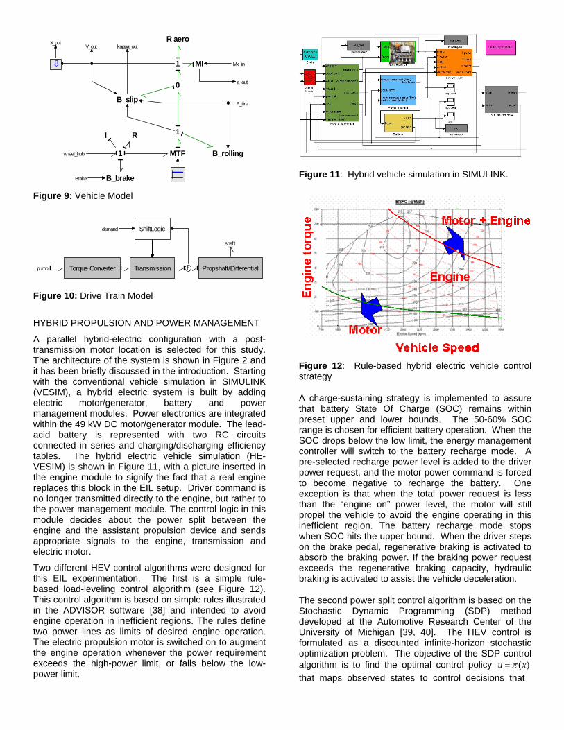
A parallel hybrid-electric configuration with a post-transmission motor location is selected for this study. The architecture of the system is shown in Figure 2 and it has been briefly discussed in the introduction. Starting with the conventional vehicle simulation in SIMULINK (VESIM), a hybrid electric system is built by adding electric motor/generator, battery and power management modules. Power electronics are integrated within the 49 kW DC motor/generator module. The lead-acid battery is represented with two RC circuits connected in series and charging/discharging efficiency tables. The hybrid electric vehicle simulation (HE-VESIM) is shown in Figure 11, with a picture inserted in the engine module to signify the fact that a real engine replaces this block in the EIL setup. Driver command is no longer transmitted directly to the engine, but rather to the power management module. The control logic in this module decides about the power split between the engine and the assistant propulsion device and sends appropriate signals to the engine, transmission and electric motor.

Two different HEV control algorithms were designed for this EIL experimentation. The first is a simple rule-based load-leveling control algorithm (see Figure 12). This control algorithm is based on simple rules illustrated in the ADVISOR software [38] and intended to avoid engine operation in inefficient regions. The rules define two power lines as limits of desired engine operation. The electric propulsion motor is switched on to augment the engine operation whenever the power requirement exceeds the high-power limit, or falls below the low-power limit.

Figure 11: Hybrid vehicle simulation in SIMULINK.

Figure 12: Rule-based hybrid electric vehicle control strategy

A charge-sustaining strategy is implemented to assure that battery State Of Charge (SOC) remains within preset upper and lower bounds. The 50-60% SOC range is chosen for efficient battery operation. When the SOC drops below the low limit, the energy management controller will switch to the battery recharge mode. A pre-selected recharge power level is added to the driver power request, and the motor power command is forced to become negative to recharge the battery. One exception is that when the total power request is less than the “engine on” power level, the motor will still propel the vehicle to avoid the engine operating in this inefficient region. The battery recharge mode stops when SOC hits the upper bound. When the driver steps on the brake pedal, regenerative braking is activated to absorb the braking power. If the braking power request exceeds the regenerative braking capacity, hydraulic braking is activated to assist the vehicle deceleration.

The second power split control algorithm is based on the Stochastic Dynamic Programming (SDP) method developed at the Automotive Research Center of the University of Michigan [39, 40]. The HEV control is formulated as a discounted infinite-horizon stochastic optimization problem. The objective of the SDP control algorithm is to find the optimal control policy ( )u xπ= that maps observed states to control decisions that

minimize the expected total cost over an infinite horizon:

( )1

00

( ) lim , ( )k

Nk

k kN w k

J x E g x xπ γ π−

→∞=

⎧ ⎫= ⎨ ⎬

⎩ ⎭∑ (4)

where g is the instantaneous cost incurred, 0 1γ< < is the discount factor, and 0( )J xπ indicates the resulting expected cost when the system starts at state 0x and follows the policy π thereafter. For our hybrid vehicle control problem, the control signal is engine power eP .

Stochastic dynamic programming problems have been extensively studied in the literature. It has been shown that the algorithm can handle constrained nonlinear optimization problems under uncertainties [41]. In this study, an approximate policy iteration algorithm is used.

For the hybrid electric vehicle problem, the state variables related to the vehicle, engine and battery all evolve according to deterministic dynamic equations. The state variable that is stochastic in nature, thus requiring an SDP solution, is the driver power demand. Driver power demand in realistic situations depends on many factors, such as vehicle and road load, weather, and traffic conditions. Therefore, we hypothesize that defining an SDP problem around a stochastic power demand obtained through the combination of many driving cycles, and subsequently performing the optimization, would result in a control law that is suitable for diverse driving conditions. Since it is not based on a particular driving cycle (time signal), but rather the statistical characteristics of many driving cycles, it is naturally non-cycle-beating. Furthermore, the resulting control algorithm is full-state feedback and thus can be implemented directly as a look-up table.

The SDP problem is solved by a policy iteration algorithm, using Bellman’s optimality equation. The policy iteration conducts a policy evaluation step and a policy improvement step in an iterative manner until the optimal cost function converges. In the policy evaluation step, given a control policy π , we calculate the corresponding cost function ( )J xπ by iteratively updating the Bellman equation

( ){ }1( ) ( , ( )) 's i i i s

wJ x g x x E J xπ ππ γ+ = + (5)

for all i , where s is the iteration number, and 'x is the new state, i.e., ( )' , ( ),i ix f x x wπ= . However, the first

two components of state 'x , ( , )whSOC ω , do not necessarily fall exactly on the state grid. In this case, a linear interpolation of the cost function along the first two dimensions is used. In order to accelerate the computations, only a fixed number of iterations are performed regardless of the convergence of the estimated cost function. This truncated policy-evaluation method has been shown to reduce the computation time effectively [40]. In the policy improvement step, the improved policy is found through the following equation

{ }u ( )

'( ) argmin ( , ) ( ')i

i i

wU xx g x u E J xππ γ

∈

⎡ ⎤= +⎣ ⎦ (6)

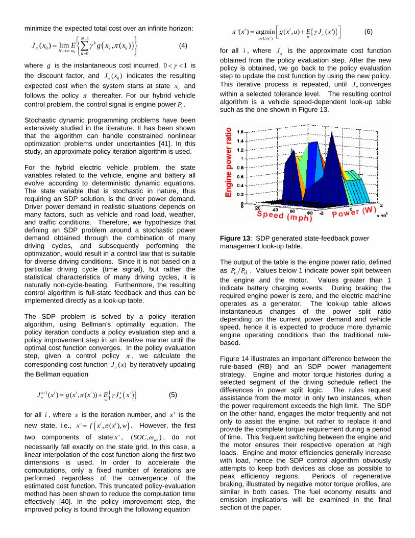
for all i , where Jπ is the approximate cost function obtained from the policy evaluation step. After the new policy is obtained, we go back to the policy evaluation step to update the cost function by using the new policy. This iterative process is repeated, until Jπ converges within a selected tolerance level. The resulting control algorithm is a vehicle speed-dependent look-up table such as the one shown in Figure 13.

Figure 13: SDP generated state-feedback power management look-up table.

The output of the table is the engine power ratio, defined as de PP . Values below 1 indicate power split between the engine and the motor. Values greater than 1 indicate battery charging events. During braking the required engine power is zero, and the electric machine operates as a generator. The look-up table allows instantaneous changes of the power split ratio depending on the current power demand and vehicle speed, hence it is expected to produce more dynamic engine operating conditions than the traditional rule-based.

Figure 14 illustrates an important difference between the rule-based (RB) and an SDP power management strategy. Engine and motor torque histories during a selected segment of the driving schedule reflect the differences in power split logic. The rules request assistance from the motor in only two instances, when the power requirement exceeds the high limit. The SDP on the other hand, engages the motor frequently and not only to assist the engine, but rather to replace it and provide the complete torque requirement during a period of time. This frequent switching between the engine and the motor ensures their respective operation at high loads. Engine and motor efficiencies generally increase with load, hence the SDP control algorithm obviously attempts to keep both devices as close as possible to peak efficiency regions. Periods of regenerative braking, illustrated by negative motor torque profiles, are similar in both cases. The fuel economy results and emission implications will be examined in the final section of the paper.

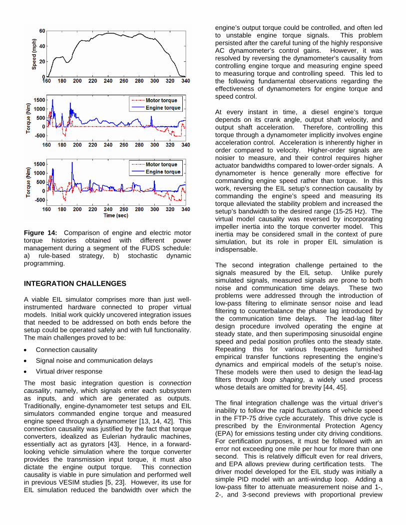
Figure 14: Comparison of engine and electric motor torque histories obtained with different power management during a segment of the FUDS schedule: a) rule-based strategy, b) stochastic dynamic programming.

INTEGRATION CHALLENGES

A viable EIL simulator comprises more than just well-instrumented hardware connected to proper virtual models. Initial work quickly uncovered integration issues that needed to be addressed on both ends before the setup could be operated safely and with full functionality. The main challenges proved to be:

• Connection causality • Signal noise and communication delays • Virtual driver response

The most basic integration question is connection causality, namely, which signals enter each subsystem as inputs, and which are generated as outputs. Traditionally, engine-dynamometer test setups and EIL simulators commanded engine torque and measured engine speed through a dynamometer [13, 14, 42]. This connection causality was justified by the fact that torque converters, idealized as Eulerian hydraulic machines, essentially act as gyrators [43]. Hence, in a forward-looking vehicle simulation where the torque converter provides the transmission input torque, it must also dictate the engine output torque. This connection causality is viable in pure simulation and performed well in previous VESIM studies [5, 23]. However, its use for EIL simulation reduced the bandwidth over which the

engine’s output torque could be controlled, and often led to unstable engine torque signals. This problem persisted after the careful tuning of the highly responsive AC dynamometer’s control gains. However, it was resolved by reversing the dynamometer’s causality from controlling engine torque and measuring engine speed to measuring torque and controlling speed. This led to the following fundamental observations regarding the effectiveness of dynamometers for engine torque and speed control.

At every instant in time, a diesel engine’s torque depends on its crank angle, output shaft velocity, and output shaft acceleration. Therefore, controlling this torque through a dynamometer implicitly involves engine acceleration control. Acceleration is inherently higher in order compared to velocity. Higher-order signals are noisier to measure, and their control requires higher actuator bandwidths compared to lower-order signals. A dynamometer is hence generally more effective for commanding engine speed rather than torque. In this work, reversing the EIL setup’s connection causality by commanding the engine’s speed and measuring its torque alleviated the stability problem and increased the setup’s bandwidth to the desired range (15-25 Hz). The virtual model causality was reversed by incorporating impeller inertia into the torque converter model. This inertia may be considered small in the context of pure simulation, but its role in proper EIL simulation is indispensable.

The second integration challenge pertained to the signals measured by the EIL setup. Unlike purely simulated signals, measured signals are prone to both noise and communication time delays. These two problems were addressed through the introduction of low-pass filtering to eliminate sensor noise and lead filtering to counterbalance the phase lag introduced by the communication time delays. The lead-lag filter design procedure involved operating the engine at steady state, and then superimposing sinusoidal engine speed and pedal position profiles onto the steady state. Repeating this for various frequencies furnished empirical transfer functions representing the engine’s dynamics and empirical models of the setup’s noise. These models were then used to design the lead-lag filters through loop shaping, a widely used process whose details are omitted for brevity [44, 45].

The final integration challenge was the virtual driver’s inability to follow the rapid fluctuations of vehicle speed in the FTP-75 drive cycle accurately. This drive cycle is prescribed by the Environmental Protection Agency (EPA) for emissions testing under city driving conditions. For certification purposes, it must be followed with an error not exceeding one mile per hour for more than one second. This is relatively difficult even for real drivers, and EPA allows preview during certification tests. The driver model developed for the EIL study was initially a simple PID model with an anti-windup loop. Adding a low-pass filter to attenuate measurement noise and 1-, 2-, and 3-second previews with proportional preview

gains proved to be necessary for ensuring desired dynamic performance. The resulting modified driver model is shown in Figure 15.

Desired Speed

Vehicle Speed

+

-

Drive Cycle

Preview

Lead/Lag Filter

Speed Error I Gain

P Gain

+ 1/s +

Anti-windup Gain

+ -

+ +

Preview Gain

+ Pedal Limits

>0

<0

Driver Command

Brake Command

Figure 15: Driver model in SIMULINK

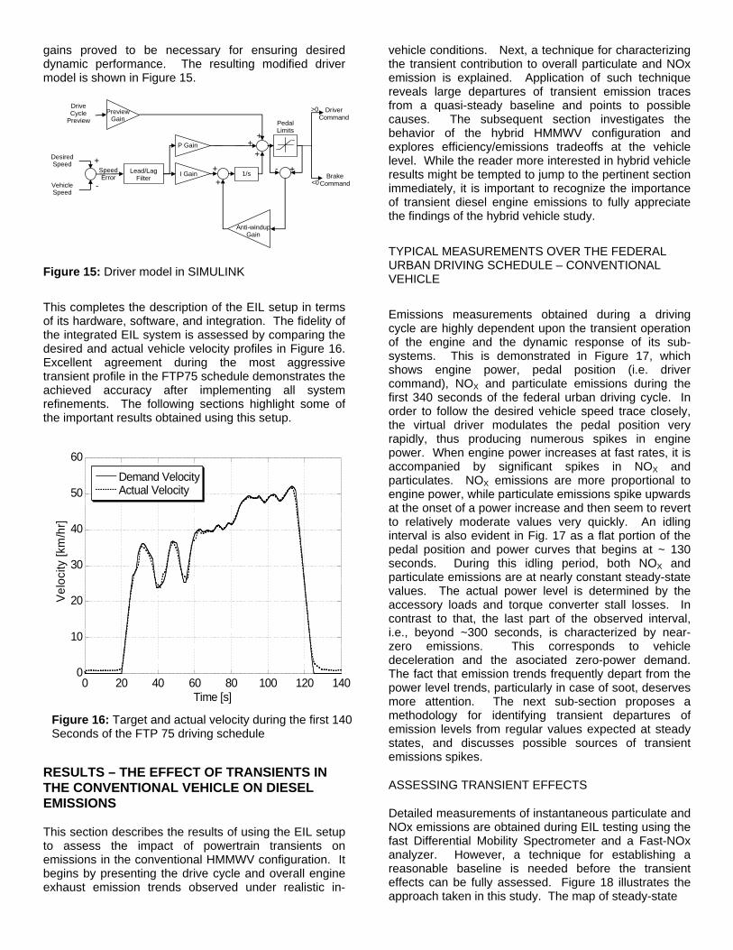
This completes the description of the EIL setup in terms of its hardware, software, and integration. The fidelity of the integrated EIL system is assessed by comparing the desired and actual vehicle velocity profiles in Figure 16. Excellent agreement during the most aggressive transient profile in the FTP75 schedule demonstrates the achieved accuracy after implementing all system refinements. The following sections highlight some of the important results obtained using this setup.

RESULTS – THE EFFECT OF TRANSIENTS IN THE CONVENTIONAL VEHICLE ON DIESEL EMISSIONS

This section describes the results of using the EIL setup to assess the impact of powertrain transients on emissions in the conventional HMMWV configuration. It begins by presenting the drive cycle and overall engine exhaust emission trends observed under realistic in-

vehicle conditions. Next, a technique for characterizing the transient contribution to overall particulate and NOx emission is explained. Application of such technique reveals large departures of transient emission traces from a quasi-steady baseline and points to possible causes. The subsequent section investigates the behavior of the hybrid HMMWV configuration and explores efficiency/emissions tradeoffs at the vehicle level. While the reader more interested in hybrid vehicle results might be tempted to jump to the pertinent section immediately, it is important to recognize the importance of transient diesel engine emissions to fully appreciate the findings of the hybrid vehicle study.

TYPICAL MEASUREMENTS OVER THE FEDERAL URBAN DRIVING SCHEDULE – CONVENTIONAL VEHICLE

Emissions measurements obtained during a driving cycle are highly dependent upon the transient operation of the engine and the dynamic response of its sub-systems. This is demonstrated in Figure 17, which shows engine power, pedal position (i.e. driver command), NOX and particulate emissions during the first 340 seconds of the federal urban driving cycle. In order to follow the desired vehicle speed trace closely, the virtual driver modulates the pedal position very rapidly, thus producing numerous spikes in engine power. When engine power increases at fast rates, it is accompanied by significant spikes in NOX and particulates. NOX emissions are more proportional to engine power, while particulate emissions spike upwards at the onset of a power increase and then seem to revert to relatively moderate values very quickly. An idling interval is also evident in Fig. 17 as a flat portion of the pedal position and power curves that begins at ~ 130 seconds. During this idling period, both NOX and particulate emissions are at nearly constant steady-state values. The actual power level is determined by the accessory loads and torque converter stall losses. In contrast to that, the last part of the observed interval, i.e., beyond ~300 seconds, is characterized by near-zero emissions. This corresponds to vehicle deceleration and the asociated zero-power demand. The fact that emission trends frequently depart from the power level trends, particularly in case of soot, deserves more attention. The next sub-section proposes a methodology for identifying transient departures of emission levels from regular values expected at steady states, and discusses possible sources of transient emissions spikes.

ASSESSING TRANSIENT EFFECTS

Detailed measurements of instantaneous particulate and NOx emissions are obtained during EIL testing using the fast Differential Mobility Spectrometer and a Fast-NOx analyzer. However, a technique for establishing a reasonable baseline is needed before the transient effects can be fully assessed. Figure 18 illustrates the approach taken in this study. The map of steady-state

Demand VelocityActual Velocity

0 20 40 60 80 100 120 1400

10

20

30

40

50

60

Time [s]

Velo

city

[km

/hr]

Figure 16: Target and actual velocity during the first 140 Seconds of the FTP 75 driving schedule

0

50

100

150

200

250

-150

-100

-50

0

50

100En

gine

Pow

er [k

W]

Pedal Position [%]

a)

0.00

0.05

0.10

0.15

0.20

0.25

NO

x [g

/s]

b)

0 85 170 255 3400.000

0.004

0.008

0.012

0.016

Time [s]

Parti

cula

te [g

/s]

c)

Figure 17: Histories of: a) pedal position, b) engine power, NOX, and particulate emissions, during first 340 Seconds of FTP 75 schedule emissions for a complete range of engine speeds and loads is measured first. The map is then inserted in the SIMULINK engine-in-vehicle simulation, such that it can provide NOx or PM concentration for any speed/fueling combination. Consequently, if speed and fueling histories measured in the EIL facility are provided to the engine module as input, the emission histories corresponding to assumed quasi-steady conditions are obtained as output. In other words, the quasi-steady baseline provides estimates of what the emissions would be had we marched through the driving schedule point-

by-point and allowed conditions to settle at every step. The real instantaneous measurements obtained on the EIL setup are then contrasted to this baseline in Fig. 19.

In particular, Figs. 19a and 19b show the instantaneous and quasi-steady mass flow rates of particulate and NOx, respectively, during the first half of the most aggressive vehicle speed profile in the FTP 75 cycle. The instantaneous particulate emission trace shows significantly higher spikes that precede the quasi-steady predictions. The instantaneous NOx trace demonstrates higher upward gradients and higher peaks, as well as sharp fluctuations during the 165s – 175s and 190-200s intervals.

In order to interpret these transient trends and understand possible causes for significantly higher peak emissions than what would be expected based on quasi-steady estimates, selected engine variables are plotted for the same time interval in Figure 20. The pedal position shows driver behavior and in the case of the conventional vehicle corresponds directly to the engine torque command, and the intake manifold pressure illustrates turbocharger response to the commanded load changes (see Fig. 20a). While the command often

pi/30

rpm_to_rad/s

1e-6

mg_to_kg

w (rad/s)

T (Nm)

mdot_fuel (mg/cy cle)

f uel use (g/s)

EOemis (g/s)

fuel use and EO emis

Torque Look-UpTable (2-D)

Fuel.mat

To Fi le2

engine_speed.mat

To Fi le1

emis.mat

To File

Time

Engine Speed (rpm)

Fuel Flow (mg/Strk)

Driving Cycle

Clock

Steady-stateNOx Map

Steady-stateNOx Map

160 170 180 190 200 210 2200.00

0.03

0.06

0.09

0.12

0.15

Time [s]

NO

x [g

/s]

0 200 400 600 800 1000 1200 1400500

1000

1500

2000

2500

3000

Time [s]

Engi

ne S

peed

[rpm

] Engine speed

0 200 400 600 800 1000 1200 1400500

1000

1500

2000

2500

3000

Time [s]

Engi

ne S

peed

[rpm

] Engine speed

0 200 400 600 800 1000 1200 14000

3

6

9

12

Time [s]

Fuel

Flo

w [g

/s] Fueling rate

0 200 400 600 800 1000 1200 14000

3

6

9

12

Time [s]

Fuel

Flo

w [g

/s] Fueling rate

Figure 18: Methodology for obtaining the quasi-steady emissions baseline corresponding to conditions experienced during a driving schedule

shows very rapid increases to 100%, the intake manifold pressure buildup is delayed due to turbocharger inertia and manifold filling dynamics. Hence, there is a period of irregular conditions, where the engine air supply limits the amount of fuel that can be burned, mixing is poor and the A/F ratio can be significantly higher than under more steady operation. In addition, there may be some exhaust residual still lingering in the manifold even if the EGR valve is instantly closed. These transient departures have the most effect on particulate emissions at the very initiation of the step increase in load, hence the advanced phasing of instantaneous PM spikes. They cause a tangible increase of integrated area under the curve during the transient interval. In contrast, the quasi steady profile basically follows the load, hence its peak is aligned with the peak in boost pressure.

The intensity of transient variations of engine operating conditions can be judged from the rates of change of engine speed and power, given in Fig. 20b. The profile of the rate of power variations correlates qualitatively with the instantaneous NOx trends. Peaks of dPower/dt align well with transient NOx spikes. Correlation with the engine acceleration is weaker (see the 165 second interval), hence the increase in fueling/torque is more dominant. In addition, peak NOx emissions have a second order dependence on the power level at the initiation of the transient. As an example, the peak dPower/dt values at ~187 seconds is higher than at ~193 seconds, but the NOx spike corresponding to the latter is much greater. The former transient follows a period of idling, while the subsequent one begins at a much higher initial load level thus yielding more NOx. In

Quasi-SteadyTransient Measurement

160 170 180 190 200 210 2200.000

0.003

0.006

0.010

0.013

0.016

Time [s]

Parti

cula

te [g

/s]

Quasi-SteadyTransient Measurement

160 170 180 190 200 210 2200.00

0.05

0.10

0.15

0.20

0.25

Time [s]

NO

x [g

/s]

a) b) Figure 19: Comparison of measured transient emissions and predictions based on quasi-steady assumptions and steady-state measurements, during a 160 – 220 sec. interval of the FTP 75: a) particulates, and b) NOx

0

25

50

75

100

125

100

130

160

190

220

250

160 170 180 190 200 210 220

Ped

al P

ositi

on [%

]

Intake Manifold P

ressure [kPa]

Time [s]

-200

-100

0

100

200

300

400

500

600

-3000

-2500

-2000

-1500

-1000

-500

0

500

1000

160 170 180 190 200 210 220

dPow

er/d

t

dSpeed/dt

Time [s] a) b) Figure 20: Variables characterizing engine system behavior during a 160 – 220 sec. interval of the FTP 75: a) pedal position and measured intake manifold pressure, and b) rates of change of engine speed and power.

summary, quantitative analysis suggests a very high magnitude of transient effects on emissions, and obvious shortcomings of any approaches based on steady-state measurements.

RESULTS – THE EFFECT OF HYBRID POWER MANAGEMENT ON FUEL ECONOMY AND EMISSIONS

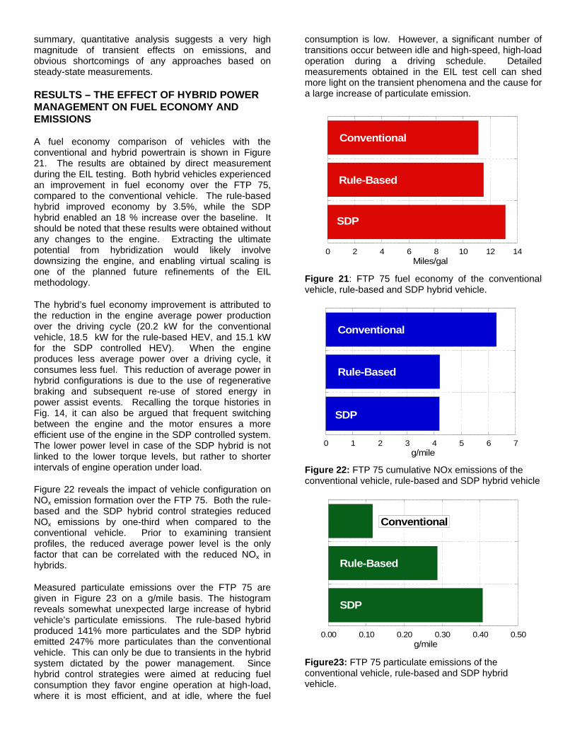
A fuel economy comparison of vehicles with the conventional and hybrid powertrain is shown in Figure 21. The results are obtained by direct measurement during the EIL testing. Both hybrid vehicles experienced an improvement in fuel economy over the FTP 75, compared to the conventional vehicle. The rule-based hybrid improved economy by 3.5%, while the SDP hybrid enabled an 18 % increase over the baseline. It should be noted that these results were obtained without any changes to the engine. Extracting the ultimate potential from hybridization would likely involve downsizing the engine, and enabling virtual scaling is one of the planned future refinements of the EIL methodology.

The hybrid’s fuel economy improvement is attributed to the reduction in the engine average power production over the driving cycle (20.2 kW for the conventional vehicle, 18.5 kW for the rule-based HEV, and 15.1 kW for the SDP controlled HEV). When the engine produces less average power over a driving cycle, it consumes less fuel. This reduction of average power in hybrid configurations is due to the use of regenerative braking and subsequent re-use of stored energy in power assist events. Recalling the torque histories in Fig. 14, it can also be argued that frequent switching between the engine and the motor ensures a more efficient use of the engine in the SDP controlled system. The lower power level in case of the SDP hybrid is not linked to the lower torque levels, but rather to shorter intervals of engine operation under load.

Figure 22 reveals the impact of vehicle configuration on NOx emission formation over the FTP 75. Both the rule-based and the SDP hybrid control strategies reduced NOx emissions by one-third when compared to the conventional vehicle. Prior to examining transient profiles, the reduced average power level is the only factor that can be correlated with the reduced NOx in hybrids.

Measured particulate emissions over the FTP 75 are given in Figure 23 on a g/mile basis. The histogram reveals somewhat unexpected large increase of hybrid vehicle’s particulate emissions. The rule-based hybrid produced 141% more particulates and the SDP hybrid emitted 247% more particulates than the conventional vehicle. This can only be due to transients in the hybrid system dictated by the power management. Since hybrid control strategies were aimed at reducing fuel consumption they favor engine operation at high-load, where it is most efficient, and at idle, where the fuel

consumption is low. However, a significant number of transitions occur between idle and high-speed, high-load operation during a driving schedule. Detailed measurements obtained in the EIL test cell can shed more light on the transient phenomena and the cause for a large increase of particulate emission.

0 2 4 6 8 10 12 14Miles/gal

Rule-Based

Conventional

SDP

Figure 21: FTP 75 fuel economy of the conventional vehicle, rule-based and SDP hybrid vehicle.

0 1 2 3 4 5 6 7g/mile

Conventional

SDP

Rule-Based

Figure 22: FTP 75 cumulative NOx emissions of the conventional vehicle, rule-based and SDP hybrid vehicle

0.00 0.10 0.20 0.30 0.40 0.50g/mile

Conventional

Rule-Based

SDP

Figure23: FTP 75 particulate emissions of the conventional vehicle, rule-based and SDP hybrid vehicle.

The transient behavior of the engine system in the conventional and hybrid SDP powertrain is examined in Figures 24 and 25. Engine command and particulate emission traces during the relatively aggressive interval in the city driving schedule are compared in Figures 24a and 24b. The driver sends aggressive signals to the engine in the conventional powertrain only at the initiation of hard acceleration at the beginning of the interval (see Fig 24a). A large spike in soot emission is visible in the first ten-second segment, while the rest of

the trace follows the commanded load relatively closely. In contrast, the SDP algorithm initiates frequent switching between zero-demand and near-100% demand. While engine operation at high load increases efficiency, it comes with a price, i.e. every step increase in engine command is accompanied by a spike in particulate emissions. This clearly illustrates a tradeoff between fuel economy and soot emission at the vehicle level, when power management is aggressively

0

0.01

0.02

0.03

0.04

0.05

-150

-100

-50

0

50

100

185 205 225 245 265 285 305

Engine Com

mand [%

]

Conventional Vehicle

Parti

cula

te E

mis

sion

s [g

/s]

Time [s]

Engine Command

PM

a)

0

0.01

0.02

0.03

0.04

0.05

-150

-100

-50

0

50

100

185 205 225 245 265 285 305

Parti

cula

te E

mis

sion

s [g

/s]

Engine Com

mand [%

]

Time [s]

EngineCommand

SDP Hybrid

PM

b)

Figure 24: Comparison of transient engine torque command and measured particulate emission signals in the: a) conventional and b) hybrid propulsion system with SDP power management.

0

0.1

0.2

0.3

0.4

0.5

0.6

-1500

-750

0

750

1500

2250

3000

185 215 245 275 305

NO

x Em

issi

ons

[g/s

]

Engine Speed [rpm

]

Time [s]

Conventional Vehicle

NOx

Engine Speed

a)

0

0.1

0.2

0.3

0.4

0.5

0.6

-1500

-750

0

750

1500

2250

3000

185 215 245 275 305

NO

x Em

issi

ons

[g/s

]

Engine Speed [rpm

]

SDP Hybrid

Time [s]

Engine Speed

NOx

b)

Figure 25: Comparison of transient engine speed and measured NOx emission signals in the: a) conventional and b) hybrid propulsion system with SDP power management.

optimized for best efficiency. Coming off the high load intervals initiates frequent deceleration events in the hybrid system, as seen in Figure 25b. Deceleration events are accompanied with zero fueling, thus the

corresponding dips of NOx emissions seen in Fig. 25b. This reduces the area below the NOx curve and decreases the cumulative amount of nitric-oxides for the test.

In summary, the particulate emission profiles and extremely high peaks provide convincing evidence that power management of modern hybrids cannot be based only on fuel economy or steady-state emission considerations. An engine-in-the-loop technology allows insight into critical dynamic conditions as a necessary first step. Characterization of transients provides a basis for further work on devising engine-level (e.g. multiple injection) or vehicle-level (e.g. including emission constraints in optimal power management) strategies.

CONCLUSIONS

A real 6L V8 diesel engine was immersed in the virtual vehicle system to develop engine-in-the-loop capability. Two critical enablers were an advanced, highly-dynamic dynamometer setup and a suite of vehicle models with appropriate fidelity. The study emphasizes fundamental aspects of transient diesel emissions in the context of hybrid propulsion. Hence, the EIL setup included advanced engine instrumentation for monitoring key engine processes, as well as a fast NOx analyzer and a fast particle sizer (differential mobility spectrometer). This allowed detailed analysis of the effect of transient engine operating conditions on the instantaneous emission of pollutants. On the modeling side, a previously developed vehicle system modeling platform allowed reconfiguring of the vehicle architecture for evaluating different propulsion options for a medium off-road truck. In particular, a 4x4 conventional powertrain for the HMMWV was configured with a four-speed automatic transmission, while a hybrid option employed a parallel architecture with a post-transmission electric motor location. Two power management strategies were developed, based on a traditional rule-based approach and a stochastic dynamic programming technique, respectively. Proper modeling was used to enable real-time simulation, while preserving a required degree of fidelity.

The development of the EIL setup utilized a Matlab-SIMULINK interface provided by the vendor of the dynamometer and the accompanying control system. The implementation uncovered several integration challenges, such as the signal noise and stability issues, time delay in signal processing and inadequate cyber-driver response. These issues were addressed by reversing the causality of the torque converter model, the implementation of lead-lag filtering, and by introducing preview in the driver model.

The engine coupled to the virtual conventional and hybrid vehicle system was tested over the federal urban driving schedule. The analysis of results shows the following:

• Engine transients have very significant impact on instantaneous NOx and soot emission, with significant spikes occurring during initial phases of vehicle acceleration events.

• Transient particulate emissions show the largest departure from quasi-steady estimates at the

initiation of a sudden load increase, thus causing advanced phasing of instantaneous PM spikes. The conditions are characterized by turbo lag, i.e. low boost and poor mixing, and remnants of exhaust residual from preceding steady conditions.

• Transient NOx emissions correlate qualitatively with the rate of engine power variation. Peak values are significantly higher than quasi-steady estimates. In addition, there is a second-order dependence on the power level at the initiation of the transient.

• Hybridization of the HMMWV powertrain provides tangible improvements in fuel economy and NOx emissions, accompanied by a particulate emission penalty.

• The stochastic dynamic programming strategy enhances both the benefits and the penalty, with an 18% increase in fuel economy and more than doubling of particulate emission. This is attributed to the tendency of the algorithm to frequently switch between engine-only and motor-only operation. This places operating points of either component into a more efficient region, but every step increase in engine command is accompanied by a spike in particulate emissions. The reduction of NOx is attributed to frequent deceleration events accompanied with zero fueling. This more than offsets transient increases of instantaneous NOx emission during acceleration.

The observed tradeoff between the hybrid vehicle fuel economy and soot emission provides convincing evidence that power management of modern diesel hybrids cannot be based only on fuel economy and steady-state emission considerations. Rather, it requires characterization of transients as a basis for devising engine-level or vehicle level strategies. An example of the former would be multiple fuel injections or advanced intake-air handling, while the latter requires including emissions as constraints or part of the objective function in optimal power management approaches.

ACKNOWLEDGMENTS

The authors wish to acknowledge the technical and financial support of the Automotive Research Center (ARC) by the National Automotive Center (NAC), and the U.S. Army Tank-Automotive Research, Development and Engineering Center (TARDEC). The ARC is a U.S. Army Center of Excellence for Automotive Research at the University of Michigan, currently in partnership with the University of Alaska-Fairbanks, Clemson University, University of Iowa, Oakland University, University of Tennessee, and Wayne State University. Josef Mayrhofer of AVL is recognized for technical support with the experimental setup, and Burit Kittirungsi and Loucas Louca for their contribution to previous vehicle modeling efforts. The authors also wish to acknowledge the technical support of Greg Zhang from International Engine and Truck Corporation, and John Vanderslice and Kevin Gady from the Ford Motor Company.

REFERENCES

1. Lovins, A.B.,"Battling Fuel Waste in the Military", Rocky Mountain Institute Newsletter, Fall/Winter 2001 (http://www.rmi.org/sitepages/pid518.php).

2. Fluga, E. C., “Modeling of the Complete Vehicle Powertrain Using ENTERPRISE”, SAE Paper 931179, 1993.

3. Ciesla, C. R., Jennings, M. J., “A Modular Approach to Powertrain Modeling and Shift Quality Analysis”, SAE paper 950419, Special Publication SP-1080, 1995.

4. Rousseau, A., Sharer, P., Pasquier, M., “Validation process of a HEV system analysis model: PSAT“, SAE paper 2001-01-0953

5. Assanis, D., Filipi, Z., Gravante, S., Grohnke, D., Gui, X., Louca, L., Rideout, G., Stein, J., Wang, Y.,“Validation and Use of Simulink Integrated, High Fidelity, Engine-In-Vehicle Simulation of the International Class VI Truck,” SAE Technical Paper No. 2000-01-0288.

6. Lin, C-C., Filipi, Z., Loucas, L., Peng, H., Assanis, D., Stein, J.,”Modeling and Control for a Medium-Duty Hybrid Electric Truck”, International Journal of Heavy Vehicle Systems, Vol. 11, Nos. 3/4, 2004, pp. 349-370

7. Shidore, N., Pasquier, M., “Interdependence of System Control and Component Sizing for a Hydrogen-Fueled Hybrid Vehicle”, SAE paper 2005-01-3457

8. Kim, H. M., Kokkolaras, M., Louca, L.S., Delagrammatikas, G.J., Michelena, N.F., Filipi, Z.S., Papalambros, P.Y., Stein, J.L., Assanis, D.N., “Target Cascading in Vehicle Redesign: A Class VI Truck Study”, International Journal of Vehicle Design, Vol. 29, No. 3, Inderscience Enterprises, Geneva, 2002, pp. 199-225

9. Hong, S.-Ch., Rutland, C., Reitz, R., “Development of an Integrated Spray and Combustion Model for Diesel Simulations”, SAE paper 2001-30-0012, 2001.

10. Hong, S., Assanis, D., Wooldridge, M., “Multi-dimensional modeling of NO and soot emissions with detailed chemistry and mixing in a direct injection natural gas engine”, SAE paper 2002-01-1112, 2002.

11. Gomez, M., “Hardware-in-the-Loop Simulation”, http://www.embedded.com/story/OEG20011129S0054

12. Nabi, S., Balike, M., Allen, J., Rzemien, K., “An overview of hardware-in-the-loop testing systems at Visteon”, SAE paper 2004-01-1240, 2004.

13. Jason T. C., and Moskwa, J.J., “A Hardware-in-the-Loop Transient Diesel Engine Test System for Control and Diagnostic Development”, Proceedings of the ASME International Mechanical Engineering Congress and Exposition, New York, 2001

14. Fleming, M., Len, G., Stryker, P., “Design and Construction of a University-Based Hybrid Electric Powertrain Test Cell”, SAE Technical Paper 2000-01-3106.

15. “Diesel Hybridization and Emissions”, Argonne National Laboratory Center for Transportation Research, Report to DOE from the ANL Vehicle Systems and Fuels Team, available electronically at http://www.osti.gov/bridge/, in paper from U.S. Department of Energy, Office of Scientific and Technical Information, P.O. Box 62, Oak Ridge, TN 37831-0062.

16. Filipi, Z., Wang, Y., Assanis, D.,”Variable Geometry Turbine (VGT) Strategies for Improving Diesel Engine In-Vehicle Response - a Simulation Study”, International Journal of Heavy Vehicle Systems, Vol. 11, Nos. 3/4*, 2004, pp. 303-326.

17. Wijetunge, R. S., Brace, C. J., Hawley, J. G., Vaughan, N. D., Horrocks, R. W., and Bird, G. L., “Dynamic Behavior of a High Speed Direct Injection Diesel Engine,” SAE Transactions—Journal of Engines, Vol. 108, Paper No. 1999-01-0829, 1999.

18. Hofeldt, D., Chen, G.,“Transient particulate emissions from diesel buses during the central business district cycle”, SAE Technical Paper 960251.

19. Lin, C., Filipi, Z., Wang, Y., Louca, L., Peng, H., Assanis, D., Stein, J., “Integrated, Feed-forward Hybrid Electric Vehicle Simulation in SIMULINK and its Use for Power Management Studies,” SAE Technical Paper 2001-01-1334, 2001.

20. Lin, C-C., Filipi, Z., Loucas, L., Peng, H., Assanis, D., Stein, J.,”Modeling and Control for a Medium-Duty Hybrid Electric Truck”, International Journal of Heavy Vehicle Systems, Vol. 11, Nos. 3/4, 2004, pp. 349-370

21. Kokkolaras, M., Mourelatos, Z., Louca, L., Filipi, Z.S., Delagrammatikas, G., Stefanopoulou, A., Papalambros, P., Assanis, D.N.,“Design under Uncertainty and Assessment of Performance Reliability for a Dual-Use Medium Truck with Hydraulic-Hybrid Powertrain and Fuel Cell Auxiliary Power Unit”, SAE paper 2005-01-1396, SAE Transactions, Journal of Materials Manufacturing & Engineering, 2005.

22. Wu, B., Lin, C.-C., Filipi, Z., Peng H., Assanis, D., “Optimal Power Management for a Hydraulic Hybrid Delivery Truck”, Journal of Vehicle System Dynamics, Vol. 42, Nos. 1-2, 2004, pp. 23-40.

23. Filipi, Z., Loucas, L., Daran, B., Lin, C-C., Yildir, U., Wu, B., Kokkolaras, M., Assanis, D., Peng, H., Papalambros, P., Stein, J., Szkubiel, D., Chapp, R.,”Combined Optimization of Design and Power Management of the Hydraulic Hybrid Propulsion System for the 6x6 Medium Truck”, International Journal of Heavy Vehicle Systems, Vol. 11, Nos. 3/4, 2004, pp. 371-401

24. Knafl, A., Hagena, J.R., Filipi, Z.S., Assanis, D.N., “Dual-Use Engine Calibration: Leveraging Modern Technologies to Improve Performance - Emissions Tradeoff”, SAE paper 2005-01-1549

25. Partridge, W., Storey, J., Lewis, S., Smithwick, R., DeVault, G., Cunningham, M., Currier, N., and Yonushonis, T., “Time-Resolved Measurements of Emission Transients By Mass Spectrometry,” SAE Paper No. 2000-01-2952, SAE Transactions—Journal of Fuels and Lubricants, Vol. 109, 2000.

26. Reavell, K., Hands, T., and Collings, N., “A Fast-Response Particulate Spectrometer for Combustion Aerosols,” SAE Paper No. 2002-01-2714, SAE Transactions—Journal of Fuels and Lubricants, Vol. 111, 2002.

27. Park, K., Cao, F., Kittelson, D. B., and McMurry, P. H., “Relationship Between Particle Mass and Mobility for Diesel Exhaust Particles,” Environmental Science and Technology, Vol. 37, No. 3, pp. 577-583, 2003.

28. Kozaki, T., Mori, H., Fathy, H. K., Gopalswamy, S., “Balancing the Speed and Fidelity of Automotive Powertrain Models Through Surrogation”, Proceedings of the 2004 ASME International Mechanical Engineering Congress and Exposition, Anaheim, California, 2004.

29. Stein, J. L., and Wilson, B. H., “An Algorithm for Obtaining Proper Models of Distributed and Discrete Systems”, Transactions of the ASME: Journal of Dynamic Systems, Measurement, and Control, 117 (4), 1995, pp. 534-540.

30. Louca, L. S. and Yildir, U. B., “Modeling and Reduction Techniques for Studies of Integrated Hybrid Vehicle Systems”, Proceedings of the 4th International Symposium on Mathematical Modeling, Vienna, Austria, 2003

31. Louca, L., Stein, J., Rideout, D., “Generating Proper Integrated Dynamic Models for Vehicle Mobility Using a Bond Graph Formulation,” Society for Computer Simulation, Phoenix, AZ, January 2001.

32. Karnopp, D. C., Margolis, D. L., and Rosenberg, R. C., System Dynamics: Modeling and Simulation of Mechatronic Systems, 3rd ed., John Wiley & Sons, 2000.

33. Sendur, P., Stein, J. L., Louca, L. S., Peng, H., “A Model Accuracy and Validation Algorithm”, Proceedings of the 2002 ASME International

Mechanical Engineering Congress and Exposition, New Orleans, Louisiana, 2002.

34. Louca, L. S., and J. L. Stein, J. L.,“Energy-Based Model Reduction of Linear Systems”, Proceedings of the International Conference on Bond Graph Modeling and Simulation, San Francisco, California, 1999.

35. Fathy H. K., Stein, J. L., “Fundamental Concordances between Balanced Truncation and the Model Order Reduction Algorithm”, Proceedings of the 2nd International Conference on Integrated Modeling and Analysis in Applied Control and Simulation, Marseilles, France, 2005.

36. Fathy, H. K., Ahlawat, R., Stein, J. L., “Proper Powertrain Modeling for Engine-in-the-Loop Simulation”, Proceedings of the 2005 ASME International Mechanical Engineering Congress and Exposition, Orlando, Florida, 2005.

37. 20SIM, 20SIM Pro User’s Manual. The University of Twent-Controllab Products B.V. Enschede, The Netherlands, 1999.

38. Johnson, V., Wipke, K., Rausen, D., “HEV Control Strategy for Real-Time Optimization of Fuel Economy and Emissions”, SAE Technical Paper No. 2000-01-1543, 2000.

39. Lin, C., Peng H., Grizzle, J., “A Stochastic Control Strategy for Hybrid Electric Vehicles,” Proceedings of the 2004 American Control Conference, Boston, MA, 06/30-07/02, 2004.

40. Peng, H., Kim, M., Lin, C., Grizzle, J., “Integrated Dynamic Simulation Model with Supervisory Control Strategy for a PEM Fuel Cell Hybrid Vehicle,” Proceedings of ASME International Mechanical Engineering Congress and Exposition, November 13-19, 2004, Anaheim, California USA, IMECE2004-61775.

41. Bertsekas, D. P., Dynamic Programming and Optimal Control. Athena Scientific, 1995.

42. Babbit, G. R., and Moskwa, J. J.,“Implementation Details and Test Results for a Transient Engine Dynamometer and Hardware in the Loop Vehicle Model”, Proceedings of the IEEE International Symposium on Computer-Aided Control System Design, Hawaii, 1999.

43. Hrovat, D., Tobler, W.F., “Bond Graph Modeling and Computer Simulation of Automotive Torque Converters”, Journal of the Franklin Institute, 319 (12), pp. 93-114, 1985.

44. Franklin, G. F., Powell, J. D., and Emami-Naeini, A., Feedback Control of Dynamic Systems, 3rd ed. Addison-Wesley, 1994.

45. Skogestad, S., and Postlethwaite, I., Multivariable Feedback Control: Analysis and Design, John Wiley & Sons, 1997.