energy research and development division final project …energy research and development division...

Energy Research and Development Division

FINAL PROJECT REPORT

Effect of Variable Fuel Composition on Emissions and Lean Blowoff Stability Performance Analysis of Nine Industrial Combustion Applications

Appendix B - Burner Configuration #2: Surface Stabilized Combustion

California Energy Commission Edmund G. Brown Jr., Governor

June 2017 | CEC-500-2017-026-APB

UCI Combustion Laboratory Burner Config. #2. Surface Stabilized Combustion

Burner Configuration # 2: Surface Stabilized Combustion

Emissions and Stability Performance

CEC Agreement No. 500-13-004

Prepared by:

Andrés Colorado and Vincent McDonell1

REV DESCRIPTION DATE APPROVED BY - Initial Release [06/05/2015] 1 Updated Appendix formatting [07/15/2015] 2 References [2/5/2016]

1 949 824 5950 x 11121; [email protected]


i | P a g e

Contents

EXECUTIVE SUMMARY .......................................................................................................................................................... v

Key Features .............................................................................................................................................................................. 1

Virtual AeroThermal Field - Computational Fluid Dynamics ................................................................................ 3

1.1. Domain and Mesh ................................................................................................................................................. 4

1.2. Boundary conditions........................................................................................................................................... 5

Chemical Reactor Network .................................................................................................................................................. 6

1.3. Zonal distribution ................................................................................................................................................ 6

1.4. Reactor Network Variables .............................................................................................................................. 7

1.5. Effect of Fuel Composition on Emissions ................................................................................................... 8

1.5.1. Fuel class I - Hydrogen enriched natural gas .................................................................................. 9

1.5.2. Fuel class II- Landfill / digester biogas ............................................................................................ 14

1.5.3. Fuel class III-Mixtures with heavier hydrocarbons .................................................................... 18

1.6. Stability analysis ................................................................................................................................................. 21

Appendix A: Interchangeability analysis .................................................................................................................. A-1

1.6.1. Interchangeability under the criterion of Flashback (AGA) ................................................. A-2

1.6.2. Interchangeability under the criterion of Lifting (AGA) ......................................................... A-3

1.6.3. Interchangeability under the criterion of yellow tipping (AGA)......................................... A-4

Appendix B: NOx pathways ............................................................................................................................................ B-1

Appendix C: Radiation calculations ............................................................................................................................ C-1

References .................................................................................................................................................................................. 1


ii | P a g e

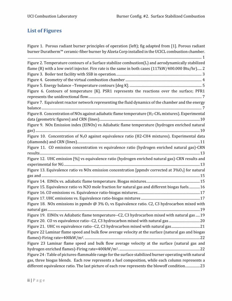
List of Figures

Figure 1. Porous radiant burner principles of operation (left); fig adapted from [1]. Porous radiant

burner Duratherm™ ceramic-fiber burner by Alzeta Corp installed in the UCICL combustion chamber.

......................................................................................................................................................................................................... 1

Figure 2. Temperature contours of a Surface stabilize combustion(L) and aerodynamically stabilized

flame (R) with a low swirl injector. Fire rate is the same in both cases (117kW/400.000 Btu/hr). .... 2

Figure 3. Boiler test facility with SSB in operation. .................................................................................................. 3

Figure 4. Geometry of the virtual combustion chamber ........................................................................................ 4

Figure 5. Energy balance –Temperature contours [deg K]. ................................................................................... 5

Figure 6. Contours of temperature [K]. PSR1 represents the reactions over the surface; PFR1

represents the unidirectional flow. .................................................................................................................................. 7

Figure 7. Equivalent reactor network representing the fluid dynamics of the chamber and the energy

balance ......................................................................................................................................................................................... 7

Figure 8. Concentration of NOx against adiabatic flame temperature (H2-CH4 mixtures). Experimental

data (geometric figures) and CRN (lines). ................................................................................................................... 10

Figure 9. NOx Emission index (EINOx) vs Adiabatic flame temperature (hydrogen enriched natural

gas) .............................................................................................................................................................................................. 10

Figure 10. Concentration of N2O against equivalence ratio (H2-CH4 mixtures). Experimental data

(diamonds) and CRN (lines).............................................................................................................................................. 11

Figure 11. CO emission concentration vs equivalence ratio (hydrogen enriched natural gas)-CRN

results ......................................................................................................................................................................................... 13

Figure 12. UHC emission [%] vs equivalence ratio (hydrogen enriched natural gas)-CRN results and

experimental for NG ............................................................................................................................................................. 13

Figure 13. Equivalence ratio vs NOx emission concentration [ppmdv corrected at 3%O2] for natural

gas and ....................................................................................................................................................................................... 15

Figure 14. EINOx vs. adiabatic flame temperature. Biogas mixtures. ............................................................. 15

Figure 15. Equivalence ratio vs N2O mole fraction for natural gas and different biogas fuels. ............ 16

Figure 16. CO emissions vs. Equivalence ratio-biogas mixtures ........................................................................ 17

Figure 17. UHC emissions vs. Equivalence ratio-biogas mixtures .................................................................... 17

Figure 18. NOx emissions in ppmdv @ 3% O2 vs Equivalence ratio. C2, C3 hydrocarbon mixed with

natural gas ................................................................................................................................................................................ 19

Figure 19. EINOx vs Adiabatic flame temperature--C2, C3 hydrocarbon mixed with natural gas ..... 19

Figure 20. CO vs equivalence ratio--C2, C3 hydrocarbon mixed with natural gas .................................... 20

Figure 21. UHC vs equivalence ratio--C2, C3 hydrocarbon mixed with natural gas ................................. 21

Figure 22 Laminar flame speed and bulk flow average velocity at the surface (natural gas and biogas

flames)-Firing rate=400kW/m2. ..................................................................................................................................... 22

Figure 23 Laminar flame speed and bulk flow average velocity at the surface (natural gas and

hydrogen enriched flames)-Firing rate=400kW/m2. ............................................................................................. 22

Figure 24 : Table of pictures-flammable range for the surface stabilized burner operating with natural

gas, three biogas blends. Each row represents a fuel composition, while each column represents a

different equivalence ratio. The last picture of each row represents the blowoff condition. ................ 23


iii | P a g e

Figure 25. Table of pictures-flammable range for the surface stabilized burner operating with natural

gas and hydrogen enriched natural gas. ...................................................................................................................... 24

Figure A-1. AGA Flashback index. ................................................................................................................................. A-2

Figure A-27. AGA Lifting index. ..................................................................................................................................... A-3

Figure A-28. AGA Yellow tipping index. Analysis of interchangeability for mixtures CH4-H2 and CO-H2

..................................................................................................................................................................................................... A-4


iv | P a g e

List of Tables

Table 1. Summary of emissions and stability/1 .......................................................................................................... v

Table 2. Summary of emissions for interchangeable mixtures (AGA)/3 ......................................................... vi

Table 3. Equipment specification ..................................................................................................................................... 3

Table 4. CFD models .............................................................................................................................................................. 5

Table 5. Input variables used in the PSRs of the CRN model ................................................................................ 8

Table 6. Input variables used in the PFRs of the CRN model ............................................................................... 8

Table 7. Hydrogen enriched natural gas –Test fuels ................................................................................................ 9

Table 8. Biogas –Test fuels/1 ............................................................................................................................................ 14

Table 9. Mixtures with heavier hydrocarbons - Test fuels .................................................................................. 18

Table 10. Lean blow out limits. ...................................................................................................................................... 25

Table A-1. Summary of emissions for interchangeable mixtures (AGA) ..................................................... A-5


v | P a g e

Burner Configuration # 2: Surface Stabilized Combustion

EXECUTIVE SUMMARY A summary of the emissions and stability results for Burner Configuration #2, Surface StabilIzed

Combustion (SSC), is presented in Table 1. The table is coded with colors and trend indicators to

provide a simple overview of how fuel composition impacts the performance of Burner Configuration

#1.

Table 1. Summary of emissions and stability/1

Fuel class/2

I II III

Hydrogen

enriched

natural gas

(CH4+H2)

Biogas

(CH4+CO2)

Mixtures with

heavier

hydrocarbons

(C1/C2/C3)

NOx ↓ @↑H2 ↓@↑CO2 ↑@↑C2,C3..

CO ↓ @↑H2 ↑@↓CO2 ↑@↑C2,C3..

Stability ↑ @↑H2 ↓@↑CO2 ↑@↑C2,C3..

/1 Cells highlighted with red represent negative impacts on emissions or stability. Conversely, cells

highlighted with green represent positive effects.

/2 Fuel Class I: Hydrogen Containing Fuels

Fuel Class II: Diluted Fuels

Fuel Class III: Fuels with Higher Hydrocarbons


vi | P a g e

The example below illustrates how the table can be read:

Emissions Hydrogen enriched natural gas (CH4+H2)

Reading

NOx ↓ @↑H2 NOx decreases (↑) when adding (@) (↑) H2

CO ↓ @↑H2 CO decreases (↓) when adding (↑) H2

The following mixtures are interchangeable with natural gas according to the Wobbe Index and the

interchangeability indices for flashback, lifting and yellow tipping established by the American Gas

Association (AGA). Table 2 presents a summary indicating the expected increase (↑) or reduction (↓)

of NOx and CO concentration at a fixed 3% O2 concentration in the exhaust. The percent change

indicated in the table represents the change compared to the results for natural gas (Assumed as

100% CH4).

Table 2. Summary of emissions for interchangeable mixtures (AGA)/3

Fuel Mixture

Equivalence

Ratio NOx [ppmdv] CO [ppmdv]

at 3% O2

76% CH4 - 24% H2 0.87 ↓ 250% ↓ 40%

94% CH4 - 6% C2H6 0.87 ↑ 3% ↑ 6%

95% CH4 - 5% C3H8 0.87 ↑ 4% ↑ 3%

98% CH4 - 2% CO2 0.87 ↓ 3% ↑ 3%

/3 % change compared to 100% methane


1 | P a g e

Key Features The burner studied in this report is the Duratherm™ ceramic-fiber burner by Alzeta Corporation. The

porous radiant burner operation is summarized in Fig. 1. Premixed fuel and air flows through the

porous fiber material. The mixture heats as it passes through the material, and combustion takes

place on the outer surface. The combustion process continues in the gas phase as the flow leaves the

hot face of the material so that peak gas temperatures occur slightly beyond the hot face. Heat

transfer and diffusion of combustion products from the gas phase region back to the burner provide

the feedback necessary to sustain stable combustion. The flow of fuel-air mixture through the fiber

mat recuperates any inward conduction of heat from the outer surface such that the cold face of the

mat is very near the incoming gas mixture temperature. When the burner flame is fully attached to

the surface, the combustion occurs without any visible flame and without noise or pressure

fluctuations [1].

Figure 1. Porous radiant burner principles of operation (left); fig adapted from [1]. Porous radiant burner Duratherm™ ceramic-fiber burner by Alzeta Corp installed in the UCICL combustion chamber.

One distinctive characteristic of the surface stabilized combustion is the extended volume of the

reaction.

Figure 2 depicts this characteristic by comparing the volume of the surface stabilized reactions with

a dynamically stabilized flame (DSF). See BurnerReport # 1 (Low Swirl Injector) for more details [2].

At an equivalent firing rate of 117kW the ratio of flame volumes (SSC/LSB) is ~50 times. This

characteristic gives the surface stabilized burner an edge regarding direct radiation heat from the

flame to the load, as flame radiation is proportional to flame volume [3], in this case, the extended

surface cools down the reactions and favors ultra-low NOx emissions. Also the surface material re-

radiates part of the heat also cooling down the reactions.


2 | P a g e

Figure 2. Temperature contours of a Surface stabilize combustion(L) and aerodynamically stabilized flame (R) with a low swirl injector. Fire rate is the same in both cases (117kW/400.000 Btu/hr).

For this burner configuration, detailed data are made available from a test facility located in the UCI

Combustion Laboratory. Work is being carried out under CEC Contract 500-13-004 that is providing

data for the current effort.

The combustion chamber has 8 flat sides and is 2 feet in width and 3 feet in height (excluding exhaust

stack length). A picture of the furnace can be seen in Figure 3. The figure also presents the location

where the flame rests. Inside the furnace the walls near the optical windows are insulated with high

temperature insulation lining. The base around the burner is an extra-high temperature calcium

silicate insulation that comes in ½” thick 12”x12” sheets. This insulated layer limits the heat loss

from the burner to the aluminum plate supporting the entire furnace. There are three main parts to

the furnace: optical windows, water cooling panels, and exhaust stack. The water cooled panels are

located above the optical windows. Water enters from the bottom tubes and exits through the top

ring of tubing. During the tests the hot water in the boiler loop maintains a temperature of

approximately 100 degrees Fahrenheit. The purpose of the water cooling system is to minimize

structural damage to the furnace and simulate the thermal load of a commercial boiler. A summary

of the equipment specifications is presented in the following table.


3 | P a g e

Figure 3. Boiler test facility with SSB in operation.

Table 3. Equipment specification

Units

Maximum fire rate kW (Btu/hr) 117 (400,000)

Flame type Turbulent premixed - atmospheric

Equivalence ratio (ø) --- 0.45– 1 (NG)

Air preheating No

Application Boiler

Fuel(s) NG, biogas (up to 65% CO2 by vol.), hydrogen enriched NG (up to 30% H2 by vol.) C1 to C3 mixtures

Virtual AeroThermal Field - Computational Fluid Dynamics This section presents the details about the CFD simulation and the results that are used to build the

chemical reactor network. Total emissions are a primary function of temperature, oxygen

concentration, and the time the species spend under those conditions. The temperature profile, flow

field and concentration of species are presented and analyzed in this section. The methodology to

build a CRN consists on using the results of CFD simulations to divide the combustor volume into

zones represented by idealized reactor elements. Zones of the combustor where the gases flow in


4 | P a g e

one direction are modeled using PFRs; highly turbulent zones or zones with strong mixing are

modeled with PSRs. At the end of the section an equivalent CRN representing similar but simplified

fluid dynamics of the chamber is presented. The CRN is also similar regarding the volume the

reactors occupy in the combustion chamber, and the energy balance of the system.

1.1. Domain and Mesh A virtual chamber is used to model the fluid dynamics, heat transfer and heat release from the

reaction. In this case, the details regarding stability and emissions are not sought—only a relatively

time efficient calculation that can be used to guide the sectioning of the chamber into individual

reactors. Under the assumption of a cylindrical chamber (the actual chamber is octagonal) the

furnace is simulated with a 2D axisymmetric model. Steady state, Reynolds-Averaged-Navier-Stokes

(RANS) simulations are conducted using the Software ANSYS Fluent, version 15.0. A non-structured,

quadrilateral mesh is used. The mesh consists of 18000 cells, with a maximum aspect ratio of 2.7 and

minimum orthogonal quality of 0.58 The geometry and names of the boundary conditions are

presented in Figure 4. A summary of the models is presented in Table 4.

Figure 4. Geometry of the virtual combustion chamber


5 | P a g e

Table 4. CFD models

Mesh 2 D – non structured – 18000 cells Solver Steady

Pressure based Axisymmetric

Viscous model K-ε standard with enhanced wall functions Radiation P1 Species model Partially Premixed combustion - turbulent flame speed model -

Zimmont Density Incompressible ideal gas model pressure velocity coupling

SIMPLE: relationship between velocity and pressure corrections to enforce mass conservation and to obtain the pressure field

1.2. Boundary conditions The boundary conditions are set to match the energy balance of the actual system. This approach is

useful to describe more precisely the energy flow through the chamber, which leads to a more

accurate result for temperature field in the combustion chamber. The distribution of energy flow

through the combustor is fairly constant regardless the fuel type, around ~50% heat losses

correspond to the sensible heat loss with the exhaust gases, ~25% heat loss through the water cooled

walls and ~25% through the rest of the walls including the floor. Using the previous energy balance,

an approximate temperature field is predicted. The results for temperature distribution are

presented in Figure 5.

Figure 5. Energy balance –Temperature contours [deg K].

Also, for modeling the gas injection through the surface a mass flow inlet boundary type is used.


6 | P a g e

Chemical Reactor Network The chemical reactor modeling is found to be a valuable tool in the evaluation of pollutant formation

and the blow-out performance of combustion systems. The methodologies of the development vary

between authors [4]. In this study, the chemical reactor network is constructed based on the

computational fluid dynamics (CFD) results presented above. The concept of modeling a combustor

using chemical reactors such as perfectly stirred reactors (PSR), plug flow reactors (PFR) was first

introduced by S. L. Bragg [5]. A reactor network is defined to model the pollutant formation with a

detailed chemistry. On the other hand the introduction of a complex reaction mechanism in 3D

turbulent combustion codes is still too CPU time intensive to be applied in an industrial context. CFD

solvers could not be efficiently used to solve chemical equations due to the stiffness of the underlying

reaction scheme and the great number of species that it contains [6].

1.3. Zonal distribution In order to develop the CRN, the first step is divide the combustor volume into the distinct regions or

zones. Each of the zones is characterized by the particular physical properties of the flow and the

flame behavior. The two basic models used to build the network of reactors are the perfectly stirred

reactor (PSR) and the plug flow reactor (PFR).

• A PSR (i.e., a continuously stirred tank reactor) presumes that mixing to the molecular scale

occurs. Highly turbulent regions, premixed flows, and turbulent premixed reactions can be

modeled with this reactor. In this reactor, the chemical reaction occurs homogeneously.

• A PFR assumes that the flow moves as a “plug” and the chemical reaction proceeds one-

dimensionally, longitudinal mixing in the reactor is assumed to be zero. One limitation of this

model is that it can’t receive more than one stream. The composition at the entrance of the

reactor has to be defined.

As shown in Figure 6, the first zone corresponds to the volume of the premixed reaction and it is

represented by the PSR1. The zone downstream of PSR1 is considered the immediate post flame, the

temperatures in that region are the highest but also uniform. In the central zone of the flow field the

velocity vectors are unidirectional; therefore it is ideally represented with a PFR (PFR1). The post

flame region is important regarding the time the species spend in that zone. At that point the

combustion products are mainly carbon dioxide (CO2), water (H2O), remaining of oxygen (O2) and

nitrogen (N2); also a lower proportion of pollutant species like NOx and products of incomplete

combustion like carbon monoxide (CO) and unburned hydrocarbon appear in that region. The

reactions at that point are slow compared to the active flame region (PSR1). In particular the long

residence time in that region will help to oxidize the remaining CO into CO2, but also will help to

increase the NOx emissions if the temperature conditions are favorable for the nitrogen chemistry.


7 | P a g e

Figure 6. Contours of temperature [K]. PSR1 represents the reactions over the surface; PFR1 represents the unidirectional flow.

After connecting all the reactors, the reactor network is an equivalent and simplified representation

of the mixing process in the chamber and the energy balance of the system. Only the volumes of the

flame and near flame surroundings are necessary to model the reactions in the network. The reactor

network that represents the SSC is presented in Figure 7.

Figure 7. Equivalent reactor network representing the fluid dynamics of the chamber and the energy balance

1.4. Reactor Network Variables Each PSR in the network requires the following input variables:

Residence time (Rt), which is the average time the species spend in a particular system. This

variable can be related to the volume (𝑉) of the reactor, the average gas density (ρ) and the

mass flow (�̇�) through the following expression: 𝑅𝑡 =𝜌𝑉

�̇�


8 | P a g e

Mass flow through the reactor (�̇�)

Initial temperature

Pressure

Heat losses

The PFRs require the following input variables:

Length.

Diameter. This can be a function of the distance.

Initial temperature

Pressure

Heat losses

A summary of the variables used in the CRN model for Burner Configuration #2 are presented in

Table 5 and 6. Notice that the most important heat losses are related to the reactors close to the walls.

Also the residence time indicates that, not surprisingly, the gases spend relatively long periods of

time in the recirculation zones. In terms of connecting to design, species that are influenced by

residence time can be impacted by altering the size and temperature of these zones.

Table 5. Input variables used in the PSRs of the CRN model

Reactor name

Equivalence ratio

Vol (cm3) Firing rate (kW) Mass flow: air + fuel (kg/s)

Heat losses (%)

PSR_1 0.4 – 1 Fuel lean

Constant 10860

Constant 117 Variable depending on fuel composition and Equivalence ratio

Variable depending on fuel composition and ER. Approximation with (Radcal model for premixed flames) [3]

Table 6. Input variables used in the PFRs of the CRN model

Reactor name

Inlet radius (cm)

Length (cm) Heat losses (% of the total input)

PFR1 Constant 20

constant 1200

~25

1.5. Effect of Fuel Composition on Emissions In this section, the evaluation of the effect of the fuel composition on the emissions is assessed using

the CRN methodology. The power input to the burner is held constant at 117kW (400,000Btu/hr),

while the air flow rate is varied to control the flame temperature. This would mimic typical operation

of a boiler configuration in which the goal is to achieve certain temperature gain in the process.

A composition on a dry basis indicates that the water from the combustion products is removed

before the combustion products are analyzed with the gas analyzer. This presentation (ppmdv) is

representative of the measures in the field and is also typical of units found in regulatory or permit

limits. While this presentation is important and common, when comparing results among

significantly different fuel types, it can create some challenges in the interpretation of the results


9 | P a g e

comparing fuels. As a result, the results are also presented in form of an emission index (EI) which

represents a more absolute quantity. Volumetric fractions such as “ppm” indicate a relative

proportion of the pollutant in the pool of species. Emission index is the emission rate of a given

pollutant from a given source relative to the intensity of a specific activity or parameter. In this report,

emission indices are presented as mass of pollutant (in milligrams-mg) per unit of energy consumed

(kWh_fuel burned) (it is noteworthy that this index does not take into account the efficiency of the

system). The emissions index expressed as burnedfuel

pollutatnt

kWh

g

_

relates the total mass of pollutant emitted

per energy of fuel put into the system. When the emissions are plotted against equivalence ratio or

the adiabatic flame temperature, they represent the dependency of the emissions on the relative

proportion of available oxygen or the temperature of the reactions, respectively.

The CRN results for emissions and lean blow off limits were obtained using Chemkin Pro 15131 and

the GRI 3.0 reaction mechanism [7]. While it is recognized that the specific chemistry mechanism

used can influence the absolute values of the emissions predicted [8], the trends are generally

insensitive to the mechanism used.

1.5.1. Fuel class I - Hydrogen enriched natural gas

The fuel compositions of the CH4/H2 mixtures are presented in Table 7. The table also includes the

Wobbe index for each blend.

Table 7. Hydrogen enriched natural gas –Test fuels

Hydrogen enriched natural gas Wobbe index (BTU/scf)

10% CH4 – 90% H2 1095 30% CH4 – 70% H2 1095 50% CH4 – 50% H2 1144 70% CH4 – 30% H2 1205

Figure 8 and Figure 9 present the trends in form of NOx concentration and emission index,

respectively. As shown, predicted levels and some measured levels are shown for various fuel

compositions. . The CRN and experimental results for Nitrous oxides (N2O) are presented in Figure

10.


10 | P a g e

Figure 8. Concentration of NOx against adiabatic flame temperature (H2-CH4 mixtures). Experimental data (geometric figures) and CRN (lines).

Figure 9. NOx Emission index (EINOx) vs Adiabatic flame temperature (hydrogen enriched natural gas)

0

5

10

15

20

25

30

35

40

45

0.4 0.5 0.6 0.7 0.8 0.9 1

NO

x [p

pm

dv

@ 3

% O

2]

Equivalence ratio []

Natural gas experiment

30H2-70CH4 experiments

100 CH4 CRN

30H2-70CH4 CRN

50H2-50CH4 CRN

90H2-10CH4 CRN

0

0.01

0.02

0.03

0.04

0.05

0.06

1400 1600 1800 2000 2200 2400

EIN

Ox

[gN

Ox/

kWh

_fu

el b

urn

ed]

Adiabatic flame temerature []

Natural gas experiment

30H2-70CH4 experiments

100 CH4 CRN

30H2-70CH4 CRN

50H2-50H2 CRN

90H2-10CH4 CRN


11 | P a g e

Figure 10. Concentration of N2O against equivalence ratio (H2-CH4 mixtures). Experimental data (diamonds) and CRN (lines).

A summary of the key points regarding the behavior of NOx emissions for Fuel Class I include:

At a fixed equivalence ratio, the addition of hydrogen to natural gas reduces the production

of NOx.

The addition of H2 promotes the formation of intermediate species like OH and H, which

increase the burning velocity of the mixture. Given the higher burning velocity of the

hydrogen enriched fuels, it is expected that their reactions are more closely attached to the

surface. As a result the reactions transfer heat more efficiently to the surface while cooling

down the reactions more efficiently than a less attached flame, such as the biogas case.

The reactions flow in one direction and it is assumed that there is no gas recirculation effect.

At equivalence ratios above 0.85, NOx produced through the Zeldovich route or thermal

mechanism is dominant for all the fuels.

A consequence of the high reactivity of hydrogen is a reduced flame thickness also related to

an increase of the laminar flame speed. In this case high reactivity favors the heat transfer as

the reactions attach to the surface more efficiently with a highly reactive fuel.

For higher concentrations of hydrogen the heat losses from the PSR1 were increased from

the estimated values calculated with the RADCAL model. The RADCAL model is useful to

model the direct radiation of premixed flames. Without increasing the heat losses from the

PSR, the NOx trends show that the addition of hydrogen increases the emissions of NOx. Since

the experimental trends indicated a reduction of the NOx emissions, one logical explanation

is an increased heat transfer from the reactions compared to the natural gas case.

The percent increased of heat transfer from the PSR for the mixtures is as follows:

o 30H2/70CH4. Heat losses = 110% (as calculated with RADCAL)

o 50H2/50CH4. Heat losses = 120% (as calculated with RADCAL)

o 90H2/10H2. Heat losses=150% (as calculated with RADCAL)

0.0E+00

2.0E-07

4.0E-07

6.0E-07

8.0E-07

1.0E-06

1.2E-06

1.4E-06

0.30 0.40 0.50 0.60 0.70 0.80 0.90 1.00 1.10

N2O

mo

le f

ract

ion

[]


30 H2-70 CH4 experiment

30H2-70CH4 CRN

50H2-50CH4 CRN

90H2-10CH4 CRN

100 CH4 CRN


12 | P a g e

o The additional heat loss 10, 20 and 50% is attributed to the radiation from the surface

itself. This is, the flame radiates directly a portion equivalent to the 100% heat losses

estimated with RADCAL, while the surface radiates the additional portion heat.

For the fuel mixture with 90%H2-10% CH4 the NOx levels increased compared to the

50%H2/50%CH4 case. In this case the effect of the chemistry dominates the production of

NOx. The heat losses for this mixture point were assumed as 150% the calculated value.

Also the addition of H2 promotes the formation of intermediate species like OH and H, which

form more NOx through the NNH, thermal and N2O routes compared to pure hydrocarbon

flame. On the other hand, the prompt path is initiated by rapid reactions of hydrocarbon

radicals with molecular nitrogen; therefore the addition of H2 to the fuel reduces the

formation of NOx through the prompt route. Again the addition of H2 increases the burning

velocity and the heat transfer to the surface. The combined result is a reduced production of

NOx for the hydrogen enriched fuels, mainly attributed to the additional heat transfer to the

surface that acts as a heat sink cooling down the reactions.

Nitrous oxide (N2O) was measured during the experiments for natural gas and 70CH4/30H2.

See Figure 10 . For both cases fuel mixtures it was observed a maximum of ~ 1.2 ppmdv

(uncorrected) at an equivalence ratio of 0.45. This points of maximum N2O also coincided

with the lean blow out condition and the maximum emissions of CO and UHC. On the other

hand the CRN results show insignificant quantities of N2O compared to the experimental data.

At a fixed flame temperature, the addition of hydrogen to natural gas reduces the production

of NOx per energy consumed. At temperatures above 1900K, NOx produced through the

Zeldovich route or thermal mechanism is dominant for all the fuels.

Figure 9 indicates that is possible to reach higher flame temperatures with hydrogen

enriched fuels than with pure natural gas. At the same time with the addition of hydrogen

the emissions of NOx are reduced. The 90H2/10CH4 blend produces the lowest NOx levels at

the highest temperature. The combination of high temperature and low emissions is the goal

of any combustion designer, since higher temperatures maximize the efficiency of the

combustion system (increasing efficiency reduces the consumption of fuel and the carbon

footprint), and ultra-low or zero emissions represent the goal for environmentally friendly

applications.

The behavior of carbon monoxide (CO) and unburned hydrocarbons (UHC) is presented in Figure 11

and 11, respectively.


13 | P a g e

Figure 11. CO emission concentration vs equivalence ratio (hydrogen enriched natural gas)-CRN results

Figure 12. UHC emission [%] vs equivalence ratio (hydrogen enriched natural gas)-CRN results and experimental for NG

A summary of the key points regarding the behavior of CO and UHC emissions for Fuel Class I include:

The CRN results of CO on ppmvd basis vs. the equivalence ratio were not insightful, all the

trends indicated a drastic increase of CO only in the region close to the stoichiometry point

(ER > 0.99). The experimental results didn’t show any CO at the stoichiometric point. CO only

was detected at lean blow out conditions.

0

50

100

150

200

250

300

350

400

0.4 0.5 0.6 0.7 0.8 0.9 1

CO

[p

pm

dv @

3%

O2]


Natural gas -experiment

NG CRN

30H2-70CH4 CRN

50H2-50CH4 CRN

90H2-10CH4 CRN

0.0

1.0

2.0

3.0

4.0

5.0

6.0

0.4 0.5 0.6 0.7 0.8 0.9 1

UH

C [

%]


90H2-10CH4 CRN

50H2-50CH4 CRN

30H2-70CH4 CRN

100 CH4 CRN

UHC NG-experimental


14 | P a g e

The addition of hydrogen to the fuel reduces the emission of carbon monoxide (CO). Again

the higher reactivity of hydrogen helps to complete the oxidation reactions avoiding

incomplete combustion products. Moreover, the additional hydrogen displaces carbon from

the fuel, so inherently less CO can form.

The CRN results of UHC vs. equivalence ratio were not insightful for any mixture with H2. The

CRN only estimate residual values. Only the results for natural gas were in agreement with

the CRN prediction. For the rest of the blends with H2, the CRN model was unable to show any

CO at blow out conditions.

The experimental trends indicated CO emissions under 1 ppmdv corrected at 3% O2, except

at the blowout condition, where a significant peak of CO and UHC was detected. In general

the CRN fails to predict the peaks of CO and UHC. Only for the case of pure methane the CRN

showed an important peak of UHC also close to the LBO limit (ER 0.45).

1.5.2. Fuel class II- Landfill / digester biogas

The test fuels for Fuel Class II are shown in Table 8. These fuels represent those that would be found

in landfills or anaerobic digestion processes. The final fuel included reflects one which would meet

the minimum Wobbe Index requirements.

Table 8. Biogas –Test fuels/1

Fuel class III: landfill-digester-biogas

Wobbe index (BTU/scfm)

35% CH4 – 65% CO2 312

60% CH4 – 40% CO2 599

80% CH4 –20% CO2 895

96% CH4 – 4%CO2 1279

The results for NOx and N2O in form of concentration by volume are shown in Error! Reference

ource not found. The results for NOx in form of Emission Index are presented in Figure 14.


15 | P a g e

Figure 13. Equivalence ratio vs NOx emission concentration [ppmdv corrected at 3%O2] for natural gas and Biogas fuels.

Figure 14. EINOx vs. adiabatic flame temperature. Biogas mixtures.

0

5

10

15

20

25

30

35

40

45

0.4 0.5 0.6 0.7 0.8 0.9 1

NO

x [

pp

md

v @

3%

O2

]


Natural gas

Biogas 20CO2/80CH4

Biogas 40CO2/60CH4

Biogas 65CO2/35CH4

100 CH4 CRN

20CO2-80CH4 CRN

40CO2-60CH4 CRN

65CO2-35CH4 CRN

0

0.01

0.02

0.03

0.04

0.05

0.06

1300 1500 1700 1900 2100 2300

EIN

Ox

[g

NO

x/k

Wh

_fu

el b

urn

ed]

Adiabatic flame temperature [K]

Natural gas

Biogas 50CO2/50CH4

Biogas 20CO2/80CH4

Biogas 65CO2/35CH4

NG CRN

Biogas 20CO2/80CH4 CRN

Biogas 40CO2/60CH4 CRN


16 | P a g e

Figure 15. Equivalence ratio vs N2O mole fraction for natural gas and different biogas fuels.

A summary of key results for fuel composition effect on emissions of NOx and N2O are as follows:

Figure 13 presents volumetric concentration of NOx in ppmdv @ 3% O2 vs. equivalence ratio. It

is clear from that figure that the concentration of NOx decreases with the addition of CO2 to the

fuel, with the highest levels of diluent producing the lowest NOx and highest level of CO.

However the content of CO2 in the fuel is one of the reasons for more diluted emissions. In

addition to the lower biogas flame temperatures when compared to natural gas. The lower

flame temperatures are just an effect of the dilution with CO2 that acts as heat sink cooling down

the reactions. Also the dilution of the reactions with CO2 depletes the formation of radicals such

as OH, this is the same concept applied to systems with exhaust gas recirculation to reduce the

NOx emissions.

Figure 14 presents the emission index (EINOx) in grams of NOx per kWh of fuel burned vs. AFT.

EINOx is a measure of the mass emitted not affected by the dilution with other gases. When using

EINOx vs AFT the results collapse into a more compact trend. This indicates that the effect of

diluting the fuel with CO2 is similar to using a leaner mixture. At the same time it points out the

strong dependence of NOx emissions on the temperature. Both CRN results and experimental

results seem to be enclosed in a narrower band.

The addition of CO2 narrows the stability limits. With the addition of CO2 the burning velocity

decreases, and the flow through the porous material increases. The combined effect is tendency

to detach the flame from the surface. Detached reactions transfer very little heat to the surface,

the resulting effect is a reduced heat transfer from the reactions to the material since the surface

doesn’t act as an additional radiator.

The trends for N2O emissions show and increasing trend for leaner mixtures (with excess of air).

The experimental results only show significant N2O values at the LBO point, when the CO

production is maximum and the NOx emissions are a minimum. The N2O at this conditions is in

the order of ppmdv while the results obtained whit the CRN are in the ppbdv order.

0.0E+00

5.0E-09

1.0E-08

1.5E-08

2.0E-08

2.5E-08

3.0E-08

0.30 0.40 0.50 0.60 0.70 0.80 0.90 1.00

N2

O m

ole

fra

ctio

n [

]


40CO2-60CH4 CRN

20CO2-80CH4 CRN

100 CH4 CRN


17 | P a g e

N2O is produced in flames due to 1. Oxidation of amine radicals (mainly NH and less significant

CN2). 2. in lean regions of gas flames. 3. In fluidized bed furnaces (T approx. 850°C).

In general the combustion of solid and liquid fuels emit more N2O than gaseous fuels. The

nitrogen attached to the fuel acts as a precursor of N2O products.

The effect of diluting the fuel with CO2 is similar to using a leaner mixture (air excess).

Results for CO and UHC on a volumetric basis corrected @ 3% O2 are shown in Figure 16 and 15,

respectively. The results for CO in the Emission index form don’t offer additional information. EICO

is not not presented for brevity.

Figure 16. CO emissions vs. Equivalence ratio-biogas mixtures

Figure 17. UHC emissions vs. Equivalence ratio-biogas mixtures

0

50

100

150

200

250

300

350

400

450

500

0.4 0.5 0.6 0.7 0.8 0.9 1

CO

[ppm

dv @

3%

O2]


Natural gas

Biogas 20CO2/80CH4

Biogas 40CO2/60CH4

Biogas 65CO2/35CH4

CRNs (all)

0.0

1.0

2.0

3.0

4.0

5.0

6.0

0.4 0.5 0.6 0.7 0.8 0.9 1

UH

C [

%]


65CO2-35CH4 CRN

40CO2-60CH4 CRN

20CO2-80CH4 CRN

100 CH4 CRN

UHC NG-experimental


18 | P a g e

The key points associated with the impact of diluent on CO and UHC emission is as follows:

The dilution of natural gas with CO2 increases the production of CO and reduces the flame

temperature of the reactions at constant equivalence ratio.

The peak of CO and UHC appears only at the lean blow out point.

The peak of UHC appears at higher equivalence ratios for the biogas blends. Fuel class III-

Mixtures with heavier hydrocarbons.

The experimental trends indicated CO emissions under 1 ppmdv corrected at 3% O2, except

at the blowout condition, where a significant peak of CO and UHC was detected. In general

the CRN fails to predict the peaks of CO.

The CRN results for unburned hydrocarbons are in better agreement with the experimental

results than the CO predictions. The CRN showed an important peak of UHC also close to the

LBO limit for the blends of interest.

1.5.3. Fuel class III-Mixtures with heavier hydrocarbons

The fuels tested in terms of heavier hydrocarbons are shown in Table 9.

Table 9. Mixtures with heavier hydrocarbons - Test fuels

Mixtures with heavier hydrocarbons

Wobbe index (BTU/scf)

75% CH4 – 25% C2H6 1399

85% CH4 – 15% C2H6 1360

75% CH4 – 25% C3H8 1489

85% CH4-15% C3H8 1416

100% C2H6 1663

100% C3H8 1954

The results for NOx on a concentration and emission index basis are shown in Figure 18 and Figure

19, respectively. For this case, some measured emissions data are again shown for comparison. Only

limited measured values are available.


19 | P a g e

Figure 18. NOx emissions in ppmdv @ 3% O2 vs Equivalence ratio. C2, C3 hydrocarbon mixed with natural gas

Figure 19. EINOx vs Adiabatic flame temperature--C2, C3 hydrocarbon mixed with natural gas

A summary of key impacts of fuel composition on NOx are as follows:

On a volumetric basis, the addition of heavier hydrocarbons to methane yields an increase of

the concentration of NOx as presented in Figure 18. At temperatures below 1900K, the

thermal NOx pathway is not expected to produce most of the NOx. Below this temperature,

other NOx pathways play a more significant role. In this case, the N2O pathway plays a

significant role in the overall levels of NOx emitted from lean premixed reactions with

equivalence ratios less the 0.80.

0

10

20

30

40

50

60

0.4 0.5 0.6 0.7 0.8 0.9 1

NO

x [

pp

md

v @

3%

O2]


Natural gas experiment 100 CH4 CRN

85 CH4-15 C2H6 CRN 75 CH4-25 C2H6 CRN

100 C2H6 CRN 85 CH4-15 C3H8 CRN

75 CH4-25 C3H8 CRN 100 C3H8 CRN

0.00

0.01

0.02

0.03

0.04

0.05

0.06

0.07

1400 1600 1800 2000 2200

EIN

Ox [

gN

Ox/k

Wh_fu

el b

urn

ed]

Adiabatic flame temperature[K]

100 CH4-CRN 15 C2H6-85CH4 CRN

25 C2H6-75CH4 CRN 100 C2H6 CRN

15 C3H8-85CH4 CRN 25 C3H8-75CH4 CRN

100 C3H8 CRN NG experiments


20 | P a g e

The addition of propane to natural gas has a more significant effect on increasing the NOx

emissions than a similar addition of ethane.

The results for the pure fuels also indicates an increase of NOx for heavier hydrocarbons.

The results of NOx in emission index form show that it is possible to reach higher

temperatures with natural gas while maintaining the NOx emissions at minimum, when

compared to heavier hydrocarbon fuels. i.e. at an adiabatic flame temperature equal to

2100K:

Natural gas will emit ~ 0.02burnedfuel

NOx

kWh

g

_

,

In contrast

Propane will emit ~0.03burnedfuel

pollutatnt

kWh

g

_

For a system operating at a fire rate of 1000kW during a period of a year. The emission rate

would be:

year

tonNOxkW

year

h

g

kg

kWh

g

burnedNG

NOx 175.01000

1

8760

1000

102.0

_

year

tonNOxkW

year

h

g

kg

kWh

g

burnedpropane

NOx 2628.01000

1

8760

1000

103.0

_

The operation of the surface stabilized burner (SSB) on propane produces 50% more NOx

compared to natural gas.

Results for concentration in ppmdv of CO and UHC are shown in Figure 20 and 21,

respectively.

Figure 20. CO vs equivalence ratio--C2, C3 hydrocarbon mixed with natural gas

0

50

100

150

200

250

300

350

400

0.4 0.5 0.6 0.7 0.8 0.9 1

CO

[ppm

dv @

3%

O2]


Natural gas experiment 100 CH4 CRN

85 CH4-15 C2H6 CRN 75 CH4-25 C2H6 CRN

100 C2H6 CRN 85 CH4-15 C3H8 CRN

75 CH4-25 C3H8 CRN 100 C3H8 CRN


21 | P a g e

Figure 21. UHC vs equivalence ratio--C2, C3 hydrocarbon mixed with natural gas

The key result regarding the impact of fuel composition on CO and UHC is as follows:

The carbon monoxide emissions indicates very similar values of CO emissions for all the fuels

tested. Nevertheless, at lower equivalence ratio CH4 seems to produce the least amount of CO.

The CO results overlap for all the fuels at an ER ~0.45. The experimental results show a peak

of CO around ER~ 0.47.

At higher temperature the results overlap each other this is consequent with very similar

flame temperatures for the three fuel gases. For comparison the adiabatic flame temperature

of methane, ethane and propane are 2239, 2259 and 2282 K, respectively.

The CRN is unable to predict CO trends. On the other hand, the UHC trends are in good

agreement with the experimental data.

1.6. Stability analysis Lean blow off (LBO) is one of the most important parameters for low NOx combustor design. It is also

difficult to predict as it is inherently transient. LBO occurs when heat generated by the reactions is

not enough to ignite the incoming mixture of fresh reactants. In low-NOx combustor design, this limit

is often bound by the onset of combustion instability in the form of LBO. As the flame temperature is

decreased to reduce NOx, the chemical reactions slow to the point where temperature becomes the

rate limiting factor and the onset of LBO is triggered. It is possible to use the CRN methodology to

predict LBO by adjusting equivalence ratios in key reactors. For the equivalence ratios close to the

LBO limit the NOx emissions are a minimum. This is consistent with the design goal of lean systems

to operate as close to the stability limit as possible to minimize NOx.

0

5,000

10,000

15,000

20,000

25,000

30,000

35,000

40,000

45,000

50,000

0.4 0.5 0.6 0.7 0.8 0.9 1

UH

C [

pp

md

v]


100 CH4 CRN 85 CH4-15 C2H6 CRN75 CH4-25 C2H6 CRN 100 C2H6 CRN85 CH4-15 C3H8 CRN 75 CH4-25 C3H8 CRN100 C3H8 CRN Natural gas-experiment


22 | P a g e

Figure 22 Laminar flame speed and bulk flow average velocity at the surface (natural gas and biogas flames)-

Firing rate=400kW/m2.

Figure 23 Laminar flame speed and bulk flow average velocity at the surface (natural gas and hydrogen enriched flames)-Firing rate=400kW/m2.

0

20

40

60

80

100

120

140

0.3 0.4 0.5 0.6 0.7 0.8 0.9 1

Lam

inar

bu

rnin

g ve

olo

city

or

bu

lk v

elo

city

[cm

/s]


H2 - CH4 mix 1D stability - Firing rate 400kW/m2

100CH4 100CH4 10H2 10H2 20H220H2 30H2 30H2 50H2 50H270H2 70H2 90H2 90H2 100H2

UCICL


23 | P a g e

At low mixture speeds through the surface or high burning velocity of the fuel, the heat transfer from

the flame to the burner is significant and leads to the heating of the surface. This combustion mode

is referred as radiant. At high reactant speeds and fuel dilution with inert gases, such as biogas

(65CO2/35CH4), the flame detaches from the surface which can lead to blow off and reduction of the

heat transfer to the material. The opposite effect happens with hydrogen blends as the high reactivity

of H2 forces the flame to be more closely attached to the surface even at very low equivalence ratios.

It can be shown that the modes of burner operation and flame stabilization can be parametrized by the ratio of the mixture surface speed to the laminar burning velocity (𝐾 = 𝑉𝑠𝑢𝑟𝑓/𝑆𝐿). Figure 22 and

Figure 23 present this relation for Fuel class I and II, respectively.

The burning modes can be characterized according to this ratio 𝑉𝑠𝑢𝑟𝑓/𝑆𝐿. Visual observations

indicate that the radiant mode was established at K<1.4. Notice that for the mixtures 65% CO2/35%CH4, K>2 for all the flammable range is always out of the radiant mode.

Figure 24. Shows a set of pictures of natural gas and biogas flames organized by fuel composition (rows) and equivalence ratios (columns). The last picture of the row presents the burner operating at lean blowout, which also coincides with a high peak of CO and the lowest NOx emissions <1ppm. Each picture includes an estimated adiabatic flame temperature (AFT). Notice that the radiant mode is lost for the biogas with the lowest heating value (65CO2/35CH4). However the burner is able to stabilize such mixture. In contrast, previous experimental results with the Low swirl burner (See Burner Configuration # 1: Low Swirl Burner - CEC Agreement No. 500-13-004) show that the low swirl burner is able to stabilize biogas blends up to (45CO2/55CH4).

Figure 24 : Table of pictures-flammable range for the surface stabilized burner operating with natural gas, three

biogas blends. Each row represents a fuel composition, while each column represents a different equivalence ratio. The last picture of each row represents the blowoff condition2.

2 The pictures were taken using the automatic features. The transition from radiant mode to detached flame can be observed with this strategy.

Equivalence

ratio

Radiant mode Detached mode


24 | P a g e

NG presents the widest flammable range with an equivalence ratio>0.45. With increasing CO2

concentration in the fuel the flammable range reduces up to ER >0.8 for Biogas 65CO2/35CH4. Since

biogas mixtures flow faster through the burner and its laminar burning velocity is slower than that

of NG, the biogas flames detaches from the surface at higher AFT.

An advantage of the biogas flames over the natural gas is its natural increased CO2 concentration that

gives it better radiation properties. CO2 mean absorption coefficient is ~5 times the coefficient of

H2O. Nevertheless the high dilution with CO2 also reduces the burning velocity and simultaneously

increases the flow velocity. These two factors contribute to lift the flame away from the surface-

lifting, and finally blowing it out.

Figure 25. Table of pictures-flammable range for the surface stabilized burner operating with natural gas and

hydrogen enriched natural gas.

Radiant mode Detached mode


25 | P a g e

A summary with the stability limits found for the burner configuration # 1 is presented in Table 10.

Table 10. Lean blow out limits.

Fuel class I - Hydrogen enriched natural gas

LBO limit/1 Fuel class III: Mixtures with heavier hydrocarbons

LBO limit

10% CH4 – 90% H2 0.3 75% CH4 – 25% C2H6 0.45 30% CH4 – 70% H2 0.32 85% CH4 – 15% C2H6 0.45 40% CH4 – 60% H2 0.33 75% CH4 – 25% C3H8 0.45 50% CH4 – 50% H2 0.35 75% CH4 – 10% C3H8 –15%C2H6 0.45 70% CH4 – 30% H2 0.4 100% C3H8 0.45 100% CH4 0.45 100%C2H6 0.45

Fuel class II - biogas LBO limit

35% CH4 – 65% CO2 0. 60% CH4 – 40% CO2 0.5 80% CH4 – 20% CO2 0.47 96% CH4 – 4% CO2 0.45

/1 LBO limit: Equivalence ratio at lean blowout

/2 pure methane is presented here as a reference of the stability limits for natural gas.

A summary of key points regarding the role of fuel composition on lean stability limits follows:

The addition of hydrogen to natural gas widens the stable operating region. While for pure

natural gas the LBO limit happens at an equivalence ratio equal to 0.45, for a hydrogen

enriched natural gas up to 90% H2-10% CH4 this limit is 0.30. Several studies have focused

on H2 /CH4 flames and shown that small additions of H2 substantially enhance the mixture’s

resistance to extinction or blowout. For example, fundamental studies show that the

extinction strain rate of methane flames is doubled with the addition of 10% H2 [10] .

The addition of hydrogen to the fuel extends the range of radiant operation mode, where the

flame is attached to the surface, the heat transfer from the reactions to the material is

enhanced while cooling down the reactions. This effect simultaneously increases the heat

transfer to the load (efficiency) and reduces the NOx emissions. In contrast, the addition of

CO2 to the fuel reduces range of radiant operation.

The stability range of the synthetic gases is wider compared to natural gas. This is also related

to the higher laminar burning velocities of syngas compared to NG.

The stability limits of CO and H2 are wider compared to those of CH4. The addition of these

two fuels to natural gas widens the stability limits of the mixture. The wider stability limits

can be explained by the properties of the species that compose the syngas, i.e. H2 and CO. Both

H2 and CO produce higher adiabatic flame temperatures _at stoichiometric conditions in air

than CH4, i.e., 2383 K and 2385 K, as compared to 2239 K. Additionally, H2 and CO also have

lower flammability limits øH2 =0.14 and øCO = 0.34, respectively than CH4 (ø CH4=0.45), and

higher maximum adiabatic laminar flame speeds ~320cm/s and 55 cm/s versus 40 cm/ s for

methane.


26 | P a g e

The dilution of natural gas with diluents like CO2 or N2 reduces the stability limits. These

diluents in the fuel impact the flame stability in at least three ways, through changes in (1)

mixture specific heat and adiabatic flame temperature, (2) chemical kinetic rates, and (3)

radiative heat transfer. The addition of N2 apparently has straightforward effects, as it is only

manifested through the first item above, an influence that can be easily quantified with

standard equilibrium calculations.

The addition of CO2 to NG up to 20% doesn’t affect significantly the stability of the system.

H2O and CO2 additions, however, exert additional subtle effects through the latter two items.

As noted by the second point, CO2 and H2O do not act as passive diluents in the fuel but interact

kinetically reducing the flame speed of the mixtures with CO2 dilution [10].

The addition of heavier hydrocarbons to natural gas increases the stability limits. Again with

lower flammability limits and similar but slightly higher flame temperatures and flame

speeds, the addition of C2H6 and C3H8 improves the stability of the mixture when compared

to natural gas.


A-1 | P a g e

Appendix A: Interchangeability analysis In this section an interchangeability analysis is presented. For the analysis we take into account the

Wobbe index and the rule 30. The former regulates the content of other constituents of the natural

gas distributed in California.

According to rule 30 the gas shall have a minimum Wobbe Number of 1279 Btu/scf and shall not have

a maximum Wobbe Number greater than 1385 Btu/scf. The gas shall meet American Gas

Association's Lifting Index, Flashback Index and Yellow Tip Index interchangeability indices for high

methane gas relative to a typical composition of gas in the Utility system serving the area.

Acceptable specification ranges are:

AGA Indices Acceptable specification ranges Lifting Index (IL) IL <= 1.06

Flashback Index (IF) IF <= 1.2

Yellow Tip Index (IY) IY >= 0.8

Regarding the fuel composition, rule 30 specifies:

Carbon Dioxide: The gas shall not have total carbon dioxide content in excess of three percent (3%)

by volume.

Inerts: The gas shall not contain in excess of four percent (4%) total inerts (the total combined carbon

dioxide, nitrogen, oxygen and any other inert compound) by volume.

Since the Wobbe Index is only concerned with matching heat release for a given burner, other indices

have been developed to assess the interchangeability of other flame properties such as lifting, yellow

tipping, flash back, air supply, incomplete combustion, and burner load [1].

In 1946 the American Gas Association (AGA) carried out extensive experimental research on fuel gas

interchangeability [11]. AGA Tests were done on a specially developed partial premixing Bunsen-

type burner and focused on establishing criteria for blending “supplemental” or “peaking gases” with

base load supplies or adjustment gases; those adjustment gases were the three most historically

representative natural gases available in the U.S at that time [12]. Based on this experimental work,

AGA developed several empirical indices to address the effects of fuel interchange on Yellow Tipping

(YI ), Flame Lifting (

LI ) and Flash Back (FI ). The methodology to calculate these indices is

presented in the AGA bulletin#36 of 1946 [11]. These indices may not be applicable to the typical

complex turbulent premixed flames found in current practical systems. The inaccuracies expected

from applying AGA indices to current fuels may be even greater, since current fuels of interest include

coal derived syngas, landfill and biomass gases, imported liquefied natural gas (LNG) and hydrogen

augmented fuels whose composition is completely different to those natural gases used to set the

stability criteria. Nonetheless, these indices were considered as the most advanced methods and

effective tools to predict interchangeability in the United States and should be considered as a

starting point.


A-2 | P a g e

Considerations before applying the AGA indices:

AGA Tests were done on a specially developed partial premixing Bunsen-type burner. The

results of these experiments may not be feasible for other kind of systems where the

conditions are different to those of the atmospheric burner.

AGA developed a set of preferable limits for each of the three indices. Those limits establish

if a fuel is interchangeable with the adjustment gases under each criterion (flashback, lifting

and yellow tipping).

AGA set the preferable limits for three adjustment natural gases. Thus, the same limits may

not be suitable if other adjustment gases are selected as reference fuels.

1.6.1. Interchangeability under the criterion of Flashback (AGA)

Figure A-1. AGA Flashback index.

Mixtures of CO-H2 , CH4-H2 , CH4-C2H6, CH4-C3H8 and biogases (CH4-CO2) were analyzed with

AGA criteria. Flashback indices were calculated for every mixture. Pure gases such as H2, CO

and CH4 were analyzed and are depicted with single markers in Figure . Every point in the

figure represents a mixture; the volumetric content varies every 10% (by volume) starting

with the pure substance.

According to the Wobbe Index only a narrow region (1279-1385) is interchangeable. This

region excludes most mixtures and is bounded by two vertical lines.

According to AGA if the flashback index is lower than 1.2 (IF<1.2) the fuels are

Interchangeable. 100% CH4, all mixtures of methane with propane and ethane, biogas up to

30% CO2 and mixtures of CH4 with H2 up to around 20% H2 are flashback interchangeable

0

1

2

3

4

5

0 200 400 600 800 1000 1200 1400 1600 1800 2000 2200

Fla

shb

ack

in

dex

AG

A (

IF)

Wobbe index (based on the higher heating value) [Btu/scf]

100% CO 100% H2 100% CH4 100% C3H8

IF=1.2 Mixtures CH4-H2 Mixtures CO-H2 Biogases (CH4-CO2)

Mixtures CH4-C2H6 Mixtures CH4-C3H8 Min Wobbe Index Max Wobbe Index

IF<=1.2: interchangeable under flashback index


A-3 | P a g e

with the original adjustment natural gases. Most of these mixtures are outside of the

interchangeable region defined with the Wobbe Index.

Mixtures CH4-H2 with a concentration of H2 higher than 20% are prone to flashback, therefore

they are not interchangeable with the adjustment gases. Enrichment of the methane with H2

makes the mixture more prone to flashback; a higher concentration of H2 increases the pool

of OH and H radicals that makes the mixture more reactive, this translates into a higher flame

speed that entails a higher flashback propensity.

No mixtures of CO-H2 are feasible to interchange with the adjustment gases. Since all their

flashback indices are higher than 1.18; according to the AGA index all these mixtures would

experience flashback. Again the higher reactivity of CO and H2, when compared to that of CH4,

makes these mixtures more likely to flashback.

1.6.2. Interchangeability under the criterion of Lifting (AGA)

Figure A-2. AGA Lifting index.

AGA lifting indices were calculated for CO-H2 and CH4-H2 mixtures and pure fuels (H2, CO and

CH4). The results indicate that CH4-H2, CH4-C2H6 and CH4-C3H8 mixtures are not susceptible

to experience lifting.

The addition of hydrogen, with its high reactivity, tends to reduce the lifting index of a

mixture. According to this, all the mixtures CH4-H2 are interchangeable under the lifting index.

Notice that pure CO and mixtures of CO-H2 failed under the flashback criterion, and for

mixtures H2-CO with CO content higher than 40%, they fail again under the lifting condition.

These results show that the AGA indices are not suitable to predict the interchangeability of

natural gas with this kind of fuels. Besides, the range of Wobbe indices for these mixtures is

far from the region expected for natural gas. As mentioned before, these indices were

intended to predict the interchangeability between natural gasses.

0

0.5

1

1.5

2

2.5

3

200 400 600 800 1000 1200 1400 1600 1800 2000

Lif

tin

g in

dex

AG

A (

I L)


LI=1.06 100% H2 100% CO

100% CH4 Mixtures CH4-H2 Mixtures CO-H2

Mixtures CH4-CO2 (biogas) CH4-C2H6 CH4-C3H8

Minumum Wobbe Index Maximun Wobbe Index

IL<=1.06: interchangeable for Lifting


A-4 | P a g e

Most biogas mixtures fall in the non-interchangeable region. Only biogas up to 3% CO2 is

interchangeable under the lifting condition.

Even though all CH4-H2 mixtures are interchangeable under the lifting criterion, only 100%

CH4 and mixtures up to 20% H2-80%CH4 were interchangeable under the flashback criterion,

therefore only the mixtures that are interchangeable under all the criteria are really

interchangeable.

1.6.3. Interchangeability under the criterion of yellow tipping (AGA)

Figure A-3. AGA Yellow tipping index. Analysis of interchangeability for mixtures CH4-H2 and CO-H2

The yellow tipping index for CO-H2 mixtures yield a division by zero, which in this case may

represent that YI tends to infinity. For that reason the mixtures CO-H2 and pure CO and H2

are not presented in Figure A-3. This implies that those mixtures are not likely to display

yellow tips in their flames.

The addition of CO2 increases the yellow tipping index. This trend indicates that the addition

of CO2 to the fuel will reduce the yellow tipping propensity, when compared to natural gas.

The addition of C2H6 and C3H8 to the fuel reduces the yellow tipping index. These fuels

increase the propensity of the flame to produce yellow tips. Mixtures up to 8% C2H6 in CH4

and up to 4.5% C3H8 are acceptable under the yellow tipping criteria since for those mixtures

8.0YI

Emissions of Interchangeable mixtures compared to natural gas

The following mixtures are interchangeable with natural gas according to the Wobbe Index and the

interchangeability indices for flashback, lifting and yellow tipping established by the American Gas

Association (AGA)

0

0.4

0.8

1.2

1.6

2

300 500 700 900 1100 1300 1500 1700 1900 2100

Yel

low

tip

pin

g i

nd

ex A

GA

(I Y

)


100% CH4 Mixtures CH4-H2 Biogas (CH4-CO2)CH4-C2H6 CH4-C3H8 Minimum Wobbe IndexMaximum Wobbe Index IY=0.8

IY>=0.8: Interchangeableunder Yellow Tipping


A-5 | P a g e

Table A-1. Summary of emissions for interchangeable mixtures (AGA)

Fuel Mixture

Equivalence

Ratio NOx [ppmdv] CO [ppmdv]

at 3% O2

76% CH4 - 24% H2 0.87 ↓ 250% ↓ 40%

94% CH4 - 6% C2H6 0.87 ↑ 3% ↑ 6%

95% CH4 - 5% C3H8 0.87 ↑ 4% ↑ 3%

98% CH4 - 2% CO2 0.87 ↓ 3% ↑ 3%

Using the CFD to CRN methodology, the NOx and CO emissions for the fuel mixtures presented above

were compared to the emissions of pure natural gas at a fixed equivalence ratio of 0.87. That

equivalence ratio corresponds to a reading of 3% oxygen in the exhaust gases on a dry basis.

A mixture of 76% CH4 and 24% H2 is interchangeable according to the Wobbe Index and the

AGA interchangeability indices. The CRN results indicate that the addition of hydrogen to

natural gas increases the concentration of NOx by 40% in comparison to pure natural gas and

the production of CO is reduced by 40%.

The interchangeable mixture of 94% CH4 and 6% C2H6 increases the concentration of NOx by

only 5% and the concentration of CO is reduced by 11%

The dilution of natural gas with a small amount of CO2 increases the production of CO and

reduces the concentration of NOx


B-1 | P a g e

Appendix B: NOx pathways There are several routes to form NOx pollutants and these may be broadly catalogued as thermally-

generated, flame-generated, or fuel-bound NOx.

1. Thermal NOx -Thermal NOx is formed by oxidation of nitrogen in air and requires sufficient

temperature and time to produce NOx. A rule of thumb is that below approximately 1700K,

the residence time in typical gas turbine combustors is not long enough to produce significant

thermal NOx. Where temperatures higher than 1700K cannot be avoided, it is necessary to

limit residence time to control NOx formation, which favors very short combustor designs.

Thermal NOx production also increases with the square root of operating pressure, making

it more difficult to reduce in higher-pressure aero-derivative gas turbines. The three principal

reactions (the extended Zeldovich mechanism) producing thermal NOx are:

N2 + O → NO + N

N + O2 → NO + O

N + OH → NO + H

2. Fuel NOx - Fuels that contain nitrogen (e.g., coal) create “fuel NOx” that results from oxidation

of the already-ionized nitrogen contained in the fuel. Crude oils contain 0.1 to 0.2 % nitrogen

on a mass basis, but levels as high as 0.5 % are found in some oils. In refining the oil, this

nitrogen is concentrated in the residual fractions, that is, in that portion of the oil that is most

likely to be burned in large combustion systems such as power plants or industrial boilers

rather than used as transportation fuels. Coal typically contains 1.2 to 1.6 % nitrogen [13].

3. Prompt NOx - This third source is attributed to the reaction of atmospheric nitrogen, N2, with

radicals such as C, CH, and CH2 fragments derived from fuel, where this cannot be explained

by either the aforementioned thermal or fuel processes. Occurring in the earliest stage of

combustion, this results in the formation of fixed species of nitrogen such as NH (nitrogen

monohydride), HCN (hydrogen cyanide), H2CN (dihydrogen cyanide) and CN- (cyano radical)

which can oxidize to NO [13]. In fuels that contain nitrogen, the incidence of prompt NOx is

especially minimal and it is generally only of interest for the most exacting emission targets.

This other route occurs at low temperatures, fuel rich conditions and short residence times.

This mechanism was first identified by C.P Fenimore in 1971 while studying NO formation in

fuel–rich hydrocarbon flames. Fenimore concluded that the NO formed early in the flame was

the result of the attack of a hydrocarbon free radical on N2 , in particular by:

CH + N2 → HCN + N

NO from N2O Under favorable conditions, which are elevated pressures and oxygen-rich conditions,

this intermediate mechanism can contribute as much as 90% of the NOx formed during combustion.

This makes it particularly important in equipment such as gas turbines and compression-ignition

http://en.wikipedia.org/w/index.php?title=Nitrogen_monohydride&action=edit&redlink=1

http://en.wikipedia.org/w/index.php?title=Nitrogen_monohydride&action=edit&redlink=1

http://en.wikipedia.org/wiki/Hydrogen_cyanide

http://en.wikipedia.org/w/index.php?title=Dihydrogen_cyanide&action=edit&redlink=1

http://en.wikipedia.org/wiki/Cyano


B-2 | P a g e

engines. Because these devices are operated at increasingly low temperatures to prevent NOx

formation via the thermal NOx mechanism, the relative importance of the N2O-intermediate

mechanism is increasing. It has been observed that about 30% of the NOx formed in these systems

can be attributed to the N2O- intermediate mechanism [14].

At high pressures NO formation via N2O becomes important. The pressure influence on NO formed

from this mechanism is evidenced in the reaction O + N2 + M ↔ N2O + M; with “M” representing a

chemically unchanged third body species. Per Le’ Chatelier’s principle, increasing pressure drives

Equation 1 to the right, thus enabling NO formation through the subsequent reactions.

O + N2 + M ↔ N2O + M

N2O + H ↔ NO + NH

O + N2O ↔ NO + NO


C-1 | P a g e

Appendix C: Radiation calculations

Conditions of the model:

ap,i is the Planck mean absorption coefficient of species i, T is the local flame temperature (K), and Tb is the background temperature (300K unless otherwise specified in the experimental

data). Operation pressure (atm) 1 Wall temperature (K) 1000 Sigma (W/m^2K^4) 5.67E-08 Volume of the flame (m^3) 0.010860 Power input (kW) 117

100CH4

ER mole fraction H2O

mole fraction CO2

AFT (K)

ap H2O

ap CO2

H2O partial pressure

CO2 partial pressure

Q(T,CO2, H2O) kW/m^3

Q (kW) radiation heat losses

0.4 0.101 0.050 1329 3.1 16.3 0.101 0.050 545 5.92 5.1%

0.45 0.106 0.053 1414 2.8 14.2 0.106 0.053 708 7.69 6.6%

0.5 0.111 0.056 1499 2.4 12.3 0.111 0.056 877 9.52 8.1%

0.55 0.117 0.058 1584 2.1 10.7 0.117 0.058 1050 11.40 9.7%

0.6 0.122 0.061 1669 1.9 9.3 0.122 0.061 1227 13.32 11.4%

0.65 0.128 0.064 1754 1.7 8.1 0.128 0.064 1408 15.29 13.1%

0.7 0.133 0.067 1838 1.5 7.1 0.133 0.067 1591 17.28 14.8%

0.75 0.138 0.069 1923 1.3 6.2 0.138 0.069 1776 19.29 16.5%

0.8 0.144 0.072 2008 1.2 5.5 0.144 0.072 1964 21.32 18.2%

100CH4-P=1atm

ER mole fraction H2O

mole fraction CO2

AFT (K)

ap H2O

ap CO2




Q (kW)

radiation heat losses

0.4 0.101 0.050 1329 3.1 16.3 0.101 0.050 545 5.92 5.1% 0.45 0.106 0.053 1414 2.8 14.2 0.106 0.053 708 7.69 6.6% 0.5 0.111 0.056 1499 2.4 12.3 0.111 0.056 877 9.52 8.1%

0.55 0.117 0.058 1584 2.1 10.7 0.117 0.058 1050 11.40 9.7%

0.6 0.122 0.061 1669 1.9 9.3 0.122 0.061 1227 13.32 11.4%

0.65 0.128 0.064 1754 1.7 8.1 0.128 0.064 1408 15.29 13.1%

0.7 0.133 0.067 1838 1.5 7.1 0.133 0.067 1591 17.28 14.8%

0.75 0.138 0.069 1923 1.3 6.2 0.138 0.069 1776 19.29 16.5%

0.8 0.144 0.072 2008 1.2 5.5 0.144 0.072 1964 21.32 18.2%

0.85 0.149 0.075 2093 1.1 4.8 0.149 0.075 2157 23.42 20.0%

0.9 0.155 0.077 2178 1.0 4.3 0.155 0.077 2355 25.58 21.9%

0.95 0.160 0.080 2263 0.9 3.8 0.160 0.080 2561 27.81 23.8%

1 0.165 0.083 2348 0.8 3.5 0.165 0.083 2777 30.16 25.8%


C-2 | P a g e

0.85 0.149 0.075 2093 1.1 4.8 0.149 0.075 2157 23.42 20.0%

0.9 0.155 0.077 2178 1.0 4.3 0.155 0.077 2355 25.58 21.9%

0.95 0.160 0.080 2263 0.9 3.8 0.160 0.080 2561 27.81 23.8%

1 0.165 0.083 2348 0.8 3.5 0.165 0.083 2777 30.16 25.8%

60CH4-40CO2 ER mole

fraction H2O

mole fraction CO2

AFT (K)

ap H2O

ap CO2




Q (kW)

radiation heat losses

0.4 0.097 0.080 1173 4.1 21.0 0.097 0.080 420 4.57 3.9% 0.45 0.104 0.086 1284 3.4 17.5 0.104 0.086 726 7.88 6.7% 0.5 0.111 0.092 1389 2.9 14.8 0.111 0.092 1035 11.24 9.6% 0.55 0.117 0.098 1488 2.5 12.5 0.117 0.098 1342 14.58 12.5% 0.6 0.124 0.104 1582 2.1 10.7 0.124 0.104 1644 17.86 15.3% 0.65 0.131 0.109 1669 1.9 9.3 0.131 0.109 1939 21.06 18.0% 0.7 0.138 0.115 1751 1.7 8.2 0.138 0.115 2225 24.16 20.7% 0.75 0.144 0.120 1826 1.5 7.2 0.144 0.120 2502 27.17 23.2% 0.8 0.151 0.125 1896 1.4 6.5 0.151 0.125 2770 30.08 25.7% 0.85 0.157 0.131 1959 1.3 5.9 0.157 0.131 3029 32.89 28.1% 0.9 0.163 0.136 2017 1.2 5.4 0.163 0.136 3279 35.62 30.4% 0.95 0.170 0.141 2069 1.1 5.0 0.170 0.141 3522 38.25 32.7% 1 0.176 0.146 2114 1.1 4.7 0.176 0.146 3755 40.78 34.9%

Fuel type ER

mole fraction

H2O

mole fraction

CO2 AFT (K) ap H2O ap CO2

H2O partial

pressure

CO2 partial

pressure

Q(T,CO2, H2O)

kW/m^3 Q

(kW)

radiation heat

losses

90

H2

/10

CH

4

0.4 1.33E-01 1.21E-02 1.38E+03 2.9 14.9 0.133 0.012 339 3.68 3.1%

0.45 1.48E-01 1.35E-02 1.49E+03 2.4 12.5 0.148 0.013 474 5.15 4.4%

0.5 1.63E-01 1.48E-02 1.59E+03 2.1 10.5 0.163 0.015 619 6.72 5.7%

0.55 1.78E-01 1.62E-02 1.69E+03 1.8 9.0 0.178 0.016 771 8.38 7.2%

0.6 1.92E-01 1.75E-02 1.79E+03 1.6 7.7 0.192 0.018 929 10.09 8.6%

0.65 2.06E-01 1.88E-02 1.88E+03 1.4 6.7 0.206 0.019 1089 11.83 10.1%

0.7 2.20E-01 2.00E-02 1.96E+03 1.3 5.9 0.220 0.020 1251 13.59 11.6%

0.75 2.33E-01 2.12E-02 2.04E+03 1.2 5.2 0.233 0.021 1411 15.33 13.1%

0.8 2.46E-01 2.22E-02 2.12E+03 1.0 4.7 0.246 0.022 1566 17.01 14.5%

0.85 2.58E-01 2.30E-02 2.19E+03 1.0 4.2 0.258 0.023 1712 18.59 15.9%

0.9 2.69E-01 2.35E-02 2.25E+03 0.9 3.9 0.269 0.023 1841 19.99 17.1%

0.95 2.78E-01 2.34E-02 2.30E+03 0.8 3.7 0.278 0.023 1941 21.08 18.0%

1 2.85E-01 2.25E-02 2.33E+03 0.8 3.5 0.285 0.023 1996 21.68 18.5%


1 | P a g e

References

[1] C. Weakly, S. Greenber, R. Kendall, and N. McDouglald, “Develpment of Surface

Stabilized fuel Injectors with sub-three ppm NOx Emissions,” in Proceedings of

International Joint Power Generation Conference IJPGC2002-26088, 2002, pp. 1–8.

[2] A. Colorado and V. Mcdonell, “Burner Configuration # 1: Low Swirl Burner. CEC

Agreement No. 500-13-004,” Irvine, CA, 2014.

[3] W. Grosshandler, “RADCAL: a Narrow-Band Model for Radiation Calculations in a

Combustion Environment,” NIST technical note 1402, Gaithersburg, MD, 1993.

[4] I. Novosselov and P. Malte, “Development and Application of an Eight-step Global

Mechanism for CFD and CRN Simulations of Lean-Premixed Combustors,” in

Proceedings of GT2007, 2007, pp. 1–11.

[5] S. L. Bragg, “Application of Reaction Rate Theory to Combustion Chamber Analysis,”

Aeronaut. Res. Counc., pp. 1629–1633, 1953.

[6] V. Fichet, M. Kanniche, P. Plion, and O. Gicquel, “A reactor network model for

predicting NOx emissions in gas turbines,” Fuel, vol. 89, no. 9, pp. 2202–2210, Sep. 2010.

[7] G. P. Smith, D. M. Golden, M. Frenklach, N. W. Moriarty, B. Eiteneer, M. Goldenberg,

C. T. Bowman, R. K. Hanson, S. Song, J. William C. Gardiner, V. V. Lissianski, and Z.

Qin, “GRI-MECH 3.0,” http://www.me.berkeley.edu/gri_mech/. .

[8] A. Colorado and V. McDonell, “Reactor network analysis to assess fuel composition

effects on NOx emissions from a recuperated gas turbine,” in Proceedings of ASME Turbo

Expo 2014: Turbine Technical Conference and Exposition GT2014. June 16 – 20, 2014.

[9] H. Guo, G. J. Smallwood, F. Liu, Y. Ju, and Ö. L. Gülder, “The effect of hydrogen

addition on flammability limit and NOx emission in ultra-lean counterflow CH4/air

premixed flames,” Proc. Combust. Inst., vol. 30, no. 1, pp. 303–311, Jan. 2005.

[10] T. Lieuwen, V. McDonell, E. Petersen, and D. Santavicca, “Fuel Flexibility Influences on

Premixed Combustor Blowout, Flashback, Autoignition, and Stability,” J. Eng. Gas

Turbines Power, vol. 130, no. 1, p. 011506, 2008.

[11] R. Halchuk-harrington, X. Energy, R. D. Wilson, and K. Energy, “AGA Bulletin# 36 and

Weaver Interchangeability methods: Yesterday’s Research and today's Challenges. Gas

interchangeability today.,” pp. 1–22.

[12] Interchangeability Work Group, “White Paper on Natural Gas Interchangeability and

Non-Combustion End Use NGC + Interchangeability Work Group,” 2005.

[13] C. Flagan and J. Seinfeld, Fundamental of air pollution engineering. 1988.

[14] “ANSYS® Fluent, Release 14.0, Help System, NOx Formation, Theory Guide, ANSYS,

Inc.,” Ansys Fluent v.14\. .

energy research and development division final project …energy research and development division...

Documents