1

Energy Populism and Household Welfare

By Pedro Hancevic, Walter Cont, and Fernando Navajas♣

June, 2015

Abstract

Inspired on experiences observed in certain developing countries, we propose a simple

model to explain the emergence of a class of subsidized energy price cycles. It exploits the use of

median household’s preferences for receiving transfer gains followed by future transfer losses.

In our empirical application, we use data on natural gas and electricity prices, taxes, energy

consumption, and household characteristics for the Buenos Aires Metropolitan Region during

the 2003-2014 period. We provide detailed estimates of the actual transfers, their non-poor bias

and the corresponding effects on the level and stability of household welfare of a departure of

energy prices from opportunity costs.

JEL classifications: D78, H22, Q48

Keywords: energy prices, distortions, subsidies, welfare effects.

♣Pedro Hancevic: Centro de Investigación y Docencia Económicas (CIDE) Mexico, E-mail:

pedro.hancevic@cide.edu Walter Cont E-mail: walter@fiel.org and Fernando Navajas E-mail: navajas@fiel.org: Universidad de Buenos Aires (UBA), Universidad Nacional de La Plata (UNLP) and Fundación de Investigaciones Económicas Latinoamericanas (FIEL), Argentina,

A preliminary version of this paper was presented at the 2011 IAEE International Conference, held at the

Stockholm School of Economics, Sweden, and in seminars at the University of Wisconsin-Madison, Universidad Di Tella and Universidad de San Andrés, Argentina, and at CIDE, México. We acknowledge useful comments from Francois Bourguignon, Ariel Casarín, Sebastián Galiani, Daniel Heymann, David Juárez, Michael Margolis, Oscar Natale, Gustavo Torrens, and Carlos Winograd. All remaining errors are our own.

2

1. Introduction

Energy subsidies are currently important ingredients of world-wide debates. The global

warming conference held in Warsaw in 2013 came preceded, as never before, by position papers

from a wide spectrum of different, and normally opposing, organizations and institutions.1 From

Greenpeace [2013] to the International Monetary Fund (Clemments et al. [2013]), they requested

to limit subsidies to fossil fuels, which had previously been estimated to be 0.7% of World’s

GDP by the OECD [2012].2 Energy subsidies are seen as major obstacles to decarbornization

policies and, at the same time, the empirical evidence suggests they have weak redistributive

effects. In fact, they have typically favored high income households in developing nations and

capital intensive firms in rich countries (see for example IMF [2013] and Izquierdo et al. [2013]).

The advocacy behind this evidence is that energy subsidies negatively affect economic growth

and employment, have unintended pro-rich transfers and retard the move towards low

greenhouse gas emissions (see also ODI [2013]). As a result, several major multilateral

organizations have been proposing different lines of reform (e.g. World Bank [2010], Clemments

et al. [2013], and Mendoza [2014]).

In practice, energy subsidies are transitory or permanent components of actual policy in

many emerging and developed countries. In some cases, the decision to subsidize energy might

derive from an objective to transitorily cushion economies from external shocks (see World

Bank [2010], Bacon and Kojima [2006], and Artana et al. [2007]). In others, energy subsidies

comprise a byproduct of unstable domestic macroeconomic environments that require income

policies or some muddling through of domestic prices for a while.3. Beyond short-term shocks,

there have been some recent efforts to understand the long run macroeconomic implications of

energy subsidies in the long run, as they introduce distortions and affect economic welfare (see

Plante [2014]). While these previous analysis are all well documented and understood, there is a

different class of energy price interventions in some developing countries where they are part of 1 See UNFCC [2013].

2 There are significant methodological differences in the way country or regional case studies have measured

energy subsidies and their decomposition (see Navajas, 2015). At a global level, while OECD estimates have kept an

homogenous criteria, results may depend on what is included in the definition. Thus, recent global estimates of

energy subsidies (still performed on data before the recent drop in energy prices) have reassessed these figures by

enlarging the usually pre-tax observed structure of prices to post tax measures that give rise to substantially higher

estimates (see Coady et.al. 2005). 3 Argentina crisis in 2002 and other previous episodes correspond to this case (see Navajas [2006]).

3

a non-transitory policy that exploits energy price departures from opportunity costs in order to

make transfers to consumers (i.e., voters) at the expense of previous sunk investments. Short-

termism and political opportunism to extract economic quasi-rents and to set unsustainable

transfers through low energy prices are an extreme form of subsidy that pertain to the realm of

macroeconomic populism4 (and that we label “energy populism”. The conventional view on this

policy is usually skeptical, to say the very least. First, the economy is only transferring the bill of

adjustments to the future and the consequences may not only be returning to higher (break-even,

cost reflective sustainable) prices, but rather jumping to higher opportunity cost if production

efficiency and policy credibility are damaged. Second, generalized transfers through (usually

uniform) energy prices have a poor distributional incidence since they imply large transfers to

the non-poor. This second fact has made populist policies rather puzzling. There is clear

dissonance between discourse and consequences.

Our study is a particular representation this last sort of price cycles observed in some energy

markets. Several case studies of energy subsidies reform have depicted these cycles and are

interested in how the subsidies are dissembled. Instead, our study goes beyond empirical

motivations into the analytics behind the emergence of subsidies and the subsequent welfare

effects (i.e. measurement of their performance). Concretely, we assess the consequences of a

movement in energy prices that fits into a populist policy cycle. 5 The basic story goes as

follows: end-user energy prices fall severely in real terms following a government decision to

freeze (or reduce) domestic energy prices for several years, even within an inflationary context.

When the economy cannot sustain the mounting external and fiscal macroeconomic pressures

energy prices bounce back. A likely ingredient of this cycle is that ex-post-intervention long run

opportunity costs of energy are higher than ex-ante-intervention opportunity costs. As a result,

one legacy of energy populism is not only that policies need to be reverted at some point in the

future, but also that economic agents will face a future efficiency loss due to higher ex-post

4 See Dornbush and Edwards [1991] and Edwards [2010] for well known representations of macroeconomic

populism in Latin America. In Argentina, Canitrot (1975) provided a seminal classic model of the phenomena. 5 On comparative empirical evidence see, for example, Vagliasindi [2012] where several developing countries

display a pattern for the evolution of electricity prices similar to the description made here. Among them, the

cases of Iran and Argentina seem to be of particular relevance because of the magnitude of the cycle and the

reversal and in tha case of Argentina seems to fit well into a broader populist economic policy in several

dimensions. Still, electricity prices in Azerbaijan, Egypt, Ghana, Jordan, Moldova, Morocco, Pakistan and Moldova

also conform to a markedly subsidy cycle followed by a reversal.

4

prices. And that is true at least for a number of future years until domestic market conditions

return to normal. 6

The rest of this study is organized as follows. In Section 2, we make the energy populism

setting more precise and explore some requirements for this to arise as equilibrium. We see

energy populism as a policy of subsidies designed to gain secure support from the median

household. Then we move to our empirical exercise, which is developed in Section 3 and

implemented in Section 4. We use residential consumption data for the Buenos Aires

Metropolitan Area and provide a measurement of the transfers and welfare consequences that fall

and rise of natural gas and electricity prices caused during the last decade. Section 5 concludes

the paper and comments on further issues that merit future research.

2. Energy populism

2.1. The context

The model of this section is solely intended to illustrate theoretically how a populist cycle might

emerge within the context of residential energy prices. In the empirical section presented later in

the paper, we are not able to directly test the model from the available data. However, the

inclusion of a model that incorporates the majority of relevant facts observed in certain

developing countries will help interpret the empirical findings presented later in this study.

Following the standard literature in political economics, we present a model that includes two

sectors: households and government. In our model, the economic equilibrium and the political

equilibrium are both important to characterize the situation.7

In particular, we study a sequence of energy prices (e.g., natural gas as an illustration) that

departs from long-run sustainable opportunity costs (LRSOC). The departure derives from the

implementation of an unsustainable policy that we label "energy populism" and make more

precise later. The basic idea of what we are addressing can be shown with the aid of Definition 1.

6 This description is suitable for different energy sector arrangements: both a system of regulated investor

owned utilities and publicly own companies. 7 See, for example, Persson and Tabellini [2002].

5

Definition 1. Throughout the paper, we define an "intervention policy" in domestic energy

markets as a reduction in current prices below LRSOC and a later increase to cover a higher

(due to intervention) future LRSOC.

Let us suppose there are two periods, t=1,2. At the starting point (i.e., prior to the beginning

of t=1), the natural gas price measured in U.S. dollars (USD) per million btu is 0P , and this is

equal to the LRSOC, 0C . In addition, 0P is the energy component in the residential natural gas

tariff. At the beginning of t=1, an intervention policy is implemented; thus, the price is set at

1 0P P< (with 1Ppresumably below short-run marginal cost), exploiting an opportunistic situation

to engineer transfers to society.8 To simplify the analysis, let us assume 0 1C C= . However, the

opportunistic policy implemented in t=1 increases LRSOC in period t=2 (for example, it affects

incentives for producers to invest in new production wells). As a result, the low energy price

policy can be sustained for one period at the most, and in t=2, it must be reverted to cover

LRSOC, 2 2P C= . Figure 1 illustrates the previously mentioned ideas.

Figure 1. Example of opportunity cost and price evolutions.

8 We do not consider fiscal transfers set to sustain production at prices below short-run marginal costs.

Cost, Price

un

P0=C0

P1

C2

1 2 time

6

This policy has income transfers perceived by voters and welfare impacts on society that

need not to be identical. In fact, we exploit these differences by first exploring voting decisions

by households on perceived transfers and then move to compute welfare transfers to society

depending on prices and opportunity costs. In this section, we explore a strategic decision

structure related to the emergence of the subsidy policy as equilibrium. Before proceeding

further, we present an explicit definition of energy populism.

Definition 2. Energy populism is a policy (consistent with a discourse or “narrative”) that,

while claiming to support “the people” versus “the elite”, seeks the secure support of the

median voter to implement unsustainable transfers through lower energy prices, heavily

interfering with efficient energy price formation in a non-transitory manner.9

A nearly canonical vision to deal analytically with problems such as that described

previously has been to resort to either political opportunism or to myopic behavior (i.e., high or

hyperbolic discounting). In this vein, decision makers or the society as a whole prefer (in present

net value) transfer of gains in the first period and of losses in the second period rather than a

sequence of equilibrium prices. While we cannot disagree with this view, we prefer to re-phrase

the argument, looking at the more structural-like elements behind the implementation of energy

populism as equilibrium.

2.2. A simple model of energy populism

Households

9 Despite the widely accepted view that the term populism is too vaguely and broadly used in different contexts

and that it refers to different historical and geographical events, some scholars have recently argued that there exists a conceptual unity capable of encompassing a wide range of manifestations (e.g, Woods [2014]). Some political science rationalizers of populism have emphasized the fundamental role of the “narrative” in the emergence and implementation of populist policies (see, for instance, Laclau [2005]). We have no possibility of capturing such a (rather vague) dimension in our framework. We are aware that the point may call attention to the fact that policies (as substance) need necessarily to be consistent with discourse (as forms) that, in the populist antagonist strategy, means identifying policy winners and losers. When we say that a populist policy is one that seeks the support of a large fraction of the population, in a voting sense, we should perhaps avoid meaning any fraction in particular, but one that can be shown to necessarily favor low-income and lower-middle-class voters, as the fundamental groups in a broader coalition behind populist policies. Regardless of the existence of an equilibrium in voting terms, the coalition supporting the transfers need being close to ”friends” (low-income groups) rather than to ”enemies” (high-income groups)above any position regarding policy preferences.

7

Consider an economy that lasts for two periods (t =1,2). In an infinitely-lived-agents-economy,

t=1 might cover a number of present years, while t=2 might cover the remaining future years. At

t=1, each household h (h=1,2,…,H)maximizes its utility, which is additively separable in time

and in two groups of commodities (energy, e, and non-energy goods, ne)

[ ]1 1 2 2

1 2{ , , , }

1 1 2 2 1 2

Max ( ) ( ) E ( ) ( )

s.t. ( ) E ( ) E

e ne e neh h h h

e e ne e e neh h

x x

e e e e e eh h h h

U x U U x U

q P x q P x m m

δ

δ δ

+ + ⋅ +

+ + ⋅ + = +

ne neh1 h2

x x

ne ne ne neh1 h2

x x

q x q x (1)

Consumption levels are given by ex and nex . Similarly, the end-user energy tariff iseq , and

neq is a vector of non-energy good prices. Monetary income, hm , includes all forms of income

and government transfers in each period. Without loss of generality, assume that a higher h

corresponds to higher income so that 1 2 Hm m m< < <L .

We assume that eU and neU are strictly concave and twice continuously differentiable

functions. Those are sufficient conditions to ensure that preferences are single-peaked.10

Additionally, we assume the direct utility function is group-wise homothetically commodity-

separable, a condition that guarantees that the indirect utility function is also group-wise

homothetically commodity-separable for the same group of commodities (i.e., energy and non-

energy goods).11 Strong separability allows us to neglect the indirect impact of energy prices

through the level and structure of the remainder of prices in the economy.

End-user energy tariffs can be decomposed into: commodity energy prices (P in our model),

transmission and distribution margins, and taxes. We deal with commodity energy prices

(henceforth simply referred to as energy prices) that may or may not be different across

households. As a consequence of all the assumptions made, we are able to simplify the analysis

by considering an indirect utility function that only includes energy prices and exogenous

household income as its arguments

( )( ),e e ehh h hV PV q m= (2)

10 For example, ( )( )U x ln x= , or ( )U x xα= for (0,1)α ∈ . 11 See, for example, Jorgenson (1997).

8

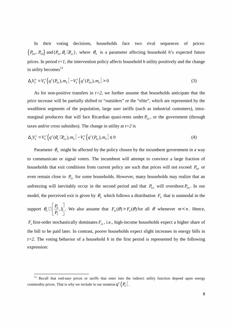
In their voting decisions, households face two rival sequences of prices:

{ }0 0, h hP P and 1 2{ , }h h hP Pθ ⋅ , where hθ is a parameter affecting household h’s expected future

prices. In period t=1, the intervention policy affects household h utility positively and the change

in utility becomes12

( ) ( )1 1 0( ), ( ), 0e e e e eh h h h h h hV V q P m V q P m∆ = − > (3)

As for non-positive transfers in t=2, we further assume that households anticipate that the

price increase will be partially shifted to “outsiders” or the “elite”, which are represented by the

wealthiest segments of the population, large user tariffs (such as industrial customers), intra-

marginal producers that will face Ricardian quasi-rents under 2hP , or the government (through

taxes and/or cross subsidies). The change in utility at t=2 is

( ) ( )2 2 1( ), ( ), 0e e e e eh h h h h h h hV V q P m V q P mθ∆ = ⋅ − ≤ (4)

Parameter hθ might be affected by the policy chosen by the incumbent government in a way

to communicate or signal voters. The incumbent will attempt to convince a large fraction of

households that exit conditions from current policy are such that prices will not exceed 0hP or

even remain close to 1hP for some households. However, many households may realize that an

unfreezing will inevitably occur in the second period and that 2hP will overshoot 0hP . In our

model, the perceived exit is given by hθ which follows a distribution hF that is unimodal in the

support 0

2

,1h

P

Pθ

∈

. We also assume that ( ) ( )m nF Fθ θ> for all θ whenever m n< . Hence,

nF first-order stochastically dominatesmF , i.e., high-income households expect a higher share of

the bill to be paid later. In contrast, poorer households expect slight increases in energy bills in

t=2. The voting behavior of a household h in the first period is represented by the following

expression:

12 Recall that end-user prices or tariffs that enter into the indirect utility function depend upon energy

commodity prices. That is why we include in our notation ( )ehq P .

9

1 2

1 2 1 2

1 2

1 if 0

Prob( , ) 1/ 2 if 0

0 if 0

e eh h

e eh h

e

h

eh h

h

V V

P P V V

V V

δδδ

∆ + ∆ >= ∆ + ∆ = ∆ + ∆ <

(5)

The previous equation gives the condition for household h to prefer { }1 2,h hP P over{ }0 0,h hP P .

The fraction of households voting for the populist policy is

( )1 2 1 2( , ) e eh h h hP P G V Vπ δ= ∆ + ∆ (6)

where we have assumed that all households have the same discount factor and that G is a smooth

cumulative distribution function with an associated density function g.

Government

Departures from opportunity cost pricing are punished during the second period for different

reasons. For instance, they affect the incentives to invest in hydrocarbon exploration or to adopt

new technologies, converting the country (led by the incumbent political party) into a high-risk

investment. If during the first period 1P is below 1C (i.e., opportunity cost), then it is very likely

that 2C will stand significantly above1C . Let us consider the following expression formalizing

this idea:

( )1 1 1t t t tC C C Pκ ε− − −= + − + (7)

where ( )κ ⋅ is a function that captures the intervention premium, i.e., the additional opportunity

cost observed in t=2 due to the effect of the populist policy implemented in t=1. The shock

ε follows a mean-zero and symmetric (around the mean) distribution. We assume that the

intervention premium is differentiable with 0κ ′ > , 0κ ′′ > , and also that (0) 0κ = . To facilitate

the analysis, let us suppose that there is an inter-temporal budget constraint and also that general

taxes (or government revenues coming from other sectors) cannot be used to subsidize energy.

For simplicity, omitting shock ε from the LRSOC transition equation, the incumbent

government solves the following maximization problem:

10

{ }

( )

1 21 2 1 2

,

1 1

11

2 2

2 1

Max ( ) ( ) ( , )

s.t. ( ) ( ) 0

e eh h h

P Ph

V P V P P P K

P C P C

C C C P

α δ θ π

δκ

∈ + ⋅ + ⋅

− + − ≥= + −

∑P

(8)

where 0α > is the weight that the politician places on total utilitarian social welfare (relative to

the weight placed on rents from being in office). The additional utility that the politician derives

from being in office is given by K. Energy prices are chosen from a set of “politically feasible”

prices, P , which might be a discrete subset or a continuum of non-negative real numbers. As we

supposed that there are no random shocks to opportunity costs in expression (7), we have

that 0 1C C= . Note also that 0 1 2C C C= = if no intervention policy is implemented.

Political equilibrium

From expression (5) presented previously, we are able to define household h’ critical discount

factor as

* 1

2

Ee

hh e

h

V

Vδ

−∆= ∆ (9)

if an interior solution for δ (between 0 and 1) exists, or else * 1hδ = . It is clear that *hδ depends

upon h because the ratio of current to future utility transfers depends on hθ , which in turn

follows a distribution hF . Thus, the value *hδ is a decreasing function of [ ]2E h hPθ ⋅ and, by

assumption, a decreasing function of income. We can therefore order households as follows:

**1 Hδ δ⋅ ⋅ >⋅> .

By combining the two restrictions in problem (8), we can transform it into an unconstrained

maximization problem since the optimal price in t=2 is a function *2 1 1( , , )P C P δ .13 For values of

α sufficiently near zero, the incumbent government is only concerned about being in office by

having a closer look to the polls. In this situation, the equilibrium prices * *1 2{ , }P P are those

13Concretely, 1* 12

1 1(1 ) ( )C C P PP

δ δ κδ

+ + − −=

11

favored by the median household (voter) and the probability of winning the election in

equilibrium is itself a function *1 1( , , )C Pπ δ .

Proposition 1. When 0α ≅ , a necessary and sufficient condition for energy populism to arise as

equilibrium is that the median household expects to receive higher gains in t=1 than losses in

t=2, or equivalently ( )*2M M MPδ δ θ≤ ⋅ where M stands for median household.

Proof: Derived from the condition that *Mδ δ> is an equilibrium.

3. Household welfare

The previous discussion motivated the analysis of the trade-off between present value gains and

losses derived from the implementation of energy populism as an equilibrium policy. In this

section, we make some effort to measure actual income transfers and their corresponding welfare

effects. We follow a simple methodology to evaluate aggregate welfare from final outcomes in

individual utility assuming some aggregation (i.e. social welfare) function. Recall from Section 2

that each household has an indirect utility function ( , )eV q m . Social welfare is represented by the

aggregation of individual utilities 1( , , )HW W V V= ⋅⋅⋅ . As explained previously, end-user prices

depend on energy-commodity prices, hP, which are the object of change and analysis.

For the empirical implementation, we make auxiliary assumptions on the shape of the social-

welfare and individual-utility functions. A simple parameterization (see for example, Newbery

[1995], and Navajas [1999])14 assumes that the social welfare function is additive in utility

levels, /hh

W U H=∑ , and that individual agents have iso-elastic utilities on consumption or real

expenditure of the type 1( ) / (1 )vh hU g v−= − for 0 v< and 1v ≠ , or log( )h hU g= for 1v = , where

hg is household h expenditure per equivalent adult, and v is interpreted as a coefficient of

inequality aversion. Under these assumptions, household h social marginal utility of income can

be computed by the expression ( ) vh hgβ −= , i.e. the inverse of expenditures per equivalent adult

14 An alternative specification that assumes a weighted welfare function of indirect utility functions arrives at

the same results without the need for specifying the form of utility functions. The adopted specification facilitates the computing of percentage welfare changes from household expenditures.

12

raised to the coefficient v. Additionally, under the assumption of an additive-cum-isoelastic-

utility specification, social welfare can be approximated by the weighted sum of expenditures per

equivalent adult, 1( )1

(1 )

vh

h

gW

H v

− = −

∑ , and the corresponding measure of relative welfare change

becomes15

h hh

h hh

gW

W g

β

β

⋅∆∆ =

⋅

∑

∑ (10)

Now suppose that a policy gives rise to a change in the vector price of energy( )ehq P , which

in turn exerts a welfare marginal impact given by the partial derivative

ehh he e

h hh h h

VW Wx

q V qβ∂∂ ∂= = −

∂ ∂ ∂∑ ∑ (11)

where h h

h

VW

V mβ ∂∂=

∂ ∂ is the social marginal utility of household h income, e

hx is the quantity of

electricity or natural gas consumed by h, and Roy’s identity has been used. Welfare impacts of

discrete changes in energy prices can be approximated by16

1 0( )eh h h h

h

W x P Pβ∆ = − −∑ (12)

Hence, we approximate the total transfer received by household h by 1 0( )heh hx P P− , the

percentage of the transfer in terms of total income as 1 0( ) /eh h h hx P P g− , the total welfare change

by (12), and the percentage welfare change using expression (10) as

15 Using the definition of ( ) v

h hgβ −= we obtain (1/ (1 )) h hh

W H v gβ= − ∑ . Thus, the percentage variation

in welfare is given by / /h h h hh h

W W g gβ β∆ = ∆∑ ∑ .

16 In expression (11), ehx can be approximated from a Taylor expansion by 0 , 1 0 0( )[1 ( ) / ]e

h x P h h hx P P P Pη+ − ,

where ,x Pη is the direct price-elasticity of demand (for electricity or natural gas). In the empirical evaluation later,

we do not exploit this loop, given that the magnitude of the jumps in prices are very large and would imply large- quantity corrections even with very low elasticity values (such as those reported for natural gas and electricity in several empirical papers).

13

1 0( )eh h h h

h

hhh

x P PW

W g

β

β

−∆ = −

∑

∑ (13)

This expression will be computed later in this study for alternative values of the income

inequality aversion coefficient, v.

4. Empirical illustration.

With the model of the previous section in mind, we now seek to measure the consequences of a

sequence of natural gas and electricity prices faced by Argentinean households during the last

decade.

4.1. The Argentinean case. An overview of the situation.

Post-2003 Argentina appears to perfectly fit in the populist model described before. Within a

policy of repressed energy prices in general, even with clear signs of cumulative imbalances in

its main energy product (i.e., natural gas) and soaring international energy prices, wholesale

markets of natural gas and electricity generation were severely intervened, entailing prices that

depart from LRSOC.17 In the case of natural gas (formerly a very competitive sector), it could

perhaps have sustained production plans with wellhead prices below the import parity (whose

relevant value is the import price from Bolivia) before the consolidation of the interventionist

regime. However, after intervention, sustainable wellhead prices were required to move toward

import prices. Although the origin and magnitudes in this example can be subject to discussion,

the important fact for the sake of our argument is their qualitative evolution: ex-post-intervention

opportunity costs are higher than ex-ante-intervention opportunity costs. Therefore, economic

agents face a net efficiency loss.

A great deal of debate in Argentina has been focused on energy subsidies in terms of their

fiscal short-run consequences. But in this paper, we look at the role of subsidies from a long-run

economic viewpoint. The difference is important because fiscal transfers made by the

government are actual disbursements to energy producers to account for the difference between 17 The term “sustainable” in LRSOC refers to the fact that there is an expansion of supply (natural gas and

electricity generation capacity) to sustain. This applies in particular to natural gas, where reserves to production have been falling and require a prompt, dynamic response. In other words, LRSOC are regarded as signals that will ensure a sustainable energy supply.

14

costs (or producer prices) and end-user prices. However, this gap does not represent the true

resource-cost gap to the economy. Economic subsidies are the difference between end-user

prices and opportunity costs represented by border prices or long-run incremental costs in the

case of tradable and nontradable goods, respectively.

4.2. Measurement

We employ different data from several sources and make some assumptions in order to

estimate household transfers and changes in welfare. The basic ingredients relate to prices and

quantities.

4.2.1. Prices

Concerning energy prices actually paid by households, we use the corresponding commodity-

price components for natural gas and electricity, which should not be mistaken for end-user

tariffs, which include transmission and distribution costs as well as advalorem taxes. Natural gas

prices were taken from ENARGAS data and include the two companies (Metrogas and Gas Ban)

serving the AMBA region. Electricity prices are seasonal, monomial prices for residential

demand taken from CAMMESA data and include the two companies serving the area (EDENOR

and EDESUR).

As for long-run sustainable opportunity costs, i.e., prices that can sustain an expansion of

supply so as to meet demand, we make different, but related, assumptions for natural gas and

electricity. In the case of natural gas, we take border prices with Bolivia as reference wellhead

prices that would sustain an expanding natural gas supply. These values were checked from

different sources, such as the unitary import prices implicit in the Secretary of Energy (SE) data18

and reference values from public and private Bolivian sources. In the case of electricity, we

assume a generation cost of a combined-cycle plant that has variable costs related with the cost

of natural gas from Bolivia and high fixed costs related with a high discount rate.

Tables A.1, A.2, and A.3 in the Appendix depict the series of actual prices, estimated

opportunity costs, and estimated subsidies of natural gas and electricity generation paid by

households in the AMBA region from 2003‒2014. The implicit subsidy in natural gas started at

1.3 U.S. dollars per million btu (USD/mmbtu) in 2003 and then moved upward, ranging from

18

Secretary of Energy has some problems concerning these values.

15

11‒13 USD/mmbtu in 2014 (according to the new differentiated tariff block structure that was

implemented from 2008). In 2003, the price actually embedded in natural gas tariffs was about

28% of the assumed opportunity cost, while in 2014 this figure had moved down to <5% for

households that faced no increases (about 60% of households) and to about 14% for households

with the largest increases. In the case of electricity, the implicit subsidy moved from 30% of

opportunity costs in 2003 to a mere 6% in 2014 for household with frozen tariffs (71% of total

households) and to 23% for households with the largest increases.

4.2.2. Quantities

Aggregate annual quantities (2003‒2014) of natural gas consumed by households in the

AMBA are taken from ENARGAS and refer to cubic meters sold to residential customers in the

Metrogas and Gas Ban areas. Aggregate annual quantities (2003‒2014) of electricity consumed

by households in the AMBA are taken from the Secretary of Energy. Adjustment in quantities in

response to increases in prices after 2014 (stated as the figurative year 201X) were not estimated

with a price-elasticity of demand, but is rather assumed as a sensitivity analysis for different

cases (see below).

Quantities used for the evaluation of incidence and welfare impact of household transfers

were taken from the National Household Expenditure Survey for the AMBA. Following a

method used in Navajas (2009), we were able to retrieve the quantities of natural gas and

electricity consumed by each household in the survey. We are therefore able to implement the

formulas of the previous section from observed quantities. We also use the distribution of

consumptions across households, along with household data on income and total expenditure,

which allows us to compute the social marginal-income utility of each household in order to

implement the welfare weights vh hgβ −= of the previous section.

4.2.3. Household transfers

Subsidies received by households during 2003‒2014 are measured by ( )1 0eh h hx P P⋅ − in the

expressions of the previous section, where ehx is the quantity of natural gas or electricity

consumed by household h and ( )1 0h hP P− is the unit subsidy (the difference between actual prices

and opportunity costs) estimated in Tables A.1, A.2, and A.3 as mentioned previously.

16

Tables 1 and 2 present the estimates of household transfers for natural gas and electricity.

Numbers are expressed in millions of U.S. dollars (USD) per year for each decile of income

(arranged according to per-capita household income) and separated into the periods of full freeze

(2003‒2007), partial adjustment (2008‒2014), and a hypothetical return to full-cost pricing (in

the figurative year 201X) under two assumptions of no demand correction (i.e.. valuated at the

same quantities) and a 10% demand correction. The difference between the subsidy periods

(2003‒2007 and 2008‒2014) and the full-adjustment period is that while the former are actual

estimates for a given period, the latter is a hypothetical estimation of an annual flow in the

future.

Table 1. Natural Gas: Estimated Annual Transfers to Households in the Metropolitan Region of Buenos Aires (in millions of U.S. Dollars)

Decile

Estimated transfers for sub-period

Without demand correction

10% demand correction

2003-07 2008-13 201X? 201X? 1 10.3 41.0 -58.9 -53.0 2 17.7 67.8 -99.0 -89.1 3 21.7 82.7 -121.0 -108.9 4 26.0 98.3 -144.0 -129.6 5 31.5 116.8 -173.6 -156.2 6 37.5 138.4 -206.1 -185.5 7 40.8 146.1 -221.2 -199.1 8 44.5 159.7 -242.3 -218.1 9 45.0 159.8 -244.8 -220.4 10 44.1 152.3 -239.8 -215.8

Total 319.3 1163.0 -1750.8 -1575.8 Source: own elaboration based on ENGH 2004-2005

Table 2. Electricity: Estimated Annual Transfers to Households in the Metropolitan Region of Buenos Aires (in millions of U.S. Dollars)

Decile Estimated transfers for sub-period

Without demand correction

10% demand correction

2003-07 2008-14 201X? 201X? 1 24.9 67.9 -87.1 -78.4 2 30.1 82.7 -105.7 -95.1 3 36.2 98.2 -126.1 -113.5 4 35.1 96.4 -123.0 -110.7 5 36.6 99.3 -127.1 -114.4

17

6 39.1 107.0 -136.2 -122.6 7 39.7 108.7 -138.2 -124.4 8 40.3 109.4 -139.6 -125.6 9 42.7 116.1 -147.5 -132.7 10 49.3 132.5 -168.4 -151.6

Total 373.9 1018.3 -1299.0 -1169.1 Source: own elaboration based on ENGH 2004-2005

Total transfers, from 2003‒2014, to households in the Buenos Aires Metropolitan Region

amounted to 19.3 billion USD (i.e., somewhat >1.6 billion USD per year). This is, on average,

on the order of 0.3% of GDP per year. Under-pricing of electricity generation caused somewhat

more subsidies than underpricing of natural gas. Despite the correction in 2008 to some

households, actual subsidies rose due to a significant rise in opportunity costs that are related

with international energy prices and with the restricted nature of price increases. As there are

about 4 million households in this area, each household received, on average, an equivalent

annual subsidy of about 400 USD. But the distribution of the subsidies, given the uniform prices

until 2008, was not pro-poor- or pro-low-income households. Rather, it benefited the higher

deciles of income distribution to a relatively greater degree (see Table 3). This is not surprising

given the fact that subsidies were uniform and proportional to consumption until 2008. In the

case of natural gas, the unfair distribution against low-income households is compounded by the

fact that many of these do not receive any subsidy because they are not connected to the natural

gas network (see Table A.4 in the Appendix) and use liquefied petroleum gas (LPG) at

opportunity cost values. Hence, the nearly 4:1 ratio in 2003‒2014 subsidies received by the 10th

compared to the 1st decile can be explained by a 1.5:1 ratio in average consumption and by a 3:1

ratio in access to the network.

Table 3. Distribution of natural gas and electricity subsidies across households between 2003 and 2014

Decile Natural Gas Electricity Total 1 3.5% 6.7% 5.0% 2 5.8% 8.1% 6.9% 3 7.1% 9.6% 8.3% 4 8.4% 9.4% 8.9% 5 10.0% 9.8% 9.9% 6 11.9% 10.5% 11.2%

18

7 12.6% 10.7% 11.7% 8 13.8% 10.8% 12.3% 9 13.8% 11.4% 12.6% 10 13.2% 13.0% 13.1%

Source: Tables 1 and 2

A return to opportunity cost is a reversion of subsidies that will imply transfers in opposite

directions to those observed in 2003‒2014. Annual transfers will depend on demand correction

but will surely –and given higher projected natural gas prices that exert an impact on both

estimates- be of a magnitude of about 2.7 billion USD per year (or >0.45% of current GDP), a

large figure considering that we are measuring only households in the Buenos Aires

Metropolitan Region, which means about 25% percent of total consumption of natural gas and

electricity. Unlike the transfers in 2003‒2014, these will imply a permanent flow with a

correspondingly large amount in relation to the “floor” at which prices were at the end of the

subsidy era.

4.2.4. Welfare impacts

Tables 4 and 5 present the estimated annual percentage welfare changes (expression (13)) for

the two different sub-periods and for different degrees of inequality aversion (v = .5, 1, and 2).

Again, we assume a 10% demand correction after prices return to opportunity cost pricing in

201X. The results show significant changes in welfare for households, but in particular for low-

income ones. The impact of household transfers on welfare is (as expected) a decrease in

income. Recall that changes in welfare depend on the income level of each household, along

with the degree of inequality aversion. Thus, the distribution of welfare gains has a higher impact

on the poor, a fact that is only seemingly contradictory to the evidence that a large amount of

subsidies go to the non-poor. The reason is that large subsidies for the wealthy are not as

significant in terms of social welfare as those received by the poor.

Table 4. Natural Gas: Average Annual Percentage Change in Welfare

Decile Aversion coefficient (v=.5) Aversion coefficient (v=1) Aversion coefficient (v=2) 2003-07 2008-14 201X? 2003-07 2008-14 201X? 2003-07 2008-14 201X?

1 1.9% 7.3% -8.7% 2.1% 7.9% -9.3% 2.6% 10.0% -11.7% 2 1.3% 4.8% -5.8% 1.3% 4.9% -5.8% 1.3% 4.9% -5.9% 3 1.0% 3.6% -4.3% 1.0% 3.6% -4.3% 1.0% 3.6% -4.3%

19

4 0.8% 2.9% -3.5% 0.8% 3.0% -3.5% 0.8% 3.0% -3.6% 5 0.7% 2.7% -3.2% 0.7% 2.7% -3.2% 0.7% 2.7% -3.3% 6 0.6% 2.3% -2.8% 0.6% 2.3% -2.8% 0.6% 2.3% -2.8% 7 0.6% 2.1% -2.6% 0.6% 2.1% -2.6% 0.6% 2.1% -2.6% 8 0.5% 1.6% -2.0% 0.5% 1.6% -2.0% 0.5% 1.6% -2.0% 9 0.4% 1.3% -1.6% 0.4% 1.3% -1.6% 0.4% 1.3% -1.6% 10 0.2% 0.8% -1.0% 0.2% 0.8% -1.1% 0.3% 0.9% -1.1%

Total 0.5% 2.0% -2.4% 0.7% 2.5% -3.1% 1.2% 4.4% -5.3% Note: Assumes a uniform 10% demand correction during the populist cycle reversion (i.e. year 201X?)

One important element of the results illustrated in Tables 4 and 5 is that (for the very same

reason that percentage welfare impacts on the poor are large), the variability of the impacts is

correspondingly large. To the extent that subsidies will be followed by price hikes, the wealthiest

households will face variability in welfare of a relatively small magnitude, while the poorest will

experience a great swing in utility and welfare.

Table 5. Electricity: Average Annual Percentage Change in Welfare

Decile Aversion coefficient (v=0.5) Aversion coefficient (v=1) Aversion coefficient (v=2) 2003-07 2008-14 201X? 2003-07 2008-14 201X? 2003-07 2008-14 201X?

1 1.9% 4.6% -5.0% 2.0% 5.0% -5.5% 3.1% 7.6% -8.3% 2 1.1% 2.8% -3.1% 1.2% 2.9% -3.1% 1.2% 2.9% -3.2% 3 1.0% 2.5% -2.8% 1.0% 2.5% -2.8% 1.0% 2.5% -2.8% 4 0.8% 2.0% -2.2% 0.8% 2.0% -2.2% 0.8% 2.0% -2.2% 5 0.7% 1.7% -1.9% 0.7% 1.7% -1.9% 0.7% 1.7% -1.9% 6 0.6% 1.5% -1.6% 0.6% 1.5% -1.6% 0.6% 1.5% -1.6% 7 0.5% 1.3% -1.4% 0.5% 1.3% -1.4% 0.5% 1.3% -1.4% 8 0.4% 1.1% -1.2% 0.4% 1.1% -1.2% 0.4% 1.1% -1.2% 9 0.4% 0.9% -1.0% 0.4% 0.9% -1.0% 0.4% 0.9% -1.0% 10 0.3% 0.6% -0.7% 0.3% 0.7% -0.7% 0.3% 0.7% -0.8%

Total 0.6% 1.4% -1.6% 0.8% 1.9% -2.1% 1.6% 3.9% -4.3% Note: Assumes a uniform 10% demand correction during the populist cycle reversion (i.e. year 201X?)

5. Conclusion

In this study we adopt the term “energy populism” to characterize a class of unsustainable

pricing policies observed in some developing economies in the last decade (e.g. recent

experiences in Argentina, Iran and Armenia). To our knowledge, we are the first to provide an

20

analytical framework for explaining the emergence of the energy populism in terms of the

preferences of a median household (i.e. voter) for receiving transfer gains followed by a stream

of transfer losses. This description depends on a critical discount factor that in turn is contingent

upon on a perception that the transfer losses will be somehow shifted away.

From theoretical grounds, a suggested line of future research is to polish the strategic

behavior of the incumbent to implement (and of society to vote for) energy populism. In

particular, exploring the inconsistencies involved in choosing the populist path given that

consequences may end up being quite different from discourse or narrative, is an interesting

topic. Another possible extension is the interplay between the adoption of energy populism and

the policy-technology for dealing with transfers, particularly the lack of incentives to target

energy subsidies to the poorest households accurately. Exit conditions from heavily subsidized

prices poses a problem for society, given that at the new energy prices, a larger proportion of

agents will encounter serious difficulties in coping with the energy price shocks.

Our empirical illustration is also original insofar as it characterizes transfers and welfare

effects, clarifying the apparent puzzling or conflicting properties embedded in assertions about

energy subsidies; i.e. they are usually termed “progressive” and “pro-rich” at the same time. This

is so because the standard incidence test (where subsidies are progressive if they are decreasing

in income, as a percentage of household income) is used to assert the former, while the

measurement of the share of the non-poor in total subsidies is used to assert the latter. To

complete the assessment we use an explicit measurement framework that allow us to deal with

the welfare effects of the full subsidy cycle, dealing not only with levels but also with welfare

instability induced by unsustainable subsidy policies. We show that the percentage instability of

welfare experienced by households is decreasing in income, this effect being larger the higher

the degree of inequality aversion, adding another dimension to the distributive characterization

of energy subsidies policies.

Our empirical research is based on the Argentinean case during the last decade. This country

embarked on an interventionist energy policy, particularly concerning wholesale natural gas and

electricity markets. This interventionism led to what is perhaps the largest tariff freeze in history,

particularly for households in the Buenos Aires Metropolitan Region, about 40% of the country’s

population and the historical stronghold of supporters of redistributive politics. If prices were

21

below opportunity costs at the beginning of the freeze in 2002, the two astonishingly became

divorced from 2003 on as international energy prices rose. The presence of visible imbalances

did not trigger policy response up until 2008, as world energy prices soared. But the response

was carefully designed to avoid being perceived as a policy reversal. Contrariwise, energy policy

in Argentina became quite committed to the freeze or to real deterioration (as inflation picked up

since 2007) for a significant percentage of households (with low-to-medium consumption

levels). This was costly, accomplished as it was through a multi-part tariff schedule that left

many holes, in particular in terms of inclusion errors (i.e., upper-middle-class or wealthy families

with low-to-medium consumption levels included in the subsidy scheme).

On evaluating long-run sustainable opportunity costs at what we think are reasonable scarcity

values for Argentina, we found that about 4 million households in the Metropolitan Region of

Buenos Aires (about 40% of the population) received in total >19 billion U.S. dollars (USD) in

subsidies between 2003 and 2014, or in annual terms, about 0.3% of the (average) GDP of that

period. The distributive incidence of these transfer gains is very weak, particularly for the case of

natural gas, as incomplete access to the network means that 40% of the poorest 50% of

households do not have natural gas and buy LPG at opportunity costs. For both natural gas and

electricity, distribution of subsidies is significantly biased toward the non-poor, because the share

in the total subsidies of the wealthiest 20% of households is more than double that of the poorest

20%.

Welfare impacts for society as a percentage of total welfare are quite significant for both

natural gas and electricity. As expected, percentage welfare gains for the poorest households are

considerable larger compared with equivalent gains for the wealthy, due to the large differences

in income.

We do not elaborate on the transition from subsidized prices to a new equilibrium. This move

has partially begun, albeit slowly and with difficulties, due to the poor targeting associated with

multi-part prices that implemented large price hikes for a small group of large consumers. We

make a simple calculation of transfer losses on the assumption that the gap is closed and that

every household pays opportunity costs. These are distributed in a similar fashion as transfer

gains, given the assumed proportional (to consumption) adjustment for all households. However,

the same is true with percentage welfare losses, that is, the poor receive the largest negative

22

impacts. Thus, subsidy cycles have an additional property that is usually neglected in their

distributional assessment, namely that they give rise to a larger welfare instability for the poor

than for the non-poor.

From the previous results, it is clear that one drawback of following interventionist policies is

the transmission of income and welfare instability to the society and, in particular, the poor.

What more can we say based on our measurement of AMBA household subsidies concerning the

costs of energy populism? The answer depends on auxiliary assumptions, in particular on what

can be said regarding the magnitude and duration of excess costs to be borne as a consequence of

a decade of interventionism. While it is clear that the energy bill for the household sector in

Argentina will increase substantially, the proper “excess cost” borne by households is the

“premium” that Argentina managed before embarking on energy populism, such as enjoying a

competitive up-stream natural gas sector that could sustain supply with prices below border

prices. For example, assuming that this gap is only 20% of the computed jump from current

prices to opportunity cost values, and a discount rate of 5%, the present value of the excess cost

borne by households in the AMBA can be estimated at about 6 billion USD, or >1.3% of the

current GDP.

References

Acemoglu, D., Egorov, G., and Sonin, K. (2012). A Political Theory of Populism. The Quarterly Journal of Economics

Angel-Urdinola, D., and Wodon, Q. (2007). Do Utility Subsidies Reach the Poor? Framework and Evidence for Cape Verde, Sao Tome, and Rwanda. Economics Bulletin, Vol. 9(4)

Artana, D., Catena, M., and Navajas, F. (2007). El Shock de los Precios del Petróleo en América Central: Implicancias Fiscales y Energéticas. Working Paper WP 624, Research Department, Inter-American Development Bank

Bacon, R., and Kojima, M. (2006). Coping with Higher Oil Prices. ESMAP Report 323/06, World Bank

Borenstein, S. (2010).The Re-distributional Impact of Non-Linear Electricity Pricing. NBER Working Paper 15822

Bour, E., Heymann, D., and Navajas, F. (2004). Latin American Macroeconomic Crisis, Trade and Labor.London: Macmillan

Canitrot, A. (1975). La Experiencia Populista de Redistribución de Ingresos. Desarrollo Económico, Vol. 15(59): pp. 331-351

23

Clements B., D, Coady, S. Frabrizio, S. Gupta, T. Alleyne, and C. Sdralevich (2013). Energy Subsidy Reform: Lessons and Implications, Washington D.C.: International Monetary Fund, Washington, D.C., 2013

Coady D., I. Parry, L. Sears, and B. Shang (2015). How Large are Global Energy Subsidies?, Working Paper WP/15/105, International Monetary Fund

Cremer, H., De Donder, P., and Gahvari, F. (2008). Energy Taxes in Three Political Economy Models, B.E. Journal of Economic Analysis & Policy, Vol. 7(32)

Dornbusch, R. and Edwards, S. (1991). The Macroeconomics of Populism in Latin America, The University of Chicago Press

Edwards, S. (2010). Left Behind: Latin America and the False Promise of Populism. University of Chicago Press

Greenpeace (2013). Submission to the Ad Hoc Working Group on the Durban Platform for Enhanced Action Regarding Views on Options and Ways for Further Increasing the Level of Ambition. Link: http://unfccc.int/resource/docs/2012/smsn/ngo/135.pdf

Izquierdo, A., Loo-Kung, R., and Navajas, F. (2013). Resistiendo el canto de las sirenas financieras en Centroamérica: una ruta hacia un gasto más eficiente con crecimiento, Banco Interamericano de Desarrollo:

http://idbdocs.iadb.org/wsdocs/getdocument.aspx?docnum=38196681

Jorgenson, D. (1997). Welfare - Vol. 1.Aggregate Consumer Behavior. MIT Press

Laclau, E. (2005). On Populist Reason. London: Verso

Marchioni, M., Sosa-Escudero, W., and Alejo, J. (2008). Efectos distributivos de esquemas alternativos de tarifas sociales: una exploración cuantitativa. Ch. 2 in Navajas (2008) op. cit.

Mendoza, M.A (2014). Panorama preliminar de los subsidios y los impuestos a las gasolinas y diésel en los países de América Latina, LC/W.641, UN Economic Commission for Latin America and the Caribbean, Santiago de Chile

Navajas, F. (1999). Structural Reforms and the Distributional Effects of Price Changes in Argentina. SSRN Working Paper

Navajas, F. (2006). Estructuras Tarifarias Bajo Stress. Económica (La Plata), (Núm. 1-2): pp. 77-102

Navajas, F. (2008). La Tarifa Social en los Sectores de Infraestructura en la Argentina. Grupo Editorial TEMAS

Navajas, F. (2009). Engel Curves, Household Characteristics and Low-user Tariff Schemes in Natural Gas. Energy Economics, Vol. 31(1): pp. 162-168

Navajas, F. (2015). Energy Subsidies Revisited, 5th Latin American Energy Economics Meeting, Medellin, Colombia, http://www.aladee.org/index_en.html

Newbery, D. (1995). The Distributional Impact of Price Changes in Hungary and the United Kingdom. Economic Journal, Vol. 105: pp. 847-863

ODI (2013). Time to Change the Game: Fossil Fuels, Subsidies and Climate. Overseas Development Agency, London

24

OECD (2012). Energy Subsidies, International Energy Agency. Access through link: http://www.worldenergyoutlook.org/resources/energysubsidies/

UNFCC (2013). Warsaw Climate Change Conference November 2013. Access through link: http://unfccc.int/meetings/warsaw_nov_2013/meeting/7649.php

Persson, T., and Tabellini, G. (2002). Political Economics: Explaining Economic Policy. MIT Press

Plante M. (2014). The Long-run Macroeconomic Impacts of Fuel Subsidies, Journal of Development Economics, Vol. 107: pp. 129-143

Vagliasindi, M. (2012). Implementing energy subsidy reforms: Evidence from developing countries. World Bank Publications.

Woods, D. (2014). The Many Faces of Populism: Diverse but not Disparate,

Research in Political Sociology, Volume 22, pp. 1-25

World Bank (2010). Subsidies in the Energy Sector: An Overview, Background Paper for the World Bank Group Energy Sector Strategy, Washington, D.C. July

25

Appendix

Table A.1 Metrogas. Residential Natural Gas: Commodity Gas Price (in U.S. Dollars / mmBtu)

Year m3 / year Oportunity

cost Price included in tariff Implicit Subsidy

Bs As City Greater Bs As Bs As City Greater Bs As 2003 > 0 1.78 0.47 0.49 1.31 1.29 2004 > 0 1.78 0.44 0.47 1.34 1.31 2005 > 0 2.81 0.38 0.44 2.43 2.37 2006 > 0 3.87 0.36 0.41 3.51 3.46 2007 > 0 5.16 0.35 0.41 4.81 4.75 2008 0 - 800 8.54 0.35 0.40 8.19 8.14

801 - 1000 8.54 0.39 0.43 8.15 8.11 1001 - 1250 8.54 0.49 0.53 8.05 8.01 1251 - 1500 8.54 0.55 0.59 7.99 7.95 1501 - 1800 8.54 0.66 0.71 7.88 7.83 1801 - more 8.54 0.72 0.77 7.82 7.77

2009 0 - 800 5.88 0.30 0.34 5.58 5.53 801 - 1000 5.88 0.39 0.41 5.49 5.47 1001 - 1250 5.88 0.88 0.91 4.99 4.96 1251 - 1500 5.88 1.24 1.27 4.63 4.60 1501 - 1800 5.88 2.00 2.05 3.88 3.83 1801 - more 5.88 2.42 2.46 3.46 3.41

2010 0 - 800 7.27 0.28 0.33 6.99 6.95 801 - 1000 7.27 0.37 0.39 6.90 6.88 1001 - 1250 7.27 0.84 0.87 6.43 6.40 1251 - 1500 7.27 1.18 1.21 6.09 6.06 1501 - 1800 7.27 1.91 1.95 5.37 5.32 1801 - more 7.27 2.30 2.35 4.97 4.92

2011 0 - 800 10.85 0.27 0.32 10.58 10.54 801 - 1000 10.85 0.36 0.38 10.50 10.48 1001 - 1250 10.85 0.80 0.83 10.05 10.02 1251 - 1500 10.85 1.14 1.17 9.71 9.68 1501 - 1800 10.85 1.84 1.88 9.02 8.98 1801 - more 10.85 2.22 2.27 8.63 8.59

2012 0 - 800 13.18 0.28 0.32 12.90 12.86 801 - 1000 13.18 0.36 0.38 12.81 12.80 1001 - 1250 13.18 0.76 0.79 12.41 12.39 1251 - 1500 13.18 1.13 1.16 12.05 12.02 1501 - 1800 13.18 1.83 1.87 11.34 11.30 1801 - more 13.18 2.26 2.30 10.92 10.88

2013 0 - 800 13.40 0.23 0.26 13.17 13.14 801 - 1000 13.40 0.30 0.32 13.10 13.08 1001 - 1250 13.40 0.63 0.66 12.77 12.74

26

1251 - 1500 13.40 0.94 0.96 12.46 12.44 1501 - 1800 13.40 1.53 1.56 11.87 11.84 1801 - more 13.40 1.88 1.91 11.52 11.49

2014 651 - 800 13.65 0.34 0.34 13.32 13.31 801 - 1000 13.65 0.45 0.46 13.20 13.20 1001 - 1250 13.65 0.83 0.84 12.82 12.82 1251 - 1500 13.65 1.14 1.14 12.51 12.51 1501 - 1800 13.65 1.66 1.67 11.99 11.98 1801 - more 13.65 2.22 2.22 11.44 11.43 Source: Own elaboration as explained in the text. Data from ENARGAS and Secretary of Energy and CBDH for Bolivian gas.

Table A.2. GasBan. Residential Natural Gas: Commodity Gas Price (USD / MMBTU)

Year m3 / year Oportunity cost Price included in tariff Implicit Subsidy

Greater Bs As Greater Bs As 2003 > 0 1.78 0.51 1.27 2004 > 0 1.78 0.50 1.28 2005 > 0 2.81 0.49 2.31 2006 > 0 3.87 0.47 3.40 2007 > 0 5.16 0.46 4.70 2008 0 - 800 8.54 0.49 8.05

801 - 1000 8.54 0.51 8.03 1001 - 1250 8.54 0.62 7.92 1251 - 1500 8.54 0.68 7.86 1501 - 1800 8.54 0.80 7.74 1801 - more 8.54 0.86 7.68

2009 0 - 800 5.88 0.39 5.49 801 - 1000 5.88 0.43 5.44 1001 - 1250 5.88 0.94 4.93 1251 - 1500 5.88 1.30 4.57 1501 - 1800 5.88 2.09 3.78 1801 - more 5.88 2.51 3.37

2010 0 - 800 7.27 0.37 6.90 801 - 1000 7.27 0.41 6.86 1001 - 1250 7.27 0.90 6.37 1251 - 1500 7.27 1.24 6.03 1501 - 1800 7.27 2.00 5.28 1801 - more 7.27 2.39 4.88

2011 0 - 800 10.85 0.36 10.50 801 - 1000 10.85 0.40 10.46 1001 - 1250 10.85 0.86 9.99 1251 - 1500 10.85 1.20 9.66 1501 - 1800 10.85 1.92 8.94

27

1801 - more 10.85 2.31 8.55 2012 0 - 800 13.18 0.35 12.82

801 - 1000 13.18 0.40 12.78 1001 - 1250 13.18 0.81 12.36 1251 - 1500 13.18 1.18 12.00 1501 - 1800 13.18 1.91 11.27 1801 - more 13.18 2.33 10.84

2013 0 - 800 13.40 0.29 13.11 801 - 1000 13.40 0.33 13.07 1001 - 1250 13.40 0.68 12.72 1251 - 1500 13.40 0.98 12.42 1501 - 1800 13.40 1.59 11.81 1801 - more 13.40 1.94 11.46

2014 0 - 800 13.65 0.41 13.25 801 - 1000 13.65 0.52 13.14 1001 - 1250 13.65 0.93 12.72 1251 - 1500 13.65 1.25 12.40 1501 - 1800 13.65 1.78 11.88 1801 - more 13.65 2.37 11.28

Source: Own elaboration as explained in the text. Data from ENARGAS and Secretary of Energy and CBDH for Bolivian gas.

Table A.4. Access to natural gas and electricity across households in AMBA

Decile Natural gas Electricity 1 36.6% 85.2% 2 50.1% 91.3% 3 62.0% 96.2% 4 68.9% 97.4% 5 77.6% 98.0% 6 85.7% 99.2% 7 84.6% 100.0% 8 94.4% 100.0% 9 95.7% 100.0% 10 98.0% 100.0%

Total 75.3% 96.7% Source: own elaboration based on ENGH 2004–2005.