www.eprg.group.cam.ac.uk

A Unit Commitment and Economic Dispatch Model of the GB Electricity Market – Formulation and Application to Hydro Pumped Storage EPRG Working Paper 1924

Cambridge Working Paper in Economics 1968

Chi Kong Chyong, David Newbery, and Thomas McCarty Abstract We present a well calibrated unit commitment and economic dispatch model of the GB electricity market and applied it to the economic analysis of the four existing hydro pumped storage (PS) stations in GB. We found that with more wind on the system PS arbitrage revenue increases: with every percentage point (p.p) increase in wind capacity the total PS arbitrage profit increases by 0.21 p.p.. However, under a range of wind capacity, the PS’ modelled revenue from price arbitrage is not enough to cover their ongoing fixed costs. Analysing the 2015-18 GB balancing and ancillary services data suggests that PS stations were not active in managing transmission constraints and in fact about 60% of constraint payments went to gas-fired units. However, the PS stations are active in provision of ancillary services such as fast reserve, response and other reserve services with a combined market share of at least 30% in 2018. Stacking up the modelled revenue from price arbitrage with the 2018 balancing and ancillary services revenues against the ongoing fixed costs suggests that the four existing PS stations are profitable. Most of the revenue comes from balancing and ancillary services markets – about 75% – whereas only 25% comes from price arbitrage. However, the revenues will not be enough to cover capex and opex of a new 600 MW PS station. The gap in financing will have to come from balancing and ancillary services market opportunities and less so from purely price arbitrage. Finally, we found that the marginal contribution of most of the existing PS stations to gas and coal plant profitability is negative, while from the system point of view, PS stations do contribute to minimizing the total operating cost. Keywords economic modelling; unit commitment; economic dispatch; electricity market modelling; hydro pumped energy storage; wind energy; solar energy; electrical energy storage investment JEL Classification C61; C63; L94; L98; Q40; Q41; Q48

Contact k.chyong@jbs.cam.ac.uk Publication July 2019 Financial Support Energy Policy Forum, Energy Policy Research Group

1

A Unit Commitment and Economic Dispatch Model of the GB Electricity Market – Formulation and Application to Hydro Pumped Storage

Chi Kong Chyong1, David Newbery2, and Thomas McCarty3

July 11, 2019

Abstract We present a well calibrated unit commitment and economic dispatch model of the GB electricity market and applied it to the economic analysis of the four existing hydro pumped storage (PS) stations in GB. We found that with more wind on the system PS arbitrage revenue increases: with every percentage point (p.p) increase in wind capacity the total PS arbitrage profit increases by 0.21 p.p.. However, under a range of wind capacity, the PS’ modelled revenue from price arbitrage is not enough to cover their ongoing fixed costs. Analysing the 2015-18 GB balancing and ancillary services data suggests that PS stations were not active in managing transmission constraints and in fact about 60% of constraint payments went to gas-fired units. However, the PS stations are active in provision of ancillary services such as fast reserve, response and other reserve services with a combined market share of at least 30% in 2018. Stacking up the modelled revenue from price arbitrage with the 2018 balancing and ancillary services revenues against the ongoing fixed costs suggests that the four existing PS stations are profitable. Most of the revenue comes from balancing and ancillary services markets – about 75% – whereas only 25% comes from price arbitrage. However, the revenues will not be enough to cover capex and opex of a new 600 MW PS station. The gap in financing will have to come from balancing and ancillary services market opportunities and less so from purely price arbitrage. Finally, we found that the marginal contribution of most of the existing PS stations to gas and coal plant profitability is negative, while from the system point of view, PS stations do contribute to minimizing the total operating cost.

Keywords: economic modelling; unit commitment; economic dispatch; electricity market modelling; hydro pumped energy storage; wind energy; solar energy; electrical energy storage investment

JEL classification: C61; C63; L94; L98; Q40; Q41; Q48

1 Corresponding author. Research Associate and Director of Energy Policy Forum, EPRG, Cambridge Judge Business School, University of Cambridge, email: k.chyong@jbs.cam.ac.uk 2 Emeritus Professor of Economics at the Faculty of Economics and Director of EPRG, University of Cambridge 3 Research Assistant at EPRG (from Sept-2017 until Mar-2018), University of Cambridge

2

Table of Contents Abstract ................................................................................................................................................................. 1 1. Introduction .................................................................................................................................................... 3

2. Literature Review .......................................................................................................................................... 4 2.1. Top-down and bottom-up modelling approaches .................................................................................. 4

2.2. Bottom-up modelling of an electricity system – unit commitment and economic dispatch .................. 5 3. Formulation .................................................................................................................................................... 7

3.1. Notation ....................................................................................................................................................... 7 3.2. Equations ................................................................................................................................................... 10

3.2.1 Objective function ............................................................................................................................... 10 3.2.2 System constraints .............................................................................................................................. 11

3.2.3. Thermal generation constraints .......................................................................................................... 11 3.2.4. Unit commitment constraints ............................................................................................................. 12

3.2.5. Energy Storage Constraints ................................................................................................................ 13 3.2.6. Interconnector Flows Constraints ...................................................................................................... 13

3.3. Optimization routines ................................................................................................................................ 13 3.3.1. Implementing a rolling horizon .......................................................................................................... 13

4. Application: A GB Unit Commitment and Economic Dispatch Model ....................................................... 15 4.1. Motivation ........................................................................................................................................... 15

4.2. Data input and assumptions ................................................................................................................ 16 4.2.1. Generation technologies modelled ............................................................................................. 16

4.2.2. Time horizon and granularity ..................................................................................................... 16 4.3. Calibration ........................................................................................................................................... 17

4.4. Sensitivity analysis .............................................................................................................................. 20 4.4.1. Impact of modelling horizon length on results and solution time ................................................... 20

4.4.2. Operating reserve and fast-ramping generation units ..................................................................... 23 4.4.3. Plant flexibility and commitment .................................................................................................... 26

4.5. A case study: a simple economic analysis of hydro pumped storage .................................................. 31 5. Conclusions .................................................................................................................................................. 38

6. References .................................................................................................................................................... 41 Appendix 1: Data Input and Assumptions for the GB electricity market ............................................................. 47

A.1 Notation for data inputs and parameters .................................................................................................... 47 A.2 GB electricity demand ............................................................................................................................... 47

A.3. Operating reserve requirements ................................................................................................................ 48 A.4. Dispatchable fossil fuel plant dataset ....................................................................................................... 50

A.5. Pumped Hydro Storage in GB .................................................................................................................. 53 A.6. Interconnectors ......................................................................................................................................... 53

A.7. Other costs ................................................................................................................................................ 54 Appendix 2: Detailed modelling results ............................................................................................................... 56

3

1. Introduction This paper describes a simple unit commitment (UC) model that can be rapidly

calibrated for an electricity system and used to study the impacts of varying levels of renewable electricity supply. Its distinctive features are that it handles a reasonable range of generation technologies at plant or unit level and hydro pumped storage capability at an hourly dispatch resolution while keeping the solution time on a PC to manageable times (about 10-20 minutes to solve for a time horizon of one calendar year) so that it can explore a range of fuel and carbon prices and levels of renewable penetration. Its advantage over existing more sophisticated commercial models is that it is cheap, fast to solve, and less impenetrable than more complex black box models as more simulations can be carried out to understand better the drivers of the often rather counter-intuitive results.

Modern societies depend heavily on reliable and affordable energy for social and economic development. As such, understanding the various features of energy systems that influence the markets, and the supply and demand of energy is of interest to international bodies, governments, and private sector companies. In the second half of the twentieth century, the supply and demand of energy changed dramatically, as a result of the switch of generation from coal to oil, nuclear and then gas in response to technical change and geopolitical events such as the oil crises of the 1970’s. In the electricity supply industry, restructuring, liberalization, often accompanied by privatization, and widespread decentralisation was started in Europe by the UK in the 1990’s and then adopted more widely from 1994 (Newbery, 2001). Energy systems modelling became increasingly important to understand the impact of new technologies like wind and solar PV, and support economists and governments in designing policies to meet the growing climate change challenge.

While planning models for investment decisions in centralised electricity systems are not new, the increasing emphasis on global sustainability, climate change and environmental impacts, require models to include new capabilities. Models are called on to investigate the effects of climate-focussed policies on changes made to energy pricing (e.g., HM Government, 2010; Spataru et al., 2013; Strachan, 2010). Other research investigates the role that certain technologies will play in meeting decarbonisation targets (e.g., Pye et al., 2017; Denholm et al., 2013). While it is costly and/or difficult to decarbonise heating, industry and transport, it is relatively simple to decarbonise electricity, as low-carbon technologies are available and the final product needs no change (CCC, 2016; Pfenninger et al., 2014; MIT Energy Initiative, 2016). Consequently, electricity systems modelling is a key area within the wider energy systems modelling domain and considered by Pfenninger et al. (2014) as one of the four main pillars of twenty-first century’s energy system models.

Electricity has specific characteristics that require a careful choice of modelling approach. First, supply (including from storage and imports) must equal demand at each moment and at each location. That requires the ability to control and rapidly vary output. Second, physical constraints are important, whether in generation or transmission capacity. Third, it is costly to start and stop fossil generators and may require minimum up and down-times. Taken together, minimizing system cost means taking a sufficiently long-time horizon over which plant output can be varied to minimize cost over the whole period. The model should satisfy all the physical (and other) constraints representing the operations of a real electricity system. Standard linear programming techniques cannot handle the non-

4

convexities of plant operation (start-up costs, minimum commitment time, falling average costs), and at the least mixed integer linear programs (MILP) are needed to model and understand the operation of an efficiently dispatched electricity system.

The MILP make use of well-studied search algorithms to identify feasible optimal solutions. In the case of an electricity system, feasibility is determined by the operational limits of the various generators – for example, their maximum capacity and speed of increasing output. The optimal solution is the configuration of generation that meets demand at every moment at least-cost over a suitable time period. Within the model, assumptions are made about demand levels, plant operating costs, and when they are available. The optimisation routines can be solved over varying periods, from days, to weeks, to years to identify the most cost-effective method of meeting demand.

By formulating the program with a set of constraints that respect each of the requirements of the system (e.g., demand, reserve, emissions, technology limits), the optimum dispatch and generating mix can be found for a specified future electricity system which may be quite different from the existing system, with a much higher penetration of variable renewable electricity (VRE). A good model can be used to investigate market design changes (e.g. capacity markets, new ancillary service markets, different low-carbon contracts) needed to support possible future low carbon generation scenarios.

This paper has two practical objectives. First, we want to formulate and apply a standard unit commitment (UC) model to a real market context – the GB electricity market. Second, as demonstration case studies, we used the model to analyse the: (a) the impact of a carbon tax on the CO2 emissions reduction of wind (see Chyong et al., 2019), (b) role of operational flexibility and merit order on gas power with CCS (see Schnellmann et al., 2018), (c) economics of existing hydro pumped storage (PS) (see §4.5 of this paper). The rest of our paper is organised as follows. The next section provides a literature review. Section 3 describes the UC model, followed by its application to the GB electricity market. The final section concludes with the main findings and suggestions for future work.

2. Literature Review 2.1. Top-down and bottom-up modelling approaches

Energy economics models can be divided into two groups: top-down and bottom-up models (Wene (2006), Hourcade et.al. (2006)). Each approach employs a specific set of assumptions and modelling methodologies, and consequently yields results specific to its approach (IPCC, 2001). Top-down modelling evaluates an energy system from a long-term and “energy-system wide” perspective (which includes not just electricity but a vector of energy carriers and related environmental impacts of energy use) (see e.g., Henry Chen et al., 2016; Annicchiarico et al., 2016). They are most often used to understand possible energy and climate “pathways” under various assumptions and scenarios about economic growth, technology evolution, climate and environmental policy objectives.

While top-down models are useful for long-term policy analysis they offer limited functionality in understanding the detailed operations of a modern electricity system. (although the distinction between the two modelling approaches is not that clear cut, see discussion in IPCC, 2001). For example, Tapia-Ahumada et al. (2015) in assessing whether economy-wide top-down (TD) equilibrium models are suitable to model intermittent

5

renewable energy sources concluded that the traditional TD simulation models have to be enhanced and that detailed power system models that capture system reliability and adequacy constraints are needed to properly assess the potential of renewable energy.

The bottom-up approach instead focuses on the individual components/technologies of a system. This is done using a "technology explicit" approach (Loulou et. al., 2004), by considering individual features (e.g., capacity, efficiency, life, availability factor, fuel consumption) which when parameterised, capture relevant behaviour and constraints. The market allocation model (MARKAL) is a good example and has become a benchmark reference (Loulou et. al., 2004). MARKAL is designed to capture entire energy systems and uses an integrated approach to analyse policy options, for example, investigating how carbon pricing policy may influence electricity demand.

However, large integrated models such as MARKAL/TIMES lack the spatial or temporal resolution required to analyse the behaviour of the electricity sector under various conditions. This is especially true in high VRE scenarios where there is great locational dependence on variable renewable energy output, and where its variability can stress transmission and the flexibility of other generation. Given the resulting size of aggregated bottom-up models, they are also often forced to reduce simulation windows to a week-long period. Typically, models such as MARKAL and TIMES will take a peak summer or winter week as representative of an annual scenario. These traditional bottom-up models often ignore such important techno-economic features (which are quite specific to an electricity system) as unit commitment and ramping constraints (exceptions include Panos and Lehtila, 2016). Including these electricity-specific features in models with multiple energy vectors could result in a “curse of dimensionality” leading to excessive solution times. However, there are some advances in applied economic modelling dealing with large-scale optimisation problems (but this has been limited to optimization problems with continuous variables only and not with integer ones) (see e.g., Kompas and Ha, 2018). Further, linking the two modelling paradigms has also been proposed in the literature (see e.g., Dixon, et al., 2017; Andersen, et al., 2019).

The emphasis now is on how bottom-up models can be improved to include individual components of energy systems and capture the various features of these changing markets (Hobbs et al., 2001). For electricity systems of the future, this means a much greater time and spatial resolution (MIT Energy Initiative, 2016; Pfenninger et al., 2014; Hobbs et al., 2001) and greater depth of technical features of the changing system (e.g. better representation of balancing and ancillary services as well as different market timeframes). 2.2. Bottom-up modelling of an electricity system – unit commitment and economic dispatch

Unit commitment and economic dispatch (UC) models can more accurately capture the techno-economic features of different generation technologies in a system. The level of complexity in a UC model influences both the accuracy of the results and the difficulty of solving the model. Improving the solve time is of great importance, as it allows more options to be considered in a shorter period, streamlining the decision-making process. In general, there are at least three ways to speed up the solution time of a complex UC:

(i) increase computing power (e.g., using supercomputers or clusters),

6

(ii) improving solution algorithms (e.g., trying different solvers, decomposition techniques etc.), and

(iii) improving the mixed integer UC formulation. The key to improving the MILP-based UC formulation is to get the trade-off between the number of binary variables (e.g. start-up and shut-down binary variables) and the number of constraints right. The number of binary variables limits the speed of the solvers in determining the optimal solution. On the other hand, reducing the number of binary variables almost always means increasing the number of constraints to be modelled (i.e., making the problem less compact) and hence the size of the optimization problem.

The tightness of a MILP defines the search space that the solver needs to explore to find the solution whereas its compactness defines the searching speed (how much data the solver needs to process to find the solution). We refer the reader to an excellent review performance issues of MILPs by Morales-España et. al. (2013) and Knueven et. al. (2018). Thus, a given UC model formulated as a MILP problem has many possible formulations (Morales-España et. al., 2013). The reader is referred to Hobbs et al. (2001) and Abujarad et al. (2017) for an excellent review of the history of UC models. The rest of this section reviews some applications of UC models to real world case studies.

As energy policy increasingly concentrates on decarbonising electricity, there is growing interest in electricity systems with high levels of renewable energy capacity. ‘Flexible’ generation that can ramp output up and down rapidly in response to the variability of renewable energy offers value by improving reliability. Cebulla and Fichter (2017), Pandzžić et.al. (2014), Magnago et.al. (2015), Vijay et.al. (2017) present models that study the value of a range of flexible generation sources in high-renewables electricity markets. Magnago et al. (2015) includes demand-side response modelling in its UC formulation, as a useful technology analogous to generation, but reducing demand as opposed to increasing supply. Pandzžić et.al. (2014), Hemmati and Saboori (2016), Pudjianto et al. (2014) and Pozo et al. (2014) each present UC models which investigate the value of bulk and distributed storage in an electricity system. Pudjianto et al. (2014) presents an important development by modelling both the transmission and distribution system. The level of storage can be allocated between voltage levels, providing valuable insights into where to locate storage to increase its value. Gerber et al. (2011) presented a UC model that simulates the GB market in 2030 with varying assumptions about the future generation mix and their costs. Their model includes interconnectors as an electricity source, but its supply cost is not based on neighbouring market costs but on an average of historical prices. Qadrdan et al. (2014) model the part-loading of plants, and the efficiencies across their electrical energy output. Given the non-linear relation of efficiency with load, this would normally require a mixed-integer non-linear programme which they solved using sequential linear programming.

It is worth noting that most of the UC models mentioned above are deterministic and assume perfect competition and hence are not well-designed to deal with stochasticity of demand as well as with strategic behaviour of generators. While stochastic UC models have been successfully developed and well-researched (see e.g., Takriti et al., 1996; Takriti et al., 2000), incorporating market power in a traditional UC model would potentially lead to an equilibrium problem with equilibrium constraints (EPEC) which, with just continuous decision variables, is well-known to be an extremely hard problem to solve.

7

3. Formulation This section describes the notation of the model and its formulation. As set up the model

deals with interconnector capacity constraints but not explicitly with constraints within the system modelled. Although the formulation can be easily adapted to a multi-zonal model (see e.g., Chyong et al., 2019). The formulation of this model was inspired by a number of other unit commitment model formulations such as by Arroyo and Conejo (2000), Takriti et al. (2000), Carrión and Arroyo (2006), Morales-España et. al. (2013), Damci-Kurt et al. (2016) and Huang et. al. (2017). Note, however, that our formulation was tailored to account for such features as:

1. Synchronized and non-synchronized spinning reserve provided by conventional generation and hydro pumped storage units;

2. endogenous modelling of interconnector flows; 3. ramp rates of HVDC interconnectors.

3.1. Notation This section gives details about symbols used in our unit commitment model. For clarity

of presentation, all parameters are capitalised whereas decision variables are written as lowercase and italicized. Subscripts are used for indexation while superscripts are used to clarify the meaning of variables and parameters when necessary. Sets and Indices

t, tt ∊ T Set of all time periods in a modelling horizon T.

j, jj ∊ J Set of all generators and pump storage units in the model; j ∊ J(f) – subset of all thermal generation units; j ∊ J(s) – subset of all hydro pumped storage (PS) units; j ∊ J(i) – subset of all interconnectors where i denotes an external market;

Decision Variables

Name Description/Comment Unit

Binary Variables

𝑢𝑢𝑗𝑗,𝑡𝑡 Commitment status of a thermal plant j ∊ J(f) at time t. 1 –committed, otherwise 0

n.a.

𝑣𝑣𝑗𝑗,𝑡𝑡 Start-up status of a thermal plant j ∊ J(f) at time t. 1 – the unit j starts up, otherwise 0

n.a.

𝑤𝑤𝑗𝑗,𝑡𝑡 Shut-down status of a thermal plant j ∊ J(f) at time t. 1 – the unit j shuts down, otherwise 0

n.a.

Continuous Variables

8

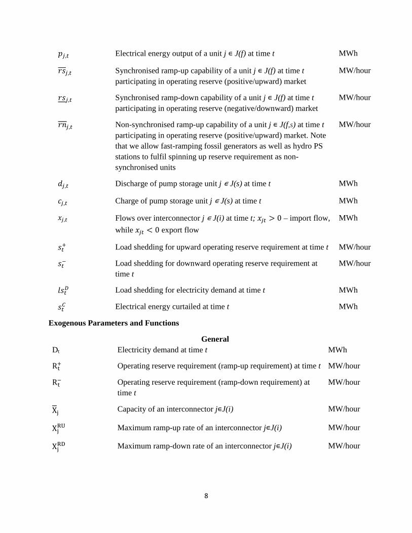
𝑝𝑝𝑗𝑗,𝑡𝑡 Electrical energy output of a unit j ∊ J(f) at time t MWh

𝑟𝑟𝑟𝑟𝑗𝑗,𝑡𝑡 Synchronised ramp-up capability of a unit j ∊ J(f) at time t participating in operating reserve (positive/upward) market

MW/hour

𝑟𝑟𝑟𝑟𝑗𝑗,𝑡𝑡 Synchronised ramp-down capability of a unit j ∊ J(f) at time t participating in operating reserve (negative/downward) market

MW/hour

𝑟𝑟𝑟𝑟𝑗𝑗,𝑡𝑡 Non-synchronised ramp-up capability of a unit j ∊ J(f,s) at time t participating in operating reserve (positive/upward) market. Note that we allow fast-ramping fossil generators as well as hydro PS stations to fulfil spinning up reserve requirement as non- synchronised units

MW/hour

𝑑𝑑𝑗𝑗,𝑡𝑡 Discharge of pump storage unit j ∊ J(s) at time t MWh

𝑐𝑐𝑗𝑗,𝑡𝑡 Charge of pump storage unit j ∊ J(s) at time t MWh

𝑥𝑥𝑗𝑗,𝑡𝑡 Flows over interconnector j ∊ J(i) at time t; 𝑥𝑥𝑗𝑗𝑡𝑡 > 0 – import flow, while 𝑥𝑥𝑗𝑗𝑡𝑡 < 0 export flow

MWh

𝑟𝑟𝑡𝑡+ Load shedding for upward operating reserve requirement at time t MW/hour

𝑟𝑟𝑡𝑡− Load shedding for downward operating reserve requirement at time t

MW/hour

𝑙𝑙𝑟𝑟𝑡𝑡𝐷𝐷 Load shedding for electricity demand at time t MWh

𝑟𝑟𝑡𝑡𝐶𝐶 Electrical energy curtailed at time t MWh

Exogenous Parameters and Functions

General Dt Electricity demand at time t MWh

Rt+

Operating reserve requirement (ramp-up requirement) at time t MW/hour

Rt−

Operating reserve requirement (ramp-down requirement) at time t

MW/hour

Xj Capacity of an interconnector j∊J(i) MW/hour

XjRU Maximum ramp-up rate of an interconnector j∊J(i) MW/hour

XjRD Maximum ramp-down rate of an interconnector j∊J(i) MW/hour

9

TL Transmission losses, % of gross supply injected into the transmission grid

n.a.

Thermal Generation HRj Heat rate of a generation unit j∊J(f) MWhth/MWhe

SUj Maximum ramp-up rate of a generation unit j∊J(f) during start up

MW/hour

SDj Maximum ramp-down rate of a generation unit j∊J(f) during shut down

MW/hour

RUj Maximum ramp-up rate of a generation unit j∊J(f) when committed

MW/hour

RDj Maximum ramp-down rate of a generation unit j∊J(f) when committed

MW/hour

Pj Minimum stable generation of a unit j∊J(f) MW/hour

Pȷ� Maximum power output of a unit j∊J(f) MW/hour

EJ Carbon intensity of a generator j∊J(f) tCO2/MWh

PLj Parasitic loss factor, % of maximum power output (𝑃𝑃𝚥𝚥�) %

Unit Commitment DTj Minimum down-time of a generation unit j∊J(f) hour

UTj Minimum up-time of a generation unit j∊J(f) hour

Lj Minimum down-time of a generation unit j∊J(f) at the start of the modelling horizon

hour

Gj Minimum up-time of a generation unit j∊J(f) at the start of the modelling horizon

hour

Hydro Pumped Storage

SEj Efficiency of charging a storage unit j ∊ J(s) %

Kj Maximum charge and discharge capacity of a storage unit j ∊ J(s)

MW/hour

SjINIT Initial energy stored at the beginning of a modelling horizon MWh

Sȷ� Maximum storage level MWh

10

Costs

Cj,tF Fuel cost of a generator j ∊ J(f) at time t £/MWhth

CtC Carbon cost £/tCO2

CjVAR Variable operating cost of a generator j∊J(f) and pump storage units j∊J(s)

£/MWhe

CjSU Cost of starting up a generator j∊J(f) £/start

CjSD Cost of shutting down a generator j∊J(f) £/shut

VD Value of loss load £/MWh

VR+ Cost of loss of spinning up reserve requirement £/MW/hour

VR− Cost of loss of spinning down reserve requirement £/MW/hour

CCL Cost of curtailing electrical energy output £/MWh

Pj,tIC Wholesale prices of external interconnected market j ∊ J(i) £/MWh

CR+ Payment for spinning up reserve availability £/MW/hour

3.2. Equations 3.2.1 Objective function

The objective of this optimization problem is to minimize total power system costs (eq. 1). The optimization assumes a central planner who has perfect information about the cost structure of all generation units, the levels of demand and all other technical conditions and as such assumes perfect foresight over the modelling horizon T when searching for optimal commitment statuses and economic dispatch of generation units while meeting a set of constraints (eq.2-24).

min�� � 𝑝𝑝𝑗𝑗,𝑡𝑡�Cj,tF HRj + CjVAR + EjCt𝐶𝐶�𝑗𝑗𝑗𝑗𝑗𝑗(𝑓𝑓)

+ � (𝑣𝑣𝑗𝑗,𝑡𝑡CjSU + 𝑤𝑤𝑗𝑗,𝑡𝑡CjSD)𝑗𝑗𝑗𝑗𝑗𝑗(𝑓𝑓)𝑡𝑡

+ � 𝑑𝑑𝑗𝑗,𝑡𝑡CjVAR

𝑗𝑗𝑗𝑗𝑗𝑗(𝑟𝑟)

+ � 𝑥𝑥𝑗𝑗,𝑡𝑡Pj,tIC

𝑗𝑗𝑗𝑗𝑗𝑗(𝑖𝑖)

+ CR+ � � (𝑟𝑟𝑟𝑟𝑗𝑗,𝑡𝑡 + 𝑟𝑟𝑟𝑟𝑗𝑗,𝑡𝑡)𝑗𝑗𝑗𝑗𝑗𝑗(𝑓𝑓,𝑟𝑟)

�

+ 𝑟𝑟𝑡𝑡+V𝑅𝑅+ + 𝑟𝑟𝑡𝑡_VR− + 𝑙𝑙𝑟𝑟𝑡𝑡𝐷𝐷𝑉𝑉D + 𝑟𝑟𝑡𝑡𝐶𝐶CCL�

(1)

11

3.2.2 System constraints First, electricity balance for every period t must be satisfied (eq. 2):

∀𝑡𝑡: � 𝑝𝑝𝑗𝑗,𝑡𝑡(1 − 𝑃𝑃𝑃𝑃𝑗𝑗)(1− 𝑇𝑇𝑃𝑃)𝑗𝑗∈𝑗𝑗(𝑓𝑓)

+ � 𝑑𝑑𝑗𝑗,𝑡𝑡(1 − 𝑇𝑇𝑃𝑃)𝑗𝑗∈𝑗𝑗(𝑠𝑠)

+ � 𝑥𝑥𝑗𝑗,𝑡𝑡𝑗𝑗∈𝑗𝑗(𝑖𝑖)

= (𝐷𝐷𝑡𝑡 − 𝑙𝑙𝑟𝑟𝑡𝑡𝐷𝐷 + 𝑟𝑟𝑡𝑡𝐶𝐶) + � 𝑐𝑐𝑗𝑗,𝑡𝑡𝑗𝑗∈𝑗𝑗(𝑠𝑠)

(2)

Equations 3 and 4 specify requirement for upward and downward operating reserve requirements for each period t. We allow both synchronised and non-synchronised units to participate in the upward spinning reserve market. Fast ramping stations like gas-fired units and hydro pumped storage can bid as non-synchronised units.

∀𝑡𝑡: � 𝑟𝑟𝑟𝑟𝑗𝑗,𝑡𝑡𝑗𝑗∈𝑗𝑗(𝑓𝑓)

+ � 𝑟𝑟𝑟𝑟𝑗𝑗,𝑡𝑡𝑗𝑗∈𝑗𝑗(𝑓𝑓,𝑠𝑠)

≥ 𝑅𝑅t+ − 𝑟𝑟𝑡𝑡+ (3)

∀𝑡𝑡: � 𝑟𝑟𝑟𝑟𝑗𝑗,𝑡𝑡𝑗𝑗∈𝑗𝑗(𝑓𝑓)

≥ Rt− − 𝑟𝑟𝑡𝑡− (4)

3.2.3. Thermal generation constraints The next two constraints relate to the capability of thermal generation units j ∊ J(f) to

ramp up (eq. 5) and down (eq. 6).

∀𝑗𝑗 ∈ 𝑗𝑗(𝑓𝑓), 𝑡𝑡: 𝑝𝑝𝑗𝑗,𝑡𝑡 + 𝑟𝑟𝑟𝑟𝑗𝑗,𝑡𝑡 − 𝑝𝑝𝑗𝑗,𝑡𝑡−1

≤ 𝑆𝑆𝑆𝑆𝑗𝑗�2 − 𝑢𝑢𝑗𝑗,𝑡𝑡 − 𝑢𝑢𝑗𝑗,𝑡𝑡−1� + 𝑅𝑅𝑆𝑆𝑗𝑗(1 + 𝑢𝑢𝑗𝑗,𝑡𝑡−1

− 𝑢𝑢𝑗𝑗,𝑡𝑡) (5)

∀𝑗𝑗 ∈ 𝑗𝑗(𝑓𝑓), 𝑡𝑡: 𝑝𝑝𝑗𝑗,𝑡𝑡−1 − 𝑝𝑝𝑗𝑗,𝑡𝑡 + 𝑟𝑟𝑟𝑟𝑗𝑗,𝑡𝑡

≤ 𝑆𝑆𝐷𝐷𝑗𝑗�2 − 𝑢𝑢𝑗𝑗,𝑡𝑡 − 𝑢𝑢𝑗𝑗,𝑡𝑡−1� + 𝑅𝑅𝐷𝐷𝑗𝑗(1 − 𝑢𝑢𝑗𝑗,𝑡𝑡−1

+ 𝑢𝑢𝑗𝑗,𝑡𝑡) (6)

Constraints 7 and 8 ensure that generating units are operated within their allowed range of outputs from its minimum generation level to its maximum allowed. Specifically, equation (7) specifies that every generating unit j ∊ J(f), if committed, should produce at least the minimum stable generating level accounting for the level of spinning down reserve committed in the reserve market, 𝑟𝑟𝑟𝑟𝑗𝑗,𝑡𝑡. Likewise, equation (8) ensures that power generated by a unit j ∊ J(f), if committed, should be less than the maximum power output given committed spinning up reserve, 𝑟𝑟𝑟𝑟𝑗𝑗,𝑡𝑡. Equation (9) ensures that non-synchronous units’ bids into the spinning up reserve do not exceed their starting ramp capability.

∀𝑗𝑗 ∈ 𝑗𝑗(𝑓𝑓), 𝑡𝑡: 𝑝𝑝𝑗𝑗,𝑡𝑡 ≥ 𝑢𝑢𝑗𝑗,𝑡𝑡𝑃𝑃𝑗𝑗 + 𝑟𝑟𝑟𝑟𝑗𝑗,𝑡𝑡 (7)

12

∀𝑗𝑗 ∈ 𝑗𝑗(𝑓𝑓), 𝑡𝑡: 𝑝𝑝𝑗𝑗,𝑡𝑡 ≤ 𝑢𝑢𝑗𝑗,𝑡𝑡𝑃𝑃𝚥𝚥� − 𝑟𝑟𝑟𝑟𝑗𝑗,𝑡𝑡 (8)

∀𝑗𝑗 ∈ 𝑗𝑗(𝑓𝑓), 𝑡𝑡: 𝑟𝑟𝑟𝑟𝑗𝑗,𝑡𝑡 ≤ (1 − 𝑢𝑢𝑗𝑗,𝑡𝑡)𝑆𝑆𝑆𝑆𝑗𝑗 (9)

3.2.4. Unit commitment constraints Logical constraint (10) ensures that start-up status, 𝑣𝑣𝑗𝑗,𝑡𝑡, and shut-down status, 𝑤𝑤𝑗𝑗,𝑡𝑡, take

an appropriate value (0, 1) when the units j ∊ J(f) starts up or shuts down.

∀𝑗𝑗 ∈ 𝑗𝑗(𝑓𝑓), 𝑡𝑡 𝑢𝑢𝑗𝑗,𝑡𝑡 − 𝑢𝑢𝑗𝑗,𝑡𝑡−1 = 𝑣𝑣𝑗𝑗,𝑡𝑡 − 𝑤𝑤𝑗𝑗,𝑡𝑡 (10)

Constraints (11-13) relate to minimum uptime requirements for fossil fuel generators. Equation (11) ensures that those units which were online before the modelling horizon starts, that is 𝐺𝐺𝑗𝑗 ≠ 0 , must stay online for the remaining minimum uptime (𝐺𝐺𝑗𝑗). Constraint (12) makes sure that if a unit is switched on it should stay online for at least UTj hours. Lastly, equation (13) ensure that if the remaining modelling hours are less than the minimum required uptime then the unit must stay online until the end of the modelling horizon, T, if it is committed.

∀𝑗𝑗 ∈ 𝑗𝑗(𝑓𝑓), 𝑡𝑡 ∈ �1;𝐺𝐺𝑗𝑗�,𝐺𝐺𝑗𝑗 ≠ 0 ∶ �(1 − 𝑢𝑢𝑗𝑗,𝑡𝑡)

𝐺𝐺𝑗𝑗

𝑡𝑡=1

= 0 (11)

∀𝑗𝑗 ∈ 𝑗𝑗(𝑓𝑓), 𝑡𝑡 ∈ �1 + 𝐺𝐺𝑗𝑗;𝑇𝑇 − 𝑆𝑆𝑇𝑇𝑗𝑗 + 1�: � 𝑢𝑢𝑗𝑗,𝑡𝑡𝑡𝑡

𝑡𝑡+𝑈𝑈𝑈𝑈𝑗𝑗−1

𝑡𝑡𝑡𝑡|𝑡𝑡𝑡𝑡≥𝑡𝑡

≥ 𝑆𝑆𝑇𝑇𝑗𝑗�𝑢𝑢𝑗𝑗,𝑡𝑡 − 𝑢𝑢𝑗𝑗,𝑡𝑡−1� (12)

∀𝑗𝑗 ∈ 𝑗𝑗(𝑓𝑓), 𝑡𝑡 ∈ �𝑇𝑇 − 𝑆𝑆𝑇𝑇𝑗𝑗 + 2;𝑇𝑇�: � �𝑢𝑢𝑗𝑗,𝑡𝑡𝑡𝑡 − [𝑢𝑢𝑗𝑗,𝑡𝑡 − 𝑢𝑢𝑗𝑗,𝑡𝑡−1]�𝑈𝑈

𝑡𝑡𝑡𝑡|𝑡𝑡𝑡𝑡≥𝑡𝑡

≥ 0 (13)

Following the same logic applied to the minimum uptime, equations (14-16) ensure feasibility of minimum downtime requirements for generating units. Thus, eq. (14) applies to those units that were offline before the start of the modelling horizon T and hence must stay offline for at least Lj hours. Equation (15) applies to those units that go offline between t=1 and T-DTj while the constraint (16) refers to units going offline after 𝑇𝑇 − 𝐷𝐷𝑇𝑇𝑗𝑗 + 2.

∀𝑗𝑗 ∈ 𝑗𝑗(𝑓𝑓), 𝑡𝑡 ∈ �1; 𝑃𝑃𝑗𝑗�,𝑃𝑃𝑗𝑗 ≠ 0 ∶ �𝑢𝑢𝑗𝑗,𝑡𝑡

𝐿𝐿𝑗𝑗

𝑡𝑡=1

= 0 (14)

∀𝑗𝑗 ∈ 𝑗𝑗(𝑓𝑓), 𝑡𝑡 ∈ �1 + 𝑃𝑃𝑗𝑗;𝑇𝑇 − 𝐷𝐷𝑇𝑇𝑗𝑗 + 1�: � 𝑢𝑢𝑗𝑗,𝑡𝑡𝑡𝑡

𝑡𝑡+𝑈𝑈𝑈𝑈𝑗𝑗−1

𝑡𝑡𝑡𝑡|𝑡𝑡𝑡𝑡≥𝑡𝑡

≥ 𝑆𝑆𝑇𝑇𝑗𝑗�𝑢𝑢𝑗𝑗,𝑡𝑡−1 − 𝑢𝑢𝑗𝑗,𝑡𝑡� (15)

13

∀𝑗𝑗 ∈ 𝑗𝑗(𝑓𝑓), 𝑡𝑡 ∈ �𝑇𝑇 − 𝐷𝐷𝑇𝑇𝑗𝑗 + 2;𝑇𝑇�: � �1 − 𝑢𝑢𝑗𝑗,𝑡𝑡𝑡𝑡 − [𝑢𝑢𝑗𝑗,𝑡𝑡−1 − 𝑢𝑢𝑗𝑗,𝑡𝑡]�𝑈𝑈

𝑡𝑡𝑡𝑡|𝑡𝑡𝑡𝑡≥𝑡𝑡

≥ 0 (16)

3.2.5. Energy Storage Constraints Hydro pump storage facilities are modelled using equations (17-20). Charging (eq. 17)

and discharging (eq. 18) cannot exceed capacity limitations while total energy volume stored cannot exceed storage volume capacity (eq. 19). Finally, eq. (20) makes sure that total energy discharging plus bids into the spinning up reserve market cannot exceed the energy volume that was stored before, 𝑆𝑆𝑗𝑗𝐼𝐼𝐼𝐼𝐼𝐼𝑈𝑈, and total net charging during the modelling horizon.

∀𝑗𝑗 ∈ 𝑗𝑗(𝑟𝑟), 𝑡𝑡: 𝑐𝑐𝑗𝑗,𝑡𝑡 ≤ 𝐾𝐾𝑗𝑗 (17)

∀𝑗𝑗 ∈ 𝑗𝑗(𝑟𝑟), 𝑡𝑡: 𝑑𝑑𝑗𝑗,𝑡𝑡 ≤ 𝐾𝐾𝑗𝑗 (18)

∀𝑗𝑗 ∈ 𝑗𝑗(𝑟𝑟), 𝑡𝑡: � (𝑆𝑆𝑆𝑆𝑗𝑗𝑐𝑐𝑗𝑗,𝑡𝑡𝑡𝑡 − 𝑑𝑑𝑗𝑗,𝑡𝑡𝑡𝑡)𝑡𝑡𝑡𝑡|𝑡𝑡𝑡𝑡≤𝑡𝑡

+ 𝑆𝑆𝑗𝑗𝐼𝐼𝐼𝐼𝐼𝐼𝑈𝑈 ≤ Sȷ� (19)

∀𝑗𝑗 ∈ 𝑗𝑗(𝑟𝑟), 𝑡𝑡: � (𝑑𝑑𝑗𝑗,𝑡𝑡𝑡𝑡 + 𝑟𝑟𝑟𝑟𝑗𝑗,𝑡𝑡𝑡𝑡+ − 𝑆𝑆𝑆𝑆𝑗𝑗𝑐𝑐𝑗𝑗,𝑡𝑡𝑡𝑡)

𝑡𝑡𝑡𝑡|𝑡𝑡𝑡𝑡≤𝑡𝑡

≤ 𝑆𝑆𝑗𝑗𝐼𝐼𝐼𝐼𝐼𝐼𝑈𝑈 (20)

3.2.6. Interconnector Flows Constraints Finally, import and export flows are restricted by available interconnection capacity (eq.

21 and 22). Note that ramp limits are sometime imposed on HVDC interconnector flows for system security reasons4, thus we allow these limits by introducing constraints (23) and (24).

∀𝑗𝑗 ∈ 𝑗𝑗(𝑖𝑖), 𝑡𝑡: 𝑥𝑥𝑗𝑗,𝑡𝑡 ≤ Xj (21)

∀𝑗𝑗 ∈ 𝑗𝑗(𝑖𝑖), 𝑡𝑡: 𝑥𝑥𝑗𝑗,𝑡𝑡 ≥ −Xj (22)

∀𝑗𝑗 ∈ 𝑗𝑗(𝑖𝑖), 𝑡𝑡: 𝑥𝑥𝑗𝑗,𝑡𝑡 − 𝑥𝑥𝑗𝑗,𝑡𝑡−1 ≤ XjRU (23)

∀𝑗𝑗 ∈ 𝑗𝑗(𝑖𝑖), 𝑡𝑡: 𝑥𝑥𝑗𝑗,𝑡𝑡−1 − 𝑥𝑥𝑗𝑗,𝑡𝑡 ≤ XjRD (24)

3.3. Optimization routines This section discusses optimization routines that were developed and implemented for

our modelling purposes.

3.3.1. Implementing a rolling horizon The application of the UC model to a real-world electricity system may result in a large

optimization problem, especially if it is to model every generation unit/plant, perhaps several 4 See Article 137(3) and (4) of the Commission Regulation (EU) 2017/1485 of 2 August 2017 establishing a guideline on electricity transmission system operation

14

hundred. Rolling horizon optimisation was implemented for our UC model to increase computational performance. A rolling horizon optimisation is one where the overall routine (for a full calendar year model) is reduced to a specified number of sub-problems to avoid excessive solve times or memory issues with the machine used for the optimisation. It assumes that if optimality is achieved in individual simulation runs which form part of a larger model, then overall optimality is achieved for the complete solve window. As a practical matter, the degree of uncertainty about future demand, renewables output and plant availability limit the time horizon over which operational systems optimize.

The approach for transitioning between two modelling periods (e.g., T1 to T2) is to take a snapshot of the system at a time prior to the point of transition: t2 = T1 −q1, where T1 is equal to K, the number of time intervals within each horizon roll, and q1 is the selected cut-off time (see Figure 1).

Figure 1: Implementing Rolling Horizon optimization

This snapshot is logged with the dispatch status and generation levels of the various generators. It is also crucial that the energy storage level of storage systems is also recorded. The next optimisation window is then solved from t2 to T2 = K. Note that s1=s2=…=sm=s and q1=q2=…=qm=q, where m is number of rolling horizons that will be required to cover the annual modelling horizon (e.g. one year or 8760 hours). Clearly m depends on s and q. For example, if K=100 hours and q=30 hours, hence s=70 hours then m=8760/70=126 rolling horizons that need to be modelled and solved; that is, there will be 126 rolling horizons with 70 hours each and the last 127th horizon will have only 60 hours. However, since q=30 hours, every next rolling horizon the model ‘resolves’ the previous 30 hours of the preceding horizon. This creates ‘redundancy’ but this is needed to ensure that solution of each horizon is optimal and would be as close to solving the entire 8760 hours in one go as possible. In this sense, the larger is the q the closer to full optimality the combined results of each horizon would be. Sensitivity analysis regarding setting the parameter K will reveal the trade-off between total solution time needed to solve 8760 hours vs. differences in results due to different values of K.

T1

T2

Tm

q1

q2

qm

s1 t1

t2 s2

tm sm

………

15

The inputs to the second simulation (T2) are the commitment and output status of every plant and the energy storage levels. This preserves the state of the system while the demand profile and other exogenous inputs for the new horizon are added. This process is repeated until the full modelling horizon (e.g., one year or 8760 hours) is satisfied.

4. Application: A GB Unit Commitment and Economic Dispatch Model 4.1. Motivation

The UK along with many other nations is focussed on delivering significant decarbonisation in the power sector as part of emissions reduction efforts (CCC, 2018). Forecasts suggest that to meet the economy-wide emissions reduction targets set for 2030, the UK must reduce the emissions intensity of the power sector to approximately 100 gCO2/kWh. To reach this target will require high levels of renewable generation. In 2017, renewable5 electricity provided 29% of the total annual supply, while the expected levels of renewable generation in 2030 are required to increase to between 48-73%6 of total supply depending on scenarios (CCC, 2018). While a high renewables scenario satisfies one leg of the UK’s ‘energy trilemma’ (WEC, 2016), electricity markets also need to provide energy supply at least-cost and ensure reliability of supply.

Reliable operation of a power system is defined by the National Renewable Energy Council as one continuing to operate "within equipment and electric system thermal, voltage, and stability limits so that instability, uncontrolled separation, or cascading failures of such system will not occur as a result of a sudden disturbance, including a cybersecurity incident, or unanticipated failure of system elements" (NERC, 2017). Ensuring reliability of supply in these high renewables scenarios can be challenging when considering the intermittency and seasonal variability of solar and wind. If renewable energy output is low then the power system must be able to replace it with alternative supply from flexible generation, demand reduction, imports or storage.

The UK energy regulator, OFGEM, defines a flexible source as one that has "the ability to ramp generation or demand up or down quickly in response to changing market conditions" (Ofgem, 2015). Some examples of such sources include (but are not limited to) gas-fired power (both closed-cycle and open-cycle gas turbines, CCGT, OCGT), diesel or gas-fired reciprocating engines, pumped and battery storage and interconnectors, as well as demand response (not modelled here). These should be available in sufficient volumes to respond to the sudden and

5 This includes natural flow hydro, wind, wave and solar photovoltaics as well as thermal renewables (biomass and non-biomass, e.g., biogas and other ‘renewable’ gases). See Digest of UK Energy Statistics (DUKES table 5.6) at: https://assets.publishing.service.gov.uk/government/uploads/system/uploads/attachment_data/file/729385/DUKES_5.6.xls (accessed March 2019). 6 Figure 2.7. in CCC (2018) report. We deem the following sources as ‘renewables’ using CCC scenarios: Onshore wind, Offshore wind, Solar, Tidal, Biomass, Hydro. See accompanied excel file with projections available at: https://www.theccc.org.uk/wp-content/uploads/2018/06/02-Exhibits-Power-PR18.xlsx (accessed March 2019)

16

also persistent swings for a sufficiently high proportion of the time to maintain the specified reliability, such as controlled demand reductions not more than three hours per year on average.

A desirable market design of a future electricity system with high level of renewables is one that meets the targeted emissions reduction, provides the security of supply needed and is delivered at least cost to consumers.

Many energy models have been developed and calibrated for the UK (surveyed in Hall et al., 2016 and in §2.2). While these models have been widely used, there are fewer models of the GB electricity system specifically (also discussed in §2.2). Given that, the primary objective of this paper was to formulate a UC model (see §3) and apply it to the GB electricity market. A secondary objective was to report, document and assess the data sources used for calibrating the model. The model is calibrated to 2015, and subjected to a sensitivity analysis to test the robustness of the model and the data quality. The rest of this section reports on data input and assumptions, calibration and sensitivity analysis. 4.2. Data input and assumptions

A full account of sources of data input and assumptions is given in Appendix 1. This section discusses the main assumptions used to calibrate the model.

4.2.1. Generation technologies modelled Wind and solar generation have effectively zero marginal cost and so will always be

dispatched first.7 Nuclear generation has a relatively low marginal cost so can be modelled exogenously. Biomass generation, like wind and solar, receives government renewables support (e.g., in the form of either ROCs or CfDs) and so they can also be modelled exogenously. Interconnectors are modelled ‘semi-endogenously’ in that we treat interconnectors as:

1. generators, taking their historical wholesale day-ahead prices from the market coupling algorithm as their marginal costs. Hence, interconnectors are part of GB’s merit order. or

2. loads, whenever their historical wholesale prices are higher than GB’s system marginal cost and GB generators have spare capacity to supply those loads.

The current version of the model solves the dispatch and unit commitment problem for coal- and gas-fired generation plants as well as hydro pump storage operations (pumping and discharging) and interconnector flows to meet the defined residual demand (eq. 2 and Appendix 1, Section A.2).

4.2.2. Time horizon and granularity We simulate the GB electricity market at hourly granularity. The simulation time horizon

is one year (8760 hours). The initial period was set to be one month prior to the modelling horizon; also, in order to minimise ‘the end’ of model horizon issues we set the model to run for one additional month after the model horizon. Thus, for the year 2015, the initial time period is the 1st hour of the 1st of December 2014 while the last time period of the modelling is the last 7 Wind has a non-negligible variable cost that is less than the subsidy, so its perceived cost is low (actually negative).

17

hour of the 31st of January 2016. The model therefore runs for two additional months (14 months in total) such that we have ‘optimal’ starting and end points for each plant and hydro pumped storage levels.

In addition, we assume that at the initial period all pumped storage (PS) stations are full – that is, in total, 23.9 GWh of electricity is available at the beginning of the modelling horizon (see Appendix 1, Section A.5). This assumption is not critical as the model runs for an additional month before the actual model timeframe so that the optimal storage level by the 1st hour of January 1, 2015 will be determined by the model.

4.3. Calibration We chose to calibrate the model to 2015 as that was the latest comprehensive dataset of

existing power plants (details in Appendix 1, Section A.6) reported by National Grid in its 2015 Electricity Ten Year Statement (National Grid, 2015). That report also maps the plants to GB transmission zones and boundaries (where physical network constraints are likely to occur) as well as providing forecasts of plant additions and retirements from 2015-2035. The calibration for 2015 is consistent with this power plant dataset. We use the actual annual generation mix of 2015 as a benchmark against which we report all our modelling and calibration results.

A number of factors could influence dispatch decisions and hence the resulting generation mix:

1. Fuel and interconnector prices, carbon and variable operating and maintenance costs (var. opex) faced by a generating unit

2. Generator’s cycling cost (start-up and shut-down costs) 3. Generator’s thermal efficiency and carbon intensity 4. Generator’s net vs gross output (parasitic loss factor) and its outage/capacity factor 5. operating reserve requirements, gross capacity of a unit and its ramping capability.

These techno-economic factors are the main ones which will determine the commitment status and dispatch order of plants. Some of these parameters are well defined (each unit’s generation capacity, fuel prices and carbon cost). Others are subject to numerous uncertainties (e.g., cycling costs, variable opex, thermal efficiency and hence carbon intensity). Some involve simplifications (e.g., operating reserve requirements, outage/capacity factors, parasitic loss factors). Details of data sources and assumptions are given in Appendix 1 and other sections of this paper. The calibration process involves ensuring that the dispatch delivers the fuel mix observed (at least on average) and for that we only adjust two parameters: (i) the cost function of a generator, and (ii) and wholesale prices of interconnected markets.

To manipulate the cost functions of a generator we use multiplicative fuel mix calibration parameters, Mj, as follows:

𝐶𝐶𝑗𝑗,𝑡𝑡 = �𝑀𝑀𝑗𝑗𝐶𝐶𝑗𝑗,𝑡𝑡𝐹𝐹 𝐻𝐻𝑅𝑅𝑗𝑗 + 𝐶𝐶𝑗𝑗𝑉𝑉𝑉𝑉𝑅𝑅 + 𝑆𝑆𝑗𝑗𝐶𝐶𝑡𝑡𝐶𝐶� (25)

18

For tractability and simplicity, this calibration parameter is changed either to all coal or all gas units and not individual plants, j. We change the historical hourly prices for interconnected markets by applying a similar multiplicative parameter for the whole year such that, on average, annual net interconnection flows match historically observed flows.

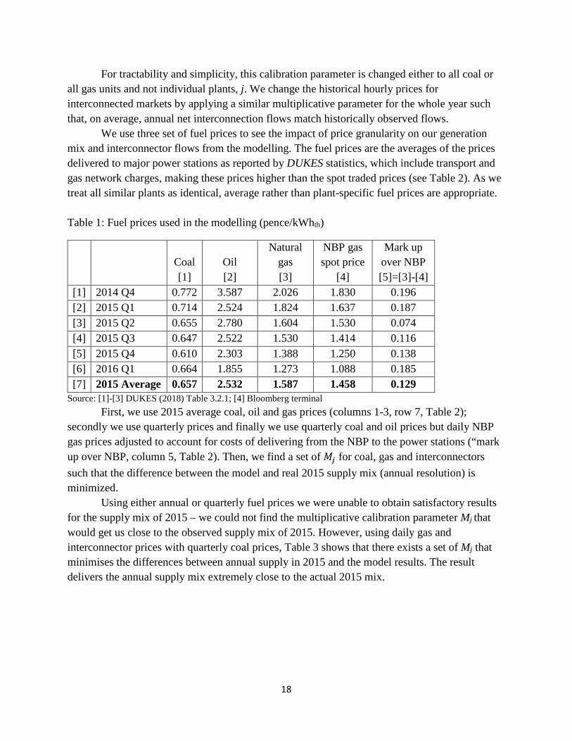
We use three set of fuel prices to see the impact of price granularity on our generation mix and interconnector flows from the modelling. The fuel prices are the averages of the prices delivered to major power stations as reported by DUKES statistics, which include transport and gas network charges, making these prices higher than the spot traded prices (see Table 2). As we treat all similar plants as identical, average rather than plant-specific fuel prices are appropriate.

Table 1: Fuel prices used in the modelling (pence/kWhth)

Coal [1]

Oil [2]

Natural gas [3]

NBP gas spot price

[4]

Mark up over NBP [5]=[3]-[4]

[1] 2014 Q4 0.772 3.587 2.026 1.830 0.196 [2] 2015 Q1 0.714 2.524 1.824 1.637 0.187 [3] 2015 Q2 0.655 2.780 1.604 1.530 0.074 [4] 2015 Q3 0.647 2.522 1.530 1.414 0.116 [5] 2015 Q4 0.610 2.303 1.388 1.250 0.138 [6] 2016 Q1 0.664 1.855 1.273 1.088 0.185 [7] 2015 Average 0.657 2.532 1.587 1.458 0.129

Source: [1]-[3] DUKES (2018) Table 3.2.1; [4] Bloomberg terminal First, we use 2015 average coal, oil and gas prices (columns 1-3, row 7, Table 2);

secondly we use quarterly prices and finally we use quarterly coal and oil prices but daily NBP gas prices adjusted to account for costs of delivering from the NBP to the power stations (“mark up over NBP, column 5, Table 2). Then, we find a set of 𝑀𝑀𝑗𝑗 for coal, gas and interconnectors such that the difference between the model and real 2015 supply mix (annual resolution) is minimized.

Using either annual or quarterly fuel prices we were unable to obtain satisfactory results for the supply mix of 2015 – we could not find the multiplicative calibration parameter Mj that would get us close to the observed supply mix of 2015. However, using daily gas and interconnector prices with quarterly coal prices, Table 3 shows that there exists a set of Mj that minimises the differences between annual supply in 2015 and the model results. The result delivers the annual supply mix extremely close to the actual 2015 mix.

19

Table 2: Calibration results for the year 2015 using daily gas prices and quarterly coal prices

Annual supply, TWh Supply mix calibration

parameter, 𝐌𝐌𝐣𝐣 2015 [1]

Simulation [2]

Delta [3]=[2]-[1]

Interconnectors

Britned (GB-NL) 8.00 7.93 -0.07 0.750 EWIC (GB-IE) -1.07 -1.10 -0.03 1.090 IFA (GB-FR) 13.85 13.92 0.07 0.800 Moyle (GB-NI) -0.19 -0.27 -0.08 1.090

Fossil fuel generation

Coal 74.49 74.55 0.06 1.014 Gas 84.39 84.52 0.13 1.044

Hydro pumped storage

Discharge 2.67 1.75 -0.92 n.a. Charge -3.57 -2.57 0.99 n.a.

The differences between the modelling results and the observed data is within 3% except for interconnector flows through Moyle and pumped storage stations. The absolute difference for flows over Moyle is relatively small but large in relative terms (42% over actual flows). We could further calibrate the flows for EWIC and Moyle by applying different calibration parameters but deemed the results in Table 3 very satisfactory for our purposes. In 2015 neither EWIC nor Moyle were coupled to GB (IFA and BritNed were) and only managed to flow electricity in the right direction less than 60% of the time (SEM, 2017).

Differences in hydro PS reflect the fact that in the model the PS results are driven only by price arbitrage opportunities whereas in reality PS stations fulfil a number of balancing and ancillary services that are not captured in the current model. Further, Cruachan PS station has access to a catchment area and so enjoys natural inflows that might offer “free” storage. It is reported that 10% of annual electricity output from the Cruachan PS station is produced using rain and to that extent operates as a conventional run-of-river hydropower station (Scottish Power, 2011).

Finally, we compared the calibrated system marginal prices (SMP) with the 2015 GB day-ahead prices and found that, on average, our SMPs are 7.6% higher than the 2015 actual day-ahead prices. This is a result of ‘marking up’ fuel (gas by 4.4% and coal by 1.4%) and interconnector prices to achieve the 2015 supply mix (see Table 3). Therefore, we adjust the entire supply curve down by 7.6% and re-run the model to achieve the best possible fit in terms of annual supply mix (Table 3) and SMPs (Figure 2).

Applying these multiplicative fuel mix calibration parameters addresses the systematic biases in the quality of input data, such as fuel prices which are very heterogenous (specific to each plant and location), as well as systematic biases inherent to the modelling approach, such as determinism and perfect foresight. Using these multiplicative correction biases parameters for sensitivity and further scenario-based analysis appears defensible and more plausible than application of specific hourly mark-up parameter which is calibrated to historical data to get a very close match between model output and real data. In this regard, using this multiplicative

20

correction biases parameter for sensitivity and further scenario-based analysis is more plausible than, for example, hourly mark-up parameters calibrated to historical data.

Figure 2: GB load duration curves (LDC) – 2015 vs simulated results

4.4. Sensitivity analysis This section reports the sensitivity to structural features of the model. We take the

calibrated baseline from §4.3 as the reference point and change the model structure along three key dimensions:

1. The length of the rolling modelling horizon, 2. The size of operating reserve requirements, 3. Binary and commitment decisions, plant flexibility parameters and simple economic

dispatch solution without binary decisions.

4.4.1. Impact of modelling horizon length on results and solution time The baseline sets the rolling horizon at 100 hours, that is, K=100. The cut-off time is 30%

of this, i.e., 30 hours (see §3.3.1). One very important implication is that due to hydro PS constraints (eq. 19 and 20) the longer is K the less the problem is ‘compact’ – the size of the model due to the summing over ‘t’ becomes huge. Table 4 shows this has a dramatic impact on the solution time without any meaningful improvement in the ‘quality’ of the results.

One can see that increasing the number of hours from 100 hours (baseline) to 720 hours (K720) increases the total solution time by a factor of five. However, the impact on the results is only a slight improvement in PS dispatch (i.e., an increase in PS utilization). This confirms our initial expectation that the number of hours in each horizon will most likely influence dispatch of units with intertemporal constraints such as eq. (19-20) for PS and conventional generation constraints related to minimum up and down time (eq. 11-16). It is interesting that the higher PS utilization is associated with higher outputs from gas plants, probably because gas prices varies

21

daily and hence PS can realize daily arbitrage opportunities more efficiently compared to coal quarterly prices.

There is some non-linearity in the relationship between the number of hours and PS utilization – K180 seems to produce the highest PS utilization while in K48 we see the lowest PS utilization. Again, this might be due to fuel price dynamics (gas prices in particular) in that a moving 180-hour optimization window might capture most of gas price volatility and hence higher PS utilization rather than a moving 720-hour window.

Table 3: Impact of modelling horizon length on results

Annual supply, TWh 2015 BASE K720 K360 K180 K48 Coal 74.49 74.55 73.31 73.32 73.13 77.19 Gas 84.39 84.52 85.98 85.95 86.26 81.25 Hydro PS discharge 2.67 1.75 1.78 1.79 1.84 1.67 Hydro PS charge -3.57 -2.57 -2.63 -2.64 -2.70 -2.46 Total interconnector flows 20.60 20.48 20.28 20.31 20.20 21.06

Britned flows 8.00 7.93 7.93 7.93 7.87 8.04 EWIC flows -1.07 -1.10 -1.12 -1.12 -1.13 -0.98 IFA flows 13.85 13.92 13.78 13.79 13.77 14.22 Moyle flows -0.19 -0.27 -0.30 -0.29 -0.30 -0.21

System marginal price, £/MWh

Mean 40.43 39.01 38.74 38.80 38.76 39.56 Min 3.99 8.13 8.13 8.13 8.13 8.07 Max 167.91 187.21 193.76 194.42 195.62 186.56

Mathematical program characteristics

solve time, seconds 1,051 4,943 2,270 1,393 774 Number of constraints 39,401 283,681 141,841 70,921 18,913 Number of variables (total) 34,301 246,961 123,481 61,741 16,465

of which integer variables 14,400 103,680 51,840 25,920 6,912 N non-zeros 287,120 6,537,340 1,972,180 661,600 112,348 ratio integer/non-integer variables 0.72 0.72 0.72 0.72 0.72

Note: solve time is reported for the entire modelling horizon of 14 months or 10248 hours.

All in all, one can see that a rather drastic change in the length of one modelling horizon from 48 hours to 720 hours produces results which are very similar. At least for this unit commitment model of the GB electricity market the model time horizon should be 48-180 hours to reduce the solution time. As already noted, uncertainty about future demand, renewables

22

output and plant availability limit the time horizon over which operational systems optimize so optimizing beyond a couple of days may not make much sense.

In general, the solution time increases linearly with the size of the optimization problem (Figure 3). However, the number of non-zeros (data that the model needs to process) slightly better explains the solution time than the number of constraints and variables. This highlights the importance of model’s compactness and the influence of this has on the solution time. For example, comparing model characteristics for the baseline and K720 shows that while the number of constraints and variables increases by a factor of 7.2, the number non-zeros increases by a factor of 22.8; and this increases the solution time by a factor of 4.7.

Figure 3: Solution time and the size of the unit commitment problem

The length of time horizon should be guided by the minimum up/down times as well as the total storage volume, as these parameters influence the optimality of each modelling horizon. For example, if coal stations have a minimum up (and down) time of 24 hours then it would be desirable to model at least 25 hours in one modelling horizon to ensure the model can decide on their commitment status. Similarly, if all PS stations can store up to 24 hours’ worth of energy then the modelling horizon should be at least twice 24 hours to account for one cycle of charge and discharge. This will ensure that we are not constraining the model and the search space when it comes to PS dispatch decisions.

The baseline and all the sensitivities were modelled on a 64-bit Windows 7 PC with 32 GB of RAM and 2 multi-core Intel Xeon CPU E5-2650 2.6 GHz processors (16 cores in total).8 The baseline has also been modelled on two other machines with different specifications to see how sensitive the solution time is to the spec of the PC:

8 2.6 GHz base frequency and 3.4 GHz max turbo frequency

23

1. 64-bit Windows 10 PC with 8 GB of RAM and one multi-core (4 cores in total) i5-4590 with 3.3 GHz processor;9

2. 64-bit Windows 10 Laptop with 16 GB of RAM and one multi-core (4 cores in total) i7-4702HQ with 2.20 GHz processor.10

We use AIMMS11 as the modelling environment and CPLEX solver version 12.7.1 with the MIP absolute optimality tolerance of 1e-6 and the relative optimality tolerance of 0.01. Rather surprisingly the solution time for the baseline on the i5-4590 machine was 593 seconds, almost twice as fast as the 2 multi-core processors machine. On a laptop, the solution time as significantly slower – 10,665 seconds. Clearly CPU clock speed significantly influences the solution time rather than the number of cores. This is principally because our model calibrated to the 2015 GB electricity market has a relatively small branch and bound tree and hence the number of cores does not matter too much.

4.4.2. Operating reserve and fast-ramping generation units Dimensioning (sizing) operating reserve requirements is important in that it could greatly

influence the dispatch order. For example, spin-up reserve requirement (eq. 3) will make sure that a certain amount of reserve capacity will be taken ‘off’ the dispatch order (supply curve). Traditionally, the spin-up reserve is equal to the capacity of the largest generation (or interconnector) plus a percentage of demand to reflect possible errors in demand forecasting. But with the rapid uptake of VRE, the spin-up requirement also needs to consider forecast errors of the VRE resources (wind and solar). This means that operating reserves will become increasingly volatile. The volatility will be dependent on VRE capacity but also how much assurance a system operator wants to have to hedge against forecasts errors. For example, the assurance will involve a decision whether to hedge against 99% of possible swings in demand and VRE generation forecast errors (three standard deviations of forecast errors) or less (more) (see Appendix 1, A.3 for further discussions on this point). This section examines the impact of (i) sizing of the operating reserve, and (ii) types of units who can fulfil reserve requirements on modelling results.

In the baseline we define spinning up requirement as the sum of the capacity of the largest generator plus three standard deviations (SD, σ) of demand and wind forecast errors (see eq. A.6 in Appendix 1). Three SDs will cover 99% of the distribution of errors while four SDs will cover 99.99% while two SDs will cover 95%. Taking a zero SD means not considering errors in demand and VRE resource forecasts. The operating reserve is then static over the entire modelling horizon and equal to the capacity of the largest generating unit connected to the system. We also model a case without operating reserve (“no reserve” case) equations (3 and 4).

In eq. (3) both synchronized and non-synchronized units can bid into the spinning up reserve market. Non-synchronized units are fast ramping generators that can spin up very quickly

9 3.3 GHz base frequency and 3.7 GHz max turbo frequency 10 2.2 GHz base frequency and 3.2 GHz max turbo frequency 11 https://aimms.com/

24

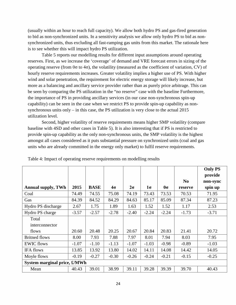
(usually within an hour to reach full capacity). We allow both hydro PS and gas-fired generation to bid as non-synchronized units. In a sensitivity analysis we allow only hydro PS to bid as non-synchronized units, thus excluding all fast-ramping gas units from this market. The rationale here is to see whether this will impact hydro PS utilization.

Table 5 reports our modelling results for different input assumptions around operating reserves. First, as we increase the ‘coverage’ of demand and VRE forecast errors in sizing of the operating reserve (from 0σ to 4σ), the volatility (measured as the coefficient of variation, CV) of hourly reserve requirements increases. Greater volatility implies a higher use of PS. With higher wind and solar penetration, the requirement for electric energy storage will likely increase, but more as a balancing and ancillary service provider rather than as purely price arbitrage. This can be seen by comparing the PS utilization in the “no reserve” case with the baseline Furthermore, the importance of PS in providing ancillary services (in our case non-synchronous spin-up capability) can be seen in the case when we restrict PS to provide spin-up capability as non-synchronous units only – in this case, the PS utilization is very close to the actual 2015 utilization level.

Second, higher volatility of reserve requirements means higher SMP volatility (compare baseline with 4SD and other cases in Table 5). It is also interesting that if PS is restricted to provide spin-up capability as the only non-synchronous units, the SMP volatility is the highest amongst all cases considered as it puts substantial pressure on synchronized units (coal and gas units who are already committed in the energy only market) to fulfil reserve requirements.

Table 4: Impact of operating reserve requirements on modelling results

Annual supply, TWh 2015 BASE 4σ 2σ 1σ 0σ No

reserve

Only PS provide

non-sync spin up

Coal 74.49 74.55 75.08 74.19 73.43 73.53 70.53 71.95 Gas 84.39 84.52 84.29 84.63 85.17 85.09 87.34 87.23 Hydro PS discharge 2.67 1.75 1.89 1.63 1.52 1.52 1.17 2.53 Hydro PS charge -3.57 -2.57 -2.78 -2.40 -2.24 -2.24 -1.73 -3.71

Total interconnector flows 20.60 20.48 20.25 20.67 20.84 20.83 21.41 20.72

Britned flows 8.00 7.93 7.88 7.97 8.01 7.94 8.03 7.95 EWIC flows -1.07 -1.10 -1.13 -1.07 -1.03 -0.98 -0.89 -1.03 IFA flows 13.85 13.92 13.80 14.02 14.11 14.08 14.42 14.05 Moyle flows -0.19 -0.27 -0.30 -0.26 -0.24 -0.21 -0.15 -0.25 System marginal price, £/MWh

Mean 40.43 39.01 38.99 39.11 39.28 39.39 39.70 40.43

25

Min 3.99 8.13 8.13 8.13 8.16 8.13 6.65 6.65 Max 167.91 187.21 195.78 188.05 185.01 172.78 148.34 142.20 CV 26% 28% 30% 27% 26% 26% 23% 37%

Spin up requirement (MW/hour) Mean

4564 5331 3796 3028 2260 0 4564 Min 3733 4224 3242 2751 2260 0 3733 Max 5658 6791 4525 3393 2260 0 5658 CV 15% 17% 12% 7% 0% 0 0

Spin down requirement (MW/hour) Mean

2282 2666 1898 1514 1130 0 2282 Min 1867 2112 1621 1376 1130 0 1867 Max 2829 3395 2263 1696 1130 0 2829 CV 15% 17% 12% 7% 0% 0 0

Note: CV – coefficient variation is determined as a ratio of standard deviation to the mean; 4σ means four standard deviations (SD) of demand and wind forecast errors; 3σ – three SD and so on.

Third, in all our cases, non-synchronized gas-fired capacity will cover 99% of all spin-up reserve requirements (Table 6). It is only when we exclude non-synchronized gas-fired capacity from providing spin-up reserves is the spin up reserve market roughly equally divided between online coal and gas units as well as PS units.

All in all, defining operating reserve requirements is important as it will influence dispatch order and SMP. That said, our sensitivity analysis shows that the variations in annual output of gas and coal is of order of 4% and 7% respectively and 80% for PS. Clearly the impact on the PS utilization is the greatest.

Table 5: Provision of reserves by technology type, MW/hour (as % of hourly average reserve requirement)

BASE 4σ 2σ 1σ 0σ

Only PS provide non-sync spin up

Spin

up

rese

rve synchronised coal

1 (0.0%)

1 (0.0%)

0 (0.0%)

0 (0.0%)

0 (0.0%)

2,139 (46.9%)

synchronised gas 5

(0.1%) 14

(0.3%) 3

(0.1%) 0

(0.0%) 0

(0.0%) 2,414

(52.9%)

Non-synchronised gas 4,557

(99.9%) 5,313

(99.7%) 3,793

(99.9%) 3,028

(100.0%) 2,260

(100.0%) 0

(0.0%)

Non-synchronised PS 1

(0.0%) 2

(0.0%) 0

(0.0%) 0

(0.0%) 0

(0.0%) 8

(0.2%)

Spin

do

wn

synchronised coal 843

(35.7%) 1,015

(37.1%) 664

(33.4%) 448

(27.9%) 243

(19.8%) 738

(31.4%)

26

synchronised gas 1,518

(64.3%) 1,724

(62.9%) 1,321

(66.6%) 1,157

(72.1%) 983

(80.2%) 1,615

(68.6%) Note: for each scenario, summing up all bids for spin (down) up reserve should be equal to average hourly spin up (down) reserve requirement reported in Table 5.

4.4.3. Plant flexibility and commitment This section addresses a question of power system flexibility and what it means for

dispatch and SMP. To this end, we run several sensitivities around the unit commitment parameters such as:

1. Ramping limits and on/off commitment time 2. Exclusion of binaries variables dealing with start-up and shut down and commitment

status of dispatchable generation from the optimization problem

We define two sensitivities around the cycling characteristics for gas- and coal-fired power stations to represent a potentially ‘highly’ flexible power system and a highly ‘inflexible’ one. Baseline assumptions for cycling parameters are in Appendix 1, Table A. 4. For a flexible (inflexible) system we increase (reduce) ramping rates and reduce (increase) the minimum up/down time by a factor of two from the baseline cycling parameters. Under the inflexible power system sensitivity we might see load shedding and power curtailment to deal with inflexibility imposed on generation units.

For the third sensitivity we exclude all binary variables (commitment status, start-up and shut-down variables) so the optimization problem is reduced to a simple linear program (LP) with the following set of equations: 1-4 (objective function and system constraints), 5-8 (thermal ramping limits), 17-20 (bulk storage), 21-24 (interconnector flows). Minimum generation term (𝑢𝑢𝑗𝑗,𝑡𝑡𝑃𝑃𝑗𝑗) are removed from the eq. (7) as commitment status was removed from this sensitivity

analysis. This LP might represent a very flexible thermal power system and hence the results could be similar to those from a unit commitment model with highly flexible cycling parameters. As before, we benchmark the results from these sensitivities (Table 7) with the ones obtained for the baseline case.

Table 6: Impact of thermal generation flexibility on modelling results

Annual supply, TWh 2015 BASE Flexible Inflexible LP Coal 74.49 74.55 43.80 58.08 42.99 Gas 84.39 84.52 112.83 113.45 111.60 Hydro PS discharge 2.67 1.75 1.42 3.38 0.09 Hydro PS charge 3.57 -2.57 -2.08 -4.94 -0.14 Total interconnector flows 20.60 20.48 22.75 8.98 24.18

Britned 8.00 7.93 8.27 4.53 8.31 EWIC -1.07 -1.10 -0.51 -2.28 -0.07 IFA 13.85 13.92 14.95 7.67 15.64

27

Moyle -0.19 -0.27 0.03 -0.95 0.30 System marginal price, £/MWh

Mean 40.43 39.01 41.21 31.80 42.35 Min 3.99 8.13 8.17 -47.22 21.84 Max 167.91 187.21 212.87 133.07 142.22 CV 26% 28% 27% 52% 15%

Annual system operating cost, £ mn, of which:

n.a.

7,393 7,297 7,874 7,193 Fuel cost 6,563 6,391 7,324 6,297 Start and shut down cost 20 27 0 n.a.* Spinning reserve cost 306 306 306 306 PS variable O&M cost 17 14 33 0.92 Net import cost 487 559 190 589 Load shedding cost 0 0 0 0 Cost of loss of operating reserve 0.46 0.14 21.00 1.17 Wind curtailment cost 0 0 10 0

Note: * in the LP we do not model binary decisions and unit commitment constraints so start up and shut down cost is not relevant in this case

Cycling characteristics can change the supply mix quite significantly. In both cases (flexible and inflexible) we see a clear shift to a gas-dominant supply mix with some marginal variations around how much coal generates from one sensitivity to another one. Thus, in the inflexible case, coal generates about 32% more on an annual basis than it would generate under the flexible case but 22% less than under the baseline.

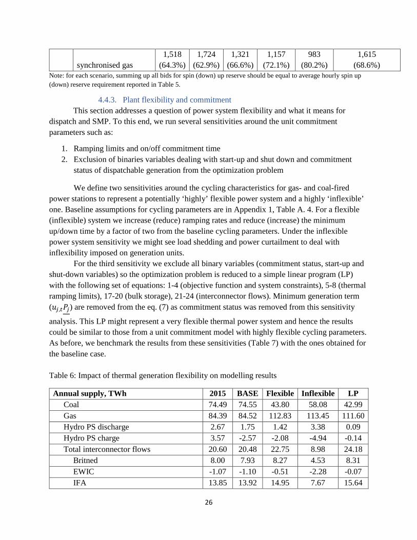
The reason is that when coal is more flexible it responds to fuel price dynamics more compared to the situation when coal is less flexible (baseline or inflexible cases). This is evident by looking at hourly coal generation for the three cases (Figure 4). In summer months when coal is flexible it ramps up and down quite often (start-up and shut-down cost is £27 million vs £20 m. in the baseline). When it is inflexible (red line) coal generates at minimum stable generation level and rarely cycles (start-up and shut-down costs are zero). In the baseline coal is more flexible and ramps up and down to the minimum stable generation. Because the minimum up and down time has been reduced dramatically for coal (and gas) under the flexible case, coal units do a lot of cycling (starts and shuts).

28

Figure 4: Coal generation under the baseline and two flexibility cases

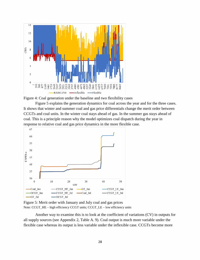
Figure 5 explains the generation dynamics for coal across the year and for the three cases. It shows that winter and summer coal and gas price differentials change the merit order between CCGTs and coal units. In the winter coal stays ahead of gas. In the summer gas stays ahead of coal. This is a principle reason why the model optimizes coal dispatch during the year in response to relative coal and gas price dynamics in the more flexible case.

Figure 5: Merit order with January and July coal and gas prices Note: CCGT_HE – high efficiency CCGT units; CCGT_LE – low efficiency units

Another way to examine this is to look at the coefficient of variations (CV) in outputs for all supply sources (see Appendix 2, Table A. 9). Coal output is much more variable under the flexible case whereas its output is less variable under the inflexible case. CCGTs become more

29

baseload when flexible and ramp more in the baseline (but for some CCGTs, the magnitude of ramps is wider under the flexible vs. baseline cases).

In the inflexible case, most CCGTs are baseload and PS utilization is very high, but variations in charge/discharge are lower than in the baseline or flexible case (see Appendix 2, Table A. 9). This suggests that PS stations are indeed used to address inflexibility but the hourly time resolution misses much of the short-term response. The output data show that PS responds more strongly than fossil plant in the first 5 minutes of variations in residual demand, but once more flexible fossil units (mostly gas) can ramp up, then PS is replaced by cheaper flexibility options in the balancing market, so that over a whole hour the valuable fast response of PS is largely hidden. PS is clearly valuable as flexible response, even if a deterministic hourly resolution UC model fails to give it adequate credit.

However, the combined profile of coal and gas generation did not change drastically (Figure 6). Coal and gas generation for the first half of January shows that the only notable difference is that under the inflexible case the trough in generation is always higher than in the other two cases. The primary reason for this is the increase in commitment time – minimum up and down times for both gas and coal. There are two important implications of the inflexibility case for the 2015 GB system (see Table 7):

(i) it could result in surplus electricity being pushed to neighbouring markets (net imports under the inflexible case is 44% of the baseline level), and

(ii) as noted above, PS utilization is very high compared to the baseline (or 2015 actual data) (see Figure 7).

Figure 6: Coal and gas generation under Flexible, Inflexible and Baseline cases

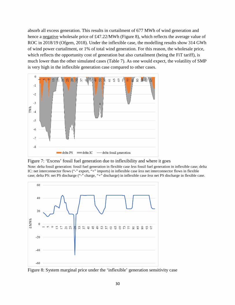
Figure 7 shows differences in coal and gas generation (‘delta fossil generation’), PS net charge (‘delta PS’) and net interconnector flows (‘delta IC’) between inflexible and flexible cases for a sample of the first 100 hours in January. One can see that the ‘excess’ (or the difference) in coal and gas generation is being absorbed by interconnector and PS. Interesting to note is that in hour 29 one can see that combined export and PS charge capacity is not enough to

30

absorb all excess generation. This results in curtailment of 677 MWh of wind generation and hence a negative wholesale price of £47.22/MWh (Figure 8), which reflects the average value of ROC in 2018/19 (Ofgem, 2018). Under the inflexible case, the modelling results show 314 GWh of wind power curtailment, or 1% of total wind generation. For this reason, the wholesale price, which reflects the opportunity cost of generation but also curtailment (being the FiT tariff), is much lower than the other simulated cases (Table 7). As one would expect, the volatility of SMP is very high in the inflexible generation case compared to other cases.

Figure 7: ‘Excess’ fossil fuel generation due to inflexibility and where it goes Note: delta fossil generation: fossil fuel generation in flexible case less fossil fuel generation in inflexible case; delta IC: net interconnector flows (“-” export, “+” imports) in inflexible case less net interconnector flows in flexible case; delta PS: net PS discharge (“-” charge, “+” discharge) in inflexible case less net PS discharge in flexible case.

Figure 8: System marginal price under the ‘inflexible’ generation sensitivity case

31

Lastly, the results from the LP optimization problem confirms our hypothesis that its

results will look like the results from the flexible case but more extreme – ignoring all the unit commitment constraints we find that although PS is hardly utilized, its variation is actually very high, suggesting very volatile PS utilization if a power system were to be completely flexible. However, rather surprisingly we found that the LP solution gives an average SMP which is higher than the SMP under the cases with the unit commitment constraints. This is because in the LP case, there are more interconnector imports and gas is dispatched more than coal. That said, the total operating cost of the system is the lowest — not surprisingly UC constraints have a cost.

4.5. A case study: a simple economic analysis of hydro pumped storage As a case study we look at a simple analysis of the impact of wind generation on the

profitability of PS in the GB electricity market. For this, we measure the impact of wind on PS private cost and benefit by varying wind production by 50% up (and down) from the actual 2015 production level (baseline). Varying wind production changes the residual demand to be met by conventional generation and PS but also changes the operating reserve requirement (Appendix 1, A.3). Both changes could substantially impact PS through price arbitrage opportunities as well as a balancing tool.

Annual profit, 𝑅𝑅𝑗𝑗,𝑡𝑡𝑃𝑃𝑃𝑃, for PS units are defined as profit from price arbitrage (first term) and

received payments from the provision of spinning up reserve (second term) less ongoing fixed O&M as well as transmission grid connection costs (FCj):

𝑅𝑅𝑗𝑗𝑃𝑃𝑃𝑃 = ���𝑑𝑑𝑗𝑗,𝑡𝑡∗ �𝑝𝑝𝑡𝑡∗ − 𝐶𝐶𝑗𝑗𝑉𝑉𝑉𝑉𝑅𝑅� − 𝑐𝑐𝑗𝑗,𝑡𝑡

∗ 𝑝𝑝𝑡𝑡∗�8760

𝑡𝑡=1

� + �� 𝑟𝑟𝑟𝑟𝑗𝑗,𝑡𝑡∗ 𝑝𝑝𝑡𝑡

∗8760

𝑡𝑡=1

� + (𝑉𝑉𝑗𝑗,8760 − 𝑉𝑉𝑗𝑗,1) − 𝐹𝐹𝐶𝐶𝑗𝑗 (26)

where * denotes optimal values from the solution to the unit commitment problem, 𝑝𝑝𝑡𝑡∗ is the system marginal price, 𝑝𝑝𝑡𝑡

∗ is the spinning up reserve price, 𝑉𝑉𝑗𝑗,1 is the value of energy stored in the first time period valued at the wholesale price of that time period, and 𝑉𝑉𝑗𝑗,8760 is the value of energy stored in the last time period valued at the price of that time period. All other parameters and variables are as in the notation section (see §3.1) and in Appendix 1 (see §A.5).

Table 8 reports the resulting modelling results. PS profitability improves with more wind on the system. Surprisingly, a 50% wind increase or decrease did not change interconnector flows much in total (although the pattern over different links does change). This suggests that the GB generation system is flexible enough to respond to changes in wind without causing dramatic changes to the total interconnector flows, at least given the 2015 wholesale prices in the interconnected markets. This is despite a 50% increase in wind generation relative to the 2015 level of about 60 TWh, which, together with natural flow hydro and solar PV generation, is about 23% of total net electricity supply in 2015.12

12 Also, this 60 TWh of wind generation is about 20% in final consumption in 2017.

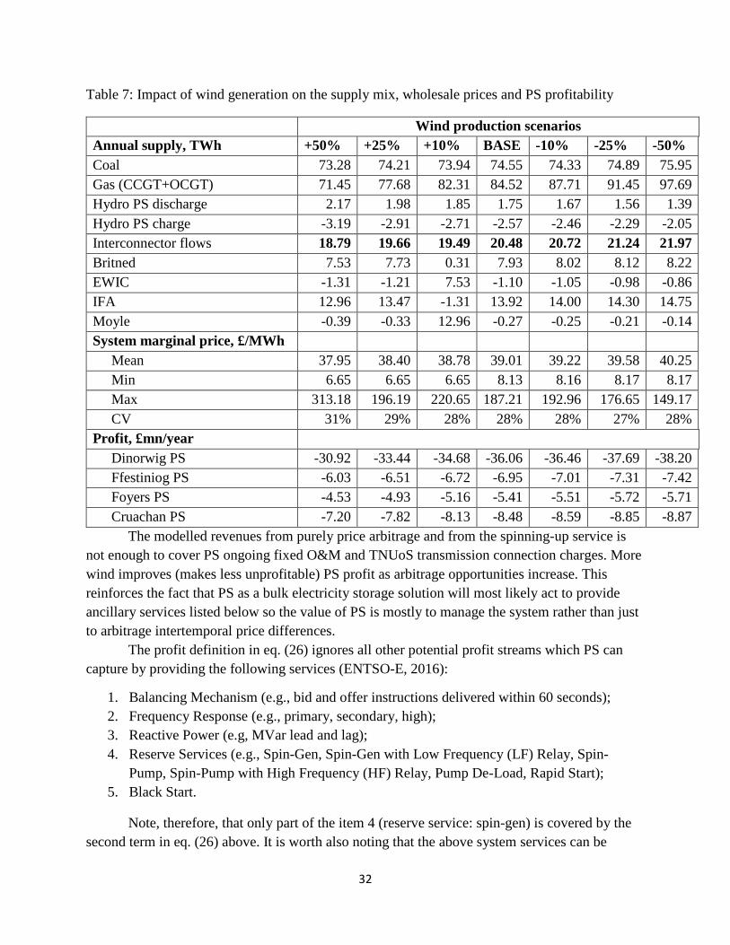
32

Table 7: Impact of wind generation on the supply mix, wholesale prices and PS profitability

Wind production scenarios Annual supply, TWh +50% +25% +10% BASE -10% -25% -50% Coal 73.28 74.21 73.94 74.55 74.33 74.89 75.95 Gas (CCGT+OCGT) 71.45 77.68 82.31 84.52 87.71 91.45 97.69 Hydro PS discharge 2.17 1.98 1.85 1.75 1.67 1.56 1.39 Hydro PS charge -3.19 -2.91 -2.71 -2.57 -2.46 -2.29 -2.05 Interconnector flows 18.79 19.66 19.49 20.48 20.72 21.24 21.97 Britned 7.53 7.73 0.31 7.93 8.02 8.12 8.22 EWIC -1.31 -1.21 7.53 -1.10 -1.05 -0.98 -0.86 IFA 12.96 13.47 -1.31 13.92 14.00 14.30 14.75 Moyle -0.39 -0.33 12.96 -0.27 -0.25 -0.21 -0.14 System marginal price, £/MWh

Mean 37.95 38.40 38.78 39.01 39.22 39.58 40.25 Min 6.65 6.65 6.65 8.13 8.16 8.17 8.17 Max 313.18 196.19 220.65 187.21 192.96 176.65 149.17 CV 31% 29% 28% 28% 28% 27% 28%

Profit, £mn/year Dinorwig PS -30.92 -33.44 -34.68 -36.06 -36.46 -37.69 -38.20 Ffestiniog PS -6.03 -6.51 -6.72 -6.95 -7.01 -7.31 -7.42 Foyers PS -4.53 -4.93 -5.16 -5.41 -5.51 -5.72 -5.71 Cruachan PS -7.20 -7.82 -8.13 -8.48 -8.59 -8.85 -8.87

The modelled revenues from purely price arbitrage and from the spinning-up service is not enough to cover PS ongoing fixed O&M and TNUoS transmission connection charges. More wind improves (makes less unprofitable) PS profit as arbitrage opportunities increase. This reinforces the fact that PS as a bulk electricity storage solution will most likely act to provide ancillary services listed below so the value of PS is mostly to manage the system rather than just to arbitrage intertemporal price differences.

The profit definition in eq. (26) ignores all other potential profit streams which PS can capture by providing the following services (ENTSO-E, 2016):

1. Balancing Mechanism (e.g., bid and offer instructions delivered within 60 seconds); 2. Frequency Response (e.g., primary, secondary, high); 3. Reactive Power (e.g, MVar lead and lag); 4. Reserve Services (e.g., Spin-Gen, Spin-Gen with Low Frequency (LF) Relay, Spin-

Pump, Spin-Pump with High Frequency (HF) Relay, Pump De-Load, Rapid Start); 5. Black Start.

Note, therefore, that only part of the item 4 (reserve service: spin-gen) is covered by the second term in eq. (26) above. It is worth also noting that the above system services can be

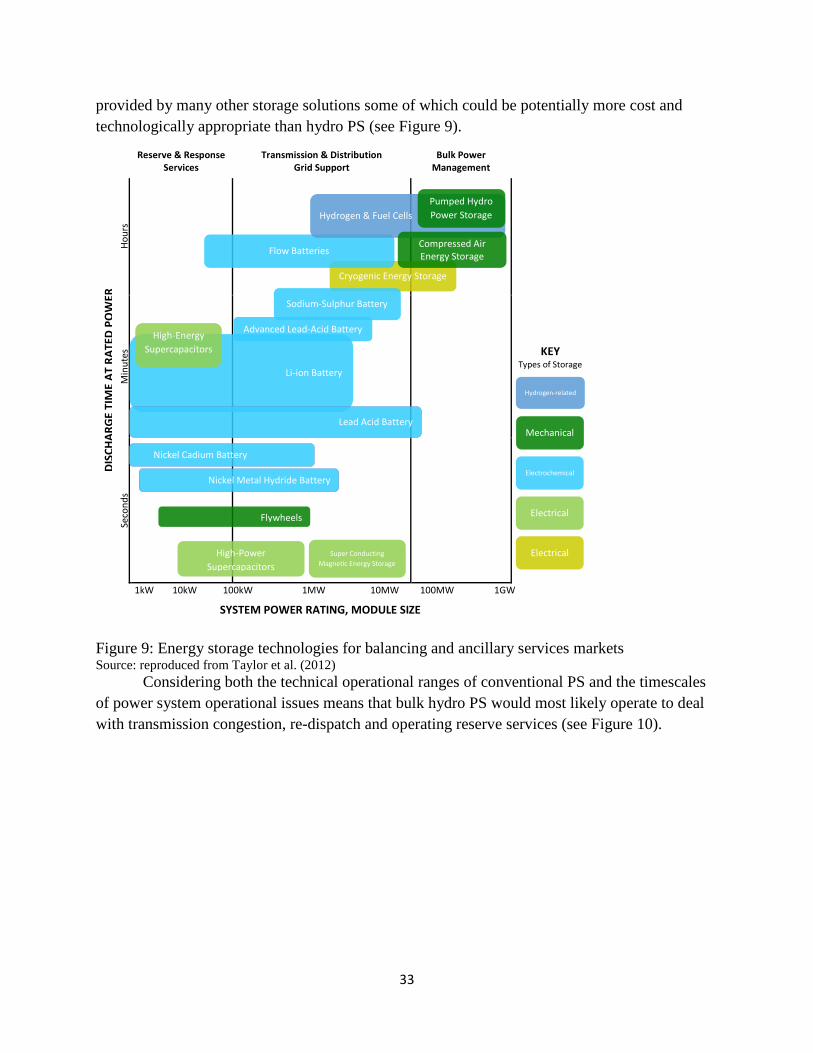
33

provided by many other storage solutions some of which could be potentially more cost and technologically appropriate than hydro PS (see Figure 9).

Figure 9: Energy storage technologies for balancing and ancillary services markets Source: reproduced from Taylor et al. (2012)

Considering both the technical operational ranges of conventional PS and the timescales of power system operational issues means that bulk hydro PS would most likely operate to deal with transmission congestion, re-dispatch and operating reserve services (see Figure 10).

Reserve & Response Services

Transmission & Distribution Grid Support

Bulk Power Management

DISC

HARG

E TI

ME

AT R

ATED

PO

WER

Ho

urs

KEY Types of Storage

Min

utes

Seco

nds

1kW 10kW 100kW 1MW 10MW 100MW 1GW SYSTEM POWER RATING, MODULE SIZE

Cryogenic Energy Storage

Flow Batteries

Sodium-Sulphur Battery

Advanced Lead-Acid Battery

Li-ion Battery

Lead Acid Battery

Nickel Cadium Battery

Nickel Metal Hydride Battery

High-Energy Supercapacitors

Flywheels

High-Power Supercapacitors

Super Conducting Magnetic Energy Storage

Hydrogen-related

Mechanical

Electrochemical

Hydrogen & Fuel Cells Pumped Hydro Power Storage

Compressed Air Energy Storage

Electrical

Electrical

34

Figure 10: PS technologies for balancing and ancillary services markets Source: reproduced from DNV GL (2016).

In 2015-2018 financial years, total costs of managing constraint averaged about £350 mn/year, or about 37% of the total balancing costs of the GB electricity system. Managing transmission constraints is the most expensive item in the balancing and ancillary services markets. Figure 11 gives breakdown of this cost by fuel and payment types.

Figure 11: breakdown of constraint costs by fuel type (2015-2018 Financial Years)

35

Note: Payment to manage constraints is the cost incurred by National Grid to pay generators to be constrained off whereas payment to rebalance the system is the cost incurred by National Grid to bring the system back into balance, which includes not just energy balance, but also to readdress the level of reserve available on the system. Source: National Grid (2019)

We can see that, on average, gas receives 60% of the total constraint management payment, of which 57% is to rebalance the system; whereas coal receives about 13% of the net constraint payment. The category “others” contains all fuel types not reported separately and includes PS, hydro, OCGT, demand side response, nuclear and oil. Thus, PS would have received not more than 6% of the constraint payments, on average, in 2015-18, or at most £20 mn/year in total. Unsurprisingly, given their wide geographic spread and flexibility, gas power stations dominate re-dispatch to deal with transmission constraints.

PS stations are, however, active in fast reserve, response and other reserve services with a combined market share of 30% in all these three ancillary services (Figure 12: right panel). The total monthly payment for all three services in the period April 2018 – Feb 2019 was about £5.7 mn/month, of which 87% is the payment for fast reserve service (Figure 12: left panel). Apart from these reserve and response services PS can offer black start capability as well as reactive power services.

Figure 12: hydro PS market share in reserve and response services (left panel) and monthly average payments (right panel) (April 2018 – Feb 2019) Source: National Grid (2019)

If we add to the modelled revenue from price arbitrage the actual 2018 balancing and ancillary services revenues (Figure 12) against the ongoing fixed O&M and transmission connection costs, then PS seem to be profitable under the baseline and higher wind production scenarios (Figure 13). However, revenues would not be enough to cover capex of a new 600 MW PS station. Investment in new PS will be challenging and the gap in financing will have to come from other balancing and ancillary services market opportunities rather than purely price arbitrage even with a very high share of VRE. We see that the four existing PS stations can recover their ongoing costs and that majority of the revenue to cover the costs comes from

36

balancing and ancillary services markets – about 75% – whereas only 25% comes from price arbitrage.

Figure 13: Hydro PS revenue streams and costs Note: capex annuity calculated assuming a 10% discount rate and 50 years of operation; capex includes pre-licensing, regulatory, overnight construction capital and infrastructure costs (see Leigh Fisher & Jacobs (2016) report, medium values).

The unit commitment model with hourly resolution can reasonably capture the price arbitrage value of PS but analysing the economics of electrical energy storage in the context of growing VRE production would require a robust analysis of revenue opportunities in the balancing and ancillary services markets, which would require a considerably more demanding stochastic model. Its calibration would require access to market information currently rather limited. Thus, the breakdown in payments received by PS (as in Figure 12) in GB only became available rather recently. Other services like black start, reactive power etc. have no detailed breakdown in terms of who is providing what.

Transmission congestion management is provided mostly by gas and less so by coal. PS competes with gas (and less so with coal) in providing flexibility capability. Whether PS adds or reduces conventional generation’s value is therefore not immediately clear. To consider the potential portfolio effect of combining PS with conventional generation we run the model with all possible combinations (Table 9) of the existing four PS stations to measure impacts on profitability of conventional generation as well as on overall system operating cost. We calculate the average marginal contribution (Shapley, 1953) of each PS station to gas and coal profitability and to total system operating cost. Table 8: PS sensitivities – all possible combinations of existing stations in the market

37

Sensitivity Dinorwig Ffestiniog Foyers Cruachan

Total power (MW)

Total energy capacity (GWh)

1 ✓ 1728 9.1 2 ✓ 360 1.3 3 ✓ 300 6.3 4 ✓ 440 7.2 5 ✓ ✓ 2,088 10.4 6 ✓ ✓ 2,028 15.4 7 ✓ ✓ 2,168 16.3 8 ✓ ✓ 660 7.6 9 ✓ ✓ 800 8.5 10 ✓ ✓ 740 13.5 11 ✓ ✓ ✓ 2,388 16.7 12 ✓ ✓ ✓ 2,528 17.6 13 ✓ ✓ ✓ 1,100 14.8 14 ✓ ✓ ✓ 2,468 22.6

Baseline ✓ ✓ ✓ ✓ 2,828 23.9 Note: each of this sensitivity was modelled under the baseline case.

Figure 14 summarise our findings while detailed calculations of marginal values of each PS is in Appendix 2 (Table A. 10 - Table A. 13).

38

Figure 14: Average marginal contribution of each PS stations to gas and coal generation and to the overall GB electricity system

All four stations reduce total system operating cost, with higher power output PS units contributing more to minimising the total system cost. On the other hand, the higher is the power output of a PS the larger is the negative impact on gas and coal profitability – PS competes with gas (and coal) in providing flexibility, except. interestingly, Ffestiniog that delivers a positive impact on gas and coal profitability. Thus, a relatively small PS could potentially improve the profitability of the existing (2015) gas and coal generation fleet in GB, while large storage units compete with existing gas and coal generation. From a system cost minimization point of view, any of the four existing storage units provide extra value and the higher is the power output the more valuable it is to the system.

5. Conclusions This paper outlined a moderately simple unit commitment and economic dispatch model

and applied it to the GB electricity market. The model reproduced the 2015 market data reasonably well on average, without applying hourly calibration parameters. Instead, the calibration only used multiplicative fuel mix calibration parameters and applied it for the entire modelling horizon (8760 hours or one year). Multiplicative calibration parameters address systematic biases in the input data, as well as systematic biases inherent in the modelling approach, such as determinism and perfect foresight. In this regard, using this multiplicative correction biases parameter for sensitivity and further scenario-based analysis is more plausible than hourly mark-up parameters calibrated to historical data.

Using this calibrated (to the 2015 GB electricity market) baseline result we carried out a number of sensitivity analyses to test the robustness of the model against changes in model structure, its main assumptions and data inputs. First, we tested performance and results against different model horizon lengths. The performance and the solution time of the calibrated model is quite sensitive to the length of the modelling horizon. Increasing the length of the modelling horizon reduces its ‘compactness’ – the model becomes huge. Increasing the model horizon has a dramatic increase in the solution time without any meaningful improvement in the ‘quality’ of the results. This highlights the importance of model compactness and its influence on the solution time. Fortunately, the model outputs are very robust to variations in the model time horizon.

The next sensitivity test dealt with operating reserve requirements (both spin-up and down reserves). Here, a higher volatility of reserve requirements means a higher utilization of PS. Higher wind and solar penetration will likely increase the requirement for electric energy storage, but more as a balancing and ancillary service provider rather than as purely price arbitrage. Further, when we restrict PS to provide (non-synchronised) spin-up capability only, its utilization is very close to the actual 2015 level underlying its importance in providing balancing and ancillary services. However, excluding gas-fired (non-synchronised) units from providing spin-up reserve means a very high SMP volatility as this puts a substantial pressure on synchronized units (coal and gas units who are already committed in the energy only market) as

39

well as PS to fulfil reserve requirements. In all our sensitivity cases, non-synchronized gas-fired capacity will cover 99% of all spin-up reserve requirements. It is only when we exclude non-synchronized gas is the spin-up reserve market roughly equally divided between online coal and gas units. All in all, defining operating reserve requirements is important as it will influence the dispatch order and SMPs. That said, our analysis shows that the variations in annual output of gas and coal is of order of 4% and 7% respectively and 80% for PS. Clearly the impact of operating reserve requirements on PS utilization is proportionately the greatest.

We also tested the model’s structural features related to plant flexibility, namely, ramping rates and commitment time, as well as start-up and shut-down decisions and their associated costs. We found that cycling characteristics (ramp rate and commitment time) can change the supply mix quite significantly. Coal’s inflexibility disadvantages gas in the supply mix due to minimum up and down time requirements of coal plants and thus their inability to respond to fuel price dynamics quickly. Further, we found that total system operating cost under a simple economic dispatch model that ignores all the unit commitment and cycling decisions is just 2.7% less than the operating cost of the system under a UC model. The majority of cost savings is due to lower fuel and carbon costs. Start-up and shut-down costs represent just under 0.3% of total operating cost of the system. Hence, the impact of cycling is not so much on operating costs per se but on the way plants react to changes in demand and supply conditions and system marginal prices.

Finally, as a case study we carried out a simple economic analysis of the four existing GB PS stations. More wind increases PS arbitrage revenue – specifically, with every percentage point increase in wind capacity the total PS arbitrage profit increases by 0.21 percentage points. Although in absolute terms, under a range of wind capacities, PS modelled revenue from price arbitrage is not enough to cover its ongoing fixed O&M and transmission connection charges. This reinforces the conclusion that PS has most value for providing balancing and ancillary services. This is confirmed from the 2015-18 GB balancing and ancillary services data, which suggests that PS stations were not active in managing transmission constraints, where about 60% of constraint payments went to gas-fired units. GB Gas stations dominate re-dispatch to deal with transmission constraints due to their geographic distribution and operational flexibility. However, PS stations are active in providing ancillary services such as fast reserve, response and other reserve services. In the 2018/19 financial year they had a combined market share of 30% in all these three services. Adding the modelled revenue from price arbitrage to the 2018 balancing and ancillary services revenues and subtracting the ongoing fixed O&M and transmission connection costs suggests that the four existing PS stations are profitable. Most of the revenue to cover the costs comes from balancing and ancillary services markets – about 75% – whereas only 25% comes from price arbitrage.

However, the revenues would not be enough to justify a new 600 MW PS station, making investment in any new PS challenging. The gap in financing a new PS facility will have to come from balancing and ancillary services market opportunities and less from purely price arbitrage. This is true even with a very high share of VRE, unless a substantial portion of conventional generation capacity, especially gas, comes off line. This is because the existing PS competes with gas (and with coal) in providing flexibility such as ramping. Put differently, the 2015 supply mix in GB has enough flexibility to deal with an increase of 50% of wind capacity. The marginal

40

contribution of most (but not the smallest) existing PS stations is to reduce gas and coal profitability, while reducing the total system operating cost.

To conclude, the unit commitment model with hourly resolution can reasonably capture the price arbitrage value of PS but analysing the economics of electrical energy storage requires a robust analysis of revenue opportunities in the balancing and ancillary services markets. Thus, for future research, it would be desirable to include ancillary services as well as conventional plant re-dispatch to deal with transmission constraints which requires explicitly dealing with forecast and plant uncertainty (especially VRE) over different time scales. However, the curse of dimensionality of stochastic models and more importantly data availability for calibration purposes might limit research in this direction. The final point to stress is that the model assumes perfect competition, and is not well-designed to deal with the exercise of market power. Incorporating market power in a traditional UC models, such as this, would potentially lead to an equilibrium problem with equilibrium constraints (EPEC) which, with just continuous decision variables, is well-known to be an extremely hard problem to solve.

41

6. References Abujarad, S. Y., Mustafa, M. W., and Jamian, J. J. (2017). "Recent approaches of unit

commitment in the presence of intermittent renewable energy resources: A review", Renewable and Sustainable Energy Reviews, 70, pp.215–223.

Andersen, K.S., Termansen, L.B., Gargiulo, M., Gallachóir, B.O. (2019) “Bridging the gap using energy services: Demonstrating a novel framework for soft linking top-down and bottom-up models,” Energy, vol. 169, pp. 277-293. https://doi.org/10.1016/j.energy.2018.11.153

Annicchiarico, B., Battles, S., Dio, F.D., Molina, P., Zoppoli, P. (2016). “GHG mitigation schemes and energy policies: A model-based assessment for the Italian economy,” Economic Modelling, vol. 61, pp. 495-509

Arroyo, J. M. and Conejo, A. J. (2000). “Optimal response of a thermal unit to an electricity spot market”, IEEE Transactions on power systems, Vol. 15, No 3, 2000, pp.1098–1104.

BEIS (Department for Business, Energy & Industrial Strategy) (2016). “Greenhouse gas reporting - Conversion factors 2016”. Available at: https://www.gov.uk/government/publications/greenhouse-gas-reporting-conversion-factors-2016 (Accessed March 2019)

Carrión, M. and Arroyo, J. M. (2006). “A computationally efficient mixed-integer linear formulation for the thermal unit commitment problem”, IEEE Transactions on power systems, Vol. 21, No 3, 2006, pp.1371–1378.

CCC (Committee on Climate Change) (2016). “UK climate change following the Paris Agreement”. Available at: https://www.theccc.org.uk/wp-content/uploads/2016/10/UK-climate-action-following-the-Paris-Agreement-Committee-on-Climate-Change-October-2016.pdf (Accessed March 2019)

CCC (2018). “Reducing UK emissions - 2018 Progress Report to Parliament", a report by Committee on Climate Change, June 2018. Available at: https://www.theccc.org.uk/wp-content/uploads/2018/06/CCC-2018-Progress-Report-to-Parliament.pdf (Accessed March 2019)

Cebulla, F., and Fichter, T. (2017). “Merit order or unit-commitment: How does thermal power plant modeling affect storage demand in energy system models?,” Renew. Energy, vol. 105, no. December, pp. 117–132.

Chase, D. L. and Kehoe, P. T. (2014). “GE Combined-Cycle Product Line and Performance,” GE Power Systems, 2014. Available at: http://physics.oregonstate.edu/~hetheriw/energy/topics/doc/elec/natgas/cc/combined%20cycle%20product%20line%20and%20performance%20GER3574g.pdf (Accessed March 2019)

Chyong, C.K., Guo, B.W., Newbery, D. (2019). “The impact of a Carbon Tax on the CO2 emissions reduction of wind”. EPRG Working Paper N1904, January 2019, available at: https://www.eprg.group.cam.ac.uk/eprg-working-paper-1904/ (Accessed July 2019)

Chyong, C.K., Pollitt, M., and Cruise, R. (2019). “Can wholesale electricity prices support “subsidy-free” generation investment in Europe?”, EPRG Working Paper Series N1919, available at: https://www.eprg.group.cam.ac.uk/eprg-working-paper-1919/ (Accessed July 2019).

Damcı-Kurt, P., Küçükyavuz, S., Rajan, D., Atamtürk, A. (2015). “A Polyhedral study of production ramping”, Mathematical Programming, Vol. 158, Issue 1-2, pp.158–175. https://doi.org/10.1007/s10107-015-0919-9

42

Denholm, P., Jorgenson, J., Hummon, M., Jenkin, T., Palchak, D., Kirby, B., Ma, O., O'Malley, M. (2013). "The Value of Energy Storage for Grid Applications the Value of Energy Storage for Grid Applications," NREL technical report. Available at: https://www.nrel.gov/docs/fy13osti/58465.pdf (Accessed March 2019)

Dixon, P.B., Rimmer, M.T., and Waschik, R. (2017) “Linking CGE and specialist models: Deriving the implications of highway policy using USAGE-Hwy,” Economic Modelling, vol. 66, pp. 1-18. https://doi.org/10.1016/j.econmod.2017.04.022

DNV GL (2016). “The Benefits of Pumped Storage Hydro to the UK”, a report for Scottish Renewables. Available at: https://www.scottishrenewables.com/publications/benefits-pumped-storage-hydro-uk/ (Accessed March 2019)

DUKES (Digest of UK Energy Statistics), (2018). 'Digest of UK Energy Statistics (DUKES) 2018: electricity'. Available at: https://www.gov.uk/government/statistics/electricity-chapter-5-digest-of-united-kingdom-energy-statistics-dukes (Accessed August 2018)

ENTSO-E (European Network of Transmission System Operators for Electricity). (2004). “Operation handbook”, Appendix 1, Load-Frequency Control and Performance. Available at: https://www.entsoe.eu/fileadmin/user_upload/_library/publications/entsoe/Operation_Handbook/Policy_1_final.pdf (Accessed March 2019)

ENTSO-E (2016). “Ten Year Network Development Plan 2016. Storage Projects Assessment Sheet” available at: https://docstore.entsoe.eu/Documents/TYNDP%20documents/TYNDP%202016/projects/TYNDP16_Storage_Pr.%20Assessment%20Sheets.pdf (Accessed March 2019)

Morales-España, G., Latorre, J., and Ramos, A. (2013). “Tight and Compact MILP Formulation for the Thermal Unit Commitment Problem,” IEEE Transactions on Power Systems, vol. 28, no. 4, pp. 4897–4908

Gerber, A., Ekanayake, J.B., Awad, B., and Jenkins, N. (2011). “Operation of the 2030 GB power generation system,”, Proceedings of the Institution of Civil Engineers - Energy, vol. 164, pp. 25–37.

GridWatch (2019). “GridWatch Database”. Available at: http://www.gridwatch.templar.co.uk/download.php (Accessed March 2019)

Hach, D., Chyong, C.K., and Spinler, S. (2016). “Capacity market design options: A dynamic capacity investment model and a GB case study,” European Journal of Operational Research, vol. 249, no. 2, pp. 691–705.

Hall, L. M. H. and Buckley, A.R. (2016) “A review of energy systems models in the UK: Prevalent usage and categorisation,” Applied Energy, vol. 169, pp. 607–628.

Henry Chen, Y.-H., Paltsev, S., Reilly, J.M., Morris, J.F., Babiker, M.H. (2016). “Long-term economic modeling for climate change assessment,” Economic Modelling, vol. 52, Part B, pp. 867-883. https://doi.org/10.1016/j.econmod.2015.10.023

Hemmati, R., and Saboori, H. (2016). “Short-term bulk energy storage system scheduling for load leveling in unit commitment : modeling , optimization , and sensitivity analysis,” Journal of Advanced Research, vol. 7, no. 3, pp. 360–372.

HM Government (2010). "2050 Pathways Analysis", pp. 1–252. Available at: https://assets.publishing.service.gov.uk/government/uploads/system/uploads/attachment_data/file/68816/216-2050-pathways-analysis-report.pdf (Accessed March 2019)

Hobbs, B.F. , Rothkopf, M.H., O’Neill, R.P. and Chao, H.-P. (2001). “The next generation of electric power unit commitment models”. Springer. DOI: 10.1007/b108628

43

Holttinen, H. (2005). “Impact of hourly wind power variations on the system operation in the Nordic Countries,” Wind Energy 8(2), pp. 197–218.

Hourcade, J. C., M. Jaccard, C. Bataille and F. Ghersi (2006). "Hybrid modeling: New answers to old challenges - Introduction to the special issue of The Energy Journal." Energy Journal, Vol. 27, Special Issue: Hybrid Modeling of Energy-Environment Policies: Reconciling Bottom-up and Top-down (2006), pp. 1-11.

Huang Y., Pardalos P.M., Zheng Q.P. (2017). “Deterministic Unit Commitment Models and Algorithms”. In: Electrical Power Unit Commitment. SpringerBriefs in Energy. Springer, Boston, MA. https://doi.org/10.1007/978-1-4939-6768-1_2

IPCC (2001) “Climate Change 2001: Mitigation,” A Report of Working Group III of the Intergovernmental Panel on Climate Change, Section 7.6.3: “Top-down and bottom-up models”. Available at: http://www.ipcc.ch/ipccreports/tar/wg3/index.php?idp=310 (Accessed July 2017)

Kompas, T., and Ha, P.H. (2018). “The ‘curse of dimensionality’ resolved: The effects of climate change and trade barriers in large dimensional modelling,” Economic Modelling, in press, available online: https://doi.org/10.1016/j.econmod.2018.08.011

Knueven, B., Ostrowski, L., and Watson, J-P. (2018). “On Mixed Integer Programming Formulations for the Unit Commitment Problem”, E-print, Department of Industrial and Systems Engineering University of Tennessee, Knoxville, TN 37996, November 2018. Available at: http://www.optimization-online.org/DB_HTML/2018/11/6930.html (Accessed July 2019)

Kumar, N., Besuner, P., Lefton, S., Agan, D., and Hilleman, D. (2012). “Power Plant Cycling Costs,” NREL Technical Report, April, 2012. Available at: https://www.nrel.gov/docs/fy12osti/55433.pdf (Accessed March 2019).

Leigh Fisher and Jacobs (2016), “Electricity Generation Costs and Hurdle Rates – Lot 3: Non-Renewable Technologies,” a report prepared for Department of Energy and Climate Change, August, 2016. Available at: https://assets.publishing.service.gov.uk/government/uploads/system/uploads/attachment_data/file/566803/Leigh_Fisher_Non-renewable_Generation_Cost.pdf (Accessed March 2019)

Loulou, R., Goldstein, G., and Noble, K. (2004). “Documentation for the MARKAL Family of Models,” International Energy Agency, (October), pp. 1–389.

Magnago, F.H., Alemany, J., and Lin, J. (2015). “Electrical Power and Energy Systems Impact of demand response resources on unit commitment and dispatch in a day-ahead electricity market,” International Journal of Electrical Power & Energy Systems, vol. 68, pp. 142–149.

MIT Energy Initiative (2016). "Utility of the Future," a report by MIT Energy Initiative. Available at: https://energy.mit.edu/wp-content/uploads/2016/12/Utility-of-the-Future-Full-Report.pdf (Accessed March 2019)

National Grid (2015). “Electricity Ten Year Statement 2015,” Electricity Ten Year Statement 2015, Appendix F Generation Data. Available: https://www.nationalgrideso.com/document/47041/download (Accessed March 2019)

National Grid (2018a), “National Demand Data Explorer,” Demand Data 2011 - 2016. Available: https://www.nationalgrid.com/uk/electricity/market-and-operational-data/data-explorer (Accessed August 2018)

44

National Grid (2018b). “Demand Forecasting Reporting Period: 4th Dec 2017 – 11th Mar 2018”. Available at: https://www.nationalgrid.com/sites/default/files/documents/Quarterly%20Forecasting%20Report%20-%20March18.pdf (Accessed March 2019)

National Grid (2019). “System balancing reports”. Available at: https://www.nationalgrideso.com/balancing-data/system-balancing-reports (Accessed April 2019)

NERC (National Environmental Research Council) (2017). "Glossary of Terms Used in NERC Reliability Standards". Available at: https://www.nerc.com/files/glossary_of_terms.pdf (Accessed March 2019)

Newbery, D.M. (2001). “Privatization, Restructuring, and Regulation of Network Utilities”, MIT Press

Ofgem (The Office of Gas and Electricity Markets) (2015). “Making the electricity system more flexible and delivering the benefits for consumers”, Ofgem’s Position Paper. Available at: https://www.ofgem.gov.uk/ofgem-publications/96959/flexibilitypositionpaperfinal-pdf (Accessed March 2019)

Ofgem (2017). 'Final proposals for electricity System Operator incentives from April 2017'. Available at: https://www.ofgem.gov.uk/system/files/docs/2017/03/final_proposals_for_electricity_system_operator_incentives_from_april_2017.pdf (Accessed March 2019)

Ofgem (2018). “Renewables Obligation (RO) buy-out price and mutualisation ceilings for 2018-19 RO Year”. Available at: https://www.ofgem.gov.uk/publications-and-updates/renewables-obligation-ro-buy-out-price-and-mutualisation-ceilings-2018-19-ro-year (Accessed April 2019)

Pandzžić, H., Dvorkin, Y., Wang, Y., Qiu, T., and Kirschen, D.S., (2014). “Effect of time resolution on unit commitment decisions in systems with high wind penetration,” 2014 IEEE PES Gen. Meet., Conf. Expo., pp. 1–5. DOI: 10.1109/PESGM.2014.6939548.

Panos, E., and Lehtilä, A. (2016). “Dispatching and unit commitment features in TIMES”, International Energy Agency – Energy Technology Systems Analysis Programme (ETSAP). Available at: https://ieaetsap.org/docs/TIMES_Dispatching_Documentation.pdf (Accessed March 2019)

Pfenninger, S., Hawkes, A., and Keirstead, J. (2014). “Energy systems modelling for twenty-first century energy challenges,” Renewable and Sustainable Energy Reviews, 33(June), pp. 74–86.

Pozo, D., Contreras, J., and Sauma, E. (2014). “Unit Commitment with Ideal and Generic Energy Storage Units”, IEEE Transactions on Power Systems, vol. 29, no. 6, pp. 2974–2984.

Pudjianto, D., Aunedi, M., Djapic, P., and Strbac, G. (2014). “Whole-Systems Assessment of the Value of Energy Storage in Low-Carbon Electricity Systems,” IEEE Transactions on Smart Grid, vol. 5, no. 2, pp. 1098–1109.

Pye, S., Li, F. G., Price, J., and Fais, B. (2017). “Achieving net-zero emissions through the reframing of UK national targets in the post-Paris Agreement era,” Nature Energy, 2, pp. 1–7.

Qadrdan, M., Wu, J., Jenkins, N., and Ekanayake, J. (2014). “Operating strategies for a GB integrated gas and electricity network considering the uncertainty in wind power forecasts”. IEEE Transactions on Sustainable Energy, 5(1):128–138.

45

Quoilin, S., Hidalgo Gonzales, I., and Zucker, A. (2017). “Modelling Future EU Power Systems Under High Shares of Renewables”. The Dispa-SET 2.1 open-source model. JRC Technical Report, EU Commission, 2017

Schnellmann, M.A., Chyong, C.K., Reiner, D.M., Scott, S.A. (2018). “Deploying gas power with CCS: The role of operational flexibility, merit order and future energy scenarios”. EPRG Working Paper N1836, November 2018, available at: https://www.eprg.group.cam.ac.uk/eprg-working-paper-1836/ (Accessed July 2019)

Schröder, A., Kunz, K., Meiss, J., Mendelevitch, R., and von Hirschhausen, C. (2013). “Current and Prospective Costs of Electricity Generation until 2050”. DIW Data Documentation 68. Available at: https://www.diw.de/documents/publikationen/73/diw_01.c.424566.de/diw_datadoc_2013-068.pdf (Accessed August 2018)

Scottish Power (2011). 'Cruachan Power Station: site information'. Available at: https://www.scottishpower.com/userfiles/file/CruachanSiteComplete2011.pdf (Accessed March 2019)

SEM (The Single Electricity Market for the island of Ireland) (2017). “SEM Monitoring Report: Q1 2017”, SEM-17-035, May 2017, p.22. Available at: https://www.semcommittee.com/sites/semcommittee.com/files/media-files/SEM-17-034%20MMU%20Public%20Report%20Q1%202017.pdf (Accessed May 2019)

Shapley, L.S. (1953). “A value for n-person games,” Annals of Mathematical Studies, No. 28, pp. 307–317.

Spataru, C., Drummond, P., Barrett, M., and Emes, M. (2013). "Common Road to 2050: Energy Networks and Policy (ENP2050)", a study at UCL Energy Institute. Available at: https://www.ucl.ac.uk/energy-networks-policy/docs/FinalReportENP.pdf (Accessed March 2019)

Strachan, N. (2011). “Business-as-Unusual: Existing policies in energy model baselines,” Energy Economics, 33(2), pp.153–160.

Takriti, S., Birge, J. R. and Long, E. (1996). "A stochastic model for the unit commitment problem," in IEEE Transactions on Power Systems, vol. 11, no. 3, pp. 1497-1508, Aug. 1996. doi: 10.1109/59.535691

Takriti, S., Krasenbrink, B., Wu, L. S.-Y. (2000). “Incorporating Fuel Constraints and Electricity Spot Prices into the Stochastic Unit Commitment Problem”, Operations Research, 48(2), pp.268–280. https://doi.org/10.1287/opre.48.2.268.12379

Tapia-Ahumada, K., Octaviano, C., Rausch, S., Pérez-Arriaga, I. (2015). “Modeling intermittent renewable electricity technologies in general equilibrium models,” Economic Modelling, vol. 51, pp. 242-262. https://doi.org/10.1016/j.econmod.2015.08.004

Taylor, P., Bolton, R., Stone, D., Zhang, X.-P., Martin, C., and Upham, P., (2012). “Pathways for energy storage in the UK”. A report for the Centre for Low Carbon Futures. Available at: http://oro.open.ac.uk/40087/2/Pathways_for_Energy_Storage_in_the_UK.pdf (Accessed March 2019)

Townsend, A.K., (2013). “A Grid-Level Assessment of Compressed Air Energy Storage in ERCOT,” PhD Thesis, The University of Texas at Austin. Available at: https://repositories.lib.utexas.edu/bitstream/handle/2152/22104/townsend_dissertation_20132.pdf?sequence=1&isAllowed=y (Accessed March 2019)

46

Van Den Bergh, K., and Delarue, E. (2015). “Cycling of conventional power plants: Technical limits and actual costs,” Energy Conversion and Management, vol. 97, no. March, pp. 70–77.

Vijay, A., Fouquet, N., Staffell, A., and Hawkes, A. (2017). “The value of electricity and reserve services in low carbon electricity systems,” Applied Energy, vol. 201, pp. 111–123.

WEC (World Energy Council) (2016). "World Energy Trilemma – 2016: Defining measures to accelerate the energy transition" a report by World Energy Council in partnership with Oliver Wyman. Available at: https://www.worldenergy.org/wp-content/uploads/2016/05/World-Energy-Trilemma_full-report_2016_web.pdf (Accessed March 2019)

Wene, C. O. (1996). "Energy-economy analysis: Linking the macroeconomic and systems engineering approaches." Energy 21(9), pp. 809-824.

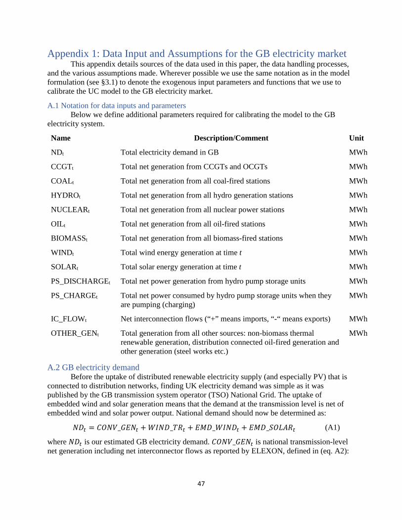
47

Appendix 1: Data Input and Assumptions for the GB electricity market This appendix details sources of the data used in this paper, the data handling processes,

and the various assumptions made. Wherever possible we use the same notation as in the model formulation (see §3.1) to denote the exogenous input parameters and functions that we use to calibrate the UC model to the GB electricity market.

A.1 Notation for data inputs and parameters Below we define additional parameters required for calibrating the model to the GB

electricity system.

Name Description/Comment Unit

NDt Total electricity demand in GB MWh

CCGTt Total net generation from CCGTs and OCGTs MWh

COALt Total net generation from all coal-fired stations MWh

HYDROt Total net generation from all hydro generation stations MWh

NUCLEARt Total net generation from all nuclear power stations MWh

OILt Total net generation from all oil-fired stations MWh

BIOMASSt Total net generation from all biomass-fired stations MWh

WINDt Total wind energy generation at time t MWh

SOLARt Total solar energy generation at time t MWh

PS_DISCHARGEt Total net power generation from hydro pump storage units MWh

PS_CHARGEt Total net power consumed by hydro pump storage units when they are pumping (charging)

MWh

IC_FLOWt Net interconnection flows (“+” means imports, “-“ means exports) MWh

OTHER_GENt Total generation from all other sources: non-biomass thermal renewable generation, distribution connected oil-fired generation and other generation (steel works etc.)

MWh

A.2 GB electricity demand Before the uptake of distributed renewable electricity supply (and especially PV) that is

connected to distribution networks, finding UK electricity demand was simple as it was published by the GB transmission system operator (TSO) National Grid. The uptake of embedded wind and solar generation means that the demand at the transmission level is net of embedded wind and solar power output. National demand should now be determined as:

𝑁𝑁𝐷𝐷𝑡𝑡 = 𝐶𝐶𝐶𝐶𝑁𝑁𝑉𝑉_𝐺𝐺𝑆𝑆𝑁𝑁𝑡𝑡 + 𝑊𝑊𝑊𝑊𝑁𝑁𝐷𝐷_𝑇𝑇𝑅𝑅𝑡𝑡 + 𝑆𝑆𝑀𝑀𝐷𝐷_𝑊𝑊𝑊𝑊𝑁𝑁𝐷𝐷𝑡𝑡 + 𝑆𝑆𝑀𝑀𝐷𝐷_𝑆𝑆𝐶𝐶𝑃𝑃𝑆𝑆𝑅𝑅𝑡𝑡 (A1)

where 𝑁𝑁𝐷𝐷𝑡𝑡 is our estimated GB electricity demand. 𝐶𝐶𝐶𝐶𝑁𝑁𝑉𝑉_𝐺𝐺𝑆𝑆𝑁𝑁𝑡𝑡 is national transmission-level net generation including net interconnector flows as reported by ELEXON, defined in (eq. A2):

48

𝐶𝐶𝐶𝐶𝑁𝑁𝑉𝑉_𝐺𝐺𝑆𝑆𝑁𝑁𝑡𝑡 = 𝐶𝐶𝐶𝐶𝐺𝐺𝑇𝑇𝑡𝑡 + 𝐶𝐶𝐶𝐶𝑆𝑆𝑃𝑃𝑡𝑡 + 𝑊𝑊𝐶𝐶_𝐹𝐹𝑃𝑃𝐶𝐶𝑊𝑊𝑆𝑆𝑡𝑡 + 𝐻𝐻𝐻𝐻𝐷𝐷𝑅𝑅𝐶𝐶𝑡𝑡 + 𝑁𝑁𝑆𝑆𝐶𝐶𝑃𝑃𝑆𝑆𝑆𝑆𝑅𝑅𝑡𝑡 + 𝐶𝐶𝑊𝑊𝑃𝑃𝑡𝑡+ 𝐵𝐵𝑊𝑊𝐶𝐶𝑀𝑀𝑆𝑆𝑆𝑆𝑆𝑆𝑡𝑡 + 𝐶𝐶𝑇𝑇𝐻𝐻𝑆𝑆𝑅𝑅_𝐺𝐺𝑆𝑆𝑁𝑁𝑡𝑡 + 𝑃𝑃𝑆𝑆_𝐷𝐷𝑊𝑊𝑆𝑆𝐶𝐶𝐻𝐻𝑆𝑆𝑅𝑅𝐺𝐺𝑆𝑆𝑡𝑡− 𝑃𝑃𝑆𝑆_𝐶𝐶𝐻𝐻𝑆𝑆𝑅𝑅𝐺𝐺𝑆𝑆𝑡𝑡

(A2)

where 𝑊𝑊𝑊𝑊𝑁𝑁𝐷𝐷_𝑇𝑇𝑅𝑅𝑡𝑡 is transmission level generation from all wind generators as reported by ELEXON (GridWatch, 2019); 𝑆𝑆𝑀𝑀𝐷𝐷_𝑊𝑊𝑊𝑊𝑁𝑁𝐷𝐷𝑡𝑡 is an estimate of the GB wind generation from wind farms which do not have Transmission System metering installed. These wind farms are embedded in the distribution network and “invisible” to National Grid. Their effect is to suppress the electricity demand during periods of high wind. The actual output of these generators is not known so an estimate is provided based on National Grid’s best model (National Grid, 2018). Similarly, the 𝑆𝑆𝑀𝑀𝐷𝐷_𝑆𝑆𝐶𝐶𝑃𝑃𝑆𝑆𝑅𝑅𝑡𝑡 is National Grid’s estimated embedded solar generation lacking transmission system metering. Both embedded wind and solar generation estimated were obtained from the National Grid website (National Grid, 2018).

Finally, the residual demand, Dt, that we model in eq. 2 in the main text is defined as:

𝐷𝐷𝑡𝑡 = 𝑁𝑁𝐷𝐷𝑡𝑡 − (𝑊𝑊𝑊𝑊𝑁𝑁𝐷𝐷_𝑇𝑇𝑅𝑅𝑡𝑡 + 𝑆𝑆𝑀𝑀𝐷𝐷_𝑊𝑊𝑊𝑊𝑁𝑁𝐷𝐷𝑡𝑡 + 𝑆𝑆𝑀𝑀𝐷𝐷_𝑆𝑆𝐶𝐶𝑃𝑃𝑆𝑆𝑅𝑅𝑡𝑡) − (𝐻𝐻𝐻𝐻𝐷𝐷𝑅𝑅𝐶𝐶𝑡𝑡+ 𝑁𝑁𝑆𝑆𝐶𝐶𝑃𝑃𝑆𝑆𝑆𝑆𝑅𝑅𝑡𝑡 + 𝐶𝐶𝑊𝑊𝑃𝑃𝑡𝑡 + 𝐵𝐵𝑊𝑊𝐶𝐶𝑀𝑀𝑆𝑆𝑆𝑆𝑆𝑆𝑡𝑡 + 𝐶𝐶𝑇𝑇𝐻𝐻𝑆𝑆𝑅𝑅_𝐺𝐺𝑆𝑆𝑁𝑁𝑡𝑡) (A3)

or

𝐷𝐷𝑡𝑡 = 𝐶𝐶𝐶𝐶𝐺𝐺𝑇𝑇𝑡𝑡 + 𝐶𝐶𝐶𝐶𝑆𝑆𝑃𝑃𝑡𝑡 + 𝑃𝑃𝑆𝑆𝐷𝐷𝐼𝐼𝑃𝑃𝐶𝐶𝐷𝐷𝑉𝑉𝑅𝑅𝐺𝐺𝐸𝐸𝑡𝑡 − 𝑃𝑃𝑆𝑆𝐶𝐶𝐷𝐷𝑉𝑉𝑅𝑅𝐺𝐺𝐸𝐸𝑡𝑡 + 𝑊𝑊𝐶𝐶_𝐹𝐹𝑃𝑃𝐶𝐶𝑊𝑊𝑆𝑆𝑡𝑡 (A4)

A.3. Operating reserve requirements Gerber et al. (2011) define the positive operating reserve requirement as follows:

3 × �(𝜎𝜎𝐷𝐷𝐹𝐹2 + 𝜎𝜎𝑊𝑊𝐹𝐹2 ) + 1.8𝐺𝐺𝑊𝑊 (A5)

where 𝜎𝜎𝐷𝐷𝐹𝐹is the demand forecast and 𝜎𝜎𝑊𝑊𝐹𝐹 is wind forecast error standard deviation (Holttinen, 2005 as cited in Gerber et al., 2011). Gerber et al. (2011) noted that in a power system without significant variable renewable generation, operating reserve is determined by the capacity of the largest unit on the system as well as by load forecast errors. In their work, they have assumed 1.8 GW as the largest anticipated plant coming on line in 2020 in the GB (the next nuclear power station, not now expected much before 2025). We should note that 𝜎𝜎𝐷𝐷𝐹𝐹and 𝜎𝜎𝑊𝑊𝐹𝐹 are standard deviation of hourly time series of load and wind generation respectively, as originally noted by Holttinen (2005). Hence the rationale for multiplying the square root term in eq. A3 by 3 is that it is 3 standard deviation indicating that with a probability of 99% the expected combined variation of load and wind generation falls within their mean forecast error. Similarly, multiplying the square root term by 4 would indicate that 99.99% of the expected variations are within the mean value.

We modify the last term of eq. A5 as follows to reflect a general situation:

3 × �(𝜎𝜎𝐷𝐷𝐹𝐹2 + 𝜎𝜎𝑊𝑊𝐹𝐹2 ) + max

𝑗𝑗∊𝑗𝑗(𝑓𝑓)𝐶𝐶𝑆𝑆𝑃𝑃𝑗𝑗 (A6)

where max𝑗𝑗∊𝑗𝑗(𝑓𝑓)

𝐶𝐶𝑆𝑆𝑃𝑃𝑗𝑗 is the largest plant in the model.

49

In lieu of the standard deviations of forecast (load and wind) errors, the two parameters 𝜎𝜎𝐷𝐷𝐹𝐹 and 𝜎𝜎𝑊𝑊𝐹𝐹 are determined as follows. As part of its role as system operator, National Grid forecasts and publishes short-term wind and demand forecasts (Ofgem, 2017). OFGEM sets a number of incentives schemes to motivate National Grid to outperform and improve the accuracy of these forecasts. For wind generation forecasts, the target is to get wind generation forecast errors consistently below 3% of actual wind generation during the summer (April to September) and 4.75% in winter (October to March). Thus,

𝜎𝜎𝑊𝑊𝐹𝐹,𝑡𝑡 = 𝑡𝑡𝑓𝑓𝑡𝑡 × 𝑊𝑊𝑊𝑊𝑁𝑁𝐷𝐷𝑡𝑡 (A7)

where tft is the forecast error targets set by OFGEM (3% during the summer months and 4.75% during the winter months) and 𝑊𝑊𝑊𝑊𝑁𝑁𝐷𝐷𝑡𝑡 is total wind generation.

As for demand forecast error, 𝜎𝜎𝐷𝐷𝐹𝐹, National Grid publishes mean absolute error of demand forecast for a number of timeframes (National Grid, 2018b): within-day, day-ahead (DA), week-ahead (WD) and so on up to 5 years ahead. However, National Grid is obliged only to publish DA, 2DA (two day-ahead) and WD as part of incentivized demand forecast regulation. We use DA mean absolute error demand forecast, as shown in Figure A. 1, as 𝜎𝜎𝐷𝐷𝐹𝐹,𝑡𝑡.

Figure A. 1: Demand Forecast Errors Source: National Grid (2018b)

An alternative approach to defining operating reserve requirement is outlined by Quoilin et al. (2017) who follow ENTSO-E’s operational guidelines definition of positive operating reserve requirements as:

�𝑎𝑎maxℎ

(𝐷𝐷𝐷𝐷𝐷𝐷𝑎𝑎𝑟𝑟𝑑𝑑ℎ) + 𝑏𝑏2 − 𝑏𝑏 (A8)

where maxℎ

(𝐷𝐷𝐷𝐷𝐷𝐷𝑎𝑎𝑟𝑟𝑑𝑑ℎ) is maximum expected load for each day and a and b have been empirically determined as 10MW and 150MW respectively. Quoilin et al. (2017) also define downward/negative operating reserve requirements as 50% of the upward/positive operating reserve requirements. Note that the operating reserve definition as given by eq. (A8) is for secondary control only. In general, ENTSO-E defines reserve in three categories: primary,

50

secondary and tertiary control (ENTSOE, 2015). Both primary and secondary reserve categories are designed with a respond time up to 15 minutes. To restore the primary and secondary control units back to the reserve state, the tertiary control units are engaged: these are slower response units.

Table A. 1 below summarises the operating reserve requirements based on GB data. Note that we assume downward reserve as 50% of upward reserve requirement.

Table A. 1: Operating reserve requirements (MW)

min mean max 5-th percentile

95-th percentile

Gerber et al. (2011) formula

reserve up 3733 4564 5658 3795 5488 reserve down 1867 2282 2829 1898 2744

Quoilin et al. (2017) / ENTSO-E

reserve up 593 593 593 593 593 reserve down 296 296 296 296 296

The primary reason for the differences in the results from the two approaches to defining operating reserve requirements is that ENTSO-E’s formula (eq. A8) is only applied to secondary reserve, which has a response timeframe of up to 15 minutes as per ENTSO-E operational guidelines. In this sense, any sub-hour required response time reserves are not applicable in our modelling as our time resolution is one hour.

Thus, for our modelling and calibration to the GB electricity market we define operating reserve requirements (A9 and A10) with the above considerations.

Rt+ = 3 × �(𝜎𝜎𝐷𝐷𝐹𝐹2 + [𝑡𝑡𝑓𝑓𝑡𝑡 × 𝑊𝑊𝑊𝑊𝑁𝑁𝐷𝐷𝑡𝑡]2) + max

𝑗𝑗∊𝑗𝑗(𝑓𝑓)𝐶𝐶𝑆𝑆𝑃𝑃𝑗𝑗 (A9)

Rt− =

Rt+

2 (A10)

A.4. Dispatchable fossil fuel plant dataset The model includes a set of non-renewable generators which have been sampled from

publicly available datasets. National Grid’s ETYS (National Grid, 2015) provides relevant data for generators, as it includes information about plant location, expected commissioning/decommissioning date, and the forecast level of generation in future years. This dataset includes the total available capacity of the plant, the year that they were commissioned, the general type (e.g., gas, biomass, nuclear PWGR), and the fuel type.

Variable operating and maintenance costs were included in the model and were specific to each generation technology. The values were taken from the Leigh Fisher report commissioned by BEIS in 2016 (Leigh Fisher and Jacobs, 2016). These costs included all fees/expenses incurred in operating the plant that vary with output. The Leigh Fisher and Jacobs (2016) analysis includes Balancing Services Use of System charges (a fee used by National Grid to cover costs of balancing the network). The values were reported in £/MWh of electricity generated (£/MWhe).

We also need the cost of cycling of plants from on/off status as well as the cost of ramping and other operations. We were unable to find reliable shutdown costs, and so used a fixed shutdown cost of £1000 per shutdown following Qadrdan et al. (2014). Start-up costs varied, primarily based on (Hach et al., 2016; Kumar et al., 2012; Townsend, 2013). A summary of the full set of costs attributed to each technology (in £2015) is given below.

51

Table A. 2: Costs and efficiencies of power plants (MW)

Technology Efficiency (LHV)

Variable O&M Cost

Start cost

Shut cost

CCGT 0.499 1.43 54.48 1000 OCGT 0.350 1.91 54.48 1000 Coal 0.356 2.24 72.4 1000 GT Gas 0.360 0.07 22.07 1000 GT Diesel 0.360 0.09 22.07 1000

Note: efficiency and variable O&M cost are average values for each technology in the table; variable O&M is £/MWhe; start cost is £/start/MW Capacity; shut cost is £/shut; coal variable O&M was not reported in Leigh Fisher and Jacobs (2016) so we assume that it is equal to variable O&M of CCGT plus £0.8/MWh due to coal NOx abatement (Leigh Fisher and Jacobs, 2016, page 80) Source: efficiency for non-CCGTs are taken from Van den Bergh and Delarue (2015); Variable O&M costs were taken from Leigh Fisher and Jacobs (2016) report Medium Cost Scenario (Appendix F – page 115 and on).

For the CCGT facilities, an estimate was made for the thermal efficiency of the plant based on its commissioning date (a known parameter from National Grid, 2015), and the information obtained from (Chase and Kehoe, 2014) describing the learning rate of the technologies. A curve was fitted to the data reported in this paper, and intersections were taken for the various commissioning years to obtain the thermal efficiency of a CCGT based on its age and commissioning date. This curve was linear. An upper limit of 0.61 (HHV) was assumed for the start-of-the-art CCGT facilities.

The carbon intensity is calculated by dividing the carbon content of the fuel by the plant’s thermal efficiency. The carbon intensities of the relative fuels were taken from the UK government’s official conversion factors (BEIS, 2016) and are shown in the following Table A. 3.

Table A. 3: Carbon intensity of fossil fuels Fuel tCO2/MWth Natural gas 0.18 Steam coal 0.31 Crude oil 0.25

The minimum load at which a plant can operate consistently as well as ramp rate and minimum up/down time has been compiled from multiple sources by Schröder et al. (2013). The average of these values is taken and assigned to each plant in our plant database.

Table A. 4: Techno-economic parameters

Technology Ramp up factor

Start ramp factor

Min. Up time

Min. Down time

Min. Power Output

CCGT 3.44 0.31 4 2 0.40 OCGT 8.18 5.50 0 0 0.33 Coal 1.84 0.12 7 5 0.38

Note: ramp and start ramp factors are reported as ratios of plant capacity that can be reach within an hour Source: Schröder et al. (2013)

Note that gas- and diesel-fired turbines (GT) are assumed completely flexible – no minimum load and up/down time and can ramp to full capacity within an hour (see Schröder et al., 2013). Further, once minimum stable generation is reached all generation technologies can

52

ramp to maximum nameplate capacity within an hour (see Schröder et al., 2013). We assume that ramp down factor is the same as ramp up and shut ramp factor is equal to start ramp factor. Note that all coal-fired power stations in the UK (as of 2015) are subcritical, according to Platts database.

Due to potential inconsistencies between eq. 5 and 7 (see main text) in that eq. 7 requires plants to reach minimum stable generation within an hour which could be larger than the start ramp rate (eq. 5). Indeed, the original data for CCGTs and Coal plants in Table A. 5 shows that minimum stable generation is greater than start ramp rate. To correct this, we assume that start ramp factor equals to min power output and note that CCGTs can ramp to full capacity in about 2 hours while coal plants – about 4 hours. Hence, for CCGTs we adjust start ramp factor to a minimum power output of 0.40 of nameplate capacity while its ramping rate once they reach minimum stable generation is set to 1 (i.e., ramping to full capacity within one hour). For coal plants, we set the start ramp factor to 0.38 (minimum stable generation) while their ramp factors are set to (1-0.38)/3 (first hour it ramps to 0.38 of maximum capacity, reaching minimum generation) because it will need another three hours to reach maximum capacity.

Note that in eq. 2 in the main text we adjust power output, 𝑝𝑝𝑗𝑗,𝑡𝑡, by the parasitic loss factor, PLj, since ELEXON generation data (GridWatch, 2019) that we use to define residual demand (eq. A.4) is reported on the net basis, that is, gross generation less power consumed within the stations. We use data from DUKES (2018) Table 5.6 to derive parasitic loss factor, PLj, which we use in the model. Table A. 6 reports DUKES (2018) annual generation data which includes both gross generation and parasitic loss, PLj.

Table A. 6: Electricity generation by sources: gross and parasitic loss

Major power producers: gross generation, GWh

Coal Oil Gas Nuclear Renewables Other Total 2013 130175 745 82891 70607 9212 522 294152 2014 100167 530 88871 63748 12698 528 266542 2015 75812 683 88461 70345 17694 689 253683 2016 30613 606 131972 71726 17400 968 253285

Major power producers: Used on works, GWh

Coal Oil Gas Nuclear Renewables Other Total 2013 6678 97 1409 6474 925 52 15636 2014 5154 72 1519 5845 1275 53 13919 2015 3890 88 1517 6450 1777 69 13791 2016 1569 85 2248 6577 1747 97 12323

Major power producers: Parasitic load, % (used works/gross generation)

Coal Oil Gas Nuclear Renewables Other Total 2013 5.13% 13.05% 1.70% 9.17% 10.04% 10.04% 5.32% 2014 5.15% 13.59% 1.71% 9.17% 10.04% 10.04% 5.22% 2015 5.13% 12.87% 1.72% 9.17% 10.04% 10.04% 5.44%

53

2016 5.12% 14.03% 1.70% 9.17% 10.04% 10.04% 4.87% AVERAGE PARASITIC LOSS FACTOR, PLj 5.13% 13.39% 1.71% 9.17% 10.04% 10.04% 5.21%

Source: DUKES (2018), Table 5.6

Finally, net power output from all dispatchable plants including power discharged from hydro pumped storage stations are adjusted for transmission losses, 𝑇𝑇𝑃𝑃, in eq. 2 of the main text. In 2015, transmission losses were 28.6 TWh while gross supply injected into the GB transmission grid was 339.6 TWh (DUKES, 2018 Table 5.1.2); hence transmission losses represent 8.43% of gross supply and we use that loss factor in our modelling. Note that according to DUKES (2018) data the transmission loss factor fluctuates between 7.2-9.6% since 1970 to 2017 with an average value of 8.13% in that period.

A.5. Pumped Hydro Storage in GB There are currently four pumped hydro storage (PS) stations in operation in GB with a

total power capacity (discharge) of 2828 MW and about 23.9 GWh of energy storage capacity (Table A. 7)

Table A. 7: Operational Pumped Hydro Storage Stations in GB

Station name Power (MW)

Energy Capacity (GWh)

Assumed roundtrip efficiency

Assumed variable O&M cost, £/MWh-e

Assumed fixed O&M cost, £/MW/yr

Assumed grid connection

cost, £/MW/yr Ffestiniog 360 1.3 75%

10 11,192 15,800 Cruachan 440 7.2 75% Foyers 300 6.3 75% Dinorwig 1728 9.1 75% Total 2828 23.9

Source: Power and energy capacity are from DNV GL (2016); roundtrip efficiency, variable and fixed O&M cost as well as grid connection cost (TNUoS) is from Leigh Fisher & Jacobs (2016) report (medium values).

Data on the actual roundtrip efficiency of PS stations are not available in the public domain. Leigh Fisher & Jacobs (2016) suggest that modern PS stations might have an improved roundtrip efficiency of 75%, which we use as an input (parameter SEj in eq. 18 and 19) for our modelling. Actual variable O&M costs are not available as well. LF (2016) suggests a variable O&M cost of £40/MWhe in their medium cost scenario. This £40/MWhe includes an assumption of off-peak power price of £30/MWhe hence our assumption that stations’ variable O&M cost is £10/MWhe. A.6. Interconnectors

We model four existing (as of 2018) interconnectors (Table A. 8). Assumed interconnector capacity for calibration to 2015 was derived by taking the highest flow observed in 2015. Ramping limits are derived using 2015 flows as reported by National Grid (2018a). Interconnector prices that we use in the model are obtained from the Bloomberg terminal and reported as in Figure A. 2. Table A. 8: Existing Electricity Interconnectors

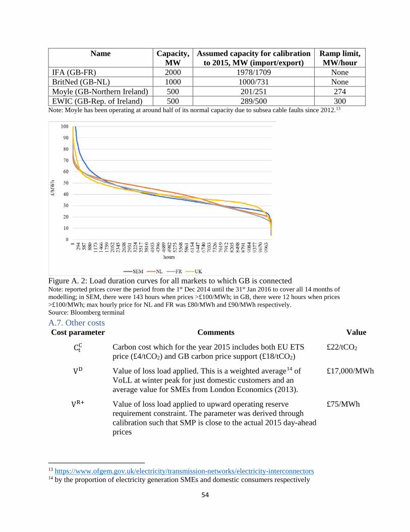
54

Name Capacity, MW

Assumed capacity for calibration to 2015, MW (import/export)

Ramp limit, MW/hour

IFA (GB-FR) 2000 1978/1709 None BritNed (GB-NL) 1000 1000/731 None Moyle (GB-Northern Ireland) 500 201/251 274 EWIC (GB-Rep. of Ireland) 500 289/500 300

Note: Moyle has been operating at around half of its normal capacity due to subsea cable faults since 2012.13

Figure A. 2: Load duration curves for all markets to which GB is connected Note: reported prices cover the period from the 1st Dec 2014 until the 31st Jan 2016 to cover all 14 months of modelling; in SEM, there were 143 hours when prices >£100/MWh; in GB, there were 12 hours when prices >£100/MWh; max hourly price for NL and FR was £80/MWh and £90/MWh respectively. Source: Bloomberg terminal A.7. Other costs Cost parameter Comments Value

CtC Carbon cost which for the year 2015 includes both EU ETS price (£4/tCO2) and GB carbon price support (£18/tCO2)

£22/tCO2

VD Value of loss load applied. This is a weighted average14 of VoLL at winter peak for just domestic customers and an average value for SMEs from London Economics (2013).

£17,000/MWh

VR+ Value of loss load applied to upward operating reserve requirement constraint. The parameter was derived through calibration such that SMP is close to the actual 2015 day-ahead prices

£75/MWh

13 https://www.ofgem.gov.uk/electricity/transmission-networks/electricity-interconnectors 14 by the proportion of electricity generation SMEs and domestic consumers respectively

55

VR− Value of loss load applied to downward operating reserve requirement constraint. The parameter was derived through calibration such that SMP is close to the actual 2015 day-ahead prices

£25/MWh

CCL Cost of curtailing power which is a price of ROC in 2018/19 (Ofgem, 2018)

£47/MWh

CR+ Payment for spinning up reserve availability. The parameter is derived from Locatelli et al. (2015).

£7.66/MW/hour

56

Appendix 2: Detailed modelling results Table A. 9: Coefficient variations of generation, interconnectors and hydro PS under flexibility sensitivities

Flexible case Inflexible case Baseline LP 4_CCGT_Exist_West Burton B 4116% 82% 3899% 6041% 4_CCGT_Exist_Staythorpe 2629% 82% 2508% 82% 5_CCGT_Exist_Sutton Bridge A 1781% 82% 1645% 945% 8_OCGT_Cowes 1535% 82% 1809% 82% 8_OCGT_Indian Queens 1421% 82% 1725% 82% 5_OCGT_Taylors Lane 1403% 82% 1656% 82% 7_CCGT_Exist_Grain (CCGT) 1207% 83% 1226% 1186% 1_CCGT_Exist_Peterhead 655% 85% 720% 597% 5_GT_Baglan Bay GT 569% 82% 911% 882% 4_GT_West Burton A GTs 547% 82% 895% 878% 5_Coal_Aberthaw B 264% 93% 100% 238% 5_Coal_Uskmouth 257% 91% 97% 283% 4_Coal_Ferrybridge C 256% 95% 101% 214% 4_Coal_Ratcliffe-on-Soar 250% 94% 100% 225% 4_Coal_Drax 228% 96% 101% 203% 2_Coal_Longannet 207% 97% 100% 181% 4_Coal_Fiddlers Ferry 165% 97% 99% 169% 4_Coal_West Burton A 158% 98% 98% 159% 5_CCGT_Exist_Corby 158% 94% 463% 227% 5_CCGT_Exist_Rye House 153% 95% 407% 217% 5_CCGT_Exist_Peterborough 147% 95% 392% 213% 4_CCGT_Exist_Deeside 132% 97% 375% 171% 4_Coal_Eggborough 131% 98% 97% 151% 4_CCGT_New_Carrington 128% 97% 340% 164% 5_CCGT_Exist_Little Barford 120% 98% 292% 157% 4_Coal_Cottam 118% 98% 96% 144% 7_CCGT_Exist_Medway 117% 99% 272% 151% 4_Coal_Rugeley B 111% 99% 96% 140% 4_CCGT_Exist_South Humber Bank 108% 100% 235% 141% 5_CCGT_Exist_Shoreham 104% 101% 151% 135% 6_CCGT_Exist_Great Yarmouth 103% 102% 148% 132% 4_CCGT_Exist_Rocksavage 102% 102% 143% 128% 5_CCGT_Exist_Seabank 102% 102% 137% 121% 8_CCGT_Exist_Marchwood 100% 102% 127% 115% 5_CCGT_Exist_Didcot B 99% 101% 121% 107% 5_CCGT_Exist_Coryton 98% 101% 115% 103% 5_CCGT_Exist_Baglan Bay 96% 100% 108% 100%

57

5_CCGT_Exist_Pembroke 95% 99% 102% 94% 5_CCGT_Exist_Barry 93% 97% 95% 92% 7_CCGT_Exist_Damhead Creek 93% 96% 97% 90% 8_CCGT_Exist_Langage 91% 89% 95% 88% 4_CCGT_Exist_Saltend 85% 87% 86% 86% 4_CCGT_Exist_Spalding 85% 87% 85% 85% 5_CCGT_Exist_Severn Power 84% 85% 84% 83% 5_CCGT_Exist_Enfield 83% 84% 83% 82% 4_CCGT_Exist_Brigg 82% 82% 82% 12124% 4_CCGT_Exist_CDCL 82% 82% 82% 3308% 4_CCGT_Exist_Connah's Quay 82% 82% 5507% 12124% 7_Britned_Export 781% 233% 593% 763% 4_East-West_(Wales-Ireland) Export 176% 122% 154% 195% 7_IFA_Export 523% 234% 423% 590% 2_Moyle_Export 180% 126% 159% 201% 7_Britned_Import 86% 117% 88% 86% 4_East-West_(Wales-Ireland) Import 162% 250% 184% 146% 7_IFA_Import 91% 122% 95% 88% 2_Moyle_Import 153% 230% 171% 138% 4_PS_Dinorwig_Charge 465% 274% 408% 1933% 4_PS_Ffestiniog_Charge 371% 282% 337% 1395% 1_PS_Foyers_Charge 318% 238% 300% 1228% 1_PS_Cruachan_Charge 368% 248% 339% 1412% 4_PS_Dinorwig_Discharge 520% 297% 445% 2216% 4_PS_Ffestiniog_Discharge 426% 321% 387% 1692% 1_PS_Foyers_Discharge 368% 278% 350% 1469% 1_PS_Cruachan_Discharge 426% 288% 394% 1670%

Table A. 10: Impact of existing hydro PS on gas and coal generation profit and system operating cost (£ mn/year)

Sensitivity PS profit Gas profit Coal profit

System cost

1 -26.86 -104.67 -731.67 7399.58 2 -3.25 -80.55 -724.18 7418.82 3 -1.22 -97.32 -735.23 7417.91 4 -2.38 -92.47 -729.96 7415.34 5 -35.93 -111.18 -737.64 7396.28 6 -34.75 -135.51 -753.85 7396.33 7 -38.42 -137.33 -754.57 7395.15 8 -5.15 -80.45 -718.19 7412.83

58

9 -7.38 -89.63 -727.04 7409.88 10 -5.93 -107.84 -738.67 7410.81 11 -43.54 -134.05 -753.90 7393.76 12 -47.20 -133.00 -746.68 7392.96 13 -12.38 -112.89 -748.60 7405.30 14 -45.70 -135.02 -747.67 7393.02

Baseline -56.90 -147.84 -753.01 7393.35 Table A. 11: Deriving Shapley value of existing hydro PS for gas generation profitability (£ mn/year)

Changes in profit for gas generation A B C D

(A) 43.17 43.17 0.00 0.00 0.00 (B) 67.30 0.00 67.30 0.00 0.00 (C) 50.52 0.00 0.00 50.52 0.00 (D) 55.38 0.00 0.00 0.00 55.38 (A,B) 36.66 -6.51 -30.64 0.00 0.00 (A,C) 12.33 -30.84 0.00 -38.18 0.00 (A,D) 10.51 -32.66 0.00 0.00 -44.86 (B,C) 67.39 0.00 0.09 16.87 0.00 (B,D) 58.21 0.00 -9.08 0.00 2.84 (C,D) 40.01 0.00 0.00 -10.51 -15.37 (A,B,C) 13.80 -53.59 1.46 -22.86 0.00 (A,B,D) 14.84 -43.37 4.33 0.00 -21.82 (B,C,D) 34.95 0.00 -5.06 -23.27 -32.44 (A,C,D) 12.82 -27.19 0.00 2.31 0.49 (A,B,C,D) 0.00 -34.95 -12.82 -14.84 -13.80

Shapley value, £ mn/year -12.40 1.04 -2.66 -4.64 Note: A – Dinorwig; B – Ffestiniog; C – Foyers; D – Cruachan. Table A. 12: Deriving Shapley value of existing hydro PS for coal generation profitability (£ mn/year)

Changes in profit for coal generation A B C D

(A) 21.34 21.34 0.00 0.00 0.00 (B) 28.83 0.00 28.83 0.00 0.00 (C) 17.78 0.00 0.00 17.78 0.00 (D) 23.05 0.00 0.00 0.00 23.05 (A,B) 15.38 -5.97 -13.45 0.00 0.00 (A,C) -0.84 -22.18 0.00 -18.62 0.00 (A,D) -1.55 -22.90 0.00 0.00 -24.60

59

(B,C) 34.83 0.00 6.00 17.05 0.00 (B,D) 25.97 0.00 -2.86 0.00 2.92 (C,D) 14.34 0.00 0.00 -3.44 -8.71 (A,B,C) -0.89 -35.71 -0.05 -16.27 0.00 (A,B,D) 6.33 -19.64 7.89 0.00 -9.05 (B,C,D) 4.41 0.00 -9.93 -21.56 -30.41 (A,C,D) 5.34 -8.99 0.00 6.90 6.18 (A,B,C,D) 0.00 -4.41 -5.34 -6.33 0.89

Shapley value, £ mn/year -6.56 0.74 -1.63 -2.65 Note: A – Dinorwig; B – Ffestiniog; C – Foyers; D – Cruachan.

Table A. 13: Deriving Shapley value of existing hydro PS for system operating cost (£ mn/year)

Changes in total system cost A B C D

(A) -6.24 -6.24 0.00 0.00 0.00 (B) -25.47 0.00 -25.47 0.00 0.00 (C) -24.57 0.00 0.00 -24.57 0.00 (D) -21.99 0.00 0.00 0.00 -21.99 (A,B) -2.94 3.30 22.53 0.00 0.00 (A,C) -2.99 3.25 0.00 21.58 0.00 (A,D) -1.80 4.43 0.00 0.00 20.19 (B,C) -19.48 0.00 5.99 5.08 0.00 (B,D) -16.53 0.00 8.94 0.00 5.46 (C,D) -17.47 0.00 0.00 7.10 4.52 (A,B,C) -0.41 19.07 2.57 2.52 0.00 (A,B,D) 0.39 16.92 2.19 0.00 3.32 (B,C,D) -11.95 0.00 5.52 4.58 7.53 (A,C,D) 0.32 17.79 0.00 2.12 3.31 (A,B,C,D) 0.00 11.95 -0.32 -0.39 0.41

Shapley value, £ mn/year 4.70 1.46 1.20 1.52 Note: A – Dinorwig; B – Ffestiniog; C – Foyers; D – Cruachan.