energy optimization in wireless sensor networks based on
TRANSCRIPT

Energy Optimization in Wireless Sensor Networks Based on Genetic Algorithms
Angela Rodriguez Intelligent Management Systems University Foundation of Popayán -
FUP Popayán, Colombia
Paolo Falcarin School of Architecture, Computing and Engineering University of East
London London, UK
Armando Ordóñez Intelligent Management Systems University Foundation of Popayán -
FUP Popayán, Colombia
Abstract—Wireless sensor is a consolidated technology with high potential in the Internet of Things. However, some open issues must be tackled in order to leverage the whole potential of this technology. One of the challenges is the energy consumption. Many algorithms have been proposed for saving energy. However these approaches use a mono-objective evaluation and the contradiction between optimization parameters values is not considered. Besides these approaches don’t offer a unique solution. This paper describes MOR4WSN an algorithm based in NSGA-II for selecting the best sensor distribution as well as a mechanism for optimization of results. Experimental evaluation shows promising results in terms of lifetime maximization.
Keywords—wireless sensor networks; genetic algorithm; multi-objective optimization
I. INTRODUCTION
Internet of things (IoT) is based on the pervasive presence of objects or elements such as RFID (Radio frequency identification), sensors, mobile devices, etc. These elements interact with each other in order to reach a common goal [1]. Among this wide set of objects, wireless sensor networks (WSN) play an important role as they allow to collect information from the context which is useful for decision making [1]. Due to advances in sensor technology, these sensors are becoming more and more powerful, economic and smaller. This situation has leveraged deployment of high scale WSN with hierarchy or cluster based topology. One of the main challenges of IoT is energy optimization in each object [2].
Particularly, high scale WSN must afford challenges such as preservation of network longevity. This longevity is reached in part with the reduction of energy consumption due to the fact that sensor have limited energy sources which usually cannot be reloaded once the network is deployed in remote or difficult access areas. While WSN is in operation mode the higher energy consumption is produced during data transmission due to the use of radiofrequency module [1]. Consequently, one of the key factors for optimization of battery lifetime is right selection of paths for information gathering; the latter means to select the best routing topology according to WSN requirements. In this regard, there exist diverse factors that affect battery consumption during data
transmission such as: distance between sensors, network topology, among others. Consequently, this optimization may be seen as a multi objective optimization problem.
Previous approaches [3][4][5][6][7] have used bio inspired techniques such as ant colony optimization or evolutionary techniques like genetic algorithms for defining transmission routes in WSN. However, these works don’t consider multi objective optimization that allows to include diverse factors in the analysis. Besides these approaches don’t offer a unique solution to the optimization problem but a set of solutions. Previously [8] the evolutionary multi-objective algorithm NSGA-II was proposed for optimization of energy consumption in hierarchical WSN. Here, the experimental results of MOR4WSN (Multi-Objective Routing for WSN) algorithm based on NSGA-II are presented. This paper presents the modeling of hierarchical WSN in chromosomes for its use in MOR4 WSN; equally it is presented design and implementation of objective functions for optimization of data gathering paths in hierarchical networks. Experimental results are also presented in this paper.
The rest of this paper is organized as follows: Section 2 presents conceptual background, Section 3 describes the modelling of WSN in genetic algorithms, Section 4 presents the objective functions. Latter Section 5 shows the evaluation of WSN longevity by introducing MOR4WSN in the network. Section 6 describes the related work and finally section 7 details conclusions and future work.
II.BACKGROUND
A. Wireless Sensor Networks
WSN are composed of many sensor nodes known as source nodes which gather data from environment using a sensing module and communicate with other nodes through wireless technologies in order to send data to the central point known as base station or sink node.
As WSN lacks of physical infrastructure, so these WSN can adopt different topologies according to the domain. The most common topology for high scale networks like IoT networks used for city or parks monitoring is the tree or hierarchical topology. Fig. 1 shows a tree WSN rooted with the base station while the rest of the nodes are data sources.
Sponsors: University of Cauca in Colombia and the Administrative Department of Science Technology and Innovation of Colombia – Colciencias.
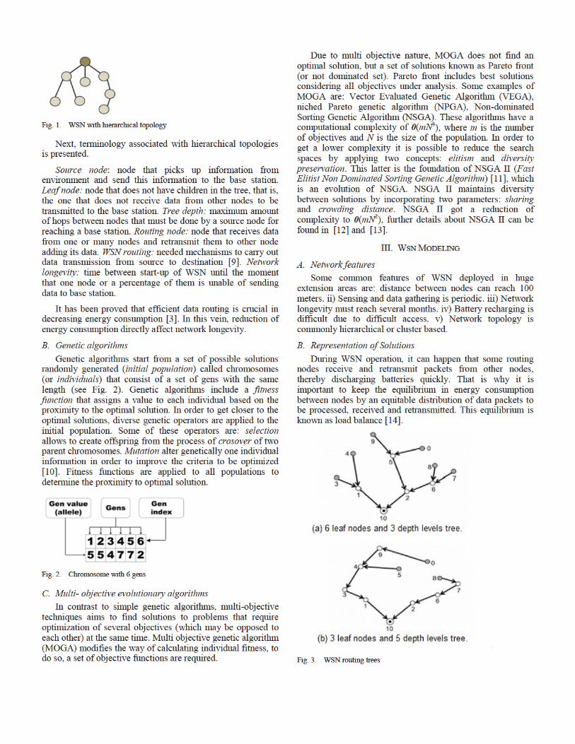
Fig. 1. WSN with hierarchical topology
Next, terminology associated with hierarchical topologies is presented.
Source node: node that picks up information from environment and send this information to the base station. Leaf node: node that does not have children in the tree, that is, the one that does not receive data from other nodes to be transmitted to the base station. Tree depth: maximum amount of hops between nodes that must be done by a source node for reaching a base station. Routing node: node that receives data from one or many nodes and retransmit them to other node adding its data. WSN routing: needed mechanisms to carry out data transmission from source to destination [9]. Network longevity: time between start-up of WSN until the moment that one node or a percentage of them is unable of sending data to base station.
It has been proved that efficient data routing is crucial in decreasing energy consumption [3]. In this vein, reduction of energy consumption directly affect network longevity.
B. Genetic algorithms
Genetic algorithms start from a set of possible solutions randomly generated (initial population) called chromosomes (or individuals) that consist of a set of gens with the same length (see Fig. 2). Genetic algorithms include a fitness function that assigns a value to each individual based on the proximity to the optimal solution. In order to get closer to the optimal solutions, diverse genetic operators are applied to the initial population. Some of these operators are: selection allows to create offspring from the process of crosover of two parent chromosomes. Mutation alter genetically one individual information in order to improve the criteria to be optimized [10]. Fitness functions are applied to all populations to determine the proximity to optimal solution.
Fig. 2. Chromosome with 6 gens
C. Multi- objective evolutionary algorithms
In contrast to simple genetic algorithms, multi-objective techniques aims to find solutions to problems that require optimization of several objectives (which may be opposed to each other) at the same time. Multi objective genetic algorithm (MOGA) modifies the way of calculating individual fitness, to do so, a set of objective functions are required.
Due to multi objective nature, MOGA does not find an optimal solution, but a set of solutions known as Pareto front (or not dominated set). Pareto front includes best solutions considering all objectives under analysis. Some examples of MOGA are: Vector Evaluated Genetic Algorithm (VEGA), niched Pareto genetic algorithm (NPGA), Non-dominated Sorting Genetic Algorithm (NSGA). These algorithms have a computational complexity of 0(mN3), where m is the number of objectives and N is the size of the population. In order to get a lower complexity it is possible to reduce the search spaces by applying two concepts: elitism and diversity preservation. This latter is the foundation of NSGA II (Fast Elitist Non Dominated Sorting Genetic Algorithm) [11], which is an evolution of NSGA. NSGA II maintains diversity between solutions by incorporating two parameters: sharing and crowding distance. NSGA II got a reduction of complexity to 0(mN2), further details about NSGA II can be found in [12] and [13].
III.WSN MODELING
A. Network features
Some common features of WSN deployed in huge extension areas are: distance between nodes can reach 100 meters. ii) Sensing and data gathering is periodic. iii) Network longevity must reach several months. iv) Battery recharging is difficult due to difficult access. v) Network topology is commonly hierarchical or cluster based.
B. Representation of Solutions
During WSN operation, it can happen that some routing nodes receive and retransmit packets from other nodes, thereby discharging batteries quickly. That is why it is important to keep the equilibrium in energy consumption between nodes by an equitable distribution of data packets to be processed, received and retransmitted. This equilibrium is known as load balance [14].
Fig. 3. WSN routing trees
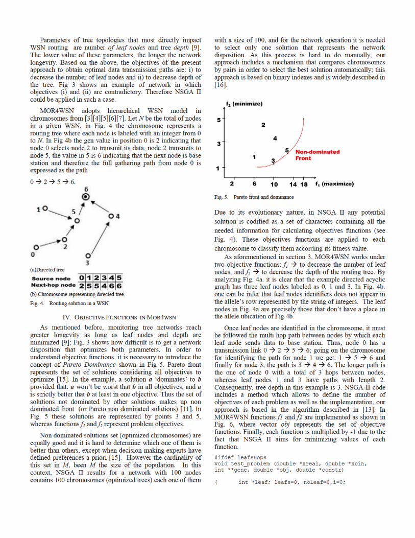
Parameters of tree topologies that most directly impact WSN routing are number of leaf nodes and tree depth [9]. The lower value of these parameters, the longer the network longevity. Based on the above, the objectives of the present approach to obtain optimal data transmission paths are: i) to decrease the number of leaf nodes and ii) to decrease depth of the tree. Fig 3 shows an example of network in which objectives (i) and (ii) are contradictory. Therefore NSGA II could be applied in such a case.
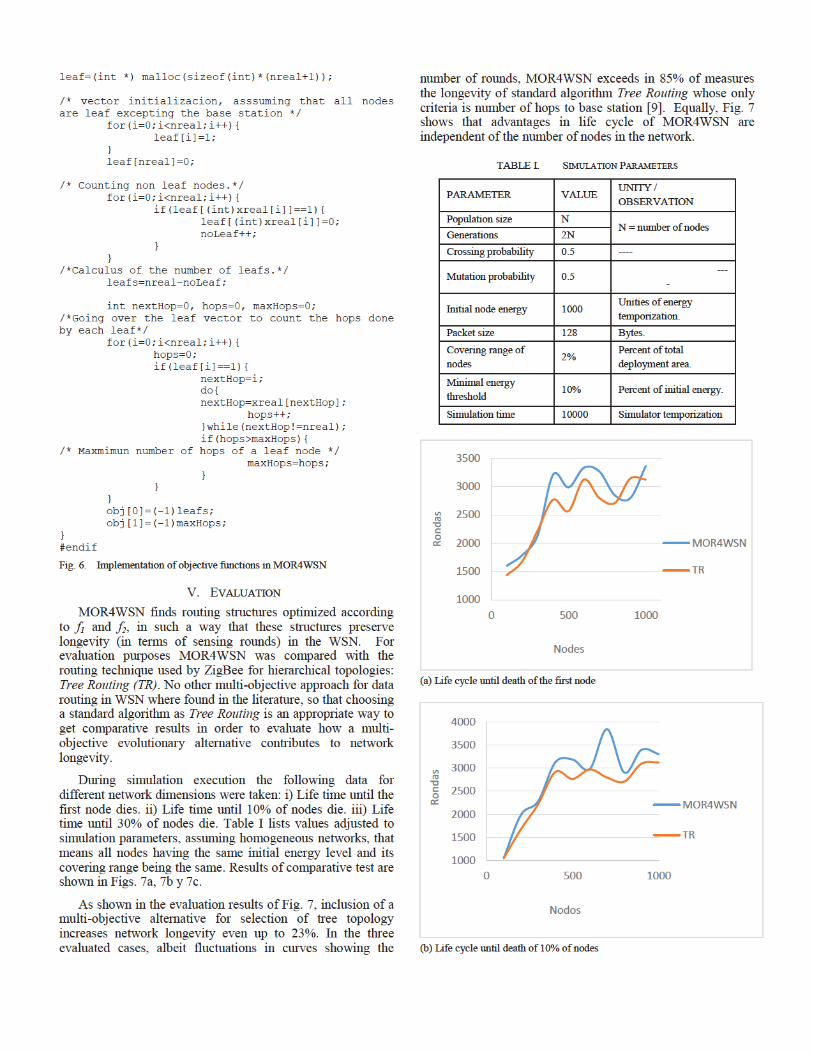
MOR4WSN adopts hierarchical WSN model in chromosomes from [3][4][5][6][7]. Let N be the total of nodes in a given WSN, in Fig. 4 the chromosome represents a routing tree where each node is labeled with an integer from 0 to N. In Fig 4b the gen value in position 0 is 2 indicating that node 0 selects node 2 to transmit its data, node 2 transmits to node 5, the value in 5 is 6 indicating that the next node is base station and therefore the full gathering path from node 0 is expressed as the path
0 2 5 6.
(a)Directed tree
(b) Chromosome representing directed tree.
Fig. 4. Routing solution in a WSN
IV.OBJECTIVE FUNCTIONS IN MOR4WSN
As mentioned before, monitoring tree networks reach greater longevity as long as leaf nodes and depth are minimized [9]; Fig. 3 shows how difficult is to get a network disposition that optimizes both parameters. In order to understand objective functions, it is necessary to introduce the concept of Pareto Dominance shown in Fig 5. Pareto front represents the set of solutions considering all objectives to optimize [15]. In the example, a solution a ‘dominates’ to b provided that: a won’t be worst that b in all objectives, and a is strictly better that b at least in one objective. Thus the set of solutions not dominated by other solutions makes up non dominated front (or Pareto non dominated solutions) [11]. In Fig. 5 these solutions are represented by points 3 and 5, whereas functions f1 and f2 represent problem objectives.
Non dominated solutions set (optimized chromosomes) are equally good and it is hard to determine which one of them is better than others, except when decision making experts have defined preferences a priori [15]. However the cardinality of this set in M, been M the size of the population. In this context, NSGA II results for a network with 100 nodes contains 100 chromosomes (optimized trees) each one of them
with a size of 100, and for the network operation it is needed to select only one solution that represents the network disposition. As this process is hard to do manually, our approach includes a mechanism that compares chromosomes by pairs in order to select the best solution automatically; this approach is based on binary indexes and is widely described in [16].
Fig. 5. Pareto front and dominance
Due to its evolutionary nature, in NSGA II any potential
solution is codified as a set of characters containing all the
needed information for calculating objectives functions (see
Fig. 4). These objectives functions are applied to each
chromosome to classify them according its fitness value.
As aforementioned in section 3, MOR4WSN works under two objective functions: f1 to decrease the number of leaf nodes, and f2 to decrease the depth of the routing tree. By analyzing Fig. 4a. it is clear that the example directed acyclic graph has three leaf nodes labeled as 0, 1 and 3. In Fig. 4b. one can be infer that leaf nodes identifiers does not appear in the allele’s row represented by the string of integers. The leaf nodes in Fig. 4a are precisely those that don’t have a place in the allele ubication of Fig 4b.
Once leaf nodes are identified in the chromosome, it must be followed the multi hop path between nodes by which each leaf node sends data to base station. Thus, node 0 has a transmission link 0 2 5 6; going on the chromosome for identifying the path for node 1 we get: 1 5 6 and finally for node 3, the path is 3 4 6. The longer path is the one of node 0 with a total of 3 hops between nodes, whereas leaf nodes 1 and 3 have paths with length 2. Consequently, tree depth in this example is 3. NSGA-II code includes a method which allows to define the number of objectives of each problem as well as the implementation, our approach is based in the algorithm described in [13]. In MOR4WSN functions f1 and f2 are implemented as shown in Fig. 6, where vector obj represents the set of objective functions. Finally, each function is multiplied by -1 due to the fact that NSGA II aims for minimizing values of each function.
#ifdef leafsHops void test_problem (double *xreal, double *xbin, int **gene, double *obj, double *constr)
{ int *leaf; leafs=0, noLeaf=0,i=0;
leaf=(int *) malloc(sizeof(int)*(nreal+1));
/* vector initializacion, asssuming that all nodes are leaf excepting the base station */
for(i=0;i<nreal;i++){leaf[i]=1;
}leaf[nreal]=0;
/* Counting non leaf nodes.*/ for(i=0;i<nreal;i++){
if(leaf[(int)xreal[i]]==1){leaf[(int)xreal[i]]=0;noLeaf++;
}}
/*Calculus of the number of leafs.*/ leafs=nreal-noLeaf;
int nextHop=0, hops=0, maxHops=0; /*Going over the leaf vector to count the hops done by each leaf*/
for(i=0;i<nreal;i++){hops=0;if(leaf[i]==1){
nextHop=i;do{nextHop=xreal[nextHop];
hops++;}while(nextHop!=nreal);if(hops>maxHops){
/* Maxmimun number of hops of a leaf node */ maxHops=hops;
}}
}obj[0]=(-1)leafs;obj[1]=(-1)maxHops;
} #endif
Fig. 6. Implementation of objective functions in MOR4WSN
V. EVALUATION
MOR4WSN finds routing structures optimized according to f1 and f2, in such a way that these structures preserve longevity (in terms of sensing rounds) in the WSN. For evaluation purposes MOR4WSN was compared with the routing technique used by ZigBee for hierarchical topologies: Tree Routing (TR). No other multi-objective approach for data routing in WSN where found in the literature, so that choosing a standard algorithm as Tree Routing is an appropriate way to get comparative results in order to evaluate how a multi-objective evolutionary alternative contributes to network longevity.
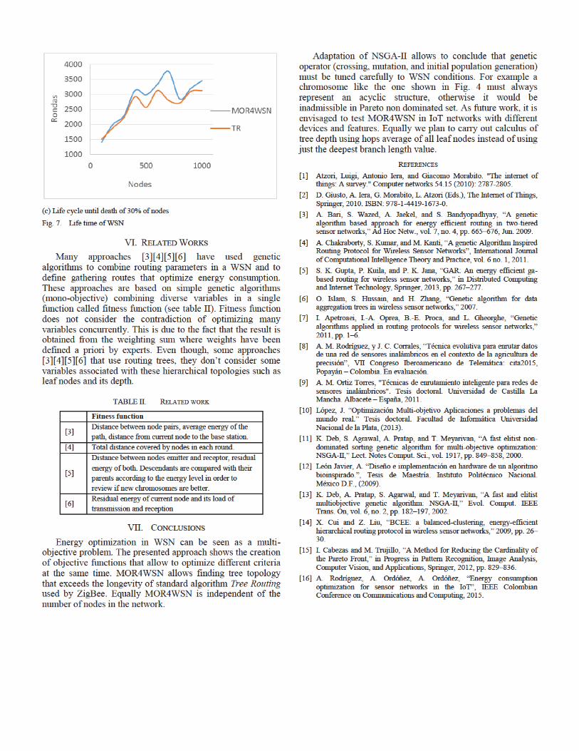
During simulation execution the following data for different network dimensions were taken: i) Life time until the first node dies. ii) Life time until 10% of nodes die. iii) Life time until 30% of nodes die. Table I lists values adjusted to simulation parameters, assuming homogeneous networks, that means all nodes having the same initial energy level and its covering range being the same. Results of comparative test are shown in Figs. 7a, 7b y 7c.
As shown in the evaluation results of Fig. 7, inclusion of a multi-objective alternative for selection of tree topology increases network longevity even up to 23%. In the three evaluated cases, albeit fluctuations in curves showing the
number of rounds, MOR4WSN exceeds in 85% of measures the longevity of standard algorithm Tree Routing whose only criteria is number of hops to base station [9]. Equally, Fig. 7 shows that advantages in life cycle of MOR4WSN are independent of the number of nodes in the network.
TABLE I. SIMULATION PARAMETERS
PARAMETER VALUE UNITY /
OBSERVATION
Population size N N = number of nodes
Generations 2N
Crossing probability 0.5 ----
Mutation probability 0.5 ---
-
Initial node energy 1000 Unities of energy
temporization.
Packet size 128 Bytes.
Covering range of
nodes 2%
Percent of total
deployment area.
Minimal energy
threshold 10% Percent of initial energy.
Simulation time 10000 Simulator temporization
(a) Life cycle until death of the first node
(b) Life cycle until death of 10% of nodes
1000
1500
2000
2500
3000
3500
0 500 1000
Rondas
Nodes
MOR4WSN
TR
1000
1500
2000
2500
3000
3500
4000
0 500 1000
Rondas
Nodos
MOR4WSN
TR
(c) Life cycle until death of 30% of nodes
Fig. 7. Life time of WSN
VI.RELATED WORKS
Many approaches [3][4][5][6] have used genetic algorithms to combine routing parameters in a WSN and to define gathering routes that optimize energy consumption. These approaches are based on simple genetic algorithms (mono-objective) combining diverse variables in a single function called fitness function (see table II). Fitness function does not consider the contradiction of optimizing many variables concurrently. This is due to the fact that the result is obtained from the weighting sum where weights have been defined a priori by experts. Even though, some approaches [3][4][5][6] that use routing trees, they don’t consider some variables associated with these hierarchical topologies such as leaf nodes and its depth.
TABLE II. RELATED WORK
Fitness function
[3] Distance between node pairs, average energy of the
path, distance from current node to the base station.
[4] Total distance covered by nodes in each round.
[5]
Distance between nodes emitter and receptor, residual
energy of both. Descendants are compared with their
parents according to the energy level in order to
review if new chromosomes are better.
[6] Residual energy of current node and its load of
transmission and reception
VII. CONCLUSIONS
Energy optimization in WSN can be seen as a multi-objective problem. The presented approach shows the creation of objective functions that allow to optimize different criteria at the same time. MOR4WSN allows finding tree topology that exceeds the longevity of standard algorithm Tree Routing used by ZigBee. Equally MOR4WSN is independent of the number of nodes in the network.
Adaptation of NSGA-II allows to conclude that genetic operator (crossing, mutation, and initial population generation) must be tuned carefully to WSN conditions. For example a chromosome like the one shown in Fig. 4 must always represent an acyclic structure, otherwise it would be inadmissible in Pareto non dominated set. As future work, it is envisaged to test MOR4WSN in IoT networks with different devices and features. Equally we plan to carry out calculus of tree depth using hops average of all leaf nodes instead of using just the deepest branch length value.
REFERENCES [1] Atzori, Luigi, Antonio Iera, and Giacomo Morabito. "The internet of
things: A survey." Computer networks 54.15 (2010): 2787-2805.
[2] D. Giusto, A. Iera, G. Morabito, L. Atzori (Eds.), The Internet of Things, Springer, 2010. ISBN: 978-1-4419-1673-0.
[3] A. Bari, S. Wazed, A. Jaekel, and S. Bandyopadhyay, “A genetic algorithm based approach for energy efficient routing in two-tiered sensor networks,” Ad Hoc Netw., vol. 7, no. 4, pp. 665–676, Jun. 2009.
[4] A. Chakraborty, S. Kumar, and M. Kanti, “A genetic Algorithm Inspired Routing Protocol for Wireless Sensor Networks”, International Journal of Computational Intelligence Theory and Practice, vol. 6 no. 1, 2011.
[5] S. K. Gupta, P. Kuila, and P. K. Jana, “GAR: An energy efficient ga-based routing for wireless sensor networks,” in Distributed Computing and Internet Technology, Springer, 2013, pp. 267–277.
[6] O. Islam, S. Hussain, and H. Zhang, “Genetic algorithm for data aggregation trees in wireless sensor networks,” 2007.
[7] I. Apetroaei, I.-A. Oprea, B.-E. Proca, and L. Gheorghe, “Genetic algorithms applied in routing protocols for wireless sensor networks,” 2011, pp. 1–6.
[8] A. M. Rodríguez, y J. C. Corrales, “Técnica evolutiva para enrutar datos de una red de sensores inalámbricos en el contexto de la agricultura de precisión”, VII Congreso Iberoamericano de Telemática: cita2015, Popayán – Colombia. En evaluación.
[9] A. M. Ortiz Torres, "Técnicas de enrutamiento inteligente para redes de sensores inalámbricos". Tesis doctoral. Universidad de Castilla La Mancha. Albacete – España, 2011.
[10] López, J. “Optimización Multi-objetivo Aplicaciones a problemas del mundo real.” Tesis doctoral. Facultad de Informática Universidad Nacional de la Plata, (2013).
[11] K. Deb, S. Agrawal, A. Pratap, and T. Meyarivan, “A fast elitist non-dominated sorting genetic algorithm for multi-objective optimization: NSGA-II,” Lect. Notes Comput. Sci., vol. 1917, pp. 849–858, 2000.
[12] León Javier, A. “Diseño e implementación en hardware de un algoritmo bioinspirado.”, Tesis de Maestría. Instituto Politécnico Nacional. México D.F., (2009).
[13] K. Deb, A. Pratap, S. Agarwal, and T. Meyarivan, “A fast and elitist multiobjective genetic algorithm: NSGA-II,” Evol. Comput. IEEE Trans. On, vol. 6, no. 2, pp. 182–197, 2002.
[14] X. Cui and Z. Liu, “BCEE: a balanced-clustering, energy-efficient hierarchical routing protocol in wireless sensor networks,” 2009, pp. 26–30.
[15] I. Cabezas and M. Trujillo, “A Method for Reducing the Cardinality of the Pareto Front,” in Progress in Pattern Recognition, Image Analysis, Computer Vision, and Applications, Springer, 2012, pp. 829–836.
[16] A. Rodríguez, A. Ordóñez, A. Ordóñez, “Energy consumption optimization for sensor networks in the IoT”, IEEE Colombian Conference on Communications and Computing, 2015.