Vilnius University

Faculty of Physics

Laboratory of Atomic and Nuclear Physics

Experiment No. 16

ENERGY LOSS OF ALPHA PARTICLES IN GASES

by Andrius Poškus

(e-mail: andrius.poskus@ff.vu.lt)

2010-02-12

Contents

The aim of the experiment 2

1. Tasks 2

2. Control questions 2

3. The types of ionizing radiation 3

4. Interaction of charged particles with matter 4

4.1. Interaction of heavy charged particles with matter 4 4.2. Interaction of electrons with matter 5 4.3. Mass stopping power 6 4.4. Estimation of particle path in a material from initial and final energies. Particle range 7 4.5. Detector pulse height spectrum 9 4.6. Detector energy resolution 10 4.7. Energy straggling of heavy charged particles 11

5. Experimental setup and procedure 13

5.1. Introduction to the investigation technique 13 5.2. Equipment 17 5.3. Measurement procedure 18

2

The aim of the experiment Measure dependence of alpha particle energy distribution on distance traveled by alpha particles in air and other gases.

1. Tasks 1. Measure the pulse height distribution of the silicon surface barrier detector when the detector is

exposed to radiation of the covered 241Am (americium-241) alpha source placed at 10 cm from the detector, at several values of air pressure (from 10 hPa to 250 hPa). Duration of each measurement should be about 5 min.

2. Measure the pulse height distribution of the detector when the detector is exposed to radiation of the covered 241Am alpha source placed at 10 cm from the detector using four different gases: air, nitrogen (N2), carbon dioxide (CO2) and helium (He) at the same pressure (about 30 to 40 hPa). Duration of each measurement should be about 5 min.

3. Measure the pulse height distribution of the detector when it is exposed to radiation of the open 241Am alpha source placed at 5 to 10 mm from the detector at the lowest achievable pressure.

4. Using the known value of the alpha particles emitted by 241Am and the results of Task 3, calibrate the detector, i. e. determine the ratio of particle energy and average pulse height.

5. For each value of pressure (p) used in Task 1, determine the distance x that an alpha particle has to travel in air at standard pressure (1013 hPa) in order to lose the same amount of energy that it loses after traveling 10 cm at a pressure p.

6. Using the results of Tasks 1, 4 and 5, plot the dependence of average alpha particle energy E on the traveled path x at standard air pressure. Using this dependence, calculate and plot the dependence of the stopping power (−dE/dx) on x.

7. Using the results of Task 6, plot the dependence of the stopping power (−dE/dx) on average energy of alpha particles (E) at standard air pressure.

8. Using the results of Tasks 1, 4 and 5, calculate and plot the dependence of the width of alpha particle energy distribution on the traveled path x at standard air pressure.

9. Using the results of Task 2, calculate the ratio of alpha particle energy decrease to the average number of electrons in a molecule for each gas at equal concentrations of gas molecules.

2. Control questions 1. What are the types of ionizing radiation? 2. What is the origin of energy losses of charged particles in matter? 3. Explain the concept of the stopping power of the medium. What are the main parameters determining

the rate of energy loss? 4. What are the differences between interaction of heavy charged particles (such as alpha particles) with

matter and interaction of electrons with matter? 5. Explain the concept of particle range and its difference from the average penetration depth. 6. Explain the concept of detector pulse height spectrum and its relation to the particle energy spectrum.

Define energy resolution of a detector. Recommended reading: 1. Krane K. S. Introductory Nuclear Physics. New York: John Wiley & Sons, 1988. p. 193 − 198. 2. Lilley J. Nuclear Physics: Principles and Applications. New York: John Wiley & Sons, 2001.

p. 129 − 136. 3. Knoll G. F. Radiation Detection and Measurement. 3rd Edition. New York: John Wiley & Sons, 2000.

p. 30 – 48. 4. Payne M. G. Energy straggling of heavy charged particles in thick absorbers // Physical Review, vol.

185, no. 2, 1969, p. 611 – 623. 5. Laboratory Experiments. Phywe Systeme GmbH, 2005 (compact disc).

3

3. The types of ionizing radiation Ionizing radiation is a flux of subatomic particles (e. g. photons, electrons, positrons, protons,

neutrons, nuclei, etc.) that cause ionization of atoms of the medium through which the particles pass. Ionization means the removal of electrons from atoms of the medium. In order to remove an electron from an atom, a certain amount of energy must be transferred to the atom. According to the law of conservation of energy, this amount of energy is equal to the decrease of kinetic energy of the particle that causes ionization. Therefore, ionization becomes possible only when the energy of incident particles (or of the secondary particles that may appear as a result of interactions of incident particles with matter) exceeds a certain threshold value – the ionization energy of the atom. Ionization energies of isolated atoms are usually of the order of a few electronvolts (eV). 1 eV = 1,6022·10−19 J. The ionization energies of molecules of most gases that are used in radiation detectors are between 10 eV and 25 eV.

Ionizing radiation may be of various nature. The directly ionizing radiation is composed of high-energy charged particles, which ionize atoms of the material due to Coulomb interaction with their electrons. Such particles are, e. g., high-energy electrons and positrons (beta radiation), high-energy 4He nuclei (alpha radiation), various other nuclei. Indirectly ionizing radiation is composed of neutral particles which do not directly ionize atoms or do that very infrequently, but due to interactions of those particles with matter high-energy free charged particles are occasionally emitted. The latter particles directly ionize atoms of the medium. Examples of indirectly ionizing radiation are high-energy photons (ultraviolet, X-ray and gamma radiation) and neutrons of any energy. Particle energies of various types of ionizing radiation are given in the two tables below.

Table 1. The scale of wavelengths of electromagnetic radiation

Spectral region Approximate wavelength range

Approximate range of photon energies

Radio waves 100000 km – 1 mm 1·10−14 eV – 0,001 eV Infrared rays 1 mm – 0,75 μm 0,001 eV – 1,7 eV Visible light 0,75 μm – 0,4 μm 1,7 eV – 3,1 eV

Ionizing electromagnetic radiation: Ultraviolet light 0,4 μm – 10 nm 3,1 eV – 100 eV X-ray radiation 10 nm – 0,001 nm 100 eV – 1 MeV Gamma radiation < 0,1 nm > 10 keV

Table 2. Particle energies corresponding to ionizing radiation composed of particles of matter

Radiation type Approximate range of particle energies

Alpha (α) particles (4He nuclei) 4 MeV – 9 MeV Beta (β) particles (electrons and positrons) 10 keV – 10 MeV Thermal neutrons < 0,4 eV Intermediate neutrons 0,4 eV – 200 keV Fast neutrons > 200 keV Nuclear fragments and recoil nuclei 1 MeV – 100 MeV

The mechanism of interaction of particles with matter depends on the nature of the particles (especially on their mass and electric charge). According to the manner by which particles interact with matter, four distinct groups of particles can be defined: 1) heavy charged particles (such as alpha particles and nuclei), 2) light charged particles (such as electrons and positrons), 3) photons (neutral particles with zero rest mass), 4) neutrons (neutral heavy particles). This experiment concerns only the first mentioned type of particles (heavy charged particles). However, the theoretical background needed for this experiment also includes some information about interaction of light charged particles (specifically, fast electrons) with matter.

4

4. Interaction of charged particles with matter

4.1. Interaction of heavy charged particles with matter In nuclear physics, the term “heavy particles” is applied to particles with mass that is much larger than electron mass (me = 9,1·10−31 kg). Examples of heavy particles are the proton (charge +e, mass mp = 1,67·10−27 kg) and various nuclei (for example, 4He nucleus, which is composed of two protons and two neutrons). When radiation is composed of charged particles, the main quantity characterizing interaction of radiation with matter is the average decrease of particle kinetic energy per unit path length. This quantity is called the stopping power of the medium and is denoted S. An alternative notation is −dE/dx or |dE/dx| (such notation reflects the mathematical meaning of the stopping power: it is opposite to the derivative of particle energy E relative to the traveled path x). The main mechanism of the energy loss of heavy charged particles (and electrons with energies of the order of a few MeV or less) is ionization or excitation of the atoms of matter (excitation is the process when internal energy of the atom increases, but it does not lose any electrons). All such energy losses are collectively called ionization energy losses (this term is applied to energy losses due to excitation, too). Atoms that are excited or ionized due to interaction with a fast charged particle lie close to the trajectory of the incident particle (at a distance of a few nanometers from it). The nature of the interaction that causes ionization or excitation of atoms is the so-called Coulomb force which acts between the incident particles and electrons of the matter. When an incident charged particle passes by an atom, it continuously interacts with the electrons of the atom. For example, if the incident particle has a positive electric charge, it continuously “pulls” the electrons (whose charge is negative) toward itself (see Fig. 1). If the pulling force is sufficiently strong and if its time variation is sufficiently fast (i. e. if the incident particle‘s velocity is sufficiently large), then some of the electrons may by liberated from the atom (i. e., the atom may be ionized). Alternatively, the atom may be excited to higher energy levels without ionization. Coulomb interaction of the incident particles with atomic nuclei is also possible, but it has a much smaller effect on the motion of the incident charged particles, because the nuclei of the material occupy only about 10−15 of the volume of their atoms. Using the laws of conservation of energy and momentum, it can be proved that the largest energy that a non-relativistic particle with mass M can transfer to an electron with mass me is equal to 4meE/M, where E is kinetic energy of the particle. Using the same laws, it can be shown that the largest possible angle between the direction of particle motion after the interaction and its direction prior to the interaction is equal to me / M. Since M exceeds me by three orders of magnitude (see above), we can conclude that the decrease of energy of a heavy charged particle due to a single excitation or ionization event is much smaller than the total kinetic energy of the particle and the incident particle practically does not change its direction of motion when it interacts with an atom (i. e., the trajectories of heavy charged particles in matter are almost straight). Note: The change of the direction of particle motion is called scattering. The quantum mechanical calculation of the mentioned interaction gives the following expression of the stopping power due to ionization energy losses:

22 42e

2 2 20 e

21 ln4π (1 )

mz e nSm I

βε β

⎧ ⎫⎪ ⎪= −⎨ ⎬−⎪ ⎪⎩ ⎭

vv

, (4.1)

where v is the particle velocity, z is its charge in terms of elementary charge e (“elementary charge” e is the absolute value of electron charge), n is the electron concentration in the material, me is electron mass, ε0 is the electric constant (ε0 = 8,854 ⋅ 10-12 F/m), β is the ratio of particle velocity and velocity of light c (i. e. β ≡ v / c), and the parameter I is the mean excitation energy of the atomic electrons (i. e., the mean value of energies needed to cause all possible types of excitation and ionization of the atom). This formula is applicable when v exceeds 107 m/s (this corresponds to alpha particle energy of 2 MeV).

Fig. 1. The classical model of ionization of an atom due to Coulomb interaction of its electrons with an incident heavy charged particle. ze is the electric charge of the incident particle, −e is the electron charge

ze

-e

v

b

x=0

F

F||

5

The strong dependence of the stopping power (4.1) on particle velocity v, its charge z and electron concentration n can be explained as follows. The decrease of particle energy during one interaction is directly proportional to the square of the momentum transferred to the atomic electron (this follows from the general expression of kinetic energy via the momentum). This momentum is proportional to duration of the interaction (this follows from the second Newton’s law), and the latter duration is inversely proportional to v. Therefore the mean decrease of particle energy in one interaction, (and the stopping power) is inversely proportional to v2. The proportionality of the stopping power to z2 follows from the fact that the mentioned momentum transfer is directly proportional to Coulomb force, which is proportional to z according to the Coulomb’s law. The proportionality of the stopping power to n follows from the fact that the mean number of collisions per unit path is proportional to n.

4.2. Interaction of electrons with matter The physical mechanism of ionization energy losses of fast incident electrons as they slow down in matter is similar to that of heavy charged particles. I. e., the incident electron interacts with atomic electrons due to the Coulomb repulsion and either ionizes the atoms or excites them. However, there are some differences, too. First, since the mass of incident electrons is the same as the mass of atomic electrons, even a single collision with an atomic electron can cause a significant change of electron energy and of the direction in which the electron moves (again, this follows from the mentioned laws of conservation of energy and momentum). As a result, an incident electron follows a random erratic path as it slows down in matter. This is the main difference between interaction of fast electrons with matter and interaction of heavy charged particles with matter (as mentioned previously, the path of heavy charged particles in matter is practically straight). Besides, there are additional quantum effects related to the fact that it is impossible to distinguish between the incident electron and the electron that has been removed from an atom due to ionization (these are the so-called “exchange effects”). Taking into account all those effects, the following expression of the stopping power due to ionization energy losses of fast electrons is obtained:

( )224 2 2 2

2 2e2 2 2 20 e e

1 1 1 1 1ln 1 1 ln 2 1 12 2 2 164π 2

m Ee n ESm I m c

β ββ βε

⎧ ⎫⎡ ⎤⎛ ⎞ ⎛ ⎞− −⎪ ⎪⎢ ⎥= + − − − + + − −⎜ ⎟⎨ ⎬⎜ ⎟⎢ ⎥ ⎝ ⎠⎝ ⎠⎪ ⎪⎣ ⎦⎩ ⎭

vv

, (4.2)

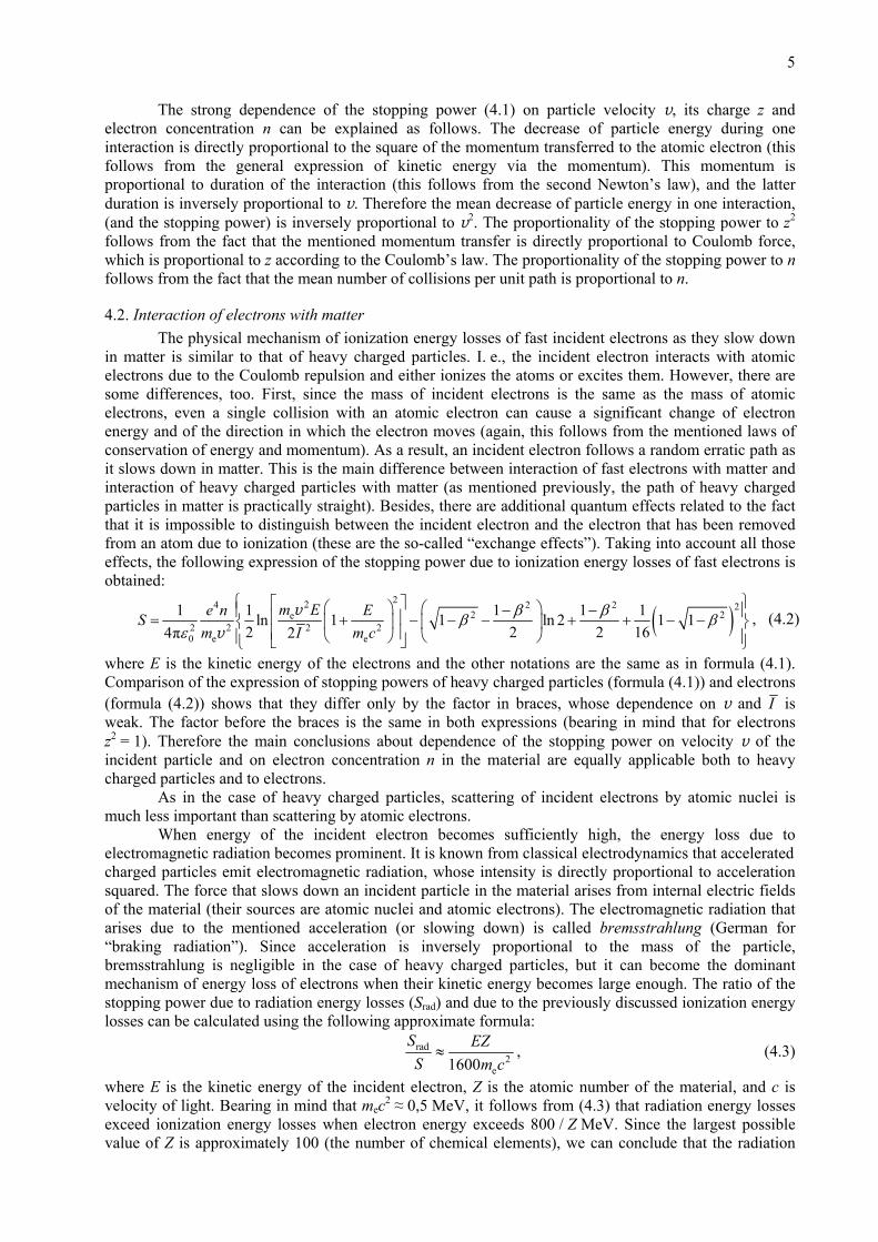
where E is the kinetic energy of the electrons and the other notations are the same as in formula (4.1). Comparison of the expression of stopping powers of heavy charged particles (formula (4.1)) and electrons (formula (4.2)) shows that they differ only by the factor in braces, whose dependence on v and I is weak. The factor before the braces is the same in both expressions (bearing in mind that for electrons z2 = 1). Therefore the main conclusions about dependence of the stopping power on velocity v of the incident particle and on electron concentration n in the material are equally applicable both to heavy charged particles and to electrons. As in the case of heavy charged particles, scattering of incident electrons by atomic nuclei is much less important than scattering by atomic electrons. When energy of the incident electron becomes sufficiently high, the energy loss due to electromagnetic radiation becomes prominent. It is known from classical electrodynamics that accelerated charged particles emit electromagnetic radiation, whose intensity is directly proportional to acceleration squared. The force that slows down an incident particle in the material arises from internal electric fields of the material (their sources are atomic nuclei and atomic electrons). The electromagnetic radiation that arises due to the mentioned acceleration (or slowing down) is called bremsstrahlung (German for “braking radiation”). Since acceleration is inversely proportional to the mass of the particle, bremsstrahlung is negligible in the case of heavy charged particles, but it can become the dominant mechanism of energy loss of electrons when their kinetic energy becomes large enough. The ratio of the stopping power due to radiation energy losses (Srad) and due to the previously discussed ionization energy losses can be calculated using the following approximate formula:

rad2

e1600S EZS m c

≈ , (4.3)

where E is the kinetic energy of the incident electron, Z is the atomic number of the material, and c is velocity of light. Bearing in mind that mec2 ≈ 0,5 MeV, it follows from (4.3) that radiation energy losses exceed ionization energy losses when electron energy exceeds 800 / Z MeV. Since the largest possible value of Z is approximately 100 (the number of chemical elements), we can conclude that the radiation

6

losses are negligible if kinetic energy of the electrons is of the order of a few MeV or less, and then it can be assumed that electrons lose energy only due to ionization energy losses.

4.3. Mass stopping power From the expressions of the stopping power for heavy charged particles (4.1) and electrons (4.2) it follows that the main parameter of the material that determines the magnitude of ionization energy losses of charged particles is electron concentration in the material. If the material is composed of atoms of one chemical element, then

an Zn= , (4.4) where Z is the atomic number of the element (i. e. the number of electrons in one atom), and na the atom concentration in the material. The atom concentration (in cm−3) is equal to ρNA / A, where ρ is density of the material (in g/cm3), NA = 6,022·1023 mol−1 is the Avogadro number and A is the atomic mass of the material (in g/mol). Therefore, electron concentration (in cm−3) is equal to

AZn NA

ρ= . (4.5)

The ratio Z / A varies from 0,5 for light atoms (excluding hydrogen, whose Z / A = 1) to 0,4 for heavy atoms. Thus, ionization energy losses are directly proportional to density of the material ρ, and the coefficient of proportionality is approximately the same in all materials. Summarizing everything that has been said above about ionization energy losses, we can conclude that the ionization stopping power (given by formulas (4.1) and (4.2)) depends on two characteristics of the incident particle – its velocity v and charge z – and on two parameters of the material – its density ρ and the mean atomic excitation energy I (all other quantities in those formulas are principal physical constants). In addition, the quantities z and ρ enter the expression of the stopping power as a multiplicative factor z2ρ, velocity v is uniquely determined by particle kinetic energy E, and dependence on I is logarithmic, i. e. weak. Thus,

2 ( )S z f Eρ≈ ⋅ , (4.6) where f depends only on particle energy. The quantity −dE/(ρdx) ≡ S/ρ is called mass stopping power. From (4.6) it follows that mass stopping power due to ionization energy losses is relatively weakly affected by chemical composition of the material (e. g., see Fig. 2). Therefore, if energy is lost mainly due to atomic ionization and excitation, then the total path of a given particle with a given initial energy (i. e., the length of the path where the particle loses all its kinetic energy, “range”), is mainly determined by density of the material and is inversely proportional to the latter. The expressions of stopping power (4.1), (4.2) and (4.6) do not include the mass of the incident particle. This means that ionization stopping powers of different particles with equal velocity and equal absolute values of electric charge z (for example, electron and proton) are equal. However, stopping powers of electrons and protons with equal energies are very different. This is because velocity of a particle with a given energy is strongly dependent on the particle mass. For example, velocity v and kinetic energy E of a non-relativistic particle are related as follows:

Fig. 2. Dependences of electron mass stopping power in air, aluminum and lead on electron kinetic energy. The solid lines correspond to atomic ionization and excitation, and dashed lines are for radiation (from [1])

0,01 0,1 1,0 10E

MeV

|d /d | / E x ρMeV (g/cm )⋅ 2 1−

0,01

0,1

1,0

10

PbAl

Oras

Pb

Al

Oras

Air

Air

7

2 2EM

=v , (4.7)

where M is the particle mass. After replacing v2 in Eq. (4.1) with the expression (4.7) and taking into account that for non-relativistic particles β << 1, we obtain:

2 4e

2e0

41 ln8π

m Ez e nMSm E IMε

= . (4.8)

We see that ionization energy losses of non-relativistic particles are directly proportional to the mass of the particle. Therefore, ionization stopping power of heavy charged particles (e. g. protons) is much larger than ionization stopping power of electrons with the same energy. For example, the stopping power for 0,5 MeV protons is about 2000 times larger than the stopping power for 0,5 MeV electrons. Hence, a heavy charged particle is able to travel a much smaller distance in a material than an electron with the same energy.

4.4. Estimation of particle path in a material from initial and final energies. Particle range If the dependence of the stopping power S on particle energy E is known, then it is possible to calculate the particle’s path x which corresponds to the decrease of particle energy from the initial value E0 to some smaller value E1. Based on the definition of the stopping power, that path is equal to the integral

0

1

d( )

E

E

ExS E

= ∫ . (4.9)

By replacing S(E) with its expression (4.6), we obtain 0

1

0 12 21 d 1 ( , )

( )

E

E

Ex g E Ef Ez zρ ρ

= ≡∫ , (4.10)

where g(E0, E1) is a universal function of initial and final energies of the particle. Thus, if we know the path x1 that the particle travels in a material, we can easily calculate the equivalent path x2 in a different material, which corresponds to the same decrease of particle energy (from E0 to E1):

12 1

2 2

mxx xρρ ρ

= ≡ , (4.11)

where ρ1 and ρ2 are densities of the two materials, and xm is the so-called “mass path” – the product of the path x and density of the material:

mx xρ≡ . (4.12) The mass path is the mass of a column of matter with height equal to the true path length x and with unit cross-section area (in the above example, the mass path must be equal in both materials). A similar concept to the mass path is the mass thickness dm, which is defined as the product of thickness d of a layer of a material and its density:

md dρ≡ . (4.13) In general, if a particle falls normally to a layer of a material and emerges from its other side, the path travelled inside that layer is different from the layer thickness, because particle’s trajectory inside the layer may not be straight. Since the path is the length of the trajectory (regardless of its shape), the path is in general longer than the thickness. However, since heavy charged particles travel in straight lines, the path of those particles is equal to the layer thickness (assuming that the particles fall normally to its surface). Therefore, in the case of heavy charged particles the path x in the relation (4.11) may be replaced with thickness of the layer of the material d:

12 1

2 2

mdd dρρ ρ

= ≡ . (4.14)

This formula allows calculating thickness d2 of a material 2, such that the particles passing through that layer lose the same amount of energy as they lose passing through a layer of material 1 with thickness d1. The particle range is the total path traveled by the particles in the material until the particle stops. In other words, the range is the total length of the particle’s trajectory. The range can be expressed via the stopping power of the material. That expression is a separate case of a more general relation (4.9), with E1 equal to 0:

8

0

0

d( )

E ERS E

= ∫ , (4.15)

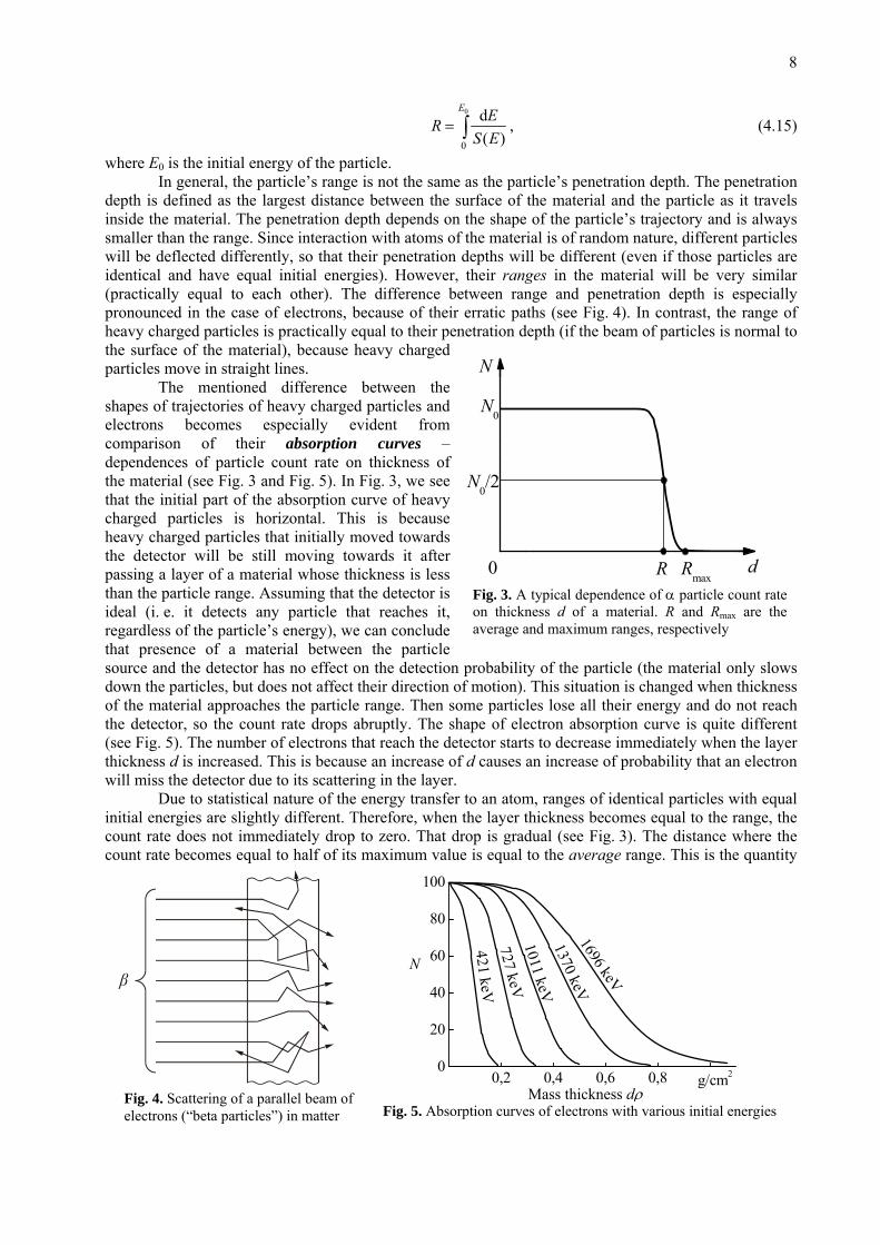
where E0 is the initial energy of the particle. In general, the particle’s range is not the same as the particle’s penetration depth. The penetration depth is defined as the largest distance between the surface of the material and the particle as it travels inside the material. The penetration depth depends on the shape of the particle’s trajectory and is always smaller than the range. Since interaction with atoms of the material is of random nature, different particles will be deflected differently, so that their penetration depths will be different (even if those particles are identical and have equal initial energies). However, their ranges in the material will be very similar (practically equal to each other). The difference between range and penetration depth is especially pronounced in the case of electrons, because of their erratic paths (see Fig. 4). In contrast, the range of heavy charged particles is practically equal to their penetration depth (if the beam of particles is normal to the surface of the material), because heavy charged particles move in straight lines. The mentioned difference between the shapes of trajectories of heavy charged particles and electrons becomes especially evident from comparison of their absorption curves – dependences of particle count rate on thickness of the material (see Fig. 3 and Fig. 5). In Fig. 3, we see that the initial part of the absorption curve of heavy charged particles is horizontal. This is because heavy charged particles that initially moved towards the detector will be still moving towards it after passing a layer of a material whose thickness is less than the particle range. Assuming that the detector is ideal (i. e. it detects any particle that reaches it, regardless of the particle’s energy), we can conclude that presence of a material between the particle source and the detector has no effect on the detection probability of the particle (the material only slows down the particles, but does not affect their direction of motion). This situation is changed when thickness of the material approaches the particle range. Then some particles lose all their energy and do not reach the detector, so the count rate drops abruptly. The shape of electron absorption curve is quite different (see Fig. 5). The number of electrons that reach the detector starts to decrease immediately when the layer thickness d is increased. This is because an increase of d causes an increase of probability that an electron will miss the detector due to its scattering in the layer. Due to statistical nature of the energy transfer to an atom, ranges of identical particles with equal initial energies are slightly different. Therefore, when the layer thickness becomes equal to the range, the count rate does not immediately drop to zero. That drop is gradual (see Fig. 3). The distance where the count rate becomes equal to half of its maximum value is equal to the average range. This is the quantity

Fig. 5. Absorption curves of electrons with various initial energies Fig. 4. Scattering of a parallel beam of electrons (“beta particles”) in matter

β

0,2 0,4 0,6 0,8 1,00

20

40

60

80

100

g/cm2

421 keV727 keV1011 keV1370 keV

1696 keV

N

Masinis storis dρMass thickness dρ

Fig. 3. A typical dependence of α particle count rate on thickness d of a material. R and Rmax are the average and maximum ranges, respectively

RmaxR0

N0/2

N0

d

N

9

that is most frequently used in practice. Further on, we will refer only to the average range, therefore the word “average” will be omitted. If ionization energy losses dominate, then the particle range can be expressed by formula (4.10), where E1 = 0:

0

02 20

1 d 1 ( )( )

E ER Ef Ez z

ϕρ ρ

= ≡∫ , (4.16)

where ϕ(E0) is a universal function of the particle’s initial energy. Thus, if the range R1 of the particle in material 1 is known, than its range R2 in material 2 can be calculated using a simple relation

12 1

2

R Rρρ

= , (4.17)

where ρ1 and ρ2 are densities of the two materials. For this reason, the previously defined concept of range is frequently replaced by the concept of mass range Rm, which is equal to the product of range and material density:

mR Rρ= . (4.18) The mass range of charged particles is approximately the same in all materials. The fact that particle range in a given material is proportional to a universal function of particle initial energy (see Eq. (4.16)) was important in early years of investigation of radioactivity. Having measured the range of α particles in a given material and knowing the function ϕ(E) and density ρ of the material, it is possible to calculate approximate energy of the α particle. Since now there are detectors whose signal height directly reflects particle energy, such indirect methods of energy measurements are

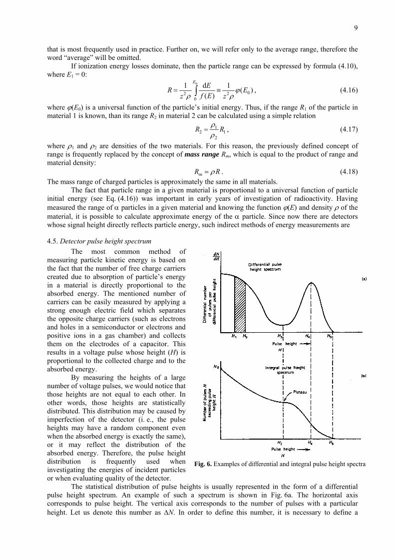
4.5. Detector pulse height spectrum The most common method of measuring particle kinetic energy is based on the fact that the number of free charge carriers created due to absorption of particle’s energy in a material is directly proportional to the absorbed energy. The mentioned number of carriers can be easily measured by applying a strong enough electric field which separates the opposite charge carriers (such as electrons and holes in a semiconductor or electrons and positive ions in a gas chamber) and collects them on the electrodes of a capacitor. This results in a voltage pulse whose height (H) is proportional to the collected charge and to the absorbed energy. By measuring the heights of a large number of voltage pulses, we would notice that those heights are not equal to each other. In other words, those heights are statistically distributed. This distribution may be caused by imperfection of the detector (i. e., the pulse heights may have a random component even when the absorbed energy is exactly the same), or it may reflect the distribution of the absorbed energy. Therefore, the pulse height distribution is frequently used when investigating the energies of incident particles or when evaluating quality of the detector. The statistical distribution of pulse heights is usually represented in the form of a differential pulse height spectrum. An example of such a spectrum is shown in Fig. 6a. The horizontal axis corresponds to pulse height. The vertical axis corresponds to the number of pulses with a particular height. Let us denote this number as ΔN. In order to define this number, it is necessary to define a

Fig. 6. Examples of differential and integral pulse height spectra

10

particular interval of pulse heights. Let us denote the width of this interval as ΔH. Thus, ΔN is the number of pulses with heights between H and H + ΔH. Now, let us take the ratio ΔN / ΔH. If the interval width ΔH is small enough, then the ratio ΔN / ΔH would be the same as the ratio of infinitesimal differences (differentials) dN/dH. The latter ratio is plotted in Fig. 6a. The number of pulses with heights between H1 and H2 can be determined by integrating the differential pulse height spectrum from H1 to H2:

2

1

1 2d( ) dd

H

H

NN H H H HH

< < = ∫ . (4.19)

This integral is shown as a hatched area in Fig. 6a. The total number of pulses is equal to the integral of the entire differential pulse height spectrum:

00

d dd

NN HH

∞

= ∫ . (4.20)

The largest pulse height is given by the abscissa (x-coordinate) of the right edge of the spectrum (for example, in the case of Fig. 6a the largest pulse height is H5). The abscissas of the maxima (peaks) of the spectrum (e. g., H4 in Fig. 6a) correspond to the most probable pulse heights, i. e. such pulse heights that are observed most frequently. The abscissas of the minima of the spectrum (e. g., H3 in Fig. 6a) correspond to least probable pulse heights, i. e., pulse heights that are least likely to be observed. The same information that is contained in a differential pulse height spectrum can be presented in the form of an integral pulse height spectrum. The integral pulse height spectrum gives the total number of pulses with heights greater than a specified value H. In other words, the integral pulse height spectrum is the integral of the differential pulse height spectrum from H to ∞:

d( ) ddH

NN H HH

∞

= ∫ . (4.21)

N(H) is always a decreasing function. The value of the integral pulse height spectrum at H = 0 is equal to the total number of pulses N0. As in the case of the differential pulse height spectrum, the abscissa of the rightmost point of the integral pulse height spectrum is equal to the maximum pulse height (e. g., H5 in Fig. 6b). The differential and integral pulse height spectra are equivalent to each other in terms of the information that they provide. The value of the differential pulse height spectrum corresponding to any value of pulse height H is equal to the absolute value of the slope (i. e. rate of decrease) of the integral spectrum corresponding to the same pulse height. The maxima of the differential spectrum correspond to the largest slope of the integral spectrum (e. g., point H4 in Fig. 6). The minima of the differential spectrum correspond to the smallest slope of the integral spectrum (e. g., point H3 in Fig. 6). In practice, the differential pulse height spectrum is used more frequently than the integral pulse height spectrum, because small changes of the spectrum can be more easily noticed in the differential spectrum than in the integral spectrum.

4.6. Detector energy resolution Radiation detectors are frequently used for measurements of radiation energy spectrum. Such measurements comprise the field of radiation spectroscopy. In this section, we will discuss two related concepts that are important in radiation spectroscopy – energy response function and energy resolution of a detector. Let us assume that energy of all particles that enter the detector is equal to E0. In the ideal case, the heights of all pulses caused by those particles should be also equal to each other and proportional to that E0:

0 0H const E= ⋅ . (4.22) However, as mentioned in Section 4.5, detector pulse heights are not equal to each other even when the incident particles have equal energies. As a result, the relation (4.22) only applies to the average pulse height. I. e., the average pulse height of a real detector is proportional to particle energy. The heights of individual pulses are randomly distributed about the average height. As mentioned, this distribution is usually presented in the form of a differential pulse height spectrum. The differential pulse height spectrum corresponding to a particular energy E0 of incident particles is called the response function of the detector corresponding to particle energy E0. We will denote this function G(H; E0). The pulse height

11

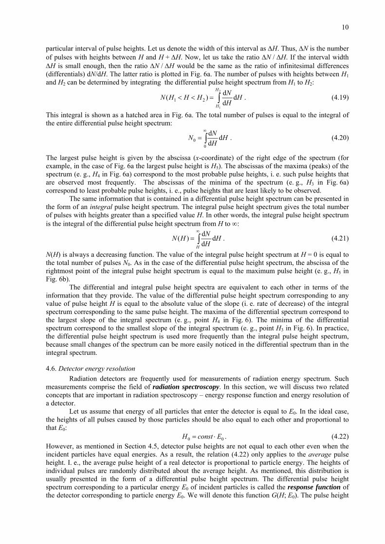
H is the argument of the response function, while the particle energy E0 is its parameter. The shape of the response function is Gaussian:

20 0 0

0 2( ( ))( ; ) exp

22πN H H EG H E

σσ⎛ ⎞−

= −⎜ ⎟⎝ ⎠

, (4.23)

where H0 is the average pulse height (given by (4.22)), σ is the standard deviation of pulse height, and N0 is the total number o pulses (i. e. the integral of the response function from −∞ to +∞). An example of a detector response function is shown in Fig. 7. The statistical uncertainty of pulse height is reflected by the width of the response function. This width (ΔH) is usually measured at half-height of the peak (that is why it is abbreviated FWHM: “full width at half maximum”). If the peak is Gaussian in shape, then FWHM is related to the standard deviation of pulse height as follows:

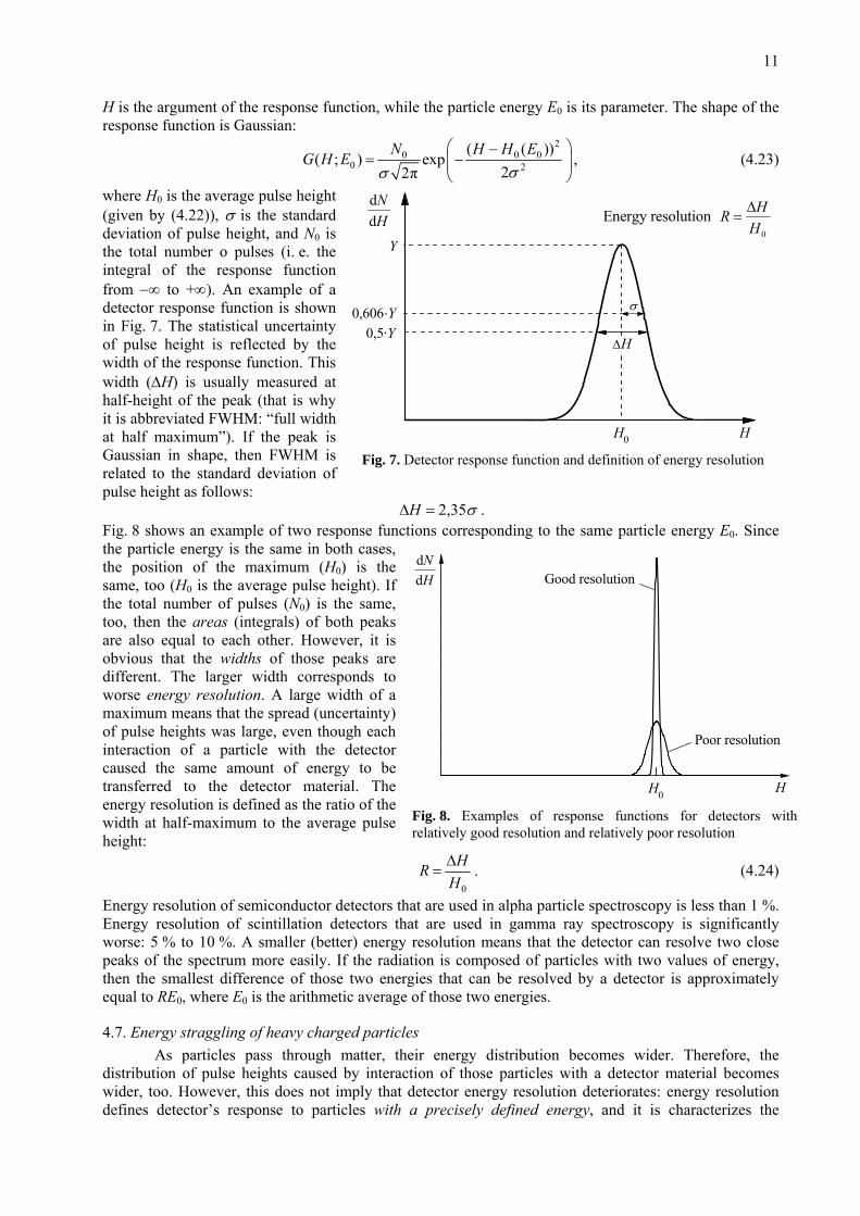
2,35H σΔ = . Fig. 8 shows an example of two response functions corresponding to the same particle energy E0. Since the particle energy is the same in both cases, the position of the maximum (H0) is the same, too (H0 is the average pulse height). If the total number of pulses (N0) is the same, too, then the areas (integrals) of both peaks are also equal to each other. However, it is obvious that the widths of those peaks are different. The larger width corresponds to worse energy resolution. A large width of a maximum means that the spread (uncertainty) of pulse heights was large, even though each interaction of a particle with the detector caused the same amount of energy to be transferred to the detector material. The energy resolution is defined as the ratio of the width at half-maximum to the average pulse height:

0

HRHΔ

= . (4.24)

Energy resolution of semiconductor detectors that are used in alpha particle spectroscopy is less than 1 %. Energy resolution of scintillation detectors that are used in gamma ray spectroscopy is significantly worse: 5 % to 10 %. A smaller (better) energy resolution means that the detector can resolve two close peaks of the spectrum more easily. If the radiation is composed of particles with two values of energy, then the smallest difference of those two energies that can be resolved by a detector is approximately equal to RE0, where E0 is the arithmetic average of those two energies.

4.7. Energy straggling of heavy charged particles As particles pass through matter, their energy distribution becomes wider. Therefore, the distribution of pulse heights caused by interaction of those particles with a detector material becomes wider, too. However, this does not imply that detector energy resolution deteriorates: energy resolution defines detector’s response to particles with a precisely defined energy, and it is characterizes the

Fig. 7. Detector response function and definition of energy resolution

0

Energinė skyra HRHΔ

=Energy resolutiondd

NH

HH0

Y

0,5·Y

ΔH

0,606·Y σ

Fig. 8. Examples of response functions for detectors with relatively good resolution and relatively poor resolution

Poor resolution

dd

NH

HH0

Good resolution

12

detector, not the incident radiation. As mentioned above, detector’s energy resolution is important in situations when it is necessary to resolve two close peaks of the particles’ energy spectrum. In this experiment, the analyzed energy spectrum has a roughly Gaussian shape (as in Fig. 7), and its width is much larger than the width of the detector response function. Under those conditions, the detector’s energy resolution has practically no effect on the shape of the pulse height spectrum. I. e., it may be assumed that the width of the detector’s response function approaches zero (this corresponds to the ideal detector). Then the detector pulse height distribution is determined only by distribution of particle energies. Thus, in this case the width of pulse height distribution can not be used to define energy resolution as in Fig. 7; instead, it defines the fluctuations of particle energies. The widening of particles’ energy distribution as they pass through matter is called energy straggling. The reason of energy straggling is the random nature of a particle’s interaction with an atom of the medium. This randomness means that the amount of energy that the particle loses due to its interaction with an atom of the material is random. This is evident from the model of the interaction described in Section 4.1: the energy transferred to an electron of the atom depends on distance b between the electron and the particle (see Fig. 1), and this distance is a random quantity. The stopping power S (also defined in Section 4.1) defines the rate of decrease of average energy (corresponding to the average pulse height, which is denoted H0 in Fig. 7), but does not provide any information about the change of the width of the energy distribution. In earlier sections, the average energy was denoted E. Now, we will use this notation to denote the exact energy of a particle, whereas the statistical average of the energy will be denoted ⟨E⟩. The average energy ⟨E⟩ depends on distance x that the particles have passed through the medium. If the initial energy of all particles was E0, then their average energy after traveling the distance x in a given material is equal to

00

( ) ( ( ) )dx

E x E S E x x⟨ ⟩ = − ⟨ ⟩∫ , (4.25)

where S(⟨E⟩) is the stopping power (it depends on the average energy). The particles with smaller energy have traveled a larger distance x, therefore they have experienced a larger number of collisions with atoms of the material, therefore their energy has a larger random component. It has been proven theoretically [4] that in the case of relatively large energy decrease (when the decrease E0 − ⟨E⟩ is not much less than the initial energy E0) the energy spectrum of heavy non-relativistic charged particles is roughly Gaussian in shape:

20

2( ( ) )( ; ) exp

2 ( )( ) 2π EE

N E E xf E xxx σσ

⎡ ⎤− ⟨ ⟩= −⎢ ⎥

⎣ ⎦. (4.26)

Interpretation of the energy spectrum f(E; x) is similar to interpretation of the pulse height spectrum defined in Section 4.5. The main difference is that the argument of the energy spectrum is the particle energy E. The distance x is the parameter of the function (4.26), i. e. the quantity that determines the position and width of the Gaussian peak. The area (integral) of the energy spectrum is equal to the total number of particles. The width of the peak at half-maximum is equal to

( ) 2.35 ( )EE x xσΔ = , where σE(x) is the standard deviation of particles’ energy after traveling distance x in the material. It has been shown [4] that when both the initial energy E0 and the average energy ⟨E(x)⟩ of alpha particles are between 1 MeV and 4 MeV, in the case of sufficiently large energy decrease (so that the Gaussian approximation (4.26) is valid) the following approximate expression of the squared standard deviation (variance) of the alpha particle energy can be used:

31.3312 2 e e 0 0

00

2 4 ( )( ) ln 13 ( )Em m E E E xx EM MI E x E

σ− ⎧ ⎫⎡ ⎤⎡ ⎤⎡ ⎤ ⟨ ⟩⎛ ⎞ ⎪ ⎪≈ −⎨ ⎬⎢ ⎥⎢ ⎥⎜ ⎟⎢ ⎥ ⟨ ⟩⎝ ⎠⎣ ⎦ ⎣ ⎦ ⎣ ⎦⎪ ⎪⎩ ⎭

. (4.27)

We can see that both the expression of the stopping power (4.8) and the expression of the energy variance (4.27) include only one parameter that depends on elemental composition of the material (the “elemental composition” is a set of percent quantities equal to the ratio of the number of atoms of each element to the total number of atoms of the material). That parameter is the mean excitation energy I . This quantity is usually determined empirically. One of empirical formulas that relate I to the atomic number of the element is the following:

I ≈ 9.2 · Z + 4.5 · Z1/3 [eV]. (4.28)

13

If the material is composed of several chemical elements, then I can be expressed in terms of the mean excitation energies of constituent elements as follows:

1

K

k kk

I c I=

=∑ , (4.29)

where the sum is over all elements, K is the number of elements in the material, kI is the mean excitation energy of element No. k, and ck is the relative number of atoms of element No. k (i. e. the ratio of the number of atoms of that element to the total number of atoms of the material). For example, if the material is carbon dioxide (CO2), then the relative number of C atoms is 1/3, and the relative number of O atoms is 2/3.

5. Experimental setup and procedure

5.1. Introduction to the investigation technique In this experiment, the energy spectrum of alpha particles is measured. The detector used for those measurements is a semiconductor detector (a silicon surface barrier detector), which generates a voltage pulse each time when an alpha particle strikes its front surface. The energy resolution of that detector is good enough, and the pulse height is proportional to particle energy (see Eq. 4.22), so that it can be assumed that the shape of the detector pulse height spectrum (discussed in Sections 4.5 and 4.6) accurately reflects the shape of the alpha particle energy spectrum (discussed in Section 4.7). The pulse height spectrum is measured using a device called a multichannel analyzer (MCA). It can be described as a number of counters with a common input, with each counter counting only the pulses whose heights belong to a specific narrow interval. This narrow interval of pulse heights is called a channel. Channels are of equal width, they do not overlap and there are no gaps between them. Therefore, when a voltage pulse is applied to the input of the analyzer and when the height of that pulse is between the smallest and largest values that can be measured, that pulse is counted by one (and only one) of the mentioned counters. Thus, the MCA sorts the pulses by their height. After measuring a large enough number of pulses, the pulse height spectrum is obtained. More precisely, the result of measurements is a set of numbers, one number per channel. Each number is the number of pulses whose height belongs to that channel. Let us denote that number δN. Bearing in mind the definition of the pulse height spectrum given in Section 4.5 (as the ratio dN/dH), it may seem that this set of numbers is not exactly the spectrum. However, it may be easily written in the conventional form: δN = δN / δH, where δH = 1. In other words, the channel width δH should be chosen as the unit of pulse height. In order to determine the particle energy spectrum from the pulse height spectrum, the detector has to be calibrated. The aim of calibration is determining the proportionality constant in the relation between particle energy and pulse height (4.22). In order to determine that constant, one has to measure the average pulse height when the detector is exposed to alpha particles of known energy Ecal. Then the energy E of alpha particles that cause pulses of height H can be calculated as follows:

cal

cal

EE HH

= ⋅ . (5.1)

In this experiment, an open 241Am source is used for calibration. Here, the term “open source” means that that the emitted alpha particles do not lose energy in the source cover, hence the energy of alpha particles that reach the detector is equal to the energy of particles emitted from the 241Am nuclei (that energy is equal to 5.486 MeV). However, the 241Am source used for measuring the alpha particle energy loss in gases is covered by a 2 μm-thick foil of gold and palladium alloy, where the alpha particles lose a part of their energy before entering the medium that surrounds the source. This is one of the reasons why the measured energies of alpha particles are significantly smaller than 5.486 MeV and the width of their spectrum is relatively large. Another factor that contributes to decrease of the average energy of alpha particles and to widening of their energy spectrum is the alpha particle energy loss in the gas that separates the source and the detector. In addition to voltage pulses caused by alpha particles, the detector generates a large number of small pulses, which may be caused by external illumination and by thermal noise in the detector electronics. Besides, the 241Am nuclei emit low-energy gamma photons (20 keV and 60 keV), which may also cause small pulses. In the measured pulse height spectra, those small pulses show up as a high peak in the region of small channel numbers (near the left edge of the spectrum). This peak has to be

14

eliminated. This can be achieved by increasing the so-called discrimination level Hd – the smallest pulse height that can be registered by the counting circuit. The same effect can be achieved in a slightly different way: by decreasing the height of all pulses by a constant small amount. Then the heights of the smallest pulses become negative. Those pulses are not registered. The MCA manufactured by the German company “PHYWE Systeme” has a software-controlled parameter “Offset”, which defines the mentioned decrease of pulse height. The increase of this parameter causes a shift of the pulse height spectrum to the left (the part of the spectrum that shifts into the region of negative pulses is eliminated). In the case of the mentioned MCA, at the highest gain, a unit of “Offset” corresponds to 40 channels. I. e., when Offset = 1, the spectrum shifts by 40 channels; when Offset = 2, the spectrum shifts by 80 channels, etc. Accordingly, when the “Offset” parameter is non-zero, Eq. 5.1 has to be modified as follows:

calcal

40 Offset40 Offset

HE EH

+ ⋅= ⋅

+ ⋅, (5.2)

where H and Hcal are channel numbers corresponding to “shifter” spectrum (it is assumed that the “Offset” parameter is the same both for the calibration spectrum and for the investigated spectrum). One of the aims of this experiment is investigation of dependence of alpha particle energy on distance x traveled by the particle in air at standard pressure (1013 hPa). In order to decrease measurement errors and eliminate the need to take into account the change of measurement geometry when x is changed, the measurements are done at a constant distance s between the source and the detector. Instead, air pressure p is varied. The distance x that the particle has to travel in air at standard pressure in order to lose the same amount of energy that it loses after traveling the distance s a pressure p can be determined from the formula

1013 hPapx s= . (5.3)

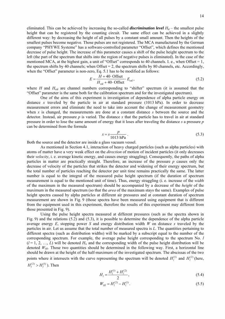
Both the source and the detector are inside a glass vacuum vessel. As mentioned in Section 4.1, interaction of heavy charged particles (such as alpha particles) with atoms of matter have a very weak effect on the direction of motion of incident particles (it only decreases their velocity, i. e. average kinetic energy, and causes energy straggling). Consequently, the paths of alpha particles in matter are practically straight. Therefore, an increase of the pressure p causes only the decrease of velocity of the particles that strikes the detector and widening of their energy spectrum, but the total number of particles reaching the detector per unit time remains practically the same. The latter number is equal to the integral of the measured pulse height spectrum (if the duration of spectrum measurement is equal to the mentioned unit of time). Thus, energy straggling (i. e. increase of the width of the maximum in the measured spectrum) should be accompanied by a decrease of the height of the maximum in the measured spectrum (so that the area of the maximum stays the same). Examples of pulse height spectra caused by alpha particles at different air pressures and at constant duration of spectrum measurement are shown in Fig. 9 (those spectra have been measured using equipment that is different from the equipment used in this experiment, therefore the results of this experiment may different from those presented in Fig. 9). Using the pulse height spectra measured at different pressures (such as the spectra shown in Fig. 9) and the relations (5.2) and (5.3), it is possible to determine the dependence of the alpha particle average energy E, stopping power S and energy distribution width W on distance x traveled by the particles in air. Let us assume that the total number of measured spectra is L. The quantities pertaining to different spectra (such as distribution widths) will be marked by a subscript equal to the number of the corresponding spectrum. For example, the average pulse height corresponding to the spectrum No. l (l = 1, 2, …, L) will be denoted Hl, and the corresponding width of the pulse height distribution will be denoted WHl. Those two quantities should be determined in the following way. First, a horizontal line should be drawn at the height of the half-maximum of the investigated spectrum. The abscissas of the two points where it intersects with the curve representing the spectrum will be denoted (1)

lH and (2)lH (here,

(2) (1)l lH H> ). Then

(1) (2)

2l l

lH HH +

= , (5.4)

(2) (1)Hl l lW H H= − . (5.5)

15

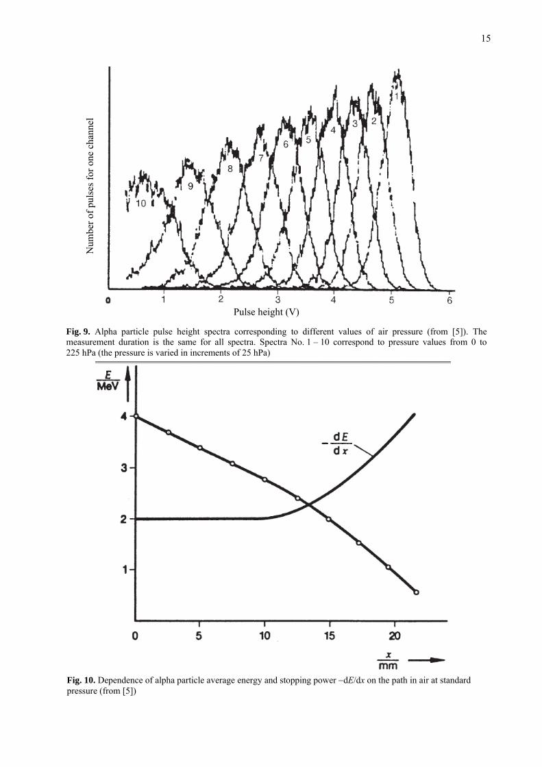
Fig. 10. Dependence of alpha particle average energy and stopping power −dE/dx on the path in air at standard pressure (from [5])

Fig. 9. Alpha particle pulse height spectra corresponding to different values of air pressure (from [5]). The measurement duration is the same for all spectra. Spectra No. 1 – 10 correspond to pressure values from 0 to 225 hPa (the pressure is varied in increments of 25 hPa)

Num

ber o

f pul

ses f

or o

ne c

hann

el

Pulse height (V)

16

The average energy El of alpha particles corresponding to the l-th spectrum is obtained from Eq. 5.2 after replacing H with its expression (5.4). In the same way, we obtain energies (1)

lE and (2)lE corresponding

to values of the spectrum at half-maximum. Thus, the width of the alpha particle energy distribution corresponding to the l-th spectrum is equal to

(2) (1)(2) (1)

calcal 40 Offset

l ll l l

H HW E E EH

−= − = ⋅

+ ⋅. (5.6)

Then it is necessary to calculate the effective distance xl corresponding to each value of pressure pl. If the intervals between adjacent values of xl are small enough, then it can be assumed that dependence E(x) is approximately linear in the interval xl < x < xl+1. In other words, its derivative dE/dx (which is opposite to the stopping power) is approximately constant. The value of the stopping power corresponding to the alpha particle energy (El + El+1) / 2 can be calculated as follows:

1

1 1

12

d2 d l l

l l l lE EE l l

E E E EESx x x+

+ +

+= +

+ −⎛ ⎞ ≡ − ≈⎜ ⎟ −⎝ ⎠. (5.7)

Fig. 10 shows examples of dependences of average energy and stopping power on x calculated in this way. If the gas pressure does not exceed several atmospheres, then the ideal gas law can be applied:

mp n kT= , (5.8) where nm is concentration of gas molecules, k is the Boltzmann constant, and T is the absolute temperature. According to Eq. 5.8, concentration of gas molecules does not depend on the nature of the gas (it only depends on pressure and temperature). However, the expression of the stopping power (4.8) contains not the molecule concentration nm, but electron concentration n, which is equal to the product of molecular concentration nm and the average number of electrons in a molecule ⟨N⟩:

mn n N= ⟨ ⟩ . (5.9) If the gas is composed of J types of molecules, then

1

J

j jj

N c N=

⟨ ⟩ =∑ , (5.10)

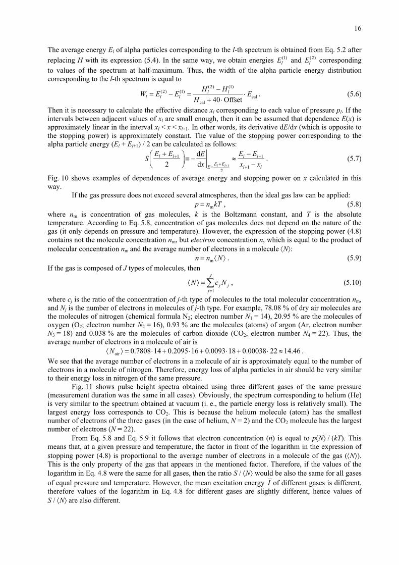
where cj is the ratio of the concentration of j-th type of molecules to the total molecular concentration nm, and Nj is the number of electrons in molecules of j-th type. For example, 78.08 % of dry air molecules are the molecules of nitrogen (chemical formula N2; electron number N1 = 14), 20.95 % are the molecules of oxygen (O2; electron number N2 = 16), 0.93 % are the molecules (atoms) of argon (Ar, electron number N3 = 18) and 0.038 % are the molecules of carbon dioxide (CO2, electron number N4 = 22). Thus, the average number of electrons in a molecule of air is

air 0.7808 14 0.2095 16 0.0093 18 0.00038 22 14.46N⟨ ⟩ = ⋅ + ⋅ + ⋅ + ⋅ ≈ . We see that the average number of electrons in a molecule of air is approximately equal to the number of electrons in a molecule of nitrogen. Therefore, energy loss of alpha particles in air should be very similar to their energy loss in nitrogen of the same pressure. Fig. 11 shows pulse height spectra obtained using three different gases of the same pressure (measurement duration was the same in all cases). Obviously, the spectrum corresponding to helium (He) is very similar to the spectrum obtained at vacuum (i. e., the particle energy loss is relatively small). The largest energy loss corresponds to CO2. This is because the helium molecule (atom) has the smallest number of electrons of the three gases (in the case of helium, N = 2) and the CO2 molecule has the largest number of electrons (N = 22). From Eq. 5.8 and Eq. 5.9 it follows that electron concentration (n) is equal to p⟨N⟩ / (kT). This means that, at a given pressure and temperature, the factor in front of the logarithm in the expression of stopping power (4.8) is proportional to the average number of electrons in a molecule of the gas (⟨N⟩). This is the only property of the gas that appears in the mentioned factor. Therefore, if the values of the logarithm in Eq. 4.8 were the same for all gases, then the ratio S / ⟨N⟩ would be also the same for all gases of equal pressure and temperature. However, the mean excitation energy I of different gases is different, therefore values of the logarithm in Eq. 4.8 for different gases are slightly different, hence values of S / ⟨N⟩ are also different.

17

In this experiment, the composition of the investigated gas is changed by first evacuating the vacuum vessel and then by filling the vessel with the investigated gas. However, since the ideal vacuum can not be achieved, the final composition of the gas includes air, too. This fact must be taken into account when calculating the average electron number in a molecule ⟨N⟩ and the mean excitation energy I . If the residual air pressure is pair and the final pressure (after filling the vessel with the investigated gas) is p, then, after applying equations (5.8) – (5.10), we obtain the following expression of the average electron number in one molecule of the gas that fills the vessel:

air airair g

p p pN N Np p

−⟨ ⟩ = ⟨ ⟩ + , (5.11)

where Ng is number of electrons in one molecule of the investigated pure gas (in this experiment, the investigated pure gases are helium, nitrogen and carbon dioxide).

5.2. Equipment For this experiment, a set of educational equipment manufactured by a German company “Phywe Systeme” is used. The main components of the equipment are the following:

1) alpha detector (semiconductor silicon surface barrier detector), 2) pre-amplifier for the alpha detector, 3) open 241Am source for calibration of the alpha detector (activity 3.7 kBq), 4) covered 241Am source (activity 370 kBq), 5) container for nuclear physics experiments, 6) hand-held mano-/barometer, 7) two-stage diaphragm pump, 8) multichannel analyzer, 9) personal computer, 10) three compressed gas cylinders (helium, nitrogen and CO2), 11) fine control valve.

Fig. 11. Pulse height spectra corresponding to different gases of the same pressure (130 hPa). Measurement duration was the same for all spectra (from [5])

Vacuum N

umbe

r of p

ulse

s for

one

cha

nnel

Pulse height (relative units)

18

The general view of the equipment is shown in Fig. 12. The radioactive source must be screwed to the adjustable source holder, which is at the right-hand side of the glass vessel (the “preparation side”). The detector is at the opposite end of the vessel. The multichannel analyzer has a built-in power supply for the detector. The fine control valve (seen at the end of a rubber hose in Fig. 12) is used for two purposes: it is necessary for attaching a compressed gas cylinder to the glass vessel as shown in Fig. 13 and for slow increase of air pressure during investigation of alpha particle energy loss as a function of air pressure (in the latter case the fine control valve must not be attached to the gas cylinder, as shown in Fig. 12).

Warning: No overpressures are permissible in the vessel in view of the explosion hazard. The three knurled nuts on the preparation side of the vessel should therefore be unscrewed on safety grounds (the cover will remain tightly sealed as long as vacuum is present in the vessel).

5.3. Measurement procedure 1. Connect the equipment as shown in Fig. 12. In the beginning, the multichannel analyzer (MCA)

must be switched off (i. e., no voltage must be applied to the alpha detector). 2. Screw the covered 241Am source to the adjustable source holder. In order to do that, the right-

hand side of the glass vessel must be uncovered by removing three nuts. After that, the vessel cover must be placed back.

Warning: The glass vessel must be handled very carefully in order to avoid cracking. At all times, the vessel must be in horizontal position, firmly placed on the table.

3. Switch on the hand-held mano-/barometer. The arrow at the top of the LCD display of the manometer must be directed to the symbol “Pext”. Otherwise, it must be directed to that symbol using the button „▼“. In this mode, the larger number on the LCD shows the pressure inside the glass vessel and the smaller number shows the ambient pressure. The pressure measurement unit is hectopascal (1 hPa = 100 Pa).

Fig. 12. General view of the measurement equipment

19

4. Close the ventilation screw on the left-hand side of the glass vessel. 5. After checking that the fine control valve is closed, switch on the pump and unscrew the

pinchcock that is on the rubber hose connected to the pump. Wait until the pressure in the glass vessel stops decreasing (if it does not change for more than 2 min, it may be assumed that the lowest pressure has been reached). Then close the rubber hose with the pinchcock and switch off the pump.

6. Set the distance between the covered 241Am source and the detector to 10 cm. 7. Check that the pre-amplifier switch “α/β” is in the position “α”, the switch “Inv” is in the “Off”

position (i. e., in the left position), and the switch “Bias” is in the position “Ext” (then the switch “Bias Int.” may be in any position). The switch “Bias” that is on the MCA must be in the position “−99 V”.

8. Switch on the MCA (the mains switch is on its back panel). 9. Start the program “Measure”.

10. Prepare the program for the measurements, i. e.: a) click the menu command “Gauge/Multi Channel Analyser”, b) select the mode “Spectra recording” and click the button “Continue”, c) in the list box “X-Data”, select the item “Channel number” (this means that the quantity plotted on the X axis is the channel number), d) enter the number “5” in the text field “Interval width [channels]” and press the key “Enter” on the keyboard (then each bar of the graph will correspond to the sum of 5 adjacent channels), e) set the slider “Gain” to the rightmost position, f) enter the number “6” in the text box that is near the slider “Offset” and press the key “Enter” on the keyboard, g) if the check box “Start/Stop” is not checked, then click it, h) click the button “Reset”. Then the program begins measuring the pulse height spectrum.

11. Measure the pulse height spectrum for 5 min. The time should be measured with a precision of 5 s. In order to stop the measurement, click the check box “Start/Stop” (so that it becomes unchecked). Then click the button “Accept data”. Then a new window with the final spectrum opens.

12. Save the graph. This is done by selecting the menu command “Measurement / Export data…”. In the dialog window that pops up, check the boxes “Copy to clipboard” and “Export as metafile”. Then create a Microsoft Word file and paste the graph into it. The graph may be additionally edited by inserting various labels into.

13. Save the measurement data in table format for subsequent analysis. In order to do that, select the menu command “Measurement / Export data…” again, but in this case check the boxes “Save to file” and “Export as numbers”. Then enter the complete file name. Note: In the file, the data will be presented as two columns of numbers. The first column contains channel numbers and the second column contains corresponding numbers of pulses. Since during the measurements each five adjacent channels were merged into a single channel, all channel numbers are multiples of 5.

14. Open carefully the fine control valve and let air flow into the vessel, maintaining constant observation of the manometer. When the pressure inside the vessel increases by approximately 25 hPa, close the fine control valve and repeat Steps 10 to 13. In this way, 9 spectra have to be measured (in each case, the corresponding value of the pressure has to be written down, too). The pressure has to be changed in increments of approximately 25 hPa.

15. Unscrew the three knurled nuts on the right-hand side of the vessel. It is not necessary to remove them completely; it is enough that a gap of about 2 mm is present between each nut and the cover.

16. Ventilate the vessel by unscrewing the ventilation screw on the left-hand side of the vessel.

17. Connect a compressed gas cylinder to the fine control valve (see Fig. 13). At this stage, the fine control valve must be closed. Otherwise, all gas could escape from the gas cylinder and it would be impossible to complete this experiment. Since the fine control valve can be inadvertently opened when connecting the compressed gas cylinder, the

Fig. 13. Connecting the compressed gas cylinder to the fine control valve

20

connection of the compressed gas cylinder must be done by the laboratory supervisor. 18. Close the ventilation screw on the left-hand cover of the glass vessel. 19. Repeat Step 5 (the final pressure should be the same as after Step 5). 20. Open carefully the fine control valve and let the gas flow into the vessel, maintaining constant

observation of the manometer. When the pressure inside the vessel increases by approximately (20 − 60) hPa, close the fine control valve. The final value of the pressure should be equal to one of the values that were obtained in Step 14.

21. Repeat Steps 10 to 13. 22. Ventilate the vessel by unscrewing the ventilation screw on the left-hand side of the vessel. 23. Disconnect the compressed gas cylinder. At this stage, the fine control valve must be closed

(see the explanation in Step 17). Since the fine control valve can be inadvertently opened when disconnecting the compressed gas cylinder, the disconnection of the compressed gas cylinder must be done by the laboratory supervisor.

24. Repeat Steps 17 to 23 with other two compressed gas cylinders (the value of the pressure after completing Step 20 should be the same in all cases).

25. Remove the covered 241Am source and place it into its storage container. Screw the open 241Am source to the source holder. Close the glass vessel (the three knurled nuts on the right-hand cover may be fastened now). Place the source at a distance of about 5 to 10 mm from the detector (the exact value of that distance is not important).

26. a) Close the ventilation screw on the left-hand side of the glass vessel, b) switch on the pump, c) unscrew the pinchcock, d) wait until the pressure inside the vessel stabilizes, e) close the rubber hose with the pinchcock, f) switch off the pump.

27. Repeat Steps 10 to 13. The only change is that measurement duration is not important at this stage; it is sufficient that the total number of pulses exceeds 10000 (the total number of pulses is also shown in the graph window of the program “Measure”).

28. Switch off the MCA, ventilate the glass vessel, open it, remove the open 241Am source from the source holder and put it into its storage container. Cover the glass vessel.

29. Print the measurement data in table format. The tables must only include the channels that correspond to the observed maxima. The tables must be formatted so that they are clear. Each table must have a title and column headers; values of pressure must be included. Various programs may be used for formatting the tables (for example, “Microsoft Word” or “Microsoft Excel”). The list of printers in the “Print” dialog that pops up after selecting the menu command “File/Print” must contain the printer that is present in the laboratory. Notes: 1) The printer that is currently used in the laboratory is not a network printer; instead it is connected to a computer that is connected to LAN. If the system can not establish connection with the printer, this probably means that the mentioned computer or the printer is not switched on. 2) If the mentioned computer and printer are switched on, but there still is an error message after an attempt to print, then open the folder “Computers Near Me” using “Windows Explorer”, locate the computer with name “605-K3-2” and connect to it (user name is “Administrator”, and the password field must be left empty). Then try printing again.

30. Write your name and surname on the printed sheets with measurement results. Show them to the laboratory supervisor for signing. Those sheets will have to be included in the final laboratory report for this experiment.