energy loss analysis of 3d asymmetric trifurcations using cfd

International Journal of Engineering Research & Science (IJOER) ISSN: [2395-6992] [Vol-2, Issue-6 June- 2016]

Page | 129

Energy Loss Analysis of 3D Asymmetric Trifurcations Using CFD Nagappa Pattanashetti

1, Manjunatha S.S

2

1M.Tech Student- Department of Mechanical Engineering, Government Engineering College, Devagiri, Haveri – 581110,

Karnataka, India. Mobile: +91 98 80 112696

[email protected] 2HOD- Department of Mechanical Engineering, Government Engineering College, Devagiri, Haveri – 581110, Karnataka,

India.

[email protected]

Abstract— Head losses are very common in penstock trifurcations. In this paper, six cases of 3D asymmetric trifurcations

have been modeled with main pipe length & diameter of 1.3716m & 0.0254m, respectively and branch pipe lengths &

diameters of 0.762m & 0.0196m, respectively. Volumetric flow rates, velocity magnitudes, dynamic and total pressure

contours and their values have been computed. Energy loss coefficients have been computed for branch pipes for an input air

velocity of 3m/s by pressure data obtained from the CFD analysis. The maximum values of velocity magnitude, dynamic and

total pressures are observed in the branch-2 and head losses in branch-2 are relatively less.

Keywords— Head losses, Energy loss coefficients, 3D asymmetric trifurcations.

I. INTRODUCTION

In penstocks used for hydropower projects, trifurcations along with the other components, help in producing electricity.

These trifurcations supplement water supply to multiple turbines at the same time. Despite having the economical advantage

over independent systems, even this system is not free from losses. The comparison of velocity magnitudes, dynamic and

total pressure contours and determination of head loss coefficients in the branch pipes sums up the interest of this study.

II. DOMAIN

A total of six cases have been modeled using Gambit 2.4.6, with each model displaying an asymmetry about the central

branch axis. The dimensions used for the six cases in the current analysis are shown in the table 1.

TABLE 1

DIMENSIONS OF ASYMMETRIC TRIFURCATIONS

Dimensions In Meter

Length of Main Pipe (L) 1.3716

Diameter of Main Pipe (D) 0.0254

Lengths of branch pipes (l1, l2, l3) 0.762

Diameters of branch pipes (d1, d2, d3) 0.0196

The angle between the branch-2 and branch-1 is termed “α” and the angle between the branch-2 and branch-3 is termed “β”.

The angles used for the six cases are shown in the table 2.

TABLE 2

ANGLES “α” AND “β” FOR THE SIX CASES

Case No. 1 2 3 4 5 6

Angle “α” in Degrees 5 10 15 10 15 20

Angle “β” in Degrees 10 15 20 5 10 15

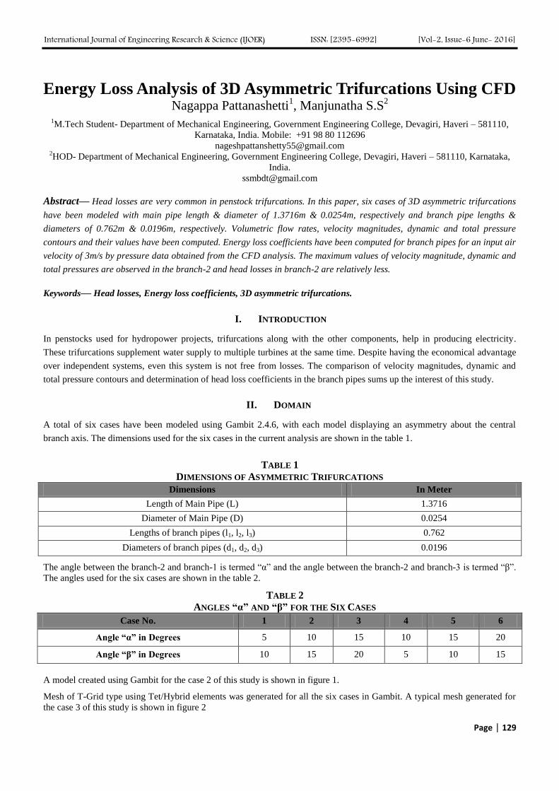
A model created using Gambit for the case 2 of this study is shown in figure 1.

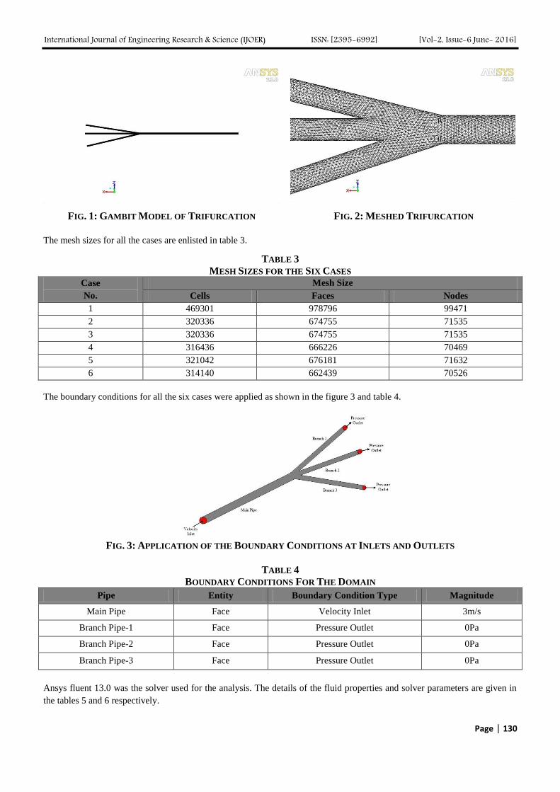
Mesh of T-Grid type using Tet/Hybrid elements was generated for all the six cases in Gambit. A typical mesh generated for

the case 3 of this study is shown in figure 2

mailto:[email protected]

mailto:[email protected]


Page | 130

FIG. 1: GAMBIT MODEL OF TRIFURCATION FIG. 2: MESHED TRIFURCATION

The mesh sizes for all the cases are enlisted in table 3.

TABLE 3

MESH SIZES FOR THE SIX CASES

Case

No.

Mesh Size

Cells Faces Nodes

1 469301 978796 99471

2 320336 674755 71535

3 320336 674755 71535

4 316436 666226 70469

5 321042 676181 71632

6 314140 662439 70526

The boundary conditions for all the six cases were applied as shown in the figure 3 and table 4.

FIG. 3: APPLICATION OF THE BOUNDARY CONDITIONS AT INLETS AND OUTLETS

TABLE 4

BOUNDARY CONDITIONS FOR THE DOMAIN

Pipe Entity Boundary Condition Type Magnitude

Main Pipe Face Velocity Inlet 3m/s

Branch Pipe-1 Face Pressure Outlet 0Pa



Ansys fluent 13.0 was the solver used for the analysis. The details of the fluid properties and solver parameters are given in

the tables 5 and 6 respectively.


Page | 131

TABLE 5

FLUID PROPERTIES

Fluid Fluid Properties

Density Viscosity

Air 1.225kg/m3 1.7874 × 10

-5 kg/m-s

TABLE 6

SOLVER PARAMETERS, INITIALISATION AND CALCULATION DETAILS

Pressure-Velocity Coupling Simple

Spatial Discretization

Gradient Least Square Cells Based

Pressure Second Order

Momentum Second Order Upwind

Solution Initialization Initialisation Methods Standard Initialisation

Reference Frames Relative to Cell Zone

No. of Iterations 1000

The analysis has been carried out for the six cases under the following assumptions:

No slip condition; which means that the relative velocity of the fluid at the solid boundaries is zero.

The fluid flow is incompressible.

Air is a Newtonian fluid.

Steady flow occurs.

III. VOLUMETRIC FLOW RATES, VELOCITIES AND DYNAMIC & TOTAL PRESSURE VALUES

The values of velocity magnitudes, dynamic and total pressures have been obtained for the branched flow as well as inlet for

the surface areas of all the six cases from fluent. These values are tabulated in the tables 7-12.

TABLE 7

VOLUMETRIC FLOW RATES, VELOCITY MAGNITUDES, DYNAMIC AND TOTAL PRESSURES FOR CASE 1

Surface Area Volumetric Flow Rate

(m3/s)

Velocity Magnitude

(m/s)

Dynamic Pressure

(Pa)

Total Pressure

(Pa)

Inlet 1.5 × 10-3

3 5.3621 15.7877

Branch Pipe-1 4.32 × 10-4

1.44 1.4374 1.4466


2.32 3.6253 3.6428


1.28 1.1392 1.1464

TABLE 8



(m3/s)

Velocity Magnitude

(m/s)

Dynamic Pressure

(Pa)

Total Pressure

(Pa)

Inlet 1.5 × 10-3

3 5.3892 16.0206


1.47 1.4711 1.4851


2.36 3.6804 3.7145


1.21 1.0035 1.0092

TABLE 9



(m3/s)

Velocity Magnitude

(m/s)

Dynamic Pressure

(Pa)

Total Pressure

(Pa)

Inlet 1.5 × 10-3

3 5.3957 16.2117


1.41 1.3503 1.3603


2.35 3.6775 3.7062


1.29 1.1277 1.1363


Page | 132

TABLE 10



(m3/s)

Velocity Magnitude

(m/s)

Dynamic Pressure

(Pa)

Total Pressure

(Pa)

Inlet 1.5 × 10-3

3 5.3956 15.7296


1.21 1.0018 1.0100


2.23 3.3027 3.3298


1.61 1.7367 1.7520

TABLE 11



(m3/s)

Velocity Magnitude

(m/s)

Dynamic Pressure

(Pa)

Total Pressure

(Pa)

Inlet 1.5 × 10-3

3 5.3892 16.0252


1.29 1.1389 1.1488


2.31 3.5319 3.5633


1.45 1.4160 1.4296

TABLE 12



(m3/s)

Velocity Magnitude

(m/s)

Dynamic Pressure

(Pa)

Total Pressure

(Pa)

Inlet 1.5 × 10-3

3 5.3890 16.2039


1.33 1.1957 1.2054


2.3 3.4997 3.5283


1.42 1.3707 1.3799

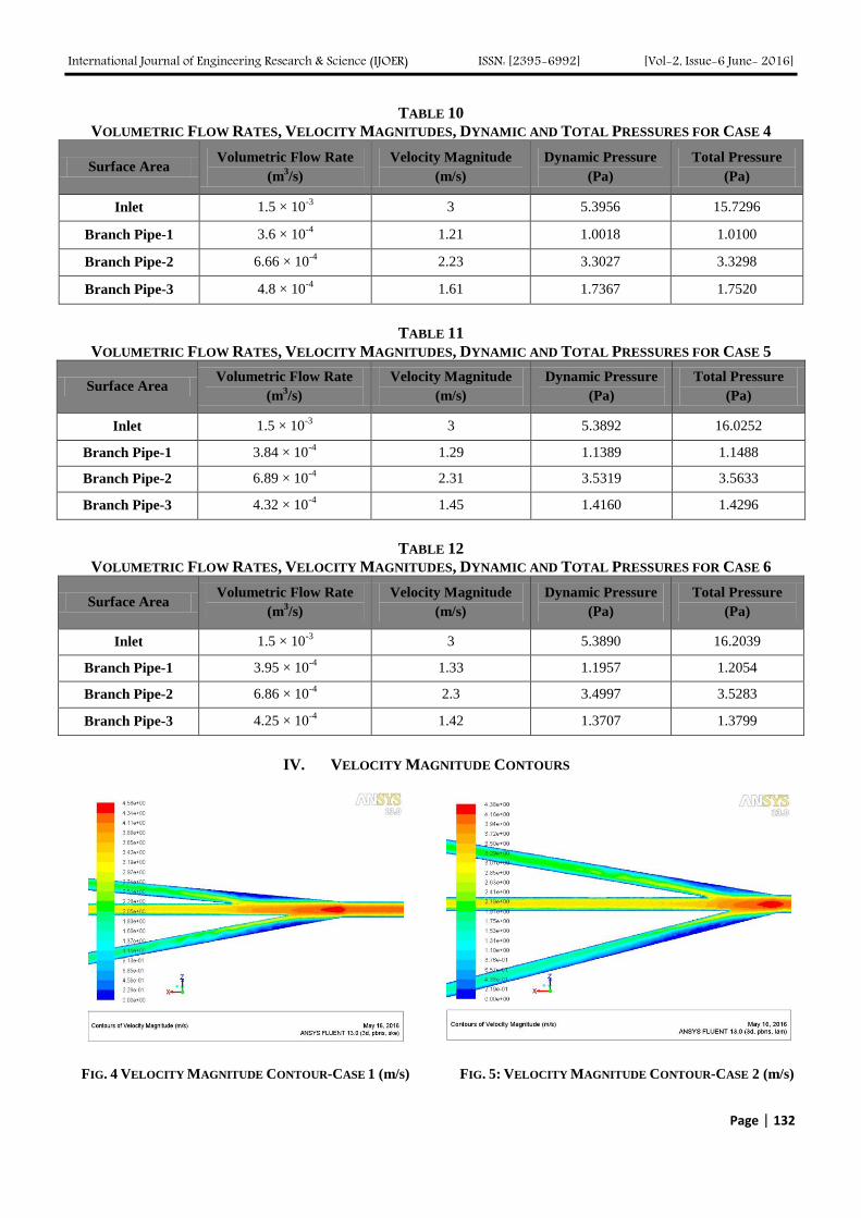
IV. VELOCITY MAGNITUDE CONTOURS

FIG. 4 VELOCITY MAGNITUDE CONTOUR-CASE 1 (m/s) FIG. 5: VELOCITY MAGNITUDE CONTOUR-CASE 2 (m/s)


Page | 133

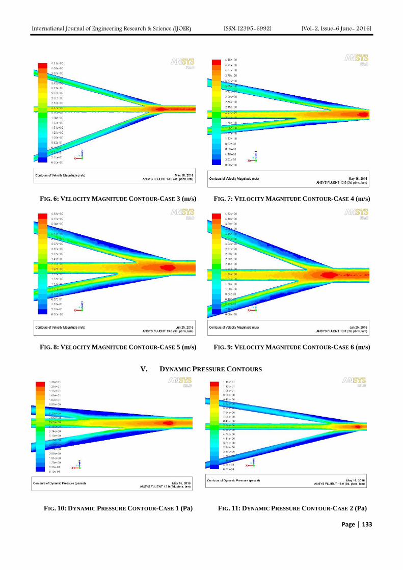
FIG. 6: VELOCITY MAGNITUDE CONTOUR-CASE 3 (m/s) FIG. 7: VELOCITY MAGNITUDE CONTOUR-CASE 4 (m/s)

FIG. 8: VELOCITY MAGNITUDE CONTOUR-CASE 5 (m/s) FIG. 9: VELOCITY MAGNITUDE CONTOUR-CASE 6 (m/s)

V. DYNAMIC PRESSURE CONTOURS

FIG. 10: DYNAMIC PRESSURE CONTOUR-CASE 1 (Pa) FIG. 11: DYNAMIC PRESSURE CONTOUR-CASE 2 (Pa)


Page | 134



VI. TOTAL PRESSURE CONTOURS

FIG. 16: TOTAL PRESSURE CONTOUR-CASE 1 (Pa) FIG. 17: TOTAL PRESSURE CONTOUR-CASE 2 (Pa)


Page | 135



VII. CALCULATION OF HEAD LOSS COEFFICIENTS

The head losses in the individual branches can be calculated using the following formula [1]:

(1)

Where;

PT 1, 2, 3 Total Pressure in branches 1, 2 and 3

PT Inlet Total Pressure in Inlet Pipe

VT Inlet Reference flow velocity at Inlet

ρ Density of air

The velocity magnitudes and pressure values obtained from the fluent analysis are used to carry out the calculations of head

losses for all the branches of each trifurcation case. The reference inlet flow velocity (VInlet = 3 m/s) [2] and density of air (ρ

= 1.225 kg/m3) are constant for all the calculations.

The head loss coefficients have been calculated and their values have been tabulated in the table XII.


Page | 136

The above formula yields negative values of head loss coefficients for all the branches of trifurcations. However, the non-

dimensional coefficients (k) can be called energy change coefficients rather than head loss coefficients whenever branching

of flows occurs [3]. Thus, the negative sign can be ignored here and head loss coefficients can be considered as energy loss

coefficients.

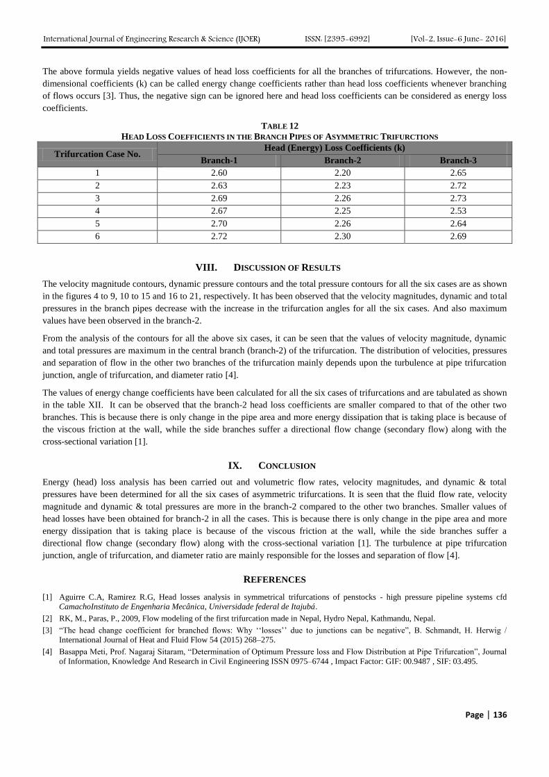
TABLE 12

HEAD LOSS COEFFICIENTS IN THE BRANCH PIPES OF ASYMMETRIC TRIFURCTIONS

Trifurcation Case No. Head (Energy) Loss Coefficients (k)

Branch-1 Branch-2 Branch-3

1 2.60 2.20 2.65

2 2.63 2.23 2.72

3 2.69 2.26 2.73

4 2.67 2.25 2.53

5 2.70 2.26 2.64

6 2.72 2.30 2.69

VIII. DISCUSSION OF RESULTS

The velocity magnitude contours, dynamic pressure contours and the total pressure contours for all the six cases are as shown

in the figures 4 to 9, 10 to 15 and 16 to 21, respectively. It has been observed that the velocity magnitudes, dynamic and total

pressures in the branch pipes decrease with the increase in the trifurcation angles for all the six cases. And also maximum

values have been observed in the branch-2.

From the analysis of the contours for all the above six cases, it can be seen that the values of velocity magnitude, dynamic

and total pressures are maximum in the central branch (branch-2) of the trifurcation. The distribution of velocities, pressures

and separation of flow in the other two branches of the trifurcation mainly depends upon the turbulence at pipe trifurcation

junction, angle of trifurcation, and diameter ratio [4].

The values of energy change coefficients have been calculated for all the six cases of trifurcations and are tabulated as shown

in the table XII. It can be observed that the branch-2 head loss coefficients are smaller compared to that of the other two

branches. This is because there is only change in the pipe area and more energy dissipation that is taking place is because of

the viscous friction at the wall, while the side branches suffer a directional flow change (secondary flow) along with the

cross-sectional variation [1].

IX. CONCLUSION

Energy (head) loss analysis has been carried out and volumetric flow rates, velocity magnitudes, and dynamic & total

pressures have been determined for all the six cases of asymmetric trifurcations. It is seen that the fluid flow rate, velocity

magnitude and dynamic & total pressures are more in the branch-2 compared to the other two branches. Smaller values of

head losses have been obtained for branch-2 in all the cases. This is because there is only change in the pipe area and more

energy dissipation that is taking place is because of the viscous friction at the wall, while the side branches suffer a

directional flow change (secondary flow) along with the cross-sectional variation [1]. The turbulence at pipe trifurcation

junction, angle of trifurcation, and diameter ratio are mainly responsible for the losses and separation of flow [4].

REFERENCES

[1] Aguirre C.A, Ramirez R.G, Head losses analysis in symmetrical trifurcations of penstocks - high pressure pipeline systems cfd

CamachoInstituto de Engenharia Mecânica, Universidade federal de Itajubá.

[2] RK, M., Paras, P., 2009, Flow modeling of the first trifurcation made in Nepal, Hydro Nepal, Kathmandu, Nepal.

[3] “The head change coefficient for branched flows: Why „„losses‟‟ due to junctions can be negative”, B. Schmandt, H. Herwig /

International Journal of Heat and Fluid Flow 54 (2015) 268–275.

[4] Basappa Meti, Prof. Nagaraj Sitaram, “Determination of Optimum Pressure loss and Flow Distribution at Pipe Trifurcation”, Journal

of Information, Knowledge And Research in Civil Engineering ISSN 0975–6744 , Impact Factor: GIF: 00.9487 , SIF: 03.495.

energy loss analysis of 3d asymmetric trifurcations using cfd

Documents