energy integration opportunities in zero emission lng re
TRANSCRIPT
Product Design and ManufacturingJune 2011Truls Gundersen, EPTÅse Slagtern, Aker Solutions
Submission date:Supervisor:Co-supervisor:
Norwegian University of Science and TechnologyDepartment of Energy and Process Engineering
Energy Integration Opportunities inZero Emission LNG Re-Gasification
Katrine Willa Hjertnes

Preface
Preface

Preface

Preface

Preface
I
Preface
This master thesis is written by Katrine Willa Hjertnes at NTNU, Department of Energy and
Process Engineering, and is an extension of the project work from fall 2010. The thesis is
provided by Aker Solutions, Norway.
Firstly I would like to thank Aker Solutions for an interesting and challenging project. I will
also express my gratitude to my supervisors Truls Gundersen and Hans Kristian Rusten for
support with material, answering questions and giving great guidance throughout the project.
In addition I would like to thank my fellow student Mia Skrataas for proofreading, and PhD
student Fu Chao for technical advises regarding the air separation unit.
Special thanks are addressed to my co-habitants; Marthe Aalvik, Ruth Helene Kyte and Adele
M. Slotsvik. Finally, I would like to thank my wonderful family; Hilde M. Hjertnes, Ketil
Nesse and Petter Hjertnes for their patience, support and love through five years of studies. I
could not have done this without you.
June 27th
2011, Trondheim
Katrine Willa Hjertnes

Summary
II
Summary
III
Summary
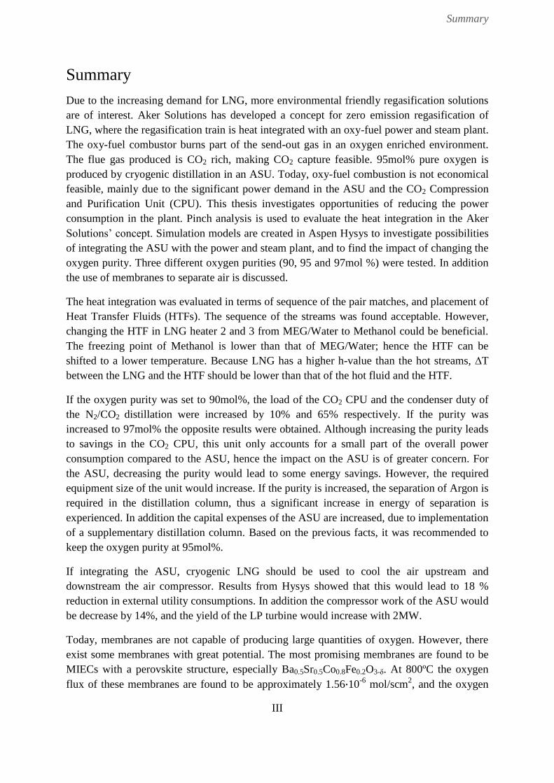
Due to the increasing demand for LNG, more environmental friendly regasification solutions
are of interest. Aker Solutions has developed a concept for zero emission regasification of
LNG, where the regasification train is heat integrated with an oxy-fuel power and steam plant.
The oxy-fuel combustor burns part of the send-out gas in an oxygen enriched environment.
The flue gas produced is CO2 rich, making CO2 capture feasible. 95mol% pure oxygen is
produced by cryogenic distillation in an ASU. Today, oxy-fuel combustion is not economical
feasible, mainly due to the significant power demand in the ASU and the CO2 Compression
and Purification Unit (CPU). This thesis investigates opportunities of reducing the power
consumption in the plant. Pinch analysis is used to evaluate the heat integration in the Aker
Solutions’ concept. Simulation models are created in Aspen Hysys to investigate possibilities
of integrating the ASU with the power and steam plant, and to find the impact of changing the
oxygen purity. Three different oxygen purities (90, 95 and 97mol %) were tested. In addition
the use of membranes to separate air is discussed.
The heat integration was evaluated in terms of sequence of the pair matches, and placement of
Heat Transfer Fluids (HTFs). The sequence of the streams was found acceptable. However,
changing the HTF in LNG heater 2 and 3 from MEG/Water to Methanol could be beneficial.
The freezing point of Methanol is lower than that of MEG/Water; hence the HTF can be
shifted to a lower temperature. Because LNG has a higher h-value than the hot streams, ∆T
between the LNG and the HTF should be lower than that of the hot fluid and the HTF.
If the oxygen purity was set to 90mol%, the load of the CO2 CPU and the condenser duty of
the N2/CO2 distillation were increased by 10% and 65% respectively. If the purity was
increased to 97mol% the opposite results were obtained. Although increasing the purity leads
to savings in the CO2 CPU, this unit only accounts for a small part of the overall power
consumption compared to the ASU, hence the impact on the ASU is of greater concern. For
the ASU, decreasing the purity would lead to some energy savings. However, the required
equipment size of the unit would increase. If the purity is increased, the separation of Argon is
required in the distillation column, thus a significant increase in energy of separation is
experienced. In addition the capital expenses of the ASU are increased, due to implementation
of a supplementary distillation column. Based on the previous facts, it was recommended to
keep the oxygen purity at 95mol%.
If integrating the ASU, cryogenic LNG should be used to cool the air upstream and
downstream the air compressor. Results from Hysys showed that this would lead to 18 %
reduction in external utility consumptions. In addition the compressor work of the ASU would
be decrease by 14%, and the yield of the LP turbine would increase with 2MW.
Today, membranes are not capable of producing large quantities of oxygen. However, there
exist some membranes with great potential. The most promising membranes are found to be
MIECs with a perovskite structure, especially Ba0.5Sr0.5Co0.8Fe0.2O3-δ. At 800ºC the oxygen
flux of these membranes are found to be approximately 1.56∙10-6
mol/scm2, and the oxygen

Summary
IV
purity obtained is above 99mol%. The thickness of one of these membrane were found to be
1.8mm, hence more than 1∙109 membranes are required to produce enough oxygen for the
oxy-combustion plant. Although these membranes have a great potential, they need to be
further evolved before implemented to oxy-fuel power plants.

Sammendrag
V
Sammendrag
Grunnet en økende etterspørsel etter LNG, har interessen for å finne mer miljøvennlige
regasifiseringsteknologier økt. AKSO har utviklet et konsept der LNG regasifiseres med svært
lave utslipp. Regasifiseringsenheten er varmeintegrert med et kraft- og dampanlegg, der deler
av den produserte naturgassen brennes i et oksygen rikt miljø. Dette fører til en CO2-rik
eksosgass, og muliggjør CO2 fangst. Kryogenisk luftseparasjon er brukt til å produsere
95mol % ren oksygen. AKSO sitt konsept er ikke en konkurransedyktig teknologi idag.
Hovedgrunnen er at både luftseparasjonen og CO2 fangsten har et høyt kraftforbruk. Denne
masteroppgaven ser på muligheter for å senke kraftforbruket ved å evaluere
varmeintegrasjonen i anlegget. I tillegg vil muligheter for varmeintegrasjon av
luftseparasjonsenheten bli vurdert, og innvirkningen av å øke eller senke oksygenrenhenheten.
Implementering av membraner for luftseparasjon er også diskutert. Aspen Hysys er brukt som
simuleringsverktøy i denne masteroppgaven.
Varmeintegrasjonen i anlegget er vurdert på følgende vilkår; rekkefølge av strømmer som
varmeveksles, og plassering av mellomliggende medier. Rekkefølgen på strømmene som
varmveksles ble funnet akseptabel. I LNG varmeveksler 2-3 viste undersøkelser at det kan
være gunstig å bruke Metanol isteden for MEG/Vann, som mellomliggende mediet. Dette er
grunnet det lave frysepunktet til Metanol, som fører til at det mellomliggende mediet kan
plasseres nærmere den kalde strømmen.
Systemet ble testet for to forskjellige oksygenrenheter; 90 mol % og 97 mol %. Resultatene
viser at kompressor arbeidet, nedstrøms brenneren, vil øke noe (10 %) hvis renheten ble
senket. Derimot vil kjølebehovet i N2/CO2 destillasjonskolonnen øke betydelig; 65 %. Hvis
oksygen renheten derimot økes til 97mol % vil det motsatte skje, kjølebehovet synker med
65 %, og kompressorarbeidet med 10 %. Selv om økning av oksygenrenheten fører til
reduksjon i kraftbehovet for CO2 renseanlegget, vil denne reduksjonen være liten sett i
forhold til økning av kraftbehovet i luftseparasjonsenheten. For luftseparasjonsenheten vil
separasjonsenergien i destillasjonskolonnen minke med noen få prosent når oksygenrenheten
senkes. Derimot vil størrelsen på produksjonsutstyret øke betydelig. Hvis oksygenrenheten
derimot økes vil økningen i separasjonsenergi være signifikant. Dette er fordi argon da må
separeres fra oksygenet. I tillegg vil kapitalkostnadene øke da implementeringen av en ekstra
kolonne er nødvendig. Det er derfor anbefalt å ikke endre oksygenrenheten i systemet.
Luftseparasjonsenheten ble varmeintegrert med LNG regasifiseringsenheten ved å
varmeveksle LNG mot luft før og etter luftkompressoren. Dette førte til 18 % reduksjon i
dampforbruk. I tillegg ble kompressorarbeidet i luftseparasjonsenheten redusert med 14 %, og
2 MW mer kraft ble produsert i lavtrykksturbinen.
Idag finnes det ingen membraner som kan produserer store kvantum oksygen, men det finnes
noen membraner med stort potensial; ion - elektron ledende membraner. En av de mest
lovende membranene er Ba0.5Sr0.5Co0.8Fe0.2O3-δ. Oksygen fluksen gjennom disse membranene

Sammendrag
VI
er 1.56 10-6
mol/scm2
ved 800 ºC, og de kan produsere oksygen med 99 mol % renhet. Disse
membranene er 1.8 mm tykk, og det kreves derfor over 1 109 membraner for å produsere nok
oksygen til kraftverket. Selv om membranene har stort potensial må de videreutvikles før de
kan tas i bruk i store kraftanlegg.
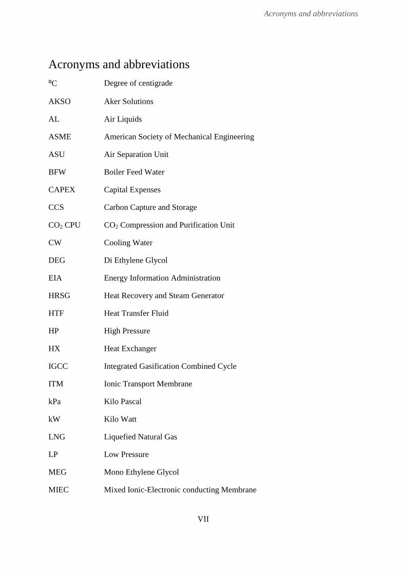
Acronyms and abbreviations
VII
Acronyms and abbreviations
⁰C Degree of centigrade
AKSO Aker Solutions
AL Air Liquids
ASME American Society of Mechanical Engineering
ASU Air Separation Unit
BFW Boiler Feed Water
CAPEX Capital Expenses
CCS Carbon Capture and Storage
CO2 CPU CO2 Compression and Purification Unit
CW Cooling Water
DEG Di Ethylene Glycol
EIA Energy Information Administration
HRSG Heat Recovery and Steam Generator
HTF Heat Transfer Fluid
HP High Pressure
HX Heat Exchanger
IGCC Integrated Gasification Combined Cycle
ITM Ionic Transport Membrane
kPa Kilo Pascal
kW Kilo Watt
LNG Liquefied Natural Gas
LP Low Pressure
MEG Mono Ethylene Glycol
MIEC Mixed Ionic-Electronic conducting Membrane

Acronyms and abbreviations
VIII
MP Medium Pressure
MW Mega Watt
NG Natural Gas
NGCC Natural Gas Combined Cycle
OPEX Operating Expenses
ORV Open Rack Vaporizer
PC Pulverized Coal
ppm Parts per million
SCV Submerged Combustion Vaporizer
SRK Soave-Redlich-Kwong
TEG Tri Ethylene Glycol
WEG Water Ethylene Glycol

Nomenclature
IX
Nomenclature
A Speed of sound [m/s]
A Area [m2]
AF Air-Fuel ratio [kg Air/kg Fuel]
Cp Heat capacity at constant pressure [kg/kgK]
Cv Heat capacity at constant volume [kg/kgK]
Dij Mass diffusivity [m2/s]
F Faradays constant [C/mol]
F Feed [kmol/h]
H Specific enthalpy [kJ/kg]
H Film heat transfer coefficient [W/m2K]
K Isentropic index [ - ]
L Length [m]
L Liquid [kmol/h]
M Molecular weight [kg/kmol]
M Mass [kg]
m Mass flow [kg/s]
N Charge [C]
N Polytrophic index [ - ]
N Amount of moles [mole]
P Pressure [kPa]
PM Permeability [m3(STP)/m
2bar h]
Q Heat flow [kW]
R Ideal gas constant [kJ/kmolK]
Rf Thermal resistance [K/W]

Nomenclature
X
S Solubility [m3 solute(STP)/m
3 solid atm]
T Temperature [K] [C]
U Overall heat transfer coefficient [W/m2K]
V Volume [m3]
V Vapor [kmol/h]
V Specific volume [m3/kg]
W Work [kW]
X Molar fraction in liquid phase [mol%]
Y Molar fraction in vapor phase [mol%]
Z Compressibility factor [ - ]
Chemical symbols
Ba Barium
CH4 Methane
C2H6 Ethane
C3H8 Propane
CO Carbon monoxide
Co Cobalt
CO2 Carbon dioxide
Fe Iron
Gd Gadolinium
H2O Water
N2 Nitrogen
NOx Nitrogen oxides
O2 Oxygen
O3 Ozone

Nomenclature
XI
Sr Strontium
Zn Sink
Greek letters
Α Relative volatility [ - ]
∆ Mean difference [ - ]
Σ Ionic conductivity [S/m]
Η Efficiency [ - ]
Subscript
C Cold stream
H Hot stream
I Component i of a gas
J Component j of a gas
` Denotes the state of the gas at
the feed side
`` Denotes the state of the gas at
the permeate side

Table of Contents
XII

Table of Contents
XIII
Table of Contents
Preface ......................................................................................................................................... I
Summary .................................................................................................................................. III
Sammendrag .............................................................................................................................. V
Acronyms and abbreviations ................................................................................................... VII
Nomenclature ........................................................................................................................... IX
Table of Contents .................................................................................................................. XIII
List of figures ....................................................................................................................... XVII
List of tables ....................................................................................................................... XVIII
1 Introduction ........................................................................................................................ 1
1.1 Background .................................................................................................................. 2
1.2 Thesis structure and limitations ................................................................................... 2
2 Introduction to Aker Solutions regasification concept ....................................................... 5
2.1 Regasification unit ....................................................................................................... 5
2.2 Oxy – fuel steam and power system ............................................................................ 6
2.3 Air separation unit ....................................................................................................... 7
2.4 CO2 compression and purification unit ....................................................................... 7
2.5 Overall plant performance ........................................................................................... 8
3 CO2 Capture and storage .................................................................................................... 9
3.1 CO2 capture by oxy-fuel combustion .......................................................................... 9
3.2 CO2 Compression and purification ............................................................................ 10
3.2.1 Fundamentals of compression ............................................................................ 10
3.2.2 CO2 CPU design ................................................................................................. 11
3.3 Available oxy-fuel configurations ............................................................................. 13
3.3.1 Oxy-fuel NGCC ................................................................................................. 14
3.3.2 Oxy-fuel burner .................................................................................................. 14

Table of Contents
XIV
4 Air separation technology ................................................................................................ 17
4.1 Distillation ................................................................................................................. 17
4.2 Cryogenic air separation unit ..................................................................................... 18
5 Possibilities of power reduction ....................................................................................... 21
5.1 Integration between an ASU and an oxy-fuel power cycle ....................................... 21
5.2 Impact of changing the oxygen purity ....................................................................... 22
5.2.1 Impact on the ASU ............................................................................................. 22
5.2.2 Impact on the CO2 CPU ..................................................................................... 23
6 Membranes used for air separation .................................................................................. 25
6.1 Introduction ............................................................................................................... 25
6.2 Inorganic membranes for air separation .................................................................... 25
6.2.1 Transportation mechanism of inorganic membranes ......................................... 26
6.2.2 Structure of MIECs ............................................................................................ 27
6.2.3 Performance of MIECs ....................................................................................... 28
6.3 Implementation of membranes in oxy-fuel systems .................................................. 30
6.3.1 ITMs used for oxygen production today ............................................................ 30
6.3.2 MIECs integrated with an oxy-fuel plant ........................................................... 30
7 Fundamentals of heat integration ..................................................................................... 33
7.1 Composite and grand composite curves .................................................................... 33
7.2 Steam generation ....................................................................................................... 35
7.3 Intermediate Heat Carriers ......................................................................................... 36
7.4 Heat transfer coefficient ............................................................................................ 37
7.5 Area targeting ............................................................................................................ 39
8 Simulation model and methodology ................................................................................ 41
8.1 Simulation software ................................................................................................... 41
8.2 Fluid packages ........................................................................................................... 41

Table of Contents
XV
8.2.1 Distillation column in Hysys .............................................................................. 41
8.3 Process design and methodology ............................................................................... 42
8.3.1 Specifications of the LNG stream ...................................................................... 43
8.3.2 Specifications of the steam cycle ....................................................................... 44
8.3.3 Specifications of the reactor ............................................................................... 45
8.3.4 Specifications of the CO2 recovery process ....................................................... 45
8.4 Results and discussion ............................................................................................... 47
8.4.1 LNG stream ........................................................................................................ 47
8.4.2 Steam cycle ........................................................................................................ 48
8.4.3 CO2 CPU ............................................................................................................ 49
8.4.4 Power and heat balance ...................................................................................... 52
9 Evaluation of existing heat integration in the system ...................................................... 53
9.1 Methodology .............................................................................................................. 53
9.2 Data extraction ........................................................................................................... 53
9.2.1 Steam cycle ........................................................................................................ 53
9.2.2 LNG and flue gas streams .................................................................................. 55
9.3 Results and discussion ............................................................................................... 57
9.3.1 Composite curves for the system ....................................................................... 57
9.3.2 Sequence of the streams ..................................................................................... 57
9.4 Placement of HTFs .................................................................................................... 61
9.4.1 Placement of HTF in LNG HX 1 ....................................................................... 62
9.4.2 Placement of HTF in LNG HX 2 and LNG HX3 .............................................. 63
10 Different oxygen purities ................................................................................................. 65
10.1 Case studies ............................................................................................................ 65
10.2 Result and discussion ............................................................................................. 66
10.2.1 Flue gas composition .......................................................................................... 66

Table of Contents
XVI
10.2.2 Compressor work of the CO2 CPU and the ASU ............................................... 67
10.2.3 Energy of separation in the CO2 CPU and the ASU .......................................... 69
11 Possibilities of integrating the ASU ................................................................................. 71
11.1 Methodology .......................................................................................................... 71
11.1.1 Simulation models .............................................................................................. 72
11.2 Results and discussion ........................................................................................... 73
12 Proposed system ............................................................................................................... 75
12.1 Chosen parameters and assumptions ..................................................................... 75
12.1.1 Selected oxygen purity ....................................................................................... 75
12.1.2 Selected heat integration scheme ....................................................................... 75
12.2 Proposed system configuration .............................................................................. 75
12.3 Possibility of using ITMs for oxygen production .................................................. 77
12.4 Possible configuration of the system ..................................................................... 77
12.5 Impact on the CO2 CPU ......................................................................................... 78
13 Conclusion and further work ............................................................................................ 79
13.1 Conclusion ............................................................................................................. 79
13.2 Further work ........................................................................................................... 79
List of References ..................................................................................................................... 81
Appendices ............................................................................................................................... 85
Appendix A ............................................................................................................................. i
Appendix B ............................................................................................................................ v
Appendix C ........................................................................................................................... vi
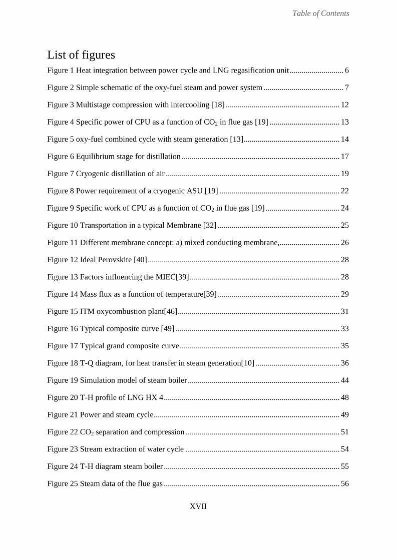
Table of Contents
XVII
List of figures
Figure 1 Heat integration between power cycle and LNG regasification unit ........................... 6
Figure 2 Simple schematic of the oxy-fuel steam and power system ........................................ 7
Figure 3 Multistage compression with intercooling [18] ......................................................... 12
Figure 4 Specific power of CPU as a function of CO2 in flue gas [19] ................................... 13
Figure 5 oxy-fuel combined cycle with steam generation [13] ................................................ 14
Figure 6 Equilibrium stage for distillation ............................................................................... 17
Figure 7 Cryogenic distillation of air ....................................................................................... 19
Figure 8 Power requirement of a cryogenic ASU [19] ............................................................ 22
Figure 9 Specific work of CPU as a function of CO2 in flue gas [19] ..................................... 24
Figure 10 Transportation in a typical Membrane [32] ............................................................. 25
Figure 11 Different membrane concept: a) mixed conducting membrane, .............................. 26
Figure 12 Ideal Perovskite [40] ................................................................................................ 28
Figure 13 Factors influencing the MIEC[39] ........................................................................... 28
Figure 14 Mass flux as a function of temperature[39] ............................................................. 29
Figure 15 ITM oxycombustion plant[46] ................................................................................. 31
Figure 16 Typical composite curve [49] .................................................................................. 33
Figure 17 Typical grand composite curve ................................................................................ 35
Figure 18 T-Q diagram, for heat transfer in steam generation[10] .......................................... 36
Figure 19 Simulation model of steam boiler ............................................................................ 44
Figure 20 T-H profile of LNG HX 4 ........................................................................................ 48
Figure 21 Power and steam cycle ............................................................................................. 49
Figure 22 CO2 separation and compression ............................................................................. 51
Figure 23 Stream extraction of water cycle ............................................................................. 54
Figure 24 T-H diagram steam boiler ........................................................................................ 55
Figure 25 Steam data of the flue gas ........................................................................................ 56

Table of Contents
XVIII
Figure 26 CC for the base case ................................................................................................. 57
Figure 27 T-Q Diagram for the different streams in the system .............................................. 58
Figure 28 Different boiler scheme ........................................................................................... 59
Figure 29 T – Q Diagram omitting H4 and C2 ........................................................................ 60
Figure 30 GCC for the base case .............................................................................................. 61
Figure 31 Placement of HTF in LNG HX 1 ............................................................................. 62
Figure 32 MEG/Water cycle .................................................................................................... 63
Figure 33 Left: WEG/Water as HTF Right: Methanol as HTF ................................................ 64
Figure 34 Compressor work of CO2 CPU ................................................................................ 67
Figure 35 Condenser duty for different oxygen purities .......................................................... 69
Figure 37 Shifted CC ................................................................................................................ 71
Figure 38 Integrated ASU ........................................................................................................ 72
Figure 39 Conventional ASU ................................................................................................... 73
Figure 40 Left: CC of base case. Right: CC when integrating the ASU. ................................. 74
Figure 41 Integration of the ASU ............................................................................................. 75
Figure 42 T-Q Diagram system with integrated ASU .............................................................. 76
List of tables
Table 1 Power requirement of the different process systems..................................................... 8
Table 2 Influence on ASU by changing the oxygen purity [2] ................................................ 23
Table 3 Performance of the cryogenic CO2 recovery process [2] ............................................ 24
Table 4 Oxygen permeation flux data for perovskite single-phase membranes [42-44] ......... 30
Table 5 Properties of Methanol and WEG/water[8, 52] .......................................................... 37
Table 6 Typical h-values for gas at different pressure [55] ..................................................... 38
Table 7 Fuel composition ......................................................................................................... 43
Table 8 Duties of LNG heat exchangers .................................................................................. 43
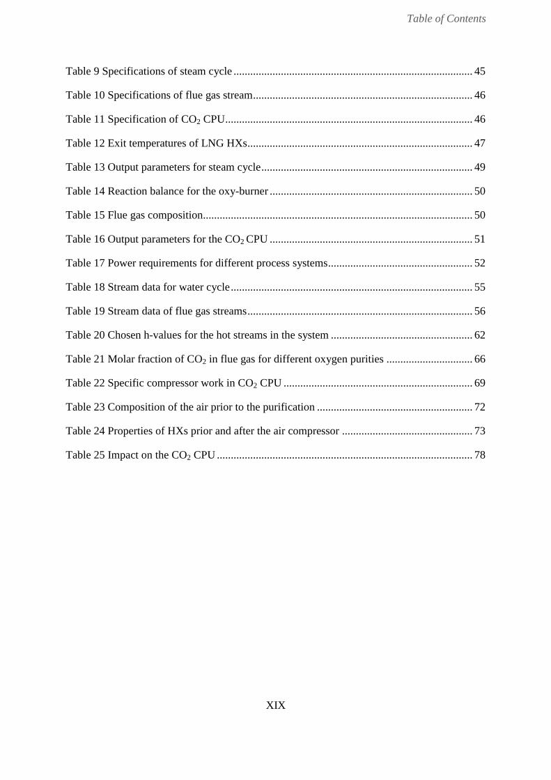
Table of Contents
XIX
Table 9 Specifications of steam cycle ...................................................................................... 45
Table 10 Specifications of flue gas stream ............................................................................... 46
Table 11 Specification of CO2 CPU ......................................................................................... 46
Table 12 Exit temperatures of LNG HXs ................................................................................. 47
Table 13 Output parameters for steam cycle ............................................................................ 49
Table 14 Reaction balance for the oxy-burner ......................................................................... 50
Table 15 Flue gas composition ................................................................................................. 50
Table 16 Output parameters for the CO2 CPU ......................................................................... 51
Table 17 Power requirements for different process systems .................................................... 52
Table 18 Stream data for water cycle ....................................................................................... 55
Table 19 Stream data of flue gas streams ................................................................................. 56
Table 20 Chosen h-values for the hot streams in the system ................................................... 62
Table 21 Molar fraction of CO2 in flue gas for different oxygen purities ............................... 66
Table 22 Specific compressor work in CO2 CPU .................................................................... 69
Table 23 Composition of the air prior to the purification ........................................................ 72
Table 24 Properties of HXs prior and after the air compressor ............................................... 73
Table 25 Impact on the CO2 CPU ............................................................................................ 78

XX

Introduction
1
1 Introduction
Global warming is one of the main challenges the world will face in the years to come.
Carbon dioxide (CO2) makes the largest anthropogenic contribution to global warming, where
fossil fuels like oil, gas and coal accounts for approximately 75 % of the anthropogenic CO2
emissions. The emissions of greenhouse gases can be reduced by use of alternative energy
sources, like renewable energy. However, renewable energy is not yet reliably to produce
sufficient power to meet the increasing energy demand. In addition, no renewable energy
sources are economical feasible to produce large quantities of energy. Thus combustion of
fossil fuels is likely to meet the immediate demand. To reduce emissions from fossil fuel
power plants, improving the overall efficiency can, to a certain point contribute to reduce CO2
emissions. But to sufficiently decrease the CO2 emissions it will be essential to develop
technology to capture and store the CO2 generated [1-3].
One of the fossil fuel sources that are relevant for CO2 capture is Natural Gas (NG). NG is a
growing energy source worldwide; according to Energy Information Administration (EIA) the
world’s natural gas consumption will increase with 44 % from 2007 to 2035 [4]. Compared to
Oil and Coal, NG is a more environmental friendly fuel. It emits less greenhouse gases, and
has higher relative fuel efficiency for a given amount of energy. The CO2 produced from oil
and coal is approximately 1.4 – 1.75 times higher than for NG. Thus, the increased
consumption of NG could lead to decreased CO2 emission if produced, and processed in a
more environmental friendly manner.
NG can be transported as compressed gas through pipelines or as Liquefied Natural Gas
(LNG), where the latter transportation technology is more convenient when the gas is to be
transferred over large distances. This is due to costs, safety and technical issues. When NG is
liquefied its volume is reduced, hence the specific energy content increases, making the
transportation economically feasible. NG is liquefied at approximately -160 ºC, and is
classified as a cryogenic liquid1. The LNG is transported to regasification terminals where it is
stored and vaporized before distributed to end users. As the production rate of LNG is likely
to increase in the years to come, several new regasification terminals are required. The heat
source for regasification of LNG is today either a burner system where a part of the NG
produced is utilized to produce heat to vaporize the LNG, or sea water. Both systems induce
local and global emissions to the atmosphere or the sea. To make NG production more
environmental friendly, Aker Solutions (AKSO) has developed a regasification technology
which offers minimal emissions. The objective is to limit external utility consumption by heat
integrating the LNG regasification unit with a power and steam plant. The CO2 from the
power facility will be captured by using oxy-fuel combustion technology. Thus the system
will manage to vaporize LNG without significant environmental impact [4, 5].
1 Cryogenic liquid: Below -150⁰C
Introduction
2
1.1 Background
The motivation for the zero emission regasification plant is the increased demand for natural
gas worldwide, and the regulations that require minimum emissions and effluent discharge to
the environment from such plants. Today the most common technology for vaporizing LNG is
Open Rack Vaporizers (ORVs), which uses ambient sea water as the heat source. The heat
exchanger consists of vertical aluminum panels, where sea water is fed at the top, flowing
downwards on the outside of the panels, while the LNG flows on the tube side. The
disadvantages of the system is that a considerable amount of water is required, resulting in
discharge of vast amounts of cold water to the sea. This induces a local temperature drop,
which harms marine life. The system is climate sensitive, and is therefore not an adequate
solution if the ambient sea water temperature tends to drop below 8 degrees during winter. In
addition the water is treated with chlorinate resulting in emissions to the sea [6].
In addition to the ORVs, Submerged Combustion Vaporizers (SCVs) are broadly used. In a
SCV the LNG is routed through tubes, submerged in a water bath. The water is heated by flue
gas from a burner combusting part of the send-out gas. The combustion products are
discharged to the atmosphere, causing both local and global emissions. The CO2 emissions
from a SCV system is approximately 310 000 tons/year for a NG production rate of 42.5
Sm3/day. This is equivalent to 850 tons CO2/day [7].
If new regasification units are to apply either the ORV or SCV technology this will result in
significant emissions. Research in new low-emission regasification technology is therefore
important to limit emissions from such plants.
1.2 Thesis structure and limitations
The main objective of this thesis is to look at opportunities of reducing the overall power
consumption of the regasification plant. As of today, the technology is not able to compete
economically with conventional regasification technologies. This is mainly due to the
cryogenic Air Separation Unit (ASU) and the CO2 capture, which contributes to large
efficiency penalties and high costs.
This thesis evaluates the heat integration solution proposed by AKSO to minimize the total
heat transfer area in the plant. Simulation models of the regasification terminal are made in
Aspen Hysys, and all data used to evaluate the system are extracted from these models. The
simulation model is made by the author and is based on utility flow diagrams of the plant. As
the author had no knowledge of Aspen Hysys, the simulation models could possibly be
simplified more than those used in this thesis.
The heat integration in the system is evaluated in terms of sequence of the stream matches, the
temperature profile for the intermediate heat carriers used and the use of steam. In addition to
evaluate the heat integration in the system, opportunities of integrating a cryogenic ASU are
discussed. As the cryogenic ASU includes complicated unit operators, a complete simulation
model of the ASU is not constructed. Since the main air compressor accounts for most of the

Introduction
3
power consumption in the ASU, only the compressor is simulated to quantify opportunities of
reducing the power consumption by using the ASU as a heat sink for the regasification unit.
Three different oxygen-purities are tested for the oxy-fuel burner to examine the impact on
the ASU and the CO2 Compression and Purification Unit (CPU). This part of the thesis is
limited by the reactor in the simulation model, which for simplicity, is simulated with
complete combustion.
The first chapter of this thesis describes the regasification concept planned by AKSO to give
the reader an understanding of the basis of the concept before the different technologies are
further described. In accordance with AKSO, all information regarding economics and all
utility flow diagrams are left out, including specifications found in these diagrams.
Chapter 3-7 presents theory regarding oxy-fuel combustion, ASU technology, heat integration
and membrane technology. This theory forms the basis for the simulation cases. For the ASU
only a brief introduction to distillation is given, as this is a broad subject and only an
understanding of the fundamentals is required for the discussion of the simulation model. In
Section 3.3 the fundamental of an oxy-fuel NGCC is described. The regasification plant
planned by AKSO is based on a steam cycle with a simple oxy-fuel burner. However, a basic
understanding of an oxy-fuel NGCC is required as most literature regarding NG fired oxy-
combustion, is based on NGCCs. In Chapter 7 an introduction to intermediate heat transfer
fluids is given. Though this heat transfer method is broadly used, the available theory is
limited. In Chapter 6 the fundamentals of membranes used for air separation is presented.
This subject is broad, and only membranes capable of producing high purity oxygen will be
discussed.
The description of the simulation models, and results from these models are discussed in five
different chapters. All the different chapters include methodology and results. It is chosen to
discuss the results throughout these chapters, instead of gathering all results in the end. This is
due to the fact that the results gained for the different simulation models are connected to each
other. The structure of these chapters is as follows:
Chapter 8: Describe which specifications and assumptions are applied in Aspen Hysys, when
creating the main simulation model. The last part of Chapter 8 discusses the results gained in
the main simulation model. It is chosen to have this discussion prior to the evaluation of the
system, as all data used in the evaluation is extracted from this chapter.
Chapter 9: Describes the methodology used to evaluate the heat integration in the system.
The results are given in the last part of the chapter. All data used to evaluate the system are
extracted from Chapter 8.
Chapter 10: Discuss the impact of changing the oxygen purity in the plant. Three different
oxygen purities are tested; 90, 95 and 97mol%.
Chapter 11: Based on results from Chapter 8-10, the possibility of integrating an ASU is
discussed.

Introduction
4
Chapter 12: Based on the previous chapter a proposed process solution is presented in this
chapter. In addition the possibility of using membranes for air separation is discussed. This is
limited to information extracted from literature, as it is not possible to simulate a membrane in
Aspen Hysys.
Introduction to Aker Solutions regasification concept
5
2 Introduction to Aker Solutions regasification concept
AKSO has developed a concept called; “Zero emission power production for LNG
regasification”. The objective of this concept is to develop a system that vaporizes and heats
LNG without CO2 emissions. In addition, the system is planned to be self contained with
power to make the system employable to off-shore sites. The system contains an LNG
regasification train, an oxy-fuel boiler system with power and steam generation and a CO2
purification and compression unit.
The following sections will explain the fundamentals of AKSO’s regasification system.
Details regarding the system configuration are collected from Aker Solutions Base Case
report [8].
2.1 Regasification unit
The regasification unit is the main unit of the facility; all other units provide power and heat
to the regasification train. According to the calculation from Aker Solutions’ study report, 736
kJ/kg LNG is required to vaporize and heat the LNG from -161 ⁰C to the required sales gas
temperature [8].
The cold LNG feed is pumped to 80 bar before entering the vaporization and heating section,
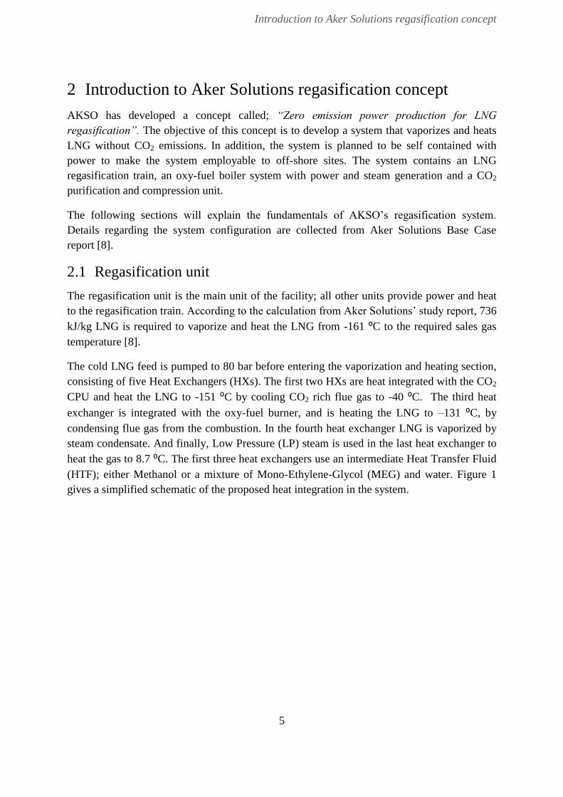
consisting of five Heat Exchangers (HXs). The first two HXs are heat integrated with the CO2
CPU and heat the LNG to -151 ⁰C by cooling CO2 rich flue gas to -40 ⁰C. The third heat
exchanger is integrated with the oxy-fuel burner, and is heating the LNG to –131 ⁰C, by
condensing flue gas from the combustion. In the fourth heat exchanger LNG is vaporized by
steam condensate. And finally, Low Pressure (LP) steam is used in the last heat exchanger to
heat the gas to 8.7 ⁰C. The first three heat exchangers use an intermediate Heat Transfer Fluid
(HTF); either Methanol or a mixture of Mono-Ethylene-Glycol (MEG) and water. Figure 1
gives a simplified schematic of the proposed heat integration in the system.

Introduction to Aker Solutions regasification concept
6
Figure 1 Heat integration between power cycle and LNG regasification unit
2.2 Oxy – fuel steam and power system
The oxy-fuel steam and power system provides heat and power to the facility, and consists of
an oxy-fuel burner, a steam boiler, a Low Pressure (LP) and a Medium Pressure (MP) steam
turbine. For oxy-fuel boilers, almost all literature refers to Pulverized Coal (PC) fired oxy-fuel
systems. AKSO has developed a similar NG fired oxy-fuel system. The fundamentals of oxy-
fuel combustion are discussed in Chapter 3.
Approximately 1.5 % of the send-out gas is sent to the oxy-fuel burner where it burns in an
oxygen rich environment. To control the flame temperature, a considerable amount of the
CO2-rich flue gas is recycled to the burner. The recycle rate is controlled to limit the flame
temperature to1450⁰C. The flue gas from the oxy-burner is cooled by preheating Boiler Feed
Water (BFW), generate steam and superheat the MP steam before it is further processed in the
CO2 CPU. Figure 2 shows a simplified schematic of the oxy-fuel burner and steam boiler.

Introduction to Aker Solutions regasification concept
7
Figure 2 Simple schematic of the oxy-fuel steam and power system
The superheated MP steam from the boiler is routed through a two stage turbine where it is
expanded to produce the required electrical energy; approximately 34 MW. The power
demand in the facility equals the production rate; hence no power is exported. A portion of
steam leaving the MP turbine is drawn-off and used to heat NG, oxygen and fuel prior to the
burner. The oxy-fuel plant is planned to operate at 100% of design capacity. The turndown
requirement is assumed to be 40%.
2.3 Air separation unit
Oxygen is separated from ambient air by cryogenic distillation in an ASU. The ASU provides
95mol% pure oxygen, and produces 1181 tons/day at full capacity. In AKSO’s base case, the
ASU is not heat integrated with the power plant, thus it accounts for a significant part of the
overall power consumption. AKSO’s calculations show that 33% of the power produced is
required to run the ASU.
The ASU in AKSO’s concept is based on Linde’s dual reboiler configuration (further
explained in Section 4.2). The air is compressed to approximately 4.4 bar in three stages with
intercooling. Cooling Water (CW) is used as the external cold utility. The air is then filtered
and dried by a molecular sieve, before cooled to -192⁰C in the main heat exchanger. Air is
then separated to N2 and O2 by cryogenic distillation. To produce 1181 tons of oxygen per
day, 7000 kmol ambient air/h, is required. When the oxy-fuel plant is turned down the excess
oxygen produced is stored in buffer tanks.
2.4 CO2 compression and purification unit
The flue gas from the oxy-fuel burner is routed to the CO2 CPU where it is cooled to 20⁰C by
heating LNG. The flue gas is then sent to a scrubber where the bulk of water is removed.
Approximately 87.9 % of the CO2 rich flue gas is recycled to the oxy-fuel burner to maintain
the flame temperature, while the remaining flue gas is compressed and further cooled and
dehydrated. The cooled CO2 gas is sent to a cryogenic distillation column where a CO2 liquid
stream is recovered at the bottom, while a nitrogen and oxygen rich gas leaves the vessel as

Introduction to Aker Solutions regasification concept
8
distillate. The CO2 is further compressed and heated before exported or stored in underground
storage.
2.5 Overall plant performance
At full capacity, the flow of LNG feed is estimated to 25 MillionSm3/day. 1.5% of the sales-
gas is burnt in the oxy-fuel burner. The production rate of CO2 is estimated to be about 796
tons/day. With a CO2 recovery rate of 92%, the CO2 emissions will be approximately 65
tons/day. This equals 7.6% of the CO2 emissions from a SCV. It is important to notice that the
CO2 emission from the system is dependent on the application of the distillate from the
N2/CO2 separation. If the gas is vented, the emission will be as stated above.
The system requires a CW recirculation system for cooling air prior to the cold box in the
ASU; this is the only cold utility requirement in the plant. When running at full capacity, the
heat required to vaporize the LNG is calculated to 157.7MW. Most of the heat (123 MW) is
provided by either steam or steam condensate produced in the plant.
The overall power consumption by the different units in the plant is given in Table 1. The
numbers are extracted from simulation models created in Aspen Plus.
Table 1 Power requirement of the different process systems
Process system Duty
[MW]
ASU 11.3
LNG pumps 4.3
Flue gas fan 4.2
Flue gas recycle fan 1.5
CO2 compressors and pumps 3.1
BFW pump 0.5
CO2 heater (air fan) 2.3
20 % margin for others 6.8
SUM 34

CO2 Capture and storage
9
3 CO2 Capture and storage
One way of reducing CO2 emissions is to develop CO2 capture plants for fossil-fired power
generation. Carbon Capture and Storage (CCS) is intended to be installed at large point
sources of emission, including NG fired power plants. There exists three main CO2 capture
technologies currently being investigated; post-combustion CO2 capture, pre-combustion CO2
capture and oxy- fuel combustion CO2 capture. The latter technology will be referred to as
oxy-combustion in the following. In post combustion, CO2 is separated from the flue gas by
absorption or another separation technology. In pre-combustion, the fuel is converted to
syngas (H2 and CO), which is shifted to H2 and CO2 by the presence of steam. CO2 can then
be captured prior to the combustion. Oxy-combustion is combustion of fuel in an oxygen rich
environment, which results in a CO2-rich flue gas, making it easier to separate the CO2. None
of these CCS technologies are economically feasible today. Some of the main challenges
researchers encounter when trying to find solutions for CO2 capture, are economics, the time
CO2 can be stored, the means of transporting the CO2 and technological issues [9, 10].
This thesis will focus on oxy-fuel combustion, and in the following a description of the
technology will be given and two different oxy-combustion configurations will be presented.
Technological issues regarding oxy-fuel combustion will be discussed.
3.1 CO2 capture by oxy-fuel combustion
In conventional air combustion the nitrogen content is approximately 79 mol% and dilutes the
CO2 concentration in the flue gas, making CO2 capture complicated and expensive. In oxy-
combustion the combustion takes place in an oxygen rich environment, i.e. the molar fraction
of oxygen are typically between 90 – 97mol%. Because of the high oxygen purity, the flue
gas becomes enriched in CO2, making CO2 capture less complicated. The water is condensed
to get the CO2 for deposing, and CO2 is separated from the flue gas.
Though the flue gas mainly consists of CO2 and water, other impurities will be present. In a
complete stoichiometric combustion, the fuel reacts with the exact amount of oxygen required
to oxidize all the carbon in the fuel to CO2, and the hydrogen to H2O. For a real combustion
however, the flue gas will consist of other substances like CO, NOx and O2. CO is produced
both in lean and rich combustion, where the first is combustion where the Air Fuel -ratio (AF)
is below that of stoichiometric combustion and the latter is combustion where the AF is
higher than that of stoichiometric combustion. In lean combustion CO is formed as a result of
the dissociation of CO2, and because of the lack of oxygen. The NOx and N2O amount formed
in combustion stem from the nitrogen in the air used for the combustion. The NOx formation
is dependent on temperature, time and oxygen availability. In oxy-combustion the NOx
formation is lower compared to conventional combustion due to the low N2 concentration in
the furnace. For lignite fired oxy-combustion the NOx emissions has been reported to be 50 %
lower than for conventional air fired combustion [11, 12].
CO2 Capture and storage
10
Oxy-combustion differs from conventional combustion in several ways; in conventional air
supported combustion, nitrogen has a minor chemical effect, but a large thermodynamic
impact as it absorbs heat during the combustion. Thus, the flame temperature in oxy-
combustion will exceed that of conventional air combustion. The flame temperature reaches
3500 ⁰C, which can cause complications in the burner. To reduce the combustion temperature
either part of the CO2 rich flue gas has to be recycled or water injected. In addition to
increased flame temperature, the flue gas volume is reduced and the density of the flue gas is
increased due to the high molecular weight of CO2 which exceeds that of N2 [1, 13].
The main reasons why CCS is not yet commercially available is the cost and risks of CCS
which overweigh the commercial benefits. In addition, the regulatory framework for CO2
storage is not sufficiently defined, and the power consumption for an oxy-fuel system is
significantly higher than for a conventional plant, mainly due to extra units operators [5, 14].
3.2 CO2 Compression and purification
Implementing CCS to oxy-fuel configurations results in significant auxiliary power load. The
compressor work in the ASU and the CO2 CPU are the main causes of the increased power
consumption. Therefore reducing the CO2 compression work is an important parameter in
commercializing oxy-fuel combustion. In the following the fundamentals of compression will
be presented and the design parameters of the CO2 CPU discussed.
3.2.1 Fundamentals of compression
For a reversible compressor neglecting changes in potential and kinetic energy, compression
work can be expressed as [15]:
2
int 1rev
Wvdp
m
(3.1)
Where m [kg/s] is the mass flow rate, W [kW] is the compressor work and v [m3/kg] is the
specific volume. If integrating Eq.(3.1) for a polytrophic compression (i.e. a real compression)
the specific work can be expressed as [16]:
1
21 1
1
11
n
npnW Z RT
n p
(3.2)
Where Z is the compressibility factor, n is the polytrophic index, T1 is the compressor inlet
temperature, P1 [kPa] is the inlet pressure and P2 is the outlet pressure. R [kJ/kgK] is the gas
constant, expressed as the ratio between the universal gas constant Ro (8.314 kJ/kmolK] and
the molecular weight M [kg/kmol]

CO2 Capture and storage
11
As can be seen from Eq.(3.2), the inlet temperature T1 plays an important role for the
magnitude of the compression work. The temperature ratio in a compressor can be expressed
in terms of the pressure:
1
2 2
1 1
n
nT p
T p
(3.3)
Where n can be calculated from:
1
p
p
nk
k
(3.4)
Where np is the polytrophic efficiency for the compressor, and k is the isentropic index, which
is given by the ratio of heat capacity at constant pressure (Cp) and heat capacity at constant
volume (Cv).
From Eqs.(3.2) and (3.3), it can be seen that a low inlet temperature will decrease the
compressor work, if the pressure ratio if fixed. From Eqs.(3.2) and (3.4), it can be seen that
for a constant polytrophic efficiency a high k-value results in lower power consumption for
the same pressure ratio. The compressor work is also affected by the molecular weight of the
gas, as W is a function of the gas constant. A high molecular weight will result in a lower R-
value, hence the specific work will decrease.
3.2.2 CO2 CPU design
The objective of the CO2 CPU is to compress the flue gas and condense most of the water,
before the CO2 is purified and pumped to the required product pressure. The combination of
compression, condensation and pumping reduces the overall power consumption. In most
CO2 CPU configurations, the flue gas is compressed in several stages with intercooling. By
dividing the compression in a number of stages the net work required by each compressor are
reduced. The gas is cooled and water removed between each compression step. Water needs
to be removed in several stages because the solubility of water in CO2 decreases with
pressure. The effect of multistage compression with intercooling for an isentropic compressor
can be seen in the pressure-enthalpy diagram(Figure 3) [8, 17].

CO2 Capture and storage
12
Figure 3 Multistage compression with intercooling [18]
For a one stage compressor with pressure ratio p2/p1 the total enthalpy increase is h2-h1. If the
gas is compressed in three stages, and cooled near its saturation line between each stage, the
compression work will decrease as can be seen from the graph above. The total enthalpy
increase can then be expressed as (h7-h6) + (h5-h4) + (h3-h1).
There exist different CO2 CPU configurations. The choice of configuration is dependent on
the fuel used (NG or PC), desired CO2 recovery rate, product specifications and the trade-off
between Capital expenses (CAPEX) and operating expenses (OPEX). There exist three main
CO2 CPU schemes. If a 100 % CO2 recovery rate is required the CO2 CPU can be designed
with no purification, meaning that the flue gas is only compressed and cooled with no
separation of N2/CO2. Another solution is partial condensation in a cold box. In this scheme
the flue gas is compressed and dehydrated before cooled to a very low temperature to
condensate most of the CO2. This scheme has a 90% CO2 recovery rate. An extension of this
configuration is a scheme with cryogenic distillation, where the flue gas is purified by
distillation after the cold box. This results in a purer product stream; it can exceed 99 %
depending on the scheme. If using cryogenic distillation, the separation should take place
between the triple point (5.1795 bar and -56.6 ⁰C) and the critical point (73.773 and 31.03 ⁰C)
of CO2, meaning that the partial pressure of CO2 should exceed 5.1795 to experience a phase
change [10, 19]. Figure 4 shows the specific power of the CO2 CPU for the different
configurations as a function of the CO2 content in the flue gas.
CO2 Capture and storage
13
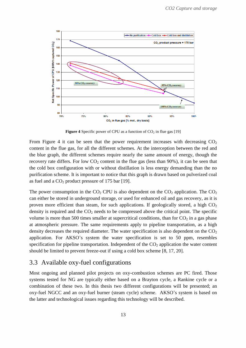
Figure 4 Specific power of CPU as a function of CO2 in flue gas [19]
From Figure 4 it can be seen that the power requirement increases with decreasing CO2
content in the flue gas, for all the different schemes. At the interception between the red and
the blue graph, the different schemes require nearly the same amount of energy, though the
recovery rate differs. For low CO2 content in the flue gas (less than 90%), it can be seen that
the cold box configuration with or without distillation is less energy demanding than the no
purification scheme. It is important to notice that this graph is drawn based on pulverized coal
as fuel and a CO2 product pressure of 175 bar [19].
The power consumption in the CO2 CPU is also dependent on the CO2 application. The CO2
can either be stored in underground storage, or used for enhanced oil and gas recovery, as it is
proven more efficient than steam, for such applications. If geologically stored, a high CO2
density is required and the CO2 needs to be compressed above the critical point. The specific
volume is more than 500 times smaller at supercritical conditions, than for CO2 in a gas phase
at atmospheric pressure. The same requirements apply to pipeline transportation, as a high
density decreases the required diameter. The water specification is also dependent on the CO2
application. For AKSO’s system the water specification is set to 50 ppm, resembles
specification for pipeline transportation. Independent of the CO2 application the water content
should be limited to prevent freeze-out if using a cold box scheme [8, 17, 20].
3.3 Available oxy-fuel configurations
Most ongoing and planned pilot projects on oxy-combustion schemes are PC fired. Those
systems tested for NG are typically either based on a Brayton cycle, a Rankine cycle or a
combination of these two. In this thesis two different configurations will be presented; an
oxy-fuel NGCC and an oxy-fuel burner (steam cycle) scheme. AKSO’s system is based on
the latter and technological issues regarding this technology will be described.

CO2 Capture and storage
14
3.3.1 Oxy-fuel NGCC
A conventional NGCC consist of a gas turbine, with air as the working fluid, combined with a
steam cycle. Figure 5 shows a semi closed oxy-fuel combined cycle. The working fluid in the
cycle is diluted CO2, which is used to limit the flame temperature. The flue gas is sent through
a heat recovery steam generator (HRSG), generating steam that is utilized in a two stage
turbine. Water is removed from the flue gas, and CO2 is captured. Because diluted CO2 is used
as the working fluid, the gas turbine needs to be redesigned. When using diluted CO2 an
increased speed of sound is experienced (80% higher than for air), resulting in a lower mach
number. The density is approximately 50% higher for CO2, and the specific heat ratio is lower
which results in a lower temperature change in an adiabatic compression or expansion. The
optimal pressure ratio is higher for oxy-fuel NGCCs than for a conventional cycle. Typically
30-35, compared to 15-18 for a conventional gas turbine. A higher pressure ratio increases the
required compressor work, hence the efficiency will decrease. The efficiency for a typical
oxy-fuel combined cycle is approximately 45 – 47%, which is nearly 10 % less than for a
conventional combined cycle [10, 13].
Figure 5 oxy-fuel combined cycle with steam generation [13]
3.3.2 Oxy-fuel burner
Retrofitting a conventional gas turbine to oxy-fuel combustion is complicated because the
working fluid differs from that of a conventional gas turbine. Another configuration which
can be used is an NG fired oxy-fuel burner with steam generation. NG is combusted in an
oxygen rich environment producing a CO2 rich flue gas. In most oxy-fuel boiler
configurations, a part of the flue gas is recycled to the burner to limit the flame temperature.
The remaining part of the flue gas is sent to the CO2 purification unit were water is drained
out, and the gas is compressed and purified as explained in Section 3.2.2.
CO2 Capture and storage
15
Studies on PC fired oxy-burners indicate that conventional burners can be retrofitted to oxy-
fuel, but there are several challenges to overcome before oxy-fuel boilers are feasible [21].
The next section will explain the most critical technological challenges.
Technical challenges for oxy-fuel burners
Increased heat transfer for oxy-fuel burners compared to air-combustion is expected. The
main reason is the increased concentration of tri-atomic (molecules formed by three atoms)
gases in the furnace. These molecules absorb and emit radiation, resulting in an improved
radiative heat transfer. In addition, CO2 and water has higher specific heat capacity than
nitrogen, resulting in increased heat transfer in the convective heat transfer zone [22].
The change in flame characteristics is one challenge researchers need to overcome to be able
to manufacture oxy-fuel boilers or retrofit existing boilers. But according to Bensakhria and
Leturia [22], the flame characteristics for oxy-combustion can be adjusted to give the same
conditions as for conventional combustion. Another challenge for oxy-fuel boilers is the
recycle ratio. As opposed to conventional burners, which operate at a fixed excess air ratio
and air composition, an oxy-fuel burner needs to be custom-made. The configuration of the
burner is dependent on the recycle rate which differs with oxygen purity and fuel
composition.
According to a study carried out by SINTEF Energy AS for AKSO, there are three suppliers
with experience in natural gas oxy-fuel burners for CCS; Air Liquid, Clean Energy System
and Jupiter Oxygen [5]. Jupiter Oxygen has tested an NG fired oxy-boiler, without recycling
flue gas. As already mentioned, oxygen rich combustion leads to extremely high flame
temperatures, mainly because of the increased heat transfer in the radiative zone. According to
Jupiter Oxygen simulations, the radiant zone increases by 31 % for oxy-fuel combustion
compared to conventional air combustion. As the heat flux from radiation is proportional to
T4, the increased flame temperature result in a significant heat flux. Jupiter Oxygen has
developed a boiler which tolerates these high temperatures by limiting the heat flux, thus no
reflux is needed making it more economically feasible to retrofit existing steam boilers [23].

Air separation technology
16
Air separation technology
17
4 Air separation technology
There exists different air separation technologies; Adsorption, membrane and cryogenic
distillation. In the following chapters, the two latter technologies will be described.
Adsorption is not further discussed, as this technology is not economically feasible for oxygen
production above 200 tons/day [13].
4.1 Distillation
The most complex unit operation in an ASU is the cold box where all the cryogenic
equipments are located, including the main heat exchanger and the cryogenic distillation
column. To understand the structure of an ASU a brief introduction to distillation is presented
in this section.
In a single-stage separation of a homogenous mixture, the mixture is partly vaporized and the
components are separated based on their difference in boiling point. A single separation stage
can only achieve a limited separation, thus to increase the separation rate the components can
be separated by distillation. A distillation column can be thought of as several single stage
separators where the feed enters the column as liquid, vapor or a mixture. In the column, a
part of the feed vaporizes and flows upwards, while the liquid flows downwards. The less
volatile components will be transferred to the liquid phase, while the more volatile
components are transferred to the vapor phase. The liquid leaving the bottom of the column is
partly of totally vaporized in a reboiler and routed back to the column. The vapor leaving the
top of the column is partly or fully condensed before routed back to the column as reflux, to
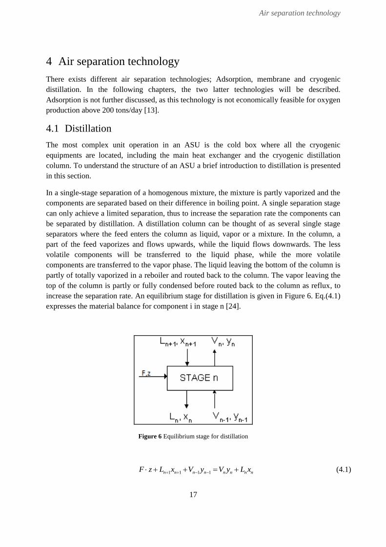
increase the separation rate. An equilibrium stage for distillation is given in Figure 6. Eq.(4.1)
expresses the material balance for component i in stage n [24].
Figure 6 Equilibrium stage for distillation
1 1 1 1n n n n n n n nF z L x V y V y L x (4.1)

Air separation technology
18
F is the feed, L is the flowrate of liquid and V is the flowrate of vapor. The rate of distillation
is dependent on the K value and the relative volatility of the mixture. The K for component i
is given in the equation below [25]:
ii
i
yK
x (4.2)
Where yi is the mole fraction of component i in the vapor phase, and xi is the mole fraction of
component i in the liquid phase. The K value is a measure of the tendency of component I to
vaporize and is dependent on temperature, composition and pressure. For a binary mixture,
the separation of components in a distillation is dependent on the ratio of the K value for
component i and j, respectively. This ratio is called the relative volatility and is expressed by
Eq.(4.3). If the relative volatility is high one component has a much greater volatility than the
other, making the separation easier.
,i
i j
j
K
K (4.3)
There are several operating conditions affecting the distillation column; operating pressure,
reflux ratio, condition of the feed, type of condenser and number of stages. There exists a
trade-off between these operation conditions E.g. if the operating pressure is raised the
separation becomes more difficult, but the condenser/reboiler duties are decreased. Therefore
the accurate design of the column is of great importance [24].
4.2 Cryogenic air separation unit
An oxy-fuel steam and power plant requires an oxygen production greater than 1000 tons/day.
Today, cryogenic distillation is the only available technology to produce large quantities of
high purity oxygen. There exists several different ASU configurations; in the following the
basics of cryogenic distillation with double column will be explained.
An ASU mainly consist of air compressors, a purification unit and a cold box, containing the
main HX and the distillation column, both operating at cryogenic temperatures. Ambient air is
fed to the air compression and purification unit where it is compressed to about 5 bar before it
is purified. Ambient air typically contains 21% oxygen, 0.04 % CO2, 1% H2O, 0.9% Argon
and 77.1 % N2.The water and CO2 content is limited to prevent freeze out in the cold box, as
both components have a higher boiling points than both oxygen and nitrogen. The air is then
routed to the cold box where it is cooled to or below its dew point before entering the
rectification section, which consists of two integrated distillation columns. The columns are
integrated by having a condenser-reboiler that furnish reflux for the bottom column and vapor
for the upper one. Air enters the bottom of the HP column partially liquefied. In the HP
column vapor, enriched in nitrogen, is rising to the HP condenser. The liquid nitrogen from
the condenser is split into two different reflux streams for both the HP column and the LP
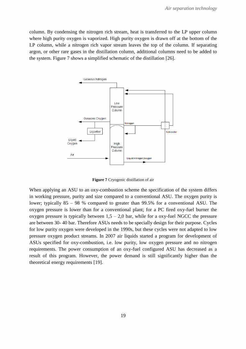
Air separation technology
19
column. By condensing the nitrogen rich stream, heat is transferred to the LP upper column
where high purity oxygen is vaporized. High purity oxygen is drawn off at the bottom of the
LP column, while a nitrogen rich vapor stream leaves the top of the column. If separating
argon, or other rare gases in the distillation column, additional columns need to be added to
the system. Figure 7 shows a simplified schematic of the distillation [26].
Figure 7 Cryogenic distillation of air
When applying an ASU to an oxy-combustion scheme the specification of the system differs
in working pressure, purity and size compared to a conventional ASU. The oxygen purity is
lower; typically 85 – 98 % compared to greater than 99.5% for a conventional ASU. The
oxygen pressure is lower than for a conventional plant; for a PC fired oxy-fuel burner the
oxygen pressure is typically between 1,5 – 2,0 bar, while for a oxy-fuel NGCC the pressure
are between 30- 40 bar. Therefore ASUs needs to be specially design for their purpose. Cycles
for low purity oxygen were developed in the 1990s, but these cycles were not adapted to low
pressure oxygen product streams. In 2007 air liquids started a program for development of
ASUs specified for oxy-combustion, i.e. low purity, low oxygen pressure and no nitrogen
requirements. The power consumption of an oxy-fuel configured ASU has decreased as a
result of this program. However, the power demand is still significantly higher than the
theoretical energy requirements [19].

Possibilities of power reduction
20
Possibilities of power reduction
21
5 Possibilities of power reduction
If oxy-fuel combustion shall be commercialized, reduction in CAPEXs, OPEXs and power
consumptions is required. One possibility is integrating the ASU with the power plant. This is
an instinct subject, due to lack of research on the matter. Another possibility is to change the
oxygen purity. Both the power consumption in the ASU and the CO2 CPU is a function of the
oxygen purity, therefore it is essential to investigate the subject to find the ideal purity for the
plant. In the following these subjects will be discussed.
5.1 Integration between an ASU and an oxy-fuel power cycle
Integrating an ASU with an oxy-fuel combustion system is proven difficult, due to the rigid
integration within the ASU cold box. Air is cooled to cryogenic temperatures by returning
streams from the distillation train, i.e. the cold box is fully heat integrated [8].
For oxy-fuel NGCCs there exists some integration concepts. Compressed air can be drawn
from the gas turbine’s compressor, and fully or partially supply the feed requirements of the
ASU. As the distillation pressure will be set by the extraction air pressure, a supplemental air
compressor is necessary if the mass flow from the turbine is less than the required mass flow
in the ASU. Another solution for an NGCC is to compress the byproduct nitrogen, and heat it
against the extracted air from the gas turbine. This will lead to heat recovery, as the extracted
air needs to be cooled before entering the ASU. By injecting nitrogen into the gas turbine the
NOx emission are reduced, as nitrogen reduces the flame temperature and thus the production
of NOx [27].
For oxy-fuel boilers, heat integration with an ASU includes heat transfer from the air
compressors to the steam and power production unit. The surplus heat can be used to preheat
BFW, preheat oxygen prior to the combustion, or it can be used to heat other cold streams in
the plant. Because of the rigid integration in the cold box, thermal integration is limited to
recover heat of compression.
AKSO has evaluated the possibility of integrating the ASU with the regasification unit. It was
found complicated because turn-down of the ASU during off-peak demand, is difficult. This
flexibility problem is the most prominent issue regarding the subject. According to Dubettier
et al. [28], the air compressors can achieve a turn down of 75% and the cold box a turn down
of 50% for a one train ASU configuration. If a further turn-down is required the excess
oxygen can be stored in buffer tanks. Air Liquid (AL) has developed a new concept called AL
Innovative Variable Energy where excess oxygen is stored as liquid during off-peak [19].
As already mentioned, integration between an ASU and an oxy-plant is not broadly
investigated. However, AL has tested a lignite fired oxy-fuel boiler, integrated with a
cryogenic ASU. The electric efficiency of the plant was increased by 1%, when heat
integrating the air compressors with the oxy-combustion plant. Research was done on an ASU

Possibilities of power reduction
22
with both 95 and 99%-volume oxygen purity. The high purity scheme only decreased the
overall efficiency by 1 %. This is an important result as higher oxygen purity result in lower
cost of the CO2 CPU. This is further discussed in the following section [29].
5.2 Impact of changing the oxygen purity
The following sub-chapters will discuss the impact of changing the oxygen purity. As the
literature on NG fired oxy-fuel boilers are limited, these chapters are based on literature
regarding PC fired oxy-fuel boiler and oxy-fuel NGCCs.
5.2.1 Impact on the ASU
When increasing the oxygen purity the energy demand in the ASU increases. Figure 8
demonstrates the energy of separation in an ASU, as a function of the oxygen purity. Energy
of separation [kWh/t] is defined as the power required producing 1 ton of gaseous oxygen at 1
atm.
Figure 8 Power requirement of a cryogenic ASU [19]
The graph in Figure 8 is quite rectilinear below 95mol% purity. At 97mol% oxygen purity,
the energy of separation increases sufficiently. This is because the separation changes from
oxygen-nitrogen to oxygen-argon in the LP column. This leads to increased power demand, as
well as increased CAPEX and OPEX.
The main energy-consuming component in an ASU is the air compressors. The power
consumption in the air compressors is dependent on the air feed flow and the outlet pressure,
hence it is dependent on the oxygen purity. According to a study carried out by Amann et al.
[2] the HP column pressure needs to be increased with 30 %, if changing the purity from 85
mol% to 97 %. The study was carried out for a NGCC converted to oxy-fuel. The results from
the study are given in Table 2.

Possibilities of power reduction
23
Table 2 Influence on ASU by changing the oxygen purity [2]
O2 purity [mol%] 85 90 95 97
O2 stream flow [tons/h] 271.7 255.7 241.4 236.8
ASU power [MW] 60.1 61.2 62.8 63.6
Specific consumption [kWh/tO2] 221.3 239.2 260.2 268.7
ASU penalty [%] 5.4 5.8 6.2 6.3
The results in Table 2 are from simulations performed in Aspen Plus. The oxygen stream flow
is calculated with 5 mol% excess oxygen in the flue gas. The air feed to the ASU is specified
to 279 kg/s. The ASU penalty corresponds to the difference in electric efficiency for the oxy-
fuel system, and a conventional Integrated Gasification Combined Cycle (IGCC). The ASU
power calculated is the electric power required in the air compressors [2].
From Table 2 it can be seen that the required oxygen flow decreased with oxygen purity. This
is because less oxygen is required to maintain a near-complete combustion in the furnace. The
compressor power of the ASU increases with increased oxygen purity. However, the increase
is relatively small, because of the reduced flow rate. Though the change in compressor work
is minor, the OPEX of the ASU will increase for increasing oxygen purity, due to the alternate
separation operation. Though the power consumption decreases with decreasing oxygen
purity, the required ASU equipment size will increase for oxygen purities below 95 mol%,
due to the inferior pressure in the system. This results in increased capital costs [30].
5.2.2 Impact on the CO2 CPU
As can be seen from Figure 8, oxygen purities above 95% are not favorable for the ASU.
However, it has a positive impact on the CO2 recovery process. With high oxygen purity the
CO2 concentration in the flue gas increases and the required molar flow of oxygen is reduced,
resulting in a lower flow rate of flue gas in the CO2 CPU. As a result, the compression work
in the CO2 CPU is reduced. In addition, the energy of separation in the distillation column is
reduced, due to the increased CO2 content in the flue gas. This can be seen from Figure 9,
showing the specific work of a CO2 CPU as a function of the CO2 content in the flue gas, for
different capture schemes (explained in Chapter 3).

Possibilities of power reduction
24
Figure 9 Specific work of CPU as a function of CO2 in flue gas [19]
Amann et al. study also examines the impact on the CPU, when changing the oxygen purity.
Oxygen purities between 85-97mol% have been tested for a CO2 CPU is with cryogenic
distillation. The result from the study is given in Table 3, and it shows that both the
compressor work in the CO2 CPU and the recovery process power are dependent on the
oxygen purity. In addition the waste expansion power will depend on the flue gas flow, which
changes with oxygen purity [2].
Table 3 Performance of the cryogenic CO2 recovery process [2]
O2
purity
[mol%]
Recovery
rate [%]
Flue gas flow
[kg/s]
CO2
compression
[MW]
Recovery
process power
[MW]
85 75.0 58.0 4.0 19.1
97 75.0 48.3 3.4 15.2
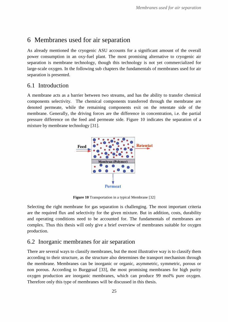
Membranes used for air separation
25
6 Membranes used for air separation
As already mentioned the cryogenic ASU accounts for a significant amount of the overall
power consumption in an oxy-fuel plant. The most promising alternative to cryogenic air
separation is membrane technology, though this technology is not yet commercialized for
large-scale oxygen. In the following sub chapters the fundamentals of membranes used for air
separation is presented.
6.1 Introduction
A membrane acts as a barrier between two streams, and has the ability to transfer chemical
components selectivity. The chemical components transferred through the membrane are
denoted permeate, while the remaining components exit on the retentate side of the
membrane. Generally, the driving forces are the difference in concentration, i.e. the partial
pressure difference on the feed and permeate side. Figure 10 indicates the separation of a
mixture by membrane technology [31].
Figure 10 Transportation in a typical Membrane [32]
Selecting the right membrane for gas separation is challenging. The most important criteria
are the required flux and selectivity for the given mixture. But in addition, costs, durability
and operating conditions need to be accounted for. The fundamentals of membranes are
complex. Thus this thesis will only give a brief overview of membranes suitable for oxygen
production.
6.2 Inorganic membranes for air separation
There are several ways to classify membranes, but the most illustrative way is to classify them
according to their structure, as the structure also determines the transport mechanism through
the membrane. Membranes can be inorganic or organic, asymmetric, symmetric, porous or
non porous. According to Burggraaf [33], the most promising membranes for high purity
oxygen production are inorganic membranes, which can produce 99 mol% pure oxygen.
Therefore only this type of membranes will be discussed in this thesis.

Membranes used for air separation
26
Inorganic membranes include symmetric/asymmetric single wall membranes, multilayer
asymmetric membranes and membranes with modified structure. These membranes can either
be dense or porous where the first denotes membranes made of solid layers of metal or mixed
conducting oxides, and the latter membranes made of a porous wall/top layer. The most
promising inorganic membranes for oxygen separation are ion transport membranes (ITMs).
These membranes are made of solid inorganic ceramic materials, and produces oxygen by
transferring oxygen ions (O2-
) trough the membrane. The driving forces are either the
difference in the partial pressure, or an electric voltage gradient. Membranes utilizing pressure
difference as the driving force, are referred to as mixed conduction membranes or mixed
ionic-electronic conducting membranes (MIECs), as they conduct both oxygen ions and
electrons [33]. The two different membrane concepts are given in Figure 11.
Figure 11 Different membrane concept: a) mixed conducting membrane,
b)electrical driven membrane [34]
ITMs have the potential of producing several tons of oxygen and are seen as one of the most
promising alternatives to cryogenic distillation, especially the MIECs since no electric circuit
is required to enhance electronic transport [34, 35].
6.2.1 Transportation mechanism of inorganic membranes
The transport mechanism for inorganic membranes are either Knudsen diffusion, selective
surface flow, molecular sieving or ionic transportation, where the latter is most common for
dense inorganic membranes used for gas separation [31].
If assuming constant ionic conductivity, the flux of oxygen through a MIEC is given by the
Wagner equation:
2
2
2
`
2 2 ``ln
4
OiO
O
pRTj
Ln F p
(6.1)
Where j is the oxygen flux through the membrane, R is the ideal gas constant, σ is the ionic
conductivity, n is the charge and F is the Faraday’s constant. P’ is the partial pressure of
oxygen in the air (feed side), and P’’ is the partial pressure at the permeate side. As can be

Membranes used for air separation
27
seen from this formula, the flux is proportional to ln(p1/p2) rather than the pressure difference
over the membrane [36].
Membranes are also characterized according to their permeability and selectivity. The
permeability denote the quantity of the solute gas diffusing through the solid pr second pr area
through a 1 m thick solid under a pressure of 1 atm. i.e. it denotes the amount of gas the
membrane is able to selectivity transfer per second. The permeability is given by the product
of solubility (S) and the diffusion (D) through the membrane (Eq.(6.2)). Where solubility
denotes the pressure normalized amount of gas sorbed in the membrane under equilibrium
conditions [10, 37].
M ijP D S (6.2)
The selectivity denotes the separation factor, and is expressed by the mole fraction or the
partial pressure of the gas components in the feed(x) and permeate (y) respectively. A high
selectivity provides a high purity. Eq.(6.3) denotes the selectivity (α) for a gas stream of two
components( i,j) [10, 31].
,
/
/
i j
i j
i j
y y
x x (6.3)
In MIECs an ionic current of oxygen is transferred through the membrane, while a
simultaneous flux of electrodes is transferred in the opposite direction. Oxygen is transported
from the high oxygen chemical potential side to the low potential side. Because oxygen is
transported in ionic form instead of molecular diffusion, the selectivity can theoretically reach
100 %. These membranes are thermally activated and the operation temperature is typically
between 700 ⁰C and 1000 ⁰C [34, 38].
6.2.2 Structure of MIECs
Finding the ideal membrane structure is challenging, and there exists several papers
researching the composition and structure of MIECs [38, 39]. This thesis will only introduce
the most promising materials in terms of oxygen flux and selectivity.
The most promising MIECs in terms of oxygen permeation, exhibit either a fluorite or
perovskite structure. This report will focus on the latter, as they tend to have a higher flux.
Perovskites have a cubic lattice, but it can be distorted into an orthorhombic structure which
makes it stable at high temperatures. The ideal perovskite (Figure 12), has the chemical
formula ABO3, where A, and B are metal ion with positive charge (cations) and O denotes
oxygen molecules with negative charge (anions). A is typically barium, lanthanum or
strontium, while B is typically cerium, cobalt or iron [38].

Membranes used for air separation
28
Figure 12 Ideal Perovskite [40]
If the perovskite had been ideal as in Figure 12, it would not be able to transport an ionic
current. Some defects are required to enhance ionic transportation. Vacancies are a form of
defects, and a high amount of vacancies gives a high oxygen permeation flux. There are many
different strategies employed to enlarge the oxygen permeation properties. The most common
strategy is doping the perovskite. Generally the ABO3 is improved by doping the B-site with a
more stable cation [34].
6.2.3 Performance of MIECs
Figure 13 Factors influencing the MIEC[39]
Figure 13 shows different factors that influence the membrane selection. Firstly the membrane
must possess high oxygen flux. The flux is influenced among others, by temperature,
pressure, membrane thickness and structure. As can be seen from Figure 14 the temperature
plays an essential role. The figure displays flux as a function of temperature and membrane
thickness for a typical perovskite. At temperatures below 600 ⁰C the flux is insignificant, but
when exceeding 800 ⁰C a sharp increase in oxygen flux is obtained. In addition the oxygen
flux is inversely proportional to the membrane thickness, i.e. a thin membrane at high
temperature will give the highest oxygen flux. As seen from Figure 14 this becomes more
evident at high temperatures. However, the mechanical strength of thinner perovskite

Membranes used for air separation
29
membranes is poor, especially when exposed to high operational temperature and pressure. It
is also important to notice that most mixed conducting membranes with high ionic
conductivity (i.e. high flux) have low chemical stability [38, 39].
Figure 14 Mass flux as a function of temperature[39]
To compete with conventional air separation technology, the cost of membranes should be as
low as possible. However they also need a high enough production rate to compete with
conventional air separation technology. Hence, there exists a trade- off between energy cost
and production rate. As an example the flux should be around 1ml (STP)/cm2 from an
economical point of view, while to be able to compete with current technology it should reach
3.5 ml (STP)/cm2 [39].
The cost of the system is influenced by the method employed to induce a pressure difference
over the membrane. This can be done in several ways; by compressing the feed, using a
sweep gas or by creating a vacuum on the permeate side of the membrane. Each of these
solutions has its advantages and disadvantages. If pressurized air is used, the required pressure
is typically 20 bar. This leads to high energy and capital cost as well as inducing substantial
stresses to the membrane. Using a vacuum on the permeate side will only give a limited
pressure difference, and a lower flux. In addition, the oxygen needs to be re-compressed if a
higher working pressure is needed. The best solution is a combination of using a sweep gas
and air compression [41].
For the purpose of large-scale oxygen production the membrane should exhibit a perovskite
structure with high flux. In addition, the membrane should be relatively thick to enhance the
required durability. Some promising membrane structures are given in Table 4, where δ are
the oxygen vacancies.

Membranes used for air separation
30
Table 4 Oxygen permeation flux data for perovskite single-phase membranes [42-44]
Membrane Temperature[⁰C] O2 Flux [mol/s∙cm2] Thickness[mm]
Ba0.5Sr0.5Co0.8Fe0.2O3-δ 850-900 1.563 10-6
1.8
Gd0.6Sr0.4CoO3-δ 820 1.179 10-6
1.5
Ba0.5Sr0.5Zn0.2Fe0.8O3-δ 800-975 2.604 10-6
1.45
6.3 Implementation of membranes in oxy-fuel systems
As the power consumption in an ASU is significant, AKSO is interested in finding another air
separation technology suitable for their system. Even though MIECs are not yet commercial
available, they are broadly investigated. In the following the implementation of ITMs (mainly
MIECs) in oxy-fuel systems are discussed.
6.3.1 ITMs used for oxygen production today
One of the leading companies in ITM for air separation is Air products. They are currently
producing equipment for a MIEC pilot project. A MIEC capable of producing 100tons O2/day
will be tested this year. According to Ted Foster, the director of advanced gas separation in
Air products, the company will be able to fabricate enough ceramic membranes to produce
1000tpd in 2014 ( See Appendix E). The company has developed both MIECs and electrically
driven ITMs, but only the MIECs are capable of large-scale oxygen Production. The
Company has, in cooperation with the US Department of Energy, successfully tested a
prototype which produces 5tpd of oxygen. The MIEC is produced for CO2 capture in coal
plants, meaning that the integration of the component in a NG plant may differ. According to
Air products the MIEC require 35 % less capital cost then the cryogenic air separation, and
consumes 35 – 60 % less energy [45].
6.3.2 MIECs integrated with an oxy-fuel plant
The National Energy Technology Laboratory has tested MIECs integrated with a PC-fired
oxy-fuel plant. When simulating the plant, the oxygen concentration was assumed to be
100%. The MIEC delivered oxygen to a 550 MW oxy-fuel plant. Figure 15 shows part of the
block flow diagram of the “ITM oxycombustion plant” [46].

Membranes used for air separation
31
Figure 15 ITM oxycombustion plant[46]
Ambient air is fed to the main air compressor where it is compressed to 1.38 bar before heat
exchanged by N2 from the membrane. A NG fired burner is used to heat the air to 800⁰C. The
oxygen produced is at 0.07 bar and 800⁰C, i.e. a vacuum is used to enhance a partial pressure
difference over the membrane. The pure oxygen is than compressed and cooled upstream the
PC-fired boiler [46].
The result from this test shows that 104 819 kmol/h of ambient air is required to produce
enough oxygen, when the flowrate of PC is 43 476 kmol/h. It is than assumed that the ITM
can produce 0.13 kmol/h oxygen from 1 kmol/h ambient air [46]. This assumption is based on
prospective membrane technology. Today, there exist no systems which can produce the
amount of oxygen required in an oxy-fuel system.

Fundamentals of heat integration
32
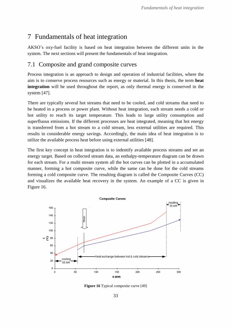
Fundamentals of heat integration
33
7 Fundamentals of heat integration
AKSO’s oxy-fuel facility is based on heat integration between the different units in the
system. The next sections will present the fundamentals of heat integration.
7.1 Composite and grand composite curves
Process integration is an approach to design and operation of industrial facilities, where the
aim is to conserve process resources such as energy or material. In this thesis, the term heat
integration will be used throughout the report, as only thermal energy is conserved in the
system [47].
There are typically several hot streams that need to be cooled, and cold streams that need to
be heated in a process or power plant. Without heat integration, each stream needs a cold or
hot utility to reach its target temperature. This leads to large utility consumption and
superfluous emissions. If the different processes are heat integrated, meaning that hot energy
is transferred from a hot stream to a cold stream, less external utilities are required. This
results in considerable energy savings. Accordingly, the main idea of heat integration is to
utilize the available process heat before using external utilities [48].
The first key concept in heat integration is to indentify available process streams and set an
energy target. Based on collected stream data, an enthalpy-temperature diagram can be drawn
for each stream. For a multi stream system all the hot curves can be plotted in a accumulated
manner, forming a hot composite curve, while the same can be done for the cold streams
forming a cold composite curve. The resulting diagram is called the Composite Curves (CC)
and visualizes the available heat recovery in the system. An example of a CC is given in
Figure 16.
Figure 16 Typical composite curve [49]

Fundamentals of heat integration
34
The overlap of the composite curves represents the possible energy recovery in the system,
i.e. the energy saved with heat integration. The point marked pinch denotes the pinch point in
the system. This point indicates the closest temperature approach in the system, ∆Tmin, which
is important as the external utilities requirements are dependent on ∆Tmin. A high value of
∆Tmin results in increased utility consumption. However, this is only true for a system with
both hot and cold utility requirements. If the system has only one utility requirement, reducing
the ∆Tmin would not lead to lower utility consumption. These types of systems are called
threshold systems.
Assuming that the system operates at steady-state and no external work is done by the system,
the energy balance for a stream undergoing a change from state 1 to state 2, can be expressed
as in Eq.Feil! Fant ikke referansekilden. If we further neglect changes in potential and
kinetic energy, assume constant Cp and assume the enthalpy to be only a function of
temperature, neglecting the pressure dependence, the expression can be simplified to Eq.(7.2).
2 2
2 12 1 2 1
2
V VQh h gz gz
m
(7.1)
2 1p p t sQ mC T T mC T T (7.2)
To visualize the required utilitiy levels in a system, the Grand Composite Curve (GCC) is an
important tool. The GCC plots shifted temperatures against net heat flow (Figure 17). The
shifted temperatures represent common temperatures for hot and cold streams, and are found
by reducing all hot stream temperatures by ∆Tmin/2, and increasing all cold temperature with
the same value. We can then plot a curve that gives us the net heat flow at various
temperatures in the process, relative to the pinch point [50].

Fundamentals of heat integration
35
Figure 17 Typical grand composite curve
The red circle points out the pinch point. The shaded area of the curve denotes the area where
heat can be exchanged between different temperature intervals. One of the “golden rules” in
pinch analysis is that one should never use external heating below pinch, or use external
cooling above pinch. Violating this rule will result in increased requirements of external
utilities. However an external heat source should not only be placed above pinch, but also
above the GCC. The curve is also used as a tool for selecting utilities, as it gives the required
temperature level for the external utility [48].
7.2 Steam generation
The steam generation in AKSO’s system is an important unit in the facility. The excess
energy in the flue gas is utilized to generate steam. In steam generation there exist three
different heat transfer zones. If starting from the lowest temperature, the water is preheater in
the economizer. The second zone is called the evaporator, where boiling at constant
temperature occurs. The last zone is the superheater, where steam is superheated to a specified
temperature [10]. A typical T-Q diagram for a HRSG is given in Figure 18.

Fundamentals of heat integration
36
Figure 18 T-Q diagram, for heat transfer in steam generation[10]
In a typical HRSG, the pinch point is located at the end point of the economizer, as can be
seen from Figure 18. However, for systems with a fired boiler, the pinch point might be
located at the cold end of the economizer. This is due to the large temperature difference
between the flue gas and the water. If this is the case, implementation of a BFW preheater is
common, as this will enable a greater steam generation.
If performing a heat balance over the evaporator and superheater, the steam production can be
expressed as:
, 1, 3,
1 3
flue p flue flue fluem c T Tm
h h
(7.3)
T1 is the temperature of the flue gas, at the inlet of the superheater. T3 is the temperature of
the flue gas at the outlet of the evaporator. h1and h3 are the enthalpy of water at the outlet of
the superheater and the economizer, respectively.
7.3 Intermediate Heat Carriers
Heat transfer between hot and cold streams can be done either directly or indirectly. If
transferred directly, one stream needs to be piped over to the other unit. Depending on the
fluid, the piping could be expensive or the pressure drop significant and. In addition direct
heat transfer might violate the safety regulations if the fluid is explosive, or if there is risk of
freeze-out. If this is the case indirect heating can be done by employing am intermediate Heat
Transfer Fluid (HTF). This matter is broadly applied to power plants but there exists only
limited research on the accurate use of intermediate heat carriers according to Smith [51].
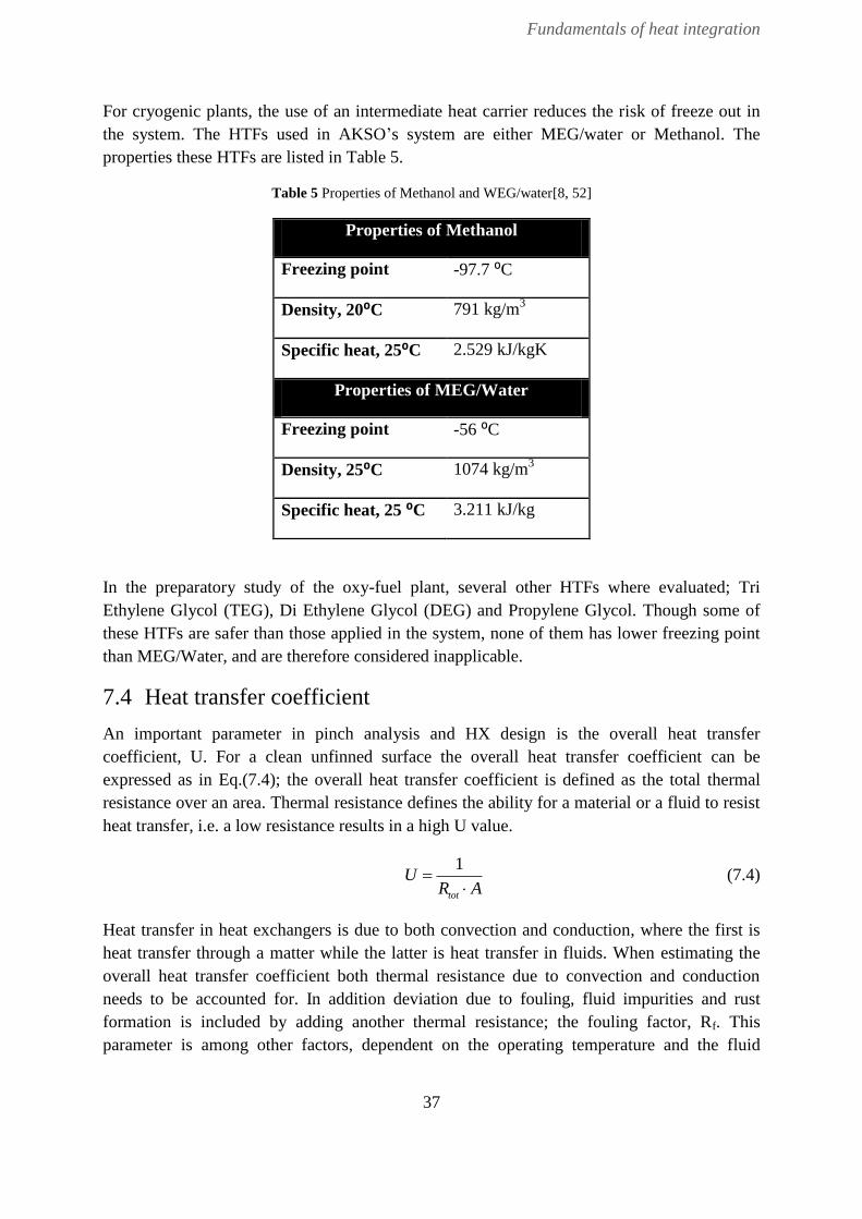
Fundamentals of heat integration
37
For cryogenic plants, the use of an intermediate heat carrier reduces the risk of freeze out in
the system. The HTFs used in AKSO’s system are either MEG/water or Methanol. The
properties these HTFs are listed in Table 5.
Table 5 Properties of Methanol and WEG/water[8, 52]
Properties of Methanol
Freezing point -97.7 ⁰C
Density, 20⁰C 791 kg/m3
Specific heat, 25⁰C 2.529 kJ/kgK
Properties of MEG/Water
Freezing point -56 ⁰C
Density, 25⁰C 1074 kg/m3
Specific heat, 25 ⁰C 3.211 kJ/kg
In the preparatory study of the oxy-fuel plant, several other HTFs where evaluated; Tri
Ethylene Glycol (TEG), Di Ethylene Glycol (DEG) and Propylene Glycol. Though some of
these HTFs are safer than those applied in the system, none of them has lower freezing point
than MEG/Water, and are therefore considered inapplicable.
7.4 Heat transfer coefficient
An important parameter in pinch analysis and HX design is the overall heat transfer
coefficient, U. For a clean unfinned surface the overall heat transfer coefficient can be
expressed as in Eq.(7.4); the overall heat transfer coefficient is defined as the total thermal
resistance over an area. Thermal resistance defines the ability for a material or a fluid to resist
heat transfer, i.e. a low resistance results in a high U value.
1
tot
UR A
(7.4)
Heat transfer in heat exchangers is due to both convection and conduction, where the first is
heat transfer through a matter while the latter is heat transfer in fluids. When estimating the
overall heat transfer coefficient both thermal resistance due to convection and conduction
needs to be accounted for. In addition deviation due to fouling, fluid impurities and rust
formation is included by adding another thermal resistance; the fouling factor, Rf. This
parameter is among other factors, dependent on the operating temperature and the fluid

Fundamentals of heat integration
38
velocity. If wall resistance is ignored the overall heat transfer coefficient may be expressed as
[53]:
1 1 1f
c h
R AU h h
(7.5)
Where 1/hh is the thermal heat resistance for the hot side of the HX and 1/hc is the thermal
heat resistances for the cold side of the HX. The heat transfer coefficient, h [W/m2K] depends
on conditions in the boundary layer, which again depend on the surface geometry, transport
properties and the fluid motion, i.e. laminar or turbulent flow. In addition the h-values will
change dynamically through a HX; the change is dependent on pressure, velocity and
temperature changes as well as possible phase transitions. Owing to the dependence on
numerous factors, the heat transfer coefficient is difficult to determine accurately [53, 54]. For
the purpose of this thesis the heat transfer coefficients used are extracted from literature,
giving only proposed values for shell and tube HXs. It is important to notice that using
tabulated values increase the error of estimation. All values used in this thesis, are extracted
from Table 2 “Typical film heat transfer coefficients for shell-and-tube heat exchangers” in
[55]. These values show that liquids tend to have a significantly higher h value than gases. For
the substances in this thesis (NG, water, CO2 and nitrogen) water has a considerable higher h-
value in liquid phase than both LNG and liquid CO2/N2. If LNG is assumed to only contain
light hydrocarbons, the proposed h-value lies between 1500-2000W/m2K. The tabulated h-
value for a CO2/N2 mixture in a gas phase is dependent on the pressure. Table 6 shows typical
values for gas2 at different pressures.
Table 6 Typical h-values for gas at different pressure [55]
Pressure [kPa] h [W/m2K]
100-200 80-125
1000 250-400
10 000 500-800
For the use of intermediate heat carrier, the relationship between the film heat transfer
coefficient and the contribution of ∆Ti for stream i can be related through Eq.(7.6). Where ∆Ti
is the individual temperature contribution for stream i, and C is a constant [56].
i
i
CT
h (7.6)
2 The values given apply to gases like: CO2, N2, air and light hydrocarbons mixtures.

Fundamentals of heat integration
39
As can be seen from Eq.(7.6), the temperature difference for stream i, is inversely
proportional to the square root of the heat transfer coefficient.
7.5 Area targeting
To optimize the heat integration done in a power plant, the total HX area should be examined,
as the cost of a HX increases with increasing area. For a single countercurrent heat exchanger,
the area is given by Eq.(7.7).
LM
QA
U T
(7.7)
Where Q [kW] is the duty of the heat exchanger U [kW/m2K] is the overall heat transfer
coefficient and ∆TLM [K] is the logarithmic mean temperature difference expressed as:
ln
H CLM
H
C
T TT
T
T
(7.8)
∆TH and ∆TC are the temperature differences at the hot and cold end of the HX, respectively.
In essence the surface area is approximately inversely proportional to the temperature
difference. In addition, the capital cost of a system is approximately proportional to surface
area, thus there exists a trade-off between CAPEX and energy costs when choosing ∆Tmin.
This is owing to the fact that the utility requirements increase with decreasing ∆Tmin, while the
opposite is true for the relationship between area of a HX and the value of ∆Tmin [48].

Simulation model and methodology
40

Simulation model and methodology
41
8 Simulation model and methodology
AKSO’s concept has been simulated to find possibilities of reducing the power consumption
in the system. In this chapter a description of the simulation model is given. The software
used for designing the model is presented, and the main specifications for the model are
given.
8.1 Simulation software
In this thesis Aspen Hysys Version7.2, is used as the simulation software. Aspen Hysys is a
process design environment, broadly used in the oil and gas industry. In Hysys, rigorous
steady-state and dynamic simulation models can be created. For the purpose of this thesis,
only steady-state simulation models have been employed. The simulation models are based on
flow diagrams provided by AKSO. In addition, an early stage simulation model created by
AKSO is used to extract data regarding the distillation column and the accurate fluid package.
8.2 Fluid packages
When predicting the state of gases and liquids at high pressure and low temperature, the ideal
gas law is not valid. In Hysys there exists different fluid packages, and choosing the right one
is critical to get accurate results. For the NG and the flue gas streams the Soave-Redlich-
Kwong (SRK) package is used. The SRK package contains binary interaction parameters for
all hydrocarbon-hydrocarbon pairs and is based on Van der Walls’ equation of state, Eq.(8.1)
This is a generalization of the ideal gas equation. The SRK equation of state is given by
Eq.(8.2) [57].
2
RT ap
v b v
(8.1)
RT ap
v b v v b
(8.2)
The SRK package would not give accurate results for the water/steam system. For this
purpose American Society of Mechanical Engineering (ASME) steam package is employed.
This package extracts data from the ASME 1967 steam tables. The limitations of ASME
steam are that a pressure below 1035 bar is required, and the temperature is limited to lie
between 0 and 816⁰C [58]. These limitations are acceptable for the purpose of this thesis.
8.2.1 Distillation column in Hysys
The distillation column in Hysys is the most complex unit operation, thus it needs to be
specially design to get accurate results. Among others the amount of stages, duty of the
reboiler/condenser and pressure drop specifications needs to be set. In addition initial
estimates need to be set for the column to converge to solution. This can, among others, be the
reflux ratio, the distillate flow or the bottom flow.

Simulation model and methodology
42
In Hysys the Francis Weir equation is used to calculate the liquid fraction leaving a stage[58].
1,5
N wL C l h (8.3)
Where LN is the liquid flowrate leaving tray N, ρ [kg/m3] is the density of liquid, lw is the weir
length and h is the height of liquid above weir. As calculation of a distillation column is
complex, the formulas used are of great importance. The vapor fraction leaving the tray is
calculated by:
vap frictionF k P (8.4)
Where F is the flowrate of vapor leaving tray N, k is the conductance and ∆Pfriction is the dry
hole pressure drop.
8.3 Process design and methodology
The simulation models are designed as stationary simulations files. The object of the
simulations is firstly to evaluate the heat integration in the original system. For this purpose, a
model using an oxygen stream with 0.95 mol% oxygen purity (case 1) is used. Thereby the
parameters upstream the oxy-burner is changed, and two new simulation models are created;
one with 0.90mol% oxygen purity (case 2) and one with 0.97mol% oxygen purity (case 3).
These models are used to find the impact on the CO2 CPU, by changing the oxygen purity.
The last simulation model is upgraded; the ASU is integrated and the selected oxygen purity,
and heat integration is employed. The process parameters used are based on the plant
specification for the proposed regasification plant from AKSO, which will be referred to as
the base case in the following. Some specifications were adjusted when needed. The main
simulation model is given in Appendix A. The overall assumptions for the simulation models
are listed below:
- No heat loss in any components (HXs, distillation column etc.)
- No heat loss in pipelines
- No pressure loss in pipelines
- Polytrophic efficiency of turbines is set to 80 %
- Adiabatic efficiency of compressors is set to 80%
- Polytrophic efficiency of pumps is set to 75%
- Pressure drop in cooler/heater is set to 30 kPa
- Intermediate heat carries are not included in the model
- Complete combustion is assumed in the burner
- All shell and tube heat exchangers works in a counter-current manner

Simulation model and methodology
43
- The duty of the distillation column is expected to be low compared to the other units
in the system, and are therefore neglected in the heat balance
8.3.1 Specifications of the LNG stream
The composition of the LNG feed is given in Table 7. The mass flow of LNG in the
simulation model, is specified to 44 790 kmol/h in accordance with AKSO’s utility flow
diagrams.
Table 7 Fuel composition
Component Chemical
symbol
Mole
fraction
Methane CH4 0.925
Ethan C2H6 0.055
Propane C3H8 0.010
Nitrogen N2 0.010
The LNG is pumped to 80 bar by two centrifugal pumps, before heated by five heat
exchangers, named LNG HX 1 – HX 5. The duties and pressure drop of all HXs are specified.
The pressure drop is set to 30 kPa. The duty for each HX is given in the Table 8, including the
fuel gas preheater, which preheats the NG routed to the oxy-burner.
Table 8 Duties of LNG heat exchangers
Unit Duty[MW]
LNG HX 1 4.1
LNG HX 2 2.3
LNG HX 3 28.2
LNG HX 4 63.3
LNG HX 5 59.7
Fuel gas preheater 0.5
After the last LNG HX, a tee is used to split the stream. 1.5 % of the NG is throttled to 250
kPa and heated, before routed to the oxy-fuel burner. The rest of the send-out gas is
transported to distributers. To identify which streams should be heat integrated, the heat
exchangers are not connected by energy streams in the models. This is done to give a higher
degree of freedom.

Simulation model and methodology
44
8.3.2 Specifications of the steam cycle
The steam cycle in the process has two purposes; generate power and produce steam. The
water goes in a cycle; after exiting the steam generation and power cycle, it is collected in a
drum and sent to condensate treatment. In the simulation model the dehydration is not
included, thus the water cycle is simulated as a single train. The mass flow of water in the
system is specified to 10 158 kmole/h, and the temperature and pressure prior the BFW pump
is specified to 25⁰C and 150 kPa.
The BFW is pumped to 5470 kPa, to give the accurate pressure upstream the steam boiler
(5450 kPa). The water is then preheated against flue gas in a shell and tube HX, where the
pressure drop is specified to 20 kPa and the outlet temperature is specified to 155⁰C.The
steam boiler is simulated as a separator and a HX, as there is no accurate unit operator
available in Hysys. Steamboiler_1 and steam_boiler_2 are connected by an energy stream, as
can be seen in Figure 19. The duty of the steam boiler is specified to 107.2 MW. The shell
and tube HX is simulated with weighted HX design to get the accurate T-H profile. In
weighted design, the heating curve is broken into intervals. This is applied to all shell and
tube heat exchangers in the simulation models.
Figure 19 Simulation model of steam boiler
Liquid water exits the bottom of the steam boiler, while steam is drawn-off at the top of the
column, where the temperature is specified to 251.9⁰C. Steam is then superheated against
flue gas, where the outlet pressure from the MP superheater is set to 4091 kPa. The liquid
water is routed to the collection drum, while the superheated steam is sent to the MP turbine,
where the outlet pressure is specified to 500 kPa. LP steam is drawn-off to vaporize LNG
(LNG heater 5), and preheat oxygen and fuel prior to the combustion. Approximately 55 % of
the steam from the MP turbine is routed to the LP turbine where the outlet pressure is
specified to 14 kPa. The steam condensate from the LP turbine is cooled by vaporizing LNG
(LNG heater 4) before routed to the collection drum. The oxygen and fuel gas preheater is
simulated as one HX, owing to lack of specifications in the flow sheets. In addition the duties
Stem
boiler_1
Stem
Boiler_2
Flue gas
BFW
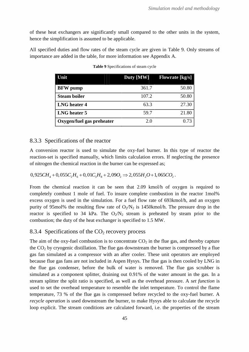
Simulation model and methodology
45
of these heat exchangers are significantly small compared to the other units in the system,
hence the simplification is assumed to be applicable.
All specified duties and flow rates of the steam cycle are given in Table 9. Only streams of
importance are added in the table, for more information see Appendix A.
Table 9 Specifications of steam cycle
Unit Duty [MW] Flowrate [kg/s]
BFW pump 361.7 50.80
Steam boiler 107.2 50.80
LNG heater 4 63.3 27.30
LNG heater 5 59.7 21.80
Oxygen/fuel gas preheater 2.0 0.73
8.3.3 Specifications of the reactor
A conversion reactor is used to simulate the oxy-fuel burner. In this type of reactor the
reaction-set is specified manually, which limits calculation errors. If neglecting the presence
of nitrogen the chemical reaction in the burner can be expressed as;
4 2 6 3 8 2 2 20,925 0,055 0,01 2,09 2,055 1,065CH C H C H O H O CO .
From the chemical reaction it can be seen that 2.09 kmol/h of oxygen is required to
completely combust 1 mole of fuel. To insure complete combustion in the reactor 1mol%
excess oxygen is used in the simulation. For a fuel flow rate of 693kmol/h, and an oxygen
purity of 95mol% the resulting flow rate of O2/N2 is 1450kmol/h. The pressure drop in the
reactor is specified to 34 kPa. The O2/N2 stream is preheated by steam prior to the
combustion; the duty of the heat exchanger is specified to 1.5 MW.
8.3.4 Specifications of the CO2 recovery process
The aim of the oxy-fuel combustion is to concentrate CO2 in the flue gas, and thereby capture
the CO2 by cryogenic distillation. The flue gas downstream the burner is compressed by a flue
gas fan simulated as a compressor with an after cooler. These unit operators are employed
because flue gas fans are not included in Aspen Hysys. The flue gas is then cooled by LNG in
the flue gas condenser, before the bulk of water is removed. The flue gas scrubber is
simulated as a component splitter, draining out 0.91% of the water amount in the gas. In a
stream splitter the split ratio is specified, as well as the overhead pressure. A set function is
used to set the overhead temperature to resemble the inlet temperature. To control the flame
temperature, 73 % of the flue gas is compressed before recycled to the oxy-fuel burner. A
recycle operation is used downstream the burner, to make Hysys able to calculate the recycle
loop explicit. The stream conditions are calculated forward, i.e. the properties of the stream
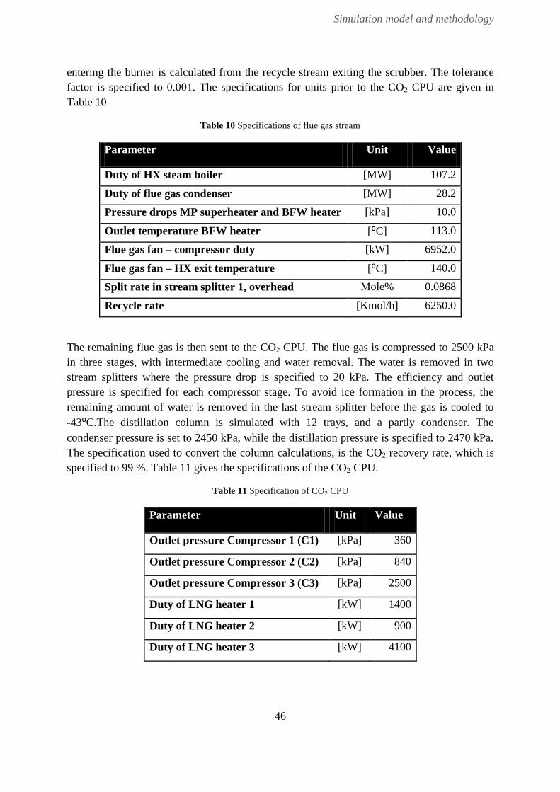
Simulation model and methodology
46
entering the burner is calculated from the recycle stream exiting the scrubber. The tolerance
factor is specified to 0.001. The specifications for units prior to the CO2 CPU are given in
Table 10.
Table 10 Specifications of flue gas stream
Parameter Unit Value
Duty of HX steam boiler [MW] 107.2
Duty of flue gas condenser [MW] 28.2
Pressure drops MP superheater and BFW heater [kPa] 10.0
Outlet temperature BFW heater [⁰C] 113.0
Flue gas fan – compressor duty [kW] 6952.0
Flue gas fan – HX exit temperature [⁰C] 140.0
Split rate in stream splitter 1, overhead Mole% 0.0868
Recycle rate [Kmol/h] 6250.0
The remaining flue gas is then sent to the CO2 CPU. The flue gas is compressed to 2500 kPa
in three stages, with intermediate cooling and water removal. The water is removed in two
stream splitters where the pressure drop is specified to 20 kPa. The efficiency and outlet
pressure is specified for each compressor stage. To avoid ice formation in the process, the
remaining amount of water is removed in the last stream splitter before the gas is cooled to
-43⁰C.The distillation column is simulated with 12 trays, and a partly condenser. The
condenser pressure is set to 2450 kPa, while the distillation pressure is specified to 2470 kPa.
The specification used to convert the column calculations, is the CO2 recovery rate, which is
specified to 99 %. Table 11 gives the specifications of the CO2 CPU.
Table 11 Specification of CO2 CPU
Parameter Unit Value
Outlet pressure Compressor 1 (C1) [kPa] 360
Outlet pressure Compressor 2 (C2) [kPa] 840
Outlet pressure Compressor 3 (C3) [kPa] 2500
Duty of LNG heater 1 [kW] 1400
Duty of LNG heater 2 [kW] 900
Duty of LNG heater 3 [kW] 4100

Simulation model and methodology
47
8.4 Results and discussion
In this section the resulting temperatures and duties from the main simulation model (Case 1)
are presented and discussed. For further details see Appendix A.
8.4.1 LNG stream
For the base case the inlet temperature of LNG HX 1 was calculated to -160.3⁰C. This is
equivalent with the result from the simulations. The last heat exchanger (LNG HX 5) heats
the gas to 3.9 ⁰C, which is lower than expected. In AKSO’s flow sheets the temperature is
calculated to 8.7 ⁰C. Getting the accurate outlet temperature would require increasing the duty
of LNG HX 5 to 63 MW. However, the low temperature could be caused by the selected fluid
package, other program specifications or due to the design of the HX in the base case: The
system used a special water bath technology for LNG HXs 4-5. There were not done any
changes to gain a higher temperature. In accordance with Hans Kristian Rusten from AKSO,
the temperature was decided to be acceptable for the purpose of this thesis. The exit
temperatures of the LNG HXs, LNG pumps and the fuel gas preheater are given in Table 12.
Table 12 Exit temperatures of LNG HXs
Unit Texit [⁰C]
LNG pump 1 -162.30
LNG pump 2 -160.30
LNG HX 1 -154.60
LNG HX 2 -151.40
LNG HX 3 -114.10
LNG HX 4 -56.80
LNG HX 5 3.92
Fuel gas preheater 26.96
The simulation model shows that the LNG is vaporized and heated transcritical, i.e. above the
phase envelope. In subcritical vaporization the fluid evaporates at nearly constant
temperature, resulting in a flat T-H profile. In transcritical vaporization a steeper gradient is
experienced, as can be seen from Figure 20, which shows the T-H profile of LNG HX 4.

Simulation model and methodology
48
Figure 20 T-H profile of LNG HX 4
8.4.2 Steam cycle
The simulation model shows that water exits the BFW heater as compressed liquid water at
5450 kPa. The steam boiler overhead pressure was calculated to 4107 kPa, giving a vapor
molar flow of 9955 kmol/h. This resembles the molar flow calculation in the base case, which
is important as the correct amount of steam is required to get the accurate turbine yield. MP
steam is than superheated to 398.1⁰C, against flue gas from the oxy-fuel boiler. The
temperature is 2⁰C lower than expected, which is acceptable. The LP steam used to heat LNG
(LNG heater 5) oxygen and fuel gas, is split into two streams; one going to the LNG heater,
while the rest is routed to the oxygen/fuel gas preheater. The split rate was adjusted from 98.6
% going to the LNG heater to 97 %, due to freeze out in the oxygen/fuel preheater. With these
flow rates the LP steam is condensed and super cooled in both HXs. The vapor fraction of the
steam condensate leaving the LP turbine was calculated to 0.8938 and the steam condensate is
liquefied and supercooled in LNG heater 4. The exit temperatures of LNG heater 4 and LNG
heater 5 are lower than expected. As already mentioned these HXs use a water bath
technology. As these HXs are simulated as ordinary heaters this could be the reason for the
low temperatures. If the results from the simulation model are correct, the water flow should
be increased to gain a higher outlet temperature.
Duties, start temperatures (Ts), target temperatures (Tt), inlet and outlet pressure for each unit
is given in Table 13.

Simulation model and methodology
49
Table 13 Output parameters for steam cycle
Unit Ts
[⁰C]
Tt
[⁰C]
Inlet
pressure
[kPa]
Oulet
pressure
[kPa]
Duty
[MW]
BFW pump 25.0 25.5 150 5470 361.7
BFW heater 25.5 155.0 5470 5450 27.7
Steam boiler 155.0 251.9 5450 4107 107.2
MP superheater 251.9 396.6 4107 4091 20.3
MP turbine 396.6 174.6 4091 500 20.3
LP Turbine 174.6 52.7 500 14 12.5
LNG heater 4 52.7 5.3 14 13 63.3
LNG heater 5 52.7
..7
15.4 500 470 59.7
O2/fuel gas
preheater
52.7 10.5 500
470 2.0
The pressure drop in the steam boiler is significantly high. However, it matches the pressure
drop in the base case, and is therefore considered applicable. The pressure drop in LNG heater
4 was set to 1 kPa. This HX operates under vacuum conditions, and the accurate pressure drop
is not given in AKSO’s flow sheets. As the selected pressure drop has no impact on the
evaluation of the heat integration in the system, it is assumed to be acceptable. A schematic of
the power generation and the LP steam consumption is given in Figure 21.
Figure 21 Power and steam cycle
8.4.3 CO2 CPU
The reaction balance of the oxy- burner is given in the Table 14. As can be seen from the
table the carbon and hydrogen in the fuel is completely converted to CO2 and water. However,

Simulation model and methodology
50
it is important to notice that this would not be the case in a real combustion, as the flue gas
would contain impurities like NOx and CO as discussed in Chapter 3.
Table 14 Reaction balance for the oxy-burner
Component Total inflow Total reaction Total
outflow
Methane 641
641 0
Ethane 38
38 0
Propane 6.9
6.9 0
H2O 118 1424 1542
Oxygen 1557
1450 106.9
Nitrogen 700
0 700
CO2 5422 738.1 6160
The composition of the oxygen stream is adjusted from that given in the flowsheets from
AKSO. The oxygen stream contained 95mol%, 4mol% N2 and 1mol% CO2, originally. In the
simulation model the CO2 content is neglected in accordance with PhD student Fu Chao. For
a real process, argon would probably be present in the oxygen stream. In this simulation
model however, argon is not included owing to the specifications given in AKSO’s flow
sheets. The oxygen stream used in this model contains 95mol% oxygen and 5mol% nitrogen.
With the specified recycle rate, O2/N2 flow and fuel composition, the composition of the flue
gas is as given in Table 15. The flue gas composition obtained in Hysys resembles that of
AKSO. The flue gas flow was calculated to 8509 kmol/h.
Table 15 Flue gas composition
Component Mole fraction in
flue gas
Mole fraction
after recycling
H2O 0.180 0.019
Oxygen 0.013 0.015
Nitrogen 0.082 0.099
CO2 0.724 0.880
The specified recycle rate of 6250 kmol/h, results in a flame temperature of 1448⁰C. This
result is satisfactory, as the temperature should be below 1450 ⁰C according to AKSO. The
duty of the flue gas fan was calculated to 11.5 MW. This result differs from the base case
mainly because of the selected unit operators employed. All resulting duties, temperatures and
pressures for the CO2 CPU are given in Table 16.

Simulation model and methodology
51
Table 16 Output parameters for the CO2 CPU
Unit Ts
[⁰C]
Tt
[⁰C]
Inlet
pressure
[kPa]
Outlet
pressure
[kPa]
Duty
[MW]
MP superheater 1448.0 1292.0 101.0 91.0 20.4
Steam Boiler 1292.0 393.8 91.0 81.0 107.2
BFW heater 393.8 113.0 81.0 71.0 27.7
Flue gas fan 113.0 140.0 71.0 130.4 11.5
Flue gas cond. 140.0 18.6 130.4 100.4 28.2
Recycle Comp. 18.6 44.6 100.4 135.0 1.7
Compressor 1 18.6 142.2 100.4 360.0 1.1
HX1 142.2 8.2 360.0 330.0 1.4
Compressor 2 8.2 100.3 310.0 840.0 0.8
HX2 100.3 2.9 840.0 810.0 0.9
Compressor 3 2.9 110.2 790.0
.0
2500.0 0.9
HX3 110.2 -42.0 2500.0 2470.0 4.1
The distillation column was converged with a CO2 capture rate at 99 %, the weighted error
was calculated to 0,000. The duty of the condenser was calculated to 230 kW. The molar
flow going to CO2 storage was calculated to 751.5kmol/h with a CO2 concentration of 0,972
mol%. A schematic of the CO2 CPU in Hysys is given in Figure 22.
Figure 22 CO2 separation and compression
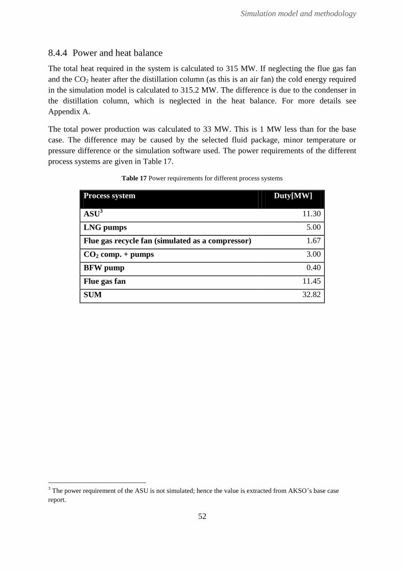
Simulation model and methodology
52
8.4.4 Power and heat balance
The total heat required in the system is calculated to 315 MW. If neglecting the flue gas fan
and the CO2 heater after the distillation column (as this is an air fan) the cold energy required
in the simulation model is calculated to 315.2 MW. The difference is due to the condenser in
the distillation column, which is neglected in the heat balance. For more details see
Appendix A.
The total power production was calculated to 33 MW. This is 1 MW less than for the base
case. The difference may be caused by the selected fluid package, minor temperature or
pressure difference or the simulation software used. The power requirements of the different
process systems are given in Table 17.
Table 17 Power requirements for different process systems
Process system Duty[MW]
ASU3 11.30
LNG pumps 5.00
Flue gas recycle fan (simulated as a compressor) 1.67
CO2 comp. + pumps 3.00
BFW pump 0.40
Flue gas fan 11.45
SUM 32.82
3 The power requirement of the ASU is not simulated; hence the value is extracted from AKSO’s base case
report.
Evaluation of existing heat integration in the system
53
9 Evaluation of existing heat integration in the system
The evaluation of the existing heat integration in the system is based on the simulation results
from Chapter 8. The objective of this chapter is to evaluate the proposed heat integration in
the base case and identify possibilities of power reduction in the plant.
9.1 Methodology
A simplified schematic of the heat integration in the base case can be seen in Figure 1. A
procedure is established to identify the heat integration in the systems, and thereby evaluate it.
Firstly the hot and cold streams are extracted from the simulation model. Only streams of
interest to the heat integration are accounted for. The hot and cold streams are drawn
separately in a T-Q diagram to evaluate the sequence of the pair matching in the system. For
heat exchangers using intermediate heat carriers, the placement of the intermediate HTFs are
evaluated, based on individual heat transfer coefficients. The utility consumption is evaluated
by using the CC and GCC for the system. The assumptions made in Chapter 8 still apply, in
addition the following is assumed:
- Heat losses are not taken into account
- The condenser in the distillation column is not taken into account in the heat balance
as the duty is lower than 1MW.
- The flue gas fan HX is not taken into account in the heat integration.
The CC and the GCC are drawn using PRO_PI, which is an add-in to Microsoft Excel,
developed by Industriell Energianalys AB at Chalmers Industriteknik in Sweden. The
program draw the curves based on start/target temperatures and duties.
9.2 Data extraction
To be able to evaluate the heat integration in the process, hot and cold streams needs to be
identified. The system is divided into three main units; the regasification unit, the steam cycle
and the CO2 CPU. The different stream data are extracted from the main simulation file. A
stream is identified as a mass flow with a given pressure, i.e. a new stream is defined
whenever the pressure or the flow rate of the stream changes. Exception is made for the steam
boiler, see Section 9.2.1.
9.2.1 Steam cycle
The steam cycle are divided into one cold stream and three hot streams. The cold stream is the
preheating of BFW and the steam generation. The hot streams are defined as the streams
going through LNG heater 5, LNG heater 4 and the oxygen/fuel preheater. In the following
the cold stream is named C2 while the hot streams are named H1-H3 as can be seen from
Figure 23.
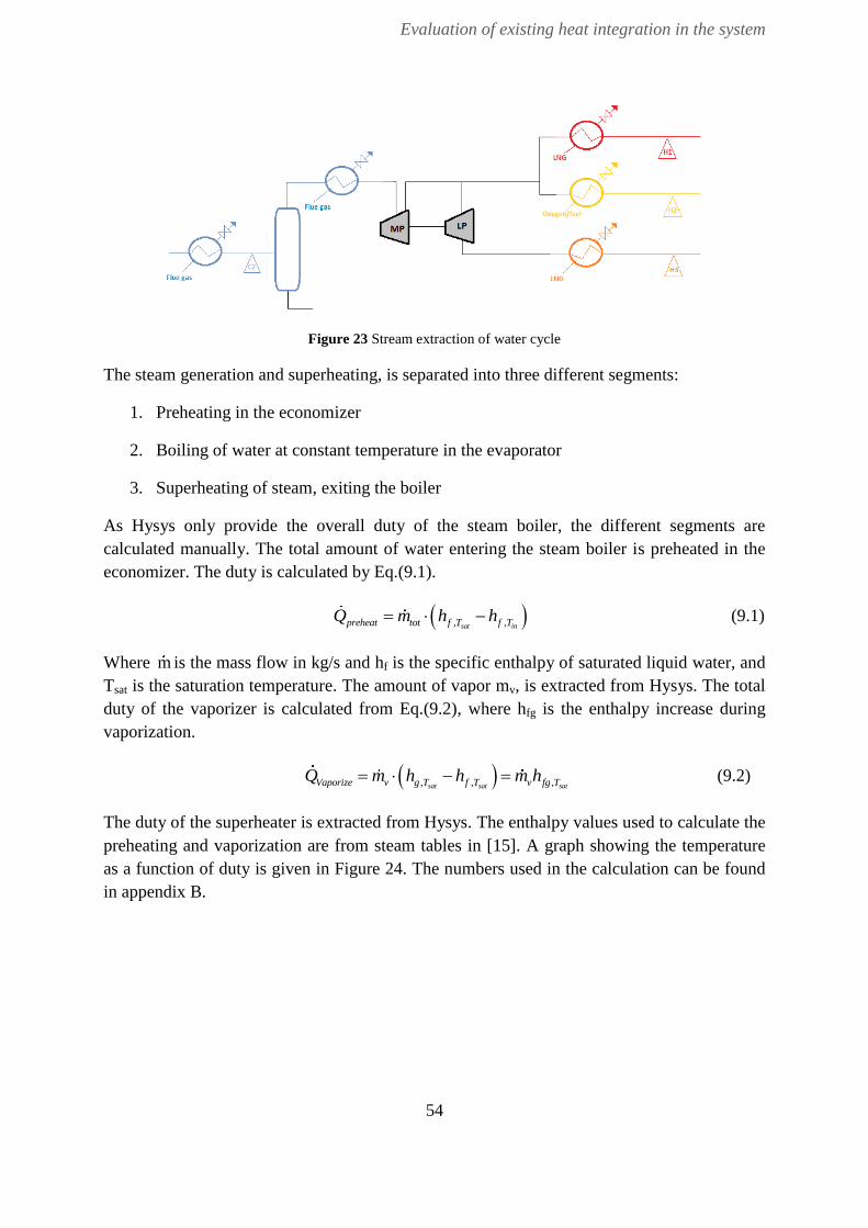
Evaluation of existing heat integration in the system
54
Figure 23 Stream extraction of water cycle
The steam generation and superheating, is separated into three different segments:
1. Preheating in the economizer
2. Boiling of water at constant temperature in the evaporator
3. Superheating of steam, exiting the boiler
As Hysys only provide the overall duty of the steam boiler, the different segments are
calculated manually. The total amount of water entering the steam boiler is preheated in the
economizer. The duty is calculated by Eq.(9.1).
, ,sat inpreheat tot f T f TQ m h h (9.1)
Where m is the mass flow in kg/s and hf is the specific enthalpy of saturated liquid water, and
Tsat is the saturation temperature. The amount of vapor mv, is extracted from Hysys. The total
duty of the vaporizer is calculated from Eq.(9.2), where hfg is the enthalpy increase during
vaporization.
, , ,sat sat satVaporize v g T f T v fg TQ m h h m h (9.2)
The duty of the superheater is extracted from Hysys. The enthalpy values used to calculate the
preheating and vaporization are from steam tables in [15]. A graph showing the temperature
as a function of duty is given in Figure 24. The numbers used in the calculation can be found
in appendix B.

Evaluation of existing heat integration in the system
55
Figure 24 T-H diagram steam boiler
The stream data are given in Table 18. The flow rate of C2 change in the boiler as liquid is
drawn-off at the bottom of the vessel. All data is extracted from the simulation model in
Hysys, which is equivalent to the information given in Chapter 8.
Table 18 Stream data for water cycle
Stream Flowrate
[kmol/h]
Tstart
[⁰C]
Ttarget
[⁰C]
Duty
[MW]
C2 10160 25.53 398.3 155.4
H1 4361 174.60 16.4 59.7
H2 145 174.60 11.4 2.0
H3 5450 52.58 5.7 63.3
9.2.2 LNG and flue gas streams
The LNG train is identified as one cold stream. The total duty calculated to 157.7 MW. The
stream will be referred to as C1 in the following chapters. The flue gas is divided into four
different hot streams, where change in mass flow or pressure defines a new stream. The
streams are named H4 – H8. The stream data for the hot streams is given in Table 19.
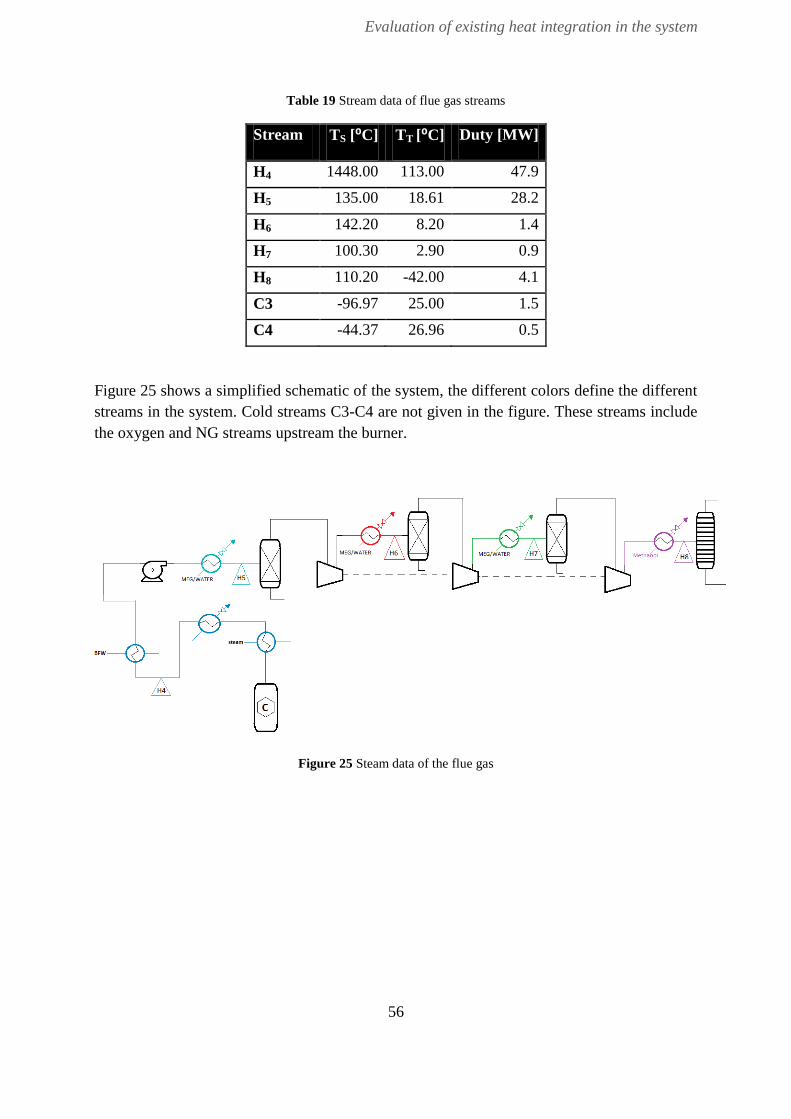
Evaluation of existing heat integration in the system
56
Table 19 Stream data of flue gas streams
Stream TS [⁰C] TT [⁰C] Duty [MW]
H4 1448.00 113.00 47.9
H5 135.00 18.61 28.2
H6 142.20 8.20 1.4
H7 100.30 2.90 0.9
H8 110.20 -42.00 4.1
C3 -96.97 25.00 1.5
C4 -44.37 26.96 0.5
Figure 25 shows a simplified schematic of the system, the different colors define the different
streams in the system. Cold streams C3-C4 are not given in the figure. These streams include
the oxygen and NG streams upstream the burner.
Figure 25 Steam data of the flue gas

Evaluation of existing heat integration in the system
57
9.3 Results and discussion
The objective of the evaluation is to investigate if the heat integration in the base case can be
improved. The heat integration is evaluated in terms of sequence of the stream pairing and
placement of HTFs. All stream data used are extracted from the previous chapter.
9.3.1 Composite curves for the system
Before evaluating the heat integration in the system, the CC is drawn to visualize the overall
temperature-heat content in the system. The steam consumption is not taken into account
when drawing the CC, as LP steam is considered an external utility. It can be discussed
whether the steam condensate is an external utility. In this thesis cooling of steam condensate
is viewed upon as part of the system, and is therefore not considered to be an external utility.
The CC for case 1 is given in Figure 26. The input data used to draw the curves can be found
in Appendix C.
Figure 26 CC for the base case
The composite curve for the system indicates that no external cooling is required, which
makes the system a threshold problem, hence shifting the ∆Tmin will not reduce the utility
requirements. The pinch point in the system is in the cold end of the CC. The cold pinch
temperature is calculated to -160.3 ⁰C, and a hot pinch temperature of -43⁰C resulting in a
∆Tmin > 110⁰C.
9.3.2 Sequence of the streams
The streams extracted from the simulation file, are drawn in a T-Q diagram (Figure 27). As it
exist a trade-off between ∆T in and the required heat transfer area, the heat transfer sequence
in the plant, should follow logically from temperatures. The logarithmic mean temperature
difference is used to select the sequence of the streams.
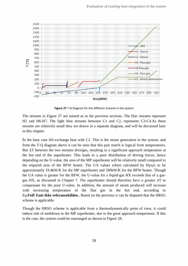
Evaluation of existing heat integration in the system
58
Figure 27 T-Q Diagram for the different streams in the system
The streams in Figure 27 are named as in the previous sections. The lilac streams represent
H2 and H6-H7. The light blue streams between C1 and C2, represents C3-C4.As these
streams are relatively small they are drawn in a separate diagram, and will be discussed later
in this chapter.
In the base case H4 exchange heat with C2. This is the steam generation in the system, and
from the T-Q diagram above it can be seen that this pair match is logical from temperatures.
But ∆T between the two streams diverges, resulting in a significant approach temperature at
the hot end of the superheater. This leads to a poor distribution of driving forces, hence
depending on the U-value, the area of the MP superheater will be relatively small compared to
the required area of the BFW heater. The UA values where calculated by Hysys to be
approximately 19.4kW/K for the MP superheater and 180kW/K for the BFW heater. Though
the UA value is greater for the BFW, the U-value for a liquid-gas HX exceeds that of a gas-
gas HX, as discussed in Chapter 7. The superheater should therefore have a greater ∆T to
compensate for the poor U-value. In addition, the amount of steam produced will increase
with increasing temperature of the flue gas in the hot end, according to
Eq.Feil! Fant ikke referansekilden.. Based on the previous it can be disputed that the HRSG
scheme is applicable.
Though the HRSG scheme is applicable from a thermodynamically point of view, it could
induce risk of meltdown in the MP superheater, due to the great approach temperature. If this
is the case, the system could be rearranged as shown in Figure 28.

Evaluation of existing heat integration in the system
59
Figure 28 Different boiler scheme
In Figure 28 the superheater is shifted to a lower temperature, while the evaporator is shifted
to a higher temperature to reduce risk of meltdown. As the h-value of water is greater than
that of steam, the conduction through the material will increase, which will result in less risk
of meltdown. However, the area of the MP superheater will increase, as ∆T is reduced. The
size of the boiler could however, be reduced as the driving forces are increased in the
evaporator. If this scheme will improve the HRSG is dependent on expenses and safety
regulations, and will not be further discussed in this thesis.
From Figure 27 it is difficult to evaluate the sequence of H2, H6-H7 and C3-C4 Therefore a
separate graph is made, omitting the steam generation. The graph is given in Figure 29.

Evaluation of existing heat integration in the system
60
Figure 29 T – Q Diagram omitting H4 and C2
Figure 29 shows the streams drawn logically from LMTD. The colors indicate which hot
streams heat exchange with the different temperature intervals for C1, C3 andC4 in the base
case (E.g. the hot streams heating LNG from -160.3 to -114 are colored dark red). Though the
target temperature for H6-H7 exceeds that of H3 the difference are insignificant making the
stream matches acceptable. This is also valid for the other streams in the graph.
Hot stream H1 is LP steam. Reducing the use of LP steam in the system would lead to
increased power production. The GCC for the system can be used as a tool to target the
required utility level. To minimize the energy cost in the plant the use of expensive utility
levels should be minimized. In the base case only LP steam is used in the power and steam
plant, while Cooling Water (CW) is used in the ASU. The GCC for case 1 is given in Figure
30. The curve is drawn with a ∆T = 30K. As can be seen from the graph only a low level
utility is required in the system. The required amout of utility is calculated to 61.7 MW. The
input data used to calcualted to GCC is given in Appendix C.
H8
H3
H7
H6
H2
H5
H1
C3/C4
4C4

Evaluation of existing heat integration in the system
61
Figure 30 GCC for the base case
From a thermodynamic point of view CW could be used instead of steam. However, this
would require significant amounts of water to prevent freeze-out in the system, thus this
would require implementation of a vast water system. The water needs to be purified and
chlorinated, which would make the system more climate sensitive and less environmental
friendly.Another possible solution is to lower the LP steam production and increase the duty
of the steam condenser, which would result in increased power production in the LP turbine.
In the main simulation model the molar flow of LP steam is set to 4506 kmol/h, and the
power production in the LP steam turbine is calculated to 12.52 MW. If reducing the LP
production to 3704 kmol/h and the duty of LNG heater 5 with 10 MW, the power production
in the LP steam turbine is incrased with 1.35 MW. However, the outlet temperature of LNG
heater 4 is reduced to approximately 1⁰C, which incrase the risk of freeze-out in the system.
9.4 Placement of HTFs
For stream H5 – H8 HTFs either MEG/water or Methanol are used as heat transfer fluids. The
placement of the HTFs is important to the heat exchanger design, as explained in Chapter 7.
To determine the accurate temperature level for the intermediate heat carrier, according to
Eq.(7.6), an estimated h-value for the different streams is required. For LNG an average value
is used; 1750 W/m2K. For the hot streams H5-H6, the h-value is dependent on the pressure of
the streams. The h-values chosen are average values of tabulated h-values for gas, given in
Chapter7.4. Table 20 gives the chosen values.

Evaluation of existing heat integration in the system
62
Table 20 Chosen h-values for the hot streams in the system
Stream Chosen h [W/m2K]
H5 103
H6 103
H7 325
H8 325
As the film transfer coefficient on the hot side of all HXs, using HTFs are much lower than
that of LNG; the chosen individual ∆Ti should be higher than that of the cold stream. It two
streams (i and j) should experience the same heat transfer area the following should apply:
i i j jh T h T (9.3)
This equation is derivate from Eq.(7.6), where ∆T is inversely proportional to the square root
of the h-value. It is important to notice that increasing the magnitude of the h-value by 100
will only decrease ∆T by 10. In the following the placement of the HTF in the different HXs
will be discussed.
9.4.1 Placement of HTF in LNG HX 1
In the first LNG HX Methanol is employed as the HTF.. The heat carrier extracts and emits
heat at the same temperature level, as can be seen from Figure 31. LNG is heated to
approximately -155⁰C, by cooling flue gas prior to the distillation column (LNG heater 3).
Figure 31 Placement of HTF in LNG HX 1
Figure 31shows that the HFT is placed closest to the hot stream. The h-value of the hot stream
is estimated to 325 W/m2K, while the h-value for LNG is estimated to be 1750 W/m
2K. The
square root of these h-values is 18 and 42, respectively. This means that the temperature
approach between the hot stream and the HTF should be twice that of the LNG and the HTF,
(Eq.(9.3)). As can be seen from Figure 31, this is not valid for. As already discussed the HTF

Evaluation of existing heat integration in the system
63
should approach the LNG from a thermodynamic point of view. However, it is important to
avoid freeze-out in the system. The cold temperature of Methanol in the system is -60⁰C,
while the freezing point of Methanol is -97.7⁰C according to Table 5.
9.4.2 Placement of HTF in LNG HX 2 and LNG HX3
In LNG HX 2 WEG/water is used. The HTF firstly heats the LNG, before it is split into two
streams, one going LNG heater 1 and one going to LNG heater 2, as can be seen from Figure
32. In LNG HX3 the same HTF is applied and placement of the HTF coincides with that of
LNG HX 2, hence only the placement of the HTF in LNG HX 2 is discussed.
Figure 32 MEG/Water cycle
Figure 33 shows the placement of the HTF. The HTF emits heat at 25⁰C and extracts heat at
-30⁰C. After heating the LNG, 60 % of the HTF is routed to LNG heater 1. From the graph to
the left it can be seen that the HFT is placed close to the hot fluid. The same is valid for LNG
heater 2. As already discussed, the HTF should be place closest to the fluid possessing the
greater h-value, in this case the LNG. However, safety needs to be taken into consideration.
For all HXs using HTFs, AKSO has chosen to place the HFT at least 25⁰C above its freezing
point. This is done to prevent freeze-out in the system. As the freezing point of MEG/Water
is -56⁰C, the HTF cannot be shifted closer to the LNG. However, it could be beneficial to
choose another HTF. If using Methanol instead, the HTF could be shifted closer to the LNG
as can be seen in the graph at the right. This would increase the temperature difference in
LNG heaters 1-2. However, it is important to notice that the selection of HTFs is dependent
on several factors. The density is higher for MEG/Water then for Methanol; hence the pipe
diameter can be reduced if employing MEG/Water as the HTF. In addition, the heat capacity
is greater for MEG/Water compared to Methanol. I.e. a smaller ∆T is experienced using
MEG/Water if the duty is held constant. In addition, the expenses of using Methanol instead
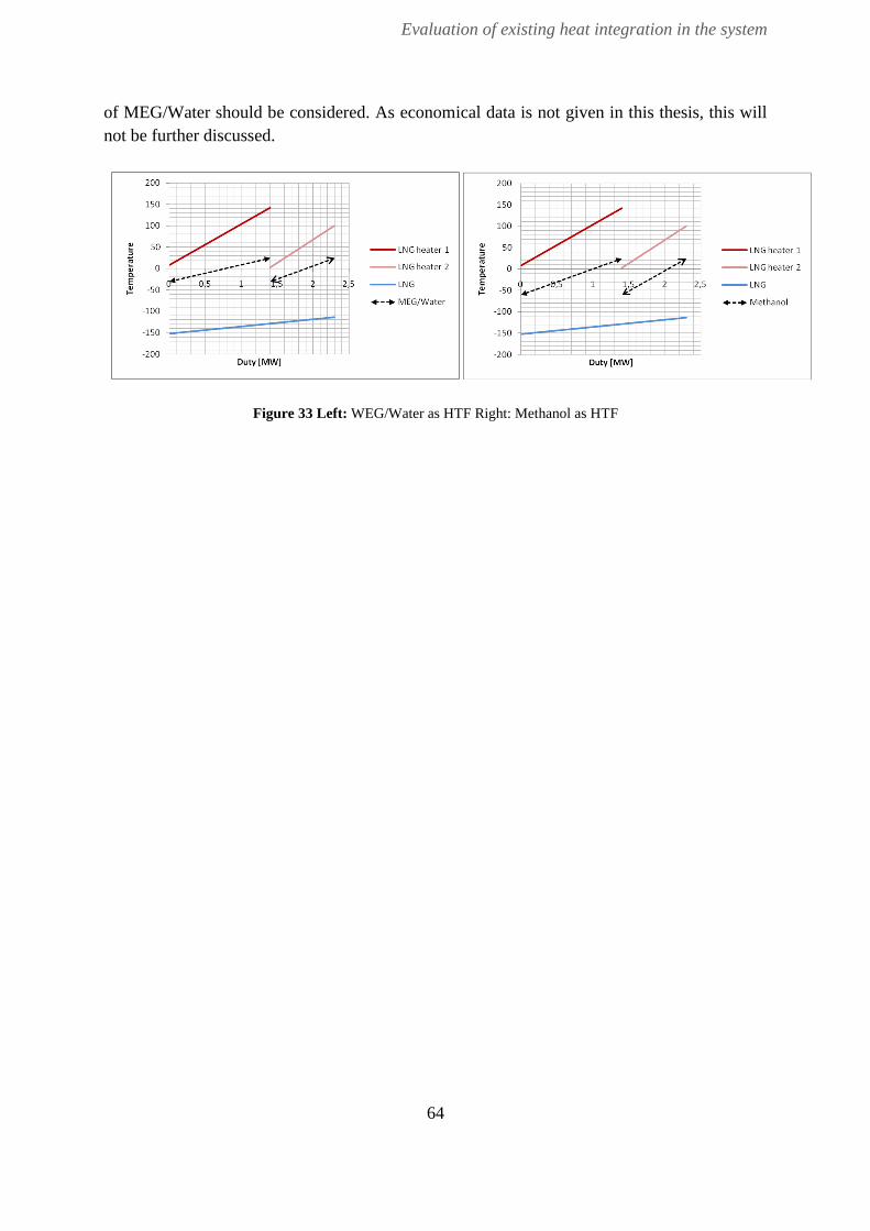
Evaluation of existing heat integration in the system
64
of MEG/Water should be considered. As economical data is not given in this thesis, this will
not be further discussed.
Figure 33 Left: WEG/Water as HTF Right: Methanol as HTF

Different oxygen purities
65
10 Different oxygen purities
Different oxygen purities where tested to find the impact on the CO2 CPU. Three different
purity levels were evaluated; 90, 95 and 97mol%.For the main simulation model the molar
flow of O2/N2 were set to 1540 kmol/h. When simulating the process with different oxygen
purity, the molar flow rate of O2/N2 was adjusted to maintain 1mole% excess oxygen in the
feed. The molar flow is calculated from the flow rate in case1:
97 97 95 95 90 90n x n x n x (10.1)
Where n is the molar flow of O2/N2, and x is the molar fraction of oxygen.
To give a complete evaluation the simulation model needs to be specially designed for each
case, to simplify the problem some variables are kept constant in the different cases;
- All duties of heater/coolers in the purification unit are held constant, e.g. temperatures
are expected to change with oxygen purity.
- The recycle rate is held constant.
- The distillation column is converged to give the same CO2 recovery rate for the
different cases, as a specified recovery rate is required for transportation and storage
of CO2. The CO2 recovery rate is defined as the fraction of CO2 captured from the
formed CO2 in the combustion.
- The duty of the flue gas fan is not taken into account when comparing the different
cases, owing to the fact that a different operator is used in the simulations.
- In addition the ASU is not simulated; hence, only the power consumption of the CO2
CPU is calculated for the different cases. Though the ASU is not simulated, the trade-
off between power savings in the CO2 CPU and the ASU is discussed.
With the previous assumptions the different cases are evaluated in terms of:
1. Compression work in the CO2 purification unit
2. Duty of distillation column
3. Overall power consumption
10.1 Case studies
Three different case studies were investigated. For case 1 the oxygen purity is specified to 95
mol%. The results from this case study resemble those given in Chapter 8. For case 2 the
oxygen purity is increased to 0.97 mol%, giving a molar flow of 1508 kmol/h from

Different oxygen purities
66
Eq.Feil! Fant ikke referansekilden. For case 3 the oxygen purity is decreased to 0.90 mol%.
The flow of N2/O2 is specified to 1626 kmol/h.
10.2 Result and discussion
10.2.1 Flue gas composition
As discussed in Chapter 5, the composition of the flue gas is dependent on the oxygen purity,
as the fraction of CO2 will increase with increasing oxygen purity. The molar fraction in the
flue gas after the burner, and to the CO2 CPU for the different oxygen purities are given in
Table 21.
Table 21 Molar fraction of CO2 in flue gas for different oxygen purities
Parameter Unit 90 95 97
Molar flow of flue gas [kmol/h] 8595 8509 8477
Molar fraction of CO2 in flue gas [mole%] 0.6579 0.7239 0.7521
Molar flow to CPU [kmol/h] 938.3 850.9 818.4
Molar fraction of CPU [mole%] 0.7866 0.8675 0.9019
As expected, the molar fraction of CO2 increases with oxygen purity. However, the water
amount in the flue gas remains somewhat constant. In an incomplete combustion the water
content would vary with the oxygen purity, due to changes in recycle rate and characteristics
of combustion. The amount of oxygen is also nearly constant for the different oxygen purities.
In an incomplete combustion, the NOx and CO production would change with oxygen purity,
resulting in changed oxygen content in the flue gas. As the NOx production depends on the
mole fraction of nitrogen in the feed, the NOx production will increase with decreasing
oxygen purity. This means that the local emission of NOx will be reduced with increased
oxygen purity.
Changing the oxygen purity will also affect the HRSG. When assuming constant recycle rate,
the molar flow of flue gas increases. As discussed in Chapter 7 the amount of steam produced
is dependent on the flue gas flow (Eq.Feil! Fant ikke referansekilden.). In addition, the
steam production is dependent on the CP value of the flue gas. The results from the simulation
show that the CP value is reduced with decreasing oxygen purity. However, the product of the
mass flow and the CP value increases with decreasing oxygen purity. Hence, more steam will
be produced if the oxygen purity is reduced.

Different oxygen purities
67
10.2.2 Compressor work of the CO2 CPU and the ASU
As discussed in Chapter 3.2, the compression work is dependent on the composition and flow
rate of flue gas to the CO2 CPU. The overall compression work of the CO2 CPU is given in
Figure 34. The recycle compressor work depends on the recycle rate, as the recycle rate is
assumed constant the variations in compressor work are insignificant and are therefore not
included.
Figure 34 Compressor work of CO2 CPU
As expected the power consumption decreases with increasing oxygen purity. The reasons are
as follows:
The molar flow to the CPU decreases with oxygen purities, resulting in lower power
consumption. For case 3 the molar flow to the CO2 CPU is calculated to 938kmol/h,
while for case 2, the molar flow was reduced to 818kmol/h.
The inlet temperature of the compressors decreases with increased oxygen purity. For
compressor 2 the inlet temperature falls from 8.2 ⁰C to 3.7⁰C when changing the
oxygen purity from 95mole% to 97mole%.
From Table 21 it can be seen that the molar fraction of CO2 in the flue gas, increases
sufficiently with increasing oxygen purity. As a result, the molecular weight of the
flue gas increases, leading to lower specific compressor work. The specific
compression work for the different oxygen purities are given in

Different oxygen purities
68
Table 22.
The k-value decreases with oxygen purity, hence the power consumption will
decrease.
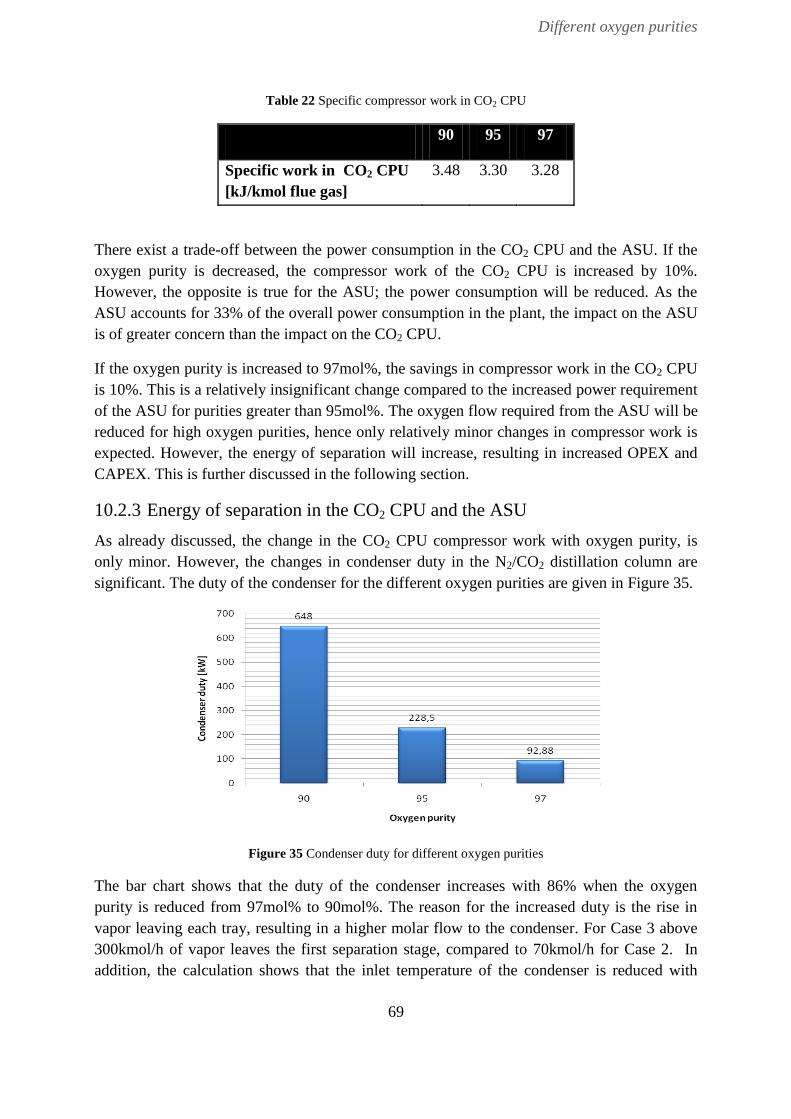
Different oxygen purities
69
Table 22 Specific compressor work in CO2 CPU
90 95 97
Specific work in CO2 CPU
[kJ/kmol flue gas]
3.48 3.30 3.28
There exist a trade-off between the power consumption in the CO2 CPU and the ASU. If the
oxygen purity is decreased, the compressor work of the CO2 CPU is increased by 10%.
However, the opposite is true for the ASU; the power consumption will be reduced. As the
ASU accounts for 33% of the overall power consumption in the plant, the impact on the ASU
is of greater concern than the impact on the CO2 CPU.
If the oxygen purity is increased to 97mol%, the savings in compressor work in the CO2 CPU
is 10%. This is a relatively insignificant change compared to the increased power requirement
of the ASU for purities greater than 95mol%. The oxygen flow required from the ASU will be
reduced for high oxygen purities, hence only relatively minor changes in compressor work is
expected. However, the energy of separation will increase, resulting in increased OPEX and
CAPEX. This is further discussed in the following section.
10.2.3 Energy of separation in the CO2 CPU and the ASU
As already discussed, the change in the CO2 CPU compressor work with oxygen purity, is
only minor. However, the changes in condenser duty in the N2/CO2 distillation column are
significant. The duty of the condenser for the different oxygen purities are given in Figure 35.
Figure 35 Condenser duty for different oxygen purities
The bar chart shows that the duty of the condenser increases with 86% when the oxygen
purity is reduced from 97mol% to 90mol%. The reason for the increased duty is the rise in
vapor leaving each tray, resulting in a higher molar flow to the condenser. For Case 3 above
300kmol/h of vapor leaves the first separation stage, compared to 70kmol/h for Case 2. In
addition, the calculation shows that the inlet temperature of the condenser is reduced with

Different oxygen purities
70
decreasing oxygen purity. The results from Hysys show that the temperature is -95⁰C for the
case 3, compared to -80⁰C for case 2.
Though the condenser duty of the CO2/N2 distillation is reduced with increasing oxygen
purity, the duty is below 1MW for all the different cases. The savings in condenser duty is
therefore considered insignificant compared to the changes in the ASU. The energy of
separation in the ASU will increase sufficiently if the purity is increased above 95mol%. The
separation will change from oxygen-nitrogen to oxygen-argon, which requires more energy,
and implementation of a supplementary distillation column. If the oxygen purity is reduced
there will be some savings in the ASU. However reducing the oxygen purity will increase the
size of the operation equipment. For AKSO’s concept the equipment size of the ASU is of
great concern, as the system is planned to be located off-shore.

Possibilities of integrating the ASU
71
11 Possibilities of integrating the ASU
As already mentioned the ASU accounts for a significant amount of the overall power
consumption in the base case. If the ASU is integrated with the power plant the overall power
consumption of the unit will be reduced. In this chapter the possibilities of integrating the
ASU will be discussed.
11.1 Methodology
Integrating the ASU could decrease the external utility requirements in the plant. If the
composite curve is shifted to the right, cold energy from the LNG could be utilized in the
ASU. The CC shifted to the right is shown in Figure 36.
Figure 36 Shifted CC
The unbroken red line indicates the original hot CC, while the dotted line indicates the shifted
CC. When shifting the curve to the right the temperature approach get closer. The system is
no longer a threshold system; hence shifting the curves will reduce the utility consumption.
To evaluate the possibility of integrating the ASU two simulation models are created. In the
first model, the ASU is integrated with the regasification train. Data used are collected from
the main simulation model (Case 1). The second model represents a conventional ASU. This
model is created to gain a standard of reference. The following simplifications apply:
- Only the equipment upstream the cold box are simulated (for both models), hence the
impact on the cold box will not be discussed.
- To simplify the problem the air compressors are assumed to be the only power
consuming unit in the ASU.
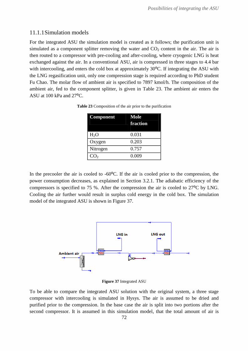
Possibilities of integrating the ASU
72
11.1.1 Simulation models
For the integrated ASU the simulation model is created as it follows; the purification unit is
simulated as a component splitter removing the water and CO2 content in the air. The air is
then routed to a compressor with pre-cooling and after-cooling, where cryogenic LNG is heat
exchanged against the air. In a conventional ASU, air is compressed in three stages to 4.4 bar
with intercooling, and enters the cold box at approximately 30⁰C. If integrating the ASU with
the LNG regasification unit, only one compression stage is required according to PhD student
Fu Chao. The molar flow of ambient air is specified to 7897 kmol/h. The composition of the
ambient air, fed to the component splitter, is given in Table 23. The ambient air enters the
ASU at 100 kPa and 27⁰C.
Table 23 Composition of the air prior to the purification
Component Mole
fraction
H2O 0.031
Oxygen 0.203
Nitrogen 0.757
CO2 0.009
In the precooler the air is cooled to -60⁰C. If the air is cooled prior to the compression, the
power consumption decreases, as explained in Section 3.2.1. The adiabatic efficiency of the
compressors is specified to 75 %. After the compression the air is cooled to 27⁰C by LNG.
Cooling the air further would result in surplus cold energy in the cold box. The simulation
model of the integrated ASU is shown in Figure 37.
Figure 37 Integrated ASU
To be able to compare the integrated ASU solution with the original system, a three stage
compressor with intercooling is simulated in Hysys. The air is assumed to be dried and
purified prior to the compression. In the base case the air is split into two portions after the
second compressor. It is assumed in this simulation model, that the total amount of air is

Possibilities of integrating the ASU
73
compressed in a three stage compressor. The simulation model of the conventional ASU is
given in Figure 38.
Figure 38 Conventional ASU
11.2 Results and discussion
The component splitter separates out the water and CO2 content in the ambient air, the
overhead molar flow is calculated to 7581kmol/h. In the first LNG heater the air is cooled to
-60⁰C by heating LNG to -152.1⁰C, as can be seen in Table 24. The air is than compressed in
a one-stage compressor. The outlet temperature of the compressor is calculated to 134.1 ⁰C.
Table 24 Properties of HXs prior and after the air compressor
Unit Th,inlet
[⁰C]
Th,outlet
[⁰C]
Tc,inlet
[⁰C]
Tc,outlet
[⁰C]
Duty
[MW]
Pre-cooler 27 -60 -160.3 -152.1 5.30
After-cooler 134.1 27 -152.1 -144,4 5.90
SUM 11.2
Table 24 shows that the overall duty of the HXs is calculated to 11.2 MW. This means that
11.2 MW of cold energy from the LNG regasification train is utilized in the ASU; hence the
utility consumption in the power plant can be reduced by the same amount. The compressor
work of the air compressor was calculated to 11.38 MW. The result from the simulation
model of the original system, gives a compressor duty of 13.3 MW. Thus, integrating the
ASU will result in 1.92 MW saving in compression work.
In Figure 39 the CC of the base case is shown to the left, while the CC when integrating the
ASU is shown to the right. As can be seen from the graphs the change in pinch point is
relatively small, and the temperature approach of the two graphs is only slightly reduced.
Hence, the increase in heat transfer area will not be significant if implementing this system
configuration.

Possibilities of integrating the ASU
74
Figure 39 Left: CC of base case. Right: CC when integrating the ASU.
The main issue if the ASU is heat integrated with the regasification train is regulation of the
ASU. From the simulation model it was found that if reducing the LNG load with 50%,
temperature cross will occur in the aftercooler. In addition, the outlet temperature of air will
be greater than 100⁰C. As the regulation of an ASU is found difficult, supplementary
heaters/coolers could be implemented to be able to run the unit during part load operations. If
the outlet temperature of LNG from the aftercooler is set, the case would be as stated above.
Hence, a supplementary air cooler is required. If instead the temperature of air is set, the
outlet temperature of LNG would decrease to -129⁰C. Hence, the utility requirements would
increase. A supplementary heater could be installed, and more LP steam produced when
required.

Proposed system
75
12 Proposed system
A proposed solution with heat integration between the CO2 CPU, the ASU, the regasification
train and the steam and power unit will be presented in this chapter. In addition, the
possibility of using membranes for air separation in AKSO’s system is discussed.
12.1 Chosen parameters and assumptions
12.1.1 Selected oxygen purity
As discussed in Chapter 10, decreasing the oxygen purity will decrease the required energy of
separation in the ASU. However, the investments cost is likely to increase, as the size of the
ASU will increase. If the oxygen purity is increased to 97mol%, the power consumption of
the CO2 CPU will decrease, but both capital and operational costs of the ASU will increase
sufficiently. As this is the main energy consuming unit in the facility, it is likely that
increasing the oxygen purity would be unprofitable. The selected oxygen purity is therefore
set to 95mol% in the proposed system configuration.
12.1.2 Selected heat integration scheme
As stated in Chapter 9 the sequence of the pair-matching is found acceptable. It is chosen to
heat integrate the ASU as the integration leads to lower power demand in the unit. The
integration scheme given in Chapter 11 will be implemented.
12.2 Proposed system configuration
The integration between the ASU and the regasification train can be seen in Figure 40. If the
LNG should be directly heat integrated with the ambient air, this will require pipes with a
significant diameter due to the high density of LNG. Therefore it could be profitable to use
indirect heating to reduce the investment cost. This is not further evaluated in this thesis.
Figure 40 Integration of the ASU
For the new system configuration the CC is shifted to the right, thus LNG heaters 1-5 are
shifted to a higher temperature. The streams follows logical from temperature as can be seen

Proposed system
76
in Figure 42, where the dotted line indicates the ASU. The steam generation will not be
affected by the integration of the ASU.
Figure 41 T-Q Diagram system with integrated ASU
The gains of implementing the proposed solution are as follows (compared to case 1):
1. The LP consumption is reduced to 3684 kmol/h
2. The duty of LNG heater 5 is reduced to 48.5 MW
3. No supercooling is experienced in LNG heater 4, as can be seen in Figure 42. Thus,
there is less risk of freeze-out in the system. In addition a greater temperature
approach between the steam condensate and the LNG is detected. This results in
decreased heat transfer area.
4. The power production in the LP turbine is increased to 14.41 MW.
5. The LNG will be shifted closer to the HTFs employed in LNG HX 1-3. This will lead
to greater driving forces in these HXs.
The disadvantages of implementing the new system configuration are:
1. The system configuration is more complex as the ASU is integrated with the power
and steam plant. A greater regulation system is required, and oxygen buffer tanks will
be necessary.
2. The ∆T in the different HXs will be reduced, which will affect the required heat
transfer area.

Proposed system
77
3. The capital expenses of the system might increase, due to the heat exchange between
the LNG train and the ASU.
12.3 Possibility of using ITMs for oxygen production
If reducing the power consumption in the system further, implementation of membranes could
be an option. As stated in Chapter 6 ITMs have the greatest potential of large-scale production
of high purity oxygen. As the MIECs do not require an electric circuit, these membranes
would be the best solution for an off-shore facility. In the following a proposition of a system
configuration with membranes is given. As MIECs are capable of producing oxygen with
99% purity, this would lead to energy savings in the CO2 CPU. To evaluate the savings, the
main simulation model is simulated for 99mol% oxygen purity. The results are given in
Chapter 12.5.
12.4 Possible configuration of the system
As the oxygen flux through the membrane is proportional to ln(p1/p2), a vacuum condition is
required on the permeate side or the air can be compressed to a high pressure prior to the
membranes. Both solutions will cause supplementary compressor work in the system, thus the
best system configuration should be based on an economical analysis.
The ideal membrane structure is dependent on several factors, as discussed in Chapter 6. For
AKSO’s system a production rate greater than 1000 tons/day is required. The most promising
perovskite, of those given in Table 4 is Ba0.5Sr0.5Co0.8Fe0.2O3-δ, as this membrane has a
relatively high flux (compared to other perovskites) and thickness. These membranes are 1.8
mm thick, and the oxygen flux is approximately 1.563 ∙10-6
mol/s∙cm2. This means that one of
these membranes can produce 1.013∙10-6
kmol/h oxygen. I.e. more than 1∙109 membranes in
stacks are required to produce the amount of oxygen needed in AKSO’s system.
If employing membranes for air separation, a similar system configuration as that given in
Section 6.3.2 should be implemented. The air can be heated firstly by the nitrogen from the air
separation. Thereby a hot utility is required to heat the air to at least 800ºC. This could be
done by burning part of the send-out gas in a supplementary burner. However, this would lead
to increased CAPEX and emissions. Another solution could be to utilize the flue gas from the
oxy-burner to heat the air prior to the separation, though this would decrease the steam
production in the HRSG.
If the technology develops as suggested by Ted Foster, implementing membranes for air
separation in AKSO’s system could be an economical option. As stated in Chapter 6 the cost
is intended to be 30 % lower than for an ASU configuration. In addition all ITMs produce
oxygen with greater than 99mol% purity, hence the implementation of membranes would
decrease the power consumption in the CO2 CPU. This will be discussed in the next section.

Proposed system
78
12.5 Impact on the CO2 CPU
To evaluate the savings, the main simulation model was tested for 99mol% oxygen purity.
The O2/N2 molar flow was specified to 1478 kmol/h. The recycle rate is held constant at 6250
kmol/h. The CO2 capture rate was adjusted to 0.9999. The results are given in the Table 25:
Table 25 Impact on the CO2 CPU
Parameter Unit Value
CO2 fraction in flue gas [mol%] 0.78
CO2 fraction flue gas to CO2CPU [mol%] 0.94
Molar flow to CO2 CPU [kmol/h] 790
Compressor work CO2 CPU kW 2500
Condenser duty kW 16
The condenser work of the N2/CO2 is significantly decreased when the oxygen purity is
increased to 99 mol%. In addition the molar flow of CO2 to the purification unit is decreased;
hence the CAPEX and OPEX of the unit are decreased, due to the reduction in equipment
size. The savings in the CO2 CPU are dependent on the selected utility used to heat air. If a
combustor is used, the flue gas from the burner should be purified. This would increase the
molar flow to the CO2 CPU, and decrease the CO2 fraction.
If implementation of membranes does not lead to increased CO2 production, the CO2 CPU
scheme could be changed to reduce both energy cost and CAPEX. As the CO2 fraction in the
flue gas to the CO2 CPU is nearly 95mol%, the no purification scheme could be a more
economical solution. In this scheme no distillation column is required. This will result in
lower investment and operation costs.

Conclusion and further work
79
13 Conclusion and further work
13.1 Conclusion
Simulation models were created in Aspen Hysys to investigate the heat integration in the
system, validate the feasibility of integrating an ASU and to find the impact on the CO2 CPU
when changing the oxygen purity.
The heat integration in AKSO’s system was found acceptable. The sequence of the pair-
matching of the streams was logical from temperature. However, it could be beneficial to
change the HTF in LNG heaters 2-3 to a HTF with a lower freezing point (e.g. Methanol).
The system was tested for three different oxygen purities; 90, 95 and 97mol%, where
95mol% is the oxygen purity employed in the base case. If reducing the purity the compressor
work of the CO2 CPU is increased by 10%, while the opposite is true if the purity is increased
to 97mol%. The duty of the condenser in the N2/CO2 distillation column is increased by 65%
if the purity is reduced to 90mol%. A literature review states that the energy of separation on
the ASU will increase sufficiently for purities above 95mol%. If the oxygen purity is reduced
however, only a minor reduction in separation energy is experienced. In addition, the
equipment size of the ASU will increase for purities below 95mol%. Base on the previous,
and owing to the fact that the ASU accounts for 33% of the overall power consumption in the
plant, the oxygen purity should not be changed.
Integrating the ASU with the power plant was found to be technically possible at full load.
However, it may be technical issues regarding regulation of the ASU when running the plant
at part load. If integrating the ASU the power consumption in the air compressors are reduced
with 14%. In addition, 18 % reduction in LP steam consumption is experienced. This results
in a greater turbine yield; approximately 2 MW increased power production. As the
equipment size, the OPEX and the energy cost the ASU is decreased if integrated with the
power plant, this is considered an adequate solution if it is found possible to regulate the unit
during part load operation.
If using membranes for air separation, MIECs with a perovskite structure should be
employed. The most promising structure found was Ba0.5Sr0.5Co0.8Fe0.2O3-δ. Today 1∙109
such membranes are required to produce enough oxygen. Hence, the technology needs to be
further evolved before it is feasible.
13.2 Further work
Implementation of membrane technology should be simulated in a model where the ITM is
integrated with the oxy-fuel plant. Special care should be addressed to the heating of the air
prior to the ITM. In addition, an economical analysis of the implementation should be carried
out.

Conclusion and further work
80
An economical evaluation on employing Methanol instead of MEG/Water as the HTF, in
LNG heaters 2-3 should be investigated. In addition the thermodynamic benefits of
changing the HTF should be investigated.
A complete simulation model of the ASU should be created in Aspen Hysys, to find the
accurate changes in power demand when changing the oxygen purity.
A study on possibilities of regulating an integrated ASU should be carried out. This
includes finding the impact on the cold box when the feed load changes.
List of References
81
List of References
1. Buhre, B.J.P., et al., Oxy-fuel combustion technology for coal-fired power generation. Progress in Energy and Combustion Science, 2005. 31(4): p. 283-307.
2. Amann, J.M., M. Kanniche, and C. Bouallou, Natural gas combined cycle power plant modified into an O2/CO2 cycle for CO2 capture. Energy conversion and management, 2009. 50(3): p. 510-521.
3. Metz, B., IPCC special report on carbon dioxide capture and storage. 2005: Cambridge University Press.
4. EIA. International Energy Outlook 2010. 2010; Available from: http://www.eia.doe.gov/oiaf/ieo/nat_gas.html.
5. Mario Ditaranto, Øyvind Langørgen, and L. Aksetøy, Oxy-Fuel Burners for a Zero Emission LNG Regasification Plant. 2010.
6. Yang, C. and Z. Huang, Lower emission LNG vaporization. LNG journal, 2004: p. 24. 7. Yang, C.C. Possible LNG Receving Terminal Air Emission sources and MItigation Procedures. in
Zeus LNG Conferance. 2006. Houston: Foster Wheeler. 8. AkerSolution, Zero Emission Power Production for LNG Regasification. 2010 9. Ministry of Petroleum and Energy. Carbon dioxide capture and storage. 2010; Available
from: http://www.regjeringen.no/en/dep/oed/Subject/carbon-capture-and-storage/capture-transport-and-storage-of-co2.html?id=443518.
10. Bolland, O., Power generation: CO2 Capture and Storage. 2010. 11. Krammer, G., Introduction to Combustion - Formation and Depletion of Air Pollutants. 2008. 12. McCauley, K., et al., Commercialization of oxy-coal combustion: Applying results of a large
30MWth pilot project. Energy Procedia, 2009. 1(1): p. 439-446. 13. Metz, B., Capture of CO2, in IPCC special report on carbon dioxide capture and storage. 2005,
Cambridge University Press. 14. European Technology Platform for Zero Emission Fossil Fuel Power Plants 2007. 15. Michael J. Moran and H.N. Shapiro, Fundamentals of Engineering Thermodynamics. Fifth ed.
2006: John Wiley & Sons. 16. Øverlie, J.M., Strømningsmaskiner, Bind 3. 1992: Tapir. 17. Romeo, L.M., et al., Optimization of intercooling compression in CO2 capture systems.
Applied Thermal Engineering, 2009. 29(8-9): p. 1744-1751. 18. Arora, R.C., Refrigeration and Air Conditioning. 2010: PHI. 19. Darde, A., et al., Air separation and flue gas compression and purification units for oxy-coal
combustion systems. Energy Procedia, 2009. 1(1): p. 527-534. 20. ya Nsakala, N., et al., Oxygen-fired circulating fluidized bed boilers for greenhouse gas
emissions control and other applications. 2004. 21. Wall, T.F., Combustion processes for carbon capture. Proceedings of the Combustion
Institute, 2007. 31(1): p. 31-47. 22. Bensakhria, A. and M. Leturia, Natural gas oxy-combustion with flue gas recycling for CO2
capture. CHEMICAL ENGINEERING, 2010. 21: p. 637-642. 23. Ochs, T., et al., Results of initial operation of the Jupiter Oxygen Corporation oxy-fuel 15
MWth burner test facility. Energy Procedia, 2009. 1(1): p. 511-518. 24. Smith, R., Choice of Separator for Hetregeneous Mixtures, in Chemical Process Design and
Integration. 2005, John Wiley and Son. 25. Kister, H.Z. and Knovel, Distillation design. 1992: McGraw-Hill New York. 26. Nakaiwa, M., et al., Evaluation of an energy supply system with air separation. Energy
conversion and management, 1996. 37(3): p. 295-301.

List of References
82
27. Smith, A. and J. Klosek, A review of air separation technologies and their integration with energy conversion processes. Fuel Processing Technology, 2001. 70(2): p. 115-134.
28. Richard Dubettier, et al., Air Separation Unit: Flexibility & Energy Storage, in 2nd Oxyfuel Combustion Conference, Air Liquide Engineering: France.
29. Nicklas Simonsson, Marie Anheden, and R. Dubettier, Develoment Opportunities for Future Large Scale Lignite Oxyfuel Power Plants, in 2nd Oxyfuel Combustion Conference: France.
30. Wilkinson, M.B., et al. CO2 capture via oxyfuel firing: optimisation of a retrofit design concept for a refinery power station boiler. 2001: Citeseer.
31. Hägg, M.-B., Handbook of Membrane Separations: Chemical, Pharmaceutical and Biotechnological Applications. 2006: NTNU.
32. Lichtenthaler, R.N. Forschung. Available from: http://www.uni-heidelberg.de/institute/fak12/PC/lichtenthaler/Forschung-RNL.html.
33. Burggraaf, A. and L. Cot, Fundamentals of inorganic membrane science and technology. 1996: Elsevier Science Ltd.
34. Bouwmeester HJM, B.A., Dense ceramic membranes for oxygen separation, in Fundamentals of Inorganic Membrane Science and technology 1996.
35. Dyer, P., et al., Ion transport membrane technology for oxygen separation and syngas production. Solid State Ionics, 2000. 134(1-2): p. 21-33.
36. Bose, A. and E. Corporation, Inorganic membranes for energy and fuel applications. 2007: Springer New York.
37. Geankoplis, C.J., Transport processes and separation process principles (includes unit operations). Fourth ed. 2003: Prentice Hall Press Upper Saddle River, NJ, USA.
38. Sunarso, J., et al., Mixed ionic-electronic conducting (MIEC) ceramic-based membranes for oxygen separation. Journal of Membrane Science, 2008. 320(1-2): p. 13-41.
39. Hashim, S., A. Mohamed, and S. Bhatia, Current status of ceramic-based membranes for oxygen separation from air. Advances in Colloid and Interface Science, 2010.
40. Li, K., Ceramic Membranes for Separation and Reaction 2007: John Wiley & Sons. 41. Sammells, A. and M. Mundschau, Nonporous inorganic membranes: for chemical processing.
2006: Vch Verlagsgesellschaft Mbh. 42. Shao, Z., et al., Investigation of the permeation behavior and stability of a Ba0. 5Sr0. 5Co0.
8Fe0. 2O3-[delta] oxygen membrane. Journal of Membrane Science, 2000. 172(1-2): p. 177-188.
43. Teraoka, Y., T. Nobunaga, and N. Yamazoe, Effect of cation substitution on the oxygen semipermeability of perovskite-type oxides. Chemistry Letters, 1988. 17(3): p. 503-506.
44. Wang, H., et al., A cobalt-free oxygen-permeable membrane based on the perovskite-type oxide Ba 0.5 Sr 0.5 Zn 0.2 Fe 0.8 O 3. Adv. Mater, 2005. 17(14): p. 1785–8.
45. Ted Foster, et al., Enabling Clean Energy Production from Coal: ITM Oxygen Development Update, in International Pittsburgh Coal Conference. 2009, Air products and Chemicals.
46. Ciferno, J., Pulverized Coal Oxycombustion Power Plants. Final Report, August, 2007. 47. Zhang, N. and N. Lior, Proposal and Analysis of a Novel Zero CO Emission Cycle With Liquid
Natural Gas Cryogenic Exergy Utilization. Journal of Engineering for Gas Turbines and Power, 2006. 128: p. 81.
48. Kemp, I.C., Pinch analysis and process integration: a user guide on process integration for the efficient use of energy. 2007: Butterworth-Heinemann.
49. Process Design Center. Energy pinch technology. 2009 [cited 2010 01.12]; Available from: http://www2.lse.ac.uk/library/services/training/endnote/Quick%20Tip%20citing%20webpages.aspx.
50. Al-Sobhi, S., H. Alfadala, and M. El-Halwagi. Simulation and Energy Integration of a Liquefied Natural Gas (LNG) Plant. 2009.
51. Smith, R., A quick one, T. Gundersen, Editor. 2011.
List of References
83
52. GETINER ENGINEERING CORPORATION. Physical Properties of Methanol: CH3OH. Available from: http://www.cetinerengineering.com/Properties.htm.
53. Frank P. Incropera, D.P.D., Theodore L. Bergman, Adrienne S. Lavine, Fundamentals of heat and mass transfer. sixth ed. 2007: John Wiley & Sons.
54. Kemp, I.C., Pinch Analysis and Process Integration. second edition ed. 2007: Elsevier Ltd. . 55. Bell, K.J., Introduction to heat exchanger design, in Heat exhanger design handbook. 1983,
Hemisphere Publishing Corporation. 56. Rev, E. and Z. Fonyo, Diverse pinch concept for heat exchange network synthesis: the case of
different heat transfer conditions. Chemical engineering science, 1991. 46(7): p. 1623-1634. 57. Hamid, A. and M. Kamaruddin, HYSYS: an introduction to chemical engineering simulation for
UTM Degree++ program. 2007. 58. Aspen Tech, HYSYS 2004.2 Operations Guide. 2005.

Appendices
84

Appendices
85
Appendices
Appendix A: Simulation model
Appendix B: Interpolation in steam tables
Appendix C: Input/output data from PRO-PI
Appendix D: Results – different oxygen purities
Appendix E: Mail from Ted Foster, Air Products

Appendices
86

Appendices
i
Appendix A
A.1 Simulation model
Figure A.1 shows the main simulation model created in Aspen Hysys. The properties of
LNG/NG are found in Table A.1. The properties of the steam cycle are found in Table A.2.
The properties of the flue gas are found in Table A.3. The duty of the heater/coolers is given
in Table A.4. Table A.5 gives the power consumption/production in the different units.
Table A.1 Stream data LNG train
Stream Nr F1 F2 F3 F4 F5 F6 F7 F8 F9
Temperature -160,3 -154,6 -151,4 -114,14 -56,82 3,9 3,9 -44,37 26,96
Pressure 80 79,7 79,4 79,1 78,8 78,5 78,5 2,5 2
Molar flow 4,48∙104
4,48∙104 4,48∙10
4 4,48∙10
4 4,48∙10
4 4,48∙10
4 693 693 693
Mol% (CH4) 0,925 0,925 0,925 0,925 0,925 0,925 0,925 0,925 0,925
Mol% (C2H6) 0,055 0,055 0,055 0,055 0,055 0,055 0,055 0,055 0,055
Mol%(C3H8) 0,01 0,01 0,01 0,01 0,01 0,01 0,01 0,01 0,01
Mol% (N2) 0,01 0,01 0,01 0,01 0,01 0,01 0,01 0,01 0,01
Table A.2 Stream data steam cycle
Stream Nr S1 S2 S3 S4 S5 S6 S7 S8 S9
Temperature 25 25,53 155 251,9 398,3 176,5 176,5 176,5 16,29
Pressure 1,5 54,70 54,50 41,07 40,91 5,0 5,0 5,0 4,7
Molar flow 1,02∙104
1,02∙104 1,02∙10
4 9956 9956 9956 4506 4361 4361
Mol% (H2O) 1 1 1 1 1 1 1 1 1
Stream Nr S10 S11 S12 S13 S14
Temperature 176,5 11,42 176,5 52,58 5,7
Pressure 5,0 4,7 5,0 0,14 0,13
Molar flow 145 145 5450 5450 5450
Mol% (H2O) 1 1 1 1 1
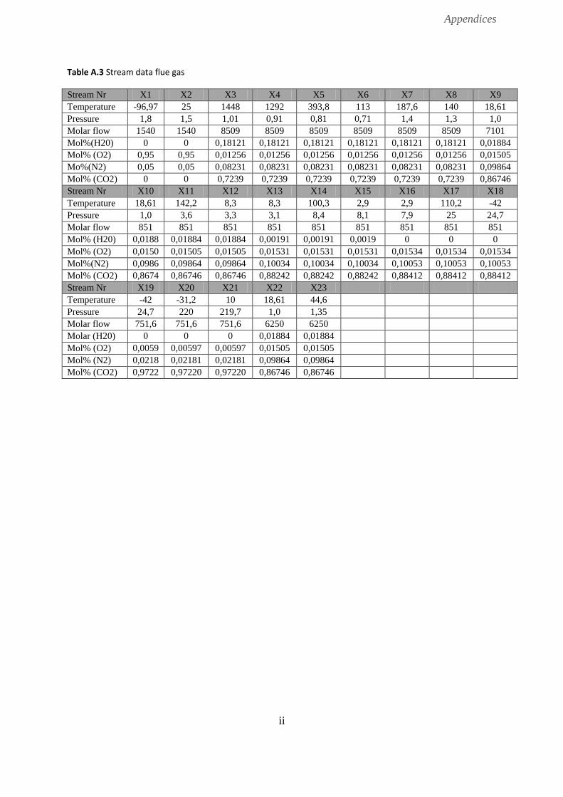
Appendices
ii
Table A.3 Stream data flue gas
Stream Nr X1 X2 X3 X4 X5 X6 X7 X8 X9
Temperature -96,97 25 1448 1292 393,8 113 187,6 140 18,61
Pressure 1,8 1,5 1,01 0,91 0,81 0,71 1,4 1,3 1,0
Molar flow 1540 1540 8509 8509 8509 8509 8509 8509 7101
Mol%(H20) 0 0 0,18121 0,18121 0,18121 0,18121 0,18121 0,18121 0,01884
Mol% (O2) 0,95 0,95 0,01256 0,01256 0,01256 0,01256 0,01256 0,01256 0,01505
Mo%(N2) 0,05 0,05 0,08231 0,08231 0,08231 0,08231 0,08231 0,08231 0,09864
Mol% (CO2) 0 0 0,7239 0,7239 0,7239 0,7239 0,7239 0,7239 0,86746
Stream Nr X10 X11 X12 X13 X14 X15 X16 X17 X18
Temperature 18,61 142,2 8,3 8,3 100,3 2,9 2,9 110,2 -42
Pressure 1,0 3,6 3,3 3,1 8,4 8,1 7,9 25 24,7
Molar flow 851 851 851 851 851 851 851 851 851
Mol% (H20) 0,0188 0,01884 0,01884 0,00191 0,00191 0,0019 0 0 0
Mol% (O2) 0,0150 0,01505 0,01505 0,01531 0,01531 0,01531 0,01534 0,01534 0,01534
Mol%(N2) 0,0986 0,09864 0,09864 0,10034 0,10034 0,10034 0,10053 0,10053 0,10053
Mol% (CO2) 0,8674 0,86746 0,86746 0,88242 0,88242 0,88242 0,88412 0,88412 0,88412
Stream Nr X19 X20 X21 X22 X23
Temperature -42 -31,2 10 18,61 44,6
Pressure 24,7 220 219,7 1,0 1,35
Molar flow 751,6 751,6 751,6 6250 6250
Molar (H20) 0 0 0 0,01884 0,01884
Mol% (O2) 0,0059 0,00597 0,00597 0,01505 0,01505
Mol% (N2) 0,0218 0,02181 0,02181 0,09864 0,09864
Mol% (CO2) 0,9722 0,97220 0,97220 0,86746 0,86746

Appendices
iii

Appendices
iv
Table A.4 Duty of heater/coolers
Unit LNG HX1 LNG HX2 LNG HX3 LNG HX4 LNG HX5
Duty[MW] 4,1 2,3 28,2 63,3 59,7
Unit BFW heater Boiler Boiler_2 Superheater O2 /fuel preheater
Duty[MW] 27,7 107,2 107,2 20,4 2
Unit LNG heater1 LNG heater 2 LNG heater 3 LNG heater 4 LNG heater 5
Duty[MW] 1,4 0,9 4,1 63,3 59,7
Unit Oxygen preheater Fuel gas preheater Flue gas cond. Condenser
Duty[MW] 1,5 0,5 28,2 0,228
Table A.5 Power production/consumption
Unit LNG
pumps
BFW pump CO2 pump LP turbine MP turbine Flue gas fan Comp.
Duty [MW] 5,0 0,36 0,2 12,52 20,26 6,95
Unit C1 C2 C3 Air Fan Recycle comp Flue gas fan cooler
Duty[MW] 1,12 0,8 0,9 0,75 1,67 4,5
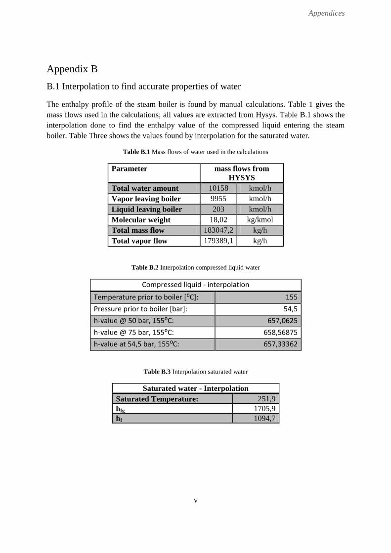
Appendices
v
Appendix B
B.1 Interpolation to find accurate properties of water
The enthalpy profile of the steam boiler is found by manual calculations. Table 1 gives the
mass flows used in the calculations; all values are extracted from Hysys. Table B.1 shows the
interpolation done to find the enthalpy value of the compressed liquid entering the steam
boiler. Table Three shows the values found by interpolation for the saturated water.
Table B.1 Mass flows of water used in the calculations
Parameter mass flows from
HYSYS
Total water amount 10158 kmol/h
Vapor leaving boiler 9955 kmol/h
Liquid leaving boiler 203 kmol/h
Molecular weight 18,02 kg/kmol
Total mass flow 183047,2 kg/h
Total vapor flow 179389,1 kg/h
Table B.2 Interpolation compressed liquid water
Compressed liquid - interpolation
Temperature prior to boiler [⁰C]: 155
Pressure prior to boiler [bar]: 54,5
h-value @ 50 bar, 155⁰C: 657,0625
h-value @ 75 bar, 155⁰C: 658,56875
h-value at 54,5 bar, 155⁰C: 657,33362
Table B.3 Interpolation saturated water
Saturated water - Interpolation
Saturated Temperature: 251,9
hfg 1705,9
hf 1094,7

Appendices
vi
Appendix C
C: Input data to PRO PI
PRO-PI draws the CC and GCC based on temperatures and duties of the different streams.
The input data is given in Table C.1
Table C.1 Input data to PRO PI
T start
[⁰C]
T target
[⁰C]
Duty
[MW]
Type
25,53 155 27,7 Cold 155 251,9 22,24 Cold
251,90 252 85,01 Cold
252,00 398,1 20,42 Cold
-160,3 -114,1 34,6 Cold
-144,1 -102,63 9,544 Cold
-102,632 -91,18 10,32 Cold
-91,1795 -79,727 11,597 Cold
-79,7274 -68,275 13,88 Cold
-68,2753 -56,823 17,9 Cold
-56,8232 3,921 59,7 Cold
-44,37 26,96 0,5 Cold
-96,97 25 1,5 Cold
1448 113 155,35 Hot
145 18,62 28,2 Hot
141,6 7,7 1,4 Hot
106,8 -43,1 4,1 Hot
99,96 2,24 0,9 Hot
52,58 52,43 6,33 Hot
52,43 52,28 6,33 Hot
52,28 52,13 6,33 Hot
52,13 51,98 6,33 Hot
51,98 51,83 6,33 Hot
51,83 51,7 6,33 Hot
51,7 51,5 6,33 Hot
51,5 51,37 6,32 Hot
51,37 51,22 6,34 Hot
51,22 7,75 6,33 Hot
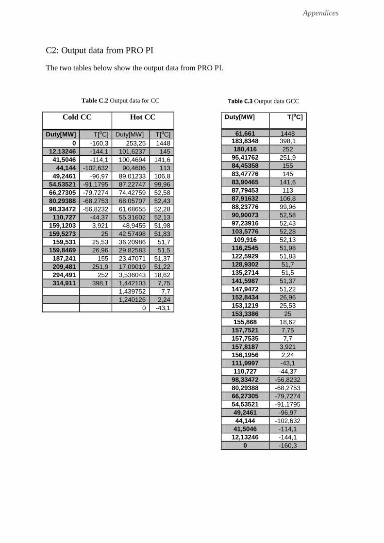
Appendices
vii
C2: Output data from PRO PI
The two tables below show the output data from PRO PI.
Table C.2 Output data for CC
Cold CC Hot CC
Duty[MW] T[⁰C] Duty[MW] T[⁰C]
0 -160,3 253,25 1448
12,13246 -144,1 101,6237 145
41,5046 -114,1 100,4694 141,6
44,144 -102,632 90,4606 113
49,2461 -96,97 89,01233 106,8
54,53521 -91,1795 87,22747 99,96
66,27305 -79,7274 74,42759 52,58
80,29388 -68,2753 68,05707 52,43
98,33472 -56,8232 61,68655 52,28
110,727 -44,37 55,31602 52,13
159,1203 3,921 48,9455 51,98
159,5273 25 42,57498 51,83
159,531 25,53 36,20986 51,7
159,8469 26,96 29,82583 51,5
187,241 155 23,47071 51,37
209,481 251,9 17,09019 51,22
294,491 252 3,536043 18,62
314,911 398,1 1,442103 7,75
1,439752 7,7
1,240126 2,24
0 -43,1
Table C.3 Output data GCC
Duty[MW] T[⁰C]
61,661 1448 183,8348 398,1
180,416 252
95,41762 251,9
84,45358 155
83,47776 145
83,90465 141,6
87,79453 113
87,91632 106,8
88,23776 99,96
90,90073 52,58
97,23916 52,43
103,5776 52,28
109,916 52,13
116,2545 51,98
122,5929 51,83
128,9302 51,7
135,2714 51,5
141,5987 51,37
147,9472 51,22
152,8434 26,96
153,1219 25,53
153,3386 25
155,868 18,62
157,7521 7,75
157,7535 7,7
157,8187 3,921
156,1956 2,24
111,9997 -43,1
110,727 -44,37
98,33472 -56,8232
80,29388 -68,2753
66,27305 -79,7274
54,53521 -91,1795
49,2461 -96,97
44,144 -102,632
41,5046 -114,1
12,13246 -144,1
0 -160,3
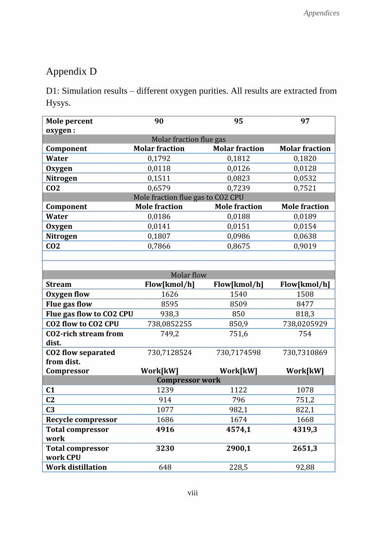
Appendices
viii
Appendix D
D1: Simulation results – different oxygen purities. All results are extracted from
Hysys.
Mole percent oxygen :
90 95 97
Molar fraction flue gas Component Molar fraction Molar fraction Molar fraction
Water 0,1792 0,1812 0,1820
Oxygen 0,0118 0,0126 0,0128
Nitrogen 0,1511 0,0823 0,0532
CO2 0,6579 0,7239 0,7521 Mole fraction flue gas to CO2 CPU
Component Mole fraction Mole fraction Mole fraction
Water 0,0186 0,0188 0,0189
Oxygen 0,0141 0,0151 0,0154
Nitrogen 0,1807 0,0986 0,0638
CO2 0,7866 0,8675 0,9019
Molar flow
Stream Flow[kmol/h] Flow[kmol/h] Flow[kmol/h]
Oxygen flow 1626 1540 1508
Flue gas flow 8595 8509 8477
Flue gas flow to CO2 CPU 938,3 850 818,3
CO2 flow to CO2 CPU 738,0852255 850,9 738,0205929
CO2-rich stream from dist.
749,2 751,6 754
CO2 flow separated from dist.
730,7128524 730,7174598 730,7310869
Compressor Work[kW] Work[kW] Work[kW] Compressor work
C1 1239 1122 1078
C2 914 796 751,2
C3 1077 982,1 822,1
Recycle compressor 1686 1674 1668
Total compressor work
4916 4574,1 4319,3
Total compressor work CPU
3230 2900,1 2651,3
Work distillation 648 228,5 92,88
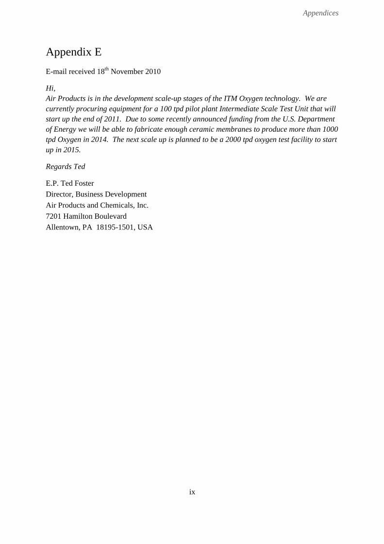
Appendices
ix
Appendix E
E-mail received 18th
November 2010
Hi,
Air Products is in the development scale-up stages of the ITM Oxygen technology. We are
currently procuring equipment for a 100 tpd pilot plant Intermediate Scale Test Unit that will
start up the end of 2011. Due to some recently announced funding from the U.S. Department
of Energy we will be able to fabricate enough ceramic membranes to produce more than 1000
tpd Oxygen in 2014. The next scale up is planned to be a 2000 tpd oxygen test facility to start
up in 2015.
Regards Ted
E.P. Ted Foster
Director, Business Development
Air Products and Chemicals, Inc.
7201 Hamilton Boulevard
Allentown, PA 18195-1501, USA