energy harvesting and control of a regenerative suspension ... · dr. krishna vijayaraghavan,...
TRANSCRIPT
Energy Harvesting and Control of a Regenerative
Suspension System using Switched Mode Converters
by
Chen-Yu Hsieh
M.ASc. (Electrical and Computer Engineering), Concordia University, 2011
B.Sc. (Electrical and Computer Engineering), University of Ottawa, 2008
Thesis Submitted in Partial Fulfillment of the
Requirements for the Degree of
Doctor of Philosophy
in the
School of Mechatronic Systems Engineering
Faculty of Applied Sciences
Chen-Yu Hsieh 2014
SIMON FRASER UNIVERSITY
Fall 2014

ii
Approval
Name: Chen-Yu Hsieh
Degree: Doctor of Philosophy
Title: Energy Harvesting and Control of a Regenerative Suspension
System using Switched Mode Converters
Examining Committee: Chair: Dr. Carolyn Sperry, P.Eng.
Assistant Profesor, School of Mechatronic Systems
Engineering
Dr. Farid Golnaraghi, P.Eng.
Co-Senior Supervisor
Professor
Dr. Mehrdad Moallem, P.Eng.
Co-Senior Supervisor
Professor
Dr. Jiacheng Wang, P.Eng.
Supervisor
Assistant Professor
Dr. Krishna Vijayaraghavan, P.Eng.
Internal Examiner
Assistant Professor
School of Mechatronic Systems
Engineering
Dr. Shahruar Mirab, P.Eng.
External Examiner
Professor
Electrical and Computer Engineering,
University of British Columbia
Date Defended/Approved: December 12, 2014

iii
Partial Copyright License
iv
Abstract
Harvesting road induced vibration energy through electromagnetic suspension allows
extension of the travel range of hybrid and fully electrical powered vehicles while achieving
passenger comfort. The core of this work is to investigate development of power converters for an
electromagnetic suspension system which allows for regeneration of vibration energy and
dynamics control of vehicle suspension. We present a variable electrical damper mechanism
which can be controlled using unity power-factor AC/DC converter topologies. By controlling the
synthesized electrical damper, the system is capable of providing variable damping forces,
ranging from under-damped to over-damped cases, while regenerating mechanical vibration
energy into electric charge stored in a battery. To demonstate the concept, the developed
converter is attached to a small-scale one-degree-of-freedom suspension prototype which
emulates a vehicle suspension mechanism. The energy regeneration mechanism consists of a
mass-spring system and a ball-screw motion converter mechanism coupled to a DC machine,
excited by a hydraulic shaker. The motion converter stage converts vibrational motion into a bi-
directional rotatory motion, resulting in generation of back-emf in the rotary machine. We also
introduce an optimized start/stop algorithm for the harvesting of energy using the proposed power
converter. The algorithm allows for improvements in power conversion efficiency enhancement
(≈ 14% under class C road profile) through turning the circuit on/off during its operation. The
idea is to ensure that the converter only operates in the positive conversion efficiency region;
meaning that when there is enough energy the converter starts the energy harvesting process.
Furthermore, an estimation of range enhancement for a full-scale electric vehicle (EV) is
furnished using regenerative suspension. It is estimated that for a full size EV (e.g., Tesla model
S), a range extension of 10-30% is highly realistic, depending on the road conditions.
Keywords: Energy harvesting, bi- directional switch- mode rectifier, direct AC/DC
converter, regenerative Sky-hook control, regenerative suspension system,
variable electrical damper.

v
Dedication
For my parents.

vi
Acknowledgements
I would like to take this opportunity to acknowledge the invaluable technical and
personal supervisions by Dr. Farid Golnaraghi, Dr. Mehrdad Moallem. With their strong technical
and financial supports allowed me to persevere through the years of my Ph.D study at Simon
Fraser University, BC. Moreover, I would like to thank my comitte members Dr. Jiacheng Wang
and Dr. Shahriar Mirabbasi from University of British Columbia for taking their time and effort
in reviewing my thesis. Lastly, I would like to thank my collegue Mr. Bo Huang for the greatful
research collaborations.
Mostly importantly, I would like to express deep gratitudes to my parents, relatives, and
Grace Chen for their strong support in making my Ph.D pursing days the most pleasant periods of
my academic journey.

vii
Table of Contents
Approval .......................................................................................................................................... ii
Partial Copyright License ............................................................................................................... iii
Abstract ........................................................................................................................................... iv
Dedication ........................................................................................................................................ v
Acknowledgements ......................................................................................................................... vi
Table of Contents .......................................................................................................................... vii
List of Tables .................................................................................................................................... x
List of Figures ................................................................................................................................. xi
List of Acronyms ......................................................................................................................... xvii
Nomenclature ............................................................................................................................. xviii
Chapter 1. Introduction ............................................................................................................ 1
1.1. Present State of Vehicular Suspension Control ...................................................................... 3
1.1.1. Delphi Automotive Magne-Ride .............................................................................. 4
1.1.2. Daimler- Benz AG Magic Body Control ................................................................. 5
1.2. Electromagnetic Vehicular Suspensions ................................................................................. 6
1.2.1. Linear permanent magnets (PM) Actuator ............................................................... 6
1.2.2. Rotational DC Machine ........................................................................................... 7
1.3. Root Mean Square Optimization for Improved Vehicle Performance ................................... 7
1.4. Chapter Summary ................................................................................................................... 9
Chapter 2. Energy Harvesting of Regenerative Vehicular Suspension and Road
Excitation Modeling ............................................................................................. 11
2.1. Regenerative Mechatronic System ....................................................................................... 11
2.1.1. Electro- Mechanical Analogy ................................................................................ 15
2.1.2. Analytical Analysis of Forced Oscillator with Nonlinear Stiffness ....................... 19
2.1.3. Electric Generator with Shunt Resistor .................................................................. 24
2.2. Regenerative Suspension Prototype Modeling ..................................................................... 27
2.2.1. Regenerative Suspension Prototype ....................................................................... 29
2.3. Regenerative Power Electronics Topologies ........................................................................ 32
2.4. Construction of Standardized Road Profiles ......................................................................... 34
2.5. Full- sized Vehicle Power Regeneration Potential ............................................................... 38
2.6. Chapter Summary ................................................................................................................. 41
Chapter 3. Bi- directional Switch Mode Rectifier for Synthesizing Variable
Damping and Semi- Active Control ................................................................... 42
3.1. Converter Modeling .............................................................................................................. 42
3.2. Regeneration and Motoring Modes ...................................................................................... 45
3.3. Hysteresis Current Control ................................................................................................... 47
3.3.1. Double- band Three-level Hysteresis Current Control .......................................... 47
Variable Resistor Synthesis using Three- level HCC ......................................................... 52
3.3.2. Multi- level Hysteresis Current Control................................................................. 54

viii
3.3.3. Proportional Integral/ State Space Feedback Control of Switch Mode
Rectifier for Variable Resistor Synthesis ............................................................... 60
Terminal Transfer Function ................................................................................................ 62
3.4. Switch Mode Rectifier Prototype ......................................................................................... 63
3.5. Experimental Variable Resistor Synthesis under Suspension Harmonic Excitations ........... 65
3.6. Vibrational Frequency Sweep with Fixed Excitation Amplitude and Synthesized
Resistance ............................................................................................................................. 67
3.6.1. Regeneration Mode ................................................................................................ 67
3.6.2. Motoring Mode ...................................................................................................... 68
3.6.3. Mechatronic System Conversion Efficiency .......................................................... 69
3.7. Experimental Variable Resistor Synthesis under ISO Standard Excitations ........................ 73
3.7.1. Average Harvested Power/ Energy ........................................................................ 76
3.8. Regenerative Semi-Active Control using SMR .................................................................... 78
3.8.1. Simulation Results ................................................................................................. 80
3.8.2. Experimental Skyhook Detection .......................................................................... 83
3.8.3. Instantaneous Regenerative Semi-active Control .................................................. 86
3.8.4. Experimental Frequency Response with Regenerative Automotive
Suspension ............................................................................................................. 88
3.9. Chapter Summary ................................................................................................................. 90
Chapter 4. Bridgeless AC/DC Converter for Synthesizing Variable Damping ................. 91
4.1. Comparison of Energy Harvesting Circuit Topologies ........................................................ 92
4.2. Proposed Bridgeless Converter Topology ............................................................................ 94
4.3. Converter Analysis and Modelling ....................................................................................... 96
4.3.1. Modes 1 and 3 ........................................................................................................ 96
4.3.2. Modes 2 and 4 ........................................................................................................ 98
4.3.3. Converter Synthesized Resistor ............................................................................. 98
4.4. Simulation Results with Single Tone AC Source ............................................................... 102
4.4.1. Line Voltage, Line Current, and Filtered Line Current ....................................... 102
4.4.2. Inductor and Rectifying Diode Current ............................................................... 103
4.4.3. Power Efficiency .................................................................................................. 105
4.5. Experimental Results with Single Tone AC Source ........................................................... 107
4.5.1. Current switching waveforms and Variable Resistor Synthesis .......................... 108
4.5.2. Variable Resistor Synthesis ................................................................................. 110
4.5.3. Load Capacitor Voltage ....................................................................................... 111
4.6. Variable Synthesized Resistor with Fixed Excitation Frequency ....................................... 113
4.7. Variable Excitation Frequency with Fixed Synthesized Resistor ....................................... 115
4.8. Average Harvested Power .................................................................................................. 117
4.9. Chapter Summary ............................................................................................................... 118
Chapter 5. Autonomous Start/ Stop Algorithm .................................................................. 119
5.1. Auxiliary Circuit ................................................................................................................. 123
5.2. Adaptive Algorithm with ISO-standard Drive Cycle ......................................................... 125
5.3. Efficiency Enhancement ..................................................................................................... 128
5.4. Chapter Summary ............................................................................................................... 129

ix
Chapter 6. Conclusions and Suggestions for Future Work ............................................... 131
6.1. Suggestions for Future Work .............................................................................................. 133
6.1.1. A Bandwidth Enhanced Regenerative Suspension System ................................. 133
6.1.2. Frequency Response and Jump phenomena ......................................................... 134
References….. ............................................................................................................................. 136

x
List of Tables
Table 2-1: Adopted electro- mechanical analogy ........................................................................... 17
Table 2-2: Equivalent mass, damping coefficient and excitation amplitude. ................................. 28
Table 2-3: Applied damping ratios to electromagnetic suspension prototype with respect
to various load resistors. ....................................................................................... 31
Table 2-4: Regenerative suspension experimental parameter values ............................................. 32
Table 3-1: Truth table of 5- level HCC switching combinations ................................................... 56
Table 3-2: Values of ontroller gains and passive elements ............................................................ 63
Table 3-3. Power components selected for switching waveform and power efficiency
simulation. ............................................................................................................ 64
Table 3-4: Average harvested power (mW) various Rin under class C and D roughness. .............. 77
Table 3-5: Total estimated energy harvested (in Watt- hour) with Rin = 10 and 50 Ω under
ISO class C and D roughness. .............................................................................. 78
Table 3-6 Normalized RMS of acceleration and relative displacement and average
harvested power obtained with different values of Rin ......................................... 89
Table 4-1: Energy harvesting topologies comparisons ................................................................... 93
Table 4-2: Power components selected for switching waveform and power efficiency
simulation. .......................................................................................................... 107
Table 5-1: Auxiliary circuit components and ICs ........................................................................ 124
Table 5-2: Composition of Driving Cycle Time. ......................................................................... 128
Table 5-3: Comparisons of conversion efficiency with start/ stop algorithm............................... 129

xi
List of Figures
Figure 1-1: Tesla Model S [4]. ......................................................................................................... 2
Figure 1-2: Tesla Model X [5].......................................................................................................... 2
Figure 1-3: ADVANCED AGILITY with PRE- SCAN suspension [12]. ....................................... 6
Figure 1-4: (a) Line of minima maxima for lowest RMS of absolute acceleration and (b)
line of maxima for highest RMS of absolute acceleration for a specified
suspension relative displacement. (c) Design chart and (d) state diagram
for choosing optimal ωn and ζ are delineated by RMS absolute
acceleration line of minima with respect to RMS relative displacements. ............. 9
Figure 2-1: A two degree-of-freedom base excitation model. ........................................................ 12
Figure 2-2: (a) Amplitude and (b) phase of tire mass- base dynamics and the (c)
corresponding instantaneous response with excitation frequency of 1 and
10 Hz. ................................................................................................................... 13
Figure 2-3: Rendition of SDOF Mercedes- Benz S class front suspension under road-
excitation [12]. ..................................................................................................... 15
Figure 2-4: SDOF base excitation model. ...................................................................................... 15
Figure 2-5: Equivalent RLC circuit of a base- excited mass- spring damper model. ..................... 16
Figure 2-6: Non-dimensionalized frequency response of (a) sprung mass absolute
acceleration (b) suspension relative displacement. .............................................. 18
Figure 2-7: Variation of a and γ (ao =1, γo=1) with T1 for σ=0.05, f=0.5, µ=0.1 ............................ 21
Figure 2-8: Analytical and numerical simulation of systems response (blue: numerical
results) .................................................................................................................. 23
Figure 2-9: Electric generator in parallel connection to resistive load. .......................................... 24
Figure 2-10: Equivalent circuit of electric generator in parallel connection to resistive
load. ...................................................................................................................... 25
Figure 2-11: Regenerative suspension 1-DOF dynamic model. ..................................................... 28
Figure 2-12: Electromagnetic suspension prototype test bed. ........................................................ 30
Figure 2-13: Experimental frequency response of (a) amplitude of relative displacements
and (b) absolute acceleration with respect to various physical load
resistors (Ω). Undamped natural frequency ≈ 6 Hz. ............................................. 31
Figure 2-14: Analogous electrical model of 1-DOF regenerative suspension. .............................. 33
Figure 2-15: (a) PSD Φ(Ω) and (b) road profile X (in cm) of ISO 8608 road class B to D............ 35
Figure 2-16: Nominal longitudinal class C road profiles with (a) i= 1, 2 and (b) 100, 200
within 100 samples. .............................................................................................. 36
Figure 2-17: (a) Instantaneous waveform and (b) spectra amplitude of a white noise with
unit intensity. Sampling frequency: 0.5 Mhz. ...................................................... 37
xii
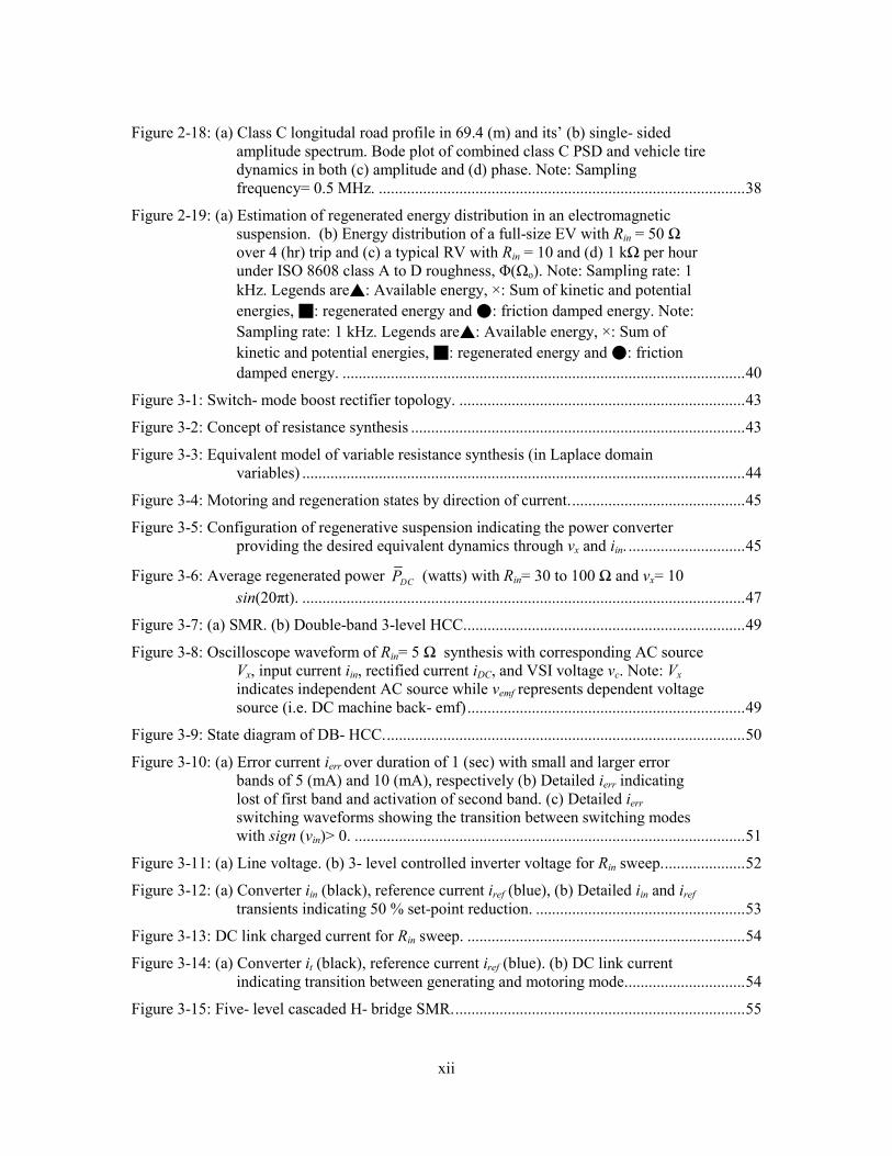
Figure 2-18: (a) Class C longitudal road profile in 69.4 (m) and its’ (b) single- sided
amplitude spectrum. Bode plot of combined class C PSD and vehicle tire
dynamics in both (c) amplitude and (d) phase. Note: Sampling
frequency= 0.5 MHz. ........................................................................................... 38
Figure 2-19: (a) Estimation of regenerated energy distribution in an electromagnetic
suspension. (b) Energy distribution of a full-size EV with Rin = 50 Ω
over 4 (hr) trip and (c) a typical RV with Rin = 10 and (d) 1 kΩ per hour
under ISO 8608 class A to D roughness, Φ(Ωo). Note: Sampling rate: 1
kHz. Legends are: Available energy, ×: Sum of kinetic and potential
energies, : regenerated energy and : friction damped energy. Note:
Sampling rate: 1 kHz. Legends are: Available energy, ×: Sum of
kinetic and potential energies, : regenerated energy and : friction
damped energy. .................................................................................................... 40
Figure 3-1: Switch- mode boost rectifier topology. ....................................................................... 43
Figure 3-2: Concept of resistance synthesis ................................................................................... 43
Figure 3-3: Equivalent model of variable resistance synthesis (in Laplace domain
variables) .............................................................................................................. 44
Figure 3-4: Motoring and regeneration states by direction of current. ........................................... 45
Figure 3-5: Configuration of regenerative suspension indicating the power converter
providing the desired equivalent dynamics through vx and iin. ............................. 45
Figure 3-6: Average regenerated power DCP (watts) with Rin= 30 to 100 Ω and vx= 10
sin(20πt). .............................................................................................................. 47
Figure 3-7: (a) SMR. (b) Double-band 3-level HCC. ..................................................................... 49
Figure 3-8: Oscilloscope waveform of Rin= 5 Ω synthesis with corresponding AC source
Vx, input current iin, rectified current iDC, and VSI voltage vc. Note: Vx
indicates independent AC source while vemf represents dependent voltage
source (i.e. DC machine back- emf) ..................................................................... 49
Figure 3-9: State diagram of DB- HCC. ......................................................................................... 50
Figure 3-10: (a) Error current ierr over duration of 1 (sec) with small and larger error
bands of 5 (mA) and 10 (mA), respectively (b) Detailed ierr indicating
lost of first band and activation of second band. (c) Detailed ierr
switching waveforms showing the transition between switching modes
with sign (vin)> 0. ................................................................................................. 51
Figure 3-11: (a) Line voltage. (b) 3- level controlled inverter voltage for Rin sweep. .................... 52
Figure 3-12: (a) Converter iin (black), reference current iref (blue), (b) Detailed iin and iref
transients indicating 50 % set-point reduction. .................................................... 53
Figure 3-13: DC link charged current for Rin sweep. ..................................................................... 54
Figure 3-14: (a) Converter it (black), reference current iref (blue). (b) DC link current
indicating transition between generating and motoring mode.............................. 54
Figure 3-15: Five- level cascaded H- bridge SMR. ........................................................................ 55

xiii
Figure 3-16: Five level HCC state diagram. The error- bands are defined by both ∆I and
∆Is. ........................................................................................................................ 56
Figure 3-17: (a) Line voltage, (b) converter current, (c) error current, and (d) inverter
generated voltage. vx= 15 sin(20πt) and vDC= 12 V. ............................................. 57
Figure 3-18: Detailed (a) line voltage, (b) converter current, (c) error current, and (d)
inverter generated voltage indicating transition of modes due to smaller
error-band lost of regulation. ................................................................................ 58
Figure 3-19: Detailed (a) line voltage, (b) converter current, (c) error current, and (d)
inverter generated voltage indicating controller reducing ierr for 50%
input change. ........................................................................................................ 58
Figure 3-20: (a) Line voltage, (b) converter current, rectified current of (c) first bridge,
and (d) second bridge indicating bi- directional power flow................................ 59
Figure 3-21: Simplified model of SMR (a) without and (b) with low pass filter driven by
ideal voltage source (i.e. Rint= 0 Ω). ..................................................................... 61
Figure 3-22: Desired synthesized resistor Rin= 10 Ω (green) and terminal transfer function
(red). ..................................................................................................................... 63
Figure 3-23: (a) PCB prototyped bi-directional bridgeless AC/DC converter. (b)
Regenerative automotive suspension prototype. (c) Test bed setup for
variable resistor synthesis. .................................................................................... 64
Figure 3-24: (a) Desired resistor synthesis sweep from Rin= 10 to 100 Ω. (b) Detailed
instantaneous Rin variation from Rin= 10 to 30 Ω, (c) 30 to 50 Ω and (d)
50 to 100 Ω at fixed vibration amplitude of Y=5 mm and frequency of f=
5 Hz. ..................................................................................................................... 66
Figure 3-25: (a) Variation of suspension relative displacement as a result of desired
resistor synthesis sweep. Detailed instantaneous relative displacement
variation from (b) Rin= 10 to 30 Ω, (c) 30 to 50 Ω and (d) 50 to 100 Ω. ............. 66
Figure 3-26: (a) Motor back EMF and current waveforms synthesizing Rin= 10 Ω by
sweeping excitation frequencies from 5 to 10 Hz in 50 seconds (i.e. 0.1
Hz/ sec) with 5mm excitation amplitude. (b) Detailed instantaneous
waveform indicating Rin= 10 Ω at vibration frequency ≈ 7.4 Hz and (c) ≈
9.7 Hz. .................................................................................................................. 68
Figure 3-27: (a) Motor back EMF and current waveforms synthesizing Rin= -100 Ω by
sweeping excitation frequencies from 5 to 10 Hz in 50 seconds (i.e. 0.1
Hz/ sec) with 5mm excitation amplitude. (b) Detailed instantaneous
waveform indicating Rin= -100 Ω at vibration frequencies ≈ 7 Hz and (c)
≈ 9 Hz. .................................................................................................................. 68
Figure 3-28: (a) Transients of Motor back EMF and current waveforms synthesizing Rin=
-100 Ω. (b) Negative battery current indicating converter is placed in
motoring mode. .................................................................................................... 69
Figure 3-29: Mechatronic systems power flow. ............................................................................. 70

xiv
Figure 3-30: Theoretical electrical efficiency ηe and generated (harvestable) power Pe
with various DC motor internal resistors Rint and synthesized resistors Rin
assuming EMF voltage equals to 10 sin(10πt). Note: The plot only
depicted maximum Rin= 30 Ω .............................................................................. 71
Figure 3-31: Instantaneous (a) SMR power conversion efficiency ηAC/DC and (b) electrical
domain efficiency ηe over the swept frequencies synthesizing Rin= 10 Ω. ........... 71
Figure 3-32: Overall experimental efficiencies η and conversion efficiencies of both
power converter ηAC/DC and electromagnetic suspension ηme with respect
to various synthesized resistances Rin and corresponding damping
coefficient ce. ........................................................................................................ 72
Figure 3-33: ISO 8608 class C (blue) and D (red) excitation profile travelling at 25 km/hr. ........ 73
Figure 3-34: (a) Variable resistance sweep from 10 to 100 Ω. (b) Detailed corresponding
line current iin and voltage vemf for synthesizing Rin= 10 Ω, (c) Rin= 30 Ω,
(d) Rin= 50 Ω, and (e) Rin= 100Ω with class C road roughness and vehicle
speed = 25 km/hr. ................................................................................................. 74
Figure 3-35(a) Variable resistance sweep from 10 to 100 Ω. Detailed corresponding line
current iin and voltage vemf for synthesizing (b) Rin= 10 Ω, (c) Rin = 50
Ω, (d) Rin = 100 Ω with class D road roughness and vehicle speed = 25
km/hr. ................................................................................................................... 75
Figure 3-36: (a) Back EMF, (b) converter current for synthesizing Rin= 20 Ω, (c)
controlled inverter voltage, and (d) harvested current with class D road
roughness at vehicle speed = 50 km/hr. ............................................................... 75
Figure 3-37: Transitioning of bi- directional SMR from regeneration to motoring mode
by observing (a) line voltage (b) input current, and (c) rectified current.
Note: the nominal start time of 6.5 (sec) is the timestamp of initial real-
time data acquisition. ............................................................................................ 76
Figure 3-38 Instantaneous power (watts) harvested by actuating Q- car suspension with
road roughness of (a) class C and (b) D. .............................................................. 77
Figure 3-39: (a) Line (EMF) voltage vin, current iin, and reference current iref. (b) Detailed
depiction of iin and iref indicating motoring and regeneration modes
operation, by (c) Sky- hook detection outcome. ................................................... 81
Figure 3-40: (a) Rectified current iDC and line current iin in both motoring and
regeneration modes. (b) Corresponding detailed switching waveforms. ............. 82
Figure 3-41: (a) Sky-hook detection outcome. (b) Instantaneous input power. (c)
Instantaneous output power in motoring and regeneration modes. ...................... 82
Figure 3-42: Experimental setup of regenerative suspension with active Skyhook control. .......... 84
Figure 3-43: (a) Swept- sine excitation profile from 2- 9 Hz ( at 0.2 Hz/ sec) in 35 (sec)
with Y= 5mm. (b) Instantaneous harvested power, (c) absolute velocity,
and relative velocity as a result of active SK with Rin= 10 Ω synthesis.
Note: Signals inside the dashed boxes are enlarged in the next figure. ................ 85
Figure 3-44: (a) Detailed absolute velocity, (b) relative velocity, (c) the corresponding
product, and (d) its’ SK detection outcome at f ≈ 7 Hz. ....................................... 85

xv
Figure 3-45: (a) Converter current iin (b) and EMF voltage for Rin= 50 Ω synthesis
according to SK detection outcome at f≈ 7 Hz. Note: Examples of
presence and absence of damping are indicated by “on” and “off”. .................... 87
Figure 3-46: Instantaneous harvested power for Rin= 50 Ω synthesis according to SK
detection outcome................................................................................................. 87
Figure 3-47: (a) Transients of base excitation profile. Comparison of (b) absolute
acceleration and (c) relative displacement transients between synthesized
Skyhook control and constant damping. .............................................................. 87
Figure 3-48: Frequency response of absolute acceleration λ (c) relative displacement
transmissibility η and (d) harvested power PL of regenerative Skyhook
control algorithm for various values of synthesized Rin ....................................... 89
Figure 4-1: (a) Proposed bi- directional bridgeless AC/DC converter. (b) Two- switch
type synchronous rectifier and (c) its’ gating pattern for DCM operation. .......... 95
Figure 4-2: Mode 1/3 equivalent circuit. ........................................................................................ 97
Figure 4-3: (a) Ideal theoretical switching waveforms in single line cycle and (b)
switching periods. ................................................................................................. 97
Figure 4-4: (a) Mode 2 and (b) Mode 4 equivalent circuits of bridgeless AC/DC
converter. .............................................................................................................. 98
Figure 4-5: Approximation of input power instantaneous term with respect to step-up
ratio....................................................................................................................... 99
Figure 4-6: Input power comparison of proposed AC/DC converter Pin and switch mode
rectifier Pin,SB. ..................................................................................................... 100
Figure 4-7: (a) Simulated switching waveform of line voltage vin (left x- axis), line
current iin (right inner x- axis), and average line current iin avg (right outer
x- axis), (b) Detailed switching waveform of iin (left x- axis) and iin,avg
(right x- axis) during positive cycle with duty cycle DL = 50%. ........................ 102
Figure 4-8: (a) Simulated switching waveform of line voltage vin, inductor current iL. (b)
Detailed switching waveform during positive and (c) negative line cycle. ........ 104
Figure 4-9: (a) Simulated switching current waveform of Qp, C1, C2, and battery current
io. (b) Detailed switching waveform during positive and (c) negative line
cycle. .................................................................................................................. 105
Figure 4-10: Capacitors voltage ripples. ...................................................................................... 105
Figure 4-11: Component power loss simulation in PSIM using thermal module. ........................ 106
Figure 4-12: Simulated and experimental power efficiency with respect to various
synthesized resistances. Note: The experimental work (black dashed line)
is outlined in later sections. ................................................................................ 107
Figure 4-13: (a) Gating pulses with DL= 0.2 at fsw = 2 kHz (b) load battery voltage (c) line
voltage (d) inductor current. Record Length: 2500 (points). .............................. 109
Figure 4-14: Switching waveform of (a)- (b) detailed gating signal with corresponding
inductor current iL,CT (c)- (d) in both (e) positive and (f) negative line
cycle with |Vin|≈ 2 (V). ........................................................................................ 110

xvi
Figure 4-15: Oscilloscope waveforms of iin for (a) DL= 0.2 (b) DL= 0.4, and (c) DL= 0.6.
Filtered waveforms of iin for (d) DL= 0.2 (e) DL= 0.4, and (f) DL= 0.6. ............. 111
Figure 4-16: (a) Load capacitor voltages and (b) corresponding ripple voltages. ........................ 112
Figure 4-17: Converter current iin from sweeping of synthesized Rin. .......................................... 113
Figure 4-18: (a) Sweeping of synthesized Rin with detailed instantaneous waveform of vin
vs. iin,avg indicating (b) Rin = 10 Ω, (c) 30 Ω, and (d) 50 Ω. ................................ 114
Figure 4-19: Conversion efficiencies of power converter ηe with respect to various
synthesized resistances Rin and corresponding damping coefficient ce .
Recall Figure 4-12. ............................................................................................. 114
Figure 4-20: Experimental hydraulic shaker excitation profile. ................................................... 115
Figure 4-21: (a) PCB components drawing of the bi-directional bridgeless AC/DC
converter and (b) its’ coreesponding prototype. (c) Experimental setup of
the mechatronic system. (d) Series SLA battery packs. ..................................... 116
Figure 4-22: Sweeping of excitation frequency for nominal Rin = 10 Ω with detailed
instantaneous waveform of vin vs. iin,avg at (b) fi ≈ 7.4 Hz and (c) fi ≈ 9.7
Hz. ...................................................................................................................... 117
Figure 4-23: (left Z- axis): Instantaneous and (right Z- axis): average harvested power
over the excited frequencies (i.e. 5- 10 Hz) in 35 (sec). ..................................... 118
Figure 5-1: SMR (solid lines) with digitally implemented full- wave rectifier (dashed
lines). .................................................................................................................. 120
Figure 5-2: (a) SMR prototype and its’ auxiliary circuit setup with (b) bootstrap gate
driver (c) switch- mode voltage regulator, and current sense amplifier. ............ 124
Figure 5-3: State diagram of DB- HCC with additional adaptive turn on/off state. ..................... 125
Figure 5-4: Variable speed class C roughness driving cycle. ....................................................... 126
Figure 5-5: (a) Gating signal Q5 for powering auxiliary circuits, (b) rectified line voltage
as result of (c) vehicle speed curve. Note: The dots indicate the time
stamp of updating driving speed. Note: the 0 (sec) indicate the start of
real-time data acquisition. .................................................................................. 126
Figure 5-6: (a) inverter voltage, (b) left Y- axis: line voltage, right Y- axis: reference
current, (c) controlled input current, and (d) rectified current for battery
storage ................................................................................................................ 127
Figure 6-1: Amplitude vs. frequency curve with different nonlinearity, damping, and
stiffness parameter values .................................................................................. 134
Figure 6-2: Amplitude vs. frequency curve indicating jump phenomena .................................... 135
Figure 6-3: Numerical simulation of jump phenomena in amplitude ........................................... 135

xvii
List of Acronyms
SK Sky-hook
DB- HCC Double- band Hysteresis Current Control
EPA Environmental Protection Agency
DOE Department of Energy
EV Electric Vehicle
RV Recreational Vehicle
PV Photovoltaic
MR Magnet- rheological
ESR Equivalent series resistance
SOA Safe operating area
PWM Pulse Width Modulation
KVL Kirchhoff’s voltage law
KCL Kirchhoff’s current law
ISO International Organization for Standardization
PM Permanent Magnets
DOF Degree of Freedom
ICE Internal Combustion Engine
MBC Magic Body Control
RMS Root Mean Square
FRF Frequency Response Functions
DCM Discontinuous Conduction Mode
VMC Voltage Mode Code
EMI Electromagnetic Interference
THD Total Harmonic Distortion
PF Power Factor
LRD Limited Relative Displacement
RS Rakheja Sankar

xviii
Nomenclature
Symbol Description Symbol Description
m Sprung mass Rload Terminal Connected Load Resistor
k Stiffness Coefficient Rint Motor Internal Resistor
c Damping Coefficient Lint Motor Internal Inductance
mt Tire Mass iin Converter Input Current
L Inductor ke Motor Torque Coefficient
C Capacitor kt Tire Stiffness or Motor Torque
Coefficient
R Resistor kg Planetary Gear Ratio
ω Angular Frequency meq Total Equivalent Mass
ωn Resonance Freuqnecy cf Friction Based Damping Coefficient
ζ Critical Damping Coefficient Fb Motor Feedback Force
v Vehicle Linear Velocity Froad Force from Road
l Linear Travel Distance Jm Motor Moment of Intertia
Tsuspension Load Torque Jb Ball-screw Moment of Intertia
Te Motor Electrical Torque Jg Gearbox Moment of Inertia
D Road Profile Sampling Rate d Lead Ratio
Gr Road Roughness Coefficient Y Ground Excitation Amplitude
N Vector Length Ф Power Spectral Density
Zs Generator Internal Impedance Ψ Pseudorandom Phase
Vx Terminal Voltage La Line Inductor
iref Reference Current Vc Controlled Voltage Source Amplitude
k HCC Modulation Index Rs DC Motor Coil Equivalent Loss Resistor
∆I Small Current Error Band Ls DC Motor Internal Inductance
ierr Error Current Ts EMF Line Period
ηm Mechanical Domain Effiency Tsw MOSFET Switching Period
ηe DC Machine Conversion
Effiency Rin Synthesized Resistor
λrms RMS Sprung Mass
Acceleration Rref Desired Synthesized Resistor
ηrms RMS Relative Displacement csky Sky-hook Damping Ratio
LP Average Harvester Power ηAC/DC Switched Mode Converter Efficiency
fs Start Sweeping Frequency DL Direct AC/DC Duty Cycle
fe End Sweeping Frequency Ein Converter Input Energy
VF Diode Forward Voltage Vo Direct AC/DC Load Voltage
iC Capacitor Current Rin_ev Envelope Input Resistance
vC Capacitor Voltage rDS,on MOSFET On-time Resistance
iL Inductor Current rESR Inductor Equivalent Series Resistor
J Rottor Moment of Intertia iQ Direct AC/DC Diode Current
θ Angular Displacement Pin Direct AC/DC Input Power
t Time Pin,SB Synchronous Boost Input Power
Ploss Total Power Loss of
Harvesting Circuit Pnp
Difference between Available
Harvestable Power and Total Power Loss
of Harvesting Circuit

xix
Pq Quiesecnt Power Loss Psw Switching Loss
Pcond Conduction Loss Pdrv Gate Driver Loss
Paux Auxiliary ICs Power
Consumption fsw Switching Frequency
Vgs Gate-source Voltage ton Turn On-time
Qg Gate Charge toff Turn Off-time
it Conducting Current Vb MOSFET Blocking Voltage
Vth Threshold Voltage Tc Time Required for Entering Net-positive
Region
Tr Drive Cycle Runing Time Ti Idling Time
Td Delayed Turn-off Time Yt Sprung Mass Acceleration Amplitude
Ttot Total Driving Duration µ Damping Coefficient in Duffings
Oscillator
τ Discharge Constant σ Perturbation Detuning parameter
∆T Rectfied Voltage Averaging
Duration T0 Normal Time Scale
ceq Equivalent Damping Cefficient T1 Slow Time Scale
ε Level of Nonlinearity in
Duffings Oscillator I Efficiency Improvement
α Stiffness Coefficient in
Duffings Oscillator x Sprung Mass Displacement
K Forced Excitation Amplitude y Ground Displacement
ωo Resonance Frequency z Relative Displacement
A Mass Oscillation Amplitude of
Duffings Oscillator

1
Chapter 1.
Introduction
With the rapid growth of global population, not only the number of vehicles but also the
demand of fuel consumption have experienced a record leap [1]. A high rate of consumption by
various fossil-fueled transportation systems results in excessive carbon foot print and emissions.
According to United States Environmental Protection Agency (EPA), the primary contributors of
greenhouse gas emissions are electricity production and transportation [1]. In the United States,
the transportation contribution to greenhouse emission mainly comes from burning petroleum-
based fossil fuels (e.g., diesel and gasoline). According to a recent study [2], the US is projected
to reduce the greenhouse emission by 16% from 2015 in 2020, which is 1% short of the pre-
scheduled target. This goal would not have been met without the moderate adoption rate of
electric vehicles (EVs or HEVs) in the US.
According to the United States Department of Energy (DOE), the number of EVs driving
on the roads are expected to reach one million by 2015 [3]. With the existing demand in US, the
supplies of EVs target several market positions ranging from Fisker Karma, Tesla Model S, X
(see Figure 1-1 and Figure 1-2), to Think City EV [3]. Other than minimal carbon emission,
electric- motor powered vehicles outperform the running efficiency of a conventional internal
combustion engines (ICE), which is roughly 20%. This is due to a maximum of 80% of total
energy dissipation takes place in engine, drive train, wheel, and braking. To date, according to
EPA [7]-[8], the most fuel efficient ICE powered vehicle is Mitsubishi Mirage CVT, with the
combined efficiency of 40 miles per gallon (mpg), which is significantly inferior to that of an EV
(e.g. in the same product segment, estimated 110 mpg combined for Nissan Leaf. In part, the
superior efficiency of an EV comes from its’ ability to regenerate energy of the drive in event of
vehicle braking (i.e. recycling kinetic energy into chemical energy for battery storage). Other than

2
regenerative braking, another form of renewable energy recovery for automotive application has
been identified. Traditionally, the primary objective of a vehicle suspension system is to isolate
road disturbances, such as vehicle acceleration and cornering while providing better ride comfort
and handling. Similar to energy loss in vehicle braking, the shock absorber/dash-pot (i.e.
suspension damper) dissipates road energy instantaneously for various purposes.
Figure 1-1: Tesla Model S [4].
Figure 1-2: Tesla Model X [5].
To date, the usage of regenerated suspension energy still waits for exploaration. Other
than placing as a secondary battery-pack of an EV (to be outlined in Chapter 2, 2.5), in this work,
a feasible application is identified, which is providing required energy for supplying the on-board
electrical appliances and amenities of a recreational vehicle (RV). In essence, a RV requires both
12 (V) DC and 120 (V) AC for powering on-board appliances (e.g. refrigerators, stove,
microwave, laptops, etc). Conventionally, the appliances are powered by either AC chargers at
campgrounds or AC generators fuel by unleaded gasoline. According to [9], the maximum rated
energy of EG6500 generator is roughly 42 kW-h (120/ 240V, 6500 W for 7 hours under full

3
load). Moreover, since the generator operates synonymous to that of a lawn mower, therefore, the
additional drawbacks can be unpleasant gasoline odor and obnoxious mechanical noise.
Alternatively, the 12 (V) DC rechargeable batteries can be rejuvenated by RV solar panels [10].
However, a typical single mono-crystalline photovoltaic (PV) solar panel (e.g. Nature Power
50131) is rated at 140 (Watt-hr). Typical energy consumption of electrical appliances onboard a
RV is roughly 1.2 to 3.3 (kW-hr), which makes PV incapable of being the main source of energy
provider. In addition, so far, PV panels suffer drawbacks, such as low PV panel efficiencies,
being prone to ambient temperature, irradiance variations, sizable charging apparatuses (e.g.
Maximum Power Point Tacking controller, DC/AC inverter) and attentive maintenance [10]-[11].
In this work, a regenerative suspension system capable of energy storage and control of
dynamics are investigated. Compared to regenerative braking, suspension based energy
harvesting offers various distinctive characteristics, as follows: (a) Continuous generation of
electricity by the suspension generator given the vehicle is in motion (e.g. vehicle accelerating,
braking), as opposed to continuous draining of traction batteries onboard a battery-powered EV (b)
Through energy harvesting from the applied damping, the sprung mass dynamics is modified,
therefore, enabling control of vehicle performance. The available energy of a vehicle suspension,
that can be regenerated, is studied based on vehicle weight mass, road roughness, vehicle speed,
and number of suspension setups. The primary sources of energy dissipation are identified to be
mechanical damping (for “fail- safe” operation), suspension friction, and generator coil losses.
The details of power regeneration potential of a full- sized RV will be illustrated in later sections.
1.1. Present State of Vehicular Suspension Control
In the design of vehicular suspensions, the efforts of simultaneously maintaining
passenger comfort, chassis body control, and vehicle handling under various driving conditions
have long been a challenging topic. Generally speaking, the purpose of a vehicular suspension is
to provide vibration isolation. At lower driving speeds, a suspension system with a lower stiffness
and damping is desired for passenger comfort. On the contrary, for a vehicle travelling at high
speeds, superior dynamic handling with higher stiffness and damping are required for reducing

4
the relative travel between road and tire movements as well as limiting the physical play
restrictions of physical shocks and struts.
The control strategies of vehicular suspensions are categorized as active, passive, and
semi-active methods. For a passive control strategy, the suspension parameters are fixed.
Therefore, as previously mentioned, there should be a compromise between vehicle handling and
passenger comfort. With inferior performance, a passive control strategy does not consume
electrical power and offers the highest robustness, lowest maintenance cost, and lowest cost to
achieve vibration isolation. Active control strategy can offer performance trade-offs contrary to
that of passive control. Vehicular suspension with active control is often equipped with variable
mechanical actuators (e.g., hydraulic-based), which is instantaneously responsive to road
unevenness or road-tire relative displacements. In other words, it offers the best tuning ability.
However, the active control method is prone to low robustness, a high maintenance cost, and
most expensive cost to provide vibration isolation. Combining the various compromises of the
aforementioned control strategies, a semi- active control strategy is introduced in this work. The
method primarily focuses on variation of suspension damping coefficients according to various
performance objectives. Nowadays, the most popular implementation has been utilizing magneto-
rheological (MR) based fluids for their timely response to applied magnetic fields, which leads to
variations of fluids viscosity. According to several works dedicated to the area [14]-[19], it is
demonstrated that the strategy offers comparable control performance to that of fully active
strategy with moderate electrical power consumption, while the robustness and cost are shown to
be akin to that of passive control strategy. In subsequent sections, an outline of various existing
semi-active and active control technologies is provided.
1.1.1. Delphi Automotive Magne-Ride
The magneto-rheological (MR) based suspension damper developed by Delphi
Automotive PLC has been among the most popular adopted actuators which utilizes a semi-
active control system. As previously mentioned, the flow characteristics of MR fluids can be
varied in a controlled manner by the applied magnetic field.

5
As illustrated in [6], a Mage-Ride damper equipped by Audi TT, the internal MR
fluids passages are surrounded by electromagnets. Generally speaking, when the electromagnet is
actuated, the iron particles align to increase fluid viscosity, therefore making it more resistive to
flow. By adjusting the DC current flow through the coil, the thickness or viscosity of the fluid can
be instantaneously adjusted (plastic viscosity) in milliseconds. As a result, with a variable
resistance to the fluid flow the suspension damping coefficient can be tighter or softer. Currently,
the technology is found in various types of up-scale vehicles, such as Chevrolet Corvette, Acura
MDX, Cadillac CTS-V, Audi R8, and Ferrari 599. Various control algorithms, such as sky-hook,
ground-hook, limited relative displacement (LRD), and Rakheja Sankar (RS) have been proposed
for controlling the presence/ absence of suspension damping [13]-[19].
1.1.2. Daimler- Benz AG Magic Body Control
The detailed operating principle of the Magic Body Control (MBC) has not been made
public. In general, the MBC with PRE-SCAN suspension (i.e. ADVANCED AGILITY package)
developed by Daimler-Benz AG can be categorized as a full-active control strategy.To date, the
technology is utilized on Mercedez Benz research vehicle F700 and S350.
According to Figure 1-3 and [12], the on-board sensors (i.e., binocular-vision cameras)
pre-scan the road profiles ahead. Knowing the road roughness in-advance allows computing the
appropriate actuating force, according to an adopted control law. The force is generated by the
active hydraulic actuator for compensating the road unevenness. Subsequently, the suspension
lifts the vehicle tire to glide along the road surface while transmitting the minimum vibration to
the vehicle body. This approach actively softens the suspension stiffness while driving through
bumps/ potholes.

6
Figure 1-3: ADVANCED AGILITY with PRE- SCAN suspension [12].
1.2. Electromagnetic Vehicular Suspensions
In the aforementioned control strategies, the approaches are either dissipation of
mechanical energy (i.e., passive control), or consumption electrical energy for compensating road
roughness (i.e., active or semi-active control). In light of recycling the dissipated or consumed
energy (i.e., energy harvesting), various electromagnetic vehicular suspensions have been
proposed by numerous research groups [20]-[41]. Energy harvesting in a vibrational environment
has been a popular topic of research in renewable energy. Harvesting the energies that could have
been dissipated opens up a wide range of applications. Essentially, the technique converts kinetic
motion of sprung mass into electrical power and reserves it in energy storing device for further
uses, such as supplying power for wireless sensor networks, active control, and self-powered
sensors.
1.2.1. Linear permanent magnets (PM) Actuator
Due to the linear motion of base excitation, the implementations of tubular PM (TL- PM)
actuators, to act as a variable regenerative damper, have been extremely popular [20]-[32]. While
many works have devoted to designing a linear PM based generator with higher energy density
and linear response for large- scale energy harvesting applications. The linear generator
fabricated by [26]-[27], [31], [32] are specifically targeting automotive applications. According to

7
[26], the linear PM generator is able to provide damping coefficient of 1138 N·s/m while
harvesting maximum 35.5 W power while suspension is traveling at 0.25m/s in a mass- spring
base excitation setup.
1.2.2. Rotational DC Machine
According to [34], a cylindrical DC motor can regenerate vibration energy only at high
speed motion. In low speed operations, the damper has undesired nonlinear characteristics with
dead zone and cannot regenerate energy. In addition, with lower cost and off- the- shelf
availability, a rotational DC motor, acting as a regenerative damper in an electro- magnetic
suspension system has been presented in [35]-[39]. Since the rotational DC machine regenerates
electricity by the shaft’s rotational displacement, a mechanism that translates linear to rotational
motions is required. As mentioned in [37]-[39], the rack/pinion and ball- screw mechanisms have
been fabricated for the motion transformation. As reported by [38], a peak power of 68 (Watts)
and average power of 19 (Watts) can be regenerated from the shock absorber prototype when the
retrofitted vehicle is driven at 48 km/h (30 mph) on a smooth road.
1.3. Root Mean Square Optimization for Improved Vehicle
Performance
Other than vehicular suspension control and design of regenerative suspension systems
the methods of optimizing suspension parameters have been proposed extensively [43]-[46].
According to [43] and [46] , the values of suspension stiffness and damping can be optimized by
minimizing cost functions, which is the Root Mean Square (RMS) of sprung mass acceleration a
and relative displacements λ over an extended range (i.e. 0 to 40π) of excitation frequencies ω can
be obtained by the following

8
( )40
1 2
0
40R a d
π
π ω−= ∫
(1-1)
( )40
1 2
0
40 d
π
η π λ ω−= ∫ . (1-2)
According to the optimization chart the value of suspension parameters (e.g. damping
ratios ζ, natural frequencies ωn) can be selected for complying with suspension relative
displacement or sprung mass acceleration restrictions. As indicated in [43], the tradeoffs between
dynamical behavior of suspension relative displacement and sprung mass acceleration are shown
through their RMS values. The minimum RMS accelerations with respect to various wn for a
specific value of RMS relative displacement, indicated by line of minima, are shown in Figure
1-4 (a).
(a) (b)

9
(c)
(d)
Figure 1-4: (a) Line of minima maxima for lowest RMS of absolute acceleration and (b) line of
maxima for highest RMS of absolute acceleration for a specified suspension relative
displacement. (c) Design chart and (d) state diagram for choosing optimal ωn and ζ are delineated
by RMS absolute acceleration line of minima with respect to RMS relative displacements.
The maximum RMS accelerations with respect to various ζ for a specific value of RMS relative
displacement, indicated by line of maxima, are shown in Figure 1-4 (b). As depicted in Figure 1-4
(c), the optimal natural frequency and damping ratio values of a one degree-of- freedom
suspension mount are delineated by line of minima of RMS absolute acceleration with respect to
various RMS relative displacements. It is shown that increasing the natural frequency should be
followed by increasing the damping ratio, and vice versa. Referring to the optimized chart and its
corresponding state diagram in Figure 1-4 (d) one can select a desired value for relative
displacement as the traveling space limitation (or the absolute acceleration). Subsequently, the
associated value of damping ratio ζ and natural frequencies ωn at the intersection of the associated
vertical (horizontal) line on the optimal curve is obtained.
1.4. Chapter Summary
In this chapter, the status of modern suspension systems was presented. Considering cost,
feasibility, and control performance, it is realized that magnetorheological-based semi-active
systems have been the most widely adopted suspension mechanismscurrently adopted by most car

10
manufactures. In addition, the anatomy of a fully active suspension control method was discussed.
The technology simultaneously accomplishes superior vehicle handling and passenger comfort at
the expense of extra energy requirements. Furthermore, to accomplish suspension control and
energy harvesting, various electromagnetic suspension topologies, proposed by different research
groups, have been discussed. The topologies are primarily categorized by utilizing linear or
rotational DC machines. In the next chapter, the regenerative suspension topology proposed by
the Intellegent Vehicles Technology Laboratory will be discussed in great detail.

11
Chapter 2.
Energy Harvesting of Regenerative Vehicular Suspension
and Road Excitation Modeling
In this chapter, the modelling of standardized ISO road profile and a regenerative
suspension system are studied. The power regeneration mechanism is presented for a DC machine
under road excitation. By utilizing the one and two degrees-of-freedom (DOF) dynamic systems
we obtain the response of a sprung mass under base excitations. Finally, a switched-mode
converter is studied for the purpose of road energy harvesting. The performance is demonstrated
in terms of power regeneration potentional, along with experimental results on a small-scale
prototype.
2.1. Regenerative Mechatronic System
Various electromagnetic suspension setups have been presented in [37]-[39], which
consist of a typical base-excited suspension systems comprised of a mechanical spring, sprung
mass, and damper (for fail-safe operation). In addition, a rotational DC motor coupled to a linear-
rotational motion transformation mechanism (e.g. a ball-screw device) is required for power
regeneration.
The dynamics of a vehicle suspension system has been extensively modeled by two
degree-of-freedom (2-DOF) mass-spring-damper dynamic systems [37]-[39], [47]-[48]. Referring
to the detailed view of a vehicular suspension in Figure 2-1, the quarter of a vehicle (i.e. sprung
mass) experiences road excitation through isolation of tire, spring, and damper. The mass of
sprung mass and vehicle tire are indicated by m and mr, respectively. The tire stiffness and
suspension stiffness are represented by kt and k, respectively. The damping coefficient is specified

12
by c. According to Newton’s second law of motion the dynamic equation of the 2- DOF base
excitation model in terms of both m and mr can be written as the following
( ) ( ) 0t tmx c x x k x x+ − + − =ɺɺ ɺ ɺ (2-1)
( ) ( ) ( ) 0t t t t t tm x c x x k x x k x y+ − + − + − =ɺɺ ɺ ɺ (2-2)
where x and xt are the displacement response of sprung mass, vehicle tire, y is the base
displacement response. The discrete spring stiffness and tire stiffness are indicated by k and kt,
respectively. The damping is represented by c. Defining relative displacement between sprung
mass and base (i.e. z= x-xt) we can rewrite the sprung mass dynamic equations into the following
tmz cz kz mx+ + = − ɺɺɺɺ ɺ . (2-3)
Figure 2-1: A two degree-of-freedom base excitation model.
The transfer functions between sprung mass-base ( ) ( )1X j Y jω ω− and tire mass-base
( ) ( )1
tX j Y jω ω− dynamics are derived. Applying Laplace transformation (i.e. s=jω) we can solve
for (2-1) to (2-2) as the following, respectively

13
( )( ) ( )( ) ( )( )
1
4 1 1 3 1 1 2 1 1 1
1
1t t t t t t
X j sck
Y j s m m k k s c m m k k s k m m k m sck
ωω
−
− − − − − − −
+=
+ + + + + + +
(2-4)
( )( ) ( )( ) ( )( )
2 1 1
4 1 1 3 1 1 2 1 1 1
1
1
t
t t t t t t
X j s mk sck
Y j s mm k k s c m m k k s k m m k m sck
ωω
− −
− − − − − − −
+ +=
+ + + + + + +
(2-5)
To indicate the vehicle tire dynamics xt, the nominal values of m= 500 kg, mt= 50 kg, c=
5 kNsec/m, k= 23245 N/m, and kt= 2 MN/m are substituted into (2-5). The tire stiffness is
assumed roughly an order of magnitude higher than that of the physical spring. In this case, the
transfer function is obtained as the following
( )( )
( )2
2 2
4000 10 46.5
(s + 10.02s + 53.81) (s + 99.98s + 3456)
ts sX j
Y j
ωω
+ += .
(2-6)
Due to the close vicinities of the complex poles and zeros the dynamics of the 4-th order low-
pass transfer function is similar to that of a 2nd
order, as indicated by the bode plot in Figure 2-2
(a)- (b). By exciting the suspension with y= 0.01sin (2πt) and y= 0.01sin (20πt), as depicted in
Figure 2-2 (c), the amplitude/ phase of xt are attenuated by the tire mass- base transfer function in
(2-5).
Figure 2-2: (a) Amplitude and (b) phase of tire mass- base dynamics and the (c) corresponding
instantaneous response with excitation frequency of 1 and 10 Hz.
Similarly, the relative displacements between sprung mass and base movements as well
as sprung mass absolute acceleration are also derived as
14
( )( ) ( )( ) ( )( )
3 1 2
4 1 1 3 1 1 2 1 1 1 1t t t t t t
X j s ck s
Y j s m m k k s c m m k k s k m m k m sck
ωω
−
− − − − − − −
+=
+ + + + + + +
ɺɺ (2-7)
( )( )
( )( ) ( )( )( )( ) ( )( )
4 1 1 3 1 1 2 1 1
4 1 1 3 1 1 2 1 1 1 1
t t t t t t
t t t t t t
s mm k k s c m m k k s k m m k mZ j
Y j s mm k k s c m m k k s k m m k m sck
ω
ω
− − − − − −
− − − − − − −
− − + − + +=
+ + + + + + +.
(2-8)
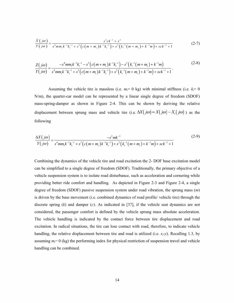
Assuming the vehicle tire is massless (i.e. mt= 0 kg) with minimal stiffness (i.e. kt= 0
N/m), the quarter-car model can be represented by a linear single degree of freedom (SDOF)
mass-spring-damper as shown in Figure 2-4. This can be shown by deriving the relative
displacement between sprung mass and vehicle tire (i.e. ( ) ( ) ( )tX j X j X jω ω ω∆ = − ) as the
following
( )( ) ( )( ) ( )( )
2 1
4 1 1 3 1 1 2 1 1 11t t t t t t
X j s mk
Y j s mm k k s c m m k k s k m m k m sck
ω
ω
−
− − − − − − −
∆ −=
+ + + + + + +
(2-9)
Combining the dynamics of the vehicle tire and road excitation the 2- DOF base excitation model
can be simplified to a single degree of freedom (SDOF). Traditionally, the primary objective of a
vehicle suspension system is to isolate road disturbance, such as acceleration and cornering while
providing better ride comfort and handling. As depicted in Figure 2-3 and Figure 2-4, a single
degree of freedom (SDOF) passive suspension system under road vibration, the sprung mass (m)
is driven by the base movement (i.e. combined dynamics of road profile/ vehicle tire) through the
discrete spring (k) and damper (c). As indicated in [37], if the vehicle seat dynamics are not
considered, the passenger comfort is defined by the vehicle sprung mass absolute acceleration.
The vehicle handling is indicated by the contact force between tire displacement and road
excitation. In radical situations, the tire can lose contact with road, therefore, to indicate vehicle
handling, the relative displacement between tire and road is utilized (i.e. xt-y). Recalling 1.3, by
assuming mt= 0 (kg) the performing index for physical restriction of suspension travel and vehicle
handling can be combined.

15
Figure 2-3: Rendition of SDOF Mercedes- Benz S class front suspension under road- excitation
[12].
Figure 2-4: SDOF base excitation model.
2.1.1. Electro- Mechanical Analogy
To demonstrate the equivalent dynamics provided by the power electronics converter (in
the electrical domain), a mechanical-electrical analogy is adopted. In this work, mechanical force
is considered as the dual of electrical current, whereas speed (velocity) is the dual of voltage.
Referring to a single harmonic base excitation mass-spring-damper model shown in Figure 2-4,
one can apply the mechanical-electrical analogy and converter it into a current source driven
parallel RLC resonance circuit as shown in Figure 2-5 (b).

16
Figure 2-5: Equivalent RLC circuit of a base- excited mass- spring damper model.
The dynamic equation of a parallel RLC circuit in Figure 2-5 is obtained by noting that
the total current iin is the sum of currents flowing through inductor (L), resistor (R), and capacitor
(C) as follows
( ) ( ) ( ) ( )1 1in
dV tC L V t dt R V t i t
dt
− −+ + =∫
(2-10)
Similarly, the road force froad of the base excitation model is the sum of forces acting on spring
(k), sprung mass (m), and damper (c). Thus, the base excitation dynamic equation is given by
( ) ( ) ( ) ( )2
2
2 sin
road
d z t dz tm kz t c f t
dtdt
A tω ω
+ + =
=−
(2-11)
where z=x-y is the sprung mass relative displacement, A is the excitation amplitude, and ω is the
angular frequency. Comparing (2-10) to (2-11) it follows that the electrical voltage, inductance,
resistance, and capacitance are essentially equivalent to relative velocity, inverse stiffness, inverse
damping, and sprung mass of the base excitation model as tabulated in Table 2-1. Therefore, both
equations essentially demonstrate the same response if the current source equals to road force,
iin(t) = -Aw2sinωt.

17
Table 2-1: Adopted electro- mechanical analogy
Mechanical Electrical
Force F Current
Relative velocity zɺ Voltage
Relative displacement z Flux
Stiffness k Inverse inductance: L-1
Damping c Inverse resistance: R-1
Mass m Capacitance: C
To analyze the response of a single degree of freedom (SDOF) base excitation model, it
is prevalent to consider the case of constant amplitude harmonic excitation (i.e. ( ) j tz s z e ω= and
( ) j ty s y e ω= ) [47]- [48]. Applying Laplace transformation to (2-3) with x=xt we can solve for
sprung mass absolute acceleration ( ) ( )1x yω ω−ɺɺ ɺɺ in Laplace domain as the following
( )( )( )
( ) ( )( )
22 2
2 22acc
k cH
k m c
ω ωω
ω ω
+=
− +
.
(2-12)
The relative acceleration ( ) ( )1x yω ω−ɺɺ ɺɺ and displacement ( ) ( )1z yω ω−
ɺɺ transfer functions are
also derived as follows
( )( ) ( )( )
2
_2 22
rel disp
mH
k m c
ωω
ω ω=
− +
(2-13)
( )( ) ( )( )
_2 22
rel acc
mH
k m c
ωω ω
=− +
(2-14)

18
Next, let us on-dimensionalize the transfer functions by defining ( )0.51
n kmω −= ,
( ) 12 nc mξ ω −
= and 1
nr ωω−= . Hence, the transfer functions of sprung mass absolute acceleration,
relative acceleration and displacement are as follows
( ) ( ) ( )( )1
22 2 2 2 2 21 4 1 4acc nH r r r rω ξ ξ
−−= + − +
(2-15)
( )( )( )
2
_2
2 2 21 4rel disp
rH r
r rξ=
− +
(2-16)
(a)
(b)
Figure 2-6: Non-dimensionalized frequency response of (a) sprung mass absolute acceleration (b)
suspension relative displacement.
In order to observe suspension dynamics under different excitation frequencies, we can
generate frequency response functions (FRF) for absolute acceleration and relative displacement,
as shown in Figure 2-6, with transfer functions in non-dimensionalized form. Again, assuming
harmonic excitations, the ideal speed of a vehicle can be written as
( ) 12v lω π
−= (2-17)

19
where ω and l are the excitation angular frequency and distance of travel (road wavelength). As
indicated in (2-12), a larger value of r represents faster vehicle speed. As shown in Figure 2-6 (a),
the mass absolute acceleration frequency response indicates that in the post-resonance frequency
region where frequency ratio r > 2 the absolute acceleration is inverse proportional to the
damping ratio ζ. In contrast, in the region where frequency ratio r < 2 the absolute acceleration
is proportional to damping ratio ζ. As shown in Figure 2-6 (b), the relative displacement response
indicates that the response is inversely proportional to ζ for the entire range of frequencies and the
resonance frequency is inversely proportional to ζ. The higher value of ζ indicates lower levels of
relative displacements. Therefore, it is realized that under constant amplitude harmonic
excitation, the passive suspension with higher value of damping results in better vehicle handling
(i.e. lower relative displacement), while a lower value of damping will contribute to more
comfortable ride in the region where frequency ratio r > 2 due to lower absolute accelerations.
2.1.2. Analytical Analysis of Forced Oscillator with Nonlinear Stiffness
In this section, to illustrate the nonlinear oscillation phenomenon of cubic stiffness force,
so-called Duffing’s equation is solved using a perturbation method (e.g. methods of multiple-
scales, averaging, and Lindstedt Poincare method). To analytically solve the Duffing’s equation
we consider a general forced oscillation of a sprung-mass attached to a nonlinear spring under the
influence of slight viscous damping so that the equation of motion has the following form
2 32 ( )ox x x x E tω εµ εα+ + + =ɺɺ ɺ (2-18)
where ( ) cos cosE t K t k tε= Ω = Ω is the external excitation, ε, µ, and α indicate the level of
nonlinearity, damping and spring constant in the system, respectively. To start analyzing the
system under primary resonance, a detuning parameter σ should be introduced, which
quantitatively describes the nearness of oω εσΩ= + to oω . In a linear undamped system, the
systems response will present unbounded oscillation when being excited at the natural frequency
(i.e. 0σ = ) regardless of how small the excitation amplitude, K. However, in actual events the
amplitude of the system response, even when excited at oω , will be limited by the system’s

20
implicit nonlinearities and damping. Therefore, to offer a uniformly approximation to the system,
one has to make excitation amplitude, K, a function of system nonlinearity,ε , as K kε= . Note
that this arrangement is still consistent with the theories of linear lightly damped system, which
indicates that under small excitation the system’s response becomes unbounded as time
approaches infinity [49].
Here, we assumed the sprung mass response, in (2-18), the form of following
2
0 0 1 1 2 2( ) ( ) ( )x x T x T x Tε ε= + + (2-19)
where oT t= (i.e. normal scale) and 1T tε= (i.e. slow scale, T2 runs slower than T1, which is
omitted in this derivation). Substitute (2-19) into (2-18) while separating terms with ε0 and ε
1 as
follows:
0 2
0 0 0: 0D x xε + =
(2-20)
0 0
1 2 2 3
0 1 1 0 1 0 0 0 0 0 1: 2 2 cos( )D x x D D x D x x k T Tε ω µ α ω σ+ = − − − + + (2-21)
where 1st and 2
nd order derivate operators are
0 1
0 1
... ...d
D Ddt T T
ε ε∂ ∂
= + + = + +∂ ∂
and
22
0 0 122 ...
dD D D
dtε= + + , respectively. Also, ε, µ, and α indicate the level of nonlinearity,
damping and spring constant in the system, respectively. Applying the method of multiple scales
the solutions to (2-19) is expected to be in the form of 0 0 0 0
0 1 1( ) ( )T Tj jx A T e A T e
ω ω−= + , where
1( )A T and 1( )A T are complex conjugates. Substituting it into (2-21) will result the following,
0
1 2 2 2
0 1 1 0
3
0 0 1
: 2 ( ) 3 exp( )
1exp( 3 ) exp( ) ...
2
o o
o o
D x x j A A A A j T
A j T k j T j T
ε ω ω µ α ω
α ω ω σ
′ + = − + +
− + + +
(2-22)
To eliminate the secular term, we set the coefficients of 0exp( )oj Tω to 0, which is the
following,

21
2
1
12 ( ) 3 exp( ) 0
2o
j A A A A k j Tω µ α σ′ − + + + =
(2-23)
Assuming the solution of (2-23) in polar form with 0.5 jA ae β= and grouping the real and
imaginary part one will arrive in a pair of first order ordinary differential equation (ODE),
1
1sin( ) 0
2 o
ka a Tµ σ β
ω′+ − − =
(2-24)
3
1
3 1cos( ) 0
8 2o o
ka a T
αβ σ β
ω ω′− + − =
(2-25)
Note when the motion of the system is under steady state the time derivative of a and β (i.e. a′
and 'β ) are both zero, meaning both amplitude and phase are not changing with respect to time
as indicated by in Figure 2-7.
Figure 2-7: Variation of a and γ (ao =1, γo=1) with T1 for σ=0.05, f=0.5, µ=0.1
Therefore, under steady- state the following occurs
1
1sin( )
2 o
ka Tµ σ β
ω= −
(2-26)
0 20 40 60 80 100
0
0.2
0.4
0.6
0.8
1
1.2
T1 (sec)
Amplitude
a
γ

22
3
1
3 1cos( )
8 2o o
ka T
ασ β
ω ω=− −
(2-27)
Transforming from non-autonomous to autonomous system one can assume 1Tγ σ β= − , thus,
1γ σ β′ ′= − , so (2-26)-(2-27) will lead to (2-28)-(2-29), respectively, as shown in the following
1sin( )
2 o
ka aµ γ
ω′ = − +
(2-28)
33 1cos( )
8 2o o
ka a a
αγ σ γ
ω ω′ = − +
(2-29)
The stability of the steady state motion can be analyzed by obtaining the Jacobian matrix
(i.e., derivative with respect to a and γ) of (2-28)-(2-29), which results in
2
2
3( )
8det 0
1 9( )
8
o
o
da da aa
da d
d a d
da a d
αλ µ λ σ
γ ω
γ α γσ λ µ λ
ω γ
′ ′ − = − − = − −
= ′ ′
= − − = − −
(2-30)
Taking the determinant of the matrix, we obtain2 2
2 2 3 92 ( )( ) 0
8 8o o
a aα αλ µλ µ σ σ
ω ω
+ + + − − =
,
hence the steady state motion is stable when
2 22 3 9
( )( ) 08 8o o
a aα αµ σ σ
ω ω+ − − > . Squaring and
adding (2-28) and (2-29) one will arrive in the following assuming under steady state (i.e.
, 0a γ′ ′ = ),
22
2 2 2
2
3
8 4o o
ka a
αµ σ
ω ω
+ − =
(2-31)
Rearranging above one will be able to obtain the so-called “frequency response equation”
as seen in the following
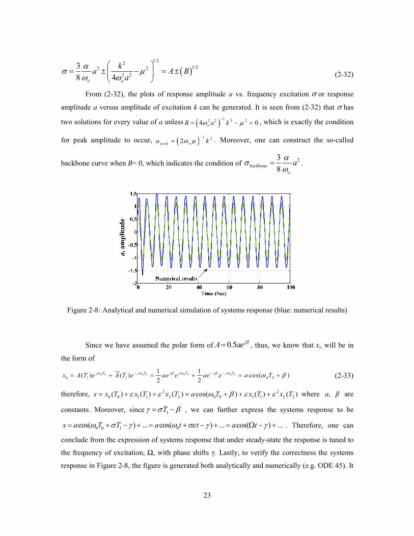
23
( )1/2
21/22 2
2 2
3
8 4o o
ka A B
a
ασ µ
ω ω
= ± − = ±
(2-32)
From (2-32), the plots of response amplitude a vs. frequency excitation σ or response
amplitude a versus amplitude of excitation k can be generated. It is seen from (2-32) that σ has
two solutions for every value of a unless ( ) 12 2 2 2
4 0oB a kω µ−
= − = , which is exactly the condition
for peak amplitude to occur, ( ) 12
2peak oa kω µ−
= . Moreover, one can construct the so-called
backbone curve when B= 0, which indicates the condition of 23
8backbone
o
aα
σω
= .
Figure 2-8: Analytical and numerical simulation of systems response (blue: numerical results)
Since we have assumed the polar form of 0.5 jA ae β= , thus, we know that xo will be in
the form of
0 0 0 0 0 0 0 0
0 1 1 0 0
1 1( ) ( ) cos( )
2 2
T T T Tj j j j j jx A T e A T e ae e ae e a Tω ω ω ωβ β ω β− − −= + = + = +
(2-33)
therefore, 2 2
0 0 1 1 2 2 0 0 1 1 2 2( ) ( ) ( ) cos( ) ( ) ( )x x T x T x T a T x T x Tε ε ω β ε ε= + + = + + + where
a, β
are
constants. Moreover, since 1Tγ σ β= − , we can further express the systems response to be
0 0 1 0cos( ) ... cos( ) ... cos( ) ...x a T T a t t a tω σ γ ω σε γ γ= + − + = + − + = Ω − + . Therefore, one can
conclude from the expression of systems response that under steady-state the response is tuned to
the frequency of excitation, Ω, with phase shifts γ. Lastly, to verify the correctness the systems
response in Figure 2-8, the figure is generated both analytically and numerically (e.g. ODE 45). It

24
is seen that there are consistent deviations in waveform amplitudes under steady-state with
negligible phase differences. This verifies that the first order expansion of Duffing’s equation
using the method of multiple scales is able to predict the systems response with some error
margin.
2.1.3. Electric Generator with Shunt Resistor
Before modeling the regenerative suspension system it is imperative to observe power
generation by a DC machine. Since a DC motor is essentially a mechatronic device, we shall
analyze it in both mechanical and electrical domain. Referring to Figure 2-9, a load resistor is
connected in parallel to the DC generator. The term Tsuspension is the input torque applied at the
motor shaft and Te= ktiin is the developed torque due to iin by multiplying the motor torque
constant kt. In short, when attaching a DC machine to a linearly excited MSD system the
following occurs for power regeneration. As the motor shaft spins purse sinusoidally, it results to
a sinusoidal EMF, which can be seen as an angular velocity controlled voltage source. According
to value of Rload, in Figure 2-9, it leads to different values of iin, and thus the electrically generated
torque Te. Subsquently, the electrically generated Te can be fed back to the MSD system to vary
the desired dynamics. This process integrates the dual purposes of Rload, which achieves both
electrical energy harvesting and mechanical dynamic control. Traditionally, mechanical dashpots,
tunable MR damper, or active-control type hydraulic actuators are not able to achieve both
purposes simultaneously.
Figure 2-9: Electric generator in parallel connection to resistive load.

25
Figure 2-10: Equivalent circuit of electric generator in parallel connection to resistive load.
Applying Newton’s second law of motion to the rotational shaft of DC machine will
result in the following
2
2suspension e
dT T J
dt
θ− =
(2-34)
where J is the rotor inertia, θ is the rotational displacement. By replacing the DC generator with
an equivalent circuit as shown in Figure 2-10 and applying Kirchhoff’s voltage laws (KVL) one
will have the following
( )int int
in
emf in load
diV i R R L
dt= + +
(2-35)
where Rint and Lint represent the dynamics of DC motor internal impedance. The back EMF is
developed by angular velocity θɺ multiplying the motor velocity constant kv as follows
emf vV k θ= ɺ . (2-36)
Substituting (2-34) into (2-35), the dynamic equations of the electric generator with a resistive
load can be written as the following
(2-37)
Assuming zero initial conditions and applying Laplace transformation, we can write
( )2 2intint
2 2
load
v suspension suspension
t t
R RLd d d dk T J T J
dt k dt dt k dt
θ θ θ+ − − = −

26
.
(2-38)
Therefore, the equivalent rotational damping (N-sec/m) and stiffness (N/m) for an electric
generator connected to a load resistor are given by (s=jω)
(2-39)
. (2-40)
It is assumed internal impedance is resistive (i.e. ωLint<< Rint) due to low excitation frequency,
contributed by road irregularities. With the assumption, the equivalent rotational stiffness can be
approximated to zero and the rotational damping can be simplified to k≈0 and
( ) 1
intv t loadc k k R R−
= + .
( )2
int int
2
t vsuspension
load
k k sT Js
R R sL
Js cs k
θ
θ θ θ
= + + +
= + +
( )( )
int
2 2 2
int int
v t load
load
k k R Rc
R R w L
+=
+ +
( )
2
int
2 2 2
int int
v t
load
k k w Lk
R R w L=
+ +

27
2.2. Regenerative Suspension Prototype Modeling
The proposed quarter-car (i.e. Q-car) regenerative suspension prototype is shown in
Figure 2-11. It is modeled as a 1-DOF dynamic system attached to a ball- screw/ DC motor for
energy regeneration. The operation principle of the regenerative suspension is as follows. As the
base is excited, the ball nut experiences linear force with respect to the suspension relative
displacement and velocity. Converting the direction of motion, the screw shaft (coupled to the DC
machine) experiences a bi-directional rotation. Recalling (2-36), it results in sinusoidal EMF,
which can be used for energy regeneration. The dynamics of the sprung mass system are given by
eq f b roadm z kz c z F F+ + + =ɺɺ ɺ (2-41)
where z is the relative displacement between base and sprung mass (i.e. z x y= − ); meq is the
equivalent sprung mass; k is the physical spring coefficient; cf is the physical friction coefficient;
Fb is the equivalent force provided by ball screw, gearbox, DC motor/ generator , and load
resistor Rload. The sprung mass dynamic equation, including the motor dynamics, can be
expressed in detail as follows
( )( ) ( )( )( ) ( )( )
2
2
122 2 2 -2
int int int
122 2 2 -2
int int int
2 sin
m g g b
f
e t g load load
e t g load
J k J Jm z c z kz
d
k k k R R R R L d z
k k k L R R L d z
m Y t
ω
ω ω
ω ω
−
−
+ ++ + +
+ + + +
+ + +
=
ɺɺ ɺ
ɺ
(2-42)
where Y and ω= 2πf are the excitation amplitude and angular frequency; m is the sprung mass;
d=l/2π is the screw lead linear- rotational ratio for torque-force conversion and l is lead ratio of
the ball- screw; Jb is the ball-screw translational mass; Jm and Jg are the motor and gearbox inertia,
respectively; the back EMF and torque constants of the DC machine are indicated by ke and kt,
respectively; the planetary gear ratio is represented by kg, where it is implemented for torque/
angular velocity amplification on its’ input/output terminals, respectively; and the DC machine

28
winding loss and armature inductance are represented by Rint and Lint, respectively. Assuming
int0Lω ≈ the equivalent force Fb is given by
( ) ( )( ) 12 2 2 2
intm g g b e t g loadJ k J J d z k k k R R d z−− −+ + + +ɺɺ ɺ . (2-43)
Figure 2-11: Regenerative suspension 1-DOF dynamic model.
Table 2-2: Equivalent mass, damping coefficient and excitation amplitude.
Symbol Description
+
+ +
+
+
As indicted in Figure 2-11 and Table 2-2, the load resistor Rload, connected to DC machine
terminals, provides equivalent damping force in the electrical domain. In this work, the purpose

29
of the proposed converter is to synthesize a variable Rload to achieve variable equivalent damping
force by absorbing the corresponding power in the electrical domain. The equivalent mass,
damping coefficient and excitation amplitude in terms of other physical parameters values are
listed in Table 2-2. It is worthy to note that equivalent mass meq combines linear mass and
rotational inertia, equivalent damping coefficient (i.e. ceq= cf+ ce) combines both friction terms
and electrical damping, synthesized by attached power electronics, which will be studied in later
sections. The term Yt represents the amplitude of sprung mass acceleration.
2.2.1. Regenerative Suspension Prototype
A 1-DOF regenerative suspension system, fabricated at the Intelligent Vehicles Lab at
Simon Fraser University, is shown in Figure 2-12. The vibrational test-bed setup was developed
to provide experimental verification of equivalent damping synthesis provided by the AC/DC
converter, which will be presented in this Chapter. The electromagnetic-based suspension
generates available AC power when placed under base excitation. As depicted, the 1-DOF
quarter-car system prototype consists of a mass plate on bearings and four parallel springs. A
MTS Hydraulic Actuator (Series 248) was utilized as an actuator to provide base excitation to the
suspension system. A Maxon DC series motor (RE40-218011), attached to a planetary gearhead
(GP52C-223083), was adopted to replace a traditional damper. A high helix lead THK ball-screw
(KX-10) was connected to the DC motor for converting the vertical movement into the rotary
motion. According to [50], the running efficiency of KX-10 can be assumed to be higher than
90%.

30
Figure 2-12: Electromagnetic suspension prototype test bed.
(a)

31
(b)
Figure 2-13: Experimental frequency response of (a) amplitude of relative displacements and (b)
absolute acceleration with respect to various physical load resistors (Ω). Undamped natural
frequency ≈ 6 Hz.
In addition, string potentiometers with spring loaded cable from Celesco SP212 were
used for measuring the suspension relative displacement. The sprung mass acceleration was
measured by 3-axis low power Analog Device ADXL- 326 accelerometers. The main parameter
values of the experimental setup are tabulated in Table 2-4. Recalling Figure 2-11, various
physical power resistors are attached to the terminals of DC machine for the generation of
frequency responses (for excitation frequencies in the range: 2- 9 Hz) in terms of both suspension
relative displacement and sprung mass absolute acceleration are shown in Figure 2-13. As
indicated by Table 2-3 the selected resistance values is capable of applying equivalent damping in
the electrical domain ranging from under to over- damped conditions (i.e. ξ= 0.059 to 1.46).
Table 2-3: Applied damping ratios to electromagnetic suspension prototype with respect to
various load resistors.
Load resistors (Ω) Damping ratio ξ Load resistors (Ω) Damping ratio ξ
10 1.46 60 0.42
20 0.98 80 0.33
30 0.73 100 0.27
40 0.59 120 0.23

32
50 0.49 250 0.11
490 0.059
Table 2-4: Regenerative suspension experimental parameter values
Parameter Value Parameter Value
Sprung mass 16 kg DC motor internal resistance 10 Ω
Total spring constant 23548 N/m Gear ratio of the gearhead 12:1
Rotor inertia of the DC motor 120 g-cm2 Lead ratio of the ball screw l 60 mm/rev
DC motor torque constant 170 mNm/A Travel length of the ball screw 300mm
Accelerometer sensitivity ≈57 mV/g Potentiometer gain ≈3.93 V/m
2.3. Regenerative Power Electronics Topologies
Various types of energy harvesting systems have been reported in the literatures.
Recently, regenerative suspension systems have become extremely popular for dual purposes of
active suspension control and power regeneration. Several topologies of tubular electromagnetic
based regenerative suspension mechanism incorporating permanent magnets have been proposed
[52]- [55]. To harvest the ambient vibration energy, several converters have been proposed [56]-
[58]. In [59], a piezoelectric-based energy harvester was presented by utilizing a buck and buck-
boost converter. The method of impedance matching for maximum power transfer in a
piezoelectric-based energy transducer was presented in [60]. A flyback converter with maximum
power point tracking capability was presented in [61]. A MOSFET-based voltage doubler
coupled with a boost converter was proposed in [62] for low voltage energy harvesting
applications. In [63]-[64], the concept of energy harvesting by providing an equivalent damping
was presented by utilizing a full-bridge rectifier and a DC/DC converter.
Larger scale electromagnetic type transducers have recently gained attention in the
implementation of regenerative vehicular suspension systems and seismic structure dynamic
suppression [52]. In this type of application, the power level (> 1W) is much higher than that of
piezoelectric based converters (< 100 mW). Various types of mechatronic systems have been
reported in the literatures along with electromagnetic dampers for regenerative vibration
suppression and energy harvesting [66]-[69]. Permanent magnet based generators for converting
linear reciprocating motion into electric energy were presented in [71]- [72]. A power converter
for larger scale energy harvesters utilizes a synchronous boost rectifier capable of synthesizing

33
constant input resistor for harvesting damped energy was proposed in [72]. The direct AC/DC
converter demonstrated in [74] aims for seismic structure control and energy harvesting using
tuned mass-spring-damper. The work lacks theoretical analysis in converter switch-mode
operation, control, experimental verification, and requires large converter foot print. A DC/DC
converter indicated in [75], for regeneration from an electromagnetic shock absorber, only
included the simulation results of a buck/boost converter, however, various aspects, such as
AC/DC rectification and converter experimental outcomes were not mentioned.
1k
−road
F1
fc−eqm
VCVSCCCS
ini
Figure 2-14: Analogous electrical model of 1-DOF regenerative suspension.
Referring to the adopted regenerative suspension system depicted in Figure 2-11, the
power generated from the base vibration is distributed into mainly three parts: mechanical
friction, electrical loss, and power transferred to load resistor (see Figure 2-11 (b)). To capture
useful power, the amount delivered to the electrical load needs to be maximized. The total current
passing through the electrical load and motor’s internal resistor can be obtained as
( )( ) 1 1
intin e g loadi k k R R d z− −= + ɺ (2-44)
To analyze power regeneration by Rload, a mechanical-electrical analogy is adopted as
shown in Figure 2-11 (b). According to [50] and considering (2-41), the road force, equivalent
mass, physical stiffness, and equivalent damping are analogous to current source, capacitance,
inverse inductance, and inverse resistance in the electrical domain, respectively. The DC machine

34
provides available power to Rload and supplies mechanical torque proportional to the current iin.
Therefore, the DC machine is represented by a current controlled current sink (CCCS) and
voltage controlled voltage source (VCVS) in the mechanical and electrical domains, respectively.
The DC machine back- EMF vx is given by
vx = ( ) 1
e gk k d z−ɺ . (2-45)
The instantaneous electrical power generated by the damper is a function of the relative speed of
the system, which is
( ) ( )2 1 2 2
intinst e g loadp k k R R d z− −= + ɺ . (2-46)
Assuming ( )sinz A tω θ= + , the average power flow per cycle is calculated as
( ) ( ) ( )22 1 2 2
int0.5avg e g loadp A k k R R d zω − −= + ɺ . (2-47)
2.4. Construction of Standardized Road Profiles
The objective of modeling standardized road profile is to obtain the dynamics of vehicle
tires when placed under realistic excitations. According to ISO 8608 [76], the road profiles can be
characterized by power spectral densities Φ (PSD) defined as
( ) ( )w
o
o
− Ω
Φ Ω = Φ Ω Ω
. (2-48)
where wavenumber Ωo = 1 rad/m and w is defined as road waviness, which describes the
reduction of vibration PSD along the angular wave numbers (rad/m). The value of w= 2 has been
widely recognized [78]. Various classes of road roughness are defined by values of Φ(Ωo). As
depicted in Figure 2-15 (a), PSD of road classes B (i.e. 41
µm3/rad) to D (i.e. 4
3 µm
3/rad) have
been delineated.

35
According to [76]- [77], the road profile X is derived by the summation of sinusoidal waveforms
(with size of N), which can be written as the following
( )1 1
sintL N N
i i j i
j i
X A D ψ×
= =
= Ω −∑ ∑ . (2-49)
where N and Nt indicates the number of points taken along the wavenumber axis and in one meter
of road disctance, respectively. The phase Ψi is pseudorandom and normally distributed between
[0 2π]. The vehicle traveled distance is defined by L, which the sampling rate Dj is determined by
the total number of sampling point taken throughout the entire traveled distance (size: L×Nt). The
excitation amplitudes Ai is given by
( )2i iA d= Φ Ω Ω (2-50)
where dΩ is the step size taken from the wavenumbers. Referring to PSD profiles in Figure 2-15
(a), it allows the realization of ISO standard excitation profiles by (2-48)- (2-50). In this case, the
road profiles from class B to D for the distance of 100 (m) has been reconstructed in Figure 2-15
(b). The class C road profiles with nominal values of i=1, 2 and 100, 200 within 100 samples are
depicted in Figure 2-16 (a) and (b), respectively.
Figure 2-15: (a) PSD Φ(Ω) and (b) road profile X (in cm) of ISO 8608 road class B to D.

36
Figure 2-16: Nominal longitudinal class C road profiles with (a) i= 1, 2 and (b) 100, 200 within
100 samples.
Alternatively, according to [78], the road profile can also be constructed, with respect to
temporal excitation frequency, by passing a unit- intensity white noise through a low pass filter
(LPF) expressed as
( )2 r
o
G VG s
s w
π=
+ (2-51)
where Gr= Φ(Ωo)/(2π)2 is the roughness coefficient with Φ(Ωo) expressed in (m
3/ cycle), V is the
vehicle velocity, w= 2πVv is the temporal excitation frequency with wavenumber v in (cycle/m),
and wo= V is the cut-off frequency of the LPF. The instantaneous waveform and amplitude
spectra of a white noise with unit intensity are shown in Figure 2-17. As indicated by (2-51),
higher road class and faster vehicle velocity amplifies the gain and extends the cut-off frequency
of the white noise LPF, which means assuming fixed travel duration higher vehicle velocity and
rougher roads will provide higher available energy.
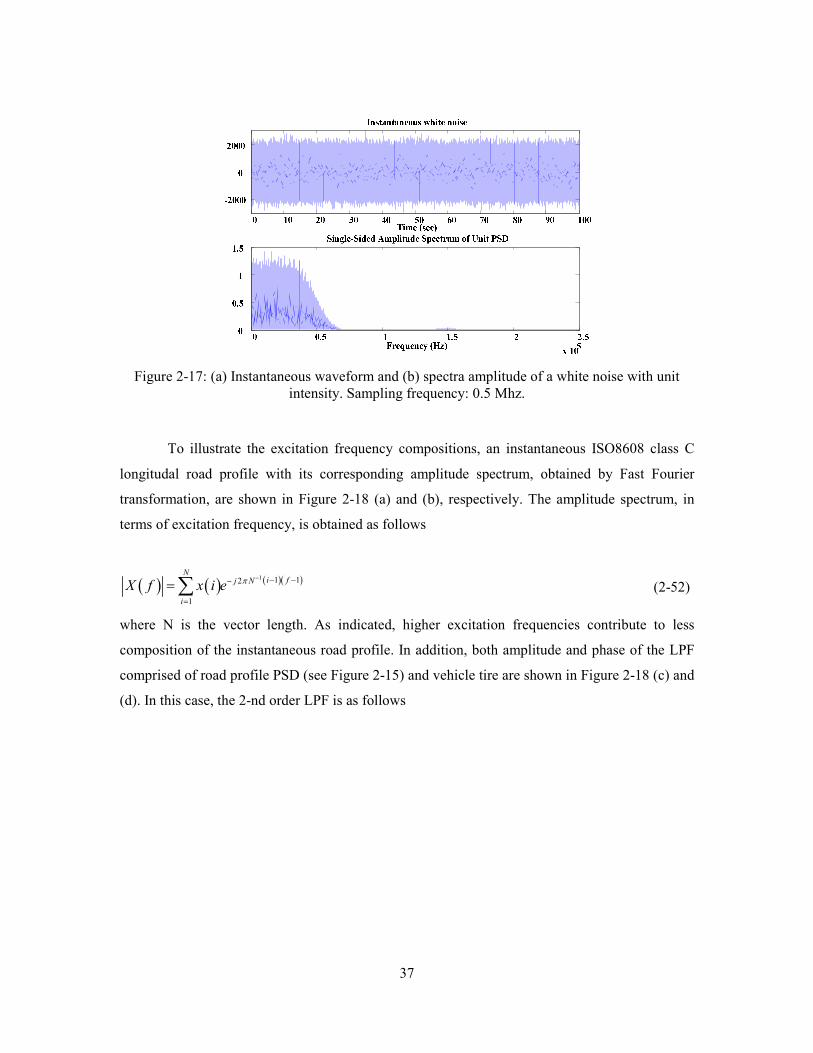
37
Figure 2-17: (a) Instantaneous waveform and (b) spectra amplitude of a white noise with unit
intensity. Sampling frequency: 0.5 Mhz.
To illustrate the excitation frequency compositions, an instantaneous ISO8608 class C
longitudal road profile with its corresponding amplitude spectrum, obtained by Fast Fourier
transformation, are shown in Figure 2-18 (a) and (b), respectively. The amplitude spectrum, in
terms of excitation frequency, is obtained as follows
( ) ( ) ( )( )1 1 12
1
Ni fj N
i
X f x i e π − − −−
=
=∑ (2-52)
where N is the vector length. As indicated, higher excitation frequencies contribute to less
composition of the instantaneous road profile. In addition, both amplitude and phase of the LPF
comprised of road profile PSD (see Figure 2-15) and vehicle tire are shown in Figure 2-18 (c) and
(d). In this case, the 2-nd order LPF is as follows

38
( ) 2
1.26
251.3G s
s s≈
+
(2-53)
Figure 2-18: (a) Class C longitudal road profile in 69.4 (m) and its’ (b) single- sided amplitude
spectrum. Bode plot of combined class C PSD and vehicle tire dynamics in both (c) amplitude
and (d) phase. Note: Sampling frequency= 0.5 MHz.
2.5. Full- sized Vehicle Power Regeneration Potential
Based on the experimental results of a small-scale suspension prototype (to be outlined in
later chapters), one can estimate the available energy distribution and total energy regeneration
under various ISO road classes for full-size vehicles. In this work, to illustriate the power
regeneration potentials, both full-size electric vehicle (e.g. Tesla Model S) and 6-wheeled
recreational vehicle (e.g. Autotrail Frontier Chieftain Motorhome) can serve as suitable examples.

39
According to Figure 2-19 (a), the boundaries “o-b” indicates energy distributions taking
place in a regenerated suspension system, generally. As depicted, the available energy is
comprised of kinetic/ potential, damped, and regenerated energies. The exchange between kinetic
and potential provides sprung mass oscillation, which implies indefinite oscillation when the
damped energy is absent. This also indicates the amount of avaialbe energy that is not
harvestable. The boundary “b- c” indicates energy loss of ball-screw friction and DC motor
armature coil. It is noted the calculation of the ball- screw driving efficiency (or energy loss)
between “b- c” is calculated by forces between moving the ball nut and screw shaft. The
boundaries “c- e” indicates energy distribution in the electrical domain, where charged energy is
obtained by subtracting converter energy loss.
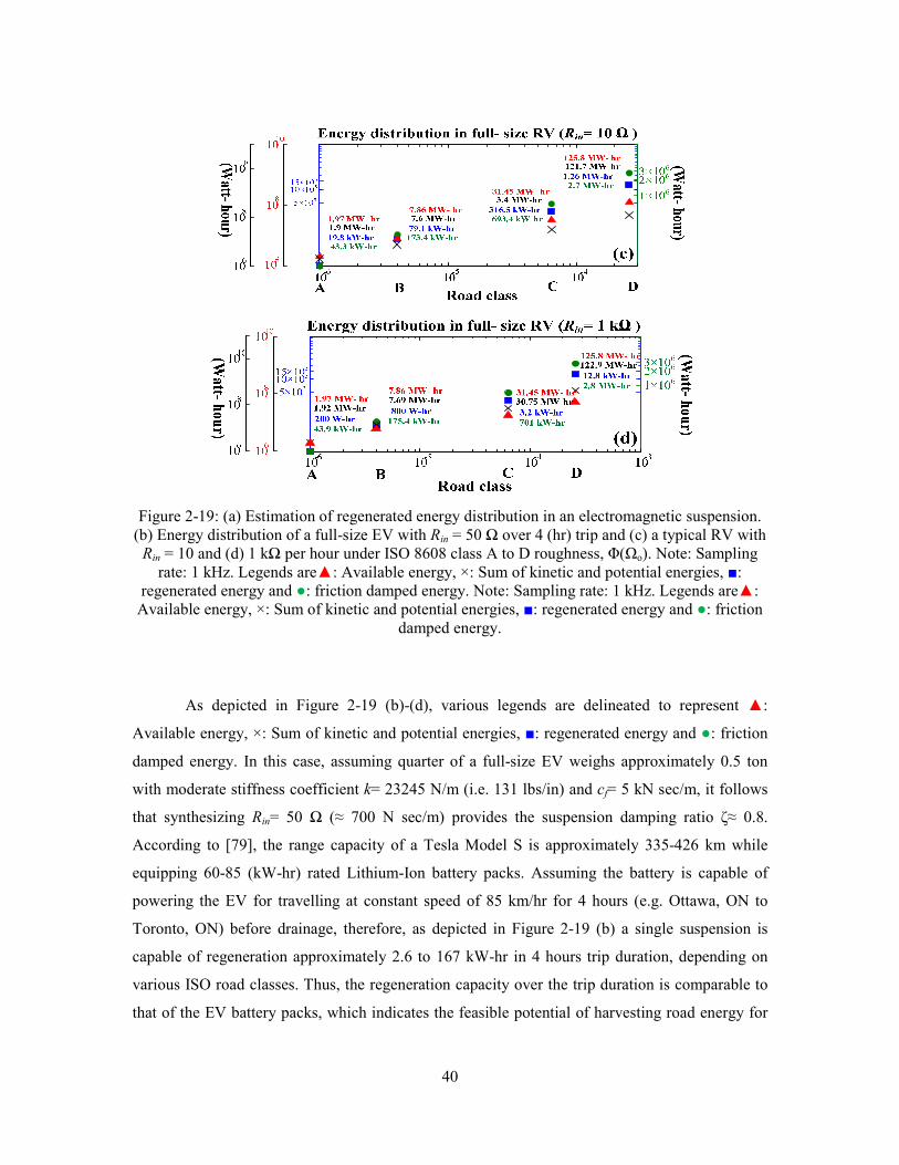
40
Figure 2-19: (a) Estimation of regenerated energy distribution in an electromagnetic suspension.
(b) Energy distribution of a full-size EV with Rin = 50 Ω over 4 (hr) trip and (c) a typical RV with
Rin = 10 and (d) 1 kΩ per hour under ISO 8608 class A to D roughness, Φ(Ωo). Note: Sampling
rate: 1 kHz. Legends are: Available energy, ×: Sum of kinetic and potential energies, :
regenerated energy and : friction damped energy. Note: Sampling rate: 1 kHz. Legends are:
Available energy, ×: Sum of kinetic and potential energies, : regenerated energy and : friction
damped energy.
As depicted in Figure 2-19 (b)-(d), various legends are delineated to represent :
Available energy, ×: Sum of kinetic and potential energies, : regenerated energy and : friction
damped energy. In this case, assuming quarter of a full-size EV weighs approximately 0.5 ton
with moderate stiffness coefficient k= 23245 N/m (i.e. 131 lbs/in) and cf= 5 kN sec/m, it follows
that synthesizing Rin= 50 Ω (≈ 700 N sec/m) provides the suspension damping ratio ζ≈ 0.8.
According to [79], the range capacity of a Tesla Model S is approximately 335-426 km while
equipping 60-85 (kW-hr) rated Lithium-Ion battery packs. Assuming the battery is capable of
powering the EV for travelling at constant speed of 85 km/hr for 4 hours (e.g. Ottawa, ON to
Toronto, ON) before drainage, therefore, as depicted in Figure 2-19 (b) a single suspension is
capable of regeneration approximately 2.6 to 167 kW-hr in 4 hours trip duration, depending on
various ISO road classes. Thus, the regeneration capacity over the trip duration is comparable to
that of the EV battery packs, which indicates the feasible potential of harvesting road energy for

41
further extending the vehicle’s range capacity by at least 12-15% (10.4 kW-hr/60 kW-hr
assuming smooth road, ISO8608 class A, with four regenerative suspensions in 4 hours). This is
equivalent to range extension of 50 to 70 km for the Tesla Model S.
In addition, the total recreational vehicle (RV) mass of roughly 12.5 ton is evenly
distributed to the suspensions while V= 85 km/hr, k= 23245 N/m and cf= 10 kN sec/m, the total of
3.2 to 316.5 (kW- hr) while driving on typical ISO 8608 class C road for one hour can be
obtained by the adopted DC generator/ ball- screw mechanism. It is worthy to note, with cf= 10
kN sec/m, synthesizing Rin= 10 Ω (i.e. ce= 2.28 kNs/m by substituting in Table 2-4) to 1 kΩ (ce=
45.6 Ns/m) represents cases of critically and under damped for the sprung mass dynamics,
respectively. Therefore, according to [80], for a typical 5- hour road trip (e.g. Vancouver, BC to
Osoyoos, BC), on average road condition, the available power provided by the road surface
allows powering the on- board recreational appliances for at least 12 (hr).
2.6. Chapter Summary
In this chapter, models for one and two DOF dynamic systems were obtained to
demonstrate the responses of sprung mass under base excitations. Moreover, the modelling of
ISO 8608 road profiles, for different road roughnesses, was described. The model allows realistic
estimation of road energy harvesting for full-scale vehicles (e.g., full- size sedan and recreational
vehciles). In addition, the power regeneration mechanism of DC machine under road excitation
was investigated. The detailed modeling of a current controlled switched-mode rectifier (SMR),
synthesizing variable electrical dampers, for the purpose of energy harvesting will be presented in
the next chapter.

42
Chapter 3.
Bi- directional Switch Mode Rectifier for Synthesizing
Variable Damping and Semi- Active Control
In this chapter, the concept of using a switch-mode rectifier (SMR) for synthesizing a
variable electrical damper is demonstrated. Along with hysteresis current control, it is shown that
both the amplitude and phase of the converter current can be controlled, with respect to irregular
and stochastic generated back-EMF voltage, which is equivalent to turning the desired
synthesized resistor values. According to the derivations shown previously, this is equivalent to
tuning the mechanical damping coefficient through capturing road-induced vibration energy.
3.1. Converter Modeling
The bi- directional power converter for synthesizing variable resistor is shown in Figure
3-1. The synthesizer is essentially a current controlled switch-mode rectifier (SMR) operating in
the continuous conduction mode (CCM). As depicted, the power stage consists of a physical
power inductor and a single phase Voltage Source Inverter (VSI) for providing the desired 3-
level vc through the corresponding PWM pulses driving the power MOSFETs. Before
synthesizing variable resistors in a switch- mode converter, we consider a general variable
resistor, Rin, shown in Figure 3-2. The value of Rin is determined through the amplitude/phase
relationship between resistor voltage, V(t), and current, i(t) as seen in (3-1). Assuming both V(t)
and i(t) are completely in-phase (i.e., high power factor), varying the ratio between both
waveforms is synonymous to changing terminal resistance R across the terminal “a-b”.
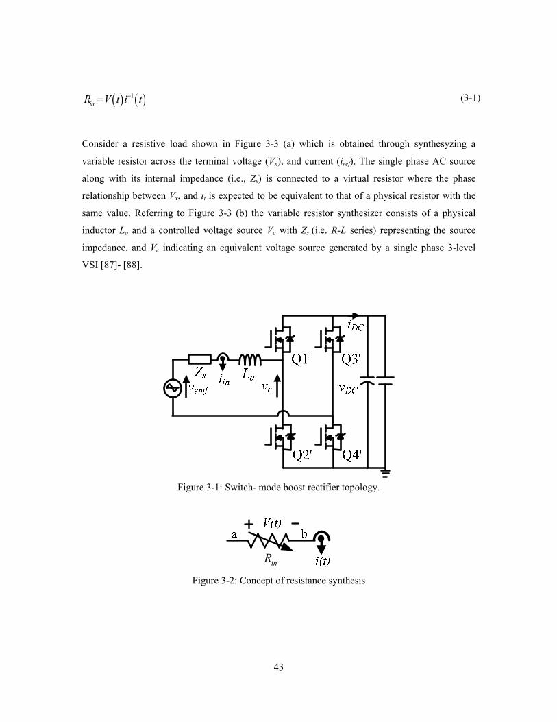
43
( ) ( )1
inR V t i t−= (3-1)
Consider a resistive load shown in Figure 3-3 (a) which is obtained through synthesyzing a
variable resistor across the terminal voltage (Vx), and current (iref). The single phase AC source
along with its internal impedance (i.e., Zs) is connected to a virtual resistor where the phase
relationship between Vx, and it is expected to be equivalent to that of a physical resistor with the
same value. Referring to Figure 3-3 (b) the variable resistor synthesizer consists of a physical
inductor La and a controlled voltage source Vc with Zs (i.e. R-L series) representing the source
impedance, and Vc indicating an equivalent voltage source generated by a single phase 3-level
VSI [87]- [88].
Figure 3-1: Switch- mode boost rectifier topology.
inR
Figure 3-2: Concept of resistance synthesis

44
tvini
(a) (b)
Figure 3-3: Equivalent model of variable resistance synthesis (in Laplace domain variables)
If the driving point impedance at the terminal (shown by “+/-“) in both Figure 3-3 (a) and (b) can
be assumed resistive, the current flowing through both circuits can be equated. Defining the
variables Iin(s) and Iref(s) as Laplace domain representation of terminal current iin and reference
current iref one will obtain the following:
To ensure correct resistor synthesis the expression between source voltage (Vx) and controlled
voltage source (Vc) is derived next. By equating (3-2) to (3-3) the expression of Vc in both time
and Laplace domains can be obtained as the following:
( ) x si
c an
sin
dv R
dv L
ti L
i− −= +
(3-4)
( ) ( )in ac x
s in
R sLV s V s
Z R
−=
+ (3-5)
where Rs and Ls represents the motor internal impedance, Rin is the desired variable resistance and
La is the line inductor. The transfer function indicates the relationship between Vx(s) and Vc(s),
where the amplitude attenuations and phase shifts are determined by values of passive elements.
Thus, by controlling Vc(s) to follow the relationship in (3-5) ensures the correct synthesis of Rin.
( ) ( )xref
s in
V sI s
Z R=
+ (3-2)
( ) ( ) ( )x cin
s a
V s V sI s
Z sL
−=
+ (3-3)

45
3.2. Regeneration and Motoring Modes
The purpose of operating in the regenerative mode is to harvest energy from the
suspension mechanism through the electric machine while providing positive damping force to
the suspension system. In the regenerative (motoring) mode, during positive cycle of line voltage,
positive (negative) source power contributes to storing (dissipating) of DC bus energy (i.e.,
battery). This condition indicates a charging (discharging) operation.
Figure 3-4: Motoring and regeneration states by direction of current.
Figure 3-5: Configuration of regenerative suspension indicating the power converter providing
the desired equivalent dynamics through vx and iin.
Referring to Figure 3-4 and Figure 3-5 the role of power converter is to convert the
kinetic energy, induced by excitation input, to the load battery VDC. Here, we defined the average
harvested power as follows

46
1st T
DC s DC DC
t
P T i v dt
+−= ∫
(3-6)
where Ts is EMF voltage period (i.e. line period), iDC is defined as the charged current, vDC is the
battery voltage . According to Figure 3-3 (b), the average controlled voltage source generated
by a single phase VSI through the following
1swt T
c sw DC
t
v T v dt
+−= ∫
(3-7)
where TSW is the MOSFET switching period. Recalling (3-5), it is also noted the limitation of
SMR in synthesizing variable resistors is limited by Rs. Referring to Figure 3-2 and assuming iin=
iref= Vx(Rin)-1
, theorectically the converter is operating in regeneration mode when Rin>Rs, since in
low operating frequency we can assume c ins
x s x
i
x
n
Rv R vv v
Ri≈ ≈− − . Having Rin>Rs ensures both
vc and vx have the same polarity. Since the purpose of the converter is synthesizing variable
resistors (i.e. resistive behavious at the line terminal), meaning both vc and iin waveforms will be
in- phase, ideally. When Rin< Rs, vc indicates opposite polarity to that of vx, which means both vc
and iin waveforms are out of phase, thus the converter is operating in motoring mode. The
maximum negative synthesized resistor (i.e. Rin< 0 Ω) is limited by the value of battery voltage or
inverter voltage, since + sx
n
c
i
x
Rv
Rv v≈ .
Having the equivalent model of the SMR we are able to model the average battery consumed/
harvested power as the following
1st T
DC s c in
t
P T v i dt
+−= ∫
(3-8)
Again, since torque generated by a DC motor is directly related to its current, thus iin represents
the desired response synthesized in the electrical domain. Recalling (3-4) - (3-5) and assuming
voltage drop between La and Ls is negligible (i.e. a s
in ind dL L
t t
i
d
i
d+ ≈ 0 V) due to low excitation

47
frequency, thus the phase difference between vx and vc is negligible. The amplitude difference is
correlated to the motor/ generator loss since nx sc iv v R i−≈ , meaning, by adjusting the duty cycle
of the VSI according to iin the desired vc can be obtained.
Figure 3-6: Average regenerated power DCP (watts) with Rin= 30 to 100 Ω and vx= 10 sin(20πt).
Hence, for illustration purposes and assuming Rs= 30 Ω, according to the defined
direction of DCP and Figure 3-6, it indicates power charging (i.e. regeneration mode) when Rin≥ Rs.
It is noted as Rin increases the amount of average harvested power decreases, when Rin≈ Rs leads
to maximum DCP with lower conversion efficiency, which will be shown in details in later
sections. This is a typical trade-off for maximum power transfer. It also shows that in order to
enlarge the range of synthesized Rin (by AC/DC converter) the selection of DC machine in terms
of its equivalent resistor (Rs) coil loss is imperative.
3.3. Hysteresis Current Control
3.3.1. Double- band Three-level Hysteresis Current Control
In this work, a double-band hysteresis current controller (DB- HCC) was implemented to
control iin. The variable sampling frequency modulating scheme is implemented for its wide
bandwidth and fast transient response, unconditional stability [81]-[86], full expandability to

48
multi-level topologies (e.g., flying capacitor, neutral point clamp, cascaded H-bridge topologies
for lower transistor electromagnetic interference EMI/ inverter total harmonic distortion THD),
and accurate line resistor synthesis. The SMR with a controller consists of hysteresis comparators
with two different sizes of error-bands are shown in Figure 3-7. In order to control vc for correct
Rin synthesis the terminal current iin should be regulated to follow iref, as recalled in (3-5). The
controller consists of hysteresis comparators with two different sizes of error-bands as shown in
Figure 3-7 (b). With the desired gating signals for Q1-4, additional digital logic circuits were
introduced for MOSFETs switching frequency (i.e. switching power loss) reduction and
equalization, synonymous to carrier- based PWM modulation [87]- [88]. As a result, the average
switching frequency is given by
( )( ) 10.6 0.5sw DC af v k k L I
−≈ − ∆ (3-9)
where k = vemf/vDC is the modulation index, ∆I is the small error band, and vDC is the inverter input
voltage.
(a)
(b)
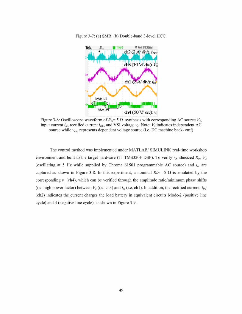
49
Figure 3-7: (a) SMR. (b) Double-band 3-level HCC.
Figure 3-8: Oscilloscope waveform of Rin= 5 Ω synthesis with corresponding AC source Vx,
input current iin, rectified current iDC, and VSI voltage vc. Note: Vx indicates independent AC
source while vemf represents dependent voltage source (i.e. DC machine back- emf)
The control method was implemented under MATLAB/ SIMULINK real-time workshop
environment and built to the target hardware (TI TMS320F DSP). To verify synthesized Rin, Vx
(oscillating at 5 Hz while supplied by Chroma 61501 programmable AC source) and iin are
captured as shown in Figure 3-8. In this experiment, a nominal Rin= 5 Ω is emulated by the
corresponding vc (ch4), which can be verified through the amplitude ratio/minimum phase shifts
(i.e. high power factor) between Vx (i.e. ch3) and iin (i.e. ch1). In addition, the rectified current, iDC
(ch2) indicates the current charges the load battery in equivalent circuits Mode-2 (positive line
cycle) and 4 (negative line cycle), as shown in Figure 3-9.

50
Figure 3-9: State diagram of DB- HCC.
The current ripple is primarily determined by smaller error-band hysteresis comparator
while the large error-band hysteresis comparator is implemented to reverse the polarity of vDC,
when the smaller error-band comparator is unable to regulate the current error. Under this
condition, the larger error-band comparator will activate to accomplish polarity reversal.
Referring to the controller state machine shown in Figure 3-9, it is assumed the converter initially
operates in the regeneration state with sign(vin) >0. The smaller error-band comparator acts as a
single-band hysteresis comparator, which switches on either Q1 or Q2 according to the error
current (i.e., ∆I = iref - iin), defined as the difference between reference current iref and measured
current it. When |iin-iref|< ∆I, Q2/4 are switched on, connecting vin to La, which charges it at the rate
of ∆it = Vx/La. When |iin-iref|> ∆I, Q1/4 are switched on thus iin into battery at the rate of ∆iin = (vx-
VDC)/La. Subsequently, when sign(vin) <0, Q3 will switch on with either Q1 or 2 depending on the
output of the smaller error-band comparator. The large error-band comparator switches on Q3 or
4 for vDC polarity reversal, which takes place when the small error-band lost regulation (e.g.
sign(vin) reversal).
To verify the DB-HCC control law state diagram, Figure 3-10 (a) indicates ierr over duration of 1
(sec). In this case, the nominal small and larger bands are 5 (mA) and 1 (A), respectively.
Essentially, the control method regulates ierr by presenting different values of vc, generated by
VSI. The detailed ierr shows lost regulation of small- band and transitioning of large-band are
depicted in Figure 3-10 (b). The detailed switching mode transitioning clearly demonstrates
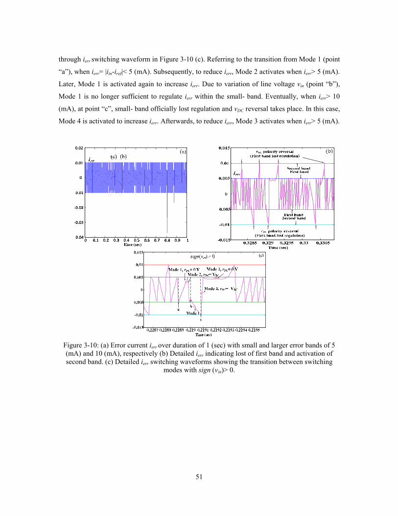
51
through ierr switching waveform in Figure 3-10 (c). Referring to the transition from Mode 1 (point
“a”), when ierr= |iin-iref|< 5 (mA). Subsequently, to reduce ierr, Mode 2 activates when ierr> 5 (mA).
Later, Mode 1 is activated again to increase ierr. Due to variation of line voltage vin (point “b”),
Mode 1 is no longer sufficient to regulate ierr within the small- band. Eventually, when ierr> 10
(mA), at point “c”, small- band officially lost regulation and vDC reversal takes place. In this case,
Mode 4 is activated to increase ierr. Afterwards, to reduce ierr, Mode 3 activates when ierr> 5 (mA).
Figure 3-10: (a) Error current ierr over duration of 1 (sec) with small and larger error bands of 5
(mA) and 10 (mA), respectively (b) Detailed ierr indicating lost of first band and activation of
second band. (c) Detailed ierr switching waveforms showing the transition between switching
modes with sign (vin)> 0.
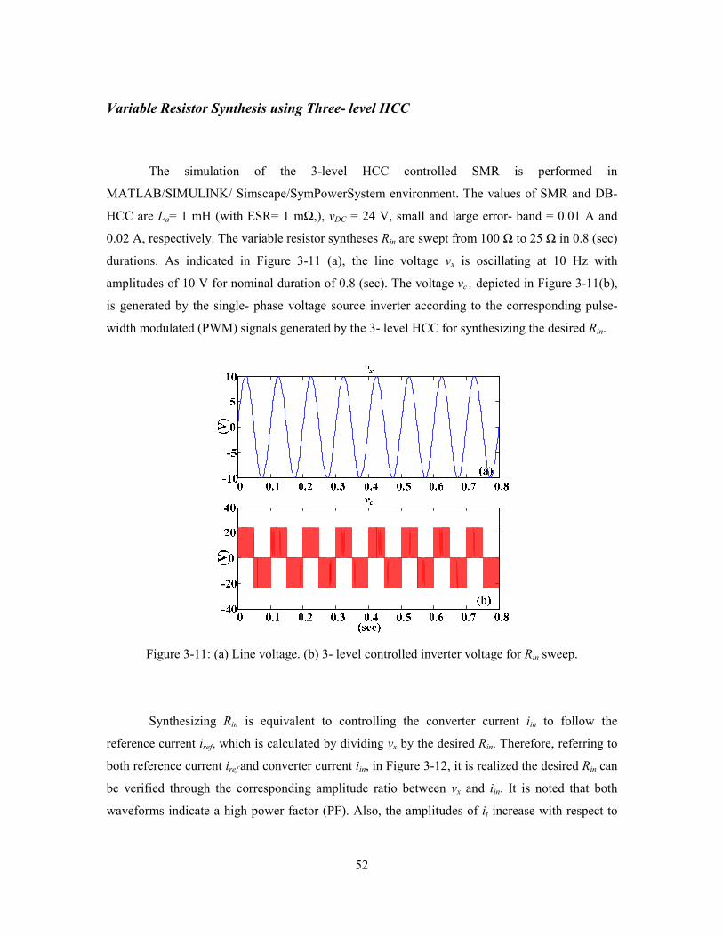
52
Variable Resistor Synthesis using Three- level HCC
The simulation of the 3-level HCC controlled SMR is performed in
MATLAB/SIMULINK/ Simscape/SymPowerSystem environment. The values of SMR and DB-
HCC are La= 1 mH (with ESR= 1 mΩ,), vDC = 24 V, small and large error- band = 0.01 A and
0.02 A, respectively. The variable resistor syntheses Rin are swept from 100 Ω to 25 Ω in 0.8 (sec)
durations. As indicated in Figure 3-11 (a), the line voltage vx is oscillating at 10 Hz with
amplitudes of 10 V for nominal duration of 0.8 (sec). The voltage vc , depicted in Figure 3-11(b),
is generated by the single- phase voltage source inverter according to the corresponding pulse-
width modulated (PWM) signals generated by the 3- level HCC for synthesizing the desired Rin.
Figure 3-11: (a) Line voltage. (b) 3- level controlled inverter voltage for Rin sweep.
Synthesizing Rin is equivalent to controlling the converter current iin to follow the
reference current iref, which is calculated by dividing vx by the desired Rin. Therefore, referring to
both reference current iref and converter current iin, in Figure 3-12, it is realized the desired Rin can
be verified through the corresponding amplitude ratio between vx and iin. It is noted that both
waveforms indicate a high power factor (PF). Also, the amplitudes of it increase with respect to
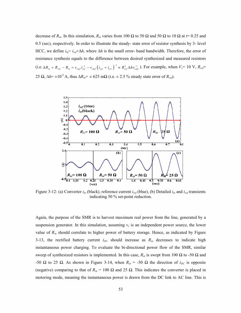
53
decrease of Rin. In this simulation, Rin varies from 100 Ω to 50 Ω and 50 Ω to 10 Ω at t= 0.25 and
0.5 (sec), respectively. In order to illustrate the steady- state error of resistor synthesis by 3- level
HCC, we define iin= iref+∆h, where ∆h is the small error- band bandwidth. Therefore, the error of
resistance synthesis equals to the difference between desired synthesized and measured resistors
(i.e. ( ) 11 2 1
in ref in emf ref emf ref err ref emfR R R v i v i i R hv−− −∆ = − = − + ≈ ∆ ). For example, when Vx= 10 V, Rref=
25 Ω, ∆h= ±10-2
A, thus ∆Rin= ± 625 mΩ (i.e. ± 2.5 % steady state error of Rref).
Figure 3-12: (a) Converter iin (black), reference current iref (blue), (b) Detailed iin and iref transients
indicating 50 % set-point reduction.
Again, the purpose of the SMR is to harvest maximum real power from the line, generated by a
suspension generator. In this simulation, assuming vx is an independent power source, the lower
value of Rin should correlate to higher power of battery storage. Hence, as indicated by Figure
3-13, the rectified battery current iDC should increase as Rin decreases to indicate high
instantaneous power charging. To evaluate the bi-directional power flow of the SMR, similar
sweep of synthesized resistors is implemented. In this case, Rin is swept from 100 Ω to -50 Ω and
-50 Ω to 25 Ω. As shown in Figure 3-14, when Rin = -50 Ω the direction of iDC is opposite
(negative) comparing to that of Rin = 100 Ω and 25 Ω. This indicates the converter is placed in
motoring mode, meaning the instantaneous power is drawn from the DC link to AC line. This is

54
an invaluable feature of the controlled SMR for applications in suspension regenerative semi-
active control schemes, which will be outlined in Chapter 3. Moreover, from Section 2.2, in the
mechanical domain, this indicates the synthesis of negative damping coefficient ce=
2 20.02e t g
k k k d− .
Figure 3-13: DC link charged current for Rin sweep.
Figure 3-14: (a) Converter it (black), reference current iref (blue). (b) DC link current indicating
transition between generating and motoring mode.
3.3.2. Multi- level Hysteresis Current Control
The aforementioned 3- level HCC can be readily expanded to multi-level modulation
schemes. To demonstrate the expandability of HCC, a 5- level HCC cascaded H- bridge has been
simulated in MATLAB/ SIMULINK/SymPowerSystem. It is worthy to mention that comparing
to DB- HCC the benefits of this strategy, in high- power level applications, is to provide lower
MOSFET switching frequency (lower switching loss), EMI, and inverter THD. The apparent

55
drawbacks are larger conduction loss (due to addition MOSFET RDS(on)), converter, and auxiliary
circuit footprints [89]- [93]. During regular conduction modes, the conduction loss is doubled for
a 5-level cascaded H- bridge SMR topology comparing to that of a 3-level SMR.
Before illustrating the control algorithm, it is important to mention that, in this work, with
lower power-levels (< 5 W), the apparent drawbacks of the cascaded topology (i.e. increased
conduction loss, larger converter foot- print) exceed the potential benefits (i.e. EMI, THD
reductions) due to low DC bus voltages. Due to this reason, the prototype of the 5- level SMR
was not fabricated.
As depicted in Figure 3-15, the 5- level SMR topology is synonymous to that of a 3- level
SMR with an additional H- bridge. It is worthwhile to note the double- band type HCC control
algorithm is an expansion to that of a 3- level control law (see Figure 3-9). Since, a single- bridge
topology can only generate 3 voltage levels (i.e. -vDC, 0, vDC). As a result, the state machines of 3-
level HCC have to be expanded. Referring to Figure 3-16, there are 5 states exist in a 5- level
HCC state machine. With the states transitioning to the other represents the voltage change
generated by the cascaded topology.
Figure 3-15: Five- level cascaded H- bridge SMR.
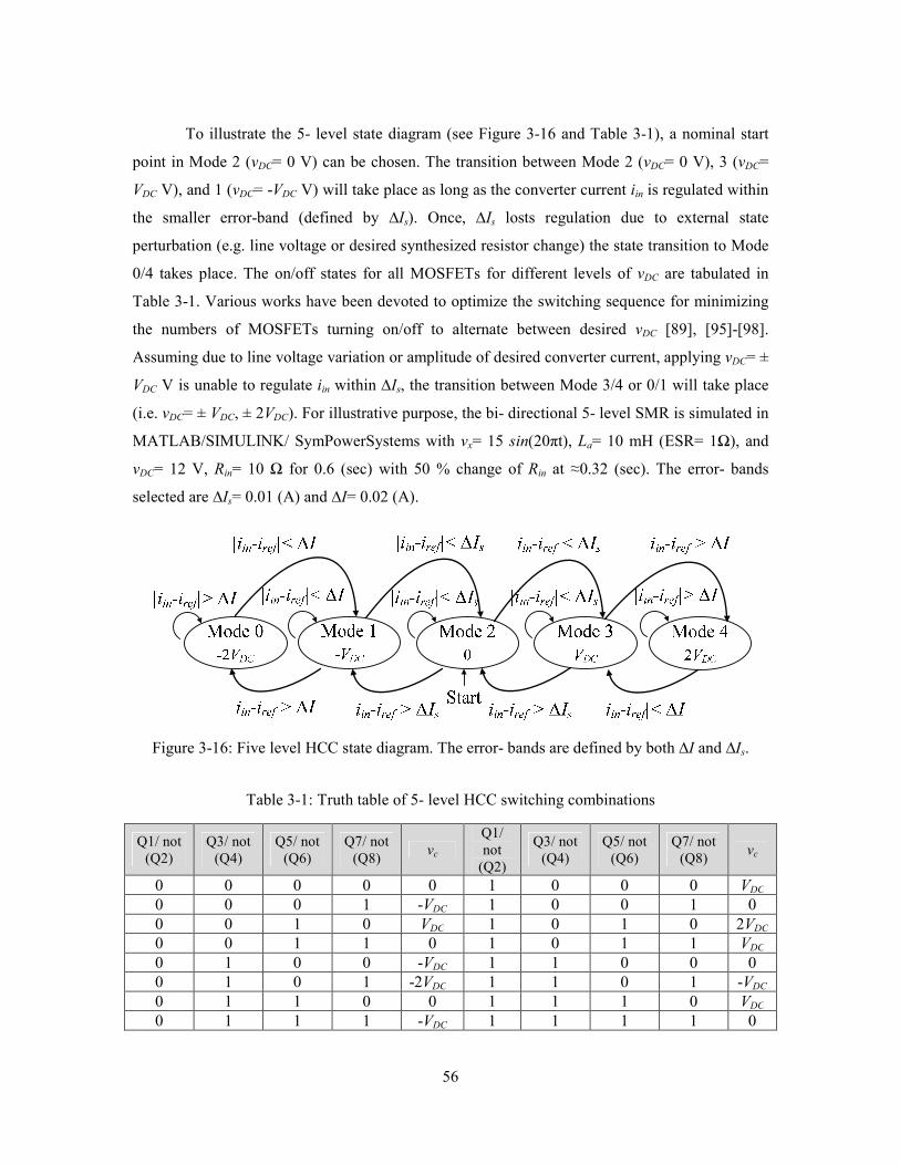
56
To illustrate the 5- level state diagram (see Figure 3-16 and Table 3-1), a nominal start
point in Mode 2 (vDC= 0 V) can be chosen. The transition between Mode 2 (vDC= 0 V), 3 (vDC=
VDC V), and 1 (vDC= -VDC V) will take place as long as the converter current iin is regulated within
the smaller error-band (defined by ∆Is). Once, ∆Is losts regulation due to external state
perturbation (e.g. line voltage or desired synthesized resistor change) the state transition to Mode
0/4 takes place. The on/off states for all MOSFETs for different levels of vDC are tabulated in
Table 3-1. Various works have been devoted to optimize the switching sequence for minimizing
the numbers of MOSFETs turning on/off to alternate between desired vDC [89], [95]-[98].
Assuming due to line voltage variation or amplitude of desired converter current, applying vDC= ±
VDC V is unable to regulate iin within ∆Is, the transition between Mode 3/4 or 0/1 will take place
(i.e. vDC= ± VDC, ± 2VDC). For illustrative purpose, the bi- directional 5- level SMR is simulated in
MATLAB/SIMULINK/ SymPowerSystems with vx= 15 sin(20πt), La= 10 mH (ESR= 1Ω), and
vDC= 12 V, Rin= 10 Ω for 0.6 (sec) with 50 % change of Rin at ≈0.32 (sec). The error- bands
selected are ∆Is= 0.01 (A) and ∆I= 0.02 (A).
Figure 3-16: Five level HCC state diagram. The error- bands are defined by both ∆I and ∆Is.
Table 3-1: Truth table of 5- level HCC switching combinations
Q1/ not
(Q2)
Q3/ not
(Q4)
Q5/ not
(Q6)
Q7/ not
(Q8) vc
Q1/
not
(Q2)
Q3/ not
(Q4)
Q5/ not
(Q6)
Q7/ not
(Q8) vc
0 0 0 0 0 1 0 0 0 VDC
0 0 0 1 -VDC 1 0 0 1 0
0 0 1 0 VDC 1 0 1 0 2VDC
0 0 1 1 0 1 0 1 1 VDC
0 1 0 0 -VDC 1 1 0 0 0
0 1 0 1 -2VDC 1 1 0 1 -VDC
0 1 1 0 0 1 1 1 0 VDC
0 1 1 1 -VDC 1 1 1 1 0

57
As depicted in Figure 3-17, the line voltage vx, in Figure 3-17 (a), is assumed an
independent AC voltage source. The converter current iin, in Figure 3-17 (b), varies corresponding
to the desired Rin. The error current ierr= iref -iin and controlled cascaded H- bridge voltage are
shown in Figure 3-17 (c) and (d), respectively. To observe the state transition, a detailed depiction
of the waveforms is placed in Figure 3-18. As shown in Figure 3-18 (d) the state transition takes
place from Mode 2 to 4 due to the lost regulation of ∆Is. According to (3-3)- (3-4), since the
maximum voltage (at 100% duty cycle) can be generated by a single H- bridge is vc= VDC,
therefore, when the voltage level is incapable of regulating the reference current iref (for
synthesizing Rin) the transition will take place in the larger error-band. The larger error- band is
defined by ∆I.
Figure 3-17: (a) Line voltage, (b) converter current, (c) error current, and (d) inverter generated
voltage. vx= 15 sin(20πt) and vDC= 12 V.

58
Figure 3-18: Detailed (a) line voltage, (b) converter current, (c) error current, and (d) inverter
generated voltage indicating transition of modes due to smaller error-band lost of regulation.
Figure 3-19: Detailed (a) line voltage, (b) converter current, (c) error current, and (d) inverter
generated voltage indicating controller reducing ierr for 50% input change.

59
Figure 3-20: (a) Line voltage, (b) converter current, rectified current of (c) first bridge, and (d)
second bridge indicating bi- directional power flow.
The transient response of the 50% Rin change is delineated in Figure 3-19. As indicated,
during the transients, in the positive line cycle the state with the highest voltage level (i.e. Mode
4) is turned on with ( )1 2ina DC in
diL V v
dt
−= − , in order for the DC link to rapidly reduce ierr to the
its’ previous state (i.e. Mode 3). In this simulation, the time requires transitioning back to Mode 3
is 0.6× 10⁻³
(sec). This implies that with more levels of inverter voltages this time interval can be
further reduced.
To demonstrate the bi- directional power flow, a similar simulation is shown with
polarity change of Rin. In this case, Rin is varied from 10 Ω to -20 Ω at 0.32 (sec). To observe the
power flow the rectified current of both bridges are shown in Figure 3-20. It is demonstrated with
Rin>0 Ω the power flows from line to DC link and when Rin>0 Ω the opposite flow of power will
take place. In addition, from the state machine (in Figure 3-16), Figure 3-20 (c), and (d) it is
realized when the transition takes place in larger error-band the bridge assigned to the smaller-
error band is always turned on ( by Q1’/4’ or Q2’/3’).

60
3.3.3. Proportional Integral/ State Space Feedback Control of Switch
Mode Rectifier for Variable Resistor Synthesis
Other than hysteresis current control (HCC), outlined in the earlier, for controlling the
SMR for resistor synthesis, another control scheme introduced for the same objective is a
proportional integral (PI)/ state- space feedback typed controller. Before calculating for the PI-
controller gains we analyze the expression of the terminal impedance (i.e. resistor). In the PI-
based controller scheme, the possibility of synthesizing variable resistor is outlined in the
following. The simplified SMR model is shown in Figure 3-21. Again, the model is essentially
consisted of a fixed inductor with a single phase voltage source inverter. Based on the desired
terminal impedance the state-space feedback controller minimizes the difference between
reference and terminal current (i.e. iref-it) by generating the corresponding vi through PWM
signals. After the low pass filter (i.e. Lf and Cf), one will obtain the desired filtered voltage vc at
source frequency, since the capacitor Cf represents an AC short for the switching ripples.
Therefore, the desired phase relationship between line voltage vt and current it can be ensured
minimizing errors between iref and it.
iv
(a)
iv
fLaL
fC
fi
cv
ci
(b)

61
Figure 3-21: Simplified model of SMR (a) without and (b) with low pass filter driven by ideal
voltage source (i.e. Rint= 0 Ω).
Referring to the SMR Figure 3-21 (b) and apply Kirchhoff’s voltage law (KVL) to vt one
will obtain the following,
( ) ( ) 0t o L t f f f iv sL R i sL R i v− + + + + − = (3-10)
By controlling the desired synthesized resistor Rin, the inverter voltage vi which includes the
controlled error current (i.e. iref- it), as well as the state variables (e.g. vc) are written as follows
( )( )1
i ref t p i if f it t vc cv i i K s K k i k i k v−= − + + + + (3-11)
where1
ref in ini v R−= . The proportional and integral gains for PI controller are indicated by Kp and
Ki, respectively. The state variable gains for if, it, and vc are kif, kit, and kvc, respectively. The
voltage generated by VSI is indicated by vi. The voltage across Cf is denoted by vc. To remove
switching ripples appear on terminal voltage vt and current it, the converter model is modified by
adding a low pass filter. The value of the low pass filter can be chosen based on the following. To
short circuit the high frequency components Cf is chosen at switching frequency fsw, Zc
approximates low impedance and at source frequency fs, Zc approximates high impedance. The
value of Lf is chosen that at switching frequency, ZL approximates high impedance and at source
frequency, ZL approximates low impedance. Following Kirchhoff’s current law (KCL) about the
low pass filter one will obtain the following
f t c t f ci i i i sC v= − = − (3-12)
( ) ( ) 11 1
( )c t t o L f fv v i sL R sC sC R−− −= − + + (3-13)
Assuming all passive elements are ideals (i.e. equivalent series resistances = 0 Ω), the control law
(PI with state feedback). Substituting (3-11) - (3-13) into (3-10) will lead to the following

62
( ) ( )( )
( )( ) ( )( ) ( ) 0
t t it o o t f f f p i p t t
in in
if t f t t o o it t vc t t o o
v v Kv sL R i sL R i K K K i i
R sR s
k i sC v i sL R k i k v i sL R
− + + + + − + − −
− − − + − − − + =
.
(3-14)
Rearrange (3-14) for vt and it, the synthesized resistor Rin in Laplace domain is derived as
( )( )
( ) ( )( )( )
4 3 2
4 3 2 1
o f f if f o o f vc o p if it it
inp it
f f if f vc
in in
L L C s k C L s L L k L s K k k s Kv sR
K Ki ss L C s k C s k s
R R
− + + + + − − +=
− + + + +
(3-15)
Having the transfer function we can choose the gain of the state variables and the PI controller. In
order to satisfy the stability requirement all the real parts of the poles/zeros have to be negative.
Terminal Transfer Function
In order to vary the desired nominal Rin (e.g. 10 Ω) the bode plot of transfer function in
(3-15) is generated. Substituting the values of passive elements and controller gains, tabulated in
Table 3-2, into (3-15) will result in the following
( )( )
-12 4 -13 3 2 5
-9 4 -10 3 2
5 10 s + 1.95 10 s + 0.002 s + 3.87 10 s + 5000
5 10 s + 1.95 10 s + s + 38700 s + 500
t
in
t
v sR
i s=
× × ×=
× ×
. (3-16)
The bode-plot of (3-16) is delineated in Figure 3-22. It is noted with tuning of controller gains
(trial/ error) the synthesized resistor transfer function is in agreement with that of a physical Rin
(i.e. 10 Ω) in the frequency range of interest (i.e. 1 Hz to < 20 Hz), which demonstrated the PI/
state- space feedback controlled SMR is able to synthesize the desired Rin within a certain range
of source frequency.

63
Figure 3-22: Desired synthesized resistor Rin= 10 Ω (green) and terminal transfer function (red).
Table 3-2: Values of ontroller gains and passive elements
Parameters Value Parameters Value
Lf 1 mH Ki 5× 10³
Lo 1 mH Kif -3.9× 10⁻⁵
Cf 50 uF Kit 2× 10⁻⁵
Kp 3.87 × 10⁵ Kvc 1.27× 10
-5
Rin 10 Ω
3.4. Switch Mode Rectifier Prototype
To verify resistor synthesis by the proposed converter prototype, shown in Figure 3-23
(a), a 1- DOF regenerative suspension fabricated by Intelligent Vehicles Lab at Simon Fraser
University, as depicted in Figure 3-23 (b) is utilized. Recall Section 2.2.1, the vibrational test-bed
setup was developed to provide experimental verification of equivalent damping synthesis
provided by the bi-directional bridgeless AC/DC converter, as depicted in Figure 3-23 (c). The
electromagnetic- based suspension generates available AC power when placed under base
excitation. A two- layered double- sided printed circuit board prototype of the bridgeless AC/DC
converter is depicted in Figure 3-23(a). The layout enables the converter to be either externally
powered by a DC power supply or internally by the load connected Sealed Lead Acid battery. In

64
addition, surface-mount ferrite beads were placed for proper grounding between power and
signal. Other components adopted are tabulated in Table 3-3. To balance the tradeoff between
MOSFET on- state resistance and gate charge. Considering the general figure of merit R,DS(ON) ×
Qg , n-MOSFETS IRFZ44N by International Rectifier were selected.
(b) (c)
(d)
Figure 3-23: (a) PCB prototyped bi-directional bridgeless AC/DC converter. (b) Regenerative
automotive suspension prototype. (c) Test bed setup for variable resistor synthesis.
Table 3-3. Power components selected for switching waveform and power efficiency simulation.
Component Manufacture Part number
n- MOSFET International Rectifier IRFZ44N

65
Component Manufacture Part number
Power Inductor Coilcraft PCV- 2- 105- 02L
Electrolytic Capacitor Nichicon UVR1J682MRD
Floating Gate drive International Rectifier IR 2110
Seal Lead- acid Battery Infinity Battery I232/ IT 1.3- 12
3.5. Experimental Variable Resistor Synthesis under Suspension
Harmonic Excitations
In order to demonstrate resistor synthesis, the SMR was swept from minimum to
maximum resistances of Rin= 10 Ω to 100 Ω for a nominal of 20 (sec) duration at a fixed
vibration amplitude of Y=5 mm and frequency of f= 5 Hz as shown in Figure 3-24 (a). As
depicted in in Figure 3-24 (b), the regenerative mechanism (i.e. ball-screw/ DC machine) presents
nonlinearity through EMF vemf when over-damped with Rin = 10 Ω. Recalling Table 2-4, the
damping coefficients are swept from 2.3 kNs/m to 420 Ns/m. The detailed instantaneous
waveforms vemf and iin, depicted in Figure 3-24 (b) to (d), indicates not only high power factor but
also the variation of desired Rin through their corresponding amplitude ratios. In addition, since
vemf is a controlled voltage source (VCVS), it means that varying values of Rin leads to amplitude
change of vemf (through relative velocity), which indicates the change of sprung mass dynamic.
To demonstrate variations of the suspension dynamic with respect to variations of Rin the
suspension relative displacement is depicted in Figure 3-25. Again, since increasing Rin
corresponds to reducing equivalent damping force. As a result, the suspension relative
displacement increases.

66
Figure 3-24: (a) Desired resistor synthesis sweep from Rin= 10 to 100 Ω. (b) Detailed
instantaneous Rin variation from Rin= 10 to 30 Ω, (c) 30 to 50 Ω and (d) 50 to 100 Ω at fixed
vibration amplitude of Y=5 mm and frequency of f= 5 Hz.
Figure 3-25: (a) Variation of suspension relative displacement as a result of desired resistor
synthesis sweep. Detailed instantaneous relative displacement variation from (b) Rin= 10 to 30 Ω,
(c) 30 to 50 Ω and (d) 50 to 100 Ω.
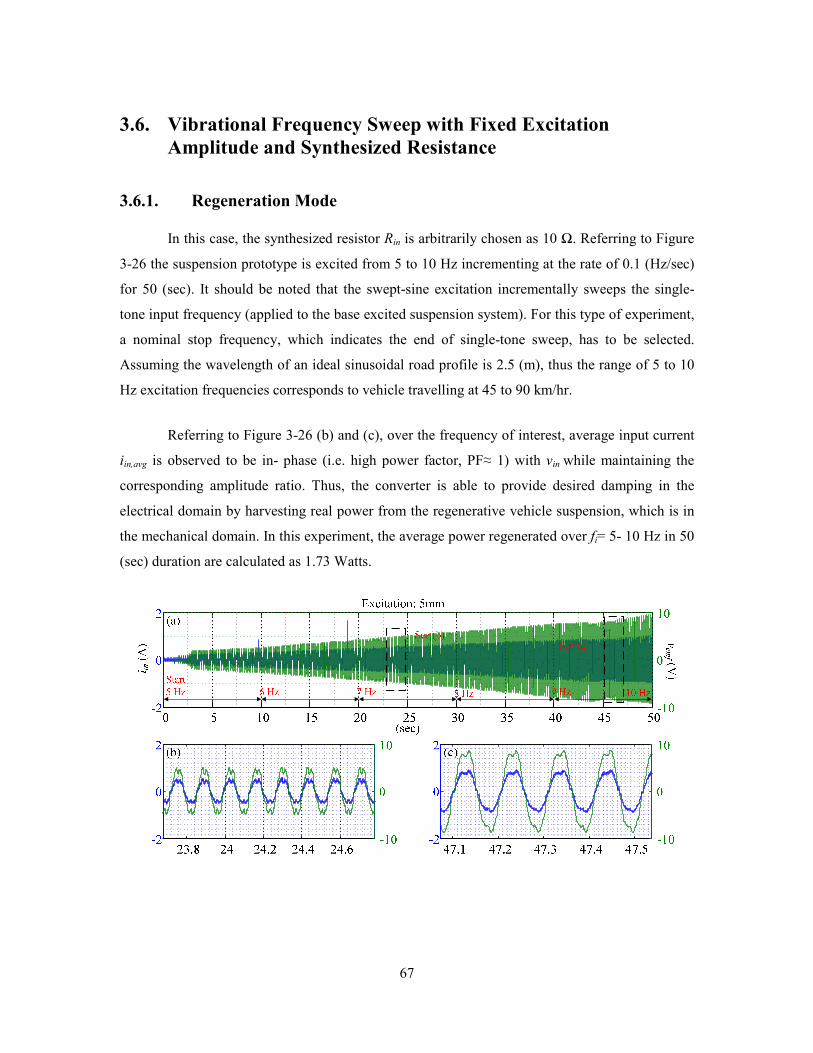
67
3.6. Vibrational Frequency Sweep with Fixed Excitation
Amplitude and Synthesized Resistance
3.6.1. Regeneration Mode
In this case, the synthesized resistor Rin is arbitrarily chosen as 10 Ω. Referring to Figure
3-26 the suspension prototype is excited from 5 to 10 Hz incrementing at the rate of 0.1 (Hz/sec)
for 50 (sec). It should be noted that the swept-sine excitation incrementally sweeps the single-
tone input frequency (applied to the base excited suspension system). For this type of experiment,
a nominal stop frequency, which indicates the end of single-tone sweep, has to be selected.
Assuming the wavelength of an ideal sinusoidal road profile is 2.5 (m), thus the range of 5 to 10
Hz excitation frequencies corresponds to vehicle travelling at 45 to 90 km/hr.
Referring to Figure 3-26 (b) and (c), over the frequency of interest, average input current
iin,avg is observed to be in- phase (i.e. high power factor, PF≈ 1) with vin while maintaining the
corresponding amplitude ratio. Thus, the converter is able to provide desired damping in the
electrical domain by harvesting real power from the regenerative vehicle suspension, which is in
the mechanical domain. In this experiment, the average power regenerated over fi= 5- 10 Hz in 50
(sec) duration are calculated as 1.73 Watts.

68
Figure 3-26: (a) Motor back EMF and current waveforms synthesizing Rin= 10 Ω by sweeping
excitation frequencies from 5 to 10 Hz in 50 seconds (i.e. 0.1 Hz/ sec) with 5mm excitation
amplitude. (b) Detailed instantaneous waveform indicating Rin= 10 Ω at vibration frequency ≈ 7.4
Hz and (c) ≈ 9.7 Hz.
3.6.2. Motoring Mode
While the SMR is operating in motoring mode, it synthesizes negative resistor (Rin< 0 Ω).
Again, operations in motoring mode require draining of battery energy. This corresponds to the
generation of negative damping in the electrical domain of the suspension system. In this case, Rin
is arbitrarily chosen as -100 Ω. Referring to Figure 3-27 (a) to (c), over the frequency of interest,
the average input current iin,avg is observed to be out of phase (i.e. PF≈ -1) with vin while
maintaining the corresponding amplitude ratio. In addition, to observe battery drainage, the
battery current iDC is also depicted along with EMF voltage vemf and converter current iin. As seen
in Figure 3-28 (a) at roughly 2.5 (sec), the base initiates ground vibration at approximately 2.5
(Hz) and 5mm, the converter current is controlled to suffice Rin= -100 Ω with respect to EMF
voltage. At this time, the negative battery current clearly starts, which indicates drainage.
Figure 3-27: (a) Motor back EMF and current waveforms synthesizing Rin= -100 Ω by sweeping
excitation frequencies from 5 to 10 Hz in 50 seconds (i.e. 0.1 Hz/ sec) with 5mm excitation
amplitude. (b) Detailed instantaneous waveform indicating Rin= -100 Ω at vibration frequencies ≈
7 Hz and (c) ≈ 9 Hz.

69
Figure 3-28: (a) Transients of Motor back EMF and current waveforms synthesizing Rin= -100 Ω.
(b) Negative battery current indicating converter is placed in motoring mode.
3.6.3. Mechatronic System Conversion Efficiency
The power flow of the proposed mechatronic system is displayed in Figure 3-29. The
analysis can be divided into mechanical (i.e. road excitation/ suspension system) and electrical
domains (i.e. AC/DC converters/ battery packs). The overall efficiency of power regeneration η is
defined in (3-17) as the product of mechanical effiency ηm, generator efficiency ηe, and AC/DC
rectifier efficiency ηAC/DC
/m e AC DCη η η η= (3-17)
where ηme is the overall efficiency of the electro- magnetic suspension. The instantaneous power,
provided by road force, supplies to the system (Pall) is equal to the sum of instantaneous power
dissipated by physical friction (Pf), absorbed by the DC machine (Pc), and required to build up
sprung-mass oscillation (Pk). This means that, only the power absorbed by the electrical damping
contributes to the power regeneration; therefore, the mechanical efficiency can be defined as

70
c cm
all c f k
P P
P P P Pη = =
+ +
(3-18)
The instantaneous available power provided by the DC machine represents the total power
transferred to the electrical domain is defined as
( ) 12
intc in loadP v R R−
= + . (3-19)
The instantaneous harvestable power, which represents the power transferred to the attached
power converter, can be written as
( ) 1
inte c load loadP P R R R−
= + . (3-20)
The electrical efficiency ηe degradation by the motor winding and other losses in the AC/DC
converter can be derived as
( ) 1
inte load loadR R Rη −≈ + .
(3-21)
cP
fP
kP
allPeP
lP /e all m e AC DCP P η η η=
Figure 3-29: Mechatronic systems power flow.

71
Figure 3-30: Theoretical electrical efficiency ηe and generated (harvestable) power Pe with
various DC motor internal resistors Rint and synthesized resistors Rin assuming EMF voltage
equals to 10 sin(10πt). Note: The plot only depicted maximum Rin= 30 Ω
Figure 3-31: Instantaneous (a) SMR power conversion efficiency ηAC/DC and (b) electrical domain
efficiency ηe over the swept frequencies synthesizing Rin= 10 Ω.
Referring to Figure 3-30, the nominal Pe and ηe are calculated for every value of Rint and Rin.
Different Rint represents power dissipated by different types of DC brushed machine. As
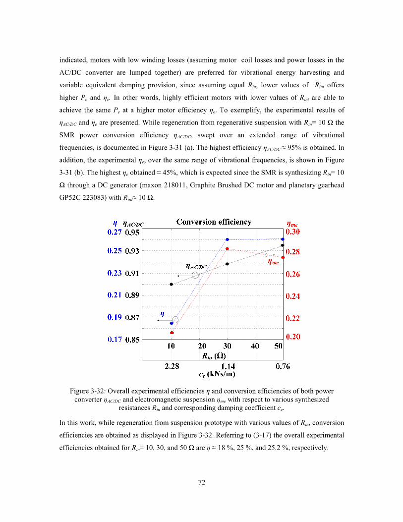
72
indicated, motors with low winding losses (assuming motor coil losses and power losses in the
AC/DC converter are lumped together) are preferred for vibrational energy harvesting and
variable equivalent damping provision, since assuming equal Rin, lower values of Rint offers
higher Pe and ηe. In other words, highly efficient motors with lower values of Rint are able to
achieve the same Pe at a higher motor efficiency ηe. To exemplify, the experimental results of
ηAC/DC and ηe are presented. While regeneration from regenerative suspension with Rin= 10 Ω the
SMR power conversion efficiency ηAC/DC, swept over an extended range of vibrational
frequencies, is documented in Figure 3-31 (a). The highest efficiency ηAC/DC ≈ 95% is obtained. In
addition, the experimental ηe, over the same range of vibrational frequencies, is shown in Figure
3-31 (b). The highest ηe obtained ≈ 45%, which is expected since the SMR is synthesizing Rin= 10
Ω through a DC generator (maxon 218011, Graphite Brushed DC motor and planetary gearhead
GP52C 223083) with Rint≈ 10 Ω.
Figure 3-32: Overall experimental efficiencies η and conversion efficiencies of both power
converter ηAC/DC and electromagnetic suspension ηme with respect to various synthesized
resistances Rin and corresponding damping coefficient ce.
In this work, while regeneration from suspension prototype with various values of Rin, conversion
efficiencies are obtained as displayed in Figure 3-32. Referring to (3-17) the overall experimental
efficiencies obtained for Rin= 10, 30, and 50 Ω are η ≈ 18 %, 25 %, and 25.2 %, respectively.

73
3.7. Experimental Variable Resistor Synthesis under ISO
Standard Excitations
To verify the performance of SMR while placed under ISO road profiles the suspension
prototype is exited according to the generated ISO class C and D road profiles as shown in Figure
3-33. As expected, since higher road classes indicate higher PSD, the excitation amplitude across
a nominal time range (i.e. 30 seconds) is higher. In order to enlarge the region of resistance
synthesis the SMR is swept from minimum to maximum resistances of 10 Ω (damping coefficient
ce= 2.28 kNs/m) to 100 Ω (ce= 0.41 kNs/m) in 30 (sec) using ISO standard road profile (class C)
as shown in Figure 3-34 (a). The detailed instantaneous waveforms of vx and iin depicted in Figure
3-34 (b) to (e) demonstrate high power factor with the variations of desired Rin through
corresponding amplitude ratios. For detailed instantaneous performance of the SMR, a video was
posted to demonstrate the experimental sweep of the resistor synthesis on dSPACE ControlDesk
[85]. Similarly, the resistance sweep is also performed for class D road class as shown in Figure
3-35. Compared to class C the EMF voltage is higher due to larger excitation amplitude (and
higher frequency components), which leads to higher converter current (for the same value of
synthesized resistor).
Figure 3-33: ISO 8608 class C (blue) and D (red) excitation profile travelling at 25 km/hr.

74
Figure 3-34: (a) Variable resistance sweep from 10 to 100 Ω. (b) Detailed corresponding line
current iin and voltage vemf for synthesizing Rin= 10 Ω, (c) Rin= 30 Ω, (d) Rin= 50 Ω, and (e) Rin=
100Ω with class C road roughness and vehicle speed = 25 km/hr.

75
Figure 3-35(a) Variable resistance sweep from 10 to 100 Ω. Detailed corresponding line current
iin and voltage vemf for synthesizing (b) Rin= 10 Ω, (c) Rin = 50 Ω, (d) Rin = 100 Ω with class D
road roughness and vehicle speed = 25 km/hr.
By referring to Figure 3-36 the detailed inverter voltage vc and rectified current iDC with respect to
EMF voltage and reference converter current is observed. In this case, a nominal Rin= 20 Ω is
synthesized. As indicated in both Figure 3-9 and Figure 3-16, the switching modes vary from
Mode 1- 3 depending on the location of error current ierr within the pre-defined error- band.
Figure 3-36: (a) Back EMF, (b) converter current for synthesizing Rin= 20 Ω, (c) controlled
inverter voltage, and (d) harvested current with class D road roughness at vehicle speed = 50
km/hr.
In addition, the SMR also operates in bi- directional power flow. This can be verified by
observing inverter voltage vDC, vemf, iin, and rectified current iDC in Figure 3-37. In this work, the
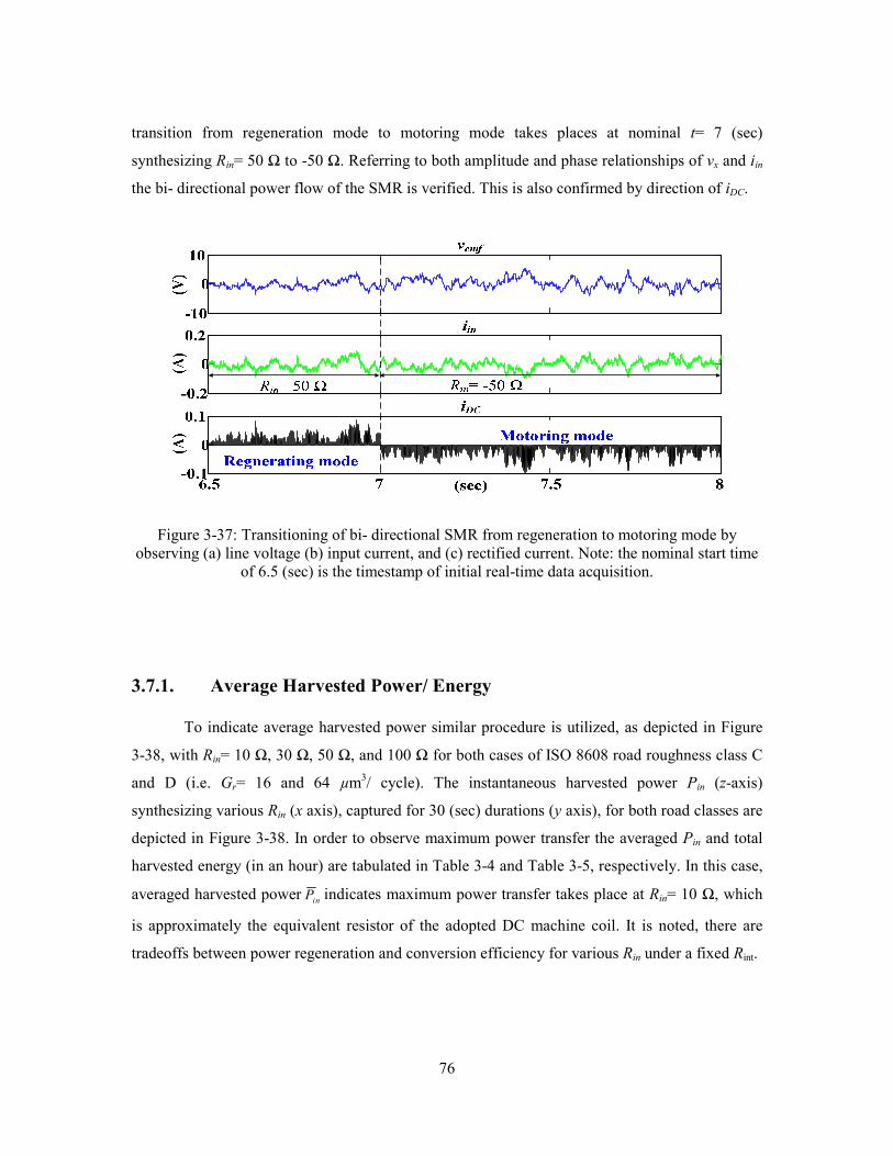
76
transition from regeneration mode to motoring mode takes places at nominal t= 7 (sec)
synthesizing Rin= 50 Ω to -50 Ω. Referring to both amplitude and phase relationships of vx and iin
the bi- directional power flow of the SMR is verified. This is also confirmed by direction of iDC.
Figure 3-37: Transitioning of bi- directional SMR from regeneration to motoring mode by
observing (a) line voltage (b) input current, and (c) rectified current. Note: the nominal start time
of 6.5 (sec) is the timestamp of initial real-time data acquisition.
3.7.1. Average Harvested Power/ Energy
To indicate average harvested power similar procedure is utilized, as depicted in Figure
3-38, with Rin= 10 Ω, 30 Ω, 50 Ω, and 100 Ω for both cases of ISO 8608 road roughness class C
and D (i.e. Gr= 16 and 64 µm3/ cycle). The instantaneous harvested power Pin (z-axis)
synthesizing various Rin (x axis), captured for 30 (sec) durations (y axis), for both road classes are
depicted in Figure 3-38. In order to observe maximum power transfer the averaged Pin and total
harvested energy (in an hour) are tabulated in Table 3-4 and Table 3-5, respectively. In this case,
averaged harvested powerinP indicates maximum power transfer takes place at Rin= 10 Ω, which
is approximately the equivalent resistor of the adopted DC machine coil. It is noted, there are
tradeoffs between power regeneration and conversion efficiency for various Rin under a fixed Rint.
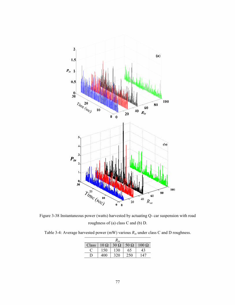
77
Figure 3-38 Instantaneous power (watts) harvested by actuating Q- car suspension with road
roughness of (a) class C and (b) D.
Table 3-4: Average harvested power (mW) various Rin under class C and D roughness.
Rin
Class 10 Ω 30 Ω 50 Ω 100 Ω
C 150 130 65 43
D 400 320 250 147

78
Table 3-5: Total estimated energy harvested (in Watt- hour) with Rin = 10 and 50 Ω under ISO
class C and D roughness.
Rin
Class 10 Ω 50 Ω
C 18 5.1
D 48 30
3.8. Regenerative Semi-Active Control using SMR
In this work, we proposed a mechatronic suspension system with capabilities of energy
regeneration and sky-hook (SK) control incorporated into the mechanism [100]. The system
overcomes the tradeoffs between energy consumption and ride handling/comfort in an active
(semi-active) suspension system. Central to the concept is development of a coupled switched-
mode rectifier (SMR) capable of providing either a positive or negative damping ratio by
alternating between regenerative and motoring modes. Using the implemented circuit, an active
sky-hook control strategy is utilized to offer continuous variable damping force that improves the
vibration isolation significantly. Simulation results demonstrated the directions of power flow in
both regeneration and motoring modes, through a current controller, to verify performance of the
SMR. Experimental results demonstrated both time and frequency response of the regenerative
suspension prototype in terms of power regeneration, sprung mass absolute acceleration, and
relative displacement. In addition, both theoretical and experimental power conversion
efficiencies in various segments of the mechatronic suspension are analyzed and reported.
To this end, various works have proposed semi-active control scheme that can maintain
the reliability of passive control using an acceptable amount of energy [101]- [107]. Semi-active
control strategies utilizing innovative magnetorheological (MR) fluid damper designs have been
proposed by several researchers (see e.g. [101]- [107]). In addition, the R-S control method
implemented to minimize the damping force when the spring force and damping force have the
same direction is proposed in [108]. The experimental results of three semi-active control
methods, (i.e. limited relative displacement, modified R-S, and modified sky-hook) verified in
terms of tradeoffs between vehicle handling and passenger comfort, are reported in [109].
Although the “on-off” semi-active methods are efficient in suspension control, they result in
uncomfortable jumps when switching between on and off modes. Hence, there would be a

79
sacrifice in the control performance when compared with the continuously variable type. In
[110]- [111], a modified Skyhook fuzzy controller in the design of a semi-active suspension
system for a Cadillac SRX 2005 is demonstrated with road tests results. Their real-time
experiments confirmed that the use of this design method reduces the required time and effort in
real industrial problems.
In addition to various approaches of suspension control, power regeneration from vehicle
suspension, through an electromagnetic device, has become extremely popular (e.g. [112]-[114]).
The common drawbacks of the mechatronic systems discussed previously is the consumption of
electrical power (DC current required for MR damper) while generating corresponding forces for
purposes of better handling/ comfort. For example, the approach taken in semi- active control
implementation in [109] supplied various level of DC current to the MR damper for achieving
variable levels of damping forces. On the contrary, the proposed method is capable of selectively
apply variable damping forces while regenerate the damped power according to the adopted semi-
active control algorithm.
The damping force, with respect to relative velocity zɺ, for a 1-DOF system with a
Skyhook damper can be written as
sky skyF c z= ɺ . (3-22)
Using a semi-active damper, the Skyhook damping force must be realized in terms of the relative
velocityzɺ. Therefore, the conventional semi-active Skyhook control algorithm is given by [109]-
[110]
0
0 0
sky
sky
c z xzF
xz
≥=
<
ɺɺ ɺ
ɺɺ (3-23)
where the presence (on)/ absence (off) of damping force Fsky is required according to the signed
product of relative and absolute velocity. As for the proposed active Skyhook control strategy, the
damper can supply a negative force from a negative damping ratio− . In this case, the active
Skyhook control algorithm can be written as

80
0
0
sky
sky
sky
c z xzF
c z xz
≥= − <
ɺɺ ɺ
ɺɺ ɺ. (3-24)
Recalling (3-24), in order to implement the control algorithm in the electrical- domain, by the
SMR, the converter current should be controlled to the following reference current
( )( ) 1 1
int 0ref e g loadi k k R R d z xz− −= + ≥ɺɺ ɺ (3-25)
( )( ) 1 1
int 0ref e g loadi k k R R d z xz− −= − + <ɺɺ ɺ . (3-26)
0 0ref
i xz= <ɺɺ . (3-27)
When 0xz <ɺɺ , iref is determined by (3-26)- (3-27) for either better vehicle control or power
harvesting, respectively. This is due to negative direction of current results in power consumption
of the load batteries, by recalling section 3.2. The detailed analysis of the current controller is
presented in the following sections.
3.8.1. Simulation Results
The simulation of the regenerative suspension system, connected to SMR, is performed in
MATLAB/SIMULINK/Simscape/SymPowerSystem environment. The values of the main
parameters for the quarter-car suspension prototype and DC motor (based on maxon 218011,
Graphite Brushed DC motor and planetary gearhead GP52C 223083) are the following. m= 5.4
kg, ma= 0.257 kg, k= 7.3 kN/m, cf= 100 N- sec/ m, ke=kt= 0.1 (V- sec/rad, N- m/A), kg= 10, Jm=
101e-7
kg- m2, Ja= 1.2e
-4 kg- m
2 Jg= 9.1e
-7 kg- m
2, d=l/2π= 0.0095 mm/rev (based on THK ball-
screw KX-10), Rs= 10Ω, and Ls= 2.62mH. The values of SMR and DB- HCC are Ra= 1mΩ, La=
1mH, VDC = 20 V, small error- band = 0.2 A, and large error- band = 0.3 A.

81
The simulated waveforms, in Figure 3-39 (a), indicate the behavior of line (EMF) voltage
vin, iin and iref assuming the regenerative suspension is under single-tone harmonic excitation.
According to the sky-hook detection outcome, shown in Figure 3-39 (c), SMR presents positive
or negative damping according to the polarity of sign(viniin). Moreover, as observed, iin is
regulated within the error-band to iref , which is determined by vin and its polarity varies with
respect to the sky-hook detection outcome. Figure 3-39 (b) indicates more detailed current
waveforms of iin and iref. It is observed that before entering the motoring mode, the small-band
state loses regulation and returns to the large-band state. Once entered in the motoring mode (i.e.
sign(viniin)< 0), both waveforms are out-of-phase with vin. On the contrary, when placed in the
regeneration mode, both waveforms are in-phase with vin.
Figure 3-39: (a) Line (EMF) voltage vin, current iin, and reference current iref. (b) Detailed
depiction of iin and iref indicating motoring and regeneration modes operation, by (c) Sky- hook
detection outcome.
To verify the DB-HCC control law state diagram, Figure 3-40 (a) simulates the behavior of it and
rectified current, which stores energy into the battery. The detailed switching waveforms are
shown in Figure 3-40 (b), where the SMR enters the motoring mode from regeneration mode. In
this case while operating in regeneration mode, both sign(vin)> 0 and sign(viniin)> 0, therefore,
SMR alternates between Mode 1 and 2 as shown previously in Figure 3-9. After entering the
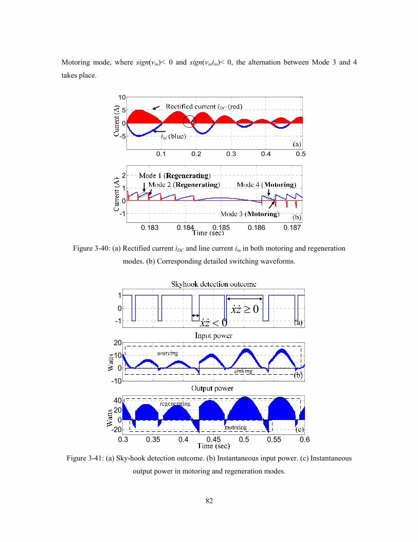
82
Motoring mode, where sign(vin)< 0 and sign(viniin)< 0, the alternation between Mode 3 and 4
takes place.
0.1 0.2 0.3 0.4 0.5
-5
0
5
10
0.183 0.184 0.185 0.186 0.187
-1
0
1
2
Figure 3-40: (a) Rectified current iDC and line current iin in both motoring and regeneration
modes. (b) Corresponding detailed switching waveforms.
0.3 0.35 0.4 0.45 0.5 0.55 0.6
-1
0
1
0.3 0.35 0.4 0.45 0.5 0.55 0.6-10
0
10
20
0.3 0.35 0.4 0.45 0.5 0.55 0.6
-20
0
20
40
0xz ≥ɺɺ0xz <ɺɺ
Figure 3-41: (a) Sky-hook detection outcome. (b) Instantaneous input power. (c) Instantaneous
output power in motoring and regeneration modes.

83
According to the sky-hook detection outcome in Figure 3-41 (a), both input and output power
shown in Figure 3-41 (b) and Figure 3-41 (c), respectively, indicate regeneration and motoring
modes taking place according to their instantaneous polarities. Again, synthesizing negative
damping, implies transferring negative source power. Therefore, in the motoring mode the power
is transferred from battery to source. Thus, energy harvesting is achieved in regeneration mode,
while the stored energy is used to supply the power required in the motoring mode.
3.8.2. Experimental Skyhook Detection
According to the experimental configuration of the mechatronic system, shown in Figure
3-42, the converter prototype is coupled to the 1-DOF base excited regenerative suspension
system fabricated by Intelligent Vehicles Lab at Simon Fraser University. As depicted, the source
and load of a bi- directional SMR, controlled by double band hysteresis current control (DB-
HCC), is coupled to terminals of DC generator/ motor, Graphite Brushed DC motor and planetary
gearhead and a rechargeable battery. As previously described in (3-23)- (3-25), since the SK
control method requires either presence or absence of damping forces according to the product of
absolute and relative sprung mass velocity. Identically, to realize such performance in the
electrical domain the connected power converter is required to present constant Rin, -Rin or “open
circuit” (i.e. iref = 0 A) to the motor terminal. In this work, to maximize power regeneration, the
SMR is we designated to only remain in regeneration mode. Meaning, the reference current iref,
derived from motor EMF vemf, switches between iref = 0 A and iref= vemf /(Rint+Rin). When 0xz <ɺɺ
(i.e. iref = 0 A) the power generated by DC generator/ motor is equivalently disconnected to the
electrical domain. When 0xz ≥ɺɺ (i.e. iref = vemf /(Rint+Rin), since the SMR synthesizes a variable
resistor, real power generated by the DC generator/ motor is then harvested into a load battery.
To verify the efficacy of the regenerative Skyhook algorithm, the electromagnetic
suspension, shown in Figure 3-43 (a), is placed under swept sine excitation, by a MTS 248
hydraulic actuator, over an extended range of vibrational frequencies. In this work, the suspension
is excited from 2- 9 Hz by fixed amplitude of 5mm at the rate of 0.2 (Hz/ sec) for 35 (sec), as
depicted in Figure 3-43 (a). The resulting harvested power, sprung mass absolute velocity, and
relative velocity for Rin= 10 Ω are demonstrated in Figure 3-43 (b) and (c), respectively.
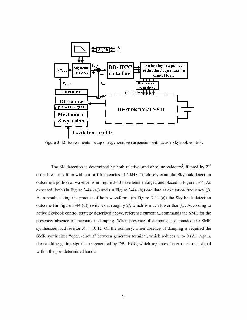
84
Figure 3-42: Experimental setup of regenerative suspension with active Skyhook control.
The SK detection is determined by both relative zɺ and absolute velocityxɺ, filtered by 2nd
order low- pass filter with cut- off frequencies of 2 kHz. To closely exam the Skyhook detection
outcome a portion of waveforms in Figure 3-43 have been enlarged and placed in Figure 3-44. As
expected, both (in Figure 3-44 (a)) and (in Figure 3-44 (b)) oscillate at excitation frequency (f).
As a result, taking the product of both waveforms (in Figure 3-44 (c)) the Sky-hook detection
outcome (in Figure 3-44 (d)) switches at roughly 2f, which is much lower than fsw. According to
active Skyhook control strategy described above, reference current iref commands the SMR for the
presence/ absence of mechanical damping. When presence of damping is demanded the SMR
synthesizes load resistor Rin = 10 Ω. On the contrary, when absence of damping is required the
SMR synthesizes “open -circuit” between generator terminal, which reduces iin to 0 (A). Again,
the resulting gating signals are generated by DB- HCC, which regulates the error current signal
within the pre- determined bands.

85
Figure 3-43: (a) Swept- sine excitation profile from 2- 9 Hz ( at 0.2 Hz/ sec) in 35 (sec) with Y=
5mm. (b) Instantaneous harvested power, (c) absolute velocity, and relative velocity as a result of
active SK with Rin= 10 Ω synthesis. Note: Signals inside the dashed boxes are enlarged in the
next figure.
0xz ≥ɺɺ
Figure 3-44: (a) Detailed absolute velocity, (b) relative velocity, (c) the corresponding product,
and (d) its’ SK detection outcome at f ≈ 7 Hz.
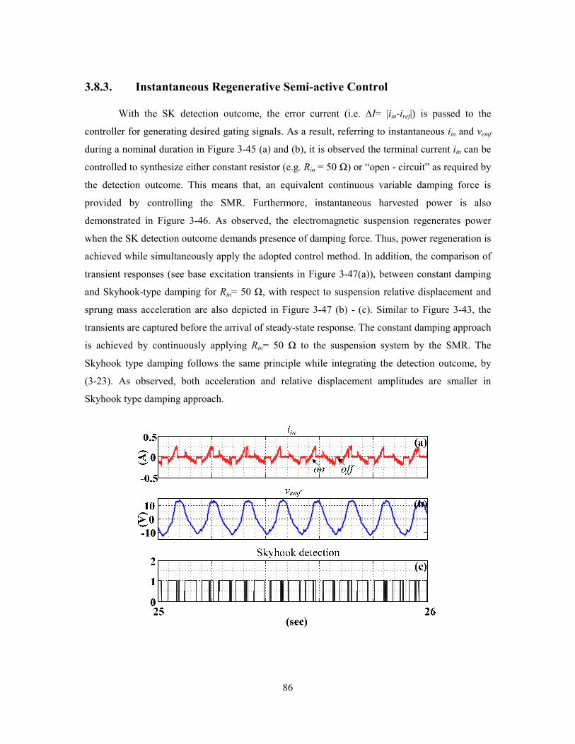
86
3.8.3. Instantaneous Regenerative Semi-active Control
With the SK detection outcome, the error current (i.e. ∆I= |iin-iref|) is passed to the
controller for generating desired gating signals. As a result, referring to instantaneous iin and vemf
during a nominal duration in Figure 3-45 (a) and (b), it is observed the terminal current iin can be
controlled to synthesize either constant resistor (e.g. Rin = 50 Ω) or “open - circuit” as required by
the detection outcome. This means that, an equivalent continuous variable damping force is
provided by controlling the SMR. Furthermore, instantaneous harvested power is also
demonstrated in Figure 3-46. As observed, the electromagnetic suspension regenerates power
when the SK detection outcome demands presence of damping force. Thus, power regeneration is
achieved while simultaneously apply the adopted control method. In addition, the comparison of
transient responses (see base excitation transients in Figure 3-47(a)), between constant damping
and Skyhook-type damping for Rin= 50 Ω, with respect to suspension relative displacement and
sprung mass acceleration are also depicted in Figure 3-47 (b) - (c). Similar to Figure 3-43, the
transients are captured before the arrival of steady-state response. The constant damping approach
is achieved by continuously applying Rin= 50 Ω to the suspension system by the SMR. The
Skyhook type damping follows the same principle while integrating the detection outcome, by
(3-23). As observed, both acceleration and relative displacement amplitudes are smaller in
Skyhook type damping approach.

87
Figure 3-45: (a) Converter current iin (b) and EMF voltage for Rin= 50 Ω synthesis according to
SK detection outcome at f≈ 7 Hz. Note: Examples of presence and absence of damping are
indicated by “on” and “off”.
Figure 3-46: Instantaneous harvested power for Rin= 50 Ω synthesis according to SK detection
outcome.
Figure 3-47: (a) Transients of base excitation profile. Comparison of (b) absolute acceleration and
(c) relative displacement transients between synthesized Skyhook control and constant damping.

88
3.8.4. Experimental Frequency Response with Regenerative Automotive
Suspension
To assess suspension dynamic performance in terms of vehicle handling and passenger
comfort and harvested power, various values of Rin are chosen for active SK control. Again, the
electromagnetic suspension is excited by profiles shown in Figure 3-43 (a). The results obtained
by SMR synthesizing Rin= 10, 50, 100 Ω are presented as well as Rin= ∞ and 0 Ω for minimum
and maximum equivalent damping are included for comparisons. In this work, Rin= ∞ and 0 Ω are
realized by opening and shorting the motor terminals during the entire experiment, therefore, no
power harvesting can take place.
( ) 1 2e
s
f
rms e s
f
f f dfλ λ−= − ∫ (3-28)
( ) 1 2e
s
f
rms e s
f
f f dfη η−= − ∫ (3-29)
( ) 1e
s
f
L e s L
f
P f f P df−
= − ∫ (3-30)
As indicated in (3-28) and (3-29), the vehicle handling (or suspension workspace limit)
and passenger comfort are measured by the RMS of suspension relative displacement
transmissibility ηrms and sprung mass acceleration λrms over the excited spectrum (i.e. f= fs to fe),
respectively. In addition, according to (3-30), the average harvested power PL is also assed for
maximum power charging. Referring to frequency responses in Figure 3-48 and normalized RMS
values tabulated in Table 3-6 it is realized Rin = 0 Ω offers the best vehicle handling with worst
passenger comfort while Rin = ∞ Ω indicates the opposite outcome; when coupling SMR to the
regenerative suspension prototype Rin = 100 Ω delivers the best overall handling/ comfort while
Rin = 10 Ω scavenges the maximum amount of vibrational power.

89
(a) (b)
(c)
Figure 3-48: Frequency response of absolute acceleration λ (c) relative displacement
transmissibility η and (d) harvested power PL of regenerative Skyhook control algorithm for
various values of synthesized Rin
Table 3-6 Normalized RMS of acceleration and relative displacement and average harvested
power obtained with different values of Rin
Rin (Ω) ηrms/ ηmax λrms/ λ max LP / PL, max
0 0.24 1 n/a
10 0.47 0.90 1
50 0.79 0.68 0.39
100 0.86 0.63 0.25
∞ 1 0.59 n/a

90
3.9. Chapter Summary
In this chapter, the concept of using a bi-directional switched-mode rectifier (SMR) for
synthesizing variable electrical damping is demonstrated in both simulations and experimental
environments. To exemplify energy harvesting capabilities, the SMR is placed under both swept-
sine and ISO standard road profiles for demonstrating the current controller regulating the SMR
current according to both sinusoidal and stochastic DC machine EMF, respectively. It is noted,
the hysteresis current controller is able to accurately synthesize desired resistors (i.e. regulating
converter current) according to line voltage (both amplitudes and frequencies) that is unknown a-
priori. In addition, the integration of semi- active control and energy harvesting is denoted. It is
demonstrated, through both time and frequency responses, double- band hysteresis current
controller (DB- HCC) is able to selectively synthesize positive (i.e. regenerating mode), negative
(i.e. motoring mode), or zero (i.e. equvilent open circuit) equivalent dampings according to the
Skyhook detection outcome, which shows that the SMR, controlled by HCC, can indeed attain
suspension semi- active control and road energy harvesting simulatanoeusly.
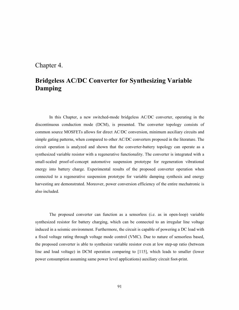
91
Chapter 4.
Bridgeless AC/DC Converter for Synthesizing Variable
Damping
In this Chapter, a new switched-mode bridgeless AC/DC converter, operating in the
discontinuous conduction mode (DCM), is presented. The converter topology consists of
common source MOSFETs allows for direct AC/DC conversion, minimum auxiliary circuits and
simple gating patterns, when compared to other AC/DC converters proposed in the literature. The
circuit operation is analyzed and shown that the converter-battery topology can operate as a
synthesized variable resistor with a regenerative functionality. The converter is integrated with a
small-scaled proof-of-concept automotive suspension prototype for regeneration vibrational
energy into battery charge. Experimental results of the proposed converter operation when
connected to a regenerative suspension prototype for variable damping synthesis and energy
harvesting are demonstrated. Moreover, power conversion efficiency of the entire mechatronic is
also included.
The proposed converter can function as a sensorless (i.e. as in open-loop) variable
synthesized resistor for battery charging, which can be connected to an irregular line voltage
induced in a seismic environment. Furthermore, the circuit is capable of powering a DC load with
a fixed voltage rating through voltage mode control (VMC). Due to nature of sensorless based,
the proposed converter is able to synthesize variable resistor even at low step-up ratio (between
line and load voltage) in DCM operation comparing to [115], which leads to smaller (lower
power consumption assuming same power level applications) auxiliary circuit foot-print.
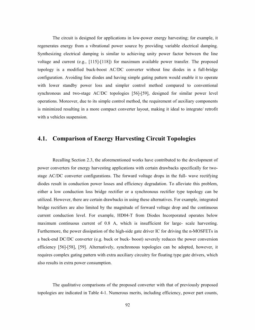
92
The circuit is designed for applications in low-power energy harvesting; for example, it
regenerates energy from a vibrational power source by providing variable electrical damping.
Synthesizing electrical damping is similar to achieving unity power factor between the line
voltage and current (e.g., [115]-[118]) for maximum available power transfer. The proposed
topology is a modified buck-boost AC/DC converter without line diodes in a full-bridge
configuration. Avoiding line diodes and having simple gating pattern would enable it to operate
with lower standby power loss and simpler control method compared to conventional
synchronous and two-stage AC/DC topologies [56]-[59], designed for similar power level
operations. Moreover, due to its simple control method, the requirement of auxiliary components
is minimized resulting in a more compact converter layout, making it ideal to integrate/ retrofit
with a vehicles suspension.
4.1. Comparison of Energy Harvesting Circuit Topologies
Recalling Section 2.3, the aforementioned works have contributed to the development of
power converters for energy harvesting applications with certain drawbacks specifically for two-
stage AC/DC converter configurations. The forward voltage drops in the full- wave rectifying
diodes result in conduction power losses and efficiency degradation. To alleviate this problem,
either a low conduction loss bridge rectifier or a synchronous rectifier type topology can be
utilized. However, there are certain drawbacks in using these alternatives. For example, integrated
bridge rectifiers are also limited by the magnitude of forward voltage drop and the continuous
current conduction level. For example, HD04-T from Diodes Incorporated operates below
maximum continuous current of 0.8 A, which is insufficient for large- scale harvesting.
Furthermore, the power dissipation of the high-side gate driver IC for driving the n-MOSFETs in
a back-end DC/DC converter (e.g. buck or buck- boost) severely reduces the power conversion
efficiency [56]-[58], [59]. Alternatively, synchronous topologies can be adopted, however, it
requires complex gating pattern with extra auxiliary circuitry for floating type gate drivers, which
also results in extra power consumption.
The qualitative comparisons of the proposed converter with that of previously proposed
topologies are indicated in Table 4-1. Numerous merits, including efficiency, power part counts,

93
gate drives design, sensed signals, are tabulated. The two- stage topologies, implemented for
pizeo-based application [56]-[58], [59], generally bears low efficiency due to its low available
power level and rectification conduction loss in the AC/DC segment. The two-switch
synchronous boost topologies [72] appeared with the lowest part counts and conduction loss due
to absence of rectifying diode. The conversion efficiency is claimed in the vicinities of 92%,
however, the power consumption and design of gate driver was not documented. A direct AC/DC
topologies implemented in [74] possess high part count due to additional load battery with similar
conduction loss to the proposed topology in this work. However, the switching modes and
analysis of the converter operation were not clearly illustrated. Instead, the application of the
converter, which is applying damping in a tuned- mass-spring- damper environment, is carried
out experimentally.
Table 4-1: Energy harvesting topologies comparisons
Converter Type Conversion
efficiency
Converter
part counts
Driver
design
Operation
modes
Sensed
signals
Two-stage [56]-[58], [59]
(piezoelectric) < 50% High High side DCM
Sensor-
less
Synchronous boost
rectifier [73]
(electromagnetic)
≈ 92% Low n/a DCM Line
voltage
Direct AC/DC [74]
(electromagnetic) n/a High n/a DCM n/a
Switch- mode rectifier
(electromagnetic) 90- 93.5% Low
High and
low side CCM
Line
current
Proposed topology
(electromagnetic) 87- 94% Medium Low side DCM
Sensor-
less
Similar to SMR, the proposed direct rectification topology also provides variable damping
(positive) to the connected dynamic system. In addition, it provides flexibility in gate drive
design, according to available power level of the seismic source, which the conventional SMR
topology does not offer. Moreover, the proposed topology allows simpler transition between
different switch- modes when connected to more realistic irregular voltage source. On the
contrary, SMR provides bi- directional power flow, meaning it is able to provide bipolar electrical
damping, while the proposed direct AC/DC converter is only capable of supplying positive

94
electrical damping. To illustrate the operation and benefit of the proposed converter the
comparisons, in terms of the various operating modes and input power, between direct AC/DC
and synchronous boost rectifier [72] are demonstrated.
4.2. Proposed Bridgeless Converter Topology
The proposed converter is shown in Figure 4-1 (a), which is a single stage direct AC/DC
buck-boost converter operating in DCM. The configuration is inspired by battery charging
circuits, where back-to-back MOSFETs are utilized for over-charge and over-discharge
protection [119]-[120]. In this converter, the common source configuration provides bi-
directional current conduction and blocking capabilities. The configuration is utilized to ensure
line voltage vin is disconnected from inductor L during its discharging period in the entire line
cycle. The back-to-back configuration is placed intentionally to prevent undesired conduction via
the undesired path. For example, if SWMOS only consisted of a single MOSFET with its drain
connected to vin, during negative line cycle, even if SWMOS is turned off, the body diode will still
be forward biased if vin is higher than body diode forward voltage VF.
ini
MOSSW
pQ
oVL
inv
nQ
1C 2C
oiFV
1Cv 2Cv
Lv
Li
pQi
nQi
2Ci
1Ci
(a)

95
L
2SW1SW
1D 2D
inv
(b)
1SW
2SW
(c)
Figure 4-1: (a) Proposed bi- directional bridgeless AC/DC converter. (b) Two- switch type
synchronous rectifier and (c) its’ gating pattern for DCM operation.
Compared to a synchronous boost converter operating in DCM, in Figure 4-1 (b), the main
advantages are as follows [72]. The conduction loss in power stage is the primary contributor of
power efficiency degradation in DCM operation. Thus the proposed converter avoids additional
conduction losses contributed by RDS,on of either SW1 or SW2 in synchronous boost converter (see
Figure 4-1(b)) during the inductor discharging period. Moreover, the synthesized input resistance
by the proposed converter is a function of time-independent variables (shown later). In addition,
the gating pattern of the proposed topology is extremely straightforward, where both n-MOSFETs
are gated simultaneously. On the contrary, either SW1 or SW2 is required to switch on for the
entire half line cycle, which leads to more a complex gating pattern with line polarity detection
(see Figure 4-1(c)) needed to realize such operation. In addition, the gate drive output is required
to remain logic high in order for SW2 to form a closed-loop system. Therefore, during the
charging of L, the power dissipation/conduction losses are higher due to RDS,ON of SW2. The gating
pattern also leads to unequalled duty cycles and stress between both n-MOSFETs and potentially
limits choosing the modulation carrier frequency and MOSFET’s safe operating area (SOA).

96
4.3. Converter Analysis and Modelling
In this section, the switching waveforms of the proposed converter are assumed to be ideal,
including MOSFET switching dynamics, zero forward voltage drops across the diodes, and zero
series resistances for passive elements. Note that other than opposite current flow, in order to
facilitate simple gating pattern, the operation of the proposed topology is independent of line
polarity, meaning Modes 1 and 3, and Modes 2 and 4 are identical with opposite direction current
flows. The circuit has four modes of operation as described in the following.
4.3.1. Modes 1 and 3
The equivalent circuit with the current flow for Mode 1 and 3 is shown in Figure 4-2. To illustrate
the switching waveforms in different switching modes, line current iin, average line current iin,avg,
average output current io,avg, diode current, inductor current iL, inductor voltage vL, line voltage vin,
capacitor current, and duty cycle of SWMOS are shown in Figure 4-3. In Mode 1, SWMOS is
switched on, with the top n- MOSFET operating in the forward conduction mode and the bottom
MOSFET in the reverse conduction mode. The charging of L will take place in Mode 1 since
VL,boost = vin > 0. Since both Qp and Qn are reverse biased, current does not flow into the load. The
same operation takes place in Mode 3, since negative line cycle imposes negative vL across L,
therefore, inducing reverse direction of iin and iL.
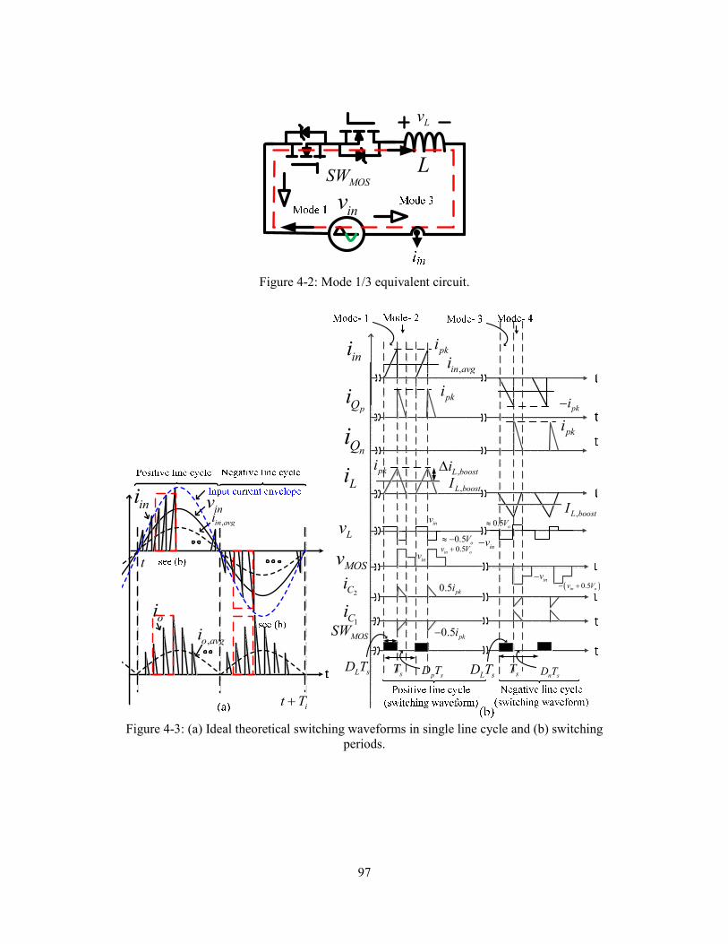
97
MOSSWL
inv
Lv
Figure 4-2: Mode 1/3 equivalent circuit.
invini
oi
,in avgi
it T+
t
,o avgi
Li
Lv
MOSSW
L sD Tp sD Ts
T
,L boosti∆,L boostI
pki
inv
pQi
ini pki
2Ci
1Ci
nQi
0.5 pki
0.5 pki−
,L boostI
L sD Tn sD Ts
T
,in avgi
pki−
0.5o
V≈ −in
v−
0.5o
V≈
MOSv inv
0.5in ov V+
inv−
( )0.5in ov V− +
pki
pki
Figure 4-3: (a) Ideal theoretical switching waveforms in single line cycle and (b) switching
periods.

98
4.3.2. Modes 2 and 4
In Mode 2, n-MOSFETs SWMOS are switched off to allow the energy stored in L to discharge into
the load, as depicted in Figure 4-4 (a). Since the total voltage across C1 and C2 is Vo, the current
charges both C2 and the battery, C1 is discharged. In this mode, VL = vin- Vo < 0; hence, the
rectifying diode Qp is forward biased for the duration DpTs in order to charge the load and ensure
validity of volt-sec balance principle. After iL reaches zero, VL = 0 and the entire converter is
essentially switched off. The identical operation with reverse inductor current flow takes place in
Mode 4 as shown in Figure 4-4 (b).
pQ
L 2C
1C
oV
1Cv
2Cv
nQ
L 1C
2C1Cv
2Cv
(a) (b)
Figure 4-4: (a) Mode 2 and (b) Mode 4 equivalent circuits of bridgeless AC/DC converter.
4.3.3. Converter Synthesized Resistor
As mentioned previously, synthesizing variable resistors is equivalent to providing mechanical
damping in the electrical domain. In this case, the equivalent variable input resistance are defined
in terms of line voltage to both envelope and average input current as envelope input resistance
and average input resistance, respectively. Before deriving the expressions for input resistances
seen from the line terminal the average input power of the proposed converter is derived as the
following
22 2 1
0
20.25
iT
inin L s in
i s
EP dt D T V L
T T
−= =∫ (4-1)
where DL is the duty cycle, Vin is line voltage amplitude, Ein is converter input energy, Ti is line
voltage period, and Ts is switching period. According to (4-1) the input power of the proposed

99
converter varies solely as a function of input voltage (assuming other parameters remain constant);
thus making it ideal for resistor synthesis.
Similarly, average input power of the synchronous boost converter, operating in DCM, is derived
as
( )222 2 1
,
0
sin0.25
21 sin
inL sin SB in L s
in
o
VD TP d V D T L
VL
V
π θθ
π θ
− = ≈
−∫
(4-2)
where Vo is load voltage and 12i
T tθ π −= . Note that the input power in (4-2) can only be
approximated, since the instantaneous term, ( ) 12 1
0sin( ) 1 sin 0.5in oA V V d
πθ θ θ π
−−= − ≈∫ when
Vin<<Vo is assumed as shown in Figure 4-5.
Figure 4-5: Approximation of input power instantaneous term with respect to step-up ratio.
The comparisons of input powers for both converters in terms of squared duty ratios are depicted
in Figure 4-6. The values adopted are L= 1 mH, Vin= 3 (V), Ts= 1 msec, Vo= 24 (V). Comparing
(4-1) and (4-2), the input power of the proposed converter is solely a function of input voltage
(assuming other parameters remain constant); thus making it synonymous to that of physical
resistor and ideal for resistor synthesis. On the contrary, input power of the synchronous boost
converter is a function of Vin and Vo, making the synthesized resistor nonlinear (when duty cycles
not properly tuned).

100
Figure 4-6: Input power comparison of proposed AC/DC converter Pin and switch mode rectifier
Pin,SB.
The average line current iin,avg and rectified current io,avg, shown in Figure 4-3(a), are obtained as
follows
2 1
,0.5
in avg in L si v D T L−=
(4-3)
2 2 1 1
,o avg in L s oi v D T L V− −= .
(4-4)
From (4-3)-(4-4), it is observed that iin,avg oscillates with respect to Ti while io,avg is summation of
both DC and second harmonics (2Ti)-1
terms. In addition, to ensure DCM operation, the
maximum duty cycle of gating pulses is also derived as
DL,max < ( ) 12
2in o in o inV V V V V−
+ . (4-5)
Combining (4-1)-(4-4), the average line resistance of the proposed converter (i.e., Rin) is defined
as follows
2
,
2
L
inin
in avg s
v LR
i D T= = . (4-6)

101
Referring to (4-6) , it is noted that Rin is solely a function of constant parameters. The envelope
input resistance is defined as the input voltage over the input current envelope. Since the
converter is operating in DCM, after L sD T , the peak value of inductor current is given by
1
pk in L si v D T L−= . (4-7)
Therefore, the envelope input resistance can be written as
_in ev
L s
LR
D T= . (4-8)
From (4-8), it is noted that1
_2
in L in evR D R−= , which is larger than the envelope input resistance by
more than a factor of two. This is expected since the converter operates in DCM.
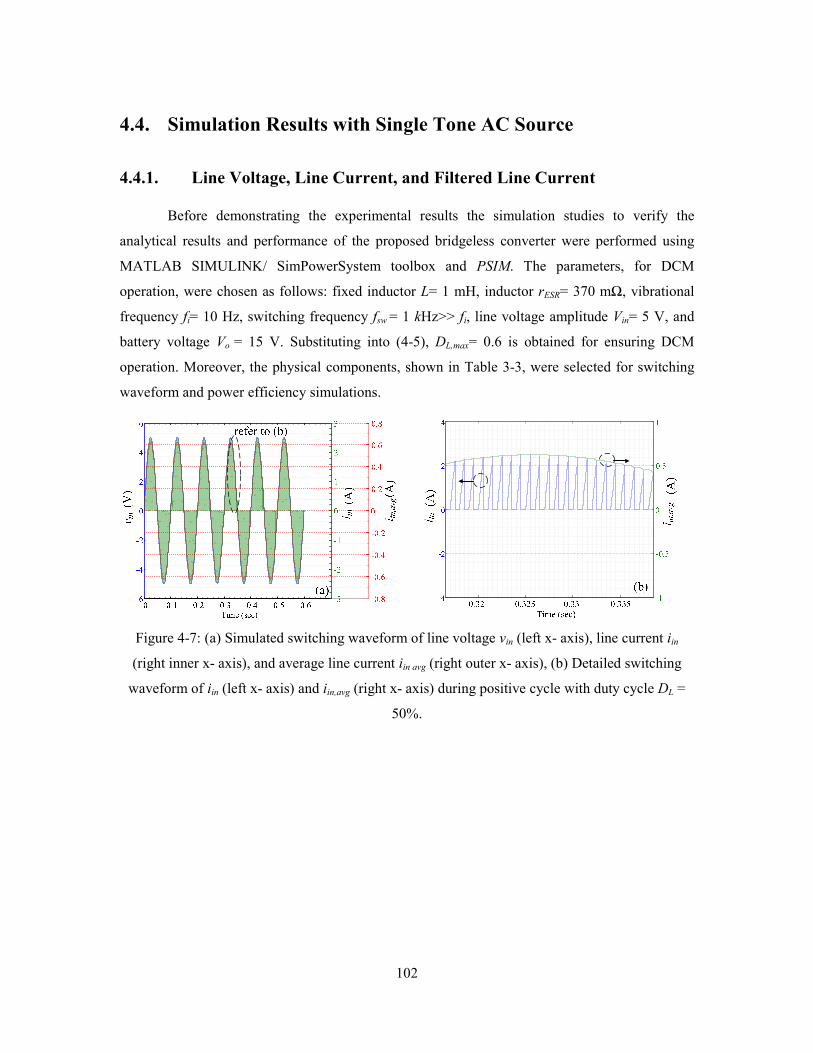
102
4.4. Simulation Results with Single Tone AC Source
4.4.1. Line Voltage, Line Current, and Filtered Line Current
Before demonstrating the experimental results the simulation studies to verify the
analytical results and performance of the proposed bridgeless converter were performed using
MATLAB SIMULINK/ SimPowerSystem toolbox and PSIM. The parameters, for DCM
operation, were chosen as follows: fixed inductor L= 1 mH, inductor rESR= 370 mΩ, vibrational
frequency fi= 10 Hz, switching frequency fsw = 1 kHz>> fi, line voltage amplitude Vin= 5 V, and
battery voltage Vo = 15 V. Substituting into (4-5), DL,max= 0.6 is obtained for ensuring DCM
operation. Moreover, the physical components, shown in Table 3-3, were selected for switching
waveform and power efficiency simulations.
Figure 4-7: (a) Simulated switching waveform of line voltage vin (left x- axis), line current iin
(right inner x- axis), and average line current iin avg (right outer x- axis), (b) Detailed switching
waveform of iin (left x- axis) and iin,avg (right x- axis) during positive cycle with duty cycle DL =
50%.
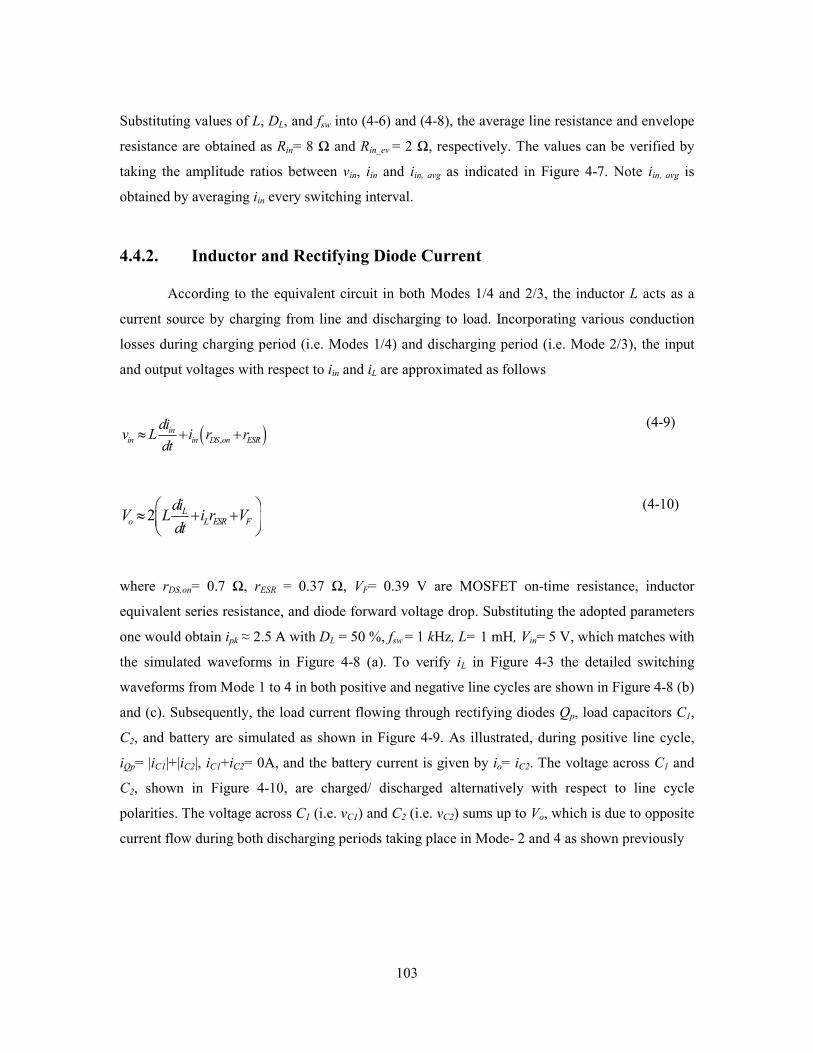
103
Substituting values of L, DL, and fsw into (4-6) and (4-8), the average line resistance and envelope
resistance are obtained as Rin= 8 Ω and Rin_ev = 2 Ω, respectively. The values can be verified by
taking the amplitude ratios between vin, iin and iin, avg as indicated in Figure 4-7. Note iin, avg is
obtained by averaging iin every switching interval.
4.4.2. Inductor and Rectifying Diode Current
According to the equivalent circuit in both Modes 1/4 and 2/3, the inductor L acts as a
current source by charging from line and discharging to load. Incorporating various conduction
losses during charging period (i.e. Modes 1/4) and discharging period (i.e. Mode 2/3), the input
and output voltages with respect to iin and iL are approximated as follows
( ),
in
in in DS on ESR
div L i r r
dt≈ + +
(4-9)
2 L
o L ESR F
diV L i r V
dt
≈ + +
(4-10)
where rDS,on= 0.7 Ω, rESR = 0.37 Ω, VF= 0.39 V are MOSFET on-time resistance, inductor
equivalent series resistance, and diode forward voltage drop. Substituting the adopted parameters
one would obtain ipk ≈ 2.5 A with DL = 50 %, fsw = 1 kHz, L= 1 mH, Vin= 5 V, which matches with
the simulated waveforms in Figure 4-8 (a). To verify iL in Figure 4-3 the detailed switching
waveforms from Mode 1 to 4 in both positive and negative line cycles are shown in Figure 4-8 (b)
and (c). Subsequently, the load current flowing through rectifying diodes Qp, load capacitors C1,
C2, and battery are simulated as shown in Figure 4-9. As illustrated, during positive line cycle,
iQp= |iC1|+|iC2|, iC1+iC2= 0A, and the battery current is given by io= iC2. The voltage across C1 and
C2, shown in Figure 4-10, are charged/ discharged alternatively with respect to line cycle
polarities. The voltage across C1 (i.e. vC1) and C2 (i.e. vC2) sums up to Vo, which is due to opposite
current flow during both discharging periods taking place in Mode- 2 and 4 as shown previously

104
Figure 4-8: (a) Simulated switching waveform of line voltage vin, inductor current iL. (b) Detailed
switching waveform during positive and (c) negative line cycle.

105
Figure 4-9: (a) Simulated switching current waveform of Qp, C1, C2, and battery current io. (b)
Detailed switching waveform during positive and (c) negative line cycle.
Figure 4-10: Capacitors voltage ripples.
4.4.3. Power Efficiency
Converter power efficiency can be calculated by measuring converter’s input and output
power. Detailed estimation of power efficiency is performed by calculating the power losses of
main converter components. The conduction/switching power losses of semiconductors and other
passive elements are estimated using PSIM as depicted by the schematic in Figure 4-11. The
thermal module allows including MOSFETs main parameters under various testing conditions
such as maximum drain–source voltage VDS_MAX, maximum drain current ID_MAX, and switching
frequency. Pre-dominant parameters such as maximum reverse recovery voltage VRRM_MAX,
maximum continuous forward current IF_MAX, and forward voltage VF can be included for diode
switching and conduction loss calculations. The power loss of passive elements can be
approximated by ESR. In addition, more detailed estimation can be performed by measuring the

106
junction thermal resistance Rth(j-c) and Rth(c-s), heat sink thermal resistance, and ambient
temperatures.
Figure 4-11: Component power loss simulation in PSIM using thermal module.
The power efficiency is generally defined as follows:
1out loss
in in
P P
P Pη = = − (4-11)
where Pout, Pin, and Ploss are the output power, input power, and power losses contributed by
physical components of the power converter.
The simulated power efficiency, shown in Figure 4-12, is obtained by both methods
indicated in (4-11). The primary contributor of total power loss comes from rectifying diode
conduction loss [59]. The results, obtained in PSIM, are plotted with respect to synthesized
resistance. As depicted, both methods demonstrate highly correlated results. The highest
conversion efficiency of ≈ 93% at Rin ≈ 22 Ω is obtained in simulation. In addition, the
experimental power efficiencies (shown in dashed line) with Rin = 10, 30, 50 Ω are arbitrarily
selected for experimental result presentation. The details are outlined in the following section.

107
Figure 4-12: Simulated and experimental power efficiency with respect to various synthesized
resistances. Note: The experimental work (black dashed line) is outlined in later sections.
4.5. Experimental Results with Single Tone AC Source
In this experiment, a programmable AC source (61501 of Chroma Systems Solutions)
was utilized as a single-phase floating AC power source. Other components adopted are tabulated
in Table 4-2. To balance the tradeoff between MOSFET on-state resistance and gate charge,
considering the general figure of merit R,DS(ON) × Qg , n-MOSFET array FDC 8602 by Fairchild
Semiconductor was selected. In general, higher R,DS(ON) leads to higher conduction power loss,
while larger Qg leads to larger switching loss due to longer turn- on and off times.
Table 4-2: Power components selected for switching waveform and power efficiency simulation.
Component Manufacture Part number
n- MOSFET Fairchild Semiconductor FDC 8602
Power Inductor Coilcraft PCV- 2- 105- 02L
Electrolytic Capacitor Nichicon UVR1J682MRD
Schottky Diode Fairchild Semiconductor MBR0520
Seal Lead- acid Battery Infinity Battery I232/ IT 1.3- 12
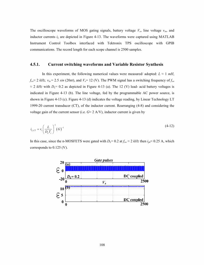
108
The oscilloscope waveforms of MOS gating signals, battery voltage Vo, line voltage vin, and
inductor currents iL are depicted in Figure 4-13. The waveforms were captured using MATLAB
Instrument Control Toolbox interfaced with Tektronix TPS oscilloscope with GPIB
communications. The record length for each scope channel is 2500 samples.
4.5.1. Current switching waveforms and Variable Resistor Synthesis
In this experiment, the following numerical values were measured/ adopted: L ≈ 1 mH,
fsw≈ 2 kHz, vin = 2.5 sin (20πt), and Vo= 12 (V). The PWM signal has a switching frequency of fsw
≈ 2 kHz with DL= 0.2 as depicted in Figure 4-13 (a). The 12 (V) lead- acid battery voltages is
indicated in Figure 4-13 (b). The line voltage, fed by the programmable AC power source, is
shown in Figure 4-13 (c). Figure 4-13 (d) indicates the voltage reading, by Linear Technology LT
1999-20 current transducer (CT), of the inductor current. Rearranging (4-8) and considering the
voltage gain of the current sensor (i.e. G≈ 2 A/V), inductor current is given by
( )1
1
,L CT t
L s
Li v G
D T
−−
=
(4-12)
In this case, since the n-MOSFETS were gated with DL= 0.2 at fsw ≈ 2 kHz then ipk≈ 0.25 A, which
corresponds to 0.125 (V).

109
Figure 4-13: (a) Gating pulses with DL= 0.2 at fsw = 2 kHz (b) load battery voltage (c) line voltage
(d) inductor current. Record Length: 2500 (points).
The detailed switching waveforms of inductor current with corresponding gating pulses and line
cycles are shown in Figure 4-14. According to (4-12), with fsw ≈ 2 kHz, DL= 0.2, |Vin|≈ 2 (V), we
should obtain peak value of inductor current ,
ˆL C Ti = + 0.1 (V) and -0.1 (V) in both positive and
negative line cycles. As indicated, the switching waveform of iL,CT ramps up/ down for charging/
discharging in both positive and negative line cycles. The non- idealities of ramp slope can be
shown by taking the KVL of the converter during on/ off durations of the MOSFETs as follows
( ),
inin in DS on ESR
div L i R r
dt≈ + +
(4-13)
2 Lo L ESR F
diV L i r V
dt
≈ + +
(4-14)
where RDS,on is the n- MOSFET on- time resistor, inductor ESR is represented by rESR, the diode
forward voltage drop is shown as VF.

110
Figure 4-14: Switching waveform of (a)- (b) detailed gating signal with corresponding inductor
current iL,CT (c)- (d) in both (e) positive and (f) negative line cycle with |Vin|≈ 2 (V).
4.5.2. Variable Resistor Synthesis
Different values of the synthesized resistor Rin can be obtained by varying DL using (4-6).
In this experiment, the switching waveforms of input current iin (i.e., inductor current during on-
time of n- MOSFETs), with DL= 0.2, 0.4, and 0.6, is shown in Figure 4-15. Again, referring to
(4-12) the voltage readings by CT should roughly correspond to 0.125 (V), 0.25 (V) and 0.375
(V), respectively.

111
Figure 4-15: Oscilloscope waveforms of iin for (a) DL= 0.2 (b) DL= 0.4, and (c) DL= 0.6. Filtered
waveforms of iin for (d) DL= 0.2 (e) DL= 0.4, and (f) DL= 0.6.
To verify the synthesized resistor Rin, iin is filtered (denoted by iin,avg) using with a second-order
low pass filter at a cutoff frequency of 500 Hz, shown in Figure 4-15 (d)- (f). Synthesized Rin can
be calculated by taking the amplitude ratio between vin and iin, avg. In this experiment, we
nominally synthesize Rin ≈ 100 Ω (Figure 4-15 (d)), 25 Ω (Figure 4-15 (e)), and 11 Ω (Figure
4-15 (f)), which can be verified by substituting into (4-6), with DL= 0.2, 0.4, and 0.6, respectively.
4.5.3. Load Capacitor Voltage
As illustrated by equivalent circuits in Figure 4-4, the voltage across C1 (i.e. vc1) and C2
(i.e. vc2) add up to Vo, which is contributed by opposite current flow during both discharging
periods taking place in Mode 2 and 4, respectively. This implies that the capacitor voltage ripples
are 180 (deg) out of phase. The sum of instantaneous voltages across capacitors C1 (i.e. vc1) and
C2 (i.e. vc2) roughly equals to 12 (V), which is the rated voltage of the load battery.
The experimental voltages across capacitors C1 and C2 along with its detailed ripples vr,c1 and vr,c2,
are shown in Figure 4-16 (a) and 10 (b), respectively. Considering the direction of inductor

112
current iL in Figure 4-4, it is observed that when C2 charges, C1 will discharge and vice versa. The
amount of capacitor voltage ripples for both C2 and C1 can be approximated as follows
1
, 1 1 10 .5r c s Cv T C i−≈ (4-15)
1
, 2 2 20 .5r c s Cv T C i−≈ . (4-16)
Due to mismatches in capacitor values and other non-idealities we can approximate vr,c1 ≈vr,c2.
Figure 4-16: (a) Load capacitor voltages and (b) corresponding ripple voltages.
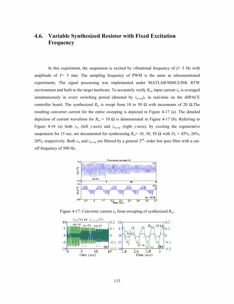
113
4.6. Variable Synthesized Resistor with Fixed Excitation
Frequency
In this experiment, the suspension is excited by vibrational frequency of fi= 5 Hz with
amplitude of Y= 5 mm. The sampling frequency of PWM is the same as aforementioned
experiments. The signal processing was implemented under MATLAB/SIMULINK RTW
environment and built to the target hardware. To accurately verify Rin, input current iin is averaged
instantaneously in every switching period (denoted by iin,avg), in real-time on the dSPACE
controller board. The synthesized Rin is swept from 10 to 50 Ω with increments of 20 Ω.The
resulting converter current for the entire sweeping is depicted in Figure 4-17 (a). The detailed
depiction of current waveform for Rin = 10 Ω is demonstrated in Figure 4-17 (b). Referring to
Figure 4-18 (a) both vin (left y-axis) and iin,avg (right y-axis), by exciting the regenerative
suspension for 15 sec, are documented for synthesizing Rin= 10, 30, 50 Ω with DL ≈ 45%, 26%,
20%, respectively. Both vin and iin,avg are filtered by a general 2nd
- order low pass filter with a cut-
off frequency of 500 Hz.
Figure 4-17: Converter current iin from sweeping of synthesized Rin.
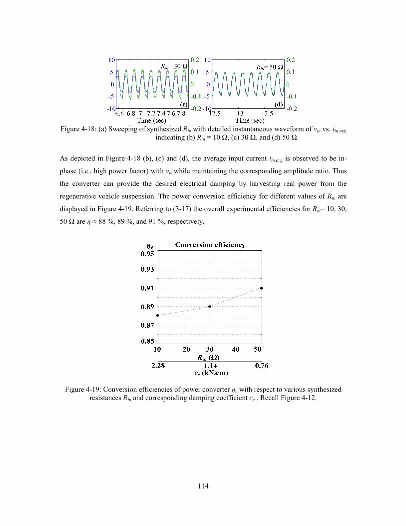
114
Figure 4-18: (a) Sweeping of synthesized Rin with detailed instantaneous waveform of vin vs. iin,avg
indicating (b) Rin = 10 Ω, (c) 30 Ω, and (d) 50 Ω.
As depicted in Figure 4-18 (b), (c) and (d), the average input current iin,avg is observed to be in-
phase (i.e., high power factor) with vin while maintaining the corresponding amplitude ratio. Thus
the converter can provide the desired electrical damping by harvesting real power from the
regenerative vehicle suspension. The power conversion efficiency for different values of Rin are
displayed in Figure 4-19. Referring to (3-17) the overall experimental efficiencies for Rin= 10, 30,
50 Ω are η ≈ 88 %, 89 %, and 91 %, respectively.
Figure 4-19: Conversion efficiencies of power converter ηe with respect to various synthesized
resistances Rin and corresponding damping coefficient ce . Recall Figure 4-12.

115
4.7. Variable Excitation Frequency with Fixed Synthesized
Resistor
The suspension prototype was excited by the MTS hydraulic actuator from fi= 5 to 10 Hz
incrementing at 0.1 (Hz/ sec) for 50 (sec). The excitation profile driving the hydraulic actuator is
shown in Figure 4-20. Similar to the experimental setup for the SMR the direct AC/DC converter
harvests the available power generated by the seismic DC machine. To verify variable resistor
synthesis by the proposed converter prototype, which is shown in Figure 4-21 (a)-(b), the line of
the converter is connected to a 1-DOF regenerative suspension system with the arrangement
shown in Figure 4-21 (c). The load is connected to rechargeable battery packs, which are
connected in series through the spade terminals are shown in Figure 4-21 (d).
0 5 10 15 20 25 30 35 40 45 50-10
-5
0
5
10
Time (sec)
mm
Excitation profile
fi= 5 Hz fi= 10 Hz
Figure 4-20: Experimental hydraulic shaker excitation profile.
(a)

116
(b)
(d)
(c)
Figure 4-21: (a) PCB components drawing of the bi-directional bridgeless AC/DC converter and
(b) its’ coreesponding prototype. (c) Experimental setup of the mechatronic system. (d) Series
SLA battery packs.
The waveforms of vin and iin,avg, obtained through the excitation profile in Figure 4-20, are
depicted in Figure 4-22. In this experiment, the synthesized resistor Rin was arbitrarily chosen as
10 Ω. Referring to Figure 4-22 (b) and (c), over the excited frequencies, average input current
iin,avg is observed to be in-phase (i.e., high power factor) with vin while maintaining the
corresponding amplitude ratio, Thus the converter can provide the desired damping in the
electrical domain by harvesting real power from the regenerative vehicle suspension. In this
experiment, the average power regenerated over fi= 5-10 Hz in 50 (sec) duration is approximately
1.73 W. Again, both vin and iin,avg are filtered by a passive 2nd- order low pass filter with a cut- off
frequency of 500 Hz.

117
Figure 4-22: Sweeping of excitation frequency for nominal Rin = 10 Ω with detailed instantaneous
waveform of vin vs. iin,avg at (b) fi ≈ 7.4 Hz and (c) fi ≈ 9.7 Hz.
4.8. Average Harvested Power
To verify maximum power transfer we repeat the same procedure depicted in Figure 4-22
for Rin= 30 Ω, 50 Ω, 100 Ω, and 200 Ω, respectively. Both instantaneous power (left z axis) and
average harvested power (right z axis) are depicted in Figure 4-23 for various Rin (x axis) swept
from fi= 3-8 Hz in 35 (sec) period.
P

118
Figure 4-23: (left Z- axis): Instantaneous and (right Z- axis): average harvested power over the
excited frequencies (i.e. 5- 10 Hz) in 35 (sec).
The average power is obtained using
( ) 1e
s
f
e s c i
f
P f f P df−
= − ∫ (4-17)
where the difference between fe and fs indicates the range of excitation frequencies fi. Referring to
Figure 3-30, Figure 4-19, and Figure 4-23, the average harvested power P (right z- xis) indicates
that the maximum power transfer takes place at Rin= 10 Ω (approximates the equivalent resistor
of the DC machine coil) and lowest overall experimental efficiency η. Recalling Figure 3-30, this
is a trade-off observed for power regeneration and conversion efficiency.
4.9. Chapter Summary
In this chapter, we proposed a sensorless direct AC/DC converter, operating in DCM, and
investigated its performance through simulation and experiments. Variable resistor synthesis and
the boundary for DCM operation were obtained along with the equivalent circuits in different
switching modes. Through detailed analysis between converter line voltage and current, the
realized converter current can be adjusted with respect to duty cycles of the bi-directional
MOSFETs; hence, accomplishing adjustable resistor synthesis. Furthermore, the converter was
placed under variable line frequency sweep for different values of synthesized resistors to
demonstrate maximum power transfer. The purpose is to show the direct AC/DC converter, with
the aforementioned benefits, when operating in DCM, is able to capture DC machine EMF,
inducted by seismic ground excitation through a small- scale suspension prototype. Through
comparison, it is noted the proposed topology offers a simplistic sensorless alternative, to that of
SMR, for capturing seismic road energy.

119
Chapter 5.
Autonomous Start/ Stop Algorithm
An electric vehicle (EV) not only drains battery power when operating, it comsumes
power even while idling or turned off. The power drain during these events may lead to battery
power loss and contributes to reduction of EV range capacities, which makes shutting off the
battery power drain beneficial over time. For a Tesla Model S, the “vampire power drain”
consumes roughly 14 (km) of range capacity, which accumulates to roughly 8000 km per year,
making the reduction of this power loss imperative for EV range extension [121]-[122]. The
mitigation of the quiescent power drain contributes to the development of “Sleep Mode” on a
Tesla Motor firmware. According to [121], the feature claims to reduce the quiescent power loss
to 0.2%.
The proposed algorithm is independent of power converter topologies. The concept of
adaptive turn on/off is applied to a SMR for demonstrating autonomous start/stop the circuit’s
operation for minimizing electrical quiescent power loss. The core of the concept is to detect the
average instantaneous input power over certain time duration and decide the optimal starting time
to operate the harvesting circuits (see Figure 5-1) for the purpose of ensuring “net-positive”
instantaneous power harvesting. Similarly, as the harvester (i.e. electromagnetic suspension) steps
out of “net- positive” region the algorithm will disable the operation of the harvesting circuits
until line voltage vx (and converter current iin) reaches minimal level. The term “net-positive” will
be explained in the following sections.

120
Figure 5-1: SMR (solid lines) with digitally implemented full- wave rectifier (dashed lines).
The term “net-positive” (i.e. Pnp), defined in (5-1), is the difference between available
instantaneous harvestable power Pin minus the sum of all power losses in a harvesting circuit Ploss
(e.g. quiescent, conduction, and switching power losses)
( ) ( )np in lossP t P t P= − (5-1)
when Pnp> 0 (Watts) the condition of net positive is met. As indicated in [122], an autonomous
energy harvesting circuit should take into account quiescent power loss (Pq) while calculating
total power loss during operation. In this work, Ploss for the SMR is the derived as
loss cond sw drv q auxP P AP BP P P= + + + + (5-2)
where the coefficients A and B are dictated by number of MOSFETs and gate drivers. Pq is the IC
quiescent power loss. Paux is the auxiliary ICs operating power consumption. The total power loss
is decomposed into conduction Pcond, switching Psw, and gate driver losses Pdrv, respectively. They
are derived as
( )2
, intcond t ds on ESRP i aR R R= + + (5-3)

121
( )0.5sw sw b t on offP f V i t t= + (5-4)
drv gs g swP V Q f= (5-5)
where Rds,on, RESR, and Rint are the drain- source on- time resistor, inductor equivalent series
resistor, and internal resistor of DC machine that represents the machine coil loss. it is the
conducting current. Vb, ton, and toff are the MOSFET blocking voltage, turn- on and off time,
respectively. Vgs and Qg are the adopted MOSFET gate- source voltage and corresponding
MOSFET gate charge. For the specific application, Psw can be neglected due to level of it and
switching delay time with adopted supply voltage (≈12 V).
As mentioned earlier, a Maxon DC motor (RE40-218011) with Rint ≈ 10 Ω > RESR >>
Rds,on was selected as the available power generator of the regenerative suspension prototype. In
the proposed algorithm, when the SMR is disabled the load battery disconnects (after a time
delay) the auxiliary circuits, therefore, making it possible for minimizing Pq. For the SMR
prototype, Paux≈ 11 mw, which is explained in much details in later sections. Moreover, since Qg≈
40 nC (at Vgs= Vds 12 V) for n- MOSFET IRFZ44N [124]. Hence, Ploss,r can be simplified as
2
, intloss r t auxP i R P≈ + . (5-6)
According to (5-6), during road excitation, the main contributor of electrical efficiency
degradation of the regenerative suspension is the internal resistance of the DC machine. While
road excitation is absent (i.e. vehicle idle), the main contributor of overall efficiency degradation
is the quiescent power loss Pq, which the proposed adaptive turn on/ off algorithm aims to
mitigate.
In order to achieve the aforementioned requirements, an emulated full- wave rectifier (FWR) with
parallel RC load has been digitally implemented (connected by dashed lines in Figure 5-1). The
FWR line voltage vx is estimated by DC machine encoder. Again, the purpose of FWR is for
achieving “net- positive” operation and autonomous turn-off as the excitation voltage source

122
exceeds and reduces to threshold level (e.g. vehicle braking/ idling), respectively. Averaging the
rectified line voltage vx results in the following
1
t T
x x
t
v T v dt+∆
−=∆ ∫ (5-7)
where ∆T is nominal duration for averaging rectified vx. In this work, ∆T = 1/60 (sec). To ensure
the SMR stays in “net- positive” region a threshold voltage Vth,, is defined in the following
1
t T
th in np
t
V R T P dt
+∆−= ∆ ∫
(5-8)
where Rin is the desired synthesized variable resistor value. The “net- positive” is established if
xv >Vth. To illustrate, assuming sinusoidal vx the time required for stepping in the “net- positive”
region is derived as follows
( )1 1 1sinc th xT V v ω− − −= (5-9)
Similarly, as vx reduces (e.g. vehicle idling) the time required to autonomously disable the
auxiliary circuit is expressed as
( )1lnd th xT V vτ −=− (5-10)
where ω is the excitation angular frequency. The discharge time constant τ=RLCL is the product of
load resistor and capacitor of the emulated FWR, respectively. It is worthy to note that since the
battery is hard switched- off, by Q5 in Figure 5-1, from the auxiliary circuit, therefore it is
imperative that it is performed after it has reduced to its’ minimum level to prevent undesired
current transients, which explains the purpose of (5-10) for delayed turn- off.

123
5.1. Auxiliary Circuit
In this work, the SMR prototype and the auxiliary circuit, powered by SLA battery, is
depicted in Figure 5-2. The main components and ICs are tabulated in Table 5-1. As depicted in
Figure 5-2 (a) and (b), the gate drivers are consisted of two floating type gate driver ICs (i.e. IR
2110), bootstrap capacitors cb, and diodes Db. According to [124]-[125], the IC quiescent power ≈
5 mw (VDD≈12 V). In addition, gate resistor Rg/ anti- parallel diodes Dg are placed for MOSFETs
slow turn- on/ fast turn off. In addition, current sensing is accomplished by a bi- directional
current sense amplifier (LT 1999- 20), which is supplied by a switch- mode voltage regulator
(P7805), as shown in Figure 5-2 (c). The pin Vout indicates the bi- directional current reading. The
pins VIN+ and VIN- connect to current sense resistor Rs. The quiescent power of LT 1999-20 and
P7805 are approximately as ≈ 7.5 mw (V+≈ 5 V) and 0.45 mW, respectively [126]-[127]. The
auxiliary circuit consumes total of Paus≈ 11 mw and Pq≈ 13 mw.
(a)
(b)
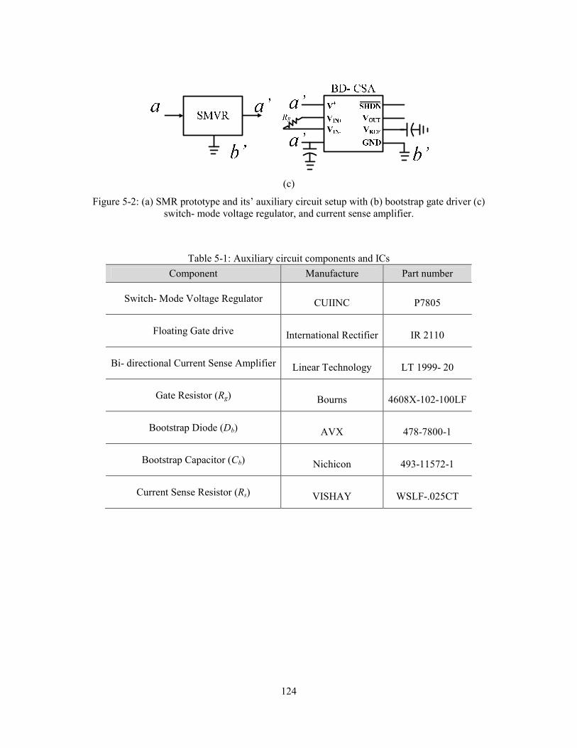
124
(c)
Figure 5-2: (a) SMR prototype and its’ auxiliary circuit setup with (b) bootstrap gate driver (c)
switch- mode voltage regulator, and current sense amplifier.
Table 5-1: Auxiliary circuit components and ICs
Component Manufacture Part number
Switch- Mode Voltage Regulator CUIINC P7805
Floating Gate drive International Rectifier IR 2110
Bi- directional Current Sense Amplifier Linear Technology LT 1999- 20
Gate Resistor (Rg) Bourns 4608X-102-100LF
Bootstrap Diode (Db) AVX 478-7800-1
Bootstrap Capacitor (Cb) Nichicon 493-11572-1
Current Sense Resistor (Rs) VISHAY WSLF-.025CT

125
Figure 5-3: State diagram of DB- HCC with additional adaptive turn on/off state.
As indicated, “net- positive” is determined by Pnp. Observing the DB- HCC state diagram
with additional adaptive turn on/off state, in Figure 5-3, it is seen that the SMR is instructed to
operate only when Pnp> 0 (i.e. xv >Vth). As a result, Q5 is gated (see Figure 5-1), SD pin (i.e. pin
11 on IR2110) is pulled to ground, and SMR is operating in DB- HCC state diagram. During this
process as xv is monitored, when
xv < Vth (caused by either vehicle braking or idling) the
operation of SMR terminates, Q5 is opened, and SD pin is gated. Consequently, the quiescent
power loss is minimized.
5.2. Adaptive Algorithm with ISO-standard Drive Cycle
In this work, a nominal driving cycle has been architected in Figure 5-4. The driving
cycle is essentially an International Standard Organization (ISO) 8608 Road class C roughness
developed at different vehicle speeds. As indicated, the vehicle is nominally chosen to accelerate
from static (0 km/h) to highest speed of 50 km/h and brake to idle.
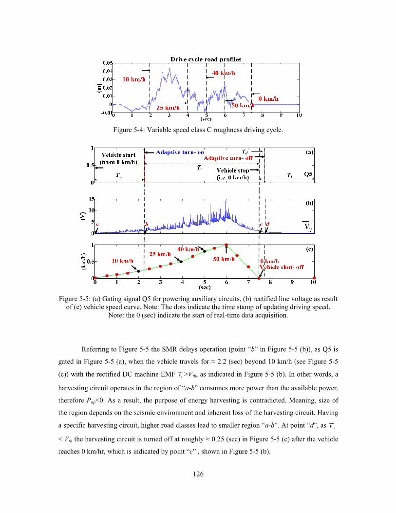
126
Figure 5-4: Variable speed class C roughness driving cycle.
Figure 5-5: (a) Gating signal Q5 for powering auxiliary circuits, (b) rectified line voltage as result
of (c) vehicle speed curve. Note: The dots indicate the time stamp of updating driving speed.
Note: the 0 (sec) indicate the start of real-time data acquisition.
Referring to Figure 5-5 the SMR delays operation (point “b” in Figure 5-5 (b)), as Q5 is
gated in Figure 5-5 (a), when the vehicle travels for ≈ 2.2 (sec) beyond 10 km/h (see Figure 5-5
(c)) with the rectified DC machine EMF xv >Vth, as indicated in Figure 5-5 (b). In other words, a
harvesting circuit operates in the region of “a-b” consumes more power than the available power,
therefore Pnp<0. As a result, the purpose of energy harvesting is contradicted. Meaning, size of
the region depends on the seismic environment and inherent loss of the harvesting circuit. Having
a specific harvesting circuit, higher road classes lead to smaller region “a-b”. At point “d”, as xv
< Vth the harvesting circuit is turned off at roughly ≈ 0.25 (sec) in Figure 5-5 (c) after the vehicle
reaches 0 km/hr, which is indicated by point “c” , shown in Figure 5-5 (b).

127
Figure 5-6: (a) inverter voltage, (b) left Y- axis: line voltage, right Y- axis: reference current, (c)
controlled input current, and (d) rectified current for battery storage
The algorithm can also be verified by observing inverter voltage vDC, line voltage vin,
reference current iref, input current iin, and rectifier current iDC. As indicated in Figure 5-6 (a) as t<
Tc, vDC equals to vin. This represents an equivalent open- circuit, meaning not only it (shown in
Figure 5-6 (c)) equals to 0 (A), theoretically, but also the auxiliary circuits are not in operation.
As t> Tc, the SMR and its auxiliary circuits are in operation. In this work, a nominal Rin= 50 Ω
has been chosen. In this mode, the iin is controlled (by DB- HCC) to synthesize Rin= 50 Ω, which
is verified through the corresponding amplitude ratio with vin (shown in Figure 5-6 (b)). The
rectified current iDC for battery storage is depicted in Figure 5-6 (d). Lastly, as vehicle becomes
idling the algorithm not only suspends the auxiliary circuit quiescent power consumption but also
actuates the shut- down (SD) pin of the gate driver, resulting vDC equals to 0 (V). For detailed
instantaneous performance of the proposed autonomous algorithm with a Q- car electromagnetic
suspension, a video of the real-time implementation was posted on [129].

128
5.3. Efficiency Enhancement
As indicated earlier, the ISO road profile is a stochastic process (non-deterministic),
which implies that the induced motor EMF does not reach a pure sinusoidal state. Therefore, to
calculate for power efficiency it is desired to normalize the averaged available power and power
loss over the entire driving cycle. To obtain the available power Pin the sum of instantaneous
input power have been normalized to the total driving cycle (see Figure 5-5 (a)) Ttot = Tc + Tr + Ti
= 10 (sec) as follows
1rt T
in tot x t
t
P T v i dt
+−= ∫
(5-11)
Recalling (5-2) - (5-6), the power efficiencies of the SMR with and without the autonomous start/
stop algorithm are written as the following, respectively
( )1 2 1
int1 /rt T
a tot t r aux d tot q in
t
T i R dt T P T T P Pη+
− −
≈ − + + ∫
(5-12)
( )1 2 1
int1 /rt T
tot t r aux tot r tot q in
t
T i R dt T P T T T P Pη+
− −
≈ − + + − ∫ (5-13)
where Tc, Tr, Td, and Ti indicate the time of adaptive turn- on time, driving time, adaptive turn- off
time, and vehicle idling time, respectively. The values for the nominal driving cycle are tabulated
in Table 5-2.
Table 5-2: Composition of Driving Cycle Time.
Driving Cycle Time Value (sec)
Total Driving Duration Ttot 10
Adaptive Turn- On Tc 2.2
Driving Tr 5.3
Adaptive Turn- Off Td 0.2

129
Driving Cycle Time Value (sec)
Vehicle Idling Ti 2.5
Rectfied Voltage Averaging Duration ∆T 1/60
Discharge Constant τ 0.01
For the adopted driving cycle, in Figure 5-5 (c), efficiency comparisons are tabulated in Table 5-3.
The converter power efficiencies (SMR) efficiency are also obtained by omitting the source
impedance of DC machine (i.e. Rint= 0 Ω). The results indicate that the efficiency improvement
for ISO 8608 class C road profile is roughly 14%. The calculations are as follows
1aIηη
≈ −
. (5-14)
Table 5-3: Comparisons of conversion efficiency with start/ stop algorithm
SMR Efficiency Power Efficiency Improvements (I)
ηa≈ 91 % ηa ≈ 76 % I≈ 14 %
η ≈ 80 % η ≈ 67 % I≈ 14 %
5.4. Chapter Summary
In this chapter, an autonomous start/ stop algorithm, for power conversion efficiency
enhancement, wa implemented to provide a method to start/stop the harvesting circuit based on
the estimated available power provided by the DC machine. Independent of vehicle velocity, the
algorithm decides the optimum point for the converter to initiate harvesting behaviour by
estimating the difference between its’ auxiliary power consumption and available power induced
by the seismic source (i.e. road). It is inherently adaptive to different road roughnesses. The

130
converter operation is ceased, with a time delay (for avoiding undesired voltage/ current
transients), after the induced EMF has diminished (e.g. vehicle idling). The start/ stop operation
the exemplifing SMR is minaly accomplished by 1. Connect/ disconnect battery powered
converter auxiliary circuits (i.e. current transducers, gate drivers, voltage regulators, etc) and 2.
Gating the shutdown (SD) pins of MOSFETs gate driver ICs. To illustrate, the power conversion
efficiency enhacement of 14% for the SMR has been documented on a class C variable speed
drive cycle.

131
Chapter 6.
Conclusions and Suggestions for Future Work
A regenerative suspension system not only allows the possibility of road energy regeneration,
but also, enables the control of vehicle sprung mass dynamics. The concept mitigates the
conventional tradeoffs between active/semi-active (e.g. Sky-hook, RS) and passive control
methods. Traditionally, active/semi-active control of a vehicle suspension system consumes
electrical power (e.g. magic body control). Suspension passive control does not consume
electrical power consumption; however, it can not accomplish variable control objectives. It is
shown, throughout this work, the purposes of controlling suspension dynamics and harvesting
road engeries can be met simultaneously, by the use of switched mode power electronics. The
switched mode converters not only harvests the regenerated power, but also, provides variable
levels of damping forces, in the electrical domain, to accomplished desired sprung mass control
performance. To conclude my work, the summaries of the accomplished tasks are outlined in the
following:
1. A regenerative suspension system prototype (i.e., SDOF system with ball- screw/DC
machine) was illustrated, in great details, with respect to sprung mass dynamics and
power harvesting. Through experimental results, different suspension dynamics scenarios
were discussed. It is noted that the smaller the equivalent load resistor is, the higher
amount of equivalent damping is provided to the suspension system. The FRF between
both sprung mass acceleration and suspension relative displacements have been provided.
2. To achieve control and energy harvesting of a regenerative suspension system, a bi-
directional SMR, controlled by DB-HCC, for variable resistors synthesis was designed,
simulated, and fabricated. The purpose of the converter is twofold: (1) To present
variable levels of electrical damping by adjusting the duty-cycles of the inverter, and (2)
Harvest the dissipated energy by using the DC machine. To examine variable electrical

132
damping, we experimentally demonstrated regeneration and motoring modes. The results
were demonstrated under variable excitation frequency and variable synthesized resistors.
Moreover, the conversion efficiency of both mechanical suspension and power converter
are identified. In addition, with the modelling of ISO road profile, the SMR is placed
under both ISO 8608 class C and D excitation for variable damping provision and energy
harvesting. According to the experimental waveforms, it is realized the converter
controlled by DB- HCC is capable of regulating the desired line current, thus presenting
the desired electrical damping.
3. In addition to constant damping, the converter is also implemented for applications in a
semi-active control algorithm (i.e. Sky-hook). Conventionally, realizing semi- active
control consumes power; the benefits of the proposed approach are towfolds: (1) Realize
Sky-hook type damping, and (2) Regenerate energy. The FRF in terms of average
regenerated power, sprung mass acceleration, and suspension relative displacement of the
regenerative modified Sky-hook is obtained. In addition, the instantaneous waveforms
indicating the converter responded to Sky-hook switching are documented. Also, the
transient response of both Sky-hook and constant damping are presented. According to
the experimental results, the DB- HCC controlled switch- mode rectifier (SMR) is able to
generate equivalent electrical dampings, according to the Skyhook detection outcome, to
the suspension system prototype. Therefore, it actively controls the suspension dynamic
while mitigates the tradeoffs between suspension passive control (lack of control) and
conventional active control (power consumption) methods.
4. A new direct AC/DC converter, operating in DCM, has been proposed. The purpose of
the converter is to provide an alternative to the SMR for the purpose of energy
harvesting. The benefits of such converter are simpler auxiliary circuit design, control,
and smaller converter foot-print. Meaning, it is also suitable for very low available
power applications (e.g. piezo-based transducer), since in such application the power
consumption of auxiliary circuits should also be taken into account. Detailed analysis
and modeling of the power converter in various switching modes were presented along
with control strategy for input resistance synthesis. The experimental switching
waveforms, such as line voltage, current, and rectified current correlated with that of
theoretical analyses. The ability of regulating converter input resistance can be utilized

133
to emulate equivalent mechanical damping with regenerative capability. Experimental
results of the converter connected to a regenerative vehicle suspension prototype for
providing desired equivalent damping through vibrational energy regeneration is
demonstrated. Furthermore, through synthesized resistor sweep over an extended range
of frequency excitation the tradeoffs between power regeneration and conversion
efficiency are also obtained experimentally.
5. An autonomous start/stop algorithm for energy harvesting power converter has been
proposed. It allows power conversion efficiency enhancement by turning on/ off the
circuit operation. According to the power level provided by the suspension prototype, the
efficiency enhancement of 14 % is reported. In short, the algorithm ensures operations in
positive conversion efficiency region. When the instantaneous road energy exceeds the
converter quiescent power loss the converter starts to operate. When the vehicle idles, the
algorithm shuts down the converter operation with a time delay for preventing undesired
transients. The feature is synonymous to that of “Sleep- Mode” on a Tesla Model S
firmware.
6.1. Suggestions for Future Work
6.1.1. A Bandwidth Enhanced Regenerative Suspension System
Recalling from Section 1.2, the generator will capture the maximum power at its resonant
frequency. The potential future work outlined in the following have demonstrated great potentials
in minimizing ground-tire relative displacements and maximizing energy harvesting in many
applications [130]-[132]. In order to, overcome the limited bandwidth of linear resonant
generator, the nonlinear strategies for the purpose of extending operating frequency region is
examined. Several published works have focus on methods of expanding the power generation
bandwidth by tuning the energy harvester where the excitation frequency is far from the
mechanical resonance frequency. For example, a coupled shunt variable capacitor across a
cantilevered piezoelectric beam for tuning the resonance frequency for the purpose of energy
harvesting in implemented in [130]. The expansion of bandwidth for power generation by
introduction parallel inductor and resistor to a piezoelectric based energy harvester is
demonstrated in [131]. A linear spring compliance with added magnetic reluctance forces for

134
providing a wider bandwidth of operation is experimentally demonstrated in [132]. A nonlinear
mechanism with hardening stiffness, which provided a greater bandwidth, is investigated in
[133].
6.1.2. Frequency Response and Jump phenomena
Recalling Section 2.1.2 one can construct the amplitude vs. frequency plot as shown in
Figure 6-1. According to [133], by applying positive (negative) cubic stiffness force into a mass-
spring system will result in bending of the amplitude frequency response curve, thus extending
the available power bandwidth of the system into higher (lower) frequency region. It is seen that
by adjusting the systems damping, stiffness, excitation amplitude different shapes and bending
directions of the curves can be observed. It is realized that the curve bends left and right while
having negative and positive α, also, the peak amplitude of the curve grows with increasing k and
decreasing µ.
Figure 6-1: Amplitude vs. frequency curve with different nonlinearity, damping, and stiffness
parameter values
The jump phenomena can be observed by looking at the amplitude vs. frequency curve in
Figure 6-1 and Figure 6-2. To observe the phenomena one can increase the excitation frequency
(with other parameters fixed) the response amplitude will follow the path of upper branch:
B’AA’ by skipping the unstable region. When the same system with different initial
conditions running at decreasing excitation frequency the response amplitude will follow the path
of lower branch: A’BB’. The phenomenon is also investigated numerically (using ODE45)
as shown in Figure 6-3. It is clearly shown with 2 different amplitude traces, which corresponds
to the bending effect in analytical simulation. Also, the jump phenomenon is observed by forward
-20 -15 -10 -5 0 5 10 15 200
0.5
1
1.5
2
2.5
3
3.5
4
4.5
σ
a
|α|increasing
k increasing,
µ decreasing
|α|increasing
|α| : stiffness, k : amplitude of
excitation, µ : damping

135
and backward sweeping of the excitation frequency with 2 different initial conditions. It is seen
that the blue curve increases in amplitude with increasing excitation frequency only until ≈2 the
jump phenomena will occur and the amplitude jumps down to ≈0.4 and decreasing. When back
sweeping the frequency the same phenomena occur but at a different point of excitation
frequency. Therefore, from the numerical simulation it is shown that the unstable region shown in
Figure 6-2 is not physically realizable.
Figure 6-2: Amplitude vs. frequency curve indicating jump phenomena
Figure 6-3: Numerical simulation of jump phenomena in amplitude
-15 -10 -5 0 5 10 15 20
0.5
1
1.5
2
2.5
3
σ
a
lower branch
backbone curve
unstable regionupper branch
B'
B
A'
A
1 1.2 1.4 1.6 1.8 2 2.2 2.4 2.6 2.8 30
0.2
0.4
0.6
0.8
1
1.2
1.4
1.6
1.8
2
σ
a
upper branch
lower branch
jump up
jump down
136
References
[1] United States Environmental Protection Agency, “Sources of Greenhouse Gas Emissions”,
[online] 2014, http://www.epa.gov/climatechange/ghgemissions/sources.html (Accessed: 30
July 2014).
[2] D. Burtaw, M. Woerman, “ US Status of Climate Change Mitigation”, [online] 2014,
http://www.rff.org/RFF/Documents/RFF-DP-12-48.pdf (Accessed: 30 July 2014).
[3] United States Department of Energy, “ One Million Electric Vehicle By 2015”, [online]
2014,
http://www1.eere.energy.gov/vehiclesandfuels/pdfs/1_million_electric_vehicles_rpt.pdf
(Accessed: 30 July 2014).
[4] CC Image courtesy of Maurizio Pesce on Flickr.
[5] CC Image courtesy of Steve Jurvetson on Flickr.
[6] M. Hanlon. “Audi's new magnetic semi-active suspension system”. Internet:
http://www.gizmag.com/go/5752/, [Oct. 02, 2014].
[7] Hybrid Cars, “ Top 10 Most Fuel Efficient Non- Hybrid Cars- 2014”, [online] 2014,
http://www.hybridcars.com/top-10-most-fuel-efficient-non-hybrid-cars-for-2014/11/
(Accessed: 30 July 2014).
[8] Hybrid Cars, “ 2013 Nissan Leaf Review”, [online] 2014, http://www.hybridcars.com/2013-
nissan-leaf-review-video/(Accessed: 30 July 2014).
[9] Honda Power Equipement,"Wattage Calculator", [online] 2014,
http://powerequipment.honda.com/generators/wattage-calculator (Accessed: 10 July 2014).
[10] Costco Wholesale," Nature Power High Output Monocrystalline Solar Panel", [online] 2014,
http://www.costco.ca/Nature-Power-High-Output-Monocrystalline-Solar-
Panel.product.100103950.html(Accessed: 30 July 2014).
[11] Go Power !," Recreational Vehicle and Marine Solar System and Inverter Selector ", [online]
2014, https://tools.carmanah.com/src.web/GoPowerCalculator.htm?state=RvDiv
(Accessed: 30 July 2014).
[12] Mercedez Benz," Magic Body Control ", [online] 2014, http://www5.mercedes-
benz.com/en/innovation/magic-body-control-s-class-suspension/ (Accessed: 30 July 2014).
[13] Suda, Yoshihiro, Shigeyuki Nakadai, and Kimihiko Nakano. "Hybrid suspension system
with skyhook control and energy regeneration (development of self-powered active
suspension)." Vehicle system dynamics 29.S1 (1998): 619-634.
[14] Lai, Chun Yu, and Wei-Hsin Liao. "Vibration control of a suspension system via a
magnetorheological fluid damper." Journal of Vibration and Control 8.4 (2002): 527-547.
[15] Shen, Y., M. F. Golnaraghi, and G. R. Heppler. "Analytical and experimental study of the
response of a suspension system with a magnetorheological damper." Journal of intelligent
material systems and structures 16.2 (2005): 135-147.
137
[16] Yao, G. Z., Yap, F. F., Chen, G., Li, W. H., and Yeo, S. H., 2002, “MR damper and its
application for semi-activecontrol of vehicle suspension system,” Mechatronics 12, 963–
973.
[17] Rakheja, S., and S. Sankar. "Vibration and shock isolation performance of a semi-active
“on-off” damper." Journal of Vibration and Acoustics 107.4 (1985): 398-403.
[18] Peng, B. B., and X. Q. Huang. "A simulation test method for a half semi-active vehicle
suspension based on the hierarchical modeling method." Vehicular Electronics and Safety,
2006. ICVES 2006. IEEE International Conference on. IEEE, 2006.
[19] Suda, Yoshihiro, Shigeyuki Nakadai, and Kimihiko Nakano. "Hybrid suspension system
with skyhook control and energy regeneration (development of self-powered active
suspension)." Vehicle system dynamics 29.S1 (1998): 619-634.
[20] Chen, Chao, and Wei-Hsin Liao. "A self-sensing magnetorheological damper with power
generation." Smart Materials and Structures 21.2 (2012): 025014.
[21] Bianchi, N.; Bolognani, S.; Corte, D.D.; Tonel, F., "Tubular linear permanent magnet
motors: an overall comparison," Industry Applications, IEEE Transactions on , vol.39, no.2,
pp.466,475, Mar/Apr 2003.
[22] Jiabin Wang; Jewell, G.W.; Howe, D., "A general framework for the analysis and design of
tubular linear permanent magnet machines," Magnetics, IEEE Transactions on , vol.35,
no.3, pp.1986,2000, May 1999.
[23] Okada, Yohji, Sang-Soo Kim, and Keisuke Ozawa. "Energy regenerative and active control
suspension." ASME 2003 International Design Engineering Technical Conferences and
Computers and Information in Engineering Conference. American Society of Mechanical
Engineers, 2003.
[24] Nakano, Kimihiko, Yoshihiro Suda, and Shigeyuki Nakadai. "Self-powered active vibration
control using a single electric actuator." Journal of Sound and Vibration 260.2 (2003): 213-
235.
[25] R.B. Goldner, P. Zerigan, “Electromagnetic Linear Generator and Shock Absorber”, US
Patent number 6952060, 2005.
[26] Tang, Xiudong, et al. "Improved design of linear electromagnetic transducers for large-scale
vibration energy harvesting." SPIE Smart Structures and Materials+ Nondestructive
Evaluation and Health Monitoring. International Society for Optics and Photonics, 2011.
[27] Wang, J.J.; Penamalli, G. P.; Lei Zuo, "Electromagnetic energy harvesting from train
induced railway track vibrations," Mechatronics and Embedded Systems and Applications
(MESA), IEEE/ASME International Conference on , vol., no., pp. 29-34, 2012.
[28] Peng Zeng; Khaligh, A., "A Permanent-Magnet Linear Motion Driven Kinetic Energy
Harvester," Industrial Electronics, IEEE Transactions on , vol.60, no.12, pp.5737-5746,
2013.
[29] Hodgins, N.; Keysan, Ozan; McDonald, AS.; Mueller, M.A, "Design and Testing of a Linear
Generator for Wave-Energy Applications," Industrial Electronics, IEEE Transactions on ,
vol.59, no.5, pp.2094,2103, May 2012.
[30] Gysen, B. L J; van der Sande, T.P.J.; Paulides, J. J H; Lomonova, E.A., "Efficiency of a
Regenerative Direct-Drive Electromagnetic Active Suspension," Vehicular Technology,
IEEE Transactions on , vol.60, no.4, pp.1384,1[3, May 2011.
[31] Xiudong Tang; Teng Lin; Lei Zuo, "Design and Optimization of a Tubular Linear
Electromagnetic Vibration Energy Harvester," Mechatronics, IEEE/ASME Transactions on ,
vol.19, no.2, pp.615,622, April 2014.
[32] Martins, Ismenio, et al. "Permanent-magnets linear actuators applicability in automobile
active suspensions." Vehicular Technology, IEEE Transactions on 55.1 (2006): 86-94.

138
[33] D. Karnopp, "Permanent Magnet Linear Motors Used as Variable Mechanical Dampers for
Vehicle Suspensions," Vehicle System Dynamics, Vol. 18, pp. 187-200, 1989.
[34] Kim, Sang-Soo, and Yohji Okada. "Variable resistance type energy regenerative damper
using pulse width modulated step-up chopper." Journal of vibration and acoustics 124.1
(2002): 110-115.
[35] Kawamoto, Y.; Suda, Y.; Inoue, H.; Kondo, T, "Modeling of electromagnetic damper for
automobile suspension," Journal of System Design and Dynamics, 1(3): 524-535, 2007.
[36] Nakano, Kimihiko. "Combined type self-powered active vibration control of truck
cabins." Vehicle System Dynamics 41.6 (2004): 449-473.
[37] Zuo, Lei, and Pei-Sheng Zhang. "Energy harvesting, ride comfort, and road handling of
regenerative vehicle suspensions." Journal of Vibration and Acoustics 135.1 (2013):
011002.
[38] Zhongjie Li; Lei Zuo; Luhrs, G.; Liangjun Lin; Yi-Xian Qin, "Electromagnetic Energy-
Harvesting Shock Absorbers: Design, Modeling, and Road Tests," Vehicular Technology,
IEEE Transactions on , vol.62, no.3, pp. 1065-1074, 2013.
[39] Zuo, Lei, et al. "Design and characterization of an electromagnetic energy harvester for
vehicle suspensions." Smart Materials and Structures 19.4 (2010): 045003.
[40] Li, Zhongjie, Zachary Brindak, and Lei Zuo. "Modeling of an electromagnetic vibration
energy harvester with motion magnification." ASME 2011 International Mechanical
Engineering Congress and Exposition. American Society of Mechanical Engineers, 2011.
[41] Choi, S. B., M. S. Seong, and K. S. Kim. "Vibration control of an electrorheological fluid-
based suspension system with an energy regenerative mechanism." Proceedings of the
Institution of Mechanical Engineers, Part D: Journal of Automobile Engineering 223.4
(2009): 459-469.
[42] Avadhany, Shakeel, et al. "Regenerative shock absorber." U.S. Patent No. 8,376,100. 19
Feb. 2013.
[43] Jazar, G. Nakhaie, et al. "Practical frequency and time optimal design of passive linear
vibration isolation mounts." Vehicle system dynamics 39.6 (2003): 437-466.
[44] Narimani, A., M. E. Golnaraghi, and G. Nakhaie Jazar. "Frequency response of a piecewise
linear vibration isolator." Journal of Vibration and control 10.12 (2004): 1775-1794.
[45] Jazar, N.G., Alkhatib, R., Golnaraghi, M.F., (2005) “Analytical Vibration Optimization of
the Linear Quarter Car,” International Journal of Vehicle Mechanics and Mobility, (Vehicle
System Dynamics).
[46] Nakhaie Jazar, G., R. Alkhatib, and M. F. Golnaraghi. "Root mean square optimization
criterion for vibration behaviour of linear quarter car using analytical methods." Vehicle
System Dynamics 44.06 (2,006): 477-512.
[47] A.A. Shabana, Theory of Vibration. Springer Science & Business Media, 1995.
[48] Hartog, Den J. et al., Mechanical Vibrations, 4th edition. Dover Publications, 1985.
[49] Nayfeh A. H. and Mook D. T., Nonlinear oscillations, Wiley, New York, 2004.
[50] THK," Ball Screw General Catelog", [online] 2014,
http://www.thk.com/sites/default/files/documents/uk_pdf/product/general/a/ee_A15.pdf
(Accessed: 31 July 2014).
[51] de Rinaldis, A.; Scherpen, J. M A, "An Electrical Interpretation of Mechanical Systems via
the Pseudo-inductor in the Brayton-Moser Equations," Decision and Control, 2005 and 2005
European Control Conference. CDC-ECC '05. 44th IEEE Conference on , vol., no.,
pp.5983,5988, 12-15 Dec. 2005.
[52] Gysen, B. L J; van der Sande, T.P.J.; Paulides, J. J H; Lomonova, E.A., "Efficiency of a
Regenerative Direct-Drive Electromagnetic Active Suspension," Vehicular Technology,
IEEE Transactions on , vol.60, no.4, pp.1384,1393, May 2011.
139
[53] Xiudong Tang; Teng Lin; Lei Zuo, "Design and Optimization of a Tubular Linear
Electromagnetic Vibration Energy Harvester," Mechatronics, IEEE/ASME Transactions on ,
vol.19, no.2, pp.615,622, April 2014.
[54] Montazeri-Gh, M.; Soleymani, M.; Hashemi, S. "Impact of Traffic Conditions on the Active
Suspension Energy Regeneration in Hybrid Electric Vehicles", Industrial Electronics, IEEE
Transactions on, On page(s): 4546 - 4553 Volume: 60, Issue: 10, Oct. 2013.
[55] B. L. J. Gysen , J. J. H. Paulides , J. L. G. Janssen and E. A. Lomonova "Active
electromagnetic suspension system for improved vehicle dynamics", IEEE Trans. Veh.
Technol., vol. 59, no. 3, pp.1156 -1163 2010.
[56] Ottman, G.K.; Hofmann, H.F.; Lesieutre, G.A., "Optimized piezoelectric energy harvesting
circuit using step-down converter in discontinuous conduction mode," Power Electronics,
IEEE Transactions on , vol. 18, no.2, pp. 696-703, 2003.
[57] Ottman, G.K.; Hofmann, H.F.; Lesieutre, G.A., "Optimized piezoelectric energy harvesting
circuit using step-down converter in discontinuous conduction mode," Power Electronics
Specialists Conference, IEEE 33rd Annual, vol.4, pp. 1988-1994, 2002.
[58] Ottman, G.K.; Hofmann, H.F.; Bhatt, A.C.; Lesieutre, G.A., "Adaptive piezoelectric energy
harvesting circuit for wireless remote power supply," Power Electronics, IEEE Transactions
on , vol.17, no.5, pp. 669-676, 2002.
[59] D'hulst, R.; Sterken, T.; Puers, R.; Deconinck, G.; Driesen, J., "Power Processing Circuits
for Piezoelectric Vibration-Based Energy Harvesters," Industrial Electronics, IEEE
Transactions on , vol.57, no. 12, pp. 4170-4177, 2010.
[60] Kim, Hyeoungwoo; Priya, S.; Stephanou, Harry; Uchino, Kenji, "Consideration of
Impedance Matching Techniques for Efficient Piezoelectric Energy Harvesting,"
Ultrasonics, Ferroelectrics and Frequency Control, IEEE Trans., vol.54, no. 9, pp. 1851-
1859, 2007.
[61] Na Kong; Dong-Sam Ha, "Low-Power Design of a Self-powered Piezoelectric Energy
Harvesting System With Maximum Power Point Tracking," Power Electronics, IEEE
Trans., vol.27, no.5, pp. 2298-2308, 2012.
[62] Shuo Cheng; Ying Jin; Yuan Rao; Arnold, D.P., "An Active Voltage Doubling AC/DC
Converter for Low-Voltage Energy Harvesting Applications," Power Electronics, IEEE
Trans. , vol.26, no.8, pp. 2258-2265, 2011.
[63] Lefeuvre, E.; Audigier, D.; Richard, C.; Guyomar, D., "Buck-Boost Converter for
Sensorless Power Optimization of Piezoelectric Energy Harvester," Power Electronics, IEEE
Tran., vol. 22, no.5, pp. 2018-2025, 2007.
[64] Lesieutre G, Ottman G and Hofmann H., "Damping as a result of piezoelectric energy
harvesting," J. Sound Vib. 269 991–1001, 2004.
[65] Zuo, Lei, and Xiudong Tang. "Large-scale vibration energy harvesting." Journal of
intelligent material systems and structures 24, no. 11 (2013): 1405-1430.
[66] Kawamoto, Y.; Suda, Y.; Inoue, H.; Kondo, T, "Modeling of electromagnetic damper for
automobile suspension," Journal of System Design and Dynamics, 1(3): 524-535, 2007.
[67] Zhongjie Li; Lei Zuo; Luhrs, G.; Liangjun Lin; Yi-Xian Qin, "Electromagnetic Energy-
Harvesting Shock Absorbers: Design, Modeling, and Road Tests," Vehicular Technology,
IEEE Transactions on , vol.62, no.3, pp. 1065-1074, 2013.
[68] Ung, C.; Moss, S.D.; Vandewater, L.A.; Galea, S.C.; Chiu, W.K.; Crew, G., "Energy
harvesting from heavy haul railcar vibrations," Intelligent Sensors, Sensor Networks and
Information Processing, IEEE Int. Conference on , vol., no., pp. 95-98, 2013.
[69] Tang, Xiudong, et al. "Improved design of linear electromagnetic transducers for large-scale
vibration energy harvesting." SPIE Smart Structures and Materials+ Nondestructive
Evaluation and Health Monitoring. International Society for Optics and Photonics, 2011.

140
[70] Wang, J.J.; Penamalli, G. P.; Lei Zuo, "Electromagnetic energy harvesting from train
induced railway track vibrations," Mechatronics and Embedded Systems and Applications
(MESA), IEEE/ASME International Conference on , vol., no., pp. 29-34, 2012.
[71] Peng Zeng; Khaligh, A., "A Permanent-Magnet Linear Motion Driven Kinetic Energy
Harvester," Industrial Electronics, IEEE Transactions on , vol.60, no.12, pp.5737-5746,
2013.
[72] Hodgins, N.; Keysan, Ozan; McDonald, AS.; Mueller, M.A, "Design and Testing of a Linear
Generator for Wave-Energy Applications," Industrial Electronics, IEEE Transactions on ,
vol.59, no.5, pp.2094,2103, May 2012.
[73] Sabzehgar, R.; Moallem, M., "Modelling and control of a boost converter for irregular input
sources," Power Electronics, IET , vol.5, no.6, pp. 702-709, 2012.
[74] Xiudong Tang; Lei Zuo, "Simulation and experiment validation of simultaneous vibration
control and energy harvesting from buildings using Tuned Mass Dampers," American
Control Conference (ACC), 2011 , vol., no., pp.3134,3139, June 29 2011-July 1 2011.
[75] Li, Peng, Chongxiao Zhang, Junyoung Kim, Liangyao Yu, and Lei Zuo., "Buck-boost
converter for simultaneous semi-active vibration control and energy harvesting for
electromagnetic regenerative shock absorber." In SPIE Smart Structures and Materials+
Nondestructive Evaluation and Health Monitoring, pp. 90570K-90570K. International
Society for Optics and Photonics, 2014.
[76] International Organization for Standardization (ISO), International Standard ISO 8608:
Mechanical vibration - Road surface profiles - Reporting of measured data, 1995.
[77] G. Rill, Road Vehicle Dynamics: Fundamentals and Modeling, CRC Press, 2011 .
[78] L. Zuo and P.-S. Zhang, "Energy harvesting, ride, comfort, and road handling of
regenerative vehicle suspensions," Journal of Vibration and Acoustics, vol. 135, 2013.
[79] US Department of Engery, " Engery Efficiency & Renewable Enrtgy, " [online] 2014,
http://www.fueleconomy.gov/feg/Find.do?action=sbs&id=32557(Accessed: 07 August
2014).
[80] Honda Power Equipement, "Wattage Calculator, " [online] 2014,
http://powerequipment.honda.com/generators/wattage-calculator (Accessed: 10 July 2014).
[81] Montazeri-Gh, M.; Soleymani, M.; Hashemi, S., "Impact of Traffic Conditions on the Active
Suspension Energy Regeneration in Hybrid Electric Vehicles," Industrial Electronics, IEEE
Transactions on , vol.60, no.10, pp.4546,4553, Oct. 2013.
[82] Rodriguez, J.; Franquelo, L.G.; Kouro, S.; Leon, J.I; Portillo, R.C.; Prats, M.AM.; Perez,
M.A, "Multilevel Converters: An Enabling Technology for High-Power
Applications," Proceedings of the IEEE , vol.97, no.11, pp.1786,1817, Nov. 2009.
[83] Shukla, A.; Ghosh, A.; Joshi, A., "Hysteresis Modulation of Multilevel Inverters," Power
Electronics, IEEE Transactions on , vol.26, no.5, pp.1396,1409, May 2011.
[84] Attaianese, C.; Di Monaco, M.; Tomasso, G., "High Performance Digital Hysteresis Control
for Single Source Cascaded Inverters," Industrial Informatics, IEEE Transactions on , vol.9,
no.2, pp.620,629, May 2013.
[85] YouTube. “Energy Harvesting from ISO standard road profile. Gdn0= 64e-
6.”. Youtube.com. [Online]. Available http://y2u.be/sOXkBfvgI8A [Accessed with Firefox:
07 August 2014].
[86] Marchesoni, M., "High performance current control techniques for applications to multilevel
high power voltage source inverters," Power Electronics Specialists Conference, 1989.
PESC '89 Record., 20th Annual IEEE , vol., no., pp.672,682 vol.2, 26-29 Jun 1989.
[87] Dahono, P.A., "New hysteresis current controller for single-phase full-bridge inverters,"
Power Electronics, IET , vol.2, no.5, pp.585,594, Sept. 2009.
141
[88] Dahono, P.A., "New current controllers for single-phase full-bridge inverters," Power
System Technology, 2004. PowerCon 2004. 2004 International Conference on , vol.2, no.,
pp.1757,1762 Vol.2, 21-24 Nov. 2004.
[89] Zare, F.; Ledwich, G., "A hysteresis current control for single-phase multilevel voltage
source inverters: PLD implementation," Power Electronics, IEEE Transactions on , vol.17,
no.5, pp.731,738, Sep 2002.
[90] Gautam, S.; Gupta, R., "Switching Frequency Derivation for the Cascaded Multilevel
Inverter Operating in Current Control Mode Using Multiband Hysteresis
Modulation," Power Electronics, IEEE Transactions on , vol.29, no.3, pp.1480,1489, March
2014.
[91] Loh, P. C.; Bode, G.H.; Tan, P-C, "Modular hysteresis current control of hybrid multilevel
inverters," Electric Power Applications, IEE Proceedings - , vol.152, no.1, pp.1,8, 7 Jan.
2005.
[92] Purohit, P.; Dubey, M., "Analysis and design of hysteresis current controlled multilevel
inverter fed PMSM drive," Electrical, Electronics and Computer Science (SCEECS), 2014
IEEE Students' Conference on , vol., no., pp.1,5, 1-2 March 2014.
[93] Bode, G.H.; Holmes, D.G., "Hysteresis current regulation for single-phase multilevel
inverters using asynchronous state machines," Industrial Electronics Society, 2003. IECON
'03. The 29th Annual Conference of the IEEE , vol.2, no., pp.1203,1208 Vol.2, 2-6 Nov.
2003.
[94] Shukla, A.; Ghosh, A.; Joshi, A. "Improved Multilevel Hysteresis Current Regulation and
Capacitor Voltage Balancing Schemes for Flying Capacitor Multilevel Inverter", Power
Electronics, IEEE Transactions on, On page(s): 518 - 529 Volume: 23, Issue: 2, March
2008.
[95] Poh Chiang Loh; Bode, G.H.; Holmes, D.G.; Lipo, T.A, "A time-based double-band
hysteresis current regulation strategy for single-phase multilevel inverters," Industry
Applications, IEEE Transactions on , vol.39, no.3, pp.883,892, May-June 2003.
[96] Loh, P.C.; Holmes, D.G.; Fukuta, Y.; Lipo, T.A, "A reduced common mode hysteresis
current regulation strategy for multilevel inverters," Applied Power Electronics Conference
and Exposition, 2003. APEC '03. Eighteenth Annual IEEE , vol.1, no., pp.576,582 vol.1, 9-
13 Feb. 2003.
[97] Xue, X.D.; Cheng, K.W.E.; Zhang, Z.; Lin, J.K.; Wang, D.H.; Bao, Y.J.; Wong, M.K.;
Cheung, N. "Investigation on parameters of automotive electromagnetic active
suspensions", Power Electronics Systems and Applications (PESA), 2011 4th International
Conference on, On page(s): 1 – 5.
[98] Xue, X.D.; Cheng, K.W.E.; Zhang, Z.; Lin, J.K.; Wang, D.H.; Bao, Y.J.; Wong, M.K.;
Cheung, N. "Study of art of automotive active suspensions", Power Electronics Systems and
Applications (PESA), 2011 4th International Conference on, On page(s): 1 – 7.
[99] Gysen, B.L.J.; van der Sande, T.P.J.; Paulides, J.J.H.; Lomonova, E.A. "Efficiency of a
Regenerative Direct-Drive Electromagnetic Active Suspension", Vehicular Technology,
IEEE Transactions on, On page(s): 1384 - 1393 Volume: 60, Issue: 4, May 2011.
[100] Hsieh, Chen-Yu; Huang, Bo; Golnaraghi, Farid; Moallem, Mehrdad, "Sky-Hook Control
for a Regenerative Suspension System," Vehicular Technology Conference (VTC Fall), 2014
IEEE 80th , vol., no., pp.1,6, 14-17 Sept. 2014.
[101] Karnopp, Dean, Michael J. Crosby, and R. A. Harwood. "Vibration control using semi-
active force generators." Journal of Manufacturing Science and Engineering 96.2 (1974):
619-626.

142
[102] Liu, Y., T. P. Waters, and M. J. Brennan. "A comparison of semi-active damping control
strategies for vibration isolation of harmonic disturbances."Journal of Sound and
Vibration 280.1 (2005): 21-39.
[103] Fallah, M.; Bhat, R.B.; Wen-Fang Xie, "Optimized Control of Semi active Suspension
Systems Using H∞ Robust Control Theory and Current Signal Estimation," Mechatronics,
IEEE/ASME Transactions on , vol.17, no.4, pp.767,778, Aug. 2012.
[104] Bai, Xian-Xu; Wereley, Norman M., "A fail-safe magnetorheological energy absorber for
shock and vibration isolation," Journal of Applied Physics, vol.115, no.17,
pp.17B535,17B535-3, May 2014.
[105] Sankaranarayanan, V.; Emekli, M.E.; Gilvenc, B.A.; Guvenc, L.; Ozturk, E.S.; Ersolmaz,
E.S.; Eyol, I.E.; Sinal, M., "Semiactive Suspension Control of a Light Commercial
Vehicle," Mechatronics, IEEE/ASME Transactions on , vol.13, no.5, pp.598,604, Oct. 2008.
[106] Zapateiro, M.; Pozo, F.; Karimi, H.R.; Ningsu Luo "Semiactive Control Methodologies for
Suspension Control With Magnetorheological Dampers", Mechatronics, IEEE/ASME
Transactions on, On page(s): 370 - 380 Volume: 17, Issue: 2, April 2012.
[107] J. J. H. Paulides , L. Encica , E. A. Lomonova and A. J. A. Vandenput "Design
considerations for a semi-active electromagnetic suspension system", IEEE Trans.
Magn., vol. 42, no. 10, pp.3446 -3448 2006.
[108] Rakheja, S., and S. Sankar. "Vibration and shock isolation performance of a semi-active
“on-off” damper." Journal of Vibration, Acoustics Stress and Reliability in Design 107, no.
4 (1985): 398-403.
[109] Shen, Y., M. F. Golnaraghi, and G. R. Heppler. "Semi-active vibration control schemes for
suspension systems using magnetorheological dampers." Journal of Vibration and
Control 12, no. 1 (2006): 3-24.
[110] Bolandhemmat, Hamidreza, Christopher M. Clark, and Farid Golnaraghi. "Development of
a systematic and practical methodology for the design of vehicles semi-active suspension
control system." Vehicle System Dynamics, 48, no. 5 (2010): 567-585.
[111] Bolandhemmat, Hamidreza, Christopher M. Clark, and Farid Golnaraghi. "Toward
Systematic Approaches to Design and Implement Vehicles Semi-Active Control
Systems." Computer Science and Software Engineering (2008): 58.
[112] Xue, X.D.; Cheng, K.W.E.; Zhang, Z.; Lin, J.K.; Wang, D.H.; Bao, Y.J.; Wong, M.K.;
Cheung, N. "Investigation on parameters of automotive electromagnetic active
suspensions", Power Electronics Systems and Applications (PESA), 2011 4th International
Conference on, On page(s): 1 – 5.
[113] Xue, X.D.; Cheng, K.W.E.; Zhang, Z.; Lin, J.K.; Wang, D.H.; Bao, Y.J.; Wong, M.K.;
Cheung, N. "Study of art of automotive active suspensions", Power Electronics Systems and
Applications (PESA), 2011 4th International Conference on, On page(s): 1 – 7.
[114] Gysen, B.L.J.; van der Sande, T.P.J.; Paulides, J.J.H.; Lomonova, E.A. "Efficiency of a
Regenerative Direct-Drive Electromagnetic Active Suspension", Vehicular Technology,
IEEE Transactions on, On page(s): 1384 - 1393 Volume: 60, Issue: 4, May 2011.
[115] Dayal, R.; Dwari, S.; Parsa, L., "Design and Implementation of a Direct AC–DC Boost
Converter for Low-Voltage Energy Harvesting," Industrial Electronics, IEEE Transactions
on , vol.58, no.6, pp.2387,2396, June 2011.
[116] D.M. Mitchell, "AC-DC Converter having an improved power factor,” U.S. Patent
4,412,277, Oct. 25, 1983.
[117] Huber, L.; Yungtaek Jang; Jovanovic, M.M., "Performance Evaluation of Bridgeless PFC
Boost Rectifiers," Power Electronics, IEEE Transactions, vol. 23, no. 3, pp. 1381-1390,
2008.

143
[118] Bowden, J, Clare, L & Burrow, S 2010, ‘Unity Power Factor Correction For
Electromagnetic Vibration Harvesters’, PowerMEMS 2010 Leuven Belgium., pp. 151 – 154,
2010.
[119] Fairchild Semiconductor, Appl. Note 9721.
[120] Linear Technology, “LT 4356-1/ LT 4356-2 Surge Stopper” LT 4356 datasheet.
[121] Green Car Reports, “Life With 2013 Tesla Model S: 'Vampire' Thirst For Electricity At
Night?”, [online] 2013, http://www.greencarreports.com/news/1082949_life-with-2013-
tesla-model-s-vampire-thirst-for-electricity-at-night. (Accessed: 5 Aug 2014).
[122] ECOMENTO, “Tesla update stops the Model S losing charge when it’s turned off”,
[online] 2013, http://ecomento.com/2013/08/19/tesla-update-stops-the-model-s-losing-
charge-when-its-turned-off/. (Accessed: 19 Aug 2014).
[123] Szarka, G.D.; Burrow, S.G.; Stark, B.H., "Ultralow Power, Fully Autonomous Boost
Rectifier for Electromagnetic Energy Harvesters," Power Electronics, IEEE Transactions on
, vol.28, no.7, pp.3353,3362, July 2013.
[124] International Rectifier, “HEXFET Power MOSFET” IRFZ44N datasheet.
[125] International Rectifier, “XPHASE3TM
Dual Phase IC” IR 3527 datasheet.
[126] International Rectifier, “HIGH AND LOW SIDE DRIVER” IR 2110 datasheet.
[127] Linear Technology, “High Voltage, Bi – directional Current Sense Amplifier” LT 1999
datasheet.
[128] CUIINC, “NON- ISOLATED SWITCHING REGULATOR” P 7805- S datasheet.
[129] YouTube. “SMR Autonamous Start/ Stop Under ISO 8608 Excitation
(2)”. Youtube.com. [Online]. Available http://y2u.be/udyR4KQSnhY [Accessed with
Firefox: 10 July 2014].
[130] Wu W J, Chen Y Y, Lee B S, He J J and Peng Y T 2006, Tunable resonant frequency
power harvesting devices Proc. SPIE 6169 61690A1- 8.
[131] Renno J M, Daqaq M F and Inman D J 2009 On the optimal energy harvesting from a
vibration source J. Sound Vib. 320 386- 405
[132] Tang, Lihua, Yaowen Yang, and Chee Kiong Soh. "Toward broadband vibration-based
energy harvesting." Journal of Intelligent Material Systems and Structures 21.18 (2010):
1867-1897.
[133] Burrow, S. G., et al. "Vibration energy harvesters with non-linear compliance."The 15th
International Symposium on: Smart Structures and Materials & Nondestructive Evaluation
and Health Monitoring. International Society for Optics and Photonics, 2008.