Energy Policy 95 (2016) 172–186

Contents lists available at ScienceDirect

Energy Policy

http://d0301-42

n CorrE-m

victor.co

journal homepage: www.elsevier.com/locate/enpol

Energy expenditure, economic growth, and the minimum EROIof society

Florian Fizaine a,n, Victor Court b,c,d

a Réseaux, Innovation, Territoires et Mondialisation (RITM), Univ. Paris-Sud, Université Paris-Saclay, 54, Boulevard Desgranges, 92330 Sceaux, Franceb EconomiX, UMR 7235, COMUE Université Paris Lumière, Université Paris Ouest Nanterre – La Défense, 200 av. de la République, 92001 Nanterre, Francec IFP Énergies Nouvelles, 1-4 av. du Bois Préau, 92852 Rueil-Malmaison, Franced Chaire Economie du Climat, Palais Brongniart, 28 place de la Bourse, 75002 Paris, France

H I G H L I G H T S

� We estimate energy expenditures as a fraction of GDP for the US, the world (1850–2012), and the UK (1300–2008).

� Statistically speaking, the US economy cannot afford to allocate more than 11% of its GDP to energy expenditures in order to have a positive growth rate.� This corresponds to a maximum tolerable average price of energy of twice the current level.� In the same way, US growth is only possible if its primary energy system has at least a minimum EROI of approximately 11:1.

a r t i c l e i n f o

Article history:Received 1 December 2015Received in revised form22 April 2016Accepted 25 April 2016

JEL classification:N7O1O3Q4Q57

Keywords:Energy expenditureEconomic growthEnergy pricesEROI

x.doi.org/10.1016/j.enpol.2016.04.03915/& 2016 Elsevier Ltd. All rights reserved.

esponding author.ail addresses: florian.fizaine@gmail.com (F. Fizurt@chaireeconomieduclimat.org (V. Court).

a b s t r a c t

We estimate energy expenditure for the US and world economies from 1850 to 2012. Periods of highenergy expenditure relative to GDP (from 1850 to 1945), or spikes (1973–74 and 1978–79) are associatedwith low economic growth rates, and periods of low or falling energy expenditure are associated withhigh and rising economic growth rates (e.g. 1945–1973). Over the period 1960–2010 for which we havecontinuous year-to-year data for control variables (capital formation, population, and unemploymentrate) we estimate that, statistically, in order to enjoy positive growth, the US economy cannot afford tospend more than 11% of its GDP on energy. Given the current energy intensity of the US economy, thistranslates in a minimum societal EROI of approximately 11:1 (or a maximum tolerable average price ofenergy of twice the current level). Granger tests consistently reveal a one way causality running from thelevel of energy expenditure (as a fraction of GDP) to economic growth in the US between 1960 and 2010.A coherent economic policy should be founded on improving net energy efficiency. This would yield a“double dividend”: increased societal EROI (through decreased energy intensity of capital investment),and decreased sensitivity to energy price volatility.

& 2016 Elsevier Ltd. All rights reserved.

1. Introduction

Debate still continues about the relative contributions of pro-duction factors to economic growth. Georgescu-Roegen (1971,1979) apart, economists have largely ignored the role of materials(e.g. metals) in the economic process. The attention paid to landvanished when modern industrial growth shifted the emphasis tocapital availability. The importance of routine labor and human

aine),

capital (knowledge, skills, etc.) has never been questioned, prob-ably simply because economics is by essence the study of a humansystem in which humans must play the leading part. The role ofenergy in the economic process has come in for much discussion.In addition to the economic literature that we will investigatemore specifically in the following subsections, the role of energy insociety has been considered from sociological and anthropological(Podolinsky, 1880; Spencer, 1880; Ostwald, 1911; Soddy, 1926;White, 1943; Cottrell, 1955; Tainter, 1988), ecological (Lotka, 1922;Odum, 1971), and historical (Pomeranz, 2000; Kander et al., 2014;Wrigley, 2016) perspectives. The economic literature on the re-lationship between energy and economic growth splits into two

F. Fizaine, V. Court / Energy Policy 95 (2016) 172–186 173

streams of research1: (i) Mainstream econometric analyses of therelationship between energy price/quantity and economic growth;and (ii) the biophysical paradigm and its approach to the economicsystem through net energy and energy-return-on-investment(EROI).

1.1. The contribution of econometrics to the energy–economicgrowth relation

1.1.1. Energy prices and economic growthHamilton (1983) was the first of a score of studies con-

centrating on the relation between energy prices (usually the oilprice) and economic growth (Katircioglu et al., 2015; Lardic andMignon, 2008). Because the oil price impacts economic growthasymmetrically,2 the classical methods of cointegration are in-effective, and more sophisticated methods are required to evaluatethe energy price–economic growth relation (Lardic and Mignon,2008; An et al., 2014). The scarcity of data on energy prices (acrossdifferent countries and over time) complicates the assessment ofthis relation. In a nutshell, this literature seems to converge to-ward a feedback relation between variations in energy price andeconomic growth (Hanabusa, 2009; Jamil and Ahmad, 2010),ranging from a negative to a positive effect depending on the levelof oil-dependency of the country under study (Katircioglu et al.,2015); and a clear negative inelastic impact of the oil price on GDPgrowth rates for net oil-importing countries. In addition, Naccache(2010) has shown that the impact of the energy price on economicgrowth depends on the origin of the oil price shock (supply, de-mand, or pure speculative shock), taking into account that therelative importance of each of these shock-drivers has variedconsiderably over time (Benhmad, 2013). When reviewing theliterature, we found that all these studies consider that the oilprice can exert a constant effect on an economy between twodates, whereas the energy intensity of this economy may ob-viously vary greatly over the same period of time. Just as thestudies rightly assume that low- and high-energy intensivecountries would not react in exactly the same way when con-fronted with increased energy prices, (because the former areclearly less vulnerable), the same point should also be taken intoaccount for a given country studied at different times. We there-fore recommend explicitly introducing energy intensity as a keyvariable in future diachronic empirical assessments of energyprice–economic growth relations.

1.1.2. Energy quantities and economic growthAnother impressive array of studies focuses on the relation

between quantities of energy consumed and economic growth.Such studies have been conducted since the seminal paper of Kraftand Kraft (1978). From this energy quantity–economic growthnexus, four assumptions have been envisaged and systematicallytested:

� A relation of cause-and-effect running from energy to economicgrowth. Studies supporting this assumption come close to the

1 In fact a third stream of research concerns theoretical economic models. Wechoose not to discuss this literature for the sake of space but one of the authors ofthe present paper has recently contributed to this field (see Court et al., 2016).

2 The asymmetric response of the economy to the variation of the oil price canbe explained by different factors such as the monetary policy, the existence ofadjustment costs, the presence of uncertainty affecting investment choices and theasymmetric response of oil-based products to oil price variations. In the case of anoil price variation, the different adjustment costs may result from sector shifts,change in capital stock, coordination problems between firms, and uncertainty.When combined, these adjustment costs can completely erase the benefits asso-ciated with a fall in the oil price. See Lardic and Mignon (2008) and also Naccache(2010) for more information.

thinking of the biophysical movement (presented in the fol-lowing subsection) and the proponents of the peak oil, becauseit gives a central role to energy in the economic process.

� A causal relation running from economic growth to energy. Inthis situation, energy is not essential and energy conservationpolicies can be pursued without fear of harming economicgrowth. This conservative view reflects the position of manyneoclassical economists for whom energy is seen as a minor andeasily substitutable production factor.

� A feedback hypothesis between energy and economic growth.� The absence of any causal relation between energy and economic

growth, which is also known as the neutrality assumption.

Unfortunately, after more than forty years of research and despitethe increasing sophistication of econometric studies, this area ofstudy has not so far led to either general methodological agreementor a preference for any of the four positions. More specifically, threeindependent literature reviews (Chen et al., 2012; Omri, 2014; Ka-limeris et al., 2014), covering respectively 39, 48, and 158 studies,have shown that no particular consensus has emerged from thisempirical literature and that the share of each assumption rangesfrom 20% to 30% of the total. Various explanations can be suggestedfor these mixed results, including the period under study, thecountries in question (the level of development affecting the re-sults), the level of disaggregation of the data (GDP or sectorial le-vels), the type of energy investigated (total energy, oil, renewable,nuclear, primary vs. final energy, exergy, etc.), the econometricmethod applied (OLS, cointegration framework, VAR, VECM, timeseries, panel or cross-sectional analysis), the type of causality tests(Granger, Sims, Toda and Yamamoto, or Pedroni tests), and thenumber of variables included in the model (uni-, bi-, or multivariatemodel) (Kocaaslan, 2013; Huang et al., 2008a,b; Wandji, 2013).

1.2. Biophysical economics and energy expenditure

1.2.1. Biophysical economicsDespite this lack of consensus about the direction of econo-

metric causality tests between energy price/quantity and eco-nomic growth, we do not think that the importance of energy ineconomics is invalidated. Suppose we try to determine the effectof energy consumption on the average speed of a car travelingbetween a series of equidistant refueling points. If we make aGranger causality test between the fuel bills obtained at each ga-soline station (representing energy consumption) and the re-corded average speed of the car (representing GDP growth), itwould probably indicate a causal relation running from the latterto the former. Indeed, the higher the speed of the car, the higherthe energy consumption (and the higher the gasoline bill). But noone can reasonably assume that energy does not play the primaryrole in propelling the car at some speed or other, and that we cancut energy consumption without affecting the car's motion. Webelieve this reasoning reinforces the third strand of thought aboutthe energy–economic growth relation grouping the various lines ofresearch in biophysical economics. Two pioneering researchers,Georgescu-Roegen (1971, 1979) and Odum (1971, 1973), respec-tively applied the laws of thermodynamics and energy accountingprinciples to the analysis of the economic system in the 1970sUnfortunately, it was not these seminal studies that alerted eco-nomics scholars and public opinion to the dependence of moderneconomies on energy, but rather the tremendous negative impactson economic growth of the two oil shocks of the same period.Even so, researchers in this field have pursued their efforts andproduced very recent syntheses (Hall and Klitgaard, 2012; Ayresand Warr, 2009; Kümmel, 2011).

(footnote continued)than the price of energy services when considering the long-run because the for-mer ignore major technological improvements. We completely agree with thisstatement and want to highlight that our work takes into account some of this

F. Fizaine, V. Court / Energy Policy 95 (2016) 172–186174

1.2.2. Energy expenditure as a limit to growthAs said previously, the two oil shocks of the 1970s were stark

reminders of the world economy's dependence on fossil energy.Energy expenditure, also called energy cost, is the quantity of eco-nomic output that must be allocated to obtaining energy. It is usuallyexpressed as a fraction of Gross Domestic Product (GDP). Murphyand Hall (2011a,b) suggest that “when energy prices increase, ex-penditures are re-allocated from areas that had previously added toGDP, mainly discretionary investment and consumption, towardssimply paying for more expensive energy”. These authors showgraphically that, between 1970 and 2007, the economy of the UnitedStates of America (US) went into recession whenever the petroleumexpenditure of the US economy exceeded 5.5% of its GDP. In addi-tion, Lambert et al. (2014) suggest that in the US once energy ex-penditure rise above 10% of GDP recessions follow.

Bashmakov (2007) makes a difference between energy cost toGDP ratio and energy cost to final consumer income ratio. Heidentifies energy cost to GDP thresholds of 8–10% for the US (4–5%for final consumer income) and 9–11% for the OECD (4.5–5.5% forfinal consumer income) below which he finds almost no correlationbetween the burden of energy expenditure and GDP growth rates.However, when these thresholds are exceeded, the economy slowsdown and demand for energy falls until the energy cost to GDP/consumer income ratios are back below their thresholds. Bashmakov(2007) argues that until the share of energy expenditure reaches itsupper critical threshold, it is all the other production factors thatdetermine the rates of economic growth, and energy does not per-form a “limit to growth” function. “But when energy costs to GDPratio goes beyond the threshold, it eliminates the impact of factorscontributing to the economic growth and slows it down, so thepotential economic growth is not realized”.

King et al. (2015b) estimate energy expenditures as a fraction ofGDP for the period 1978–2010 for 44 countries representing 93–95% ofthe gross world product (GWP) and 73–79% of the IEA's listed worldTotal Primary Energy Supply (TPES) (478% after 1994). The metho-dology used by these authors is set out in full in their article but itshould be pointed out that they consider coal, oil, and natural gas forthree sectors (industrial, residential, and electricity production), plusnon-fossil (nuclear, renewable) electricity production for two sectors(industrial and residential). The quantities and prices of these differentcommodities were mostly retrieved from databases of the US EnergyInformation Administration (EIA). King et al. (2015b) aggregate thesenational energy costs to estimate the global level of energy ex-penditure from 1978 to 2010. They find that this estimated energycost as a fraction of the GWP fell from a maximum of 10.3% in 1979 to3.0% in 1998 before rising to 8.1% in 2008. King (2015) uses these datato perform simple econometric correlation (hence not causal) analysesthat deliver the following main results: expenditure on energy ex-pressed as a fraction of GDP is significantly negatively correlated withthe one-year lag of the annual changes in both GDP and total factorproductivity, but not with the zero-year lag of these same variables.

1.3. Missing perspective, goal, and content

As already stressed, the various energy expenditures estimatedby King et al. (2015b) were only for the period 1978–2010, and theeconometric analyses of King (2015) were not designed to inferany temporal causality between energy expenditure and economicgrowth, nor to estimate any potential threshold effect in such arelation. Consequently, we seek to achieve two related goals in thepresent paper. First, we think it is important to extend energyexpenditure estimates (as fractions of GDP) to a larger time frame,for as many countries as possible.3 In the present paper we are

3 Fouquet (2011) highlights the danger of focusing on the price of energy rather

able to do this adequately for the US and the global economy from1850 to 2012, and for the United Kingdom (UK) from 1300 to2008.4 Second, we wish to relate the level of energy expenditureas a fraction of GDP to the economic growth dynamics in order toquantitatively support the various qualitative results previouslyadvanced by Murphy and Hall (2011a,b), Lambert et al. (2014) andKing (2015). More precisely, focusing on the US due to the avail-ability and consistency of data, we seek to:

� Perform Granger causality tests to identify the direction of thepossible causal relation between energy expenditure and GDPgrowth.

� Estimate the ultimate level of energy expenditure (as a fractionof GDP) above which economic growth statistically vanishes.

� Express this result in terms of the maximum average price ofenergy and the minimum societal energy-return-on-investment(EROI) that must prevail in the economy in order for economicgrowth to be positive.

The methodology used to estimate the level of energy ex-penditure as a fraction of GDP is developed in Section 2. In thatsection we also present the different equations necessary to esti-mate the ultimate energy expenditure level above which economicgrowth statistically vanishes, and translate this result into themaximum tolerable energy price and minimum required EROI ofsociety. We then succinctly present the logic of Granger causalitytests. In Section 3, we first show graphically our estimates of thelevel of energy expenditure as a fraction of GDP for the US and theworld economy from 1850 to 2012. Then, we give, for the US only,our estimation of the ultimate level of total energy expenditure (asa fraction of GDP) above which economic growth seems statisti-cally impossible. We then express this result as the maximumtolerable aggregated energy price (and oil price), or in otherwords, the minimum energy-return-on-investment (EROI), thatthe energy sector must have in order for the US economic growthto be positive. We then give the results of the various Grangercausality tests for the restricted 1960–2010 period for which dataare continuous and consistent. In Section 4, we discuss ourmethodology and perform some sensitivity analysis of our results.We also compare our energy expenditure estimates for the US andworld with the one for the UK calculated from 1300 to 2008 usingdata from Fouquet (2008, 2011, 2014). Finally, in Section 5, weconclude and propose some research perspectives that would beworth investigating as an extension of the present work.

2. Methods

2.1. Estimating energy expenditure

2.1.1. Equations and boundaryWe note Xj the level of expenditure of a given energy j pro-

duced in quantity Ej and sold at price Pj in a given economy:

= ( )X P E . 1j j j

In our study, the j energy forms include the following marketedenergy: coal, crude oil, natural gas, non-fossil electricity (i.e. nuclearand renewable electricity from hydro, wind, solar, geothermal,

technological progress through the energy intensity of the economy.4 Naturally, the geographical definition of the “United Kingdom” is quite blur-

red over such long time span (see Fouquet, 2008 for details).

F. Fizaine, V. Court / Energy Policy 95 (2016) 172–186 175

biomass and wastes, wave and tidal) and modern biofuels (ethanoland biodiesel). Hence, total expenditure of marketed energy,Xtotal marketed, is:

∑= =( )

X X P E .2

total marketedj

j average total marketed

With Paverage as the quantity-weighted average price of ag-gregated marketed energy:

∑=∑ ( )

P PE

E,

3average

jj

j

j j

and Etotal marketed the total supply of marketed energy:

∑=( )

E E .4

total marketedj

j

Usually, such estimates of marketed energy expenditure omittraditional biomass energy (woodfuel, crop residues5) becausethey usually represent non-marketed consumption for whichaverage annual prices cannot be estimated. Consequently, if suchan energy resource is omitted from Eqs. (1) and (2), we necessarilyunderestimate contemporary levels of energy expenditure sincewoodfuel and crop residues still represent 70% of global renewableenergy consumption nowadays (whereas hydro accounts for 20%and new renewable technologies such as wind power, solar PV,geothermal, wave, tidal, wastes, and modern biofuels account forthe remaining 10%). But most importantly, for times prior to the1940s when traditional biomass represented a large share of thetotal primary energy supply of many countries, we need a proxyfor total energy expenditure including non-marketed energies inorder to have a more accurate idea of the actual level of totalenergy expenditure. With Etrad as the quantity of traditional bio-mass energy, and = +TPES E Etotal marketed trad as the total primaryenergy supply, we define, for a given economy, the proxy of totalenergy expenditure, Xtotal proxy, as:

( )=− ( )

XX

1.

5total proxy

total marketedETPES

trad

In our results we will present a (second best) estimate of totalenergy expenditure for the US and world economy using the “totalproxy method” in order to test its consistency with the (first best)estimate which includes woodfuel as marketed energy.

2.1.2. Data for the USWe used several sources summarized in Table 1 in order to

estimate the prices of coal, crude oil, gas, electricity, woodfuel, andmodern biofuels consumed in the US.

In order to express all energy prices in the same convenientunit, i.e. International Geary-Khamis 1990 dollar6 per terajoule(abbreviated $1990/TJ), we used the US Consumer Price Index ofOfficer and Williamson (2016) and different energy conversionfactors from British Petroleum (2015) such as the average energycontent of one barrel of crude oil (5.73E�03 TJ), the average en-ergy content of one metric tonne of hard coal (29.5E�03 TJ), theaverage energy content of one thousand cubic feet of natural gas(1.05E�03 TJ), the average energy content of one gasoline gallonequivalent (1.2E�04 TJ), the average energy content of one thou-sand board feet of wood (2.3E�02 TJ), and the terajoule equivalent

5 Formally, fodder supplied to draft animals should be added to traditionalbiomass energy estimates, but it is generally discarded due to difficulties of esti-mation. This is also the case for traditional windmills and water wheels.

6 The International Geary–Khamis 1990 dollar (properly abbreviated Int. G-K.$1990), more commonly known as the international dollar, is a standardized andfictitious unit of currency that has the same purchasing power parity as the U.S.dollar had in the United States in 1990.

of one kWh (3.6E�06). We present in Fig. 1 the resulting prices ofcoal, oil, gas, electricity, and woodfuel expressed in $1990/TJ(biofuels prices are omitted from this figure for the sake of clarity).

US energy consumption levels were retrieved from EIA (2011, p.341) prior to 1950 and then EIA (2016b, p. 7) from 1949 to 2012.The nominal US GDP and deflator estimates were retrieved fromJohnston and Williamson (2016) in continuous year-to-year timeseries from 1850 to 2012.

2.1.3. Data for the worldIt is of course quite complicated to estimate the average annual

price of a given energy type at the global scale. To be accurate in suchestimations, one should formally have all national energy prices andconsumption quantities and compute for each year a quantity-weighted average price of each energy. Given the broad time frame ofour analysis, such estimation is simply impossible. Consequently, wewill use the different energy prices estimated for the US as globalproxies by considering that international markets are competitiveand that large spreads between regional energy prices cannot last forlong due to arbitrage opportunities. This assumption is fairly relevantfor oil and gas. On the other hand, the hypothesis that the averageinternational prices of coal, electricity, woodfuel, and modern bio-fuels follow their US equivalents is a rather coarse assumption. Forinstance, in the case of coal, transportation costs over long distancescan be very high so that spreads between prices of two differentexporting countries have necessarily occurred in the past. Further-more, by using a single price for coal, we ignore the manifold qua-lities of coal (from the high energy content of anthracite to the lowestquality of lignite). As our coal price estimate is representative ofanthracite, our coal expenditure estimates are probably high esti-mations of the actual levels of coal expenditure because we surelyslightly overestimate the exact quality-weighted global average priceof coal. Computing such a quality-weighted global average price ofcoal would be possible if we knew both the proportions of all thedifferent coal qualities in the total global coal production (i.e. thequality mix of the global coal supply) and their respective prices, foreach year between 1850 and 2012. As far as we know, such data isunfortunately not available.

We retrieved global primary energy productions through theonline data portal of The Shift Project (2015) which is built on theoriginal work of Etemad and Luciani (1991) for 1900–1980 and EIA(2014) for 1981–2012. Prior to 1900, we completed the differentfossil fuel time series with the original five-year interval data ofEtemad and Luciani (1991) and filled the gaps by linear interpola-tion. The work of Fernandes et al. (2007) and Smil (2010) was usedto retrieve historical global consumption of traditional biomass en-ergy (including woodfuel and crop residues but excluding fodderand traditional windmills and water wheels). The gross world pro-duct (GWP) we used comes from Maddison (2007) for 1850–1950and from the GWP per capita of The Maddison Project (2013) mul-tiplied by the United Nations (2015) estimates of the global popu-lation for 1950–2010. In order to obtain GWP estimates for 2011 and2012 we used the real GWP growth rate of the World Bank (2016a).

2.2. Estimating the maximum level of energy expenditure, the max-imum tolerable price of energy, and the minimum EROI of society

In this section we present the methodology used to estimatethe maximum level of energy expenditure above which economicgrowth cannot be positive. Then, we show how to translate thisresult into the maximum tolerable price of energy, or in otherwords, the minimum EROI of society. Although we are prettyconfident in using US energy prices as global proxies for esti-mating the global level of energy expenditure, the followingequations and econometric tests will only be applied to the US dueto the lack of availability, consistency, and confidence that we have

Table 1Sources and original units of the different prices of energies consumed in the US.

Energy Time and spatial coverage Source Original unit

Coal 1850–2012: US average anthracite price. US Census Bureau (1975a, p. 207–209) from 1850 to 1948; EIA(2011, p. 215) from 1949 to 2011; EIA (2012, p. 54) for 2012.

Nominal $US/80-lb from 1800 to 1824;then nominal $US/short tona.

Oil 1861–1944: US average; 1945–1983: ArabianLight posted at Ras Tanura; 1984–2012: Brentdated.

British Petroleum (2015) for the entire period. Nominal $US/barrel.

Gas 1890–2012: US average price at the wellhead. US Census Bureau (1975a, p. 582–583) from 1890 to 1915;Manthy (1978, p. 111) from 1916 to 1921; EIA (2016a) from 1922to 2012.

Nominal $US/thousand cubic feet.

Electricity 1907–2012: US average retail price. US Census Bureau (1975b, p. 827) from 1907 to 1959; EIA (2016b,p. 141) from 1960 to 2012.

Nominal $US cents/kW h

Woodfuel 1850–2012: US average Howard and Westby (2013, p.67); all commodities Warren andPearson (1933); Manthy (1978, p. 90).

Nominal $US/thousand board feet

Biofuels 2000–2012: US ethanol (E85). 2002–2012: USbiodiesel (B20).

US Department of Energy (2016) Nominal $US/Gasoline GallonEquivalentb

a 1 metric tonne¼1000 kg¼1.10231 short ton; 80-lb¼36.29 kg.b 1 Gasoline Gallon Equivalent¼114,100 BTU.

0

20

40

60

80

100

120

0

2000

4000

6000

8000

10000

12000

14000

16000

1850 1870 1890 1910 1930 1950 1970 1990 2010

His

toric

al p

rice

of e

lect

ricity

(Tho

usan

d $1

990/

TJ)

His

toric

al p

rice

of fo

ssil

ener

gyan

d w

oodf

uel (

$199

0/TJ

)

Time (year)

Coal Oil Gas

Wood Electricity

Fig. 1. Estimations of US energy prices for coal (1850–2012, left scale), oil (1860–2012, left scale), gas (1890–2012, left scale), woodfuel (1850–2012, left scale) andelectricity (1907–2012, right scale) in $1990/TJ.

F. Fizaine, V. Court / Energy Policy 95 (2016) 172–186176

in global estimates of population and capital formation (as afraction of GWP). Indeed, continuous population estimates arereadily available for the US for the entire period of study of thisarticle, whereas continuous estimates of global population areonly available since 1950. Regarding gross capital formation as afraction of GDP, the World Bank (2016b) proposes estimates from1960 to 2013 for the US, but only from 1970 to 2013 for the globaleconomy. Moreover, confidence in data is logically higher for awell-administered nation like the US than for global estimates.

2.2.1. Multivariate linear regressions of economic growth on energyexpenditure, capital formation, and labor availability

In the US case, once total expenditure of marketed energy( Xtotal marketed) is computed, we can perform different multivariatelinear regressions. The US GDP growth rate (obtained from John-ston and Williamson, 2016) representing the dependent variablecan be regressed on several explanatory variables, namely: energyexpenditure as a fraction of GDP (in which all marketed energyforms can be considered, or just a subset such as oil), capital for-mation as a fraction of GDP (retrieved from the World Bank,2016b), and the US population (from Johnston and Williamson,2016). As we suspect population to be a poor proxy for laboravailability, we will also test in our regressions the explanatorypower of the US unemployment rate (provided by the Bureau ofLabor Statistics, 2016). The general formula of the multivariatelinear regression we study is:

α θ θ θ= + + + ∆ ( )GDPGDP

XGDP

Capital formationGDP

Population, 6total marketed

1 2 3

whereGDP

GDPis the US economic growth rate, α is the intercept, θ1

(for which we logically anticipate a negative value) represents thesensitivity of the economic growth rate to the level of energy ex-penditure as a fraction of GDP, θ2 is the sensitivity of the economicgrowth rate to the capital formation as a fraction of GDP, and θ3 isthe sensitivity of the economic growth rate to population firstdifference ∆Population. It is important to point out that the mainadvantage of our approach is that it takes into account both theimpact of energy prices and energy efficiency on economicgrowth. Indeed, it should be remembered that energy expenditureas a fraction of GDP can be broken down as the average price ofenergy times the energy intensity (inverse of energy efficiency) ofthe economy:

=∑

= ×∑

= ( )X

GDP

P E

GDPP

E

GDPP EI, 7

total marketed j j javerage

j javerage

where EI is the energy intensity of the economy. So, rather thanconsidering only the impact of energy price or energy quantityfluctuations on economic growth, as is usually done in econo-metric studies, we suppose here that energy prices impact theeconomy variously, depending on the energy efficiency of theeconomy. The higher the energy intensity of the economy, thehigher the negative impact of energy price increases.

2.2.2. Maximum tolerable level of energy expenditureUsing Eq. (6), it is easy to find the particular value of US energy

expenditure (as a fraction of GDP) that leads to zero economicgrowth. In other words, we can define the maximum level of en-ergy expenditure (as a fraction of GDP) above which positiveeconomic growth is impossible. We call βtotal this maximum levelof energy expenditure, with:

βα θ θ

θ= =

− − − ∆

( )⎛⎝⎜

⎞⎠⎟

XGDP

Population.

8totaltotal marketed

max

Capital formationGDP2 3

1

2.2.3. Maximum tolerable quantity-weighted average price of energyDefining the maximum level of energy expenditure above

which positive economic growth is impossible can be re-formulated as the maximum aggregated price of marketed energyPaverage max that the economy can tolerate to still present a slightlypositive growth rate. Of course, this hypothetical maximum tol-erable price of aggregated energy depends on the energy intensityof the US economy as shown in (9):

F. Fizaine, V. Court / Energy Policy 95 (2016) 172–186 177

β=

( )P .

9average max

totalE

GDPtotal marketed

2.2.4. Minimum EROI required to enjoy positive economic growthConsiderable research has been conducted into the concept of

energy-return-on-investment (EROI) of human societies since allorganisms or systems need to procure at least as much energy asthey consume in order to continue in existence. The EROI is theratio of the quantity of energy delivered by a given process to thequantity of energy consumed in that same process. Hence, theEROI is a measure of the accessibility of a resource, meaning thatthe higher the EROI, the greater the amount of net energy deliv-ered to society in order to support economic growth (Hall et al.,2014). King et al. (2015a) point out that this definition is ratherloose and that a clear distinction should be made between yearly“power return ratios” (PRRs) of annual energy flows and “energyreturn ratios” (ERRs) of full life cycle energy systems (i.e. cumu-lated energy production divided by total lifetime invested energy)which more formally represent EROIs. Understandably, energyreturn ratios represent integrals of power return ratios over theentire life cycle of the energy system under consideration.

Following King and Hall (2011), an estimate of the yearly or“instantaneous” EROI of a given economy (taking into account onlymarketed energies for which prices are available) can be expressedas a function of the quantity-weighted average price of aggregatedmarketed energy, Paverage, the average monetary-return-on-invest-ment (MROI) of the energy sector (i.e. its gross margin), the grossdomestic product (GDP), and the total supply of marketed energyEtotal marketed:

=× ( )

EROIMROI

P.

10averageE

GWPtotal marketed

If we replace Paverage in (10) by the expression (9) of Paverage max,we obtain an expression of the EROImin, which is the minimumsocietal EROI that the energy system must have in order for theeconomy to enjoy a positive rate of growth:

β=

( )EROI

MROI.

11min

total

2.2.5. Robustness of econometric regressions and auxiliary testsAll of our estimations were preceded by unit root tests in order

to check the stationarity of our time series and avoid spuriousregressions. For the various estimations of energy expenditure, theAugmented Dickey Fuller test (ADF) provides conflicting resultswith the KPSS test. When we observe the residuals of the auxiliaryregressions of ADF, it seems that the outcome of the test is biasedby two important outliers occurring in 1974 and 1979 (years of oilshocks). If we introduce two dummy variables to capture this ef-fect, or if we start the test after the oil shocks, the ADF test in-dicates that the various estimations of energy expenditure as afraction of GDP are stationary. Except for the US population, thetests indicate that all other variables (US GDP growth rate, UScapital formation as a fraction of GDP, and US unemployment rate)are stationary. To save space, outcomes for unit root tests are re-ported in the Appendix.

Concerning econometric regressions, we report systematicallydifferent tests for the residuals of the estimations, especially testsof autocorrelation (Durbin-Watson7), homoscedasticity (Whiteand Arch tests), and normality of residuals (Jarque-Bera and

7 The correlogram of residuals is also checked in order to detect higher order ofautocorrelation.

Shapiro-Wilk tests). When one of the tests converges toward theassumption of autocorrelation or heteroscedasticity, we use theWhite heteroscedasticity-consistent standard errors and covar-iance matrix in order to obtain robust standard errors. The stabilityof the econometric coefficients across time is also checked byperforming the CUSUM test and the CUSUM squared tests.

2.3. Testing for Granger causality

The last part or our work consists in studying the temporalcausality between US energy expenditure (as a fraction of GDP)and US GDP growth rates between 1960 and 2010. There are manycausality tests based on different definitions of causality, but themain idea of the Granger (1969) causality test is to verify thatadding past data of variable X1 to past data of variable Y enhancesthe prediction of present values of variable Y. If the residualsgenerated from a model with variable Y and its past only, and fromanother model with the past of variable Y and the past of variableX1 are significantly different, we can reject the assumption of non-causality from X1 to Y and accept the assumption of a causalityrunning from X1 to Y. Formally, it consists in running the followingWald test:

∑ ∑ ∑

∑

θ θ

δ θ θ

θ

∀ ∈ [ … ] = ∃ ∈ [ … ] ≠ = +

+ + +

+ϵ( )

=

=

−=

=

−=

=

−

=

=

−

H i k and H i k Y c

Y X X

X

: 1, , , 0 : 1, , , 0,

.12

i i t

i

i k

i t ii

i k

i t ii

i k

i t i

i

i k

i t i t

0 1, 1 1,

1 11, 1,

12, 2,

13, 3,

We also test the assumption that all the Xj variables are not Grangercausing the variable Y by testing θ θ θ∀ ∈[ … ] = = =H : i k1, , , 0i i i0 1, 2, 3, , and

θ∃ ∈[ … ]∪ ∈ [ … ] ≠H i k j: 1, , 1, , 3 , 0j i1 , .

3. Results

3.1. US and global energy expenditure from 1850 to 2012

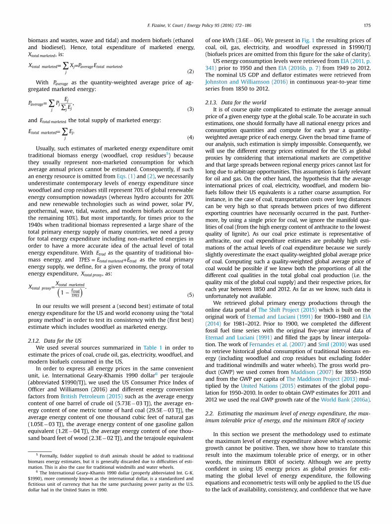
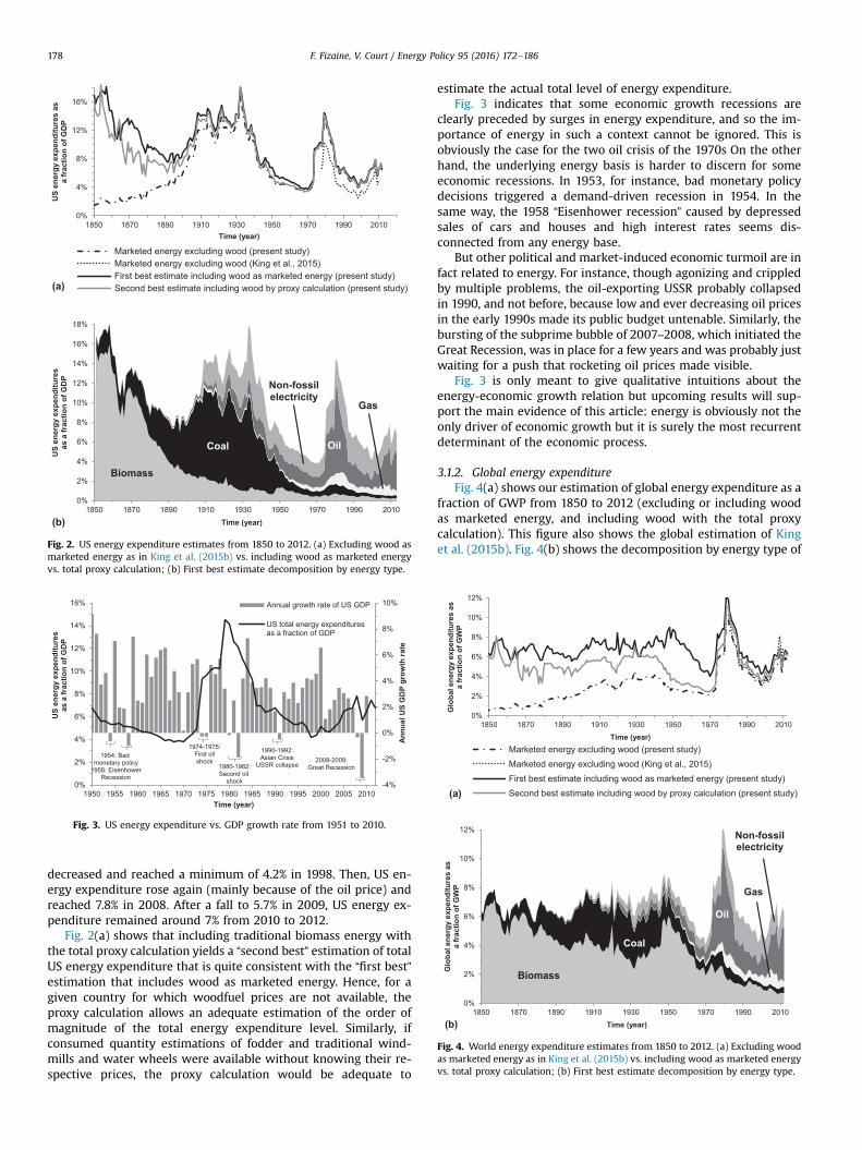
3.1.1. US energy expenditureIn Fig. 2(a) we compare three different estimates of US energy

expenditure as a fraction of GDP from 1850 to 2012 (excluding orincluding wood as marketed energy, and including wood with thetotal proxy calculation). We also show in this figure the US esti-mation of King et al. (2015b). Fig. 2(b) shows the decomposition ofour first best estimate (including wood as marketed energy) byenergy type. In Fig. 3 we relate graphically our first best estimationof the US level of energy expenditure (as a fraction of GDP) to theGDP growth rate from 1951 to 2010.

Quite logically, in early industrial times the US level of energyexpenditure was low for fossil energy (coal, oil, and gas) and non-fossil electricity. In 1850 woodfuel expenditure still represented14% of the US GDP when the overall energy expenditure level was16%. The low price of coal (cf. Fig. 1) explains that total energyexpenditure decreased from 1850 (16%) to the 1900s (8%) despite ahuge increase in consumption. From 1910 to 1945, total energyexpenditure was about 14% of GDP because of ever-increasing(cheap) coal use and the newly increasing consumption of (ex-pensive) hydroelectricity. From 1945 to 1973, which was the per-iod of highest economic growth rates for the US and all other in-dustrialized economies, the level of energy expenditure steadilydeclined from about 8% to 4%. In 1974 US energy expendituresurged to 10% of GDP, and in 1979 it reached 14.5%. These well-known periods, respectively called the first and second oil crisis,pushed industrialized economies into major recessions. After thebeginning of the 1980s, the level of US energy expenditure

0%

4%

8%

12%

16%

1850 1870 1890 1910 1930 1950 1970 1990 2010

US

ener

gy e

xpen

ditu

res

asa

frac

tion

of G

DP

Time (year)

Marketed energy excluding wood (present study)Marketed energy excluding wood (King et al., 2015)First best estimate including wood as marketed energy (present study)Second best estimate including wood by proxy calculation (present study)(a)

0%

2%

4%

6%

8%

10%

12%

14%

16%

18%

1850 1870 1890 1910 1930 1950 1970 1990 2010

US

ener

gy e

xpen

ditu

res

as a

frac

tion

of G

DP

Time (year)

Biomass

OilCoal

Non-fossilelectricity

Gas

(b)

Fig. 2. US energy expenditure estimates from 1850 to 2012. (a) Excluding wood asmarketed energy as in King et al. (2015b) vs. including wood as marketed energyvs. total proxy calculation; (b) First best estimate decomposition by energy type.

-4%

-2%

0%

2%

4%

6%

8%

10%

0%

2%

4%

6%

8%

10%

12%

14%

16%

1950 1955 1960 1965 1970 1975 1980 1985 1990 1995 2000 2005 2010

Annu

al U

S G

DP

grow

th ra

te

US

ener

gy e

xpen

ditu

res

as a

frac

tion

of G

DP

Time (year)

Annual growth rate of US GDP

US total energy expendituresas a fraction of GDP

1974-1975: First oil shock

1980-1982: Second oil

shock

2008-2009: Great Recession

1990-1992: Asian Crisis

USSR collapse 1954: Bad

monetary policy 1958: Eisenhower

Recession

Fig. 3. US energy expenditure vs. GDP growth rate from 1951 to 2010.

0%

2%

4%

6%

8%

10%

12%

1850 1870 1890 1910 1930 1950 1970 1990 2010

Glo

bal e

nerg

y ex

pend

iture

s as

a fr

actio

n of

GW

P

Time (year)Marketed energy excluding wood (present study)Marketed energy excluding wood (King et al., 2015)First best estimate including wood as marketed energy (present study)Second best estimate including wood by proxy calculation (present study)(a)

0%

2%

4%

6%

8%

10%

12%

1850 1870 1890 1910 1930 1950 1970 1990 2010

Glo

bal e

nerg

y ex

pend

iture

s as

a fr

actio

n of

GW

P

Time (year)

Biomass

Oil

Coal

Non-fossilelectricity

Gas

(b)

Fig. 4. World energy expenditure estimates from 1850 to 2012. (a) Excluding woodas marketed energy as in King et al. (2015b) vs. including wood as marketed energyvs. total proxy calculation; (b) First best estimate decomposition by energy type.

F. Fizaine, V. Court / Energy Policy 95 (2016) 172–186178

decreased and reached a minimum of 4.2% in 1998. Then, US en-ergy expenditure rose again (mainly because of the oil price) andreached 7.8% in 2008. After a fall to 5.7% in 2009, US energy ex-penditure remained around 7% from 2010 to 2012.

Fig. 2(a) shows that including traditional biomass energy withthe total proxy calculation yields a “second best” estimation of totalUS energy expenditure that is quite consistent with the “first best”estimation that includes wood as marketed energy. Hence, for agiven country for which woodfuel prices are not available, theproxy calculation allows an adequate estimation of the order ofmagnitude of the total energy expenditure level. Similarly, ifconsumed quantity estimations of fodder and traditional wind-mills and water wheels were available without knowing their re-spective prices, the proxy calculation would be adequate to

estimate the actual total level of energy expenditure.Fig. 3 indicates that some economic growth recessions are

clearly preceded by surges in energy expenditure, and so the im-portance of energy in such a context cannot be ignored. This isobviously the case for the two oil crisis of the 1970s On the otherhand, the underlying energy basis is harder to discern for someeconomic recessions. In 1953, for instance, bad monetary policydecisions triggered a demand-driven recession in 1954. In thesame way, the 1958 “Eisenhower recession” caused by depressedsales of cars and houses and high interest rates seems dis-connected from any energy base.

But other political and market-induced economic turmoil are infact related to energy. For instance, though agonizing and crippledby multiple problems, the oil-exporting USSR probably collapsedin 1990, and not before, because low and ever decreasing oil pricesin the early 1990s made its public budget untenable. Similarly, thebursting of the subprime bubble of 2007–2008, which initiated theGreat Recession, was in place for a few years and was probably justwaiting for a push that rocketing oil prices made visible.

Fig. 3 is only meant to give qualitative intuitions about theenergy-economic growth relation but upcoming results will sup-port the main evidence of this article: energy is obviously not theonly driver of economic growth but it is surely the most recurrentdeterminant of the economic process.

3.1.2. Global energy expenditureFig. 4(a) shows our estimation of global energy expenditure as a

fraction of GWP from 1850 to 2012 (excluding or including woodas marketed energy, and including wood with the total proxycalculation). This figure also shows the global estimation of Kinget al. (2015b). Fig. 4(b) shows the decomposition by energy type of

F. Fizaine, V. Court / Energy Policy 95 (2016) 172–186 179

our global first best estimate including wood as marketed energy.World results confirm our analysis of the US energy-economy

system. Periods of very high energy expenditure relative to GDP(from 1850 to 1945), or surges (in 1973–74 and 1978–79) are as-sociated with low economic growth rates. On the contrary, periodsof low or decreasing energy expenditure (from 1945 to 1973) areassociated with high and increasing economic growth rates.

3.2. Maximum level of energy expenditure, maximum tolerable en-ergy price, and minimum required EROI for the US economy

3.2.1. US economic growth regressions on energy expenditure, capi-tal formation, and labor availability

Table 2 gives the results of the different ordinary least squareregressions we have performed following Eq. (6) where US eco-nomic growth is the dependent variable and US energy ex-penditure, US capital formation, US population first difference, andUS unemployment rate are the different explanatory variables.

In specification (I) we have considered only oil expenditure,capital investment, and US population. As suspected, populationseems to be a poor proxy for labor as its effect is not statisticallysignificant. To correct for this shortcoming, we introduce the USunemployment rate in all other specifications (II to V). Thereforespecification (II) is similar to specification (I) except for the labor

Table 2Results of multivariate regressions of US economic growth on energy expenditure, capi

Dependent variable: US GDP growth rate

Specification (I) (II)

Constant �0.180740(0.045554)***

�0.260034(0.052281)***

US oil expenditure �0.406652(�3.294917)***

�0.608737(0.131068)***

US fossil energy expenditure

US total energy expenditure includingwood

US capital investment 0.957723(0.206976)***

1.206830(0.205298)***

US population first difference �1.15E�09(8.48E�10)

US unemployment rate 0.434847(0.252110)*

dum1974

dum1979

dum1986

dum2009

R2 0.493143 0.533416R2 adjusted 0.460790 0.503634

Residual testsDurbin-Watson 1.683556 1.744475White 2.150983** 3.467135***

Arch (1) 0.170333 2.75E�05Jarque-Bera 0.686598 0.454564Shapiro-Wilk 0.986928 0.971674CUSUM test Stability: yes Stability: yesCUSUM squared test Stability: yes Stability: yes

Robust standard error estimates are reported in parentheses.* Significant at 10% level.** 5% level.*** 1% level.

proxy. Specification (III) takes into account all three fossil energies(coal, oil, and gas), capital investment, and unemployment rate. Inspecification (IV) energy expenditure includes all fossil energies,non-fossil electricity and wood, whereas specification (V) is thesame as (IV) with additional dummies to control for the impact ofpeculiar events, namely the two oil shocks (1974 and 1979), the oilcounter-shock (1986), and the global Great Recession (2009).

We found a statistically significant (most of the time at 1% level)decreasing relation between the US economic growth and the level ofenergy expenditure as a fraction of GDP between 1960 and 2010 forall specifications. Increasing energy expenditure as a fraction of GDPis a sufficient condition for a decline in US economic growth but thisfactor is not a necessary condition for a contraction of the economysince geopolitical, institutional, socioeconomic, and climatic events,and the unavailability of capital and labor can also reduce economicgrowth. Specification (II) shows that an increase of one percentagepoint of oil expenditure is correlated to a 0.60 decrease in US eco-nomic growth. When all fossil fuel expenditure (III), or all energyexpenditure (IV) are taken into account instead of just oil, energyexpenditure still has a statistically significant negative impact oneconomic growth, but the correlation is slightly weaker. An increaseof one percentage point of fossil (respectively total) energy ex-penditure is statistically correlated to a 0.55 (respectively 0.48) de-cline in US economic growth. As shown by specification (V), this

tal formation, and labor availability between 1960 and 2010.

(III) (IV) (V)

�0.277873(0.052875)***

�0.276934(0.053082)***

�0.264372(0.057749)***

�0.554234(0.118643)***

�0.475930(0.114248)***

�0.522700(0.152441)***

1.288255(0.208538)***

1.307545(0.208708)***

1.238985(0.223166)***

0.522721(0.257490)**

0.605045(0.284391)**

0.724169(0.334816)**

�0.018473(0.004933)***

0.011897(0.010671)�0.017128(0.006443)**

�0.031794(0.011243)***

0.540681 0.520744 0.5830320.511362 0.490154 0.515154

1.765262 1.687059 1.6238183.462751*** 3.514716*** 1.900220*

0.025367 0.034475 0.0065920.305434 0.409832 4.1523420.972468 0.983263 0.968714Stability: yes Stability: yes /Stability: yes Stability: yes /

F. Fizaine, V. Court / Energy Policy 95 (2016) 172–186180

result is robust to the inclusion of several dummy variables in orderto control for the impact of particular events. Capital investment isalways positively significant at 1% level. Each point of investment as afraction of GDP raises economic growth by slightly more than onepercentage point.

Surprisingly, the US unemployment rate is positively correlatedwith economic growth when the impact of energy expenditure andcapital investment is also taken into account. To check this result,we made a simple regression of US economic growth on the USunemployment rate and found the classic decreasing relationship.Moreover, when we perform univariate linear regressions of theunemployment rate on capital formation (as a fraction of GDP) andon energy expenditure (as a fraction of GDP), we find that the un-employment rate is positively correlated to energy expenditure (thehigher the energy expenditure as a fraction of GDP, the higher theunemployment rate) and negatively correlated to capital invest-ment (the higher the capital investment as a fraction of GDP, thelower the unemployment rate). These results indicate that the ap-parently strange positive correlation between economic growth andunemployment is not caused by a flaw in our data or methodology.The residual checks converge toward the assumption of normalityof residuals and the absence of autocorrelation, although there issome evidence for the presence of heteroscedasticity, thus we userobust standard error. The CUSUM and CUSUM squared tests in-dicate that the estimated coefficients are stable overtime.

It is worth noting that performing the same multivariate linearregressions at the global scale yields very similar results, in par-ticular the statistically significant negative correlation betweenenergy expenditure and economic growth. We choose not to re-produce these results because the CUSUM and CUSUM squaredtests indicate that the estimated coefficients are not stable over-time for this global approach.

3.2.2. Maximum tolerable level of energy expenditure for the USeconomy

Let us consider now the estimation of the maximum level ofenergy expenditure as a fraction of GDP, βtotal, above which positiveeconomic growth vanishes. Following Eq. (8), and replacing para-meters α θ θ θ, ,1 2, 3 by the estimated values of specification (IV) (sorespectively, �0.28, �0.48, 1.31, and 0.61), and the mean values ofcapital formation as a fraction of GDP (0.2244) and unemploymentrate (0.0598), we find the central value of the maximum tolerable

0

4000

8000

12000

16000

20000

0 1 2 3 4 5 6 7 8 9 10 11

Oil

pric

e (1

990$

/TJ)

Oil intensity of the US economy (MJ/1990$)

Maximum tolerable price of oil for the US as a function of the oil intensity (1990$/TJ)

5% uncertainty range

Maximum tolerable price of oil for the US considering current oil intensity (1990$/TJ)

Historical price of oil

2012

1979

19741998

1986

20082010

Fig. 5. Maximum tolerable price of oil ($1990/TJ) for the US as a function of theeconomy's oil intensity.

level of total energy expenditure:

β = − × − ×−

= ( )0. 28 1. 31 0. 2244 0. 61 0. 0598

0. 480. 11. 13total

Using a Wald test, we can provide a minimum and maximumβtotal at 5% level. We find that β< <0.09 0.131total . This result meansthat, in the US, if the fraction of energy expenditure is higher than11% of GDP (with a 95% confidence interval of [9–13.1%]), economicgrowth is statistically lower than or equal to zero (all others variablesbeing equal to their mean values). Using parameter values fromspecification (II), we can perform the same test for oil expenditureonly and derived the maximum tolerable level of oil expenditure forthe US economy, βoil, which is equal to 6% (with a 95% confidentinterval of [4.6–7.5%]). Our results support the qualitative supposi-tions advanced by Murphy and Hall (2011a,b) and Lambert et al.(2014).

3.2.3. Maximum tolerable quantity-weighted average price of energyand oil for the US economy

As shown in Eq. (9), we can reformulate Eq. (13) in order to getthe expression of the maximum price of aggregated energy,Paverage max, and the maximum price of oil, Poil max, above which USeconomic growth should statistically become negative. Obviously,both estimates are absolutely not static but time dependent sincefor any given year, they respectively depend on the current totalenergy intensity and the current oil intensity of the US economy:

β= =

( )P

0. 11,

14average max t

totalE

GDP

E

GDP

,total marketed t

t

total marketed t

t

, ,

β= =

( )P

0. 06.

15oil max t

oilE

GDP

E

GDP

,oil t

t

oil t

t

, ,

Relation (15) describing the maximum tolerable price of oil as afunction of the oil intensity of the economy is represented in Fig. 5for the US, and compared with the actual historical course of theoil price between 1960 and 2012. We could easily have drawn thisfigure for total aggregated energy but, given the importance of oilfor the US economy, we think that focusing on the oil price is moreadvisable here. If we consider the last data point of the econo-metric estimation we have for year 2010, Fig. 5 indicates that theprice of oil would have had to reach 16,977 $1990/TJ (equivalent to173 $2010 per barrel) instead of its real historical value of 8315$1990/TJ (84 $2010 per barrel), to annihilate US economic growth.Fig. 5 also shows that in 2008 the oil price was pretty close to the“limits to growth” zone, and one must not forget that averageannual values are not representative of extremes and potentiallylasting events. Oil prices increased continuously in the first half of2008 reaching 149 $2010 on July 11. This supports the idea that thesurge in oil expenditure at this time indeed played a “limits togrowth” role in lowering discretionary consumption and hencerevealing the insolvency of numerous US households. A pre-liminary additional mechanism is to consider that instabilities onthe financial market in 2007 led numerous non-commercialagents to take positions on apparently more reliable primarycommodities markets (Hache and Lantz, 2013). This move in-evitably puts upward pressure on prices, and in particular the oilprice, which increased energy expenditure as a fraction of GDP tothe point of triggering a “limit to growth” effect. Similarly, from1979 to 1982, the actual oil price was above or slightly below itsmaximum tolerable value, which explains that US economicgrowth had very little chance of being positive during those years.On the contrary, at the time of the oil counter-shock of the late

Table 3β, Pmax , and EROImin using parameter values from specification (IV) and (II).

US total energy expenditure includ-ing wood (IV)

US oil expenditure (II)

β (%)Max 5% 13.1% 7.5%Average 11% 6.0%Min 5% 9% 4.6%

Pmax ($1990/TJ)Max 5% 12,023 21,347Average 10,096 16,977Min 5% 8260 12,921

EROIminMax 5% 13 25Average 11 19Min 5% 9 15

Pmax estimates depend on the level of energy intensities taken here for year 2010,i.e. 10.9 MJ/$1990 for total energy and 3.8 MJ/$1990 for oil only.

F. Fizaine, V. Court / Energy Policy 95 (2016) 172–186 181

1980s, the oil price was four times below its maximum tolerablelevel, so that the oil expenditure constraint was very loose at thistime.

3.2.4. Minimum EROI required for having positive economic growthin the US

As can be seen in Eq. (11), two variables are needed to calculatethe minimum aggregated EROI, EROImin, required for having positiveeconomic growth in the US: the maximum tolerable level of energyexpenditure βtotal previously calculated, and the average monetary-return-on-investment (MROI) of the energy sector. In Court and Fi-zaine (2016) such average MROI of the US energy sector is estimatedbetween 1850 and 2012 with an average value of 1.158 (meaning thaton average the gross margin of the US energy sector has been about15.8%, with a standard deviation of 2%). Using this average value of1.158 for the MROI, and the value of 0.11 previously calculated forβtotal, we estimate that the US economy requires a primary energysystem with an EROImin of 11:1 in order to enjoy a positive rate ofgrowth. Taking the uncertainty range (at 5% level) of βtotal ([0.09–0.131]), and considering an MROI varying between 1.05 and 1.2, thesensitivity of the EROImin ranges from 8:1 to 13.5:1.

To the best of our knowledge, there are only three studies thatdiscuss potential values for minimum societal EROI. Hall et al.(2009) offer a technical minimum EROI of 3:1 for oil at the well-head. These authors postulate (without explicit calculation) that ahigher value of 5:1 would be necessary to just support our currentcomplex societies, but that a minimum EROI around 12–14:1 isprobably necessary to sustain modern forms of culture and leisure.Weißbach et al. (2013) give a minimum required EROI of 7:1 forOECD countries without a clear explanation of the underlyingcalculation. Finally, the study by Lambert et al. (2014), based onsimple (although nonlinear) correlations between EROI and theHuman Development Index (HDI) in cross sectional data, arrive ata minimum required societal EROI in the range 15–25:1 for con-temporary human societies.8

Now that we have estimated that, at current energy intensity,the US requires a minimum societal EROI of 11:1 (with a 95%confident interval of [8–13.5]) in order to possibly have positiveeconomic growth, the temptation is to compare this value to therepresentative EROI of different energy systems in order to assesstheir “growth-compatibility”. Such comparison appears ratherperilous. First, studies proposing EROI values sometimes calculateratios of annual gross energy produced to annual energy investedwhich hence represent power return ratios (PRRs), or “yearly”energy return ratios (ERRs) comparable to our EROImin; but moreformally, EROIs should describe ratios of cumulated energy pro-duction to total energy invested, and such estimates can be foundin the literature too. Second, there is no such thing as an “averagerepresentative EROI value” for a given energy system. Each energysystem has a particular EROI that depends on the considered inputboundary (see Murphy et al., 2011). The bottom line is that theorder of magnitude of net energy ratios (be it ERRs or PRRs) areimportant, precise calculated values are not. Hence, the differentnumbers given here must absolutely be understood as re-presentative orders of magnitude. Coal, oil, and gas have re-spective representative EROI values of about 80–100:1, 20–30:1,and 40–60:1. Hydropower projects have high EROIs of about 50–100:1 (but the global remaining hydro potential will probablycome to saturation in a few decades). New renewable technologiestoward which human future is destined have relatively lowerEROIs, with average values for wind power, photovoltaic panels,

8 In their study Lambert et al. (2014) define a minimum EROI in order to reacha minimum HDI which is quite different from our minimum EROI below whichpositive economic growth is statistically compromised.

and first generation biofuels respectively around 15–20:1, 4–6:1,and 1–2:1 (Hall et al., 2014). Adding the intermittent nature ofrenewable energy to this perspective suggests that (so far) newrenewable technologies hardly seem capable of coping with theminimum required societal EROI of 11:1 that we have calculated.

For the sake of clarity, Table 3 summarizes different scatteredresults of this Section 3.2.

3.3. Granger causality relation between oil expenditure and US GDPgrowth rate between 1960 and 2010

Over the period 1960–2010 for which we have uninterruptedyear-to-year data, we performed Granger causality tests to identifythe direction of the possible causal relation between the US levelof oil expenditure as a fraction of GDP, US capital formation as afraction of GDP, US unemployment rate, and the growth rate of theUS GDP. Our results, presented in Table 4, show that we can rejectat 5% level the assumption that the level of oil expenditure as afraction of GDP does not Granger cause economic growth. For thereverse relation, the assumption that growth does not Grangercause the level of oil expenditure (as a fraction of GDP) cannot berejected at 5% level. In summary, these tests indicate a one waycausality from energy expenditure to economic growth at 5% level.Applying the same methodology, we also find a one way causalityrunning from the US level of oil expenditure to the US un-employment rate (Fig. 6). Finally, the Granger causality test alsotends to confirm a feedback relationship between the US economicgrowth and the US unemployment rate at 5% level. Furthermore,contrary to our static econometric results (Table 2), the impulseresponse functions estimated from the vector autoregression(VAR) used in Granger causality tests show in a dynamic way howa variable can be impacted by a modification of another variable.We found that an increase in energy expenditure (as a fraction ofGDP) in a given year leads to an increase in the unemploymentrate two years later and a decrease in economic growth in thethree years following the initial rise in energy expenditure. Quitelogically, we observed also that economic growth reacts negativelyto a rise in the unemployment rate and positively to a rise in ca-pital investment (as a fraction of GDP).

It is worth adding that using total energy expenditure insteadof oil expenditure in the same Granger causality tests yieldsidentical results. However, with those data, autocorrelation pro-blems could only be solved by increasing the number of lags in our

Table 4Results of Granger causality tests with different US variables.

Dependent variable Sources of causation (independent variables) with 1 lag

Oil expenditure GDP growth Unemployment rate Capital formation All

Oil expenditure – 2.321782 0.278008 0.514794 3.049061GDP growth 11.61990*** – 19.58885*** 1.083957 25.73877***

Unemployment rate 10.22715*** 10.69602*** – 0.100274 46.42257***

Capital formation 1.243340 6.466733** 9.453183*** – 21.49198***

To determine the lag order, we used the lag order chosen by the majority of information criteria (in our case 4 out of 5 information criteria indicated an optimal order of onelag). We also checked that the VAR is well specified and that there was no persistent autocorrelation.n Corresponds to the F-statistic result of the Fisher test rejecting the assumption H0: "the variable Xi does not Granger cause the variable Y" with a 10% risk level, nn 5% risklevel, nnn 1% risk level.

Fig. 6. Relationships highlighted by our VAR regression for the US economy be-tween 1960 and 2010.

0%

10%

20%

30%

40%

50%

60%

70%

80%

1300 1400 1500 1600 1700 1800 1900 2000

UK

ene

rgy

expe

nditu

res

as a

frac

tion

of G

DP

Time (year)

Oil

Coal

Non-fossilelectricity

Gas

Woodfuel

Fodder

Food

Fig. 7. UK energy expenditure estimates from 1300 to 2008 with decomposition byenergy type.

9 1 toe¼1 tonne of oil equivalent¼42 GJ.

F. Fizaine, V. Court / Energy Policy 95 (2016) 172–186182

relations. Considering the low number of observations that wehave, this strategy reduces the robustness of these results and weconsequently choose not to reproduce them here.

Let us summarize the results obtained so far in this paper onthe “limits to growth” role of energy expenditure. (i) The level ofenergy expenditure in the economy, i.e. the amount of GDP di-verted to obtain energy, seems to play a “limit to growth” role sinceas long as it has remained above 6–8% of GDP, high economicgrowth rates have never occurred for the US or the global econ-omy during the last one hundred and fifty years. (ii) A statisticallysignificant negative Granger causality was found from the US levelof oil expenditure towards US GDP growth between 1960 and2010. (iii) If the rate of growth of the economy is to be potentiallypositive (in the absence of other major limits of a geopolitical orinstitutional nature), energy expenditure cannot exceed a certainfraction of GDP that we have estimated to be 11% for the US. (iii)This result can also be expressed as the necessity of having anenergy system with a definable minimum EROI, estimated at 11:1for the US. In the following section, we discuss some of theseresults.

4. Discussion

4.1. Consistency and comments about our long term energy ex-penditure estimations

4.1.1. Comparison with the UK on a larger time frameRelying on the methodology presented in Section 2.1 we have

estimated the level of primary energy expenditure for the UK, forwhich Fouquet (2008, 2011, 2014) has provided a lot of very long-term (1300–2008) data and analyses. More specifically, the prices(in d2000/toe9) and quantities (in Mtoe) of coal, oil, gas, electricity,wood, and fodder consumed in the UK were retrieved from Fou-quet (2008) for the period 1300–1699, and we used updated va-lues from Fouquet (2011, 2014) for the period 1700–2008. UK GDP(in d2000) was retrieved from Fouquet (2008). As our results inFig. 7 show, when energy expenditure is calculated as far back as1300, ignoring expenditure related to food (supplied to laborers toobtain power) and fodder (provided to draft animals to obtainpower) could lead to a huge underestimation of the past energycost burden. Indeed, getting total non-human-food energy (butincluding fodder indispensable to obtain draft animals' power)used to account for 30–40% of the economic product of the UK inthe late Middle Ages, and adding human-food energy (indis-pensable to obtain power from laborers) increases such an esti-mate to 50–70% for the same early times. Even in 1700, foodsupplied to laborers, wind used for ships and mills, and fodderprovided to draft animals accounted for nearly 45% of the totalprimary energy supply of the UK, and still represented 20% in 1850

0%

4%

8%

12%

16%

20%

1850 1870 1890 1910 1930 1950 1970 1990 2010

US

tota

l ene

rgy

expe

nditu

res

asa

frac

tion

of G

DP

Time (year)

GDP from Johnston and Williamson (2016)GDP from The Maddison Project (2013)

Fig. 8. Sensitivity analysis of US total energy expenditure to the GDP estimatesource.

F. Fizaine, V. Court / Energy Policy 95 (2016) 172–186 183

(Fouquet, 2010). Nevertheless, Fig. 7 shows that, compared to theUS and the global economy (Figs. 2 and 4 respectively), the energytransition of the UK toward fossil fuels was far more advanced in1850. At that particular time, coal expenditure was about 9.5% ofGDP in the UK, but only 2% in the US, and 1.5% at global scale.Furthermore, ignoring food and fodder as we did for the US andthe global economy, the relatively low level of “fossilþwoodfuel”energy expenditure of the UK between 1700 and 1800 is, to ourmind, a clear sign of the decisive role played by cheap coal to givethe UK a head start over other nations in the Industrial Revolutionthat ultimately lead to the Great Divergence among well-offwestern and less-developed eastern countries (see Pomeranz(2000), Kander et al. (2014) and Wrigley (2016)).

4.1.2. Sensitivity analysis of the US energy expenditure to the GDPdata

In Fig. 8 we test the sensitivity of the US total energy ex-penditure to the choice of the GDP estimate. As could have beenexpected, our total energy expenditure estimates are consistentafter 1950 since international accounting rules have only beenestablished after the Second World War. Before 1950, nominal GDPestimates and deflator estimates vary more widely among authorsbut it does not generate too important differences in our energyexpenditure estimates.

4.1.3. Consistency with Bashmakov's “first law”

According to our results, it seems that the “first energy transi-tion law” postulated by Bashmakov (2007) concerning the stabilityof energy costs to income ratios (“with just a limited sustainablefluctuation range”) is valid for the post-Second World War era butnot for earlier periods. On the whole, our results suggest that theratio of US energy expenditure to GDP has decreased from anaverage value of 11% for the period 1850–1950 to a lower averagevalue of 5.7% for 1950–2012. The fact that Bashmakov's “first law”

does not hold in the very long-term is even more visible if weobserve the energy requirements of the UK between 1300 and2008, as we did in Fig. 7.

4.2. Extension of econometric results: per capita GDP and thresholdeffects

Regarding the diverse econometric regressions performed inthis paper, an alternative approach might be to analyze the re-lationship between energy expenditure (as a fraction of GDP) andthe growth rate of per capita GDP instead of total GDP as we did.We tested this option and found similar outcomes. We deliberately

choose to focus our study on GDP growth and not per capita GDPgrowth in order to remain consistent with the existing literature.

We could also suppose the existence of thresholds effects in therelationship between economic growth and energy expenditure(as a fraction of GDP) instead of the linear relationship assumed inthis paper. This assumption is a key point of Bashmakov's work(2007). Whether this relationship is linear or not (threshold ex-istence) involves the presence or absence of trade-offs betweenhigh energy expenditure as a fraction of GDP (causing high effortof energy efficiency) and high economic growth. Unfortunately,considering the restricted number of observations (fewer than ten)that we have for high levels of energy expenditure, it remainsquite complicated to derive robust econometric estimations forsuch high regimes. The use of panel data could be a good way toovercome this technical barrier, and this option might be exploredin further work.

Furthermore, we think other parts of our work should be re-plicated for other countries, especially developing ones. Develop-ing countries should be in a position to devote more expenditureto energy (as a fraction of their GDP) due to the higher energyintensity of their economies, so indicating a higher βtotal and alower EROImin for those countries. This point remains to beconfirmed.

5. Conclusions and policy implications

In this article we estimated the level of energy expenditurefrom 1850 to 2012 for the US and the global economy, and from1300 to 2008 for the UK. Our results indicate that periods of highor suddenly increasing energy expenditure levels are associatedwith low economic growth rates: for instance from 1850 to 1945(very high energy expenditure levels), from 1975 to 1976 (surge),and from 1981 to 1983 (surge). On the contrary, periods of low anddecreasing energy expenditure are associated with high and in-creasing economic growth rates: for instance from 1945 to 1973,and in the early 2000s. Over the more restricted period 1960–2010for which we have continuous year-to-year data for the US, weperformed several Granger causality tests that consistently show aone way temporal causality running from the level of energy ex-penditure (as a fraction of GDP) to economic growth. Furthermore,we were able to show that in order to have a positive growth rate,from a statistical point of view, the US economy cannot afford toallocate more than 11% of its GDP to primary energy expenditure.This means that considering its current energy intensity, the USeconomy needs to have at least a societal EROImin of approximately11:1 (that conversely corresponds to a maximum tolerable averageprice of energy of twice the current level) in order to presentpositive rates of growth.

Our results suggest two main facts. First, energy is crucial foreconomic growth, which tends to reinforce the conclusion drawnby the biophysical movement and weakens the mainstream posi-tion which sees energy as a common (if not minor) factor of pro-duction. Second, if we take the societal EROI as an indicator ofeconomic sustainability, it must be prevented at all costs fromfalling below its minimum threshold (estimated around 11:1 for theUS). Such a decrease in societal EROI may arise in three differentways. First, it could arise from large fall in the energy productionlevel, this is the position supported by the proponents of the peakoil theory. Second, the fall of the societal EROI could also occurbecause of increased energy investment levels (and associated in-creases in energy prices) in the different energy sectors due to thedecreasing accessibility of energy (this is typically happening when

F. Fizaine, V. Court / Energy Policy 95 (2016) 172–186184

the proportions of lower quality fuels such as shale oil and tar sandsincrease in the primary energy supply mix). Finally, the decrease insocietal EROI could come from a combination of the two previouspossibilities. Hence, like many before us, we recommend that acoherent economic policy should first be based on an energy policyconsisting in improving the net energy efficiency of the economy. A“double dividend” would be associated to this type of measure be-cause it would both increase the societal EROI (through a decreasein the energy intensity of capital investments) and decrease thesensitivity of the economy to energy prices volatility. This re-commendation is supported by the crucial role played by energyefficiency, both in the level of energy expenditure spent as a fractionof GDP and in the determination of the societal EROI.

After the two oil shocks, economic agents largely switchedtoward technologies that consume less energy, leading to a globalfall in energy intensity (compared with the 1950s and 1960s). Thiseffort has enabled most industrialized economies to overcome theimpact of higher energy prices on economic growth, while it hasalso increased the societal EROI of many economies. Two im-portant questions remain. First, can new public policies adequatelyincrease the energy efficiency of the economy even in low energyprice periods? This would be needed in order to prevent the im-pact of future energy shocks on the economy, which can occur forseveral reasons: the depletion of cheap and accessible fossil fuels,the adoption of a global CO2 price, or the decreasing availability ofstrategic raw materials that are of critical importance for so-calledclean energy technologies. Of course, the energy rebound effectwould have to be mitigated if we want to maximize the benefits ofsuch a policy, which, historically, seems to be rather difficult

Table A1Unit root tests for the different time series used in econometric tests.

Augmented Dick

Constantþtrend

1960–2010US oil expenditure (as a fraction of GDP) �1.822384US fossil expenditure (as a fraction of GDP) �1.687235US total expenditure excluding wood (as a fraction of GDP) �1.465321US total expenditure including wood (as a fraction of GDP) �1.427043

1960–2010þdummies for 1974 and 1979US oil expenditure (as a fraction of GDP) �4.645914***

US fossil expenditure (as a fraction of GDP) �3.855898**

US total expenditure excluding wood (as a fraction of GDP) �3.391457*

US total expenditure including wood (as a fraction of GDP) �3.374901*

1980–2010US oil expenditure (as a fraction of GDP) �2.544073US fossil expenditure (as a fraction of GDP) �2.141382US total expenditure excluding wood (as a fraction of GDP) �1.664036US total expenditure including wood (as a fraction of GDP) �1.691725

1960–2010US population �0.491776US population first difference �6.618667***

US unemployment rate �2.987014US capital formation (as a fraction of GDP) �2.784603US capital formation (as a fraction of GDP)þ dummy in 2009 �1.402460U S GDP growth rate �5.761052***

* Significant at 10% level.** 5% level.*** 1% level.

(Sorrell, 2009). Second, previous studies related to the determi-nants of energy intensity concentrated mostly on the decreasingdynamics of this variable. Implicit in this view is the idea of apossible infinite relative decoupling of GDP from energy. As we arepersonally convinced that macroeconomic energy intensitiescannot decrease asymptotically towards 0 MJ/$ due to the law ofthermodynamics, a promising avenue of research could be toidentify this minimum level and when we are likely to reach it.

Acknowledgements

We thank Roger Fouquet and Carey King for providing us withtheir data in very easy-to-use forms. We thank Pierre-André Jou-vet, Nicolas Legrand, and Benoit Chèze for their helpful commentson an earlier version of this article. We have also greatly appre-ciated all the suggestions made by scholars at the RITM seminar,Climate Economics Chair seminar, Paris-Sorbonne seminar, LEOseminar, and the Fourth International Symposium on Energy andFinance Issues. Three anonymous reviewers have added much tothe quality of this article through their insightful comments.

Appendix

See Table A1.

ey Fuller H0: Unit root KPSS H0: Stationarity

Constant None Constant Constantþtrend

�1.844912 �0.870011 0.122781 0.125029*

�1.710704 �0.674999 0.126273 0.127640*

�1.514866 �0.338669 0.144865 0.145643*

�1.463141 �0.356135 0.144510 0.146239**

�4.569183*** �3.968411***

�3.839113*** �3.216946***

�3.332861** �2.655416***

�3.349661** �2.697435**

�4.054355*** �3.577915*** 0.318747 0.185862**

�3.517222** �3.084142 0.339279 0.185632**

�3.305788** �2.801680*** 0.428181* 0.185309**

�3.403323** �2.912801*** 0.448936* 0.184505**

1.621706 18.19552 0.954076*** 0.218951***

�6.349020*** �0.839929 0.383025* 0.108030�2.977318** 0.019169 0.140524 0.124060*

�2.201140 �0.637669 0.435677* 0.070891�3.106758** �0.292106�5.535544*** �3.757663*** 0.284838 0.077606

F. Fizaine, V. Court / Energy Policy 95 (2016) 172–186 185

References

An, L., Jin, X., Ren, X., 2014. Are the macroeconomic effects of oil price shocksymmetric?: A Factor-Augmented Vector Autoregressive approach. Energy Econ45, 217–228.

Ayres, R.U., Warr, B., 2009. The Economic Growth Engine: How Energy and WorkDrive Material Prosperity. Edward Elgar Publishing Ltd., Cheltenham, UK.

Bashmakov, I., 2007. Three laws of energy transitions. Energy Policy 35, 3583–3594.Benhmad, F., 2013. Dynamic cyclical comovements between oil prices and US GDP:

a wavelet perspective. Energy Policy 57, 141–151.British Petroleum, 2015. Statistical Review of World Energy 2015. Retrieved from:

⟨http://www.bp.com/en/global/corporate/energy-economics/statistical-review-of-world-energy.html⟩.

Bureau of Labor Statistics, 2016. Labor Force Statistics from the Current PopulationSurvey, Series Id: LNU04000000. Data retrieved from: ⟨http://data.bls.gov/timeseries/LNU04000000?years_option¼all_years&periods_option¼specific_periods&periods¼AnnualþData⟩.

Chen, P.-Y., Chen, S.-T., Chen, C.-C., 2012. Energy consumption and economic growth– new evidence from meta-analysis. Energy Policy 44, 245–255.

Cottrell, W.F., 1955. Energy and Society. Mcgraw-Hill, New York, p. 330.Court, V., Fizaine, F., 2016. Estimating the long-term evolution of the global energy-

return-on-investment (EROI) of coal, oil, and gas. Ecol. Econ. (under revision)Court, V., Jouvet, P.A., Lantz, F., 2016. Long-term endogenous economic growth and

energy transitions. Energy J. (under revision)Etemad, B., Luciani., J., 1991. World energy production, 1800-1985. Librairie Droz,

Geneva, Switzerland.Fernandes, S.D., Trautmann, N.M., Streets, D.G., Roden, C.A., Bond, T.C., 2007. Global

biofuel use, 1850 – 2000. Global Biogeochem. Cycles 21 (2), GB2019.Fouquet, R., 2008. Heat, Power, and Light: Revolutions in Energy Services. Edward

Elgar Publishing Limited, Northampton, MA, USA.Fouquet, R., 2010. The slow search for solutions: lessons from historical energy

transitions by sector and service. Energy Policy 38, 6586–6596.Fouquet, R., 2011. Divergences in long run trends in the prices of energy and energy

services. Rev. Environ. Econ. Policy 5 (2), 196–218.Fouquet, R., 2014. Long run demand for energy services: income and price elasti-

cities over 200 years. Rev. Environ. Econ. Policy 8 (2), 186–207.Georgescu-Roegen, N., 1971. The Entropy Law and the Economic Process. Harvard

University Press, Cambridge, Massachusetts.Georgescu-Roegen, N., 1979. Energy analysis and economic valuation. South. Econ.

J. 45, 1023–1058.Granger, C.W.J., 1969. Investigating Causal Relations by Econometric Models and

Cross-spectral Methods. Econometrica 37 (3), 424–438.Hache, E., Lantz, F., 2013. Speculative trading and oil price dynamic: a study of the

WTI market. Energy Econ. 36, 334–340.Hall, C.A.S., Klitgaard, K.A., 2012. Energy and the Wealth of Nations: Understanding

the Biophysical Economy. Springer, New York, USA.Hall, C.A.S., Balogh, S., Murphy, D.J., 2009. What is the minimum EROI that a sus-

tainable society must have? Energies 2, 25–47.Hall, C.A.S., Lambert, J.G., Balogh, S., 2014. EROI of different fuels and the implica-

tions for society. Energy Policy 64, 141–152.Hamilton, J.D., 1983. Oil and the macroeconomy since World War II. J. Political Econ.

91, 228–248.Hanabusa, K., 2009. Causality relation between the price of oil and economic

growth in Japan. Energy Policy 37 (5), 1953–1957.Howard, J.L., Westby, R.M., 2013. U.S. Timber Production, Trade, Consumption and

Price Statistics 1965–2011. Research Paper FPL-RP-676. U.S. Department ofAgriculture, Forest Service, Forest Products Laboratory, 2013, Madison, WI, 91p.

Huang, B.-N., Hwang, M.J., Yang, C.W., 2008a. Causal relation between energyconsumption and GDP growth revisited: a dynamic panel data approach. Ecol.Econ. 67 (1), 41–54.

Huang, B.-N., Hwang, M.J., Yang, C.W., 2008b. Does more energy consumptionbolster economic growth? An application of the nonlinear threshold regressionmodel. Energy Policy 36 (2), 755–767.

Jamil, F., Ahmad, E., 2010. The relation between electricity consumption, electricityprices and GDP in Pakistan. Energy Policy 38 (10), 6016–6025.

Johnston, L., Williamson, S., 2016. What was the U.S. GDP Then? MeasuringWorth.com. Data retrieved from: ⟨https://www.measuringworth.com/usgdp/⟩.

Kalimeris, P., Richardson, C., Bithas, K., 2014. A meta-analysis investigation of thedirection of the energy-GDP causal relationship: implications for the growth-degrowth dialogue. J. Clean. Prod. 67, 1–13.

Kander, A., Malanima, P., Warde, P., 2014. Power to the People: Energy in Europeover the Last Five Centuries. Princeton University Press, New Jersey, USA.

Katircioglu, S.T., Sertoglu, K., Candemir, M., Mercan, M., 2015. Oil price movementsand macroeconomic performance: evidence from twenty-six OECD countries.Renew. Sustain. Energy Rev. 44, 257–270.

King, C.W., Maxwell, J.P., Donovan, A., 2015a. Comparing world economic and netenergy metrics, Part 1: single technology and commodity perspective. Energies8, 12949–12974.

King, C.W., Maxwell, J.P., Donovan, A., 2015b. Comparing world economic and netenergy metrics, Part 2: expenditures perspective. Energies 8, 12975–12996.

King, C.W., Hall, C.A.S., 2011. Relating financial and energy return on investment.Sustainability 3, 1810–1832.

King, C., 2015. Comparing world economic and net energy metrics, Part 3: mac-roeconomic historical and future perspectives. Energies 8, 12997–13020.

Kocaaslan, O.K., 2013. The causal link between energy and output growth: evidence

from Markov switching Granger causality. Energy Policy 63, 1196–1206.Kraft, J., Kraft, A., 1978. On the relation between energy and GNP. J. Energy Dev. 3,

401–403.Kümmel, R., 2011. The Second Law of Economics: Energy, Entropy, and the Origins

of Wealth. Springer-Verlag, New York.Lambert, J.G., Hall, C.A.S., Balogh, S., Gupta, A., Arnold, M., 2014. Energy, EROI and

quality of life. Energy Policy 64, 153–167.Lardic, S., Mignon, V., 2008. Oil prices and economic activity: an asymmetric co-

integration approach. Energy Econ. 30 (3), 847–855.Lotka, A.J., 1922. Contributions to the energetics of evolution. Proc. Nat. Acad. Sci. 8,

147–151.Maddison, A., 2007. Contours of the World Economy, 1-2030 AD. Oxford University

press, Oxford, UK.Manthy, R.S., 1978. Natural Resource Commodities – A Century of Statistics. John

Hopkins Press, Washington, D.C., p. 244.Murphy, D.J., Hall, C.A.S., 2011a. Energy return on investment, peak oil, and the end

of economic growth. In: Costanza, Robert, Limburg, Karin, Kubiszewski, Ida(Eds.), Ecological Economics Reviews 1219. Annals of the New York Academy ofSciences, pp. 52–72.

Murphy, D.J., Hall, C.A.S., 2011b. Adjusting the economy to the new energy realitiesof the second half of the age of oil. Ecol. Model. 223, 67–71.

Murphy, D.J., Hall, C.A.S., Dale, M., Cleveland, C.J., 2011. Order from chaos: a pre-liminary protocol for determining the EROI of fuels. Sustainability 3,1888–1907.

Naccache, T., 2010. Slow oil shocks and the “weakening of the oil price–macro-economy relation”. Energy Policy 38 (5), 2340–2345.

Odum, H.T., 1971. Environment, Power, and Society. Wiley-Interscience, New York,p. 331.

Odum, H.T., 1973. Energy, ecology, and economics. AMBIO 2 (6), 220–227.Omri, A., 2014. An international literature survey on energy-economic growth

nexus: evidence from country-specific studies. Renew. Sustain. Energy Rev. 38,951–959.

Ostwald, W., 1911. Efficiency. Independent 71, 867–871.Podolinsky, S., 1880. Le Socialisme et l’Unité des Forces Physiques. La Revue Socia-

liste, Vol 8. Proposed online by the Bibliothèque Nationale de France. Retrievedfrom: ⟨http://gallica.bnf.fr/ark:/12148/bpt6k58174297.r¼Revue%20Socialiste%201880.langEN⟩.

Pomeranz, K., 2000. The Great Divergence: China, Europe, and the Making of theModern World Economy. Princeton University Press, New Jersey, USA.

Smil, V., 2010. Energy Transitions: History, Requirements, Prospects. Praeger Pub-lishers Inc., Santa Barbara, California, USA.

Soddy, F., 1926. Wealth, Virtual Wealth, and Debt. E.P. Dutton, New York.Sorrell, S., 2009. Jevons' paradox revisited: the evidence for backfire from improved

energy efficiency. Energy Policy 37, 1456–1469.Spencer, H., 1880. First Principles. D. Appleton And Company, New York.Tainter, J., 1988. The Collapse of Complex Societies. Cambridge University Press,

Cambridge, UK.The Maddison Project, 2013. Data retrieved from: ⟨http://www.ggdc.net/maddison/

maddison-project/home.htm⟩.The Shift Project, 2015. Historical Energy Production Statistics. Data retrieved from:

⟨http://www.tsp-data-portal.org/Energy-Production-Statistics#tspQvChart⟩.United Nations, 2015. Department of Economic and Social Affairs, Population Di-

vision, World Population Prospects, the 2015 Revision. Data retrieved from:⟨http://esa.un.org/unpd/wpp/Download/Standard/Population/⟩.

US Bureau of the Census, 1975a. Historical Statistics of the United States, ColonialTimes to 1970. Bicentennial ed., Part 1, Washington, D.C. Retrieved from:⟨https://fraser.stlouisfed.org/docs/publications/histstatus/hstat1970_cen_1975_v1.pdf⟩.

US Bureau of the Census, 1975b. Historical Statistics of the United States, ColonialTimes to 1970. Bicentennial ed., Part 2, Washington, D.C. Retrieved from:⟨https://fraser.stlouisfed.org/docs/publications/histstatus/hstat1970_cen_1975_v2.pdf⟩.

US Department of Energy, 2016. Alternative Fuels Data Center, Fuel Prices. Dataretrieved from: ⟨http://www.afdc.energy.gov/fuels/prices.html⟩.

US Energy Information Administration (EIA), 2011. Annual Energy Review 2011.Retrieved from: ⟨https://www.eia.gov/totalenergy/data/annual/pdf/aer.pdf⟩.

US Energy Information Administration (EIA), 2012. Annual Coal Report 2012. Re-trieved from: ⟨http://www.eia.gov/coal/annual/archive/05842012.pdf⟩.

US Energy Information Administration (EIA), 2014. International Energy Statisticsdatabase. Data retrieved from: ⟨http://www.eia.gov/cfapps/ipdbproject/IEDIndex3.cfm⟩.

US Energy Information Administration (EIA), 2016a. March 2016 Monthly EnergyReview. US Natural Gas Wellhead Price, 1922–2012. Data retrieved from:⟨http://www.eia.gov/dnav/ng/hist/n9190us3a.htm⟩.

US Energy Information Administration (EIA), 2016b. March 2016 Monthly EnergyReview. Retrieved from: ⟨http://www.eia.gov/totalenergy/data/monthly/pdf/mer.pdf⟩.

Wandji, Y.D.F., 2013. Energy consumption and economic growth: evidence fromCameroon. Energy Policy 61, 1295–1304.

Warren, G.F., Pearson, F.A., 1933. Prices 11–13. John Wiley And Sons, New York, pp.25–27.

Weißbach, D., Ruprecht, G., Huke, A., Czerski, K., Gottlieb, S., Hussein, A., 2013.Energy intensities, EROIs (energy returned on invested), and energy paybacktimes of electricity generating power plants. Energy 52, 210–221.

White, L., 1943. Energy and the evolution of culture. Am. Anthropol. 45 (3),335–356.

F. Fizaine, V. Court / Energy Policy 95 (2016) 172–186186

World Bank, 2016a. World Bank Indicators, GDP Growth (annual%). Data retrievedfrom: ⟨http://data.worldbank.org/indicator/NY.GDP.MKTP.KD.ZG⟩.

World Bank, 2016b. World Bank Indicators, Gross Capital Formation (% of GDP).Data retrieved from: ⟨http://data.worldbank.org/indicator/NE.GDI.TOTL.ZS⟩.

Wrigley, E.A., 2016. The Path to Sustained Growth: England's Transition from anOrganic Economy to an Industrial Revolution. Cambridge University Press,Cambridge, UK.