energy-efficient timely truck transportation for

Energy-Efficient Timely Truck Transportation forGeographically-Dispersed Tasks

Qingyu Liu

Dept. of ECE, Virginia Tech

Haibo Zeng

Dept. of ECE, Virginia Tech

Minghua Chen

Dept. of IE, CUHK

ABSTRACTWe consider the scenario where a long-haul heavy-duty truck drives

across a national highway system to fulfill multiple geographically-

dispersed tasks in a specific order. The objective is to minimize

the total fuel consumption subject to the pickup and delivery time

window constraints of individual tasks, by jointly optimizing task

execution times, path planning, and speed planning. The need to

coordinate execution times for multiple tasks differentiates our

study from existing single-task ones. In this paper, we first prove

that the problem is NP-hard, and argue that optimizing task exe-

cution times by itself is a non-convex puzzle. We then exploit the

problem structure to develop (i) a Fully-Polynomial-Time Approxi-

mation Scheme (FPTAS) for solving small-/medium- scale problem

instances, and (ii) a fast and efficient heuristic, called SPEED (Sub-

gradient-based Price-driven Energy-Efficient Delivery), for solving

large-scale problem instances. We provide performance guarantees

of both algorithms. We further characterize a sufficient condition

under which SPEED generates an optimal solution. We evaluate

the performance of our solutions using real-world traces over the

US national highway system. We observe that our solutions can

save up to 22% fuel as compared to fastest-/shortest- path baselines,

and up to 10% fuel than a conceivable alternative that directly gen-

eralizes the state-of-the-art single-task algorithm to the multi-task

settings studied in this paper. The fuel saving is robust to the num-

ber of tasks to be fulfilled. A set of simulations also show that our

algorithms always obtain close-to-optimal solutions and meet all

time window constraints for all the theoretically feasible instances,

while the conceivable alternative fails to meet one or more time

window constraints for 47% of the instances.

CCS CONCEPTS•Mathematics of computing→ Paths and connectivity prob-lems; • Applied computing→ Transportation;

KEYWORDSEnergy-efficient transportation, timely delivery, multiple tasks, task

execution times optimization, path planning, speed planning

A major part of this work was done during Qingyu’s visit to the Department of

Information Engineering, The Chinese University of Hong Kong, Hong Kong, in 2017.

Permission to make digital or hard copies of all or part of this work for personal or

classroom use is granted without fee provided that copies are not made or distributed

for profit or commercial advantage and that copies bear this notice and the full citation

on the first page. Copyrights for components of this work owned by others than ACM

must be honored. Abstracting with credit is permitted. To copy otherwise, or republish,

to post on servers or to redistribute to lists, requires prior specific permission and/or a

fee. Request permissions from [email protected].

e-Energy ’18, June 12–15, 2018, Karlsruhe, Germany© 2018 Association for Computing Machinery.

ACM ISBN 978-1-4503-5767-8/18/06. . . $15.00

https://doi.org/10.1145/3208903.3208911

ACM Reference Format:Qingyu Liu, Haibo Zeng, and Minghua Chen. 2018. Energy-Efficient Timely

Truck Transportation for Geographically-Dispersed Tasks. In e-Energy ’18:The Ninth International Conference on Future Energy Systems, June 12–15,2018, Karlsruhe, Germany. ACM, New York, NY, USA, 16 pages. https://doi.

org/10.1145/3208903.3208911

1 INTRODUCTIONIn 2016, the US trucking industry hauls 70.6% (up to 10.42 billion

tons) of all freight tonnage [1]. It collects $676 billion in gross freight

revenues, accounting for 79.8% of the freight bill [1]. This number

would rank 19 worldwide if measured against the GDP of countries.

Meanwhile, with only 4% of total vehicle population, heavy-duty

trucks consume 18% of energy in the whole transportation sector

including all vehicles, airplanes, pipelines, and railways [9]. This

alerting observation, together with that fuel consumption accounts

for the largest truck operating cost factor (~26%) [9], makes it critical

to reduce fuel consumption for cost-effective and environment-

friendly heavy-duty truck operation.

We consider a common truck operation scenario where a heavy-

duty truck drives across a national highway system to fulfill multi-

ple geographically-dispersed tasks in a specific order. Our objective

is to minimize the total fuel consumption subject to the pickup and

delivery time window constraints of individual tasks, by jointly

optimizing task execution times, path planning, and speed plan-

ning. We remark that pickup and delivery time window constraints

are common in truck transportation. For instance, mobile applica-

tions like uShip [27] and Uber Freight [24] provide lots of freight

transportation requests for the truck operators, which are often as-

sociated with earliest and latest pickup/delivery time requirements.

Optimizing task execution times for individual tasks is critical

for saving fuel and delivering freight in a timely manner, and it

differentiates our study from existing works under the single task

setting, e.g., [4]. For individual tasks, allocating longer execution

times, or equivalently setting a larger deadline for the task fulfilling

time, can allow more design space for path planning and speed

planning to save fuel. According to the studies in [4] based on

real-world traces, on average, one can save 1.7% fuel for heavy-

duty trucks if the task fulfilling time budget is increased by 3%.

Meanwhile, it is also crucial to catch the pick-up and delivery time

window of individual tasks, to avoid substantial penalty due to

deadline violation. For example, for the Tampa Bay Urbanized Area,

the Texas Transportation Institute estimates a 2011 annual truck

delay of over 3 million hours at a cost of $246 million [21].

Given the execution times of individual tasks, the driver can

perform path planning and speed planning to optimize the fuel

consumption. Optimizing the path planning can save a significant

amount of fuel. Due to the difference in distances and road con-

ditions such as the grade, the fuel consumption can be drastically

https://doi.org/10.1145/3208903.3208911

https://doi.org/10.1145/3208903.3208911

https://doi.org/10.1145/3208903.3208911

e-Energy ’18, June 12–15, 2018, Karlsruhe, Germany Qingyu Liu, Haibo Zeng, and Minghua Chen

Table 1: Comparison of our work and existing energy-efficient timely truck transportation studies.

RSP [7, 10, 16] PASO [4] PDPTW [13, 19, 20] Our work

Design

Spaces

Path planning ✓ ✓ ✓ ✓

Speed planning ✗ ✓ ✗ ✓

Task execution times optimization ✗ ✗ ✓ ✓

Results Algorithms

FPTAS [7, 16],

Heuristic [10]

FPTAS [4],

Heuristic⋆[4]

Heuristic [13, 19, 20]

FPTAS,Heuristic

⋆

⋆: the heuristic algorithm is guaranteed to solve associated problem optimally when certain conditions are met

different when traveling along different paths from the same source

to the same destination (e.g., 21% difference in the fuel consumption

as shown in the real-world studies [23]). Optimizing the speed plan-

ning is also important for saving fuel. For vehicles including heavy

trucks, normally there is a most fuel-efficient speed for a given road

condition. This efficient speed is around 55 miles per hour (mph)

for many trucks [25], and the fuel economy will degrade if traveling

below or above the efficient speed. For example, it is observed that

every one mph increase in the speed above 55 mph decreases the

fuel economy by 0.1 miles per gallon [2, 6]. Hence, it saves fuel to

travel at a speed close to the most efficient one.

We remark that the feasibility of task execution times depends

on path planning and speed planning, and the fuel consumption

achievable by path planning and speed planning depends on the al-

located task execution times. It is thus non-trivial to save fuel while

meeting time window constraints for multiple individual tasks, due

to the unique challenge introduced by the coupling among task

execution time, path planning, and speed planning.

Existing studies: Tab. 1 summarizes the comparison between

our work and the most related ones. All the works are NP-hard and

target at minimizing fuel consumption subject to various deadline

constraints.

Restricted Shortest Path (RSP): RSP requires to find a path from a

source to a destination, such that the path cost is minimized and

the path travel time is upper bounded by a deadline constraint. RSPis NP-hard [7] with a heuristic algorithm proposed by [10] and

an FPTAS developed by [7, 16]. However, RSP optimizes the fuel

consumption with only path planning involved where the speed is

fixed. Moreover, RSP considers only a single task, and cannot be

directly applied to the scenario of multiple tasks.

PAth selection and Speed Optimization (PASO): PASO [4] gener-

alizes RSP with speed planning taken into account. The authors

in [4] develop an FPTAS and a heuristic algorithm to solve PASO.The heuristic is guaranteed to obtain the optimal fuel consumption

when certain conditions are met. However, similar to RSP, PASOconsiders only a single task. For our problem of multiple tasks,

approaches directly generalizing RSP or PASO involves solving

a non-convex task execution time optimization puzzle, which is

uniquely challenging.

Pickup and Delivery Problem with Time Window (PDPTW): as

a generalization of Traveling Salesman Problem (TSP) [14] andVehicle Routing Problem (VRP) [12], PDPTW finds a set of paths

such that each customer with known timely pickup or delivery

demand can be served exactly once. PDPTW is challenging to solve.

TSP, a special case of PDPTW, is APX-hard [18] and no PTAS ex-

ists for solving TSP (and consequently PDPTW) unless P = NP.

As compared to PDPTW, our work considers all the three design

spaces in task execution times, path planning, and speed planning,

while PDPTW only involves the first two. Moreover, PDPTW does

not fix the execution order of the tasks, which is a more general

setting than the fixed order setting considered in our paper, mak-

ing it more challenging to solve than ours. In the literature, only

heuristic algorithms are available for solving small-/medium- scale

PDPTW [13, 19, 20] and it is impossible to develop PTAS for it [18].

In contrast, for our problem, we develop an FTPAS and a heuristic

algorithm both with performance guarantees. These results reveal

the fundamental difference of the two problems.

Contributions. Our work differentiates from all existing studies

in that we consider the fuel consumption minimization problem un-

der a multiple tasks setting, subject to the pickup and delivery time

window constraints of individual tasks. Solving this problem re-

quires us to jointly optimize the task execution times, path planning,

and speed planning, making our problem uniquely challenging. We

make the following contributions in this paper.

◃We prove our problem is NP-hard, and even optimizing the

task execution times by itself is a non-convex puzzle.

◃We design an FPTAS with a (1 + ϵ)-approximation ratio guar-

anteed even in the worst theoretical problem instance, in a polyno-

mial time ofO(mK3n3/ϵ2)where n (resp.m) is the number of nodes

(resp. edges) and K is the number of tasks. Practically, our FPTASis suitable for solving small-/medium- scale problem instances.

◃ To obtain high-quality solutions without incurring high com-

plexity for large-scale problem instances, we develop a fast heuristic

algorithm, called SPEED (Sub-gradient-based Price-driven Energy-

Efficient Delivery), based on dual sub-gradient updates of task exe-

cution times. We provide performance guarantees for SPEED, andalso characterize a condition for it to generate an optimal solution

to the problem.

◃We evaluate the performance of our solutions using real-world

traces over the US national highway system. We observe that our

solutions achieve close-to-optimal performance, saving up to 22%

fuel as compared to the fastest-/shortest- path baselines, and up

to 10% fuel than a conceivable alternative that directly generalizes

the state-of-the-art single-task algorithm to the multi-task settings

studied in this paper. The fuel saving is robust to the number of

tasks to be fulfilled. A set of simulations also show that our al-

gorithms always obtain close-to-optimal solutions and meet the

pickup/delivery time window constraints for all the theoretically

feasible instances, while the conceivable alternative fails to meet

one or several time window constraints for 47% of the instances.

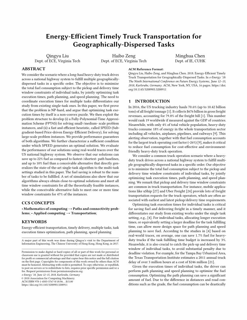
2 MODEL AND PROBLEM FORMULATIONAs illustrated in Fig. 1(a), we study the scenario of one heavy-duty

truck fulfilling multiple tasks in a specific order across a national

Energy-Efficient Timely Truck Transportation for Geographically-Dispersed Tasks e-Energy ’18, June 12–15, 2018, Karlsruhe, Germany

(a) System model: a simple example of a

truck driving in a highway network.

(b) USA highway network partitioned into

22 regions used in our simulations.

Figure 1: A truck timely fulfillsmultiple geo-dispersed tasksin a national highway system to optimize fuel consumption.

highway system. Each task requires to transport given cargos from

a source to a destination satisfying both a source pickup time win-

dow and a destination delivery time window. The objective is to

minimize total incurred fuel consumption. Key notations are sum-

marized in Tab. 5, Appendix 7.1.

2.1 System ModelWe model a national highway network as a directed graph G ,(V ,E) where an edge e ∈ E represents a road segment, and a node

v ∈ V represents an intersection or a connecting point of two

adjacent road segments. Here a road segment is assumed to have

homogeneous grade and environmental conditions like the surface

resistance. We define n , |V | and m , |E |. For each e ∈ E, wedenote De > 0 as its positive distance, r le > 0 (resp. rue ≥ r le )as its positive minimum (resp. maximum) traveling speed, and

cle > 0 (resp. cue ≥ cle ) as its positive minimum (resp. maximum)

fuel consumption.

We consider an eco-routing problem for one heavy-duty truck

across G to fulfill K transportation tasks denoted by ®τ = {τi : i =1, 2, ...,K}. In this paper we have the following two practically

reasonable assumptions for the truck to fulfill the given K tasks ®τ :

(1) the truck must fulfill tasks in a specific given order, namely

the ith task τi must be fulfilled before the jth task τj for any1 ≤ i < j ≤ K , and

(2) the truck cannot transport cargoes belonging to different

tasks simultaneously.

In this paper, each task τi is characterized by a ρi ≥ 0 which is

the weight of its cargoes, a source si ∈ V where the truck can pick

up cargoes, a destination di ∈ V to which cargoes are delivered,

a pickup window sωi defining the allowed time for picking up at

si , and a delivery window dωi representing the allowed time for

delivering at di . We use α(·) (resp. β(·)) to denote the starting time

(resp. ending time) of a window, namely

sωi , [α(sωi ), β(sωi )] , β(sωi ) ≥ α(sωi ) ≥ 0,

dωi , [α(dωi ), β(dωi )] , β(dωi ) ≥ α(dωi ) ≥ 0.

When the truck is expected to pick up τi at source si , earliest ar-rival before α(sωi ) is possible. But the truck cannot leave si untilα(sωi ) when allowed to pick up cargoes. Arrival later than β(sωi )is not permitted since the latest pickup time is missed. The same

assumption holds for the delivery window dωi when the truck is

expected to deliver τi at destination di .

In this paper, we use “deadline" as a constraint imposed on the

maximum travel time to fulfill a task, while “time window" defines

a specific earliest and latest pickup/delivery time at a certain node.

The truck fuel consumption depends on many factors [3]. Similar

to [4], as we consider a specific heavy-duty truck driving over a

specific highway, any environment-specific parameter such as the

gradient is road-segment-dependent and assumed to be fixed for

each specific road segment. Hence given a road segment, the fuel

consumption rate is assumed reasonably to be a function of the

vehicle load, namely the cargo mass of a task, and the vehicle speed.

Same to [4], we neglect the acceleration/deceleration both when

driving inside any road segment (Jensen’s inequality implies driving

at a constant speed is most fuel-economic inside a road segment [4,

Lem. 1]) and when switching between road segments (negligible

compared with the length of real-world road segment). Both load

and speed are key factors in any vehicle fuel consumption models

(see a survey in [3]). According to [3], as estimated by certain

model, the fuel consumption rate can increase by 103% when speed

is increased from 50km/h to 70km/h, and can increase by 27% when

the truck load factor is increased from 0% to 30%.

We define fe (re , ρ) :

[r le , r

ue

]→ R+ as the positive fuel consump-

tion rate for the truck to pass e ∈ E following a constant speed rewith load ρ, which is a function of re given a ρ. Same to the as-

sumption in [4] verified by both physical laws and comprehensive

simulations using real-world data, we assume fe (re , ρ) to be strictly

convex over

[r le , r

ue

]with re given a truck load ρ.

Since each e ∈ E has a fixed distance De , with the fuel rate

fe (re , ρ), we can define a positive fuel consumption function ce (te , ρ)

ce (te , ρ) , te · fe

(Dete, ρ

), (1)

which is the total fuel consumption for the truck to pass e with load

ρ and travel time te . Due to the strict convexity of fe (·), followingthe proof of [4, Lem. 2], it can be proved: (i) ce (te , ρ) is strictly

convex over te ∈

[t le , t

ue

]with te given a truck load ρ, where

t le , De/rue is the minimum travel time and tue , De/r

le is the

maximum travel time, and (ii) there exists a travel time te (ρ) ∈[t le , t

ue

]such that ce (te , ρ) is first strictly decreasing over

[t le , te (ρ)

]and then strictly increasing over

[te (ρ), t

ue], given a specific load ρ.

Hence, to fulfill a specific τi , for any e ∈ E, the possible travel time

in the optimal solution of our problem must belong to the range

of

[t le , te (ρi )

], straightforwardly. Without loss of generality, we

assume ce(te (ρi ), ρi

)≥ cle and ce

(t le , ρi

)≤ cue , since otherwise

we still can figure out the possible travel time range which is a

subset of

[t le , te (ρi )

]in polynomial time, considering the strictly

decreasing property of ce (te , ρi ) over[t le , te (ρi )

].

2.2 Problem FormulationConsidering any two consecutive tasks τi and τi+1 (1 ≤ i ≤ K − 1),

without loss of generality, we assume the delivery node of the ith

task is same as the pickup node of the (i + 1)th task, i.e. di = si+1,

because otherwise we can always add an additional task τK+i withsK+i = di , dK+i = si+1, sωK+i = dωi , dωK+i = sωi+1, ρK+i = 0 to


the task sequence ®τ and in the end |®τ | ≤ 2K . Similarly, we assume

s1 to be the source and dK to be the destination of the whole trip.

By above assumptions, the input tasks ®τ is equivalent to a sequence

®σ of K + 1 nodes for the truck to pass:

®σ = {σi : σ1 = s1,σK+1 = dK ,σi = si = di−1,∀i = 2, 3, ...,K}.

For any node σi , because it is the destination of τi−1 and the source

of τi , it will have two time window constraints, namely the delivery

window dωi−1 and the pickup window sωi . Comparing the two

time window constraints, the earliest allowed leaving time is in fact

max{α(dωi−1),α(sωi )}, denoted by T outi ,

T out1

, α(sω1),Touti , max {α(dωi−1),α(sωi )} , i = 2, 3, ...,K ,

which indicates that the truck cannot leaveσi until he/she can finishboth the delivery of task τi−1 and the pickup of task τi . Similarly,

the latest allowed arrival time, denoted by T ini , is

T inK+1

, β(dωK ),Tini , min {β(dωi−1), β(sωi )} , i = 2, 3, ...,K ,

which indicates that the truck must arrive at the node σi no laterthan both the latest delivery time of task τi−1 and the latest pickup

time of task τi . Overall, all time window constraints associated with

tasks ®τ are now converted equivalently to the earliest leaving time

constraint and latest arrival time constraint for nodes in ®σ .In this paper there are two different kinds of design variables:

binary variable xei defining a path from σi to σi+1 to fulfill τi ,

xei =

{1, e ∈ E is on the path to fulfill the task τi ;0, otherwise,

and non-negative variable tei representing the specific travel time

for the truck to pass edge e to fulfill the task τi .

By vectoring variables as ®xi , {xei : e ∈ E} and ®ti , {tei : e ∈ E},our problem Timely tRansportation for Energy-efficient trucKing,

denoted by TREK, can be formulated as

min

®xi ∈Xi , ®ti ∈Ti

K∑i=1

∑e ∈E

xei · ce (tei , ρi ) (2a)

s.t. ai = max

{ai−1,T

outi

}+

∑e ∈E

xei tei ≤ T in

i+1,

a0 = 0,∀i = 1, 2, ...,K , (2b)

where set Xi defines one path from σi to σi+1,

Xi ,{®xi : xei ∈ {0, 1},∀e ∈ E, and∑

e ∈out(v)xei −

∑e ∈in(v)

xei = 1{v=σi } − 1{v=σi+1 },∀v ∈ V},

where 1{·} is the indicator function, in(v) , {(u,v) : (u,v) ∈ E} is

the set of incoming edges of node v ∈ V , out(v) , {(v,u) : (v,u) ∈E} is the set of outgoing edges of node v ∈ V . Set Ti defines thepossible road travel time,

Ti ,{®ti : t le ≤ tei ≤ te (ρi ),∀e ∈ E

}.

In formulation (2), ai is the exact arrival time at σi+1, which

should be no later than the latest allowed arrival time T ini+1

. The

formula max{ai−1,Touti } guarantees that the truck cannot leave σi

immediately if he/she arrives at σi before the earliest allowed leav-

ing time T outi . Objective (2a) minimizes the total fuel consumption

of the whole trip fulfilling task sequence ®τ .

Table 2: An example illustrating our problem TREK basedon Fig. 1(a), assuming t le = tue = 1 and cle = c

ue for any e ∈ E.

e (1, 2) (2, 3) (1, 3) (3, 4) (4, 5) (3, 5) (1, 5)

ce 1 1 3 1 1 4 8

τi τ1 : 1 → 3 τ2 : 3 → 5

sωi [0, 2] [0, 3]

dωi [0, 2] [0, 3]

In the paper we denote a solution to our problem TREK as

p = p1 ∪ p2 ∪ ... ∪ pK ,

which is a path from σ1 to σK+1 passing all σi ∈ ®σ , with each pibeing a simple path from σi to σi+1, and each edge e ∈ pi assigned

a specific travel time tei ∈ [t le , te (ρi )].An example of TREK is introduced in Tab. 2. The optimal solution

that minimizes the total cost to timely fulfill the two tasks is to

follow the path (1, 3, 4, 5) with the optimal cost to be OPT = 5.

2.3 Challenge and NP-hardnessIntuitively, TREK is hard because (i) path planning and speed plan-

ning are coupled with each other and should be tackled simultane-

ously, and (ii) more importantly, it requires to optimize execution

times for individual tasks jointly such that total cost can be min-

imized, which a non-convex puzzle by itself as illustrated latter

using a simple example. Such an optimization on task execution

times differentiates our work from existing single-task ones (e.g.

the one from [4]) where no execution times optimization will be

involved when they are simply generalized to handle our problem

in the multiple tasks setting.

Suppose we denoteCi (Ti ) as the optimal cost to fulfill the single

task τi with travel time bounded above by a deadline Ti . Thenour problem TREK can also be formulated easily as following with

execution times Ti allocated to τi :

min


K∑i=1

Ci (Ti ) (3a)

s.t. ai = max

{ai−1,T

outi

}+Ti ≤ T in

i+1,

a0 = 0,∀i = 1, 2, ...,K , (3b)∑e ∈E

xei tei ≤ Ti ,∀i = 1, 2, ...,K , (3c)

where we try to achieve the optimal task execution times allocation

results Ti , i = 1, 2, ...,K with all time window constraints satisfied.

If we can find the optimal Ti , i = 1, 2, ...K for all individual tasks,

we can run existing single-task algorithm (e.g. the one proposed

by [4]) K times independently and obtain the solution in the end.

However, we argue that it is hard to optimize the execution times

for individual times, due to the non-convexity of the function Ci (·).Consider network in Fig. 1(a) where there is only one task with

source 1 and destination 5. Edge travel time and cost are the same

as defined in Tab. 2. It is clear that in Fig. 1(a) there are 5 different

paths from node 1 to node 5. By enumerating all those 5 paths

with associated path cost and path travel time, we have C(T ) = 4

when T = 4 following the path (1, 2, 3, 4, 5), C(T ) = 5 when T = 3

following the path (1, 3, 4, 5), C(T ) = 7 when T = 2 following the


path (1, 3, 5), and C(T ) = 8 when T = 1 following the path (1, 5).

Clearly, the optimal cost C(T ) is neither convex nor concave in T .The following theorem shows that TREK is NP-hard, which is

not surprising since its special cases RSP [7, 16] and PASO [4] are

both NP-hard.

Theorem 2.1. TREK is NP-hard.

Proof. Refer to Appendix 7.3. �

In this paper we develop an FPTAS and a heuristic to solve TREK.FPTAS optimizes the task execution times by intelligently enumer-

ating possible results without incurring excessive complexity, and

then selecting the best. And heuristic optimizes the task execution

times by allocating deadlines for individual tasks jointly and itera-

tively towards the optimal based on dual sub-gradient information.

3 AN FPTAS FOR TREKIn this section we develop an FPTAS for TREK, based on Dynamic

Programming (DP) and an extension of the FPTASes proposed

by [4, 16] solving problem RSP and PASO, respectively. Our FPTASsolves the NP-hard problem TREK with an approximation ratio of

(1 + ϵ) in fully polynomial time, for any ϵ > 0.

3.1 Dynamic Programming for TREKWe observe that our problem TREK satisfies Bellman’s principle

of optimality, and hence can be solved by DP. Specifically, we di-vide problem TREK to two sub-problems: (i) we first obtain all

possible solutions to independently fulfill the single task τi for alli = 1, 2, ...,K , by enumerating either all travel-time-bounded min-

cost path or all cost-bounded min-travel-time path, and (ii) we then

select exactly one solution per task, with the combined solution

satisfying all time window constraints and minimizing the total

cost. Both sub-problems can be handled by DP.We need discrete (e.g., integral) edge travel time or cost in order

to use DP to solve TREK. If we require integral edge travel time,

the Bellman’s equation for sub-problem 1 is simply the equation

in (12), Appendix 7.2, and the Bellman’s equation for sub-problem

2 is the equation in (14), Appendix 7.2. If we require integral edge

cost instead of integral travel time, the Bellman’s equation for sub-

problem 1 is the equation in (13), Appendix 7.2, and the Bellman’s

equation for sub-problem 2 is the equation in (15), Appendix 7.2.

Due to the space limitation, we put algorithmic details of proposed

DP approach in Appendix 7.2. Overall, we can useDP to solve TREK,and optimal solution is guaranteed if either all edge travel time or

all edge cost are required to be integers. However, the DP approach

suffers from a pseudo-polynomial time complexity in theory.

A nature idea to solve TREK in polynomial time is to follow our

DP with rounding and scaling on edge travel time (for Bellman’s

equation in (12) and in (14)) or edge cost (for Bellman’s equation

in (13) and in (15)). Considering that in our problem any violation

of time window constraints is not allowed, clearly it is better to

discretize, quantize and approximate edge cost such that precise

edge travel time information can be kept. In this paper, we extend

the FPTASes proposed by [4, 16] both of which use similar ideas of

edge cost quantization, and design an FPTAS for TREK.

3.2 A Test ProcedureThe essence of our FPTAS is a test procedure which approximately

compares the optimal cost of TREK to an arbitrary input, with

details introduced in Algorithm 1. The structure of Algorithm 1 is

the same as the above DP approach, except that edge cost has been

quantized to guarantee a polynomial time complexity: the loop of

line 8 is equivalent to the Bellman’s equation in (13) handling the

sub-problem 1, and the loop of line 13 is equivalent to the Bellman’s

equation in (15) solving the sub-problem 2.

Algorithm 1 Test(G, ®σ ,L,U , ϵ)

1: procedure2: S = Lϵ

K (n+1), U =

⌊US⌋+ K(n + 1), ptest = NULL

3: for ∀i = 1, 2, ...,K ,∀e ∈ E,∀c = 1, 2, ..., U do4: cle = ⌈ce (te (ρi ), ρi )/S⌉, c

ue = ⌈ce (t

le , ρi )/S⌉

5: tei (c) =

t le , if c = cuec−1

e (cS, ρi ), if cle ≤ c < cue+∞, otherwise

6: Set Ti (v, 0) = +∞,∀i = 1, 2, ...,K ,∀v , σi : v ∈ V7: Set Ti (σi , 0) = 0,∀i = 1, 2, ...,K8: for ∀i = 1, 2, ...,K ,∀c = 1, 2, ..., U ,∀v ∈ V do9: Ti (v, c) = Ti (v, c − 1)

10: for ∀e = (u,v) ∈ E,∀c = 1, 2, ..., c do11: Ti (v, c) = min

{Ti (v, c),Ti (u, c − c) + tei (c)

}12: Set T(σ1, c) = 0,∀c = 0, 1, ..., U13: for ∀i = 2, 3, ...,K + 1,∀c = 1, 2, ..., U do14: T(σi , c) = T(σi , c − 1)

15: for ∀c = 1, 2, ..., c do16: T = max

{T(σi−1, c − c),T out

i−1

}+ Ti−1(σi , c)

17: T =

{T , if T ≤ T in

i ;

+∞, otherwise,

18: T(σi , c) = min {T (σi , c),T }

19: c∗ is the minimal c ∈ {1, 2, ..., U } : T(σK+1, c) ≤ T inK+1

20: If c∗ exists, ptest is defined by T(σK+1, c∗)

21: return ptest

To be specific, as proved in our Lem. 7.1, Appendix 7.4, in Al-

gorithm 1 we first quantize edge cost c to be c where c = ⌈c/S⌉in the loop of line 3. As a result, a polynomial time complexity

can be guaranteed for Algorithm 1 as described in our Lem. 7.5,

Appendix 7.8. Moreover, such a quantization technique can provide

bounded performance difference comparing the quantized cost to

the precise cost before quantization, which is introduced in our

Lem. 7.2, Appendix 7.5. Algorithm 1 is critical for our FPTAS becauseit can approximately compare the optimal cost of TREK, i.e. OPT,to an arbitrary inputU , in the sense that if it returns a non-empty

solution, it must hold that OPT ≤ U + Lϵ (Lem. 7.3, Appendix 7.6);

otherwise, we must have OPT > U (Lem. 7.4, Appendix 7.7).

We remark that the returned solution of Algorithm 1 must meet

all the time window constraints, which is guaranteed by the Bell-

man’s equation in (15) in the loop of line 13.


Algorithm 2 FPTAS-TREK(G, ®σ ,LB,UB, ϵ)

1: procedure2: pfptas = NULL,BL = LB,BU = ⌈UB/2⌉

3: while BU /BL > 2 do4: B =

√BL · BU

5: if Test(G, ®σ ,B,B, 1) = NULL then6: BL = B7: else8: BU = B

9: pfptas = Test(G, ®σ ,BL , 2BU , ϵ)10: return pfptas

3.3 Proposed FPTASWith our test procedure of Algorithm 1, we follow the same struc-

ture of the FPTAS proposed by [16] for solving RSP, and design an

FPTAS in Algorithm 2 for our problem TREK in this section.

With an initial lower bound LB ≤ OPT and an initial upper

boundUB ≥ OPT, our FPTAS first narrows down the gap BU /BLwhere 2BU (resp. BL ) is always a valid upper (resp. lower) bound ofOPT (proved in our Lem 7.6, Appendix 7.9) using a binary search

scheme. When the gap is below 2, the (1 + ϵ)-approximate solution

is achieved by calling test procedure Test(G, ®σ ,B, 2B, ϵ) in line 9.

By the following two theorems, Algorithm 2 is proved to be

an FPTAS for TREK, providing a (1 + ϵ)-approximation ratio in

polynomial time with all problem input and 1/ϵ .

Theorem 3.1. Given a lower bound LB and an upper boundUBof the optimal cost OPT, and assume that the feasible set of TREK isnot empty, then Algorithm 2 will return a non-empty solution pfptasthat satisfies

c(pfptas

)≤ (1 + ϵ)OPT,

where c(pfptas

)represents the total cost of our solution pfptas.

Proof. Refer to Appendix 7.10 due to the space limitation. �

Theorem 3.2. Algorithm 2 has a time complexity of

O

(mK3n3

(log log

UB

LB+

(1 +

1

ϵ

)2

)).

Proof. A direct result following Lem. 7.5. �

To initialize our FPTAS, we need to first obtain a lower bound LBand an upper bound UB for the optimal cost OPT. It is straightfor-ward that LB ≥ K · mine ∈E c

le and UB ≤ Kn · maxe ∈E c

ue , leading

to that UB/LB ≤ n · maxe ∈E cue /mine ∈E c

le . Considering the time

complexity described in Thm. 3.2, clearly that our proposed Algo-

rithm 2 has a polynomial time complexity with all problem input

{n,m,K , cle , cue : ∀e ∈ E} and 1/ϵ . Since log log

U BLB is relative small

as compared tomK3n3/ϵ2, we can roughly represent the time com-

plexity of our FPTAS as O(mK3n3/ϵ2).

In summary, the proposed FPTAS achieves an approximation

ratio of (1 + ϵ) for any ϵ > 0 with fully polynomial time complex-

ity. This makes it suitable for solving small-/medium- scale TREKinstances. For large-scale instances such as those over the US na-

tional highway networks, however, we observe empirically that

the FPTAS may take an excessive amount of time to generate its

solution. This motivates us further to design a fast and efficient

alternative for solving large-scale TREK instances.

4 SPEED: A FAST AND EFFICIENT HEURISTICIn this section, we develop an efficient dual-based algorithm, named

SPEED (in short for Sub-gradient-based Price-driven Energy-Efficient

Delivery), for solving large-scale TREK instances. SPEED iteratively

allocates execution times for individual tasks towards the optimal,

by following the sub-gradient of the Lagrangian dual relaxation.

We derive a performance bound between the solution of SPEEDand the optimal solution, and we further characterize a condition

under which SPEED generates an optimal solution.

4.1 A New Problem Formulation of TREKIn this section, we first reformulate TREK and give a new formula-

tion in (4), which is characterized by the travel time upper bound

constraint imposed on any consecutive tasks {τk ,τk+1, ...,τr ,∀r =

1, 2, ...,K ,∀k = 1, 2, ..., r }:

min


K∑i=1

∑e ∈E

xei · ce (tei , ρi ) (4a)

s.t.

r∑j=k

∑e ∈E

xej tej ≤ T in

r+1−T out

k ,

∀r = 1, 2, ...,K ,∀k = 1, 2, ..., r , (4b)

Theorem 4.1. The problems in (2) and (4) are equivalent in thatthey share the same objective function and the constraint sets areequivalent.


The deadline constraints in (4b) require that given any r and anyk ≤ r , the total travel time from σk to σr+1, i.e., the aggregated

execution times of τk ,τk+1, ...τr , should be bounded above byT

inr+1

−

T outk which is the gap between the latest arrival time of σr+1 and

the earliest leaving time of σk . While the number of constraints

in the formulation in (4) increases from K to K2as compared to

the formulation in (2), the new formulation in (4) is critical for

developing our sub-gradient based algorithm SPEED.

4.2 The Dual Problem of TREKWe relax the deadline constraints in (4b) to the objective function

by introducing a Lagrangian dual variable λrk for each (k, r ) pairand obtain the following Lagrangian function

L(®x , ®t , ®λ

),

K∑r=1

r∑k=1

λrk ·©«

r∑j=k

∑e ∈E

xej tej −T in

r+1+T out

kª®¬

+

K∑i=1

∑e ∈E

xei · ce(tei , ρi

).

The specific dual variable λrk in the Lagrangian function is only

associated with the travel time of tasks from τk to τr . Now given

a specific task τi , we look at all the dual variables associated with

it. To this end we observe that λrk is associated with τi if and only


if k ≤ i ≤ r , and the set of the dual variables associated with τi isthus {λrk : ∀k ≤ i,∀r ≥ i}. We have

K∑r=1

r∑k=1

λrk

r∑j=k

∑e ∈E

xej tej =

K∑i=1

∑e ∈E

xei tei

K∑r=i

i∑k=1

λrk , (5)

since both sides of the equation in (5) are the sum of the dual

variable times the task fulfilling time over all correlative tasks and

dual variables. Using the equation in (5), our Lagrangian function

can be presented as follows

L(®x , ®t , ®λ

)=

K∑i=1

∑e ∈E

xei ·

[ce (t

ei , ρi ) + t

ei

K∑r=i

i∑k=1

λrk

]−

K∑r=1

r∑k=1

λrk

(T inr+1

−T outk

).

We define µi as the sum of all the dual variables associated with

task τi in the following

µi ,K∑r=i

i∑k=1

λrk , (6)

then our Lagrangian function is

L(®x , ®t , ®λ

)=

K∑i=1

∑e ∈E

xei ·[ce (t

ei , ρi ) + t

ei µi

]−

K∑r=1

r∑k=1

λrk

(T inr+1

−T outk

).

The dual problem of TREK is

max

®λ≥0

D(®λ)

: D(®λ), min

®x, ®tL

(®x , ®t , ®λ

),

where D(®λ)is the dual function. The following theorem gives an

explicit formula for D(®λ).

Theorem 4.2.

D(®λ)= −

K∑r=1

r∑k=1

λrk

(T inr+1

−T outk

)+

K∑i=1

∑e ∈p(µi )

wei (µi ),

wherewei (µi ) , ce

(tei (µi ), ρi

)+ µi t

ei (µi ), (7)

withtei (µi ) , arg min

t le ≤t ei ≤te (ρi )

(ce (t

ei , ρi ) + µi t

ei). (8)


In the above Thm. 4.2, tei (µi ) is the optimal travel time that

minimizes the edge cost but with a price µi imposed on the edge

travel time given specific µi . Since we have assumed ce(tei , ρi

)to be strictly convex and strictly decreasing over tei ∈

[t le , te (ρi )

],

tei (µi ) is well defined. Hence,wei (µi ) is the optimal penalized edge

cost including the fuel consumption cost and the travel time cost

given the price µi , and we denote the minimal penalized cost path

from σi to σi+1 as p(µi ).

According to Thm. 4.2, given a set of dual variables®λ, we can

obtain the value of the dual function D(®λ)by solving K shortest

path problems, each of which minimizes the penalized cost for a

specific task. One can solve these shortest path problems by using

standard algorithms, e.g., the Dijkstra’s algorithm [5]. Therefore,

we can design an efficient heuristic for TREK by iteratively update

dual variables®λ to minimize the duality gap.

4.3 The SPEED AlgorithmWe further define δ (µi ) as the travel time of the path p(µi ):

δ (µi ) ,∑

e ∈p(µi )

tei (µi ). (9)

Similar to [4, Thm.3], a key observation of δ (µi ) is presented in

the following theorem.

Theorem 4.3. δ (µi ) is non-increasing in µi ∈ [0,+∞) for anyi = 1, 2, ...,K .

Proof. The proof is similar to that of [4, Thm.3] and is skipped.

�

In the next, we introduce a set of complementary-slackness-like

conditions for®λ and δ (·). If the conditions are satisfied, then we

can derive an optimal solution to TREK.

Theorem 4.4. Suppose the dual variable {λrk : ∀r = 1, 2, ...,K ,∀k =1, 2, ..., r }, the {µi ,∀i = 1, 2, ..,K} computed in (6), and the {δ (µi ),∀i =1, 2, ...,K}) computed in (9) satisfy thatT out

k −T inr+1+

r∑j=k

δ (µ j )

+

λrk

= 0,

∀r = 1, 2, ...,K ,∀k = 1, 2, ..., r , (10)

where function [f ]+д is defined as

[f ]+д =

{max{ f , 0}, if д ≤ 0;f , otherwise.

Then each p(µi ) specifies a path for fulfilling task τi with the assignedtravel time tei (µi ) for each edge e ∈ p(µi ), and this solution mustbe the optimal solution to our problem TREK. The starting time andending time of tasks {τi , i = 1, 2...,K} can be computed following thetime window constraints in (2b) from τ1 to τK iteratively one by one.


SPEED uses a sub-gradient based heuristic scheme inAlgorithm 3

to iteratively update dual variables towards satisfying conditions

in (10):

Ûλrk = ϕ(λrk ) ·

T outk −T in

r+1+

r∑j=k

δ (µ j )

+

λrk

,

∀r = 1, 2, ...,K ,∀k = 1, 2, ..., r , (11)

where ϕ(λrk ) is a positive step size to update λrk . The step is positive

instead of negative due to Thm. 4.3. The following theorem shows

that SPEED always gives a feasible solution for any theoretically-

feasible TREK instances. We further present the performance bound

between SPEED solution and the optimal in the following theorem.


Algorithm 3 SPEED(G, ®σ )

1: procedure2: Set ite=1, λrk =

Ûλrk = λmax,∀r = 1, 2, ...,K ,k = 1, 2, ..., r .

3: while ∃ r ,k :

�� Ûλrk �� > tol and ite ≤ ITE do4: for i = 1, 2, ...,K do5: Set µi according to equality (6)

6: Obtain tei (µi ),∀e ∈ E according to equality (8)

7: Setwei (µi ),∀e ∈ E according to equality (7)

8: Get the σi − σi+1 shortest path p(µi ) withwei (µi )

9: ph = {p(µi ) : i = 1, 2, ...,K}, ite = ite + 1

10: SetÛλrk ,∀r ,∀k according to equality (11)

11: Set λrk = λrk +Ûλrk ,∀r = 1, 2, ...,K ,∀k = 1, 2, ..., r

12: if Ûλrk = 0,∀r = 1, 2, ...,K ,k = 1, 2, ..., r then13: return p = ph14: if ph is feasible and c(ph ) < c(p) then15: p = ph16: if ph is not feasible then17:

Ûλrk = λmax,∀r = 1, 2, ...,K ,∀k = 1, 2, ..., r

18: return p

Theorem 4.5. For any theoretically-feasible TREK instance, Al-gorithm 3 returns a feasible solution p. The optimality gap betweenthe cost of p, namely c(p), and the optimal cost, namely OPT, mustbe bounded above as follows:

c(p)−OPT ≤

{0, case 1;

K2 · max∀r,k�� Ûλrk �� · max∀r,k

{¯λrk/ϕ(

¯λrk )}, case 2,

where case 1 is for p returned in line 13, case 2 is for p returned inline 18. { ¯λrk ,∀r = 1, ...,K ,∀k = 1, ..., r } is the set of dual variablescorresponding to p.


From Thm. 4.5, it is clear that if Algorithm 3 is terminated in the

line 13, the obtained solution is optimal. Another direct application

of our Thm. 4.5 is to obtain a high-quality lower bound of the opti-

mal cost in simulations, and thus efficiently evaluate performances

of different algorithms for TREK. Practically, one critical applicationof Thm. 4.5 is that it can help us terminate Algorithm 3 and achieve

a solution meeting all time window constraints, once the optimality

gap of the achieved solution is below a user-defined tolerance, hence

leading to much shorter algorithm running time without waiting

for the convergence whenÛλrk = 0,∀r = 1, ...,K ,∀k = 1, ..., r .

Overall in this section, we develop an efficient heuristic SPEED(Algorithm 3) for TREK, by iteratively updating dual variables

(equality (11)) and then solving the dual function (Thm. 4.2), in

order to minimize the duality gap (Thm. 4.4). Hence SPEED can

allocate task execution times efficiently using the feedback of dual

sub-gradient information. We characterize a performance bound of

the solution of SPEED, and moreover, give conditions under which

the solution of SPEED is guaranteed to be optimal (Thm. 4.5).

Table 3: Performance comparison of FPTAS (F) and SPEED(S), where the unit of fuel consumption is gallon and the unitof the running time is second. LB is a lower bound for theoptimal solution and obtained from Thm. 4.5.

Problem Input Fuel-Cost Run-Time(σ1,σ2,σ3,T

in2,T in

3) ϵ LB S F S F

(2, 1, 6, 7, 12) 0.1 123.45 125.55 125.9 44 5760

(14, 17, 18, 7, 12) 0.1 135.18 137.88 N/A 65 N/A

5 PERFORMANCE EVALUATIONWe use real-world traces to evaluate our FPTAS and SPEED, bycomparing them with fastest-/shortest- path baselines and a con-

ceivable alternative which directly generalizes the state-of-the-art

single-task algorithm from [4] to the multi-task settings studied in

this paper. We implement all algorithms using C++ and run them

on a laptop with 4-core Intel Core-i5-4200M (2.50 GHz) processor

and 16 GB memory, running 64-bit Ubuntu 16.04 LTS, for compari-

son. We use the SNAP graph structure [15] and construct the U.S.

national highway system (NHS) from the Clinched Highway Map-

ping Project [22] consisting of 84504 nodes and 178238 directed

edges. Road grade is obtained from the elevations of each node

provided by the Elevation Point Query Service [26] from the U.S.

Geological Survey. The maximum speed rue is set to be the histor-

ical average speed by collecting real-time speed data from HEREmap [8] for 2 weeks, and the minimum speed r le is manually set to

be r le = min{30, rue }. We use ADVISOR simulator [17] to collect fuel

consumption rate data with driving speed (from 10mph to 70mph

with a step of 0.2mph) for different road grade (from −10.0◦ to 10.0◦

with a step of 0.1◦) and truck load (empty load, half load, and full

load) for a class 8 heavy truck of Kenworth T800 [11]. Then we use

the curve fitting toolbox in MATLAB to learn the fuel consumption

rate function fe (re , ρ) modeled as a 3-order polynomial function

with speed given specific road grade and truck load.

Same to [4], the NHS graph is preprocessed first: (i) the graph is

cut to the “eastern" part, (ii) non-intersection roads with the same

grade level are merged into a single road segment, and (iii) the

“eastern" U.S. is divided into 22 regions (see Fig. 1(b)), where the node

nearest to each region’s center is used as the source and destination

nodes in the experiment. After preprocessing, the number of nodes

is 38213 and the number of edges is 82781.

In our simulations, we set all earliest leaving time constraints

to be 0, namely T outi = 0,∀i = 1, ...,K . As for the experimental

parameters of our SPEED in Algorithm 3, we fix ϕ(·) to be 0.1 for

all dual variables, tol to be 0.01 and ITE to be 50.

5.1 Performance Comparison of FPTAS andSPEED

We consider the setting where the truck fulfills two tasks both with

full load. Results for two instances are shown in Tab. 3. In both

instances, the solutions of SPEED are close-to-optimal, with the

optimality gap being upper bounded by 3 gallons (2% of the optimal

cost). FPTAS can only handle the smallest instance (first instance

with n = 1518 andm = 3274) for ϵ = 0.1. Compared with SPEED,FPTAS incurs much longer (100×) running time for the first instance.

For the second instance with n = 6187 andm = 13708 where source


and destination of each task are located in neighboring regions,

FPTAS fails to output a solution even after running it for 12 hours.

5.2 Performance Comparison of SPEED andOther Alternatives

In this section we compare SPEED with two baselines and a con-

ceivable alternative approach:

(1) A fastest-path-based approach without task execution times

optimization: the travel speed re for each e ∈ E is fixed

as re = rue , and each task τi is fulfilled using the path with

minimal travel time from its source σi to its destination σi+1.

(2) A shortest-path-based approachwithout task execution times

optimization: the travel speed re for each e ∈ E is fixed as

re = rue , and each τi is fulfilled using the path with minimal

travel distance from its source σi to its destination σi+1.

(3) A PASO-based approach with greedy task execution times

allocation: we greedily allocate deadlines as large as possi-

ble for individual tasks from the first task to the last task

iteratively one by one. To be specific in the ith iteration, we

run the heuristic proposed by [4] to solve problem PASOfor the single task τi , minimizing the fuel consumption from

σi to σi+1 with a deadline of T ini+1

− max{T outi ,ai−1}, where

ai−1 is defined in formula (2), which is the truck arrival time

at σi and can be achieved since we have solved the PASOproblems for tasks {τ1,τ2, ...,τi−1} before the ith iteration.

We consider two tasks with the first task from 1 to 9 and the

second task from 9 to 22, assuming full load for both tasks and

T in2= 40,T in

3= 65. This TREK instance is denoted as a tuple of

(σ1,σ2,σ3,Tin2,T in

3) = (1, 9, 22, 40, 65). We remark that the instance

(1, 9, 22, 40, 65) is representative because (i) both tasks are heavy-

duty (both tasks are assumed with a full load requirement) and

long-haul (both tasks require the truck to travel across US), and

(ii) the latest arrival time constraints T in2

and T in3

are larger than

the minimal task execution times, allowing a large design space for

task execution times optimization for saving fuel.

Detailed simulation results are shown in Tab. 4. In the table we

also present the increment (%) of the travel time, travel distance

and fuel consumption for the four solutions compared with the

respective optimums. As shown by Tab. 4, both the fastest solution

and the shortest solution consumes ~30% more fuel than SPEED.The PASO solution saves fuel for the individual task τ1 in the cost of

a larger travel time compared with SPEED. However, its solution is

far from optimal, due to its greedy and non-optimal task execution

times allocation (~40 hours for τ1 and ~25 hours for τ2). The solution

of SPEED is close-to-optimal and saves 10% fuel compared with the

PASO solution, with a close-to-optimal execution time allocated

for each task (~29 hours for τ1 and ~36 hours for τ2).

We already know our problem TREK requires a joint optimization

on task execution times, path planning, and speed planning. Tab. 4

presents the impacts of the three optimization aspects on saving

fuel, by comparing SPEED with the non-optimal baselines and

the PASO alternative. From Tab. 4, the travel distance of the four

algorithms are similar, in spite of the various travel time and fuel

consumption. This highlights the importance of exploring speed

planning and task execution times optimization, in addition to path

planning, in reducing fuel consumption.

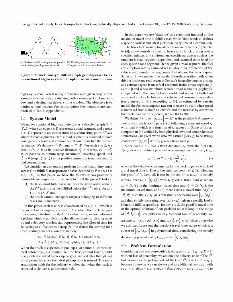
(a) (1, 22, 9, T in2, 65): T in

2is enumer-

ated from 30 to 40 with a unit step.

(b) (1, 22, 9, 40, T in3): T in

3is enumer-

ated from 66 to 85 with a unit step.

Figure 2: Impact of the latest arrival timeT in2

andT in3

on thetotal fuel consumption performance.

5.3 Impact of Time Windows on the CostFor instances of two tasks each with a full load, we respectively

estimate the effect of the two latest arrival time constraintsT in2

and

T in3

on the performance of different algorithms. For the instance

of τ1 from 1 to 22 and τ2 from 22 to 9, we first fix T in3

to be 65 and

evaluate effect from T in2. Results are shown in Fig. 2(a). The fastest-

path-based solution performs almost same as the the shortest-path-

based solution, and is independent to T in2. For T in

2≤ 32, both PASO

and SPEED obtain near-optimal performances, because the greedy

task execution times allocation (T in2

hours for τ1 and 65−T in2

hours

for τ3) is close-to-optimal. For T in2

∈ (32, 40], SPEED guarantees

a close-to-optimal solution and greatly outperforms PASO, sincethe greedy allocation in PASO is far from optimal (the optimal

travel time for τ1 is strictly smaller than T in2). Moreover, PASO

fails to obtain a feasible solution for T in2

≥ 41, since following the

greedy allocation strategy, τ2 is assigned a deadline of 65−T in2< 24

which is smaller than the minimal travel time (24.55) from σ2 to σ3.

Meanwhile, SPEED always provides near-optimal feasible solutions.

We then fixT in2

to be 40 and evaluate the effect fromT in3

with the

results presented in Fig. 2(b). For T in3

∈ [65, 79], SPEED allocates

execution times for tasks properly (a travel time strictly smaller

than 40 hours for τ1 and remaining for τ2), while PASO cannot (it

always assign ~40 hours to τ1 andTin3−40 hours to τ2). ForT

in3

≥ 80,

both PASO and SPEED allocate execution times for tasks properly.

For the instance (1, 22, 9,T in2, 65), since the minimal execution

time of τ1 (resp. τ2) is 24.84 (resp. 24.55), clearly that the feasibility

region of T in2

where our TREK is solvable is T in2

∈ [24.84, 65]. Com-

pared with SPEED which always gives near-optimal solutions for

all solvable problem instances, PASOmay fail to generate a feasible

solution, because that the greedy task execution times allocation

scheme fails to allocate a feasible task execution time for the task

τ2 when T in2> 65 − 24.55.

We further estimate the number of solvable problem instances

for PASO with 100 random simulations. In each simulation, we

randomly select σ1,σ2 and σ3, assuming full load for both tasks.

Suppose the minimal execution time for τ1 is t∗1(resp. t∗

2for τ2),

we randomly select an increment x% ∈ [10%, 100%] and fix T in3

to be T in3= (t∗

1+ t∗

2) · (1 + x%). For this simulation characterized

by (σ1,σ2,σ3,Tin2,T in

3) with the feasibility region of T in

2∈ [t∗

1,T in

3],

we run the PASO-based alternative to obtain the maximum time


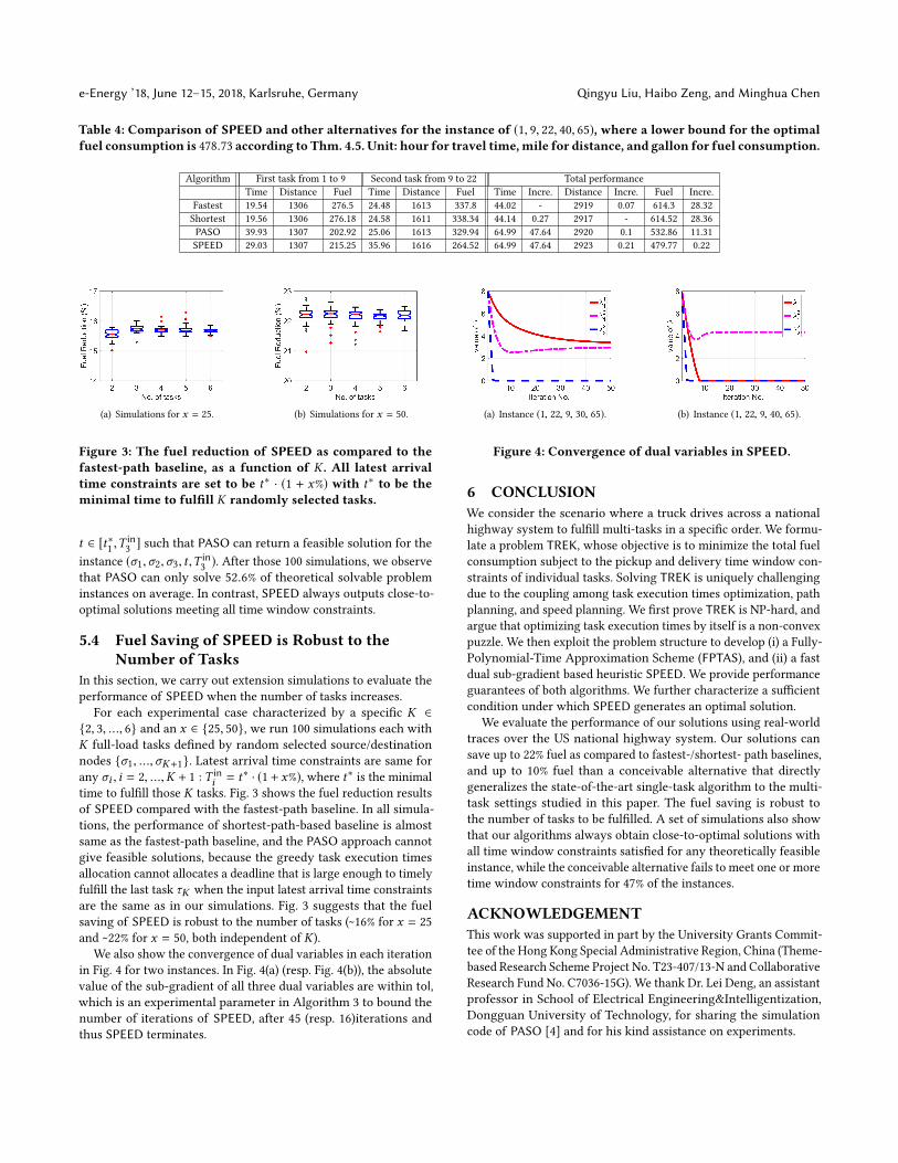
Table 4: Comparison of SPEED and other alternatives for the instance of (1, 9, 22, 40, 65), where a lower bound for the optimalfuel consumption is 478.73 according to Thm. 4.5. Unit: hour for travel time,mile for distance, and gallon for fuel consumption.

Algorithm First task from 1 to 9 Second task from 9 to 22 Total performance

Time Distance Fuel Time Distance Fuel Time Incre. Distance Incre. Fuel Incre.

Fastest 19.54 1306 276.5 24.48 1613 337.8 44.02 - 2919 0.07 614.3 28.32

Shortest 19.56 1306 276.18 24.58 1611 338.34 44.14 0.27 2917 - 614.52 28.36

PASO 39.93 1307 202.92 25.06 1613 329.94 64.99 47.64 2920 0.1 532.86 11.31

SPEED 29.03 1307 215.25 35.96 1616 264.52 64.99 47.64 2923 0.21 479.77 0.22

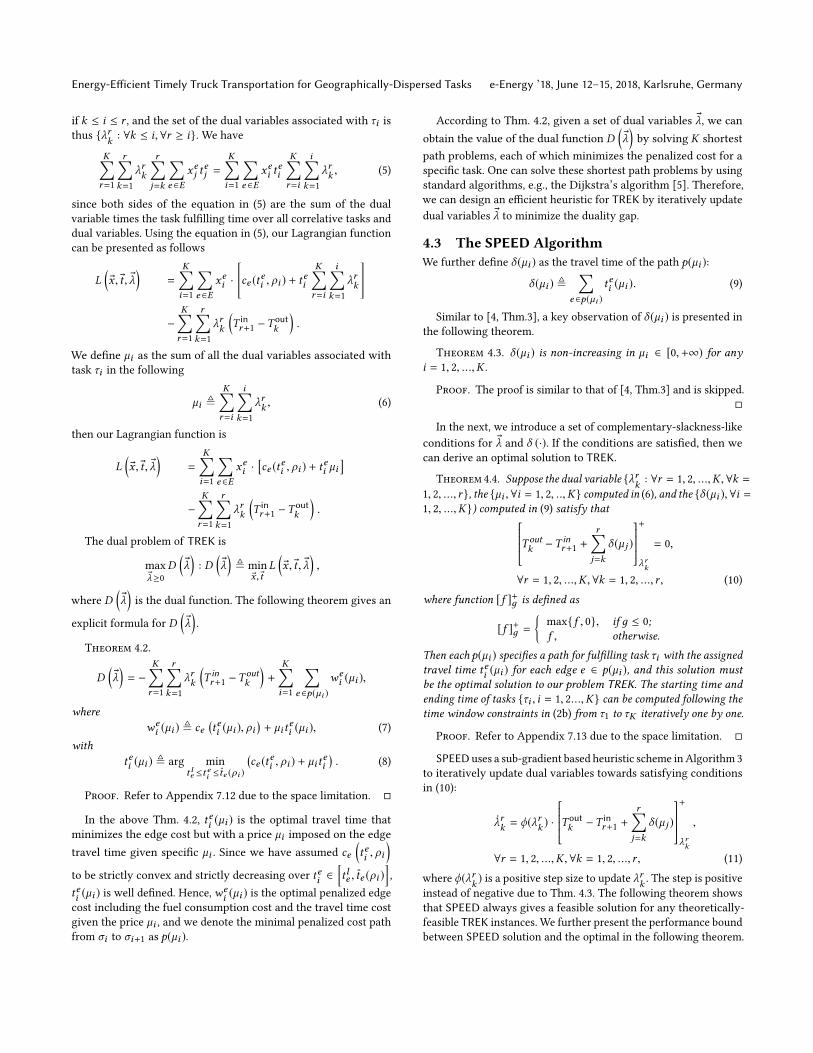
(a) Simulations for x = 25. (b) Simulations for x = 50.

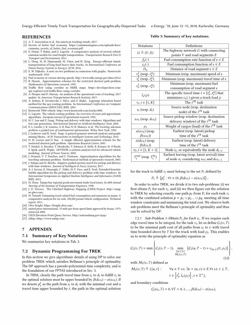
Figure 3: The fuel reduction of SPEED as compared to thefastest-path baseline, as a function of K . All latest arrivaltime constraints are set to be t∗ · (1 + x%) with t∗ to be theminimal time to fulfill K randomly selected tasks.

t ∈ [t∗1,T in

3] such that PASO can return a feasible solution for the

instance (σ1,σ2,σ3, t ,Tin3). After those 100 simulations, we observe

that PASO can only solve 52.6% of theoretical solvable problem

instances on average. In contrast, SPEED always outputs close-to-

optimal solutions meeting all time window constraints.

5.4 Fuel Saving of SPEED is Robust to theNumber of Tasks

In this section, we carry out extension simulations to evaluate the

performance of SPEED when the number of tasks increases.

For each experimental case characterized by a specific K ∈

{2, 3, ..., 6} and an x ∈ {25, 50}, we run 100 simulations each with

K full-load tasks defined by random selected source/destination

nodes {σ1, ...,σK+1}. Latest arrival time constraints are same for

any σi , i = 2, ...,K + 1 : T ini = t∗ · (1 + x%), where t∗ is the minimal

time to fulfill those K tasks. Fig. 3 shows the fuel reduction results

of SPEED compared with the fastest-path baseline. In all simula-

tions, the performance of shortest-path-based baseline is almost

same as the fastest-path baseline, and the PASO approach cannot

give feasible solutions, because the greedy task execution times

allocation cannot allocates a deadline that is large enough to timely

fulfill the last task τK when the input latest arrival time constraints

are the same as in our simulations. Fig. 3 suggests that the fuel

saving of SPEED is robust to the number of tasks (~16% for x = 25

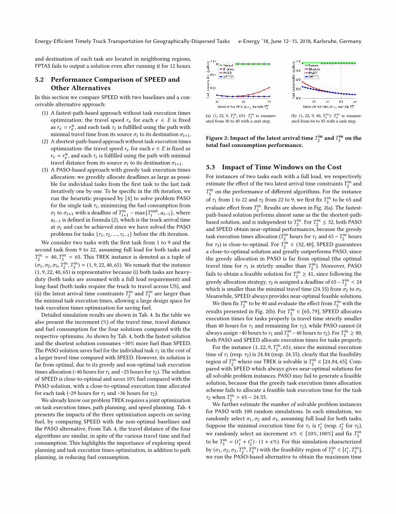
and ~22% for x = 50, both independent of K ).We also show the convergence of dual variables in each iteration

in Fig. 4 for two instances. In Fig. 4(a) (resp. Fig. 4(b)), the absolute

value of the sub-gradient of all three dual variables are within tol,which is an experimental parameter in Algorithm 3 to bound the

number of iterations of SPEED, after 45 (resp. 16)iterations and

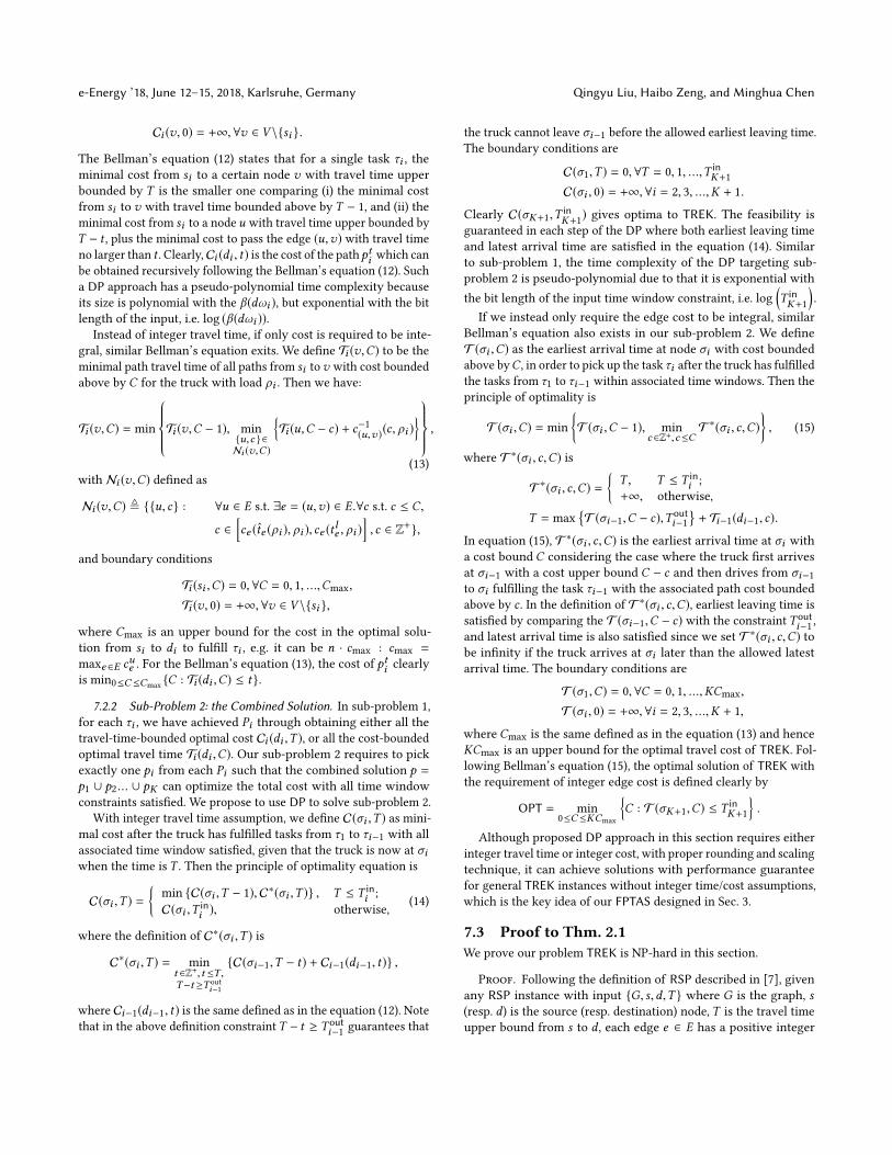
thus SPEED terminates.

(a) Instance (1, 22, 9, 30, 65). (b) Instance (1, 22, 9, 40, 65).

Figure 4: Convergence of dual variables in SPEED.

6 CONCLUSIONWe consider the scenario where a truck drives across a national

highway system to fulfill multi-tasks in a specific order. We formu-

late a problem TREK, whose objective is to minimize the total fuel

consumption subject to the pickup and delivery time window con-

straints of individual tasks. Solving TREK is uniquely challenging

due to the coupling among task execution times optimization, path

planning, and speed planning. We first prove TREK is NP-hard, and

argue that optimizing task execution times by itself is a non-convex

puzzle. We then exploit the problem structure to develop (i) a Fully-

Polynomial-Time Approximation Scheme (FPTAS), and (ii) a fast

dual sub-gradient based heuristic SPEED. We provide performance

guarantees of both algorithms. We further characterize a sufficient

condition under which SPEED generates an optimal solution.

We evaluate the performance of our solutions using real-world

traces over the US national highway system. Our solutions can

save up to 22% fuel as compared to fastest-/shortest- path baselines,

and up to 10% fuel than a conceivable alternative that directly

generalizes the state-of-the-art single-task algorithm to the multi-

task settings studied in this paper. The fuel saving is robust to

the number of tasks to be fulfilled. A set of simulations also show

that our algorithms always obtain close-to-optimal solutions with

all time window constraints satisfied for any theoretically feasible

instance, while the conceivable alternative fails to meet one or more

time window constraints for 47% of the instances.

ACKNOWLEDGEMENTThis work was supported in part by the University Grants Commit-

tee of the Hong Kong Special Administrative Region, China (Theme-

based Research Scheme Project No. T23-407/13-N and Collaborative

Research Fund No. C7036-15G). We thank Dr. Lei Deng, an assistant

professor in School of Electrical Engineering&Intelligentization,

Dongguan University of Technology, for sharing the simulation

code of PASO [4] and for his kind assistance on experiments.


REFERENCES[1] A. T. Association et al. Ata american trucking trends, 2017.

[2] Secrets of better fuel economy. https://cumminsengines.com/uploads/docs/

cummins_secrets_of_better_fuel_economy.pdf.

[3] E. Demir, T. Bekta, and G. Laporte. A comparative analysis of several vehicle

emission models for road freight transportation. Transportation Research Part D:Transport and Environment, 2011.

[4] L. Deng, M. H. Hajiesmaili, M. Chen, and H. Zeng. Energy-efficient timely

transportation of long-haul heavy-duty trucks. In International Conference onFuture Energy Systems (e-Energy). ACM, 2016.

[5] E. W. Dijkstra. A note on two problems in connexion with graphs. Numerischemathematik, 1959.

[6] Fuel economy at various driving speeds. http://www.afdc.energy.gov/data/10312.

[7] R. Hassin. Approximation schemes for the restricted shortest path problem.

Mathematics of Operations research, 1992.[8] Traffic flow using corridor in HERE maps. https://developer.here.com/

api-explorer/rest/traffic/flow-using-corridor.

[9] A. Hooper and D. Murray. An analysis of the operational costs of trucking: 2017

update. In American Transportation Research Institute, 2017.[10] A. Juttner, B. Szviatovski, I. Mécs, and Z. Rajkó. Lagrange relaxation based

method for the qos routing problem. In International Conference on ComputerCommunications (INFOCOM). IEEE, 2001.

[11] Kenworth T800 vehicle. http://www.kenworth.com/trucks/t800.

[12] G. Laporte. The vehicle routing problem: An overview of exact and approximate

algorithms. European journal of operational research, 1992.[13] H. C. Lau and Z. Liang. Pickup and delivery with time windows: Algorithms and

test case generation. International Journal on Artificial Intelligence Tools, 2002.[14] E. L. Lawler, J. K. Lenstra, A. R. Kan, D. B. Shmoys, et al. The traveling salesman

problem: a guided tour of combinatorial optimization. Wiley New York, 1985.

[15] J. Leskovec and R. Sosič. Snap: A general-purpose network analysis and graph-

mining library. ACM Transactions on Intelligent Systems and Technology, 2016.[16] D. H. Lorenz and D. Raz. A simple efficient approximation scheme for the

restricted shortest path problem. Operations Research Letters, 2001.[17] T. Markel, A. Brooker, T. Hendricks, V. Johnson, K. Kelly, B. Kramer, M. O’Keefe,

S. Sprik, and K. Wipke. ADVISOR: a systems analysis tool for advanced vehicle

modeling. Journal of Power Sources, 2002.[18] J. Monnot, V. T. Paschos, and S. Toulouse. Approximation algorithms for the

traveling salesman problem. Mathematical methods of operations research, 2003.[19] J. Nalepa and M. Blocho. Adaptive guided ejection search for pickup and delivery

with time windows. Journal of Intelligent & Fuzzy Systems, 2017.[20] A. I. Savran, E. Musaoglu, C. Yildiz, M. F. Yuce, and E. Yesil. Extended heuristic

bubble algorithm for the pickup and delivery problem with time windows. In

International Symposium on Applied Machine Intelligence and Informatics (SAMI).IEEE, 2015.

[21] M. Stone. Tampa bay regional goods movement study-local issues. In 68th AnnualMeeting of the Institute of Transportation Engineers, 1998.

[22] J. D. Teresco. The Clinched Highway Mapping (CHM) Project. http://cmap.

m-plex.com/.

[23] M. Tunnell. Estimating truck-related fuel consumption and emissions in maine: A

comparative analysis for six-axle, 100,000 pound vehicle configuration. Technical

report, 2011.

[24] Uber freight. https://freight.uber.com/.

[25] united press international. 55 mile-per-hour speed limit approved by house, 1973,

retrieved 2008.

[26] USGS Elevation Point Query Service. http://nationalmap.gov/epqs/.

[27] uShip. https://www.uship.com/.

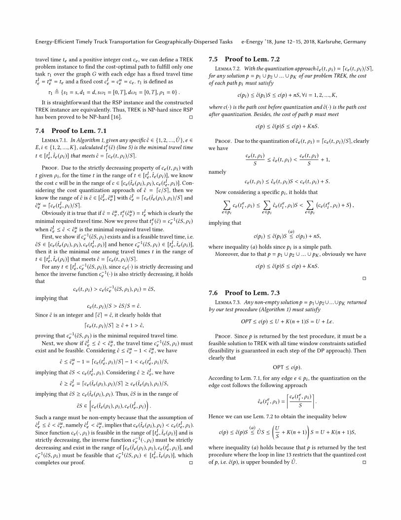
7 APPENDIX7.1 Summary of Key NotationsWe summarize key notations in Tab. 5.

7.2 Dynamic Programming For TREKIn this section we give algorithmic details of using DP to solve our

problem TREK which satisfies Bellman’s principle of optimality.

The DP approach has a pseudo-polynomial time complexity, and is

the foundation of our FPTAS introduced in Sec. 3.

In TREK, clearly the path travel time from si to di to fulfill τi inthe optimal solution must be upper bounded by β(dωi ) − α(sωi ). Ifwe denote pti as the path from si to di with the minimal cost and a

travel time upper bounded by t , the path in the optimal solution

Table 5: Summary of key notations.

Notations Definitions

G , (V ,E)The highway network G with connecting

points V and road segments E

fe (·) Fuel consumption rate function of e ∈ E

ce (·) Fuel consumption function of e ∈ E

De Distance of road segment e ∈ E

r le (resp. rue ) Minimum (resp. maximum) speed of e

t le (resp. tue ) Minimum (resp. maximum) travel time of e

cle (resp. cue )Minimum (resp. maximum) fuel

consumption of road segment e

te (ρ)The specific travel time t ∈ [t le , t

ue ] that

minimizes ce (·) given a truck load ρ

τi , i ∈ [1,K] The ith task

si (resp. di )Source node (resp. destination

node) of the ith task

sωi (resp. dωi )Source pickup window (resp. destination

delivery window) of the ith task

ρi Weight of cargos (load) of the ith task

α(sωi ) (resp.β(sωi ))

Earliest (resp. latest) pickup

time of the ith task

α(dωi ) (resp.β(dωi ))

Earliest (resp. latest) delivery

time of the ith task

σi , i ∈ [1,K + 1] Node si , or equivalently the node di−1

T outi (resp. T in

i )

Earliest leaving (resp. latest arrival) time

of node σi considering sωi and dωi−1

for the truck to fulfill τi must belong to the set Pi defined by

Pi ,{pti : ∀t ∈ (0, β(dωi ) − α(sωi )]

},

In order to solve TREK, we divide it to two sub-problems: (i) we

first obtain Pi for each τi , and (ii) we then figure out the solution

to TREK by selecting exactly one path pi from Pi for each task τiwith the combined solution p = p1 ∪ p2... ∪ pK meeting all time

window constraints and minimizing the total cost. We observe both

sub-problems meet the Bellman’s principle of optimality and thus

can be solved by DP.

7.2.1 Sub-Problem 1: Obtain Pi for Each τi . If we require eachedge travel time to be integral, for the task τi , let us define Ci (v,T )to be the minimal path cost of all paths from si to v with travel

time bounded above by T for the truck with load ρi . This enablesus to write the principle of optimality equation as

Ci (v,T ) = min

Ci (v,T − 1), min

{u,t }∈Mi (v,T )

{Ci (u,T − t) + c(u,v)(t , ρi )

} ,(12)

withMi (v,T ) defined as

Mi (v,T ) , {{u, t} : ∀u ∈ V s.t. ∃e = (u,v) ∈ E.∀t s.t. t ≤ T ,

t ∈[t le , te (ρi )

], t ∈ Z+},

and boundary conditions

Ci (si ,T ) = 0,∀T = 0, 1, ..., β(dωi ) − α(sωi ),

https://cumminsengines.com/uploads/docs/cummins_secrets_of_better_fuel_economy.pdf

https://cumminsengines.com/uploads/docs/cummins_secrets_of_better_fuel_economy.pdf

http://www.afdc.energy.gov/data/10312

https://developer.here.com/api-explorer/rest/traffic/flow-using-corridor

https://developer.here.com/api-explorer/rest/traffic/flow-using-corridor

http://www.kenworth.com/trucks/t800

http://cmap.m-plex.com/

http://cmap.m-plex.com/

https://freight.uber.com/

http://nationalmap.gov/epqs/

https://www.uship.com/


Ci (v, 0) = +∞,∀v ∈ V \{si }.

The Bellman’s equation (12) states that for a single task τi , theminimal cost from si to a certain node v with travel time upper

bounded by T is the smaller one comparing (i) the minimal cost

from si to v with travel time bounded above by T − 1, and (ii) the

minimal cost from si to a nodeu with travel time upper bounded by

T − t , plus the minimal cost to pass the edge (u,v) with travel time

no larger than t . Clearly, Ci (di , t) is the cost of the pathpti which can

be obtained recursively following the Bellman’s equation (12). Such

a DP approach has a pseudo-polynomial time complexity because

its size is polynomial with the β(dωi ), but exponential with the bit

length of the input, i.e. log (β(dωi )).Instead of integer travel time, if only cost is required to be inte-

gral, similar Bellman’s equation exits. We define Ti (v,C) to be the

minimal path travel time of all paths from si tov with cost bounded

above by C for the truck with load ρi . Then we have:

Ti (v,C) = min

Ti (v,C − 1), min

{u,c }∈Ni (v,C)

{Ti (u,C − c) + c−1

(u,v)(c, ρi )} ,(13)

with Ni (v,C) defined as

Ni (v,C) , {{u, c} : ∀u ∈ E s.t. ∃e = (u,v) ∈ E.∀c s.t. c ≤ C,

c ∈

[ce (te (ρi ), ρi ), ce (t

le , ρi )

], c ∈ Z+},

and boundary conditions

Ti (si ,C) = 0,∀C = 0, 1, ...,Cmax,

Ti (v, 0) = +∞,∀v ∈ V \{si },

where Cmax is an upper bound for the cost in the optimal solu-

tion from si to di to fulfill τi , e.g. it can be n · cmax : cmax =

maxe ∈E cue . For the Bellman’s equation (13), the cost of pti clearly

is min0≤C≤Cmax{C : Ti (di ,C) ≤ t}.

7.2.2 Sub-Problem 2: the Combined Solution. In sub-problem 1,

for each τi , we have achieved Pi through obtaining either all the

travel-time-bounded optimal cost Ci (di ,T ), or all the cost-boundedoptimal travel time Ti (di ,C). Our sub-problem 2 requires to pick

exactly one pi from each Pi such that the combined solution p =p1 ∪ p2... ∪ pK can optimize the total cost with all time window

constraints satisfied. We propose to use DP to solve sub-problem 2.

With integer travel time assumption, we define C(σi ,T ) as mini-

mal cost after the truck has fulfilled tasks from τ1 to τi−1 with all

associated time window satisfied, given that the truck is now at σiwhen the time is T . Then the principle of optimality equation is

C(σi ,T ) =

{min {C(σi ,T − 1),C∗(σi ,T )} , T ≤ T in

i ;

C(σi ,Tini ), otherwise,

(14)

where the definition of C∗(σi ,T ) is

C∗(σi ,T ) = min

t ∈Z+,t ≤T ,T−t ≥T out

i−1

{C(σi−1,T − t) + Ci−1(di−1, t)} ,

where Ci−1(di−1, t) is the same defined as in the equation (12). Note

that in the above definition constraintT − t ≥ T outi−1

guarantees that

the truck cannot leave σi−1 before the allowed earliest leaving time.

The boundary conditions are

C(σ1,T ) = 0,∀T = 0, 1, ...,T inK+1

C(σi , 0) = +∞,∀i = 2, 3, ...,K + 1.

Clearly C(σK+1,TinK+1

) gives optima to TREK. The feasibility is

guaranteed in each step of the DP where both earliest leaving time

and latest arrival time are satisfied in the equation (14). Similar

to sub-problem 1, the time complexity of the DP targeting sub-

problem 2 is pseudo-polynomial due to that it is exponential with

the bit length of the input time window constraint, i.e. log

(T inK+1

).

If we instead only require the edge cost to be integral, similar

Bellman’s equation also exists in our sub-problem 2. We define

T(σi ,C) as the earliest arrival time at node σi with cost bounded

above byC , in order to pick up the task τi after the truck has fulfilledthe tasks from τ1 to τi−1 within associated time windows. Then the

principle of optimality is

T(σi ,C) = min

{T(σi ,C − 1), min

c ∈Z+,c≤CT ∗(σi , c,C)

}, (15)

where T ∗(σi , c,C) is

T ∗(σi , c,C) =

{T , T ≤ T in

i ;

+∞, otherwise,

T = max

{T(σi−1,C − c),T out

i−1

}+ Ti−1(di−1, c).

In equation (15), T ∗(σi , c,C) is the earliest arrival time at σi witha cost bound C considering the case where the truck first arrives

at σi−1 with a cost upper bound C − c and then drives from σi−1

to σi fulfilling the task τi−1 with the associated path cost bounded

above by c . In the definition of T ∗(σi , c,C), earliest leaving time is

satisfied by comparing the T(σi−1,C − c) with the constraint T outi−1

,

and latest arrival time is also satisfied since we set T ∗(σi , c,C) tobe infinity if the truck arrives at σi later than the allowed latest

arrival time. The boundary conditions are

T(σ1,C) = 0,∀C = 0, 1, ...,KCmax,

T(σi , 0) = +∞,∀i = 2, 3, ...,K + 1,

where Cmax is the same defined as in the equation (13) and hence

KCmax is an upper bound for the optimal travel cost of TREK. Fol-lowing Bellman’s equation (15), the optimal solution of TREK with

the requirement of integer edge cost is defined clearly by

OPT = min

0≤C≤KCmax

{C : T(σK+1,C) ≤ T in

K+1

}.

Although proposed DP approach in this section requires either

integer travel time or integer cost, with proper rounding and scaling

technique, it can achieve solutions with performance guarantee

for general TREK instances without integer time/cost assumptions,

which is the key idea of our FPTAS designed in Sec. 3.

7.3 Proof to Thm. 2.1We prove our problem TREK is NP-hard in this section.

Proof. Following the definition of RSP described in [7], given

any RSP instance with input {G, s,d,T } where G is the graph, s(resp. d) is the source (resp. destination) node, T is the travel time

upper bound from s to d , each edge e ∈ E has a positive integer


travel time te and a positive integer cost ce , we can define a TREKproblem instance to find the cost-optimal path to fulfill only one

task τ1 over the graph G with each edge has a fixed travel time

t le = tue = te and a fixed cost cle = cue = ce . τ1 is defined as

τ1 , {s1 = s,d1 = d, sω1 = [0,T ],dω1 = [0,T ], ρ1 = 0} .

It is straightforward that the RSP instance and the constructed

TREK instance are equivalently. Thus, TREK is NP-hard since RSPhas been proved to be NP-hard [16]. �

7.4 Proof to Lem. 7.1Lemma 7.1. In Algorithm 1, given any specific c ∈ {1, 2, ..., U }, e ∈

E, i ∈ {1, 2, ...,K}, calculated tei (c) (line 5) is the minimal travel timet ∈ [t le , te (ρi )] that meets c = ⌈ce (t , ρi )/S⌉.

Proof. Due to the strictly decreasing property of ce (t , ρi ) with

t given ρi , for the time t in the range of t ∈ [t le , te (ρi )], we know

the cost c will be in the range of c ∈ [ce (te (ρi ), ρi ), ce (tle , ρi )]. Con-

sidering the cost quantization approach of c = ⌈c/S⌉, then we

know the range of c is c ∈ [cle , cue ] with c

le = ⌈ce (te (ρi ), ρi )/S⌉ and

cue = ⌈ce (tle , ρi )/S⌉.

Obviously it is true that if c = cue , tei (c

ue ) = t le which is clearly the

minimal required travel time. Nowwe prove that tei (c) = c−1

e (cS, ρi )

when cle ≤ c < cue is the minimal required travel time.

First, we show if c−1

e (cS, ρi ) exists and is a feasible travel time, i.e.

cS ∈ [ce (te (ρi ), ρi ), ce (tle , ρi )] and hence c−1

e (cS, ρi ) ∈ [t le , te (ρi )],then it is the minimal one among travel times t in the range of

t ∈ [t le , te (ρi )] that meets c = ⌈ce (t , ρi )/S⌉.

For any t ∈ [t le , c−1

e (cS, ρi )), since ce (·) is strictly decreasing and

hence the inverse function c−1

e (·) is also strictly decreasing, it holds

that

ce (t , ρi ) > ce (c−1

e (cS, ρi ), ρi ) = cS,

implying that

ce (t , ρi )/S > cS/S = c .

Since c is an integer and ⌈c⌉ = c , it clearly holds that

⌈ce (t , ρi )/S⌉ ≥ c + 1 > c,

proving that c−1

e (cS, ρi ) is the minimal required travel time.

Next, we show if cle ≤ c < cue , the travel time c−1

e (cS, ρi ) must

exist and be feasible. Considering c ≤ cue − 1 < cue , we have

c ≤ cue − 1 = ⌈ce (tle , ρi )/S⌉ − 1 < ce (t

le , ρi )/S,

implying that cS < ce (tle , ρi ). Considering c ≥ cle , we have

c ≥ cle = ⌈ce (te (ρi ), ρi )/S⌉ ≥ ce (te (ρi ), ρi )/S,

implying that cS ≥ ce (te (ρi ), ρi ). Thus, cS is in the range of

cS ∈

[ce (te (ρi ), ρi ), ce (t

le , ρi )

).

Such a range must be non-empty because that the assumption of

cle ≤ c < cue , namely cle < cue , implies that ce (te (ρi ), ρi ) < ce (tle , ρi ).

Since function ce (·, ρi ) is feasible in the range of [t le , te (ρi )] and is

strictly decreasing, the inverse function c−1

e (·, ρi ) must be strictly

decreasing and exist in the range of [ce (te (ρi ), ρi ), ce (tle , ρi )], and

c−1

e (cS, ρi ) must be feasible that c−1

e (cS, ρi ) ∈ [t le , te (ρi )], whichcompletes our proof. �

7.5 Proof to Lem. 7.2Lemma 7.2. With the quantization approach ce (t , ρi ) = ⌈ce (t , ρi )/S⌉,

for any solution p = p1 ∪ p2 ∪ ... ∪ pK of our problem TREK, the costof each path pi must satisfy

c(pi ) ≤ c(pi )S ≤ c(p) + nS,∀i = 1, 2, ...,K ,

where c(·) is the path cost before quantization and c(·) is the path costafter quantization. Besides, the cost of path p must meet

c(p) ≤ c(p)S ≤ c(p) + KnS .

Proof. Due to the quantization of ce (t , ρi ) = ⌈ce (t , ρi )/S⌉, clearlywe have

ce (t , ρi )

S≤ ce (t , ρi ) <

ce (t , ρi )

S+ 1,

namely

ce (t , ρi ) ≤ ce (t , ρi )S < ce (t , ρi ) + S .

Now considering a specific pi , it holds that∑e ∈pi

ce (tei , ρi ) ≤

∑e ∈pi

ce (tei , ρi )S <

∑e ∈pi

(ce (t

ei , ρi ) + S

),

implying that

c(pi ) ≤ c(pi )S(a)≤ c(pi ) + nS,

where inequality (a) holds since pi is a simple path.

Moreover, due to that p = p1 ∪ p2 ∪ ... ∪ pK , obviously we have

c(p) ≤ c(p)S ≤ c(p) + KnS .

�

7.6 Proof to Lem. 7.3Lemma 7.3. Any non-empty solutionp = p1∪p2∪ ...∪pK returned

by our test procedure (Algorithm 1) must satisfy

OPT ≤ c(p) ≤ U + K(n + 1)S = U + Lϵ .

Proof. Since p is returned by the test procedure, it must be a

feasible solution to TREKwith all time window constraints satisfied

(feasibility is guaranteed in each step of the DP approach). Then

clearly that

OPT ≤ c(p).

According to Lem. 7.1, for any edge e ∈ pi , the quantization on the

edge cost follows the following approach

ce (tei , ρi ) =

⌈ce (t

ei , ρi )

S

⌉.

Hence we can use Lem. 7.2 to obtain the inequality below

c(p) ≤ c(p)S(a)≤ U S ≤

(U

S+ K(n + 1)

)S = U + K(n + 1)S,

where inequality (a) holds because that p is returned by the test

procedure where the loop in line 13 restricts that the quantized cost

of p, i.e. c(p), is upper bounded by U . �


7.7 Proof to Lem. 7.4Lemma 7.4. If U ≥ OPT and our problem TREK is solvable, then

the test procedure (Algorithm 1) must return a non-empty solutionp = p1 ∪ p2 ∪ ... ∪ pK . Moreover, it holds for p that

c(p) ≤ OPT + Lϵ .

Proof. We denote the optimal solution to TREK by p∗ = p∗1∪

p∗2∪ ... ∪ p∗K with edge travel time tei (∗) for e ∈ p∗i . Define

tei , min

t ∈[t le ,t ei (∗)]t : ce (t , ρi ) = c

(tei (∗), ρi

)=

⌈c(tei (∗), ρi )

S

⌉,

which is the minimal travel time that shares the same quantized

cost compared to tei (∗), or equivalently the calculated tei (c) in line 5

of Algorithm 1 when c = ⌈c(tei (∗), ρi )/S⌉. Then we can define a

feasible solution p which has the same topology as p∗ but assigns atravel time of tei instead of tei (∗) to the edge e ∈ pi ,∀i = 1, 2, ...,K .The feasibility of p comes from that no edge travel time is increased

compared to the optimal solution p∗. And obviously it holds that

c(p) = c(p∗), c(pi ) = c(p∗i ),∀i = 1, 2, ...,K .

Considering the assumption ofU ≥ OPT = c(p∗), obviously thatU ≥ c(p∗i ),∀i = 1, 2, ...,K due to the non-negative property of edge

cost. Further according to Lem. 7.2, for any i ∈ 1, 2, ...,K , we have

c(pi ) = c(p∗i ) ≤

c(p∗i )

S+ n ≤

⌊c(p∗i )

S

⌋+ n + 1 ≤ U .

Similarly we can prove that c(p) = c(p∗) ≤ U . Therefore, pi must

be examined in the loop (line 8) of Algorithm 1, and hence p must

be examined in the loop (line 13) of Algorithm 1. Due to that pis a feasible solution to TREK, the test procedure must return a

non-empty solution p which may be different from p.Since p is the optimal solution to the test procedure, it must hold

that c(p) ≤ c(p). According to Lem. 7.2, we have

c(p) ≤ c(p)S ≤ c(p)S = c(p∗)S ≤ c(p∗) + KnS ≤ OPT + Lϵ .

�

7.8 Proof to Lem. 7.5Lemma 7.5. Algorithm 1 has a time complexity of O(Knm(Kn +

UKnLϵ )2), assuming it takes a constant time to calculate te (ρi ), ce (t , ρi )

and c−1

e (c, ρi ) given an edge e ∈ E and a truck load ρi .

Proof. There are three loops in Algorithm 1. First loop of line 3

has a time complexity of O(KmU ). Second loop of line 8 has a time

complexity ofO(KnmU 2). Third loop of line 13 has a time complex-

ity of O(KU 2). Overall, our algorithm 1 has a time complexity of

O(KnmU 2) = O(Knm(Kn + UKnLϵ )2). �

7.9 Proof to Lem. 7.6Lemma 7.6. If Test(G, ®σ ,B,B, 1) returns NULL, OPT ≥ B. Other-

wise, if Test(G, ®σ ,B,B, 1) returns a non-empty solution, OPT ≤ 2B.

Proof. According to Lem. 7.4, if OPT < B, Test(G, ®σ ,B,B, 1)must return a non-empty solution. Thus if the test returns NULL,it holds that OPT ≥ B.

According to Lem. 7.3, for the returned non-empty solution p of

Test(G, ®σ ,B,B, 1), we have

OPT ≤ U + Lϵ = 2B.

�

7.10 Proof to Thm. 3.1Weprove our FPTAS in Algorithm 2 provides a (1+ϵ)-approximation

ratio in this section.

Proof. According to Lem. 7.6, in the binary search scheme of

line 3, our Algorithm 2 always maintain a valid lower bound BLand a valid upper bound 2BU for OPT till the gap BU /BL ≤ 2.

Therefore, in line 9, since 2BU is a valid upper bound of OPT,according to Lem. 7.4, Test(G, ®σ ,BL , 2BU , ϵ) must return a non-

empty solution pfptas that satisfies

c(pfptas) ≤ OPT + BLϵ ≤ (1 + ϵ)OPT.

�

7.11 Proof to Thm. 4.1In this section, we prove the equivalence of two formulations of

problem TREK: formulation (2) and formulation (4).

Proof. Since both formulations share the same objective func-

tion, we only need to prove that a solution ®xi , ®ti , i = 1, 2, ...,K is

feasible in terms of formulation (2) if and only if it is feasible in

terms of formulation (4),

If part. Suppose ®xi , ®ti , i = 1, 2, ...,K satisfies the constraint (4b),

we prove it must satisfy the constraint (2b).

For such a solution ®xi , ®ti , i = 1, 2, ...,K , given a specific i ∈

1, 2, ....K , if ai−1 ≤ T outi , then we have

max

{ai−1,T

outi

}+

∑e ∈E

xei tei = T

outi +

∑e ∈E

xei tei .

Based on the constraint (4b) when r = k = i , clearly it holds that

max

{ai−1,T

outi

}+

∑e ∈E

xei tei ≤ T out

i +T ini+1

−T outi = T in

i+1,

which is the constraint (2b).

If ai−1 > Touti , without loss of generality, we assume that aj >

T outj+1

for j = l , l + 1, ..., i − 1 where l ≥ 1 and al−1≤ T out

l . Then it

holds that

max{ai−1,Touti } +

∑e ∈E

xei tei = ai−1 +

∑e ∈E

xei tei

= ai−2 +∑e ∈E

xei−1tei−1+

∑e ∈E

xei tei

= ...

= al +i∑

j=l+1

∑e ∈E

xej tej

= T outl +

i∑j=l

∑e ∈E

xej tej .


Based on the constraint (4b) when r = i,k = l , namely the con-

straint of

∑ij=l

∑e ∈E x

ej tej ≤ T in

i+1−T out

l , obviously it holds that

max

{ai−1,T

outi

}+

∑e ∈E

xei tei ≤ T out

l +T ini+1

−T outl = T in

i+1,

which is the constraint (2b).

Only if part. Assume ®xi , ®ti , i = 1, 2, ...,K satisfies the con-

straint (2b), we prove it must satisfy the constraint (4b).

Due to our assumption that ai = max{ai−1,Touti } +

∑e ∈E x

ei t

ei

and ai ≤ T ini+1

, considering the two inequality max{ai−1,Touti } ≥

ai−1 and max{ai−1,Touti } ≥ T out

i , for any r = 1, 2, ...,K and any

k = 1, 2, ..., r , we have∑e ∈E

xer ter ≤ T in

r+1− max

{ar−1,T

outr

},

≤ T inr+1

− ar−1

= T inr+1

− max

{ar−2,T

outr−1

}−

∑e ∈E

xer−1ter−1

≤ T inr+1

−∑e ∈E

xer−1ter−1

− ar−2

= T inr+1

−

r−1∑j=r−2

∑e ∈E

xej tej − max

{ar−3,T

outr−2

}≤ ...

= T inr+1

−

r−1∑j=k

∑e ∈E

xej tej − max

{ak−1,T outk

}≤ T in

r+1−

r−1∑j=k

∑e ∈E

xej tej −T out

k ,

namely it holds that

r∑j=k

xej tej ≤ T in

r+1−T out

k ,

which is the constraint (4b). �

7.12 Proof to Thm. 4.2We prove our Thm. 4.2 in this section, namely

D(®λ) = −

K∑r=1

r∑k=1

λrk (Tinr+1

−T outk ) +

K∑i=1

∑e ∈p(µi )

wei (µi ).

Proof.

D(®λ) = min

®x, ®tL(®x , ®t , ®λ)

= −

K∑r=1

r∑k=1

λrk (Tinr+1

−T outk )

+min

®x, ®t

K∑i=1

∑e ∈E

xei ·[ce (t

ei , ρi ) + µi t

ei]

(a)= −

K∑r=1

r∑k=1

λrk (Tinr+1

−T outk )

+

K∑i=1

min

®ximin

®ti

∑e ∈E

xei ·[ce (t

ei , ρi ) + µi t

ei]

(b)= −

K∑r=1

r∑k=1

λrk (Tinr+1

−T outk )

+

K∑i=1

min

®xi

∑e ∈E

xei · min

t le ≤t ei ≤te (ρi )

[ce (t

ei , ρi ) + µi t

ei]

(c)= −

K∑r=1

r∑k=1

λrk (Tinr+1

−T outk )

+

K∑i=1

min

®xi

∑e ∈E

xei ·[ce (t

ei (µi ), ρi ) + µi t

ei (µi )

](d )= −

K∑r=1

r∑k=1

λrk (Tinr+1

−T outk ) +

K∑i=1

min

®xi

∑e ∈E

xei ·wei (µi )

(e)= −

K∑r=1

r∑k=1

λrk (Tinr+1

−T outk ) +

K∑i=1

∑e ∈p(µi )

wei (µi ),

where equality (a) holds because no coupled constraints exist for

different tasks and further no coupled constraints exist between

®xi and ®ti given any i = 1, 2, ...,K . Equality (b) is true because nocoupled constraints exist for the travel time on different edges given

any i = 1, 2, ...,K . Equality (c) holds due to our definition of tei (µi ).Similarly, equality (d) is true due to our definition ofwe

i (µi ), andequality (e) holds due to the definition of p(µi ). �

7.13 Proof to Thm. 4.4Proof. First we prove the solution {p(µi ), i = 1, 2, ...,K} that

meets condition (10) must be a feasible solution to TREK.Obviously for each task τi , i = 1, 2, ...,K , such a solution de-

fines a path from σi to σi+1 to fulfill τi . Hence in order to prove its

feasibility, we only need to prove it satisfies all the time window

constraint (4b). For any r = 1, 2, ...,K and k = 1, 2, ..., r , if the corre-sponding λrk is strictly positive, clearly based on the condition (10)

we have

T outk −T in

r+1+

r∑j=k

δ (µ j ) = 0,

implying that the solution {p(µi ), i = 1, 2, ...,K} meets the con-

straint (4b). For any r = 1, 2, ...,K and k = 1, 2, ..., r , if the corre-sponding λrk = 0, based on the condition (10) we have

max

T outk −T in

r+1+

r∑j=k

δ (µ j ), 0

= 0,

namely it holds that

T outk −T in

r+1+

r∑j=k

δ (µ j ) ≤ 0,

also proving that the solution {p(µi ), i = 1, 2, ...,K} meets the

constraint (4b). Overall, the solution {p(µi ), i = 1, 2, ...,K} must be

feasible, and hence provides an upper bound for the optimal cost


OPT of problem TREK, i.e.

P(®λ) =K∑i=1

∑e ∈p(µi )

ce (tei (µi ), ρi ) ≥ OPT. (16)

Next we look at the dual function value of the solution {p(µi ), i =1, 2, ...,K}.

D(®λ) = −

K∑r=1

r∑k=1

λrk (Tinr+1

−T outk )

+

K∑i=1

∑e ∈p(µi )

[ce (t

ei (µi ), ρi ) + µi t

ei (µi )

]= −

K∑r=1

r∑k=1

λrk (Tinr+1

−T outk )

+

K∑i=1

µiδ (µi ) +K∑i=1

∑e ∈p(µi )

ce (tei (µi ), ρi )

=

K∑r=1

r∑k=1

λrk ·©«T out

k −T inr+1+

r∑j=k

δ (µ j )ª®¬

+

K∑i=1

∑e ∈p(µi )

ce(tei (µi ), ρi

).

Since the condition (10) implies that

λrk ·©«T out

k −T inr+1+

r∑j=k

δ (µ j )ª®¬ = 0,

∀r = 1, 2, ...,K ,∀k = 1, 2, ..., r ,

the dual function is equal to

D(®λ) =K∑i=1

∑e ∈p(µi )

ce (tei (µi ), ρi ).

According to the weak duality, any dual function value is a lower

bound of the optimal cost OPT, namely it holds that

D(®λ) =K∑i=1

∑e ∈p(µi )

ce (tei (µi ), ρi ) ≤ OPT. (17)

Comparing the inequality (16) and the inequality (17), obviously

that the solution {p(µi ), i = 1, 2, ...,K} must be optimal to problem

TREK. �

7.14 Proof to Thm. 4.5We prove our Thm. 4.5 in this section, namely prove the perfor-

mance bound of SPEED in Algorithm 3.

Proof. If TREK is solvable, the solution where each task is ful-

filled by the fastest path must be feasible, which must be examined

by SPEED due to that initially we set all dual variables to be a large

enough λmax. Therefore, SPEED must return a feasible solution.

Result for case 1 holds directly due to Thm. 4.4.

For p returned in case 2, let us denote the dual variables defining

p as¯λrk ,∀r = 1, 2, ...,K ,∀k = 1, 2, ..., r , and denote max∀r,k | Ûλrk | as

Ûλ, namely | Ûλrk | ≤Ûλ,∀r = 1, 2, ...,K ,∀k = 1, 2, ..., r .

Because p is feasible, we have

P(®λ) =K∑i=1

∑e ∈p(µi )

ce(tei (µi ), ρi

)≥ OPT. (18)

Next we look at the dual function value of p.

D( ®λ) = −

K∑r=1

r∑k=1

¯λrk (Tinr+1

−T outk )

+

K∑i=1

µiδ (µi ) +K∑i=1

∑e ∈p(µi )

ce(tei (µi ), ρi

)=

K∑r=1

r∑k=1

¯λrk ·©«T out

k −T inr+1+

r∑j=k

δ (µ j )ª®¬

+

K∑i=1

∑e ∈p(µi )

ce(tei (µi ), ρi

).

Since p is feasible meeting all constraints in our formulation (4):

r∑j=k

δ (µ j ) ≤ T inr+1

−T outk ,∀r = 1, 2, ...,K ,∀k = 1, 2, ..., r ,

it holds that T outk −T in

r+1+

r∑j=k

δ (µ j )

+

¯λrk

≤ 0.

Further due to ϕ( ¯λrk ) > 0, it holds thatÛλrk ≤ 0, implying that

− Ûλ ≤ Ûλrk ≤ 0, and we haveT outk −T in

r+1+

r∑j=k

δ (µ j )

+

¯λrk

≥ − Ûλ/ϕ( ¯λrk ).

Considering definition of [T outk −T in

r+1+

∑rj=k δ (µ j )]

+¯λrk, we have

¯λrk©«T out

k −T inr+1+

r∑j=k

δ (µ j )ª®¬ = ¯λrk

T outk −T in

r+1+

r∑j=k

δ (µ j )

+

¯λrk

≥ − Ûλ · ¯λrk/ϕ(¯λrk ).

According to the weak duality, it holds that

D( ®λ) ≤ OPT. (19)

Comparing the inequality (18) and the inequality (19), we have:

P(®λ) − OPT ≤ P(®λ) − D( ®λ)

= −

K∑r=1

r∑k=1

¯λrk ·©«T out

k −T inr+1+

r∑j=k

δ (µ j )ª®¬

≤ K2 · Ûλ · max∀r,k{

¯λrk/ϕ(¯λrk )

}= K2 · max∀r,k

�� Ûλrk �� · max∀r,k{

¯λrk/ϕ(¯λrk )

}.

�

energy-efficient timely truck transportation for

Documents