University of Nebraska - Lincoln University of Nebraska - Lincoln

DigitalCommons@University of Nebraska - Lincoln DigitalCommons@University of Nebraska - Lincoln

Computer Science and Engineering: Theses, Dissertations, and Student Research

Computer Science and Engineering, Department of

4-2013

Energy-efficient Failure Recovery in Hadoop Cluster Energy-efficient Failure Recovery in Hadoop Cluster

Weiyue Xu University of Nebraska – Lincoln, weiyue@cse.unl.edu

Follow this and additional works at: https://digitalcommons.unl.edu/computerscidiss

Part of the Computer Engineering Commons, and the Other Computer Sciences Commons

Xu, Weiyue, "Energy-efficient Failure Recovery in Hadoop Cluster" (2013). Computer Science and Engineering: Theses, Dissertations, and Student Research. 56. https://digitalcommons.unl.edu/computerscidiss/56

This Article is brought to you for free and open access by the Computer Science and Engineering, Department of at DigitalCommons@University of Nebraska - Lincoln. It has been accepted for inclusion in Computer Science and Engineering: Theses, Dissertations, and Student Research by an authorized administrator of DigitalCommons@University of Nebraska - Lincoln.

ENERGY-EFFICIENT FAILURE RECOVERY IN HADOOP CLUSTER

by

Weiyue Xu

A THESIS

Presented to the Faculty of

The Graduate College at the University of Nebraska

In Partial Fulfilment of Requirements

For the Degree of Master of Science

Major: Computer Science

Under the Supervision of Professors Ying Lu

Lincoln, Nebraska

May, 2013

ENERGY-EFFICIENT FAILURE RECOVERY IN HADOOP CLUSTER

Weiyue Xu, M. S.

University of Nebraska, 2013

Advisors: Ying Lu

Based on U.S. Environmental Protection Agency’s estimation, only in U.S., billions of

dollars are spent on the electricity cost of data centers each year, and the cost is continually

increasing very quickly. Energy efficiency is now used as an important metric for evaluating

a computing system. However, saving energy is a big challenge due to many constraints.

For example, in one of the most popular distributed processing frameworks, Hadoop, three

replicas of each data block are randomly distributed in order to improve performance and

fault tolerance, but such a mechanism limits the largest number of machine that can be

turned off to save energy without affecting the data availability. To overcome this limitation,

previous research introduces a new mechanism called covering subset which maintains a

set of active nodes to ensure the immediate availability of data, even when all nodes not in

the covering subset are turned off. This covering subset based mechanism works smoothly

if no failure happens. However, a node in the covering subset may fail.

In this thesis, we study the energy-efficient failure recovery in Hadoop clusters where

nodes are grouped into covering and non-covering subsets. Rather than only using the repli-

cation as adopted by a Hadoop system by default, we study both replication and erasure

coding as possible redundancy mechanisms. We first present a replication based greedy

failure recovery algorithm and then introduce an erasure coding based greedy failure re-

covery algorithm. Moreover, we also develop a recovery aware data placement strategy to

further improve the energy efficiency in failure recovery.

To evaluate the algorithms, we simulate node failure recovery in the clusters of differ-

ent sizes, construct the energy model and analyze the energy consumed during the failure

recovery process. The simulation results show that the erasure coding based failure recov-

ery algorithm often outperforms the replication based approach. On average, the former

requires 60% of the energy as that of the later and the energy saving increases with the

cluster size. In addition, with our recovery aware data placement strategy, the energy con-

sumption for both approaches could be further reduced.

iv

ACKNOWLEDGMENTS

I would like to express my sincere gratitude to my adviser Dr. Ying Lu for her patience,

guidance, support, and enthusiastic help. She is a wonderful adviser and mentor who al-

ways encourages me and guides me to find suitable solutions for problems I have faced not

only in academia but also in life. This thesis cannot be completed without her help.

I also want to appreciate my minor adviser, Dr. Allan McCutcheon, whose earnest and

enthusiastic attitude on work and life always create positive energy for me, and I appre-

ciate Dr. David Swanson who serves as my master’s thesis committee and takes time on

reviewing my thesis.

There are many people at UNL that deserve my wholehearted thanks as well, they give

me suggestions and help me adapt to life in Lincoln. Especially, I am grateful to Chen He,

who helped me in collecting the power consumption data in our testbed cluster.

At last, but certainly not the least, I must thank my parents for their love, inspiration

and support throughout my life. This thesis is dedicated to them.

v

Contents

Contents v

List of Figures vii

List of Tables ix

1 Introduction 1

2 Background and Related Work 5

2.1 Hadoop . . . . . . . . . . . . . . . . . . . . . . . . . . . . . . . . . . . . 5

2.1.1 Hadoop Distributed File System . . . . . . . . . . . . . . . . . . . 6

2.1.2 Hadoop MapReduce . . . . . . . . . . . . . . . . . . . . . . . . . 8

2.2 Data Redundancy Technologies . . . . . . . . . . . . . . . . . . . . . . . . 10

2.2.1 Erasure Coding . . . . . . . . . . . . . . . . . . . . . . . . . . . . 10

2.2.2 Replication vs. Erasure Coding . . . . . . . . . . . . . . . . . . . . 11

2.3 Related Work . . . . . . . . . . . . . . . . . . . . . . . . . . . . . . . . . 11

3 Problem Setting 14

3.1 System Model . . . . . . . . . . . . . . . . . . . . . . . . . . . . . . . . . 14

3.2 Node Failure and Recovery . . . . . . . . . . . . . . . . . . . . . . . . . . 15

vi

4 Failure Recovery Algorithms 17

4.1 Failure Recovery with Replication Based Extended Set . . . . . . . . . . . 18

4.2 Failure Recovery with Erasure-Coding-Based Extended Set . . . . . . . . . 22

4.3 Recovery Aware Data Placement Strategy . . . . . . . . . . . . . . . . . . 27

5 Energy Model 34

5.1 Energy spent in ES . . . . . . . . . . . . . . . . . . . . . . . . . . . . . . 35

5.2 Energy spent in FS . . . . . . . . . . . . . . . . . . . . . . . . . . . . . . 37

5.3 Energy spent in WS . . . . . . . . . . . . . . . . . . . . . . . . . . . . . . 41

5.4 Energy Consumption of the Two Approaches . . . . . . . . . . . . . . . . 41

6 Simulation 43

6.1 Energy consumption . . . . . . . . . . . . . . . . . . . . . . . . . . . . . 43

6.2 Simulation Results . . . . . . . . . . . . . . . . . . . . . . . . . . . . . . 45

7 Conclusion 58

8 Future Work 59

Bibliography 60

vii

List of Figures

2.1 Hadoop Base Platform [8] . . . . . . . . . . . . . . . . . . . . . . . . . . . . 6

2.2 HDFS Architecture [27] . . . . . . . . . . . . . . . . . . . . . . . . . . . . . . 7

2.3 Data placement in HDFS . . . . . . . . . . . . . . . . . . . . . . . . . . . . . 9

2.4 Erasure coding with d=3 and e=2 . . . . . . . . . . . . . . . . . . . . . . . . . 11

3.1 System Model . . . . . . . . . . . . . . . . . . . . . . . . . . . . . . . . . . . 15

5.1 Decoding and data transfer in a FS node . . . . . . . . . . . . . . . . . . . . . 40

6.1 Comparison on energy consumption of replication-based system vs erasure-

coding-based system (same fault tolerance level) . . . . . . . . . . . . . . . . . 47

6.2 Comparison on energy consumption of data placed replication-based systems

vs data placed erasure-coding-based systems (same fault tolerance level) . . . . 49

6.3 Comparison on energy consumption of replication-based systems with/without

recovery aware data placement enabled (same fault tolerance level) . . . . . . . 49

6.4 Comparison on energy consumption of erasure-coding-based systems with-

/without recovery aware data placement enabled (same fault tolerance level) . . 50

6.5 Comparison on energy consumption of replication-based system vs erasure-

coding-based system (same storage space) . . . . . . . . . . . . . . . . . . . . 51

viii

6.6 Comparison on energy consumption of data placed replication-based systems

vs data placed erasure-coding-based systems (same storage space) . . . . . . . 52

6.7 Comparison on energy consumption of data placed replication-based systems

vs data placed erasure-coding-based systems (same storage space) . . . . . . . 53

ix

List of Tables

6.1 Time spent by Jerasure’s erasure coding (e = 2) . . . . . . . . . . . . . . . . . 46

6.4 Time spent by Jerasure’s erasure coding(e = 2 ∗ d) . . . . . . . . . . . . . . . 50

6.2 Simulation results from recovering a node failure in clusters of different sizes(same

fault tolerance level) . . . . . . . . . . . . . . . . . . . . . . . . . . . . . . . . 54

6.3 Simulation results from recovering a node failure in clusters of different sizes

with recovery aware data placement strategy enabled (same fault tolerance level) 55

6.5 Simulation results from recovering a node failure in clusters of different sizes

(same storage space) . . . . . . . . . . . . . . . . . . . . . . . . . . . . . . . 56

6.6 Simulation results from recovering a node failure in clusters of different sizes

with recovery aware data placement strategy enabled (same storage space) . . . 57

1

Chapter 1

Introduction

Enormous data centers are built to support various types of data processing services like

email services and searching engine services. Data centers are becoming critical in modern

life. According to data center research organization Uptime Institute’s survey in May 2011,

36 percent of the large companies surveyed were expecting to exhaust IT capacity within

18 months. That means, they must enlarge their existing data centers or build more data

centers. To maintain a data center, a large amount of energy need to be consumed for both

computing and cooling [4]. It is reported that in 2010 2% of electricity is used by data

centers in US and 1.3% around the world [19]. As data centers continue to grow in size

and number, some researchers estimated that by 2012 the cost of electricity for data centers

could exceed the cost of the original capital investment [25]. As a result, how to achieve

energy efficiency is a major issue for data centers [2].

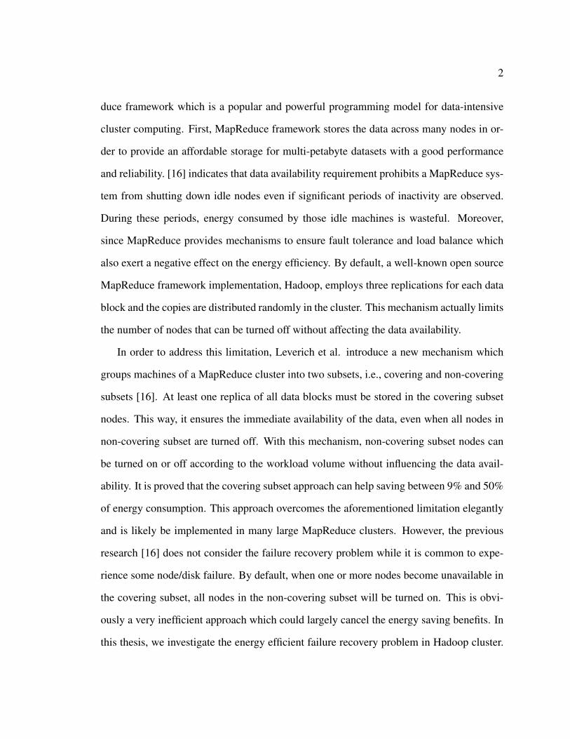
One typical and effective way for saving computing energy is to shut down idle ma-

chines. According to [6] and [20], there is a large portion of idle machines in data centers

consuming up to 60% of the total energy. In order to inactivate as many machines as possi-

ble to save energy, researchers attempt to dynamically match the number of activate nodes

with the current workload [6]. However, it is nontrivial to apply this approach to MapRe-

2

duce framework which is a popular and powerful programming model for data-intensive

cluster computing. First, MapReduce framework stores the data across many nodes in or-

der to provide an affordable storage for multi-petabyte datasets with a good performance

and reliability. [16] indicates that data availability requirement prohibits a MapReduce sys-

tem from shutting down idle nodes even if significant periods of inactivity are observed.

During these periods, energy consumed by those idle machines is wasteful. Moreover,

since MapReduce provides mechanisms to ensure fault tolerance and load balance which

also exert a negative effect on the energy efficiency. By default, a well-known open source

MapReduce framework implementation, Hadoop, employs three replications for each data

block and the copies are distributed randomly in the cluster. This mechanism actually limits

the number of nodes that can be turned off without affecting the data availability.

In order to address this limitation, Leverich et al. introduce a new mechanism which

groups machines of a MapReduce cluster into two subsets, i.e., covering and non-covering

subsets [16]. At least one replica of all data blocks must be stored in the covering subset

nodes. This way, it ensures the immediate availability of the data, even when all nodes in

non-covering subset are turned off. With this mechanism, non-covering subset nodes can

be turned on or off according to the workload volume without influencing the data avail-

ability. It is proved that the covering subset approach can help saving between 9% and 50%

of energy consumption. This approach overcomes the aforementioned limitation elegantly

and is likely be implemented in many large MapReduce clusters. However, the previous

research [16] does not consider the failure recovery problem while it is common to expe-

rience some node/disk failure. By default, when one or more nodes become unavailable in

the covering subset, all nodes in the non-covering subset will be turned on. This is obvi-

ously a very inefficient approach which could largely cancel the energy saving benefits. In

this thesis, we investigate the energy efficient failure recovery problem in Hadoop cluster.

3

Specifically, we study how to restore data with the lowest electricity cost when a node fails

in the covering subset.

In Hadoop, as well as most other well-known MapReduce implementations, replication

is the default redundancy mechanism used to achieve fault tolerance. Although straight-

forward, replication leads to high storage overhead. There is another common redundancy

technology, erasure coding (i.e., parity schema), which uses an order of magnitude less

storage than replication under the same fault tolerance level. However, it demands some

extra effort on encoding and decoding the data. Basically, erasure coding divides an object

into d fragments, which will be recoded into d + e fragments, where dd+e

< 1 represents

the rate of encoding. Erasure coding provides flexibility in failure recovery because any d

out of the d+ e fragments can be used for reconstructing the original d fragments.

In this thesis, we research on the problem of energy efficient failure recovery in Hadoop

cluster where only one data replica is kept online. Similar to the covering subset mechanism

in paper [16], we divide the Hadoop cluster into three sets, Fundamental Set (FS), Extended

Set(ES), and Waiting Set(WS). FS contains a group of active machines that store one replica

of all data blocks; WS holds several offline machines which could be used as backup if

some node fails in FS. ES maintains some inactivated nodes with redundant information

of the original data. Two different data redundancy technologies, replication and erasure

coding, are considered in our work. We develop greedy failure recovery algorithms based

on these two technologies. And according to analysis of the greedy algorithms, we propose

a recovery aware data placement policy which can further improve the efficiency of failure

recovery. To evaluate the energy efficiency of our algorithms, we build energy model and

simulate node failure in clusters of different sizes.

The rest of this thesis is organized as follows: in Chapter 2, background information,

including Hadoop Distributed File System (HDFS), Hadoop MapReduce and erasure cod-

ing are introduced and several related work are presented. Then, problem setting is given in

4

Chapter 3, after which, Chapter 4 characterizes two greedy algorithms: default replication

based failure recovery algorithm and erasure coding based failure recovery algorithm. Our

recovery aware data placement strategy is also described. Chapter 5 models the energy

consumption of failure recovery for the two systems of different redundancy technologies.

In Chapter 6, we use simulations to evaluate the two systems with and without recovery

aware data placement strategy enabled. Finally, Chapter 7 and Chapter 8 summarize our

work and propose the future work.

5

Chapter 2

Background and Related Work

One of the distinguished features of distributed system is the notion of partial failure [24].

A robust distributed system must be able to handle failure recovery automatically. In this

Chapter, we start with introducing Hadoop Distributed File System (HDFS) and Hadoop

MapReduce. Then, we describe and compare two commonly used data redundancy tech-

nologies: replication and erasure coding. Finally, we present some related research work.

2.1 Hadoop

Hadoop is a famous open-source framework that supports distributed processing of large-

scale data sets across a cluster of computers [12]. Many large companies like Facebook,

Yahoo!, and Amazon [10] are using Hadoop for processing big-data. Hadoop gains popu-

larity because of its outstanding scalability and high fault tolerance. Specifically, compar-

ing with traditional data center, Hadoop clusters have several advantages on data-intensive

computing: 1) it implements MapReduce framework to simplify the parallelism of users’

applications; 2) it uses commodity machines rather than high-budget servers to enhance

scalability and flexibility; 3) it tolerates faults at different levels, including disks, nodes,

6

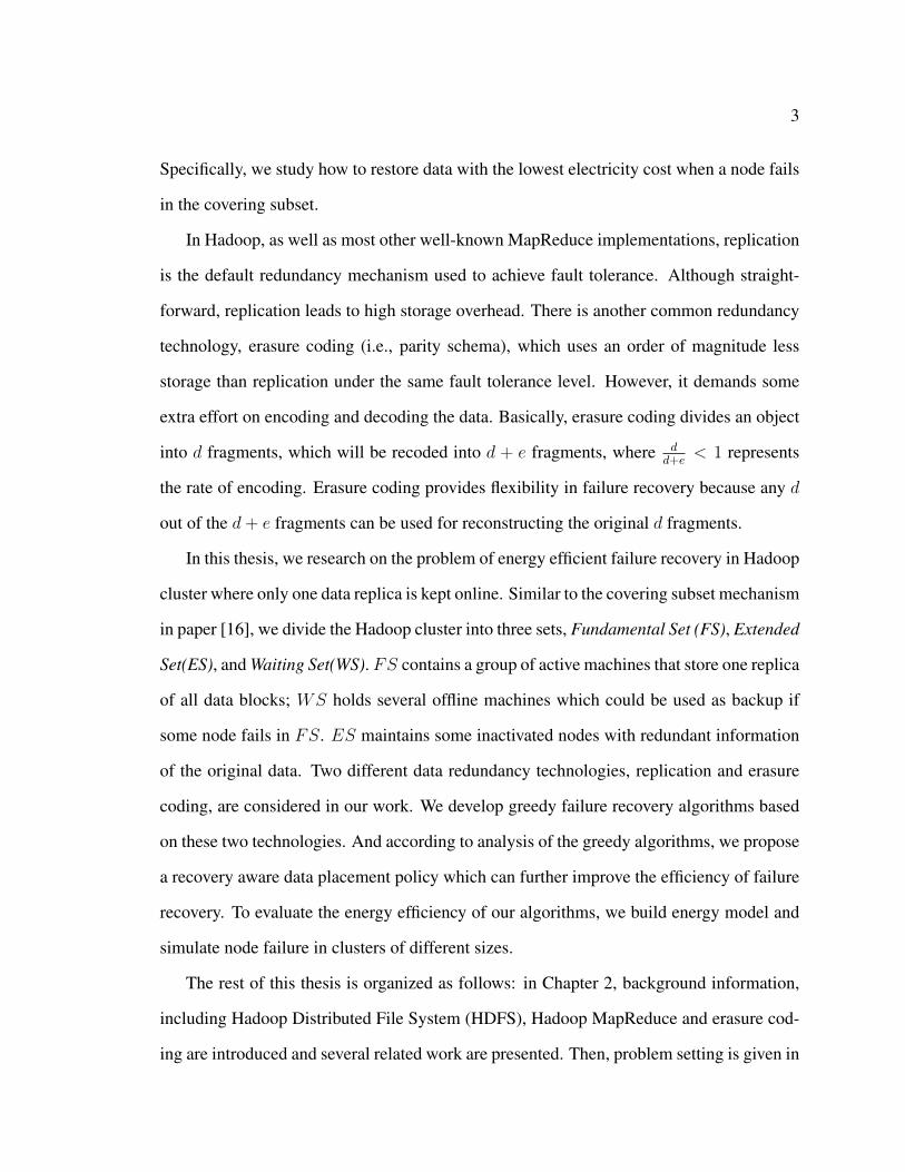
Figure 2.1: Hadoop Base Platform [8]

switches, networks, to improve the reliability. In this Chapter, we briefly describe the two

subsystems in Hadoop base platform, i.e., Hadoop Distributed File System (HDFS) and

Hadoop MapReduce [27]. Figure 2.1 depicts the collaboration between these two compo-

nents.

2.1.1 Hadoop Distributed File System

Our work focuses on the data availability in Hadoop. It is thus necessary to first understand

Hadoop distributed filesystem, HDFS. In this Chapter, we briefly introduce the architecture

and then describe the fault tolerance and data placement policy in HDFS.

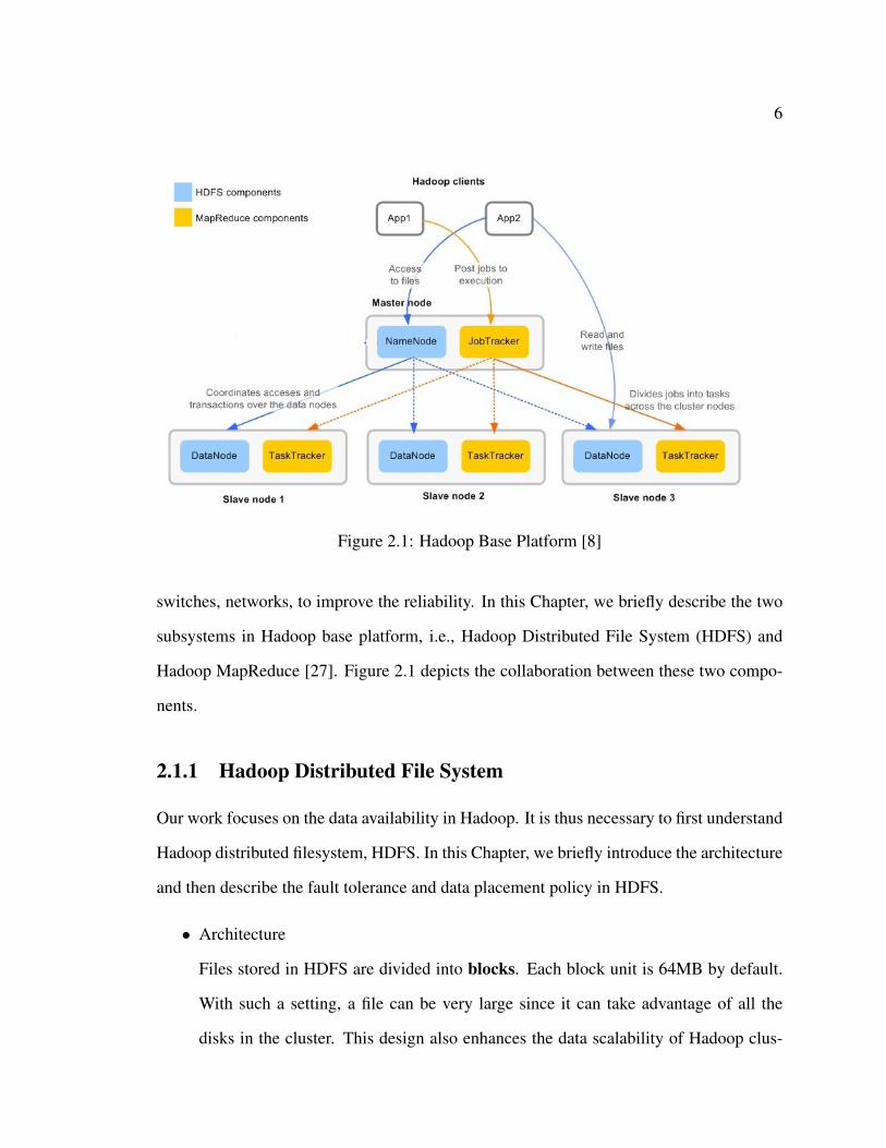
• Architecture

Files stored in HDFS are divided into blocks. Each block unit is 64MB by default.

With such a setting, a file can be very large since it can take advantage of all the

disks in the cluster. This design also enhances the data scalability of Hadoop clus-

7

Figure 2.2: HDFS Architecture [27]

ters. As illustrated in Figure 2.2, Hadoop cluster follows master-slave architecture.

In particular, there is a master node named Namenode with a number of slave nodes,

called Datanodes. In the cluster, Namenode maintains the file system namespace

and the metadata for all the files while the Datanodes store the blocks. Periodically,

every Datanode sends a heartbeat and a report of block list periodically to the Na-

menode such that Namenode can construct and update the “blocksMap” (a mapping

table which maps data blocks to Datanodes). Because Namenode has the data place-

ment information of all Datanodes, it coordinates access operations between clients

and Datanodes [8]. Finally, Datanodes are responsible for serving read and write

requests.

8

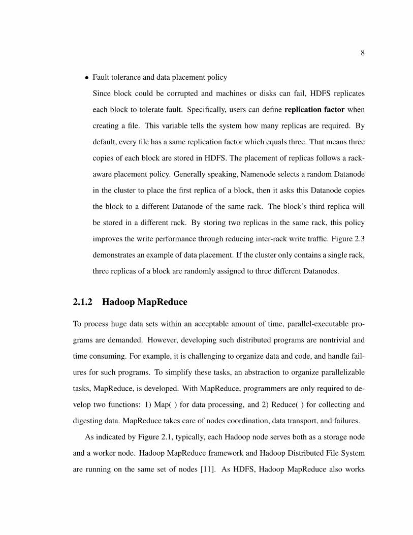
• Fault tolerance and data placement policy

Since block could be corrupted and machines or disks can fail, HDFS replicates

each block to tolerate fault. Specifically, users can define replication factor when

creating a file. This variable tells the system how many replicas are required. By

default, every file has a same replication factor which equals three. That means three

copies of each block are stored in HDFS. The placement of replicas follows a rack-

aware placement policy. Generally speaking, Namenode selects a random Datanode

in the cluster to place the first replica of a block, then it asks this Datanode copies

the block to a different Datanode of the same rack. The block’s third replica will

be stored in a different rack. By storing two replicas in the same rack, this policy

improves the write performance through reducing inter-rack write traffic. Figure 2.3

demonstrates an example of data placement. If the cluster only contains a single rack,

three replicas of a block are randomly assigned to three different Datanodes.

2.1.2 Hadoop MapReduce

To process huge data sets within an acceptable amount of time, parallel-executable pro-

grams are demanded. However, developing such distributed programs are nontrivial and

time consuming. For example, it is challenging to organize data and code, and handle fail-

ures for such programs. To simplify these tasks, an abstraction to organize parallelizable

tasks, MapReduce, is developed. With MapReduce, programmers are only required to de-

velop two functions: 1) Map( ) for data processing, and 2) Reduce( ) for collecting and

digesting data. MapReduce takes care of nodes coordination, data transport, and failures.

As indicated by Figure 2.1, typically, each Hadoop node serves both as a storage node

and a worker node. Hadoop MapReduce framework and Hadoop Distributed File System

are running on the same set of nodes [11]. As HDFS, Hadoop MapReduce also works

9

Figure 2.3: Data placement in HDFS

in master-slave mode. Specifically, there is a master node called JobTracker and many

slave nodes called TaskTrackers. Jobs are submitted to JobTracker by clients. Based on

the scheduling policy of Hadoop MapReduce, JobTracker assigns Map tasks and Reduce

tasks to TaskTrackers. Map tasks are defined by Map( ) and Reduce tasks are defined

by Reduce( ). A MapReduce job starts with parallelizing several Map tasks and running

them on different TaskTrackers. After a certain number of Map tasks have been completed,

Reduce tasks will be scheduled to run on TaskTrackers. Finally, results will be stored in

HDFS. JobTracker monitors all the tasks and re-executes the failed tasks to guarantee fault

tolerance [11].

10

2.2 Data Redundancy Technologies

One of the biggest challenges in distributed systems like Hadoop is to guarantee the data

durability even if some nodes fail. Thus, it is important to maintain redundancy for stored

data in Hadoop. As mentioned in Chapter 2.1.1, replication is often employed in HDFS

for achieving fault tolerance. Besides the replication method, another commonly-used data

redundancy technology applied in distributed storage infrastructures is parity schema, i.e.,

erasure coding [1].

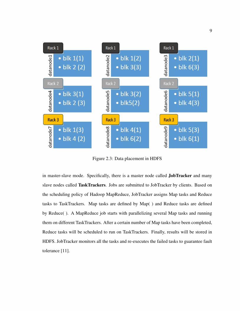
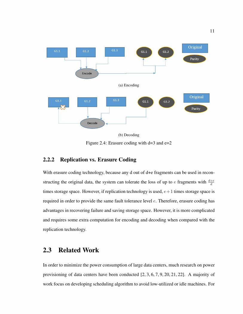
2.2.1 Erasure Coding

While replication technology provides redundancy by simply creating copies of original

data, erasure coding technology encodes the data. Specifically, given an object, erasure

coding system first divides it into d fragments, then produces another e fragments based

on generator matrix [17], and these d + e fragments are defined as an erasure coding set.

dd+e

< 1 gives the encoding rate of the set. One of the most attractive features of erasure

coding is that any d fragments in one set can be used for reconstructing the original d

fragments. To maximize fault tolerance, fragments of a set are stored in different nodes.

Figure 2.4 presents examples of encoding and decoding processes with d = 3 and e = 2.

Erasure codes are a superset of replicated and RAID systems [26]. When d = 1 and e = 2,

three replicas will be created for a block, which is the same as the replication. RAID 4

can be described as erasure coding with d = 4, e = 1, while RAID6 means e = 2. There

are several open-source erasure coding methods and libraries, like LUBY, JERASURE and

EVENODD [23].

11

(a) Encoding

(b) Decoding

Figure 2.4: Erasure coding with d=3 and e=2

2.2.2 Replication vs. Erasure Coding

With erasure coding technology, because any d out of d+e fragments can be used in recon-

structing the original data, the system can tolerate the loss of up to e fragments with d+ed

times storage space. However, if replication technology is used, e+1 times storage space is

required in order to provide the same fault tolerance level e. Therefore, erasure coding has

advantages in recovering failure and saving storage space. However, it is more complicated

and requires some extra computation for encoding and decoding when compared with the

replication technology.

2.3 Related Work

In order to minimize the power consumption of large data centers, much research on power

provisioning of data centers have been conducted [2, 3, 6, 7, 9, 20, 21, 22]. A majority of

work focus on developing scheduling algorithm to avoid low-utilized or idle machines. For

12

example, [13] proposes a dynamic provisioning and scheduling algorithm that continually

adjusts the number of active machines based on workload, and [20] develops an energy-

conserving approach where the entire system transits rapidly between a high-performance

active state and a near-zero-power idle state according to the instantaneous load.

Similar to traditional clusters, Hadoop clusters consume a plenty of energy for main-

taining low-utilized or idle machines. But due to the complexity of Hadoop clusters, fewer

research work on their power management have been published. Lang and Patel [15] de-

velop a technique called All-In Strategy(AIS) which uses all the nodes in the cluster to run

a workload and then turns off the entire cluster. However, running a workload in all Datan-

odes imposes unnecessary but significant data transfer. Besides, right workload may not

have enough tasks to run on all Datanodes simultaneously. Thus, this technique is ineffi-

cient. A more interesting research, in our opinion, is by Leverich et al. [16] who develop a

mechanism named “covering subset”. Basically, the nodes in a Hadoop cluster are grouped

into two sets, covering subset and non-covering subset. Covering subset stores at least one

replica of all data blocks such that nodes in non-covering subset can be turned off without

affecting data integrity. However, they do not consider the data availability problem caused

by node failure in covering subset. Our work adopts a concept similar to the “covering

subset” and targets at the energy efficient failure recovery in that set.

Erasure coding technology is considered as an significant approach for maintaining data

redundancy. And it is being applied to several well-known distributed storage systems [14]

such as OceanStore [14] and HyFS [18]. Weatherspoon and Kubiatowicz [26] compare

erasure coding versus replication in a quantitative way when building a distributed storage

infrastructure. Specifically, they show that erasure coding based systems have a much larger

mean time to failure than replication based systems with similar storage and bandwidth

requirements. They also point out that erasure coding systems use much less bandwidth

and storage to provide similar system durability as replication based systems.

13

The most closely related work to our thesis is [5]. In that paper, Fan et al. intro-

duce DiskReduce which integrates RAID schemes into HDFS. Because they find most data

accesses happen a short time after one block’s creation, DiskReduce proposes a delayed

encoding strategy which uses replication mechanism initially but then gradually converts

the copies into erasure coded data. Unlike our objective of achieving energy efficient fail-

ure recovery, DiskReduce employs erasure coding to save storage space for data-intensive

computing.

14

Chapter 3

Problem Setting

In this Chapter, we describe the system model and the research problem. Specifically, we

define the terms in our work including Fundamental Set (FS), Extended Set (ES), and

Waiting Set (WS).

3.1 System Model

We assume a homogenous Hadoop cluster, which is composed of a Namenode and a few

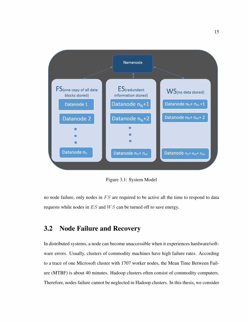
Datanodes. As depicted in Figure 3.1, the Datanodes are grouped into three sets: Funda-

mental Set (FS), Extended Set (ES), and Waiting Set (WS). FS is similar to the covering

subset (CS) defined in [16] which stores only one copy of all data blocks. Redundant data

blocks are generated following a redundancy mechanism, and they are stored in ES nodes.

The size of ES, i.e., the number of Datanodes contained in ES, is proportional to that of

FS and we store approximately the same number of blocks in each node of FS and ES.

This is because a same amount of redundancy is maintained for every unique block. Datan-

odes in WS are not assigned to store any data and they are used as backup nodes for failure

recovery. The size of WS is flexible and will not be discussed in this thesis. When there is

15

Figure 3.1: System Model

no node failure, only nodes in FS are required to be active all the time to respond to data

requests while nodes in ES and WS can be turned off to save energy.

3.2 Node Failure and Recovery

In distributed systems, a node can become unaccessible when it experiences hardware/soft-

ware errors. Usually, clusters of commodity machines have high failure rates. According

to a trace of one Microsoft cluster with 1707 worker nodes, the Mean Time Between Fail-

ure (MTBF) is about 40 minutes. Hadoop clusters often consist of commodity computers.

Therefore, nodes failure cannot be neglected in Hadoop clusters. In this thesis, we consider

16

node crash failure happened in FS. In particular, we are interest in single node failure1

since it contributes up to 90% of nodes failure in typical commodity clusters [?]. As men-

tioned, only one replica of all data blocks are stored in FS. When a FS node fails, data

integrity is damaged. To restore the data availability, we activate a new node from WS to

replace the failed node in FS. Specifically, we recover the lost data replicas by utilizing

the redundant data stored in ES, and copy them to the newly activated WS node, which

will then be moved to FS.

1Note that the failure recovery algorithms presented in Chapter 4 can be applied to recover multi-nodefailure, but the energy model we built in Chapter 5 is more towards single node failure.

17

Chapter 4

Failure Recovery Algorithms

As mentioned, node failures are common in large clusters. However, this problem has not

been considered seriously when the covering subset mechanism was designed [16]. The

system simply activates all nodes in non-covering subset to recover node failures. Since the

process of starting up and turning off machines consumes high energy and causes wear and

tear, this approach is definitely not optimal. In this thesis, we investigate and develop some

energy efficient methods for restoring lost data. First and foremost, we develop a greedy

failure recovery algorithm for the default replication-based Hadoop system to minimize

the number of nodes to be activated in ES. Then, we integrate erasure coding technology

into Hadoop to leverage its space-saving feature and to take advantage of its flexibility in

failure recovery. A greedy failure recovery algorithm for this modified Hadoop system

is developed as well. Finally, based on the analysis of these two algorithms, we design

a recovery aware placement strategy which can further improve the energy efficiency of

failure recovery.

18

4.1 Failure Recovery with Replication Based Extended

Set

By default, in HDFS, replication approach is used for maintaining data redundancy. Ac-

cordingly, we first study the case where r copies of all data blocks are stored in ES nodes.

As mentioned, we divide all the Datanodes into three sets, FS, ES, and WS, and the size

of ES is proportional to that of FS. If a total number of m unique data blocks are stored

in n FS nodes, then r ∗m data blocks are maintained in r ∗ n ES nodes. In both FS and

ES, data blocks are randomly distributed and stored and replicas of a data block are kept

in different nodes. Thus, on average, a FS/ES node gets around k = mn

data blocks.

When there is a FS node failure, only partial rather than all data blocks get lost. To

restore a few blocks, it is unnecessary to activate all Datanodes in ES. In order to achieve

an energy-efficient failure recovery, we desire to minimize the number of nodes to be turned

on during the recovery process. This energy-efficient failure recovery reduces to the set

covering problem because we need to identify the smallest number of sets (i.e., sets of data

blocks in nodes) whose union contains all lost data blocks. Since the set covering problem

is NP-hard, we develop a greedy algorithm to solve it. With this greedy failure recovery

algorithm, one replica of each lost data block will be found and sent to a newly activated

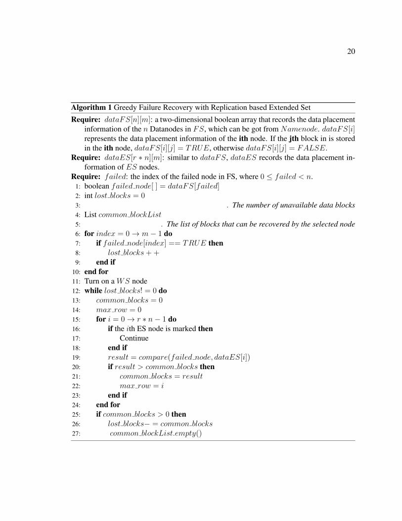
WS node for restoration. Algorithm 1 shows the details of the energy-efficient failure

recovery algorithm when we employ replication as the redundancy technique in Extended

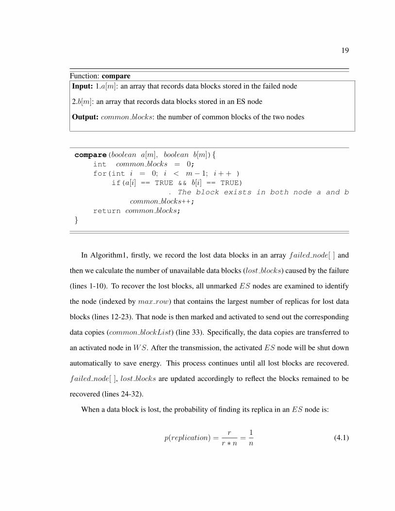
Set. The algorithm uses a “compare” function to identify common blocks shared by two

nodes. The compare function is as follows:

19

Function: compareInput: 1.a[m]: an array that records data blocks stored in the failed node

2.b[m]: an array that records data blocks stored in an ES node

Output: common blocks: the number of common blocks of the two nodes

compare(boolean a[m], boolean b[m]){int common blocks = 0;for(int i = 0; i < m− 1; i++ )

if(a[i] == TRUE && b[i] == TRUE). The block exists in both node a and b

common blocks++;return common blocks;

}

In Algorithm1, firstly, we record the lost data blocks in an array failed node[ ] and

then we calculate the number of unavailable data blocks (lost blocks) caused by the failure

(lines 1-10). To recover the lost blocks, all unmarked ES nodes are examined to identify

the node (indexed by max row) that contains the largest number of replicas for lost data

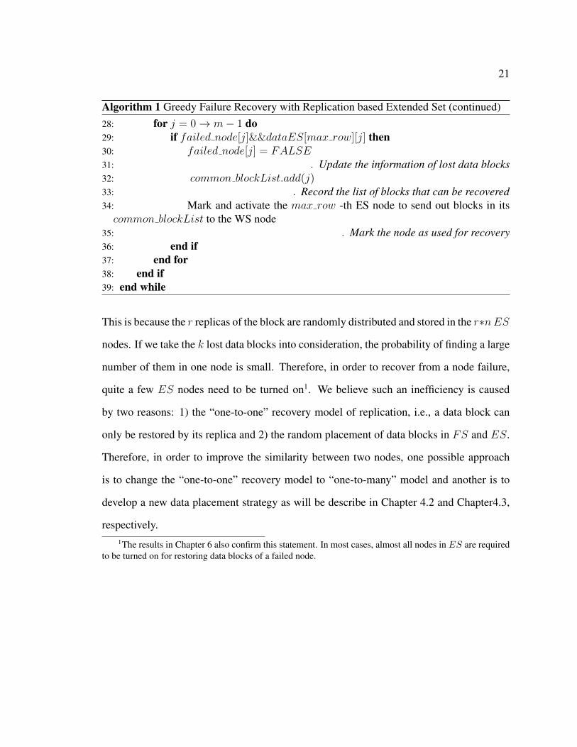
blocks (lines 12-23). That node is then marked and activated to send out the corresponding

data copies (common blockList) (line 33). Specifically, the data copies are transferred to

an activated node in WS. After the transmission, the activated ES node will be shut down

automatically to save energy. This process continues until all lost blocks are recovered.

failed node[ ], lost blocks are updated accordingly to reflect the blocks remained to be

recovered (lines 24-32).

When a data block is lost, the probability of finding its replica in an ES node is:

p(replication) =r

r ∗ n=

1

n(4.1)

20

Algorithm 1 Greedy Failure Recovery with Replication based Extended Set

Require: dataFS[n][m]: a two-dimensional boolean array that records the data placementinformation of the n Datanodes in FS, which can be got from Namenode. dataFS[i]represents the data placement information of the ith node. If the jth block in is storedin the ith node, dataFS[i][j] = TRUE, otherwise dataFS[i][j] = FALSE.

Require: dataES[r ∗ n][m]: similar to dataFS, dataES records the data placement in-formation of ES nodes.

Require: failed: the index of the failed node in FS, where 0 ≤ failed < n.1: boolean failed node[ ] = dataFS[failed]2: int lost blocks = 03: . The number of unavailable data blocks4: List common blockList5: . The list of blocks that can be recovered by the selected node6: for index = 0→ m− 1 do7: if failed node[index] == TRUE then8: lost blocks++9: end if

10: end for11: Turn on a WS node12: while lost blocks! = 0 do13: common blocks = 014: max row = 015: for i = 0→ r ∗ n− 1 do16: if the ith ES node is marked then17: Continue18: end if19: result = compare(failed node, dataES[i])20: if result > common blocks then21: common blocks = result22: max row = i23: end if24: end for25: if common blocks > 0 then26: lost blocks− = common blocks27: common blockList.empty()

21

Algorithm 1 Greedy Failure Recovery with Replication based Extended Set (continued)28: for j = 0→ m− 1 do29: if failed node[j]&&dataES[max row][j] then30: failed node[j] = FALSE31: . Update the information of lost data blocks32: common blockList.add(j)33: . Record the list of blocks that can be recovered34: Mark and activate the max row -th ES node to send out blocks in itscommon blockList to the WS node

35: . Mark the node as used for recovery36: end if37: end for38: end if39: end while

This is because the r replicas of the block are randomly distributed and stored in the r∗nES

nodes. If we take the k lost data blocks into consideration, the probability of finding a large

number of them in one node is small. Therefore, in order to recover from a node failure,

quite a few ES nodes need to be turned on1. We believe such an inefficiency is caused

by two reasons: 1) the “one-to-one” recovery model of replication, i.e., a data block can

only be restored by its replica and 2) the random placement of data blocks in FS and ES.

Therefore, in order to improve the similarity between two nodes, one possible approach

is to change the “one-to-one” recovery model to “one-to-many” model and another is to

develop a new data placement strategy as will be describe in Chapter 4.2 and Chapter4.3,

respectively.1The results in Chapter 6 also confirm this statement. In most cases, almost all nodes in ES are required

to be turned on for restoring data blocks of a failed node.

22

4.2 Failure Recovery with Erasure-Coding-Based

Extended Set

“One-to-many” recovery model means that a data block in ES has the ability to recover

several different data blocks in FS. Definitely, this recovery model cannot be achieved

when we use replication method for maintaining data redundancy. As described in Chapter

2.2.1, erasure coding mechanism has an outstanding flexibility in failure recovery. In an

erasure coding set, any d out of d + e fragments can be used to reconstruct the original

d fragments. Hence, we integrate erasure coding approach into ES for enhancing the

data recovery capability. In our system, files are divided into blocks and every randomly

selected d blocks will be treated as one erasure coding object2. For each erasure coding

object, e encoded blocks/fragments will be derived3. Since FS is kept online for serving

data requests, the original d blocks from all erasure coding sets are put into FS while the

encoded e blocks from all the sets are stored in ES. Similar to the replication approach, we

make an assumption that n Datanodes with m unique data blocks are contained in FS. In

addition, we assume data blocks in the range [i∗d , ((i+1)∗d−1)], i = 0, 1, · · · , s−1 are

grouped into the ith erasure coding object. Hence, in total, we have s = dmde erasure coding

objects and sets4. Based on an encoding rate dd+e

, e ∗ dmde number of encoded blocks are

stored in e*dnde ES nodes. In both FS and ES, all blocks are randomly distributed while

satisfying the following requirement: blocks of the same erasure coding set are stored in

different nodes. Again, each node in FS and ES stores k = mn

blockson average.2Specifically, in our system, blocks of all files are put together and then divided into erasure coding object

to reduce the unnecessary padding.3In the rest of this thesis, “block” and “fragment” have the same meaning when we refer to the “erasure

coding method” and they will be used interchangeably.4In practice, we will set lim d× s→ m+ to avoid unnecessary padding.

23

Basically, when a FS node fails, for each lost block, we need to find one encoded block

in ES and other remaining d−1 original blocks to reconstruct the data5. The reconstructed

data block will then be sent to a newly activated WS node. Specifically, approximately

k blocks from k sets are lost when a node fails. Therefore, k erasure coding sets are

required to be decoded for reconstructing the lost blocks. As described in [26], decoding

an erasure coding set is computation-intensive and time-consuming. Because all Datanodes

stop serving data requests till all lost blocks are recovered, it is obviously non-optimal to

launch all the decoding tasks on one node. To be efficient, we parallelize the k decoding

tasks on the n−1 remaining nodes of FS. That is, each FS node is assigned approximately

kn−1

decoding tasks. Since each set still has d− 1 data blocks stored in FS, to reduce data

transfer, a FS node with a block for a set will be chosen for reconstructing the set6. And

the encoded blocks in ES will also be sent to the corresponding FS node. Similar to

replication-based system, activating all ES Datanodes is unnecessary. To save energy, we

also try to minimize the number of ES nodes to be activated during the recovery process.

And this problem reduces to the set covering problem as well. In this setting, we need to

identify the smallest number of sets (i.e., sets of erasure coding sets in nodes) whose union

contains all lost erasure coding sets. Accordingly, a greedy failure recovery algorithm is

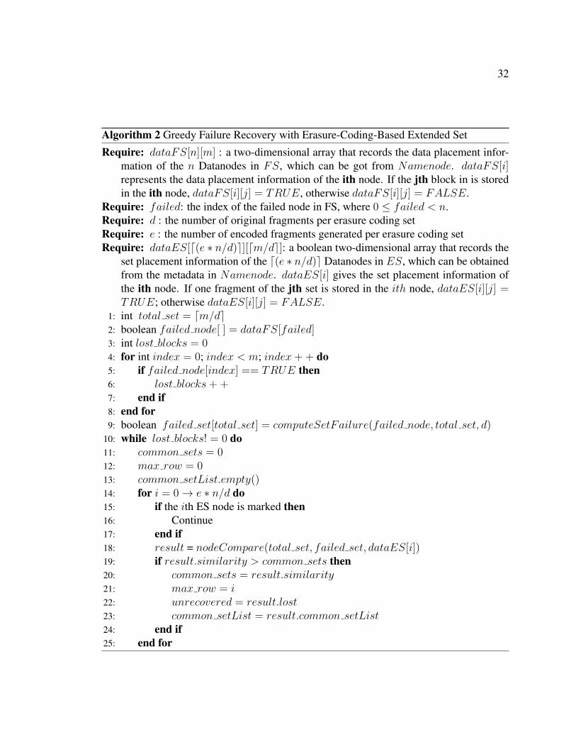
proposed. Algorithm 2 presents how our greedy algorithm works by using ES nodes to

recover a FS node failure.

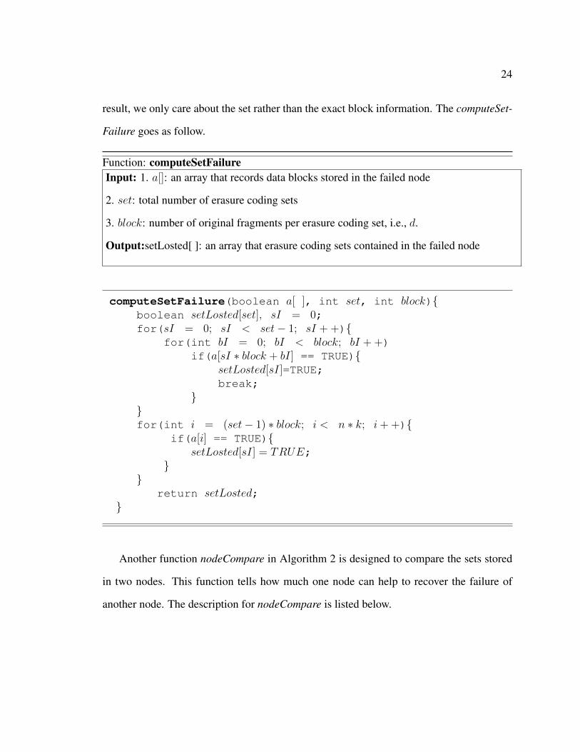
The purpose of function computeSetFailure in Algorithm 2 is to identify the sets af-

fected by the failure of a given FS node. Because with erasure coding approach, every

block in the same set can be treated equally from the perspective of failure recovery. As a5Because at most one block from one set can be stored in a node, a set can lost at most one block when a

node fails. That is, d− 1 original blocks are still available in FS6Specifically, with the random distribution of data blocks in FS, each node is likely to hold k∗(d−1)

n−1blocks for the failed sets

24

result, we only care about the set rather than the exact block information. The computeSet-

Failure goes as follow.

Function: computeSetFailureInput: 1. a[]: an array that records data blocks stored in the failed node

2. set: total number of erasure coding sets

3. block: number of original fragments per erasure coding set, i.e., d.

Output:setLosted[ ]: an array that erasure coding sets contained in the failed node

computeSetFailure(boolean a[ ], int set, int block){boolean setLosted[set], sI = 0;for(sI = 0; sI < set− 1; sI ++){

for(int bI = 0; bI < block; bI ++)if(a[sI ∗ block + bI] == TRUE){

setLosted[sI]=TRUE;break;

}}for(int i = (set− 1) ∗ block; i < n ∗ k; i++){

if(a[i] == TRUE){setLosted[sI] = TRUE;

}}

return setLosted;}

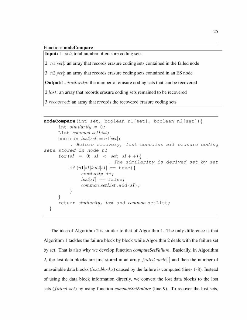
Another function nodeCompare in Algorithm 2 is designed to compare the sets stored

in two nodes. This function tells how much one node can help to recover the failure of

another node. The description for nodeCompare is listed below.

25

Function: nodeCompareInput: 1. set: total number of erasure coding sets

2. n1[set]: an array that records erasure coding sets contained in the failed node

3. n2[set]: an array that records erasure coding sets contained in an ES node

Output:1.similarity: the number of erasure coding sets that can be recovered

2.lost: an array that records erasure coding sets remained to be recovered

3.recovered: an array that records the recovered erasure coding sets

nodeCompare(int set, boolean n1[set], boolean n2[set]){int similarity = 0;List common setList;boolean lost[set] = n1[set];

. Before recovery, lost contains all erasure codingsets stored in node n1

for(sI = 0; sI < set; sI ++){. The similarity is derived set by set

if(n1[sI]&n2[sI] == true){similarity ++;lost[sI] == false;common setList.add(sI);

}}return similarity, lost and common setList;

}

The idea of Algorithm 2 is similar to that of Algorithm 1. The only difference is that

Algorithm 1 tackles the failure block by block while Algorithm 2 deals with the failure set

by set. That is also why we develop function computeSetFailure. Basically, in Algorithm

2, the lost data blocks are first stored in an array failed node[ ] and then the number of

unavailable data blocks (lost blocks) caused by the failure is computed (lines 1-8). Instead

of using the data block information directly, we convert the lost data blocks to the lost

sets (failed set) by using function computeSetFailure (line 9). To recover the lost sets,

26

all unmarked ES nodes are examined to identify their abilities in recovering the failure.

The node with the maximum recovery capability (indexed by max row) , that is, a node

containing the largest number of fragments for lost sets, is selected (lines 10-25). That node

is then marked and activated to send out the corresponding data blocks (common setList)

for failure recovery (line 29) and failed set[ ], lost blocks are updated accordingly to

reflect the sets remained to be recovered (lines 26-31). Specifically, the blocks are sent to

the n− 1 remaining FS nodes. After the transmission, the activated ES node will be shut

down automatically.

Besides an encoded block retrieved from an ES node and a local block, to decode

an erasure coding set, a FS node still needs to get d − 2 original blocks from other FS

nodes. Note that a decoding task can only be started after d blocks of a set have been

received. Therefore, we transfer data blocks following their set order. Since decoding

is computation-intensive and data transfer is network-intensive, to be efficient, we launch

them simultaneously whenever possible. After all lost sets are decoded, the reconstructed

data blocks will be sent to a newly activated WS node.

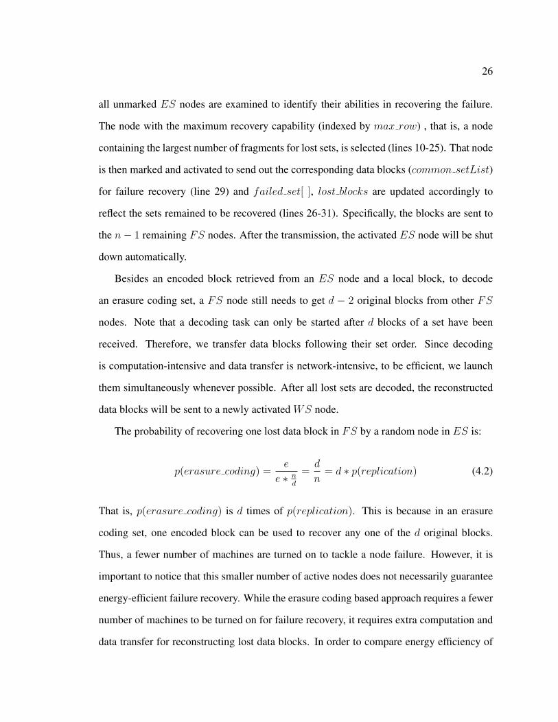
The probability of recovering one lost data block in FS by a random node in ES is:

p(erasure coding) =e

e ∗ nd

=d

n= d ∗ p(replication) (4.2)

That is, p(erasure coding) is d times of p(replication). This is because in an erasure

coding set, one encoded block can be used to recover any one of the d original blocks.

Thus, a fewer number of machines are turned on to tackle a node failure. However, it is

important to notice that this smaller number of active nodes does not necessarily guarantee

energy-efficient failure recovery. While the erasure coding based approach requires a fewer

number of machines to be turned on for failure recovery, it requires extra computation and

data transfer for reconstructing lost data blocks. In order to compare energy efficiency of

27

failure recovery in these two systems, we build energy model and give analysis in Chapter

5.

4.3 Recovery Aware Data Placement Strategy

The incentive of the greedy failure recovery algorithms is to minimize the number of nodes

required to be activated during the recovery process. However, the simulation results7

show that the greedy algorithms are inefficient and a large proportion of machines are

always required in order to recover a FS node failure. Basically, more than 1r

of ES nodes

are demanded when we use replication-based system, and more than 1e

of ES nodes are

required if erasure-coding-based system is employed. Mathematic analysis also justifies

and proves the correctness of the simulation results. Specifically, when erasure-coding-

based ES is used, approximately k blocks from k sets are lost if a FS node fails. Suppose

f(x) data blocks can be recovered in the xth (x > 0) attempt by applying the greedy failure

recovery algorithm (refer to Chapter 4.2, based on the definition of greedy algorithm, we

have f(x) ≥ f(x+ 1) > 0. For a given failure, we define the number of sets recovered by

an ES node as its recovery capability. Hence, f(x) also represents the recovery capability

of the node used by the greedy algorithm in the xth iteration. Assume F (p) =p∑

i=1

f(i), in

which p ≥ 1 and F (0) = 0, and if a total of X steps are required to deal with a node failure,

F (X) = k. As a characteristic of greedy algorithm, solution at each step is at least as good

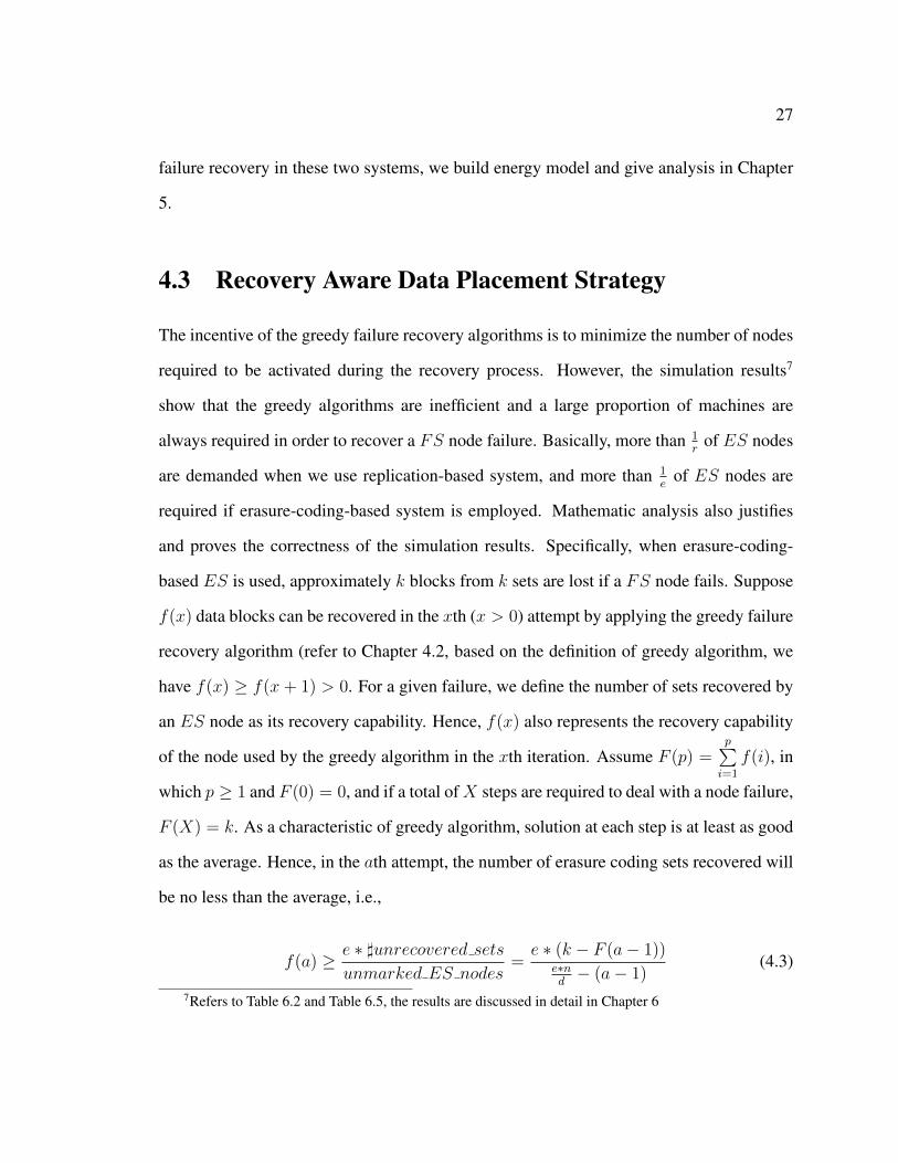
as the average. Hence, in the ath attempt, the number of erasure coding sets recovered will

be no less than the average, i.e.,

f(a) ≥ e ∗ ]unrecovered sets

unmarked ES nodes=

e ∗ (k − F (a− 1))e∗nd− (a− 1)

(4.3)

7Refers to Table 6.2 and Table 6.5, the results are discussed in detail in Chapter 6

28

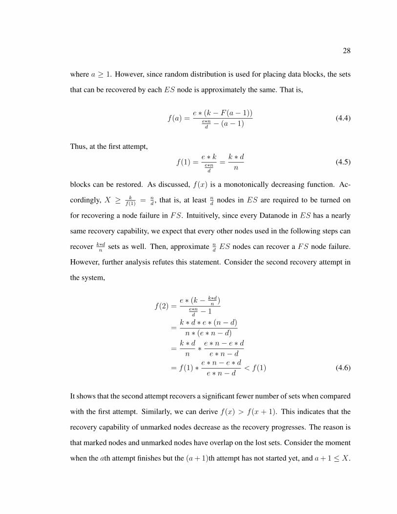
where a ≥ 1. However, since random distribution is used for placing data blocks, the sets

that can be recovered by each ES node is approximately the same. That is,

f(a) =e ∗ (k − F (a− 1))

e∗nd− (a− 1)

(4.4)

Thus, at the first attempt,

f(1) =e ∗ ke∗nd

=k ∗ dn

(4.5)

blocks can be restored. As discussed, f(x) is a monotonically decreasing function. Ac-

cordingly, X ≥ kf(1)

= nd, that is, at least n

dnodes in ES are required to be turned on

for recovering a node failure in FS. Intuitively, since every Datanode in ES has a nearly

same recovery capability, we expect that every other nodes used in the following steps can

recover k∗dn

sets as well. Then, approximate ndES nodes can recover a FS node failure.

However, further analysis refutes this statement. Consider the second recovery attempt in

the system,

f(2) =e ∗ (k − k∗d

n)

e∗nd− 1

=k ∗ d ∗ e ∗ (n− d)

n ∗ (e ∗ n− d)

=k ∗ dn∗ e ∗ n− e ∗ d

e ∗ n− d

= f(1) ∗ e ∗ n− e ∗ de ∗ n− d

< f(1) (4.6)

It shows that the second attempt recovers a significant fewer number of sets when compared

with the first attempt. Similarly, we can derive f(x) > f(x + 1). This indicates that the

recovery capability of unmarked nodes decrease as the recovery progresses. The reason is

that marked nodes and unmarked nodes have overlap on the lost sets. Consider the moment

when the ath attempt finishes but the (a+ 1)th attempt has not started yet, and a+ 1 ≤ X .

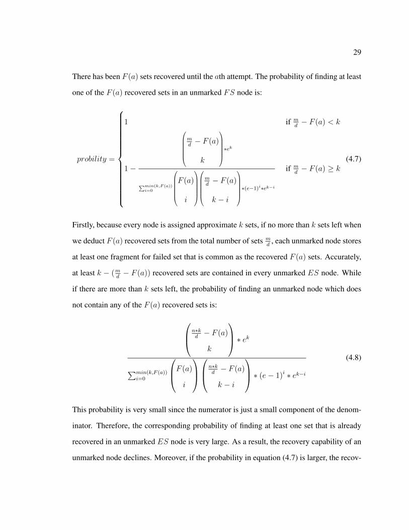
29

There has been F (a) sets recovered until the ath attempt. The probability of finding at least

one of the F (a) recovered sets in an unmarked FS node is:

probility =

1 if md− F (a) < k

1−

md− F (a)

k

∗ek

∑min(k,F (a))i=0

F (a)

i

md− F (a)

k − i

∗(e−1)i∗ek−i

if md− F (a) ≥ k

(4.7)

Firstly, because every node is assigned approximate k sets, if no more than k sets left when

we deduct F (a) recovered sets from the total number of sets md

, each unmarked node stores

at least one fragment for failed set that is common as the recovered F (a) sets. Accurately,

at least k − (md− F (a)) recovered sets are contained in every unmarked ES node. While

if there are more than k sets left, the probability of finding an unmarked node which does

not contain any of the F (a) recovered sets is:

n∗kd− F (a)

k

∗ ek∑min(k,F (a))

i=0

F (a)

i

n∗k

d− F (a)

k − i

∗ (e− 1)i ∗ ek−i

(4.8)

This probability is very small since the numerator is just a small component of the denom-

inator. Therefore, the corresponding probability of finding at least one set that is already

recovered in an unmarked ES node is very large. As a result, the recovery capability of an

unmarked node declines. Moreover, if the probability in equation (4.7) is larger, the recov-

30

ery capability of an unmarked node is likely to decrease more sharply. Hence, the inherent

similarity of any two ES nodes largely harms the efficiency of the greedy algorithm.

When a FS node fails, approximately k blocks from k sets are lost. Ideally, we expect

that the algorithm could select X nodes with non-overlapping sets. That is, the X selected

nodes contain only one fragment for each failed set. However, this objective is nontrivial

because the specific sets involved in a failure are unpredictable. N node fails randomly and

any k out of md

sets could get lost. Fortunately, only one fragment per set is lost when a node

fails. Accordingly, a collection that contains one fragment for each set can be regarded as

the covering set for a node failure. Thus, we group one fragment from every set together

to form a unit. Specifically, we divide ES nodes into e equal partitions. Each set stores

one fragment in a partition. Hence, the lost k sets can be found in any of the e partitions

while any two ES nodes in a partition do not have any overlapping sets. In the worst

case, a node failure in FS can be recovered by 1e∗ e∗n

d= n

dnumber of nodes. Therefore,

X ≤ nd. Note that replication can be treated as a special case of erasure coding where

d = 1 and e = 2. With the greedy algorithm presented in Chapter 4.1, at least n nodes are

demanded for recovering a FS node failure. To improve the efficiency, we can also apply a

similar recovery aware data placement strategy in the replication-based system. Likewise,

the replication based ES is partitioned into r parts since r replicas are maintained in ES.

One replica of each data block is stored in a partition. Therefore, at most n nodes will be

required for tackling a FS node failure.

There are also other data placement strategies that can improve the similarity between

FS and ES nodes and thus lead to a smaller number of node activation. However, they

are often too constrained to be applied. For example, in replication-based system, one in-

tuitive idea is to maintain r mirrored nodes for a FS node in ES. In other words, each ES

partition is a clone of FS. As a result, in every partition, we are able to find a mirrored

Datanode for any failed FS node. However, such a mechanism is not feasible. Specifically,

31

the data placement in FS is often changing dynamically in order to meet various require-

ments such as achieving workload balance. We need to keep ES nodes online to follow the

data placement change of FS nodes. This violates the energy saving requirement. In this

thesis, we thus have developed a much less constracined recovery-aware data placement

strategy.

32

Algorithm 2 Greedy Failure Recovery with Erasure-Coding-Based Extended Set

Require: dataFS[n][m] : a two-dimensional array that records the data placement infor-mation of the n Datanodes in FS, which can be got from Namenode. dataFS[i]represents the data placement information of the ith node. If the jth block in is storedin the ith node, dataFS[i][j] = TRUE, otherwise dataFS[i][j] = FALSE.

Require: failed: the index of the failed node in FS, where 0 ≤ failed < n.Require: d : the number of original fragments per erasure coding setRequire: e : the number of encoded fragments generated per erasure coding setRequire: dataES[d(e ∗ n/d)e][dm/de]: a boolean two-dimensional array that records the

set placement information of the d(e ∗ n/d)e Datanodes in ES, which can be obtainedfrom the metadata in Namenode. dataES[i] gives the set placement information ofthe ith node. If one fragment of the jth set is stored in the ith node, dataES[i][j] =TRUE; otherwise dataES[i][j] = FALSE.

1: int total set = dm/de2: boolean failed node[ ] = dataFS[failed]3: int lost blocks = 04: for int index = 0; index < m; index++ do5: if failed node[index] == TRUE then6: lost blocks++7: end if8: end for9: boolean failed set[total set] = computeSetFailure(failed node, total set, d)

10: while lost blocks! = 0 do11: common sets = 012: max row = 013: common setList.empty()14: for i = 0→ e ∗ n/d do15: if the ith ES node is marked then16: Continue17: end if18: result = nodeCompare(total set, failed set, dataES[i])19: if result.similarity > common sets then20: common sets = result.similarity21: max row = i22: unrecovered = result.lost23: common setList = result.common setList24: end if25: end for

33

Algorithm 2 Greedy Failure Recovery with Erasure-Coding-Based ExtendedSet(continued)26: if common sets > 0 then27: lost blocks− = common sets28: failed set = unrecovered29: Mark and activate the max row th node of ES to send out encoded fragments

in specified common setList to the corresponding FS nodes30: . Mark the node as used for recovery31: end if32: end while

34

Chapter 5

Energy Model

In this Chapter, we build the energy model for analyzing the energy requirement of failure

recovery.

Before discussing the energy consumption of the failure recovery process, it is neces-

sary to mention that we assume that the system serves data request only when all data are

available in FS. In other words, if a node fails, no data request will be served during the

failure recovery process. When a node fails in FS, based on the failure recovery algorithms

we introduced in Chapter 4, we know the set of ES machines that need to be turned on for

the failure recovery. Besides powering up these ES nodes, some extra work is required

to restore the lost data. Specifically, nodes could be involved in sending/receiving data, or

decoding data if the erasure coding approach is applied. Because we assume a homoge-

nous cluster the power consumed by any two nodes to do the same task are supposed to be

the same. In our system, possible tasks include data transfer (i.e., sending/receiving data

blocks1), decoding (i.e., reconstructing the data) and both, whose power consumption are

denoted as Ptran, Pcomp, and Pt+c, respectively. Moreover, the energy and time spent by a

node during the activation (inactivation) process is represented by Eact and Tact (Einact and1In order to simplify the analysis, we assume sending and receiving the same amount of data consume

the same amount of energy.

35

Tinact). Additionally, Pidle represents the power consumption of an idle machine. Since

our cluster consists of FS, ES and WS and the recovery process starts with retrieving

data from ES and ends with receiving data in WS, we discuss the energy consumption of

two failure recovery algorithms by analyzing energy spent in ES, FS and WS (E(ES),

E(FS), and E(WS)) during the recovery processes.

5.1 Energy spent in ES

In ES, a set of nodes derived by the failure recovery algorithms will be turned on to send

out data blocks for recovering lost data, and these nodes will be turned off immediately

after the transmission. We assume every activated node in ES spends the same amount of

energy during the recovery process. Suppose A nodes are required to be activated and each

node spends TES seconds in sending out blocks2. Then, the energy consumed in ES can

be described as:

E(ES) = A ∗ (Eact + Ptran ∗ TES + Einact) (5.1)

In formula (5.1), Eact + Ptran ∗ TES + Einact stands for the total energy consumed by an

ES node during the failure recovery.

• For replication-based system:

When replication is used in ES, the data blocks will be directly transferred from

ES nodes to a WS node. As a result, data transfer speed is limited by the receiv-

ing capability of the WS node rather than the aggregated sending capability of ES

nodes. That is, we need TES = TWS = 64∗kb

(seconds) to transfer data, where 64

(MB) is the data block size and b (MB/s) gives a machine’s network I/O bandwidth.2Subscripts SR and EC will be added when we refer to the replication-based and erasure-coding-based

systems. And this notation also applies to other parameters that will be used in this thesis.

36

Consequently, formula (5.1) becomes:

E(ES)SR = ASR ∗ (Eact + Ptran ∗64 ∗ k

b+ Einact) (5.2)

• For erasure-coding-based system:

Unlike replication-based system, in which data collected from ES can be used di-

rectly, some extra decoding work is required in the erasure-coding-based system.

In order to reconstruct an original data object, d blocks need to be retrieved for an

erasure coding set. Due to a FS node failure, we need to recover approximately

k erasure coding data objects/sets. For each set, there are still d − 1 blocks in FS

and thus one more block needs to be retrieved from an ES node. Totally, approx-

imately k blocks sent from AEC ES nodes are needed in reconstructing the k lost

data blocks. On average, an activated EC node sends out kAEC

blocks to FS nodes.

As mentioned, in order to minimize the decoding time and maximize the utilization

of active machines, we use the n − 1 FS machines to reconstruct the k sets in par-

allel. Each machine will be assigned kn−1

number of sets to reconstruct. Thus, kn−1

ES blocks are received per node in FS. If kAEC≥ k

n−1, i.e., AEC < n − 1, the data

transfer speed is limited by the aggregated sending capability of the AEC ES nodes.

That is, TES = TFS1 =64∗ k

AEC

b= 64∗k

AEC∗b (seconds)3; Otherwise, the data transfer

speed is limited by the aggregated receiving capability of n − 1 FS nodes. That is,

TES = TFS1 =64∗ k

n−1

b= 64∗k

(n−1)∗b (seconds). As a result, formula (5.1) become:

E(ES)EC = AEC ∗ (Eact + Ptran ∗64 ∗ k

min(AEC , (n− 1)) ∗ b+ Einact) (5.3)

3This is a more common situation. Since ES contains totally n ∗ ed and it is often the case that d ≥ e,

there is often less than n number of ES nodes and AEC is likely to be the less than n− 1.

37

5.2 Energy spent in FS

The energy consumed by FS nodes largely depends on the redundancy technology we

used in ES. If replication approach is employed, all active FS nodes are simply kept

idle waiting for the recovery process to complete. While if the erasure coding approach is

applied, nodes in FS are involved in data transfer and decoding, as mentioned in Chapter

4.2.

E(FS) = (n− 1) ∗ (Pidle ∗ Tidle + Etran + Et+c + Ecomp) (5.4)

where Ecomp, Et+c, and Etran stand for energy devoured by a FS node in decoding only,

data transfer and decoding in parallel, and data transfer only, respectively.

• For replication-based system:

In replication-based system, FS nodes are not involved in a failure recovery. How-

ever, they still consume energy because the n − 1 nodes are kept active during the

process. They wait for Tact+64∗kb

seconds when ES nodes are activated and data are

transferred from ES nodes to a WS node. Thus, the energy consumed by FS nodes

is:

E(FS)SR = (n− 1) ∗ (Pidle ∗ (Tact +64 ∗ k

b)) (5.5)

• For erasure-coding-based system:

It is a bit more complicated to analyze energy consumed by FS nodes in an erasure-

coding based system, since lost data blocks need to be recomputed in FS nodes.

When a FS node fails, approximately k blocks from k different erasure coding sets

are lost. To be efficient, these k sets will be reconstructed by the n − 1 FS nodes

in parallel. That is, each FS node reconstructs about kn−1

sets. Since each of the k

sets still has d − 1 blocks stored in FS nodes, to reduce data transfer, a FS node

with a block for a set will be chosen for reconstructing the set. A FS node will

38

get d − 2 blocks from other FS nodes and a block from an ES node, and then

reconstruct the set using the d blocks. To start with, blocks from ES nodes are

transferred to destination FS nodes. Specifically, a FS node first waits for pow-

ering up ES nodes and receiving data from them. It idle waits for Tact seconds,

and then spends TFS1 = 64∗kmin(AEC ,(n−1))∗b (seconds) in accepting k

n−1data blocks

from ES nodes. Hence, the energy consumption of a FS node during this stage is

Pidle ∗ Tact + Ptran ∗ 64∗kmin(AEC ,(n−1))∗b (J). In the next stage, a FS node retrieves

the d − 2 blocks from other FS nodes to decode a set. Each FS node sends and

receives approximately kn−1∗ (d− 2) number of blocks. Because the network inter-

face card (NIC) can work in full duplex nowadays, sending and receiving data can be

processed simultaneously without affecting each other. Thus, the time in transferring

data within FS is64∗ k

n−1∗(d−2)

b(seconds) in total and Ttran = 64∗(d−2)

b(seconds) per

set. As discussed in Chapter 4.2, data transfer and decoding are launched simultane-

ously whenever possible. And data blocks are transferred following their set order.

After receiving all blocks of the first erasure coding set, a FS node starts decoding

that set while receiving blocks for the second set. Suppose the decoding time is Tcomp

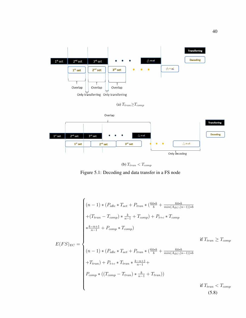
per set. There could be two scenarios as characterized in Figure 5.1.

(a) When Ttran≥Tcomp, data transfer and decoding can overlap for Tcomp∗( kn−1−1)

seconds when decoding all but the last set. A FS node spends Ttran + (Ttran−

Tcomp) ∗ ( kn−1− 1) = Tcomp + (Ttran− Tcomp) ∗ k

n−1seconds exclusively in data

transfer and Tcomp seconds exclusively in decoding. Thus, the energy consumed

39

by a FS node in this process is:

Etran + Et+c + Ecomp

= Ptran ∗ (Tcomp + (Ttran − Tcomp) ∗k

n− 1)

+ Pt+c ∗ (Tcomp ∗ (k

n− 1− 1)) + Pcomp ∗ Tcomp

(5.6)

(b) When Ttran < Tcomp, data transfer and decoding can overlap for Ttran∗( kn−1−1)

seconds when transferring all but the first set. A FS node also spends (Tcomp−

Ttran)∗( kn−1−1)+Tcomp = Ttran+(Tcomp−Ttran)∗ k

n−1seconds exclusively in

decoding and Ttran seconds exclusively in data transfer. Therefore, the energy

consumed by a FS node in this process is:

Etran + Et+c + Ecomp

= Ptran ∗ Ttran

+ Pt+c ∗ (Ttran ∗ (k

n− 1− 1))

+ Pcomp ∗ (Ttran + (Tcomp − Ttran) ∗k

n− 1)

(5.7)

After completing the decoding, the n − 1 FS nodes send reconstructed k blocks

to a WS node. The data transfer time relys on the receiving capability of the WS

node. Thus, TFS2 = TWS = 64∗kb

seconds. The energy cost during this period is:

Ptran ∗ 64∗kb

.

Eventually, we expand the formula (5.4) as follow:

40

(a) Ttran≥Tcomp

(b) Ttran < Tcomp

Figure 5.1: Decoding and data transfer in a FS node

E(FS)EC =

(n− 1) ∗ (Pidle ∗ Tact + Ptran ∗ (64∗kb + 64∗kmin(AEC ,(n−1))∗b

+(Ttran − Tcomp) ∗ kn−1

+ Tcomp) + Pt+c ∗ Tcomp

∗k−n+1n−1

+ Pcomp ∗ Tcomp)

if Ttran ≥ Tcomp

(n− 1) ∗ (Pidle ∗ Tact + Ptran ∗ (64∗kb + 64∗kmin(AEC ,(n−1))∗b

+Ttran) + Pt+c ∗ Ttran ∗ k−n+1n−1

+

Pcomp ∗ ((Tcomp − Ttran) ∗ kn−1

+ Ttran))

if Ttran < Tcomp

(5.8)

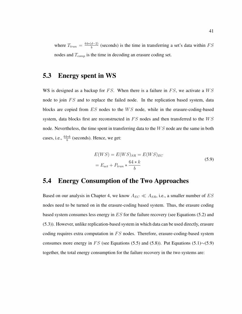
41

where Ttran = 64∗(d−2)b

(seconds) is the time in transferring a set’s data within FS

nodes and Tcomp is the time in decoding an erasure coding set.

5.3 Energy spent in WS

WS is designed as a backup for FS. When there is a failure in FS, we activate a WS

node to join FS and to replace the failed node. In the replication based system, data

blocks are copied from ES nodes to the WS node, while in the erasure-coding-based

system, data blocks first are reconstructed in FS nodes and then transferred to the WS

node. Nevertheless, the time spent in transferring data to the WS node are the same in both

cases, i.e., 64∗kb

(seconds). Hence, we get:

E(WS) = E(WS)SR = E(WS)EC

= Eact + Ptran ∗64 ∗ k

b

(5.9)

5.4 Energy Consumption of the Two Approaches

Based on our analysis in Chapter 4, we know AEC � ASR, i.e., a smaller number of ES

nodes need to be turned on in the erasure-coding based system. Thus, the erasure coding

based system consumes less energy in ES for the failure recovery (see Equations (5.2) and

(5.3)). However, unlike replication-based system in which data can be used directly, erasure

coding requires extra computation in FS nodes. Therefore, erasure-coding-based system

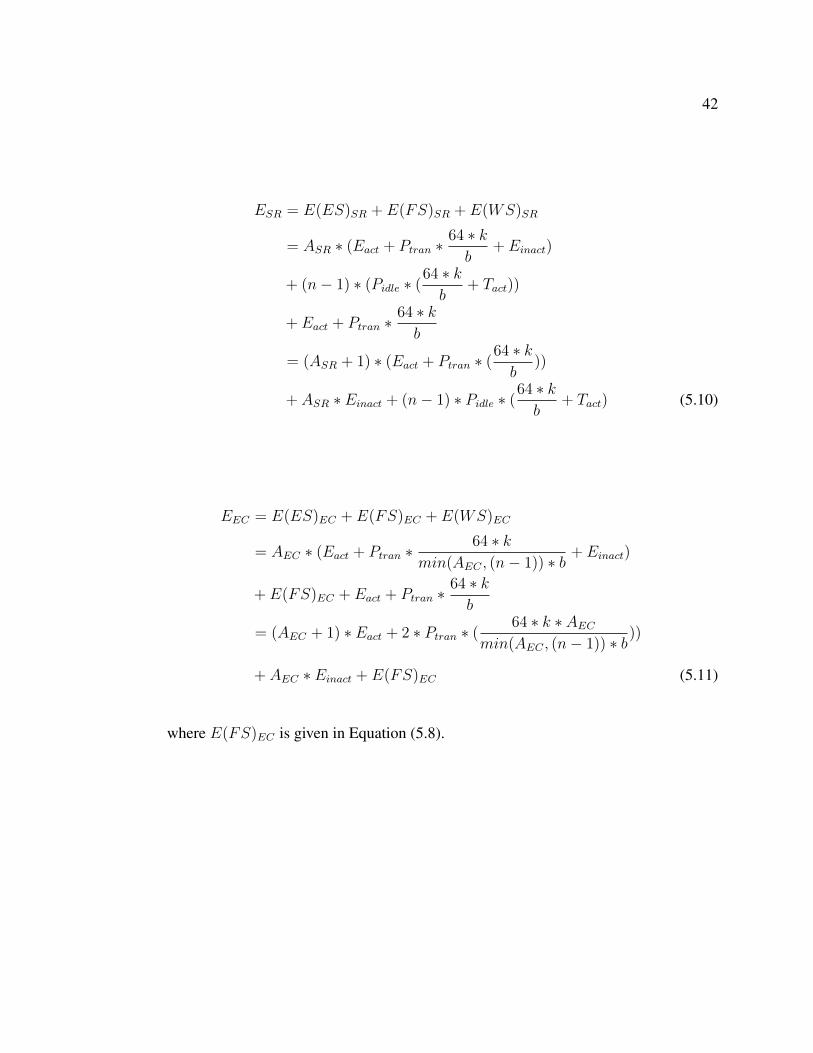
consumes more energy in FS (see Equations (5.5) and (5.8)). Put Equations (5.1)∼(5.9)

together, the total energy consumption for the failure recovery in the two systems are:

42

ESR = E(ES)SR + E(FS)SR + E(WS)SR

= ASR ∗ (Eact + Ptran ∗64 ∗ k

b+ Einact)

+ (n− 1) ∗ (Pidle ∗ (64 ∗ k

b+ Tact))

+ Eact + Ptran ∗64 ∗ k

b

= (ASR + 1) ∗ (Eact + Ptran ∗ (64 ∗ k

b))

+ ASR ∗ Einact + (n− 1) ∗ Pidle ∗ (64 ∗ k

b+ Tact) (5.10)

EEC = E(ES)EC + E(FS)EC + E(WS)EC

= AEC ∗ (Eact + Ptran ∗64 ∗ k

min(AEC , (n− 1)) ∗ b+ Einact)

+ E(FS)EC + Eact + Ptran ∗64 ∗ k

b

= (AEC + 1) ∗ Eact + 2 ∗ Ptran ∗ (64 ∗ k ∗ AEC

min(AEC , (n− 1)) ∗ b))

+ AEC ∗ Einact + E(FS)EC (5.11)

where E(FS)EC is given in Equation (5.8).

43

Chapter 6

Simulation

In this chapter, we compare the replication-based recovery algorithm with the erasure-

coding-based recovery algorithm via simulating a node failure in FS. We profile our local

cluster, Bugeater2, to estimate the energy consumption of the two methods with/without

our recovery aware data placement strategy plugged in.

6.1 Energy consumption

In Chapter 5, we analyzed and modeled the energy consumption for failure recovery. To get

the parameters for the model and estimate the energy cost, we use and profile our testbed

cluster, Bugeater2. In Bugeater2, every node has two AMD Opteron(tm) Processors 248

(2.2GHz, 64bit), 4GB Memory and one 80GB SATA disk. The speed of the switch that

connects these nodes is 1Gbps. We use a Server Tech CWG-CDU power distribution unit

(PDU) to measure the energy consumption. The energy consumed to boot up a machine is

24650Joule, that is, Eact = 24650J , while the energy consumed to shut down a machine

is very small and can be ignored, hence, we set Einact = 0J . When a machine is idle, it

consumes 70J per second, i.e., Pidle = 70J/s while it consumes 90J per second if the

44

machine is busy in decoding, that is, Pcomp = 90J/s. Based on our measurements, the

extra energy consumed in data transfer is negligible. Thus, we set Ptran = Pidle = 70J/s

and Pt+c = Pcomp = 90J/s. The time spent in activating a machine in Bugeater2 is about

30 seconds, i.e. Tact = 30s. Moreover, although the ethernet is supposed to be 1Gbps

= 128MB/s, but only 35MB/s can be achieved in practice. Thus, we set b = 35MB/s.

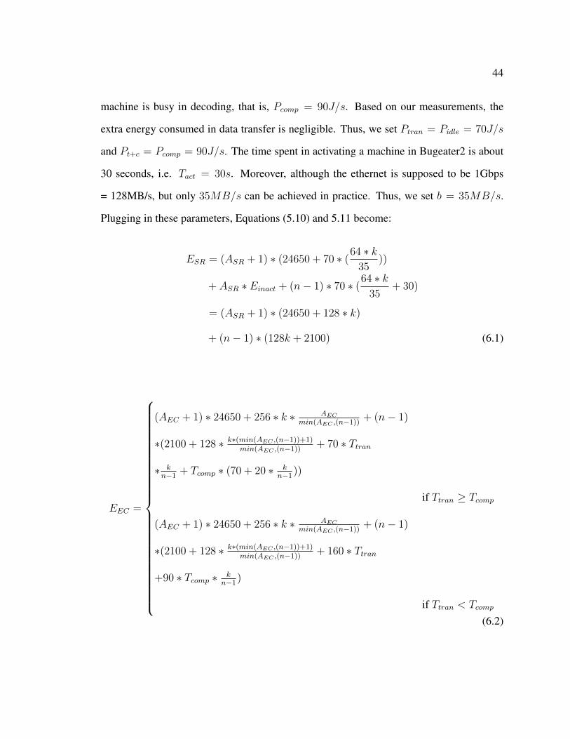
Plugging in these parameters, Equations (5.10) and 5.11 become:

ESR = (ASR + 1) ∗ (24650 + 70 ∗ (64 ∗ k35

))

+ ASR ∗ Einact + (n− 1) ∗ 70 ∗ (64 ∗ k35

+ 30)

= (ASR + 1) ∗ (24650 + 128 ∗ k)

+ (n− 1) ∗ (128k + 2100) (6.1)

EEC =

(AEC + 1) ∗ 24650 + 256 ∗ k ∗ AEC

min(AEC ,(n−1))+ (n− 1)

∗(2100 + 128 ∗ k∗(min(AEC ,(n−1))+1)min(AEC ,(n−1))

+ 70 ∗ Ttran

∗ kn−1

+ Tcomp ∗ (70 + 20 ∗ kn−1

))

if Ttran ≥ Tcomp

(AEC + 1) ∗ 24650 + 256 ∗ k ∗ AEC

min(AEC ,(n−1))+ (n− 1)

∗(2100 + 128 ∗ k∗(min(AEC ,(n−1))+1)min(AEC ,(n−1))

+ 160 ∗ Ttran

+90 ∗ Tcomp ∗ kn−1

)

if Ttran < Tcomp

(6.2)

45

6.2 Simulation Results

To compare the replication-based system with the erasure-coding-based system, we con-

sider two situations: 1) same fault tolerance level and 2) same storage space. In both situa-

tions, we always use Hadoop’s default replication factor, 3, i.e., r = 2, for the replication-

based system. Additionally, the block size is set at 64MB by default and n∗20GB data will

be randomly distributed in FS, that is, about k = 20GB/64MB = 320 blocks per node.

Based on the performance comparison of different erasure coding libraries in [23], we em-

ploy Jerasure erasure coding in our system. Moreover, we simulate clusters of different

sizes ranging from 14 nodes to 290 nodes, and every cluster is divided into FS, ES and

WS. Basically, 2 nodes are put into WS as backups, and one third of the remaining nodes

are treated as FS nodes. Hence, we have 14−23

= 4 FS nodes in the smallest cluster while

290−23

= 96 FS nodes in the largest cluster, i.e., n ranges from 4 nodes to 96 nodes. As

described in Chapter 4, the number of nodes in ES depends on the redundancy mechanism.

If replication approach is used, we have r∗n = 2∗n nodes in ES, that is, all the remaining

nodes of a cluster. While if erasure coding based approach is used, e ∗ nd

nodes is contained

in ES.

• Same Fault Tolerance Level

In order to compute the total energy consumption spent in erasure-coding-based sys-

tem, we still need to know the amount of time spent for decoding an erasure coding

set, i.e., Tcomp. According to the erasure coding algorithm mechanism, when the frag-

ment size is fixed, the decoding time of a set depends on its size and encoding rate,

i.e., d and dd+e

. When we consider the same fault tolerance level, i.e., e = r = 2. Ta-

ble 6.1 presents the corresponding decoding time on a node as the set size d changes1.1If the computing capability of a node that executes decoding tasks is fixed, a quadratic model can be

built to estimate the decoding time of an erasure coding set for given d and e.

46

Table 6.1: Time spent by Jerasure’s erasure coding (e = 2)

blocks per set (d+ e) encoding rate ( dd+e

) Decoding time (s)

5 35

0.514

6 46

0.756

7 57

0.874

8 68

1.086

10 810

1.754

12 1012

2.889

14 1214

3.98

18 1618

6.442

22 2022

10.598

26 2426

16.363

In order to calculate ESR and EEC , according to Equation (6.1) and (6.2), the number

of machines in ES to be activated, i.e., ASR and AEC , should be derived. Basically,

given a cluster, we simulate a random node failure 10 times and use the average value

of these experiments as an estimation of ASR and AEC . Table 6.2 shows the corre-

sponding ASR and AEC when handling a node failure in FS. The resultant energy

consumptions are also presented in Table 6.2. While n stands for the number of nodes

in FS, n(ES)EC gives the number of nodes in ES when erasure coding mechanism

is applied2. n(ES)EC = e∗n/d = 2∗n/d. As Table 6.2 shows, a much fewer number

of ES nodes need to be activated when we adopt the erasure-coding-based ES. As

indicated by ESR

EEC, the corresponding energy consumption is also smaller with 1.87

as the average value. Figure 6.1 shows the energy saving advantages of erasure-

coding-based system as cluster size increases3. Besides, as another major benefit of

erasure coding, storage space can be saved while maintaining the same level of fault2While not given explicitly in the table, the number of nodes in FS is always r ∗ n = 2 ∗ n when

replication method is used.3Note that, in Figures 6.1 - 6.6, given a cluster, we use the lowest energy consumption EEC (which

is achieved with an optimal setting of d) of the erasure-coding-based system. This is because based on the

47

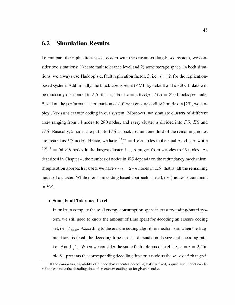
Figure 6.1: Comparison on energy consumption of replication-based system vserasure-coding-based system (same fault tolerance level)

tolerance. Specifically, if we store the same amount of data in FS, i.e., the same

number of unique data blocks in the cluster, the total number of nodes needed for

erasure-coding-based ES is much less than that for replication-based ES.

After comparing the two algorithms without the recovery aware data placement strat-

egy enabled, we carry out the simulations by enabling the recovery aware data place-

ment strategy in the algorithms. Table 6.3 presents the results with the recovery aware

data placement strategy plugged in. As we expected, Table 6.2 and Table 6.3 show

that a fewer number of machines are activated when recovering a single node failure

in a cluster when we adopt the recovery aware data placement strategy. In general,

the erasure-coding-based system still consumes less energy in failure recovery with

1.52 as the average value of ESR

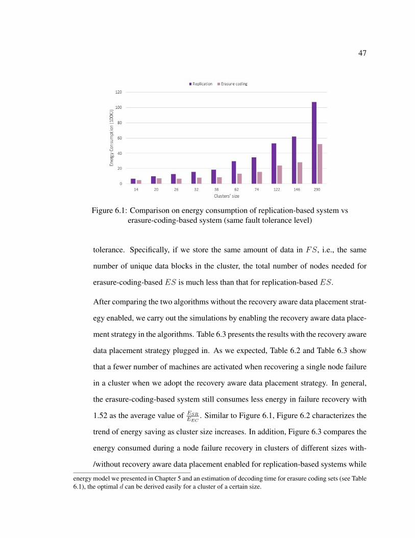
EEC. Similar to Figure 6.1, Figure 6.2 characterizes the

trend of energy saving as cluster size increases. In addition, Figure 6.3 compares the

energy consumed during a node failure recovery in clusters of different sizes with-

/without recovery aware data placement enabled for replication-based systems while

energy model we presented in Chapter 5 and an estimation of decoding time for erasure coding sets (see Table6.1), the optimal d can be derived easily for a cluster of a certain size.

48

Figure 6.4 compares that for erasure-coding-based systems. With recovery aware

data placement strategy, a fewer number of ES machines are required to be activated

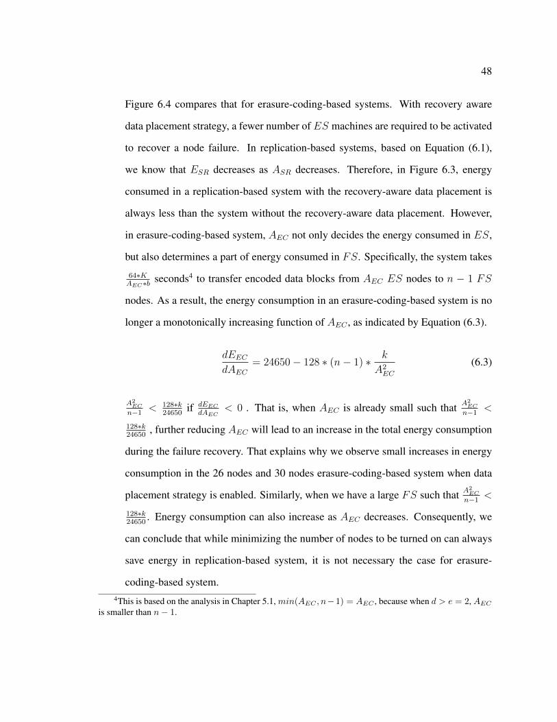
to recover a node failure. In replication-based systems, based on Equation (6.1),

we know that ESR decreases as ASR decreases. Therefore, in Figure 6.3, energy

consumed in a replication-based system with the recovery-aware data placement is

always less than the system without the recovery-aware data placement. However,

in erasure-coding-based system, AEC not only decides the energy consumed in ES,

but also determines a part of energy consumed in FS. Specifically, the system takes

64∗KAEC∗b seconds4 to transfer encoded data blocks from AEC ES nodes to n − 1 FS

nodes. As a result, the energy consumption in an erasure-coding-based system is no

longer a monotonically increasing function of AEC , as indicated by Equation (6.3).

dEEC

dAEC

= 24650− 128 ∗ (n− 1) ∗ k

A2EC

(6.3)

A2EC

n−1< 128∗k

24650if dEEC

dAEC< 0 . That is, when AEC is already small such that A2

EC

n−1<

128∗k24650

, further reducing AEC will lead to an increase in the total energy consumption

during the failure recovery. That explains why we observe small increases in energy

consumption in the 26 nodes and 30 nodes erasure-coding-based system when data

placement strategy is enabled. Similarly, when we have a large FS such that A2EC

n−1<

128∗k24650

. Energy consumption can also increase as AEC decreases. Consequently, we

can conclude that while minimizing the number of nodes to be turned on can always

save energy in replication-based system, it is not necessary the case for erasure-

coding-based system.4This is based on the analysis in Chapter 5.1, min(AEC , n−1) = AEC , because when d > e = 2, AEC

is smaller than n− 1.

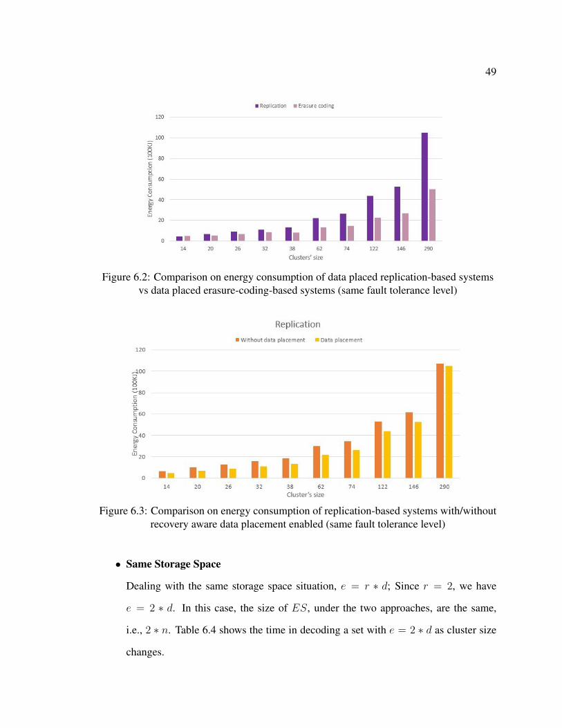
49

Figure 6.2: Comparison on energy consumption of data placed replication-based systemsvs data placed erasure-coding-based systems (same fault tolerance level)

Figure 6.3: Comparison on energy consumption of replication-based systems with/withoutrecovery aware data placement enabled (same fault tolerance level)

• Same Storage Space

Dealing with the same storage space situation, e = r ∗ d; Since r = 2, we have

e = 2 ∗ d. In this case, the size of ES, under the two approaches, are the same,

i.e., 2 ∗ n. Table 6.4 shows the time in decoding a set with e = 2 ∗ d as cluster size

changes.

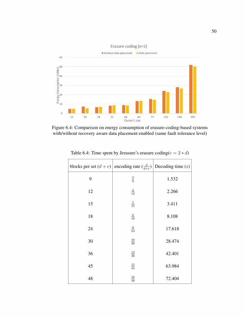
50

Figure 6.4: Comparison on energy consumption of erasure-coding-based systemswith/without recovery aware data placement enabled (same fault tolerance level)

Table 6.4: Time spent by Jerasure’s erasure coding(e = 2 ∗ d)

blocks per set (d+ e) encoding rate ( dd+e

) Decoding time (s)

9 39

1.532

12 412

2.266

15 515

3.411

18 618

8.108

24 824

17.618

30 1030

28.474

36 1236

42.401

45 1545

63.984

48 1648

72.404

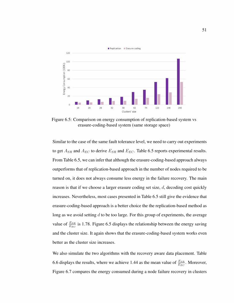
51

Figure 6.5: Comparison on energy consumption of replication-based system vserasure-coding-based system (same storage space)

Similar to the case of the same fault tolerance level, we need to carry out experiments

to get ASR and AEC to derive ESR and EEC . Table 6.5 reports experimental results.

From Table 6.5, we can infer that although the erasure-coding-based approach always

outperforms that of replication-based approach in the number of nodes required to be

turned on, it does not always consume less energy in the failure recovery. The main

reason is that if we choose a larger erasure coding set size, d, decoding cost quickly

increases. Nevertheless, most cases presented in Table 6.5 still give the evidence that

erasure-coding-based approach is a better choice the the replication-based method as

long as we avoid setting d to be too large. For this group of experiments, the average

value of ESR

EECis 1.78. Figure 6.5 displays the relationship between the energy saving

and the cluster size. It again shows that the erasure-coding-based system works even

better as the cluster size increases.

We also simulate the two algorithms with the recovery aware data placement. Table

6.6 displays the results, where we achieve 1.44 as the mean value of ESR

EEC. Moreover,

Figure 6.7 compares the energy consumed during a node failure recovery in clusters

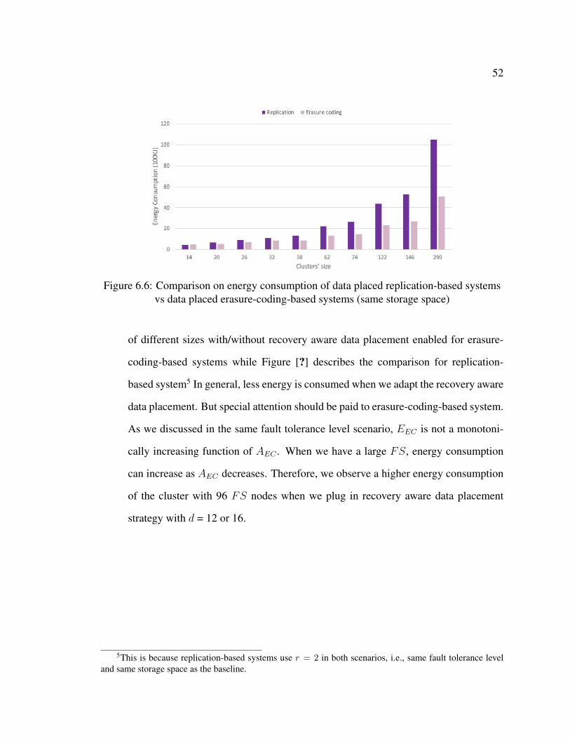
52

Figure 6.6: Comparison on energy consumption of data placed replication-based systemsvs data placed erasure-coding-based systems (same storage space)

of different sizes with/without recovery aware data placement enabled for erasure-

coding-based systems while Figure [?] describes the comparison for replication-

based system5 In general, less energy is consumed when we adapt the recovery aware

data placement. But special attention should be paid to erasure-coding-based system.

As we discussed in the same fault tolerance level scenario, EEC is not a monotoni-

cally increasing function of AEC . When we have a large FS, energy consumption

can increase as AEC decreases. Therefore, we observe a higher energy consumption

of the cluster with 96 FS nodes when we plug in recovery aware data placement

strategy with d = 12 or 16.

5This is because replication-based systems use r = 2 in both scenarios, i.e., same fault tolerance leveland same storage space as the baseline.

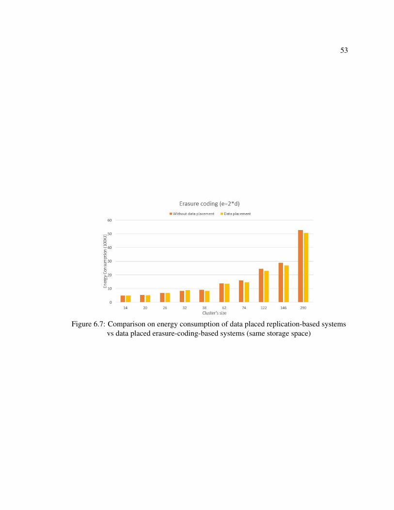
53

Figure 6.7: Comparison on energy consumption of data placed replication-based systemsvs data placed erasure-coding-based systems (same storage space)

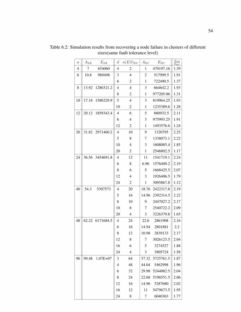
54

Table 6.2: Simulation results from recovering a node failure in clusters of differentsizes(same fault tolerance level)

n ASR ESR d n(ES)EC AEC EECESR

EEC

4 7 654060 4 2 1 470197.16 1.39

6 10.8 989498 3 4 2 517999.5 1.91

6 2 1 722490.5 1.37

8 13.92 1280321.2 4 4 3 664642.2 1.93

8 2 1 977205.06 1.31

10 17.18 1580329.9 5 4 3 819964.25 1.93

10 2 1 1235389.6 1.28

12 20.12 1859343.4 4 6 5 880932.5 2.11

6 4 3 975993.25 1.91

12 2 1 1493576.6 1.24

20 31.82 2971460.2 4 10 9 1320795 2.25

5 8 7 1338073.1 2.22

10 4 3 1608085.4 1.85

20 2 1 2546802.5 1.17

24 36.56 3454691.8 4 12 11 1541719.1 2.24

6 8 6.96 1576409.2 2.19

8 6 5 1668425.5 2.07

12 4 3 1926406.5 1.79

24 2 1 3095867.8 1.12

40 54.3 5307573 4 20 18.76 2422317.8 2.19

5 16 14.96 2392314.5 2.22

8 10 9 2447027.2 2.17

10 8 7 2540722.2 2.09

20 4 3 3226379.8 1.65

48 62.22 6171684.5 4 24 22.6 2861908 2.16

6 16 14.94 2801881 2.2

8 12 10.98 2839133 2.17

12 8 7 3026123.5 2.04

16 6 5 3274527 1.88

24 4 3 3905724 1.58

96 99.48 1.07E+07 3 64 57.32 5725761.5 1.87

4 48 44.04 5462998 1.96

6 32 29.98 5244082.5 2.04

8 24 22.68 5196551.5 2.06

12 16 14.96 5287680 2.02

16 12 11 5479673.5 1.95

24 8 7 6040363 1.77

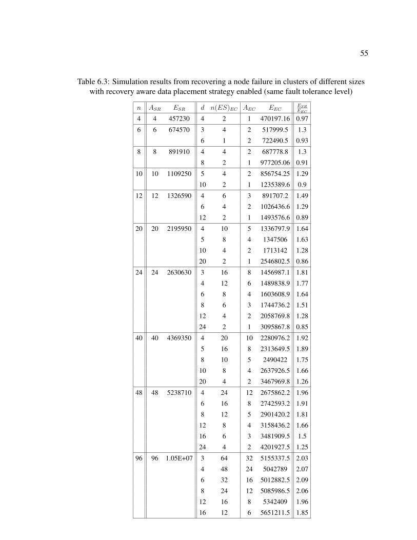
55

Table 6.3: Simulation results from recovering a node failure in clusters of different sizeswith recovery aware data placement strategy enabled (same fault tolerance level)

n ASR ESR d n(ES)EC AEC EECESR

EEC

4 4 457230 4 2 1 470197.16 0.97

6 6 674570 3 4 2 517999.5 1.3

6 1 2 722490.5 0.93

8 8 891910 4 4 2 687778.8 1.3

8 2 1 977205.06 0.91

10 10 1109250 5 4 2 856754.25 1.29

10 2 1 1235389.6 0.9

12 12 1326590 4 6 3 891707.2 1.49

6 4 2 1026436.6 1.29

12 2 1 1493576.6 0.89

20 20 2195950 4 10 5 1336797.9 1.64

5 8 4 1347506 1.63

10 4 2 1713142 1.28

20 2 1 2546802.5 0.86

24 24 2630630 3 16 8 1456987.1 1.81

4 12 6 1489838.9 1.77

6 8 4 1603608.9 1.64

8 6 3 1744736.2 1.51

12 4 2 2058769.8 1.28

24 2 1 3095867.8 0.85

40 40 4369350 4 20 10 2280976.2 1.92

5 16 8 2313649.5 1.89

8 10 5 2490422 1.75

10 8 4 2637926.5 1.66

20 4 2 3467969.8 1.26

48 48 5238710 4 24 12 2675862.2 1.96

6 16 8 2742593.2 1.91

8 12 5 2901420.2 1.81

12 8 4 3158436.2 1.66

16 6 3 3481909.5 1.5

24 4 2 4201927.5 1.25

96 96 1.05E+07 3 64 32 5155337.5 2.03

4 48 24 5042789 2.07

6 32 16 5012882.5 2.09

8 24 12 5085986.5 2.06

12 16 8 5342409 1.96

16 12 6 5651211.5 1.85

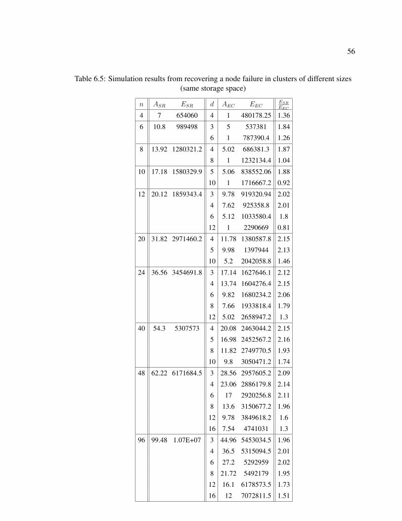
56

Table 6.5: Simulation results from recovering a node failure in clusters of different sizes(same storage space)

n ASR ESR d AEC EECESR

EEC

4 7 654060 4 1 480178.25 1.36

6 10.8 989498 3 5 537381 1.84

6 1 787390.4 1.26

8 13.92 1280321.2 4 5.02 686381.3 1.87

8 1 1232134.4 1.04

10 17.18 1580329.9 5 5.06 838552.06 1.88

10 1 1716667.2 0.92

12 20.12 1859343.4 3 9.78 919320.94 2.02

4 7.62 925358.8 2.01

6 5.12 1033580.4 1.8

12 1 2290669 0.81

20 31.82 2971460.2 4 11.78 1380587.8 2.15

5 9.98 1397944 2.13

10 5.2 2042058.8 1.46

24 36.56 3454691.8 3 17.14 1627646.1 2.12

4 13.74 1604276.4 2.15

6 9.82 1680234.2 2.06

8 7.66 1933818.4 1.79

12 5.02 2658947.2 1.3

40 54.3 5307573 4 20.08 2463044.2 2.15

5 16.98 2452567.2 2.16

8 11.82 2749770.5 1.93

10 9.8 3050471.2 1.74

48 62.22 6171684.5 3 28.56 2957605.2 2.09

4 23.06 2886179.8 2.14

6 17 2920256.8 2.11

8 13.6 3150677.2 1.96

12 9.78 3849618.2 1.6

16 7.54 4741031 1.3

96 99.48 1.07E+07 3 44.96 5453034.5 1.96

4 36.5 5315094.5 2.01

6 27.2 5292959 2.02

8 21.72 5492179 1.95

12 16.1 6178573.5 1.73

16 12 7072811.5 1.51

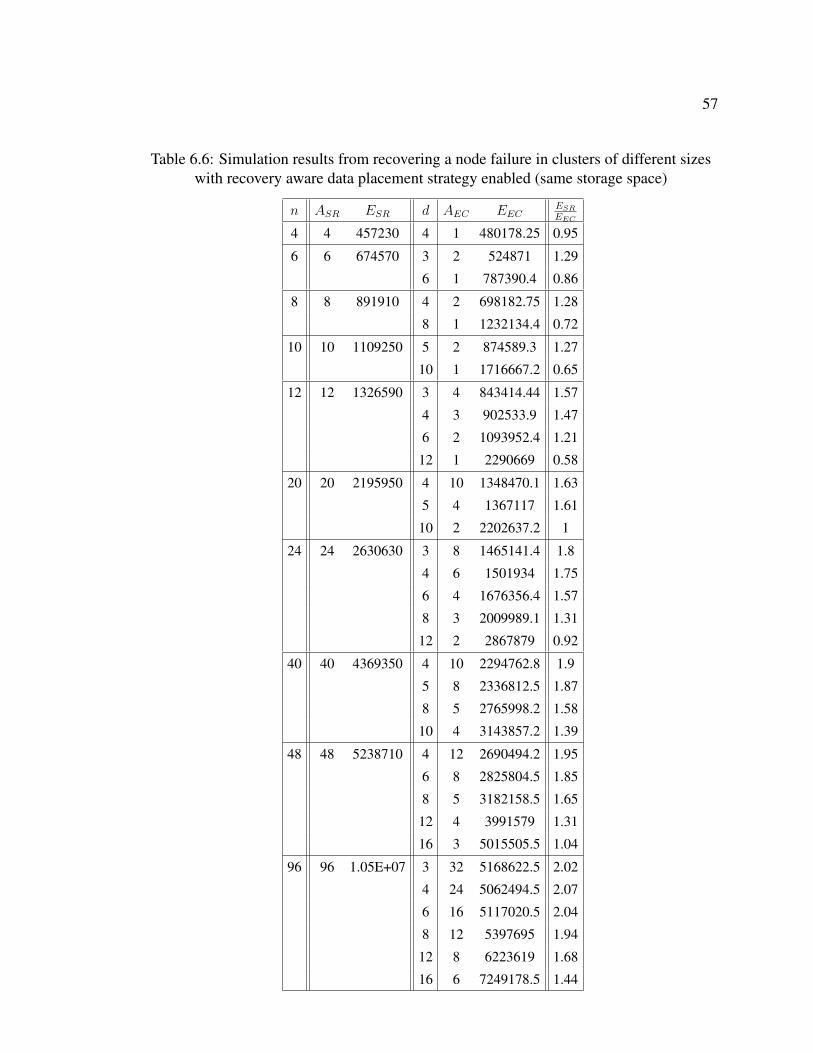
57

Table 6.6: Simulation results from recovering a node failure in clusters of different sizeswith recovery aware data placement strategy enabled (same storage space)

n ASR ESR d AEC EECESR

EEC

4 4 457230 4 1 480178.25 0.95

6 6 674570 3 2 524871 1.29

6 1 787390.4 0.86

8 8 891910 4 2 698182.75 1.28

8 1 1232134.4 0.72

10 10 1109250 5 2 874589.3 1.27

10 1 1716667.2 0.65

12 12 1326590 3 4 843414.44 1.57

4 3 902533.9 1.47

6 2 1093952.4 1.21

12 1 2290669 0.58

20 20 2195950 4 10 1348470.1 1.63

5 4 1367117 1.61

10 2 2202637.2 1

24 24 2630630 3 8 1465141.4 1.8

4 6 1501934 1.75

6 4 1676356.4 1.57

8 3 2009989.1 1.31

12 2 2867879 0.92

40 40 4369350 4 10 2294762.8 1.9

5 8 2336812.5 1.87

8 5 2765998.2 1.58

10 4 3143857.2 1.39

48 48 5238710 4 12 2690494.2 1.95

6 8 2825804.5 1.85

8 5 3182158.5 1.65

12 4 3991579 1.31

16 3 5015505.5 1.04

96 96 1.05E+07 3 32 5168622.5 2.02

4 24 5062494.5 2.07

6 16 5117020.5 2.04

8 12 5397695 1.94

12 8 6223619 1.68

16 6 7249178.5 1.44

58

Chapter 7

Conclusion

In this thesis, we investigate an energy efficient failure recovery problem in a storage cluster

which adopts both a power saving technique and a redundancy mechanism and an erasure

coding technique. Specifically, with the purpose of energy saving, only one copy of the

original data blocks are stored in Fundamental Set (FS) and are kept online. However,

data could be corrupted or node could fail in FS. Redundant information in Extended

Set (ES) is used to restore the lost data. To study energy-efficient failure recovery, we

consider two different data redundancy mechanisms, i.e., replication and erasure coding.

We first develop greedy recovery algorithms for the two systems and then a recovery aware

data placement policy to further improve the failure recovery efficiency. For this study,

we build energy models and use data collected from our testbed cluster to analyze and

estimate the energy cost in recovering a node failure. Simulation results show that, in

general, erasure-coding-based system saves about 40% of the energy in a failure recovery

when compared with replication-based system. Besides, we also observe that the recovery

aware data placement strategy always benefits replication-based systems and also gains

energy saving for medium-sized erasure-coding-based systems.

59

Chapter 8

Future Work

We have simulated and analyzed the energy consumption under different scenarios using

data profiled from our testbed cluster. In the future, we plan to validate our simulation

results by deploying the failure recovery algorithms in a publicly accessible medium size

cluster, i.e., Green Server Farm at University of Illinois at Urbana-Champaign. In this

thesis, we have considered a single node failure. We will study the energy efficient multi-

node failure recovery problem in the future.

60

Bibliography

[1] Marcos K. Aguilera and Ramaprabhu Janakiraman. Using erasure codes efficiently

for storage in a distributed system. In In Proc. of DSN05, pages 336–345. IEEE

Computer Society, 2005.

[2] Luiz Andre Barroso and Urs Holzle. The case for energy-proportional computing.

Computer, 40(12):33–37, December 2007.

[3] Abdlmonem H. Beitelmal and Chandrakant D. Patel. Thermo-fluids provisioning of a

high performance high density data center. Distrib. Parallel Databases, 21(2-3):227–

238, June 2007.

[4] Emerson Network Power. Energy Logic: Reducing Data Center Energy Consumption

by Creating Savings that Cascade Across Systems, November 2007.

[5] Bin Fan, Wittawat Tantisiriroj, Lin Xiao, and Garth Gibson. Diskreduce: Raid for

data-intensive scalable computing. In Proceedings of the 4th Annual Workshop on

Petascale Data Storage, PDSW ’09, pages 6–10, New York, NY, USA, 2009. ACM.

[6] Xiaobo Fan, Wolf dietrich Weber, and Luiz Andr Barroso. Power provisioning for a

warehouse-sized computer. In In Proceedings of ISCA, 2007.

[7] Anshul Gandhi, Mor Harchol-Balter, Rajarshi Das, and Charles Lefurgy. Optimal

power allocation in server farms. In Proceedings of the eleventh international joint

61

conference on Measurement and modeling of computer systems, SIGMETRICS ’09,

pages 157–168, New York, NY, USA, 2009. ACM.

[8] Cristian A. Gonzalez. Understand hadoop at first look, 2010.

[9] Sriram Govindan, Jeonghwan Choi, Bhuvan Urgaonkar, Anand Sivasubramaniam,

and Andrea Baldini. Statistical profiling-based techniques for effective power pro-

visioning in data centers. In Proceedings of the 4th ACM European conference on

Computer systems, EuroSys ’09, pages 317–330, New York, NY, USA, 2009. ACM.

[10] Apache Hadoop. Apache hadoop, 2013.

[11] Apache Hadoop. Hadoop 1.0.4 documentation, 2013.

[12] Apache Hadoop. What is apache hadoop?, 2013.

[13] Andrew Krioukov, Prashanth Mohan, Sara Alspaugh, Laura Keys, David Culler, and

Randy H. Katz. Napsac: design and implementation of a power-proportional web

cluster. In Proceedings of the first ACM SIGCOMM workshop on Green networking,

Green Networking ’10, pages 15–22, New York, NY, USA, 2010. ACM.

[14] John Kubiatowicz, David Bindel, Yan Chen, Steven Czerwinski, Patrick Eaton,

Dennis Geels, Ramakrishan Gummadi, Sean Rhea, Hakim Weatherspoon, Westley

Weimer, Chris Wells, and Ben Zhao. Oceanstore: an architecture for global-scale

persistent storage. SIGPLAN Not., 35(11):190–201, November 2000.

[15] Willis Lang and Jignesh M. Patel. Energy management for mapreduce clusters.

PVLDB, 3(1):129–139, 2010.

[16] Jacob Leverich and Christos Kozyrakis. On the energy (in)efficiency of hadoop clus-

ters. SIGOPS Oper. Syst. Rev., 44:61–65, March 2010.

62

[17] Shu Lin and D.J. Costello. Error control coding: fundamentals and applications.

Prentice-Hall computer applications in electrical engineering series. Prentice-Hall,

1983.

[18] Jianqiang Luo, Mochan Shrestha, and Lihao Xu. Hyfs: A highly available distributed

file system.

[19] John Markoff. Data centers’s power use less than was expected, 2011.

[20] David Meisner, Brian T. Gold, and Thomas F. Wenisch. Powernap: eliminating server

idle power. In ASPLOS’09, pages 205–216, 2009.

[21] Steven Pelley, David Meisner, Pooya Zandevakili, Thomas F. Wenisch, and Jack Un-

derwood. Power routing: dynamic power provisioning in the data center. SIGPLAN

Not., 45(3):231–242, March 2010.

[22] Ramya Raghavendra, Parthasarathy Ranganathan, Vanish Talwar, Zhikui Wang, and

Xiaoyun Zhu. No ”power” struggles: coordinated multi-level power management for

the data center. In Proceedings of the 13th international conference on Architectural

support for programming languages and operating systems, ASPLOS XIII, pages 48–

59, New York, NY, USA, 2008. ACM.

[23] Catherine D. Schuman and James S. Plank. A performance comparison of open-

source erasure coding libraries for storage applications. Technical report, 2008.

[24] Andrew S. Tanenbaum and M. Van Steen. Distributed Systems: Principles and

Paradigms. Prentice Hall, 2001.

[25] U.S. Department of Energy. Quick Start Guide to Increase Data Center Energy Effi-

ciency, 2010.

63

[26] Hakim Weatherspoon and John Kubiatowicz. Erasure coding vs. replication: A quan-

titative comparison. In Revised Papers from the First International Workshop on

Peer-to-Peer Systems, IPTPS ’01, pages 328–338, London, UK, UK, 2002. Springer-

Verlag.

[27] Tom White. Hadoop: The Definitive Guide. O’Reilly Media, original edition, June

2009.