Energy efficiency gains from trade in

intermediate inputs: firm-level evidence from

Indonesia

Michele Imbruno and Tobias Ketterer

June 2016

Centre for Climate Change Economics and Policy

Working Paper No. 274

Grantham Research Institute on Climate Change and

the Environment

Working Paper No. 244

The Centre for Climate Change Economics and Policy (CCCEP) was established by the University of Leeds and the London School of Economics and Political Science in 2008 to advance public and private action on climate change through innovative, rigorous research. The Centre is funded by the UK Economic and Social Research Council. Its second phase started in 2013 and there are five integrated research themes:

1. Understanding green growth and climate-compatible development 2. Advancing climate finance and investment 3. Evaluating the performance of climate policies 4. Managing climate risks and uncertainties and strengthening climate services 5. Enabling rapid transitions in mitigation and adaptation

More information about the Centre for Climate Change Economics and Policy can be found at: http://www.cccep.ac.uk. The Grantham Research Institute on Climate Change and the Environment was established by the London School of Economics and Political Science in 2008 to bring together international expertise on economics, finance, geography, the environment, international development and political economy to create a world-leading centre for policy-relevant research and training. The Institute is funded by the Grantham Foundation for the Protection of the Environment and the Global Green Growth Institute. It has nine research programmes:

1. Adaptation and development 2. Carbon trading and finance 3. Ecosystems, resources and the natural environment 4. Energy, technology and trade 5. Future generations and social justice 6. Growth and the economy 7. International environmental negotiations 8. Modelling and decision making 9. Private sector adaptation, risk and insurance

More information about the Grantham Research Institute on Climate Change and the Environment can be found at: http://www.lse.ac.uk/grantham. This working paper is intended to stimulate discussion within the research community and among users of research, and its content may have been submitted for publication in academic journals. It has been reviewed by at least one internal referee before publication. The views expressed in this paper represent those of the author(s) and do not necessarily represent those of the host institutions or funders.

1

Energy efficiency gains from trade in intermediate inputs:

Firm-level evidence from Indonesia

Michele Imbruno a Tobias D. Ketterer

b

Abstract

This paper investigates whether importing intermediate goods improves firm-level

environmental performance in a developing country, using data from the Indonesian

manufacturing sector. We build a simple theoretical model showing that trade integration of

input markets entails energy efficiency improvements within importers relative to non-

importers. To empirically isolate the impact of firm participation in foreign intermediate

input markets we use ‘nearest neighbour’ propensity score matching and difference-in-

difference techniques. Covering the period 1991-2005, we find evidence that becoming an

importer of foreign intermediates boosts energy efficiency, implying beneficial effects for the

environment.

JEL: F12, F14, F18, Q56

Keywords: Trade, Intermediate Inputs, Energy Efficiency, Environment and Indonesia

Acknowledgements. The authors would like to thank Sotiris Blanas, Antoine Dechezlepretre, Ana M.

Fernandes, Beata Javorcik, Richard Kneller, Alessia Lo Turco, Daniela Maggioni, and all participants at the

ETSG 2015 Conference in Paris and CSAE 2016 Conference at Oxford University for their helpful comments

and suggestions. Michele Imbruno gratefully acknowledges financial support from the CrisisLab project funded

by the Italian government. Tobias Ketterer gratefully acknowledges financial support from the ESRC Centre for

Climate Change Economics and Policy. This paper reflects the views of the authors only and should not be

attributed to the European Commission.

a

IMT Institute for Advanced Studies, Lucca (Italy), and GEP, Nottingham (UK). E-mail address:

michele.imbruno@imtlucca.it. b Directorate-General for Economic and Financial Affairs, European Commission, Brussels. E-mail address:

tobias.ketterer@ec.europa.eu.

2

1. Introduction

Globalisation and the formation of global supply chains have led to a substantial increase not

only in the trade in final goods, but also in intermediate goods. Previous research has shown

that access to cheaper imported inputs results in important productivity gains based on firms’

access to a larger number of input varieties, a better input quality, and technology transfers

(Ethier, 1982; Markusen, 1989; Grossman and Helpman, 1991).1 Access to foreign input

markets and with it enhanced learning, quality and variety effects, may lower the costs of

innovation and generate sizable dynamic gains from trade with important consequences for

firm-level product scope and firm efficiency. Previous empirical work shows that trade

liberalisation in intermediate input markets represents a significant source of firm level

productivity gains in Brazil (Schor, 2004), Indonesia (Amiti and Konings, 2008) and India

(Goldberg et al., 2010; Khandelwal and Topalova, 2011); with productivity gains from

intermediate input tariff reductions likely to exceed those stemming from tariff cuts for final

goods.

At the same time, increasing international trade flows have sparked a vibrant debate

featuring a growing concern over the impact of globalisation on the environment. Enunciated

by the pollution haven hypothesis, the possibility of major trade reforms resulting in a shift of

pollution-intensive activities to territories with weaker environmental standards raised fears

of a global race to the bottom and increasing global pollution. Theoretical evidence on the

link between trade and the environment, however, tends to be ambiguous and does not

provide a clear verdict. Advanced by the seminal contributions of Pethig (1976) and McGuire

(1982) the pollution haven hypothesis has also been put into perspective in studies

considering that environmental policy may respond to changes in trade patterns (Copeland

and Taylor, 1994, 1995), or when allowing for differences in income and factor abundance to

jointly determine the patterns of trade (Antweiler et al., 2001).2

Empirical studies on the effect of trade and trade policy reform on environmental

performance at the detailed firm level are scarce and mainly focus on firms’ decision to

1 A related literature highlights aggregate productivity gains stemming from new exporting opportunities and

increasing competition following trade liberalisation (Melitz, 2003; Melitz and Ottaviano, 2008), and firm-level

productivity gains associated with intra-firm reallocation of resources (Bernard, Redding and Schott, 2006). 2 Further theoretical contributions include, amongst others, Barret (1994), Markusen et al. (1995), Copeland and

Taylor (1997), who additionally consider governments’ strategic incentives, the location-specific character of

pollution, and differences in factor endowments, respectively.

3

export in an industrialised country context.3 Galdeano-Gómez (2010), for instance, considers

the relationship between export orientation and environmental performance in the Spanish

food industry, and provides evidence for a positive correlation. Girma et al. (2008)

investigate environmental firm performance in a Melitz-type (2003) heterogeneous firms

framework and provide evidence for exporting status being positively associated with the

propensity to adopt newer and, hence, more advanced and environmentally-sound

technologies, given exporters’ larger ability to amortise fixed investment costs, relative to

non-exporters. They provide empirical support for their theoretical predictions by using UK

survey data showing that exporters tend to consider their innovations to be more energy-

efficient and environmentally-sound. Batrakova and Davies (2012) extend the literature by

looking at the impact of exporting status on actual energy use as a measure for environmental

performance. Using a partial equilibrium framework and Irish firm-level data, they show that

while exporting leads to energy efficiency losses for firms with low energy intensity because

of predominant scale effects, high energy intensity firms are likely to become more energy

efficient as they are pushed to invest in energy-saving technologies. 4

Against the backdrop of a relatively limited firm-level literature on the international

trade-environment nexus, this paper contributes to the existing literature by examining the

impact of foreign intermediate inputs (rather than exports) on firms’ productivity and

environmental performance, in the context of a developing country. We begin by developing

a simple theoretical framework, mainly based on Krugman (1980) and Ethier (1982), with

two vertically-related sectors, where symmetric firms supply their varieties under

monopolistic competition and in an autarkic regime. Firms in the downstream sector produce

final good varieties, by mainly using energy and intermediate inputs, which are in turn

manufactured by firms in the upstream sector. Next, we study the impact of trade integration

of intermediate input markets across identical countries on firm-level energy intensity, in

addition to productivity. We assume that only a given fraction of final good producers are

able to import, whereas the other firms are not able to do so. We show that firms that enter

intermediate input markets increase, on average, their performance, and reduce their energy

intensity, compared with non-importing firms. In other words, through importing, firms have

access to a larger range of differentiated intermediate inputs, which entails not only a more

efficient usage of intermediates itself (productivity gains à la Ethier, 1982), but also a more

3 More aggregate empirical work tends to provide evidence for trade encouraging the development of more

environmentally sound production processes (Levinson, 2009; Dean and Lovely, 2008; Antweiler et al., 2001). 4 Kaiser and Schulze (2003) examine the effect of export decisions on environmental expenses and find a

positive correlation.

4

efficient usage of energy, implying beneficial effects for the environment (environmental

gains from input varieties).5

We test the theoretical predictions by using firm-level data on manufacturing firms in

Indonesia covering the time period 1991 to 2005. Using propensity-score matching and

difference-in-difference techniques, the empirical findings support the results of our model by

providing evidence for import-status being positively correlated with an increase in firm

efficiency and a decline in firm-level energy intensities.6 Accounting for export status and

FDI status corroborates our findings for firm-level efficiency and environmental

performance. Our results may hence carry important implication as they tend to suggest that

trade liberalisation and access to foreign intermediate input markets may generate important

economic but also environmental benefits for producers in emerging markets.

Our work can be considered one of the first attempts aiming to explore how importing

intermediate inputs may affect firm-level energy efficiency. To our knowledge, a similar

issue has only been addressed by Martin (2011). Using firm-level panel data, she examines

changes in energy efficiency following trade, FDI and licensing reforms in India. Martin

(2011) findings show that trade liberalisation in intermediate input markets entails, on

average, within-industry energy efficiency gains based on within firm improvements only.7

Our analysis, however, contrasts with Martin's (2011), first, by providing an analytical

framework which aims to show that firms starting to import intermediate inputs gain in

energy efficiency compared with firms that remain non-importers. Second, we empirically

quantify these energy efficiency gains from importing intermediate inputs, by directly

comparing the change in energy intensity between import-starters and firms that remain non-

importers with similar initial characteristics, to control for potential self-selection into

importing activities.

The reminder of the paper is structured as follows. Section 2 outlines a very simple

theoretical framework designed to focus and guide our empirical investigation. Section 3

introduces our empirical identification strategy, and provides a description of the data and the

most salient sample characteristics. The empirical findings for the correlation between

5 Note that in our theoretical set-up, we only allow for importing gains stemming from a larger set of input

varieties. We, however, acknowledge that in reality gains from input importing may also arise through other

channels, such as quality and/or learning effects (cf. Markusen, 1989; Grossman and Helpman, 1990). 6 Since there is no pollution data available at the firm level, we use energy intensities, i.e. energy use divided by

total output. This approach is similar to the strategy chosen by Eskeland and Harrison (2003) and Cole et al.

(2008). 7 She also documents that, while FDI liberalisation and delicensing leads to a reallocation of market shares from

the least to the most energy-efficient firms, a reduction in tariffs on intermediate inputs results in a reallocation

towards the least efficient firms instead.

5

intermediate input importing status and environmental firm performance are presented and

discussed in section 4. Section 5 concludes.

2. Theoretical framework

In this section we present a very simple theoretical model, mainly based on both

Krugman (1980) and Ethier (1982), to guide our empirical investigation. The purpose of this

is to formulate some predictions on how importing intermediate inputs may affect energy

efficiency at the firm-level. We first present a closed economy model with two sectors

vertically related to each other, where symmetric firms supply their goods in monopolistic

competitive markets. In particular, we assume that the downstream sector produces its final

good varieties, by mainly using energy and intermediate inputs, which are, in turn, produced

by the upstream sector. The upstream sector mainly uses labour. Material inputs are assumed

to be horizontally differentiated, which is a common feature in the literature when

investigating the effects of international trade on total factor productivity (cf. Ethier, 1982;

Romer, 1990; Grossman and Helpman, 1991).

Next, we study how trade openness in the intermediate input markets may influence

firm-level energy intensity, in addition to firm performance. We thereby assume that only a

given fraction of final good producers are able to access foreign intermediate input market

(i.e. importers), whereas the other firms are not able to do so (i.e. non-importers).8

2.1 Closed Economy

Final good sector. Consider a setting in which consumers supply labour L to firms at

a wage rate w, and, at the same time, demand all available final differentiated varieties (y)

produced by domestic firms. In particular, consumers are assumed to show CES preferences,

so that the demand for each variety y is given by 1

yyyy PRypyq , where yp

represents the price of a single variety y, and

1

1

0

1N

yy dyypP is the aggregate price

index of all available final varieties N. yR denotes aggregate revenue in the final goods

8 For simplicity, we abstract from the underlying reasons. In our case, where firms are assumed to be symmetric

in both sectors, it could be because of a random allocation of import licenses. But, in a more sophisticated case,

where firms can be assumed to be heterogeneous in initial productivity, it could be because of a self-selection

mechanisms: i.e. only the more productive firms are able to import (Gibson and Graciano, 2011, Imbruno,

2014).

6

sector, which is equal to aggregate consumer income (wL). The wage rate w represents our

numeraire (i.e. w=1). 1 denotes the elasticity of substitution between final good varieties.

We model final good firms' output production, yq , by means of the following Cobb-Douglas

technology function:

1

meyy XXq , with 1

0

1

M

mm dmmxX

where y denotes the firm-level Hicksian productivity, eX stands for energy consumption e,

and mX denotes CES consumption in intermediate inputs m. and 1 represent the

factor shares of production. Notice that firm-level aggregate consumption in intermediates is

a function of the total number of all symmetric intermediate input varieties ( M ), the quantity

consumed of each input variety ( mx ), and the elasticity of substitution between them ( 1

), as in Ethier (1982). Thus, firm-level demands in energy and intermediate inputs can

respectively be written as:

11

1 e

m

y

y

eP

PqX

m

e

y

y

mP

PqX

1

Firm-level demand of a single intermediate input variety m is given by

mmmm XPpx

, where mpm represents the price of intermediate variety m,

1

1

0

1M

mm dmmpP the aggregate intermediate input price, and eP denotes the

aggregate energy price. It is worth pointing out that, while mP is considered to be

endogenous, eP is modelled to be exogenous as energy is assumed to be in-elastically

supplied within a country (similarly to labour).9

Under profit maximisation, each firm will charge a price equal to

ymey PPp

1

1

1

,where )1(

1

. Domestic firms' profit may, hence,

be expressed as y

y

mey q

PP

1

1

, which alternatively can also be written as N

Ry

y

.

9 Larch and Wanner (2015) make a similar assumption. The authors argue that a constant energy price is quite

plausible, by considering the oil market characteristics and the important role played by OPEC, which may have

incentives to adjust the oil supply to keep oil prices stable.

7

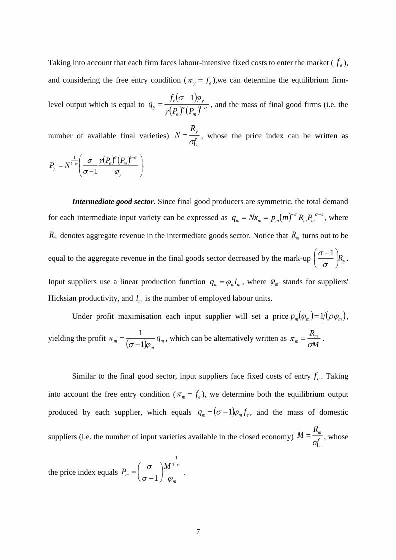
Taking into account that each firm faces labour-intensive fixed costs to enter the market ( ef ),

and considering the free entry condition ( ey f ),we can determine the equilibrium firm-

level output which is equal to

1

1

me

ye

yPP

fq , and the mass of final good firms (i.e. the

number of available final varieties) e

y

f

RN

, whose the price index can be written as

y

mey

PPNP

1

1

1

1.

Intermediate good sector. Since final good producers are symmetric, the total demand

for each intermediate input variety can be expressed as 1

mmmmm PRmpNxq , where

mR denotes aggregate revenue in the intermediate goods sector. Notice that mR turns out to be

equal to the aggregate revenue in the final goods sector decreased by the mark-up yR

1.

Input suppliers use a linear production function mmm lq , where m stands for suppliers'

Hicksian productivity, and ml is the number of employed labour units.

Under profit maximisation each input supplier will set a price mmmp 1 ,

yielding the profit m

m

m q

1

1

, which can be alternatively written as

M

Rmm

.

Similar to the final good sector, input suppliers face fixed costs of entry ef . Taking

into account the free entry condition ( em f ), we determine both the equilibrium output

produced by each supplier, which equals emm fq 1 , and the mass of domestic

suppliers (i.e. the number of input varieties available in the closed economy) e

m

f

RM

, whose

the price index equals m

m

MP

1

1

1.

8

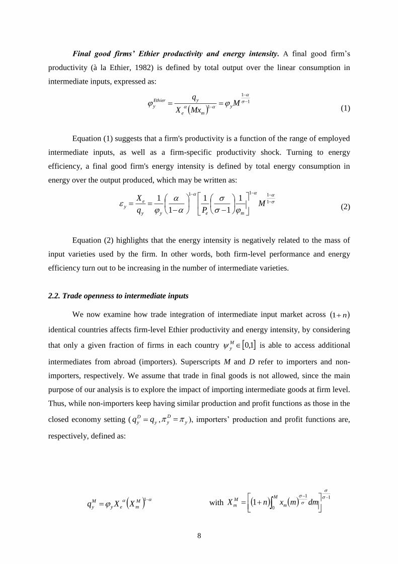
Final good firms’ Ethier productivity and energy intensity. A final good firm’s

productivity (à la Ethier, 1982) is defined by total output over the linear consumption in

intermediate inputs, expressed as:

1

1

1

M

MxX

qy

me

yEthier

y

(1)

Equation (1) suggests that a firm's productivity is a function of the range of employed

intermediate inputs, as well as a firm-specific productivity shock. Turning to energy

efficiency, a final good firm's energy intensity is defined by total energy consumption in

energy over the output produced, which may be written as:

1

1111

1

1

1

1M

Pq

X

meyy

ey

(2)

Equation (2) highlights that the energy intensity is negatively related to the mass of

input varieties used by the firm. In other words, both firm-level performance and energy

efficiency turn out to be increasing in the number of intermediate varieties.

2.2. Trade openness to intermediate inputs

We now examine how trade integration of intermediate input market across n1

identical countries affects firm-level Ethier productivity and energy intensity, by considering

that only a given fraction of firms in each country 1,0M

y is able to access additional

intermediates from abroad (importers). Superscripts M and D refer to importers and non-

importers, respectively. We assume that trade in final goods is not allowed, since the main

purpose of our analysis is to explore the impact of importing intermediate goods at firm level.

Thus, while non-importers keep having similar production and profit functions as those in the

closed economy setting ( y

D

y qq , y

D

y ), importers’ production and profit functions are,

respectively, defined as:

1M

mey

M

y XXq with 1

0

1

1

M

m

M

m dmmxnX

9

M

y

y

M

meM

y qPP

1

1

with

1

1

0

11

M

m

M

m dmmpnP

,

It is worth noting that both importers' production and profit functions can be

expressed in relative terms to those of non-importers – i.e. D

y

M

y qnq

1

11 , and

D

y

M

y n

1

1 .

Consequently, the average profit within the final good sector is given by

D

y

y

D

meM

y

M

yy qPP

n

111~

1

1

, which alternatively can also be written as

N

Ry

y

~ . As in Melitz (2003), we also assume that firms will only enter the market if the

expected profit is higher than the fixed cost of entry ef . Thus, using the free entry condition (

ey f~ ), we can determine both non-importer and importer output levels as:

yM

y

M

y

D

me

yeD

y qnPP

fq

1111

1

yD

me

ye

M

y

M

y

D

y

M

y qPP

f

n

nqnq

11

111

1

1

11

11

The resulting number of all domestic final good firms equals e

y

f

RN

, and the related price

index amounts to

y

MM

D

mey

nPPNP

1

111

1

111

.

Taking into account that firm-level demand for each input variety by non-importers

and importers are, respectively, given by D

mD

m

mD

m XP

px

and

M

mM

m

mM

m XP

px

, total

domestic demand for each intermediate variety is M

m

M

y

D

m

M

ym NxnNxq 11 , which,

through some rearrangements, can be written as: 1

D

mmmm PRpq .

Since we consider a free trade scenario for intermediate goods, we implicitly assume

that there are no additional costs to serve international markets. Therefore, all input suppliers

10

exhibit the same profit function

T

m

m

m q

1

1

. In equilibrium ( em f ), any input

supplier will produce the same quantity of output as in the closed economy model – i.e.

em

T

m fq 1 – which will, however, be equally distributed across the world.

Notice that while the mass of domestic suppliers, i.e. the number of input varieties

available for non-importers, remains unchanged Mf

RM

e

mD

, the mass of all input

suppliers competing within one country (i.e. both domestic and foreign ones), i.e the number

of input varieties available for importers, increases to MMnM DM 1 . Accordingly,

while the price index of intermediates remains the same for non-importers

m

m

D

m PM

P

1

1

1, the one for importers declines to

m

m

M

m PMn

P

1

1

1

1.

As a result, we are able to show that following free trade for intermediate inputs,

Ethier productivity increases (Eq. 3), while energy intensity decreases (Eq. 4), for importers

with respect to their non-importing counterparts:

AutarkyEthier

y

DEthier

yyy

MEthier

y MMn __1

1

1

1_ 1

(3)

Autarky

y

D

y

meymey

M

y MP

MnP

1

111

1

111

11

1

11

11

1

1

(4)

Proposition. Firms that enter the import market of intermediate inputs on average

improve their productivity on the one hand, and decrease their energy intensity on the other

hand, compared with firms that keep using only domestic intermediate inputs. In other words,

importing foreign intermediate inputs leads to energy efficiency gains in addition to

productivity gains, implying beneficial effects for the environment.

11

3. Empirical methodology

3.1 Identification Strategy

It is worth noting that by using equations (3) and (4), productivity and energy gains of

importers relative to non-importers may be respectively expressed as:

11 1

1

__

__

__

__

n

beforeDEthier

y

afterDEthier

y

beforeMEthier

y

afterMEthier

y and 11 1

1

_

_

_

_

n

beforeD

y

afterD

y

beforeM

y

afterM

y. By

taking logs, our expectations to be empirically tested become:

0lnln __ DEthier

y

MEthier

yE (5), and 0lnln D

y

M

yE (6)

Both equations (5) and (6) highlight that to isolate the effect of importing (treatment)

on firm-level economic and environmental performance (outcomes), we need to compare the

change in performance over a given period for firms that entered the input import market

(treated group), with the performance change for non-importing firms with similar

characteristics in the pre-entry period (control group). Therefore, our empirical strategy aims

at evaluating the causal effect of first-time foreign input market entry on firm-level

productivity and energy intensity, through employing a matched difference-in-difference

approach. 10

Using matching techniques represents a valid strategy to isolate the economic and

environmental performance indicators of input importers and may lead to more robust and

reliable results than more standard techniques which treat all non-input importers as a

suitable control group (Bernard and Jensen, 1999; Greenaway et al., 2005; Greenaway and

Kneller, 2008). In order to reduce the heterogeneity between new input-importers and non-

input importers we use information on observable characteristics at the firm level in the pre-

market entry period. We then control for time-invariant unobserved differences in firm

characteristics by combining the matching approach with a difference-in-difference

technique.

To see how this is formally applied let IMit ∈{0,1} represent an indicator variable of

whether firm i entered the input import market in year t for the first time or remained outside.

Further, let yit+s1 denote firm i’s outcome at time t+s. Δyit+s

1 represents the change in the

respective outcome variable over a given period for firms that entered the input import

market, while Δyit+s0 denotes firm i’s change in the respective outcome variable had the firm

10

Following Eskeland and Harrison (2003), as well as Cole et al. (2008) we assume that, if energy use rises net

pollution too will rise. More micro-econometric information on the matched difference-in-difference

methodology can be found in Heckman et al. (1997) and Blundell and Dias (2000).

12

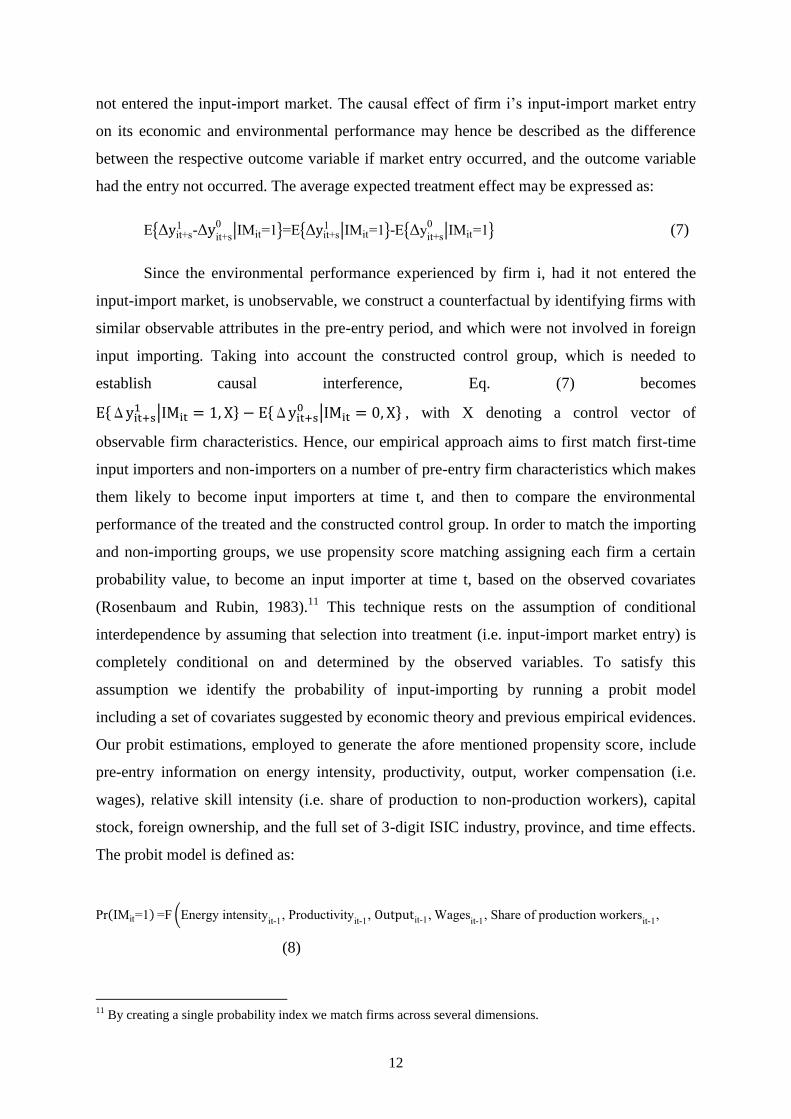
not entered the input-import market. The causal effect of firm i’s input-import market entry

on its economic and environmental performance may hence be described as the difference

between the respective outcome variable if market entry occurred, and the outcome variable

had the entry not occurred. The average expected treatment effect may be expressed as:

E{Δyit+s1 -Δy

it+s

0|IMit=1}=E{Δyit+s

1 |IMit=1}-E{Δyit+s

0|IMit=1} (7)

Since the environmental performance experienced by firm i, had it not entered the

input-import market, is unobservable, we construct a counterfactual by identifying firms with

similar observable attributes in the pre-entry period, and which were not involved in foreign

input importing. Taking into account the constructed control group, which is needed to

establish causal interference, Eq. (7) becomes

E{Δyit+s1 |IMit = 1, X} − E{Δyit+s

0 |IMit = 0, X} , with X denoting a control vector of

observable firm characteristics. Hence, our empirical approach aims to first match first-time

input importers and non-importers on a number of pre-entry firm characteristics which makes

them likely to become input importers at time t, and then to compare the environmental

performance of the treated and the constructed control group. In order to match the importing

and non-importing groups, we use propensity score matching assigning each firm a certain

probability value, to become an input importer at time t, based on the observed covariates

(Rosenbaum and Rubin, 1983).11

This technique rests on the assumption of conditional

interdependence by assuming that selection into treatment (i.e. input-import market entry) is

completely conditional on and determined by the observed variables. To satisfy this

assumption we identify the probability of input-importing by running a probit model

including a set of covariates suggested by economic theory and previous empirical evidences.

Our probit estimations, employed to generate the afore mentioned propensity score, include

pre-entry information on energy intensity, productivity, output, worker compensation (i.e.

wages), relative skill intensity (i.e. share of production to non-production workers), capital

stock, foreign ownership, and the full set of 3-digit ISIC industry, province, and time effects.

The probit model is defined as:

Pr(IMit=1) =F (Energy intensityit-1

, Productivityit-1

, Outputit-1, Wagesit-1

, Share of production workersit-1

, Capitalit-1

, Foreign ownershipit-1

,time, industry, province)

(8)

11

By creating a single probability index we match firms across several dimensions.

13

Predicting the probability of input-import market entry, the probit estimations are also

used to obtain the firm-level propensity scores. All firms i that become an input-importer are

then matched to a similar non-importing firm j based on these propensity scores.12

The

method chosen for selecting the appropriate match is the nearest neighbour caliper matching

method, where the minimum distance in terms of the calculated propensity scores is smaller

than a pre-specified value (i.e. caliper).13

We further limit the possibilities of matching to the

space of common support restricting the selection into similar treated and untreated firms to

the area between the lowest and highest propensity scores that fall in the propensity score

distribution for both of the respective groups.14

The chosen matching algorithm assigns only

one neighbour to each of the treated firms based on their proximity in calculated propensity

scores. Upon the identification of the matched pairs, we ensure the validity of the matching

exercise by analysing whether the pre-entry firm characteristics of the treated and the control

group are sufficiently similar (Caliendo and Kopeinig, 2008). To test for pre-treatment

similarity we examine whether treatment and control group differences are statistical

significant (balancing property test). Following Blundell and Costa Dias (2000) we use a

difference-in-difference strategy which contrasts growth rates of both treated and control

group firms. The advantage of this approach is that it allows us to account for additional

unobserved, time-constant factors that may influence firm performance. Moreover, we

compare firm performance across the entry and first three post entry periods. The

performance indicators are measured in growth relative to the pre-entry period (i.e. the period

before switching the trading status).

3.2 Data and sample characteristics

Annex Tables 1 and 2 provide a detailed overview over the main variables used in the

analysis, and provide some summary statistics. In this section we report the most salient

features of the dataset. We use microeconomic firm-level data from the Indonesian

Manufacturing Census, which includes information on around 48,000 different firms,

12

When defining the control group of non-importers we focus on firms that never imported during the whole

sample period. The treatment group, on the other hand, includes firms that imported for at least two consecutive

time periods, and that did not import before (import) market entry. When looking at firms that imported at least

for three consecutive periods we obtain qualitatively similar results for our main variables of interest. These

results are available upon request. 13

In case there is no control-group match for a treated firm for which the propensity score distance is smaller

than the specified caliper, the respective treated firm is excluded from the sample. 14

We allow non-importers to be selected more than once as an appropriate match for an input-importing firm.

14

covering the period 1991 to 2005. The manufacturing census categorises firms into HS 5-

digit ISIC Rev. 2 industries and is published by the Indonesian Statistical Agency (Badan

Pusat Statistic, BPS).15

The Indonesian Manufacturing Survey is an annual census of all

manufacturing firms with at least 20 employees and includes plant-level information on

output, intermediate inputs, labour, capital, foreign ownership, exports and imports and

energy consumption. Price deflators were used for all output, input and investment data,16

and

capital stocks were calculated based on a perpetual inventory method and using depreciation

rates from Arnold and Javorcik (2009).17

Environmental performance is defined as a firm’s

energy intensity (i.e. energy consumption over total output),18

while total factor productivity

has been calculated using the Levinsohn and Petrin (2003) methodology. Based on Solow’s

(1957) growth decomposition model, it is assumed that a plant-level linearly homogeneous

production functions can be subdivided into the growth rates of the individual input factors

and the growth rate of an unexplained growth residual. Since the estimation of production

functions tends to suffer from simultaneity concerns, given that inputs tend to be chosen

based on an observed level of productivity we follow Levinsohn and Petrin (2003) and use

intermediate inputs as a proxy to unobserved productivity shocks.

Table 1: Importing status, import sourcing and ownership (1) (2) (3) (4) (5)

Total Foreign

ownership

Domestic

Private

ownership

Domestic

Public

ownership

Import

share

FORsh DOMPRIVsh DOMPUBsh IMPsh

Import-starters (IM) 0.074 0.081 0.757 0.163 0.191

Never-importers (NIM) 0.926 0.013 0.837 0.150 0

Notes: The values reported reflect mean values over the time period 1991 to 2005. Our final data sample

includes 1,512 different import starters, over the whole time period considered, and 20,303 non-input importers

(Column 1). Columns 2-4 indicate on average the firm-level capital shares owned by foreign, domestic-private

or domestic-public investors, respectively. Column 5 shows on average the firm-level import share of

intermediate inputs.

15

At the moment there are 33 Indonesian provinces, seven of which have been created since 2000.To ensure

consistency over the considered time horizon (i.e. 1995-2005) we re-grouped all newly created provinces back

to their original provinces, which resulted in 26 provinces considered in this study. The Manufacturing Census

does not include information on the province Sulawesi Barat. 16

We are grateful to Rodriguez-Pose et al. (2013) for providing us with the deflators. The authors constructed a

value-added deflator for input and output information including exports and intermediate imports, as well as an

investment price deflator for net investment flows. The value added deflator was constructed by dividing the

value added in current prices by the value added in 1995 prices, while the investment price deflator was

calculated by dividing current-priced gross capital formation by 1995 prices. 17

Arnold and Javorcik (2009) use 20% for transport equipment, 10% for machinery and equipment, and 3.3%

for buildings, while land is not depreciated. 18

Batrakova and Davies (2012), and Martin (2011), also use energy intensities as an indicator of firm level

environmental performance and argue that the use of energy is positively correlated with firm level pollution.

15

Table 1 provides some basic statistics on the distribution of import starters and their

never-importing counterparts included in our estimating sample.19

New input importers

account for around 7.4% of all firms in our dataset, and feature on average a foreign equity

holding of about 8.1 %. On average new input importers’ equity is to about 75.7% privately

owned, and to around 16.3% by the government. Input importers tend to import, on average,

19.1% of their inputs from abroad and source, on average, around 80.9% of all used inputs

domestically.

Table 2 reports some basic firm characteristics of import-starters and non-importers.

Input importers are shown to be less energy intensive and more productive compared to the

group of non-input importing firms. Moreover, foreign input market entrants are also found

to be larger, in terms of both output and employment, and to pay higher wages.

Table 2: Input importer versus non-input importer firm characteristics (1) (2) (3) (4) (5)

Energy

intensity Productivity Output Employment

Wages

ln(ε) ln(𝜑) ln(𝑞𝑦) ln (𝐿) ln(𝑤)

Import-starters (IM) 0.93 6.34 21.67 5.07 13.19

Never-importers (NIM) 1.09 5.56 19.67 3.92 11.54

Notes: Table 2 reports mean values over the time period 1991 to 2005. The number of import starters in our

sample amounts to 1,512, while the number of never-importers amounts to 20,303. Energy intensity is defined

as total energy consumption over total output, while productivity is defined as total factor productivity based on

calculations using the Levinsohn and Petrin (2003) methodology. All monetary values are expressed in local

currency and have been deflated using a value added deflator. All values are expressed in log.

4. Empirical results

4.1 Foreign input market entry, firm productivity and energy intensity

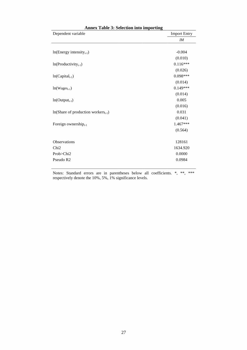
To identify pre-importing firm characteristics which determine the probability to enter

foreign input markets, we run a probit model measuring the selection into input importing in

year t based on firm characteristics in year t-1, as illustrated in Eq. (8).20

The estimation

outcome in Annex Table 3 shows no evidence for less energy-intensive firms self-selecting

into input importing. However, we find that more productive firms self-select to become

input importers. This is in line with some earlier evidence providing support for the

19

The reported statistics are expressed in means over the considered time horizon. 20

The specification and setting up of the probit model has been guided by economic theory as well as by

considerations of specification quality when using propensity score matching techniques.

16

hypothesis that firm productivity has a positive effect on the decision to import (Vogel and

Wagner, 2010; Castellani et al., 2010).21

The results also show that firms that are more

capital-intensive and skill-intensive (in terms of higher wages, but not in terms of lower share

of production to non-production workers) are characterised by a higher probability to source

inputs from abroad. In addition, the regression results also suggest that foreign-owned firms

are more likely to start importing, confirming that they are more likely to outsource their

intermediate inputs through their multinational network.

These probit estimations are used to obtain the firm-level propensity scores required

for matching our constructed treated group with the related control group, and the results of

the balancing property test, aimed at evaluating the quality of the matching are reported in

Annex Table 4. They confirm that for each of the treated group, a control group has been

identified with similar pre-treatment firm characteristics (i.e. the mean differences in the

variables introduced to calculate the propensity scores between the two groups are

statistically not significant).

Table 3 reports the findings for the post-entry effects. To establish the consequences

of importing on energy intensity and a series of alternative firm characteristics we compare

the outcome variables of matched importers and non-importers as illustrated in section 3.1.22

The change in energy intensity is reported to be some 11.6% smaller in the entry year than in

the time period before, having controlled for energy intensity changes of firms that did not

begin to import. There is also evidence for the persistency of this entry effect of up to two

years following the decision to import, bringing about a decline in energy intensity of up to

some 14.1 percentage points two years following import market entry. These findings hence

suggest a positive link between the ability to access intermediate input markets and firm-level

energy efficiency, and may point to a beneficial effect of an increasing integration of

intermediate input markets on the environment.

21

While Vogel and Wagner (2010) analyse importing activities and firm productivity for a selection of German

firms, Castellani et al. (2010) examine the productivity importing nexus for a sample of Italian firms. 22

We acknowledge the possibility that a shock in unobserved firm characteristics may affect input import

market participation, as well as firm-level environmental and economic outcomes.

17

Table 3: Post entry energy intensity effects: Difference in difference analysis of new input

importers and non-importers for the matched sample of firms

(1) (2) (3) (4) (5)

Dependent variable

(growth)

Energy

intensity Productivity Output Employment Wages

ln(ε) ln(𝜑) ln(𝑞𝑦) ln (𝐿) ln(𝑤)

Entry effect -0.116** 0.220*** 0.434*** 0.222*** 0.368***

(0.057) (0.052) (0.088) (0.058) (0.103)

1st year of importing -0.102** 0.272*** 0.368*** 0.137*** 0.252***

(0.048) (0.050) (0.044) (0.023) (0.050)

2nd year of importing -0.141*** 0.257*** 0.378*** 0.120*** 0.327***

(0.048) (0.053) (0.047) (0.024) (0.056)

3rd year of importing -0.062 0.232*** 0.346*** 0.137*** 0.350***

(0.052) (0.055) (0.050) (0.026) (0.061)

Notes: Standard errors are in parentheses below all coefficients. *, **, *** respectively denote the 10%, 5%,

1% significance levels.

Table 3 further shows that input import market entry also tends to be associated with positive

productivity, employment, output and wage growth premiums. Statistically significant

evidence is found for total factor productivity growth in the entry period, as well as in the

first, second and third period following market entry, with additional productivity premiums

of up to some 27% (in the year following market entry). Positive employment effects are

shown to be economically relevant from the period of market entry up until three years

following the decision to access foreign intermediate goods markets. The results reported in

Table 3 also point to a positive and highly persistent impact of the decision to import on

output and real wage growth, for importing firms relative to their never-importing

counterparts.

4.2 Robustness checks

Input market exposure, exporting and FDI

In the context of previous empirical studies, which find that learning and competition

effects are most likely to occur for firms’ most involved in exporting activities (cf.

Greenaway and Kneller, 2008; Damijan et al., 2007; Castellani, 2002), we also investigate

whether the extent of foreign input market exposure matters for firm-level energy intensity

and total factor productivity. We consider the level of exposure to foreign intermediate input

markets as an essential driver of firm level efficiency gains. We hence combine foreign input

market entry with a significant input-import share indicator variable taking the value one if

18

the imported total input ratio assumes values above the 25th

percentile. The results

complement previous findings on the exposure to export markets, as they show a significant

growth premium in energy efficiency upon beginning to import (Column 1, Table 4), and a

substantial gain in total factor productivity following the decision to import (Column 2, Table

4). The effects on energy and total factor efficiency are in magnitude significantly larger than

those reported in our baseline specifications in Table 3 (Columns 1 and 2).

In light of the strong focus on exporting status and environmental performance in

previous firm-level studies (cf. Galdeano-Gomez, 2010; Girma et al., 2008; Batrakova and

Davis, 2012), and to address the potential concern that our results may be driven by firm

exports rather than imports, we reduce the firm total population to the sub-sample of non-

exporting firms - i.e. we contrast non-exporting importers with firms that neither imported

nor exported (i.e. never-traders), over the considered time. The estimation results reported in

Table 4 (Column 3) tend to confirm previous findings as the parameter estimates for the

entry, as well as first and second post-entry periods are statistically highly significant at the

usual thresholds, however at somewhat reduced magnitudes (showing values of -0.010, -

0.018 and -0.015, respectively). These findings suggest a significant but reduced impact on

energy efficiency for firms that only import intermediates and do not export at the same time.

Regarding total factor productivity growth, the results reported in Table 4 (Column 4) also

point to a statistically significant premium for pure input importers when contrasting them to

their never-trading counterparts, although at slightly smaller magnitudes (relative to your

baseline estimations).

Table 4: Post entry effects: Input market participation , Exporting, FDI

Foreign input market

participation (25%)

Non-exporting input

importers

Non-FDI & non-exporting

importers

(1) (2)

(3) (4)

(5) (6)

Dependent variable

(growth)

Energy

intensity Productivity

Energy

intensity Productivity

Energy

intensity Productivity

ln(ε) ln(𝜑) ln(ε) ln(𝜑) ln(ε) ln(𝜑)

Entry effect -0.143** 0.279***

-0.010** 0.212***

-0.005 0.229***

(0.071) (0.065)

(0.006) (0.077)

(0.005) (0.077)

1st year of importing -0.161*** 0.363***

-0.018*** 0.142**

-0.023*** 0.146**

(0.063) (0.066)

(0.004) (0.078)

(0.008) (0.077)

2nd year of importing -0.172*** 0.343***

-0.015*** 0.222***

-0.018** 0.237***

(0.063) (0.068)

(0.004) (0.085)

(0.008) (0.082)

3rd year of importing -0.107*** 0.250***

-0.010 0.0756

-0.005* 0.164

(0.063) (0.070)

(0.008) (0.091)

(0.006) (0.087)

Notes: Standard errors are in parentheses below all coefficients. *, **, *** respectively denote the 10%, 5%, 1%

significance levels.

19

Accounting for the possibility that foreign-owned firms may gain easier access to

foreign produced intermediate inputs through their multinational networks, and may benefit

from a direct transfer of better and more environmentally-friendly technologies by their

parent companies, we additionally aim to clean the import premium from both exporting and

FDI status. We thus compare non-exporting and non-foreign owned import starters with non-

foreign owned never-traders. The results, presented in Table 4 (Column 5), confirm the

significant positive relationship between energy efficiency and import-status also for purely

domestically-owned firms (for the post-entry periods), but show, in magnitude, a significantly

smaller effect of input-import status on firm-level energy efficiency growth, compared to our

main findings in Table 3. This may, indeed, point to an important influence of foreign direct

investment on the impact of input importing, and may support existing findings in favour of a

positive effect of foreign ownership on environmental firm performance in the host country

(Albornoz et al., 2009; Cole et al. 2006, 2008; Kaiser and Schulze, 2003). As for the growth

in total factor productivity, the results in Table 4 (Column 6) confirm, by and large, our

baseline findings showing statistically significant import premiums for the entry, first and

second post entry periods.

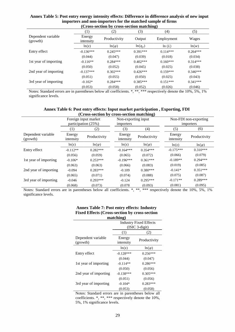
Alternative matching approach

In addition to the pooled matching technique reported above, we also implement the

matching on a cross-section by cross-section basis, and hence require the matching algorithm

to select matches that occur in the same time period. This reduces the risk of comparing firms

that had to deal with remarkably different macroeconomic conditions. After the selection of

matched pairs of treated and untreated firms we pool these observations to construct a panel

dataset that we use for our analysis.

As in the previous section, we use a difference-in-difference strategy following

Blundell and Costa Dias (2000), and we compare firm performance across the entry and first

three post entry periods. The results are reported in Annex Tables 5 and 6, and by and large

confirm our previous findings. The former table shows that switching import status leads to a

lower energy intensity growth of about 13.6% in the market entry year compared to the

period before; this effect persists also in the three years following import market entry,

although at different levels of magnitude.23

These findings corroborate the hypothesis that the

23

For the1st, 2

nd, and 3

rd post entry periods our results show lower energy intensities of around 11.6%, 13.7%,

and 10.2%, respectively, relative to the pre-entry period.

20

ability to access intermediate input markets and to integrate into international supply chains

may have a positive effect on company-level energy efficiency.24

Moreover, using the cross-section-by-cross section firm matching strategy provides

further support for positive productivity, output, employment, and wage growth premiums.

Our findings show statistically highly significant coefficients for total factor productivity

growth in the entry, and the first three periods following market entry, with an additional

productivity increase of up to some 30% (in the second year following market entry),

compared to the pre-entry period. Positive and highly persistent premiums are also reported

for new input importers’ size growth (in terms of both output and employment) for the period

of market entry up until three years following the decision to access foreign intermediate

goods markets. The results reported in Annex Table 5 also point to a positive and statistically

significant impact of the decision to import on real wages growth, for importing firms relative

to their never-importing counterparts.

Turning to the impact of a higher exposure to foreign input markets on learning,

competition, and hence productivity and energy intensity, but also to take into account effects

linked to exporting and foreign direct investment, we repeat the above sensitivity analysis

when employing cross-section-by-cross-section matching. The results for firms that import

more inputs from abroad are reported in Annex Table 6 (columns 1 and 2). They show

statistically significant coefficients for energy intensity for the entry and first post entry

period. Regarding total factor productivity, the coefficients are statistically highly significant

and are, on average, of a similar magnitude compared to the baseline results shown in Annex

Table 5. Excluding exporting firms from the sample (Annex Table 6, columns 3 and 4)

confirms these results for energy intensity, showing coefficients whose magnitude even

exceeds those of the baseline specification. Dropping exporters from the sample, however,

also results in still highly significant and, in magnitude, slightly larger productivity

premiums. Finally, the findings are also robust to the exclusion of exporters and foreign-

owned (i.e. FDI) firms, showing statistically significant energy intensity and productivity

growth parameter estimates for all periods (columns 5 and 6).

24

To control for the possibility that our findings may be driven by individual industry characteristics we also

include industry fixed effects at the ISIC 3-digit level in a separate set of cross-section by cross-section

regressions. The intuition behind this is that some sectors might be relatively more energy-intensive or subject to

a higher number of energy-saving environmental policies than other sectors. Annex table 7 reports the results for

the energy intensity and productivity variable and shows very similar parameter estimates compared to our

baseline specification.

21

5. Conclusions

A main concern over international trade and increasing global market integration is its

impact on the environment. This is particularly true and important for developing nations,

where presumably lower environmental standards have been linked to adverse environmental

effects and increasing pollution. This paper contributes to this debate by focusing on the link

between participation in foreign intermediate goods markets and firm-level environmental

performance in a developing country.

The theoretical and empirical findings in this paper demonstrate significant evidence that

imported intermediate goods enhance firms' economic efficiency with an important positive

effect on environmental performance. Our results show that by switching from being a non-

input importer to an input importer of foreign intermediate materials, a company is likely to

improve its economic efficiency and reduce its energy intensity. Our baseline estimates

indicate a positive effect of around 22.0% and 11.6% on economic efficiency and energy

efficiency growth, respectively, immediately upon entry, and a statistically significant and

persistently positive impact of around 25.7% and 14.1%, respectively, two years following

market entry. Our findings may hence carry important implications for both government

policies and firm level strategies, as they suggest that there are important economic and

environmental efficiency gains to be realised when enabling developing country producers to

gain access to foreign intermediate good markets. Our results may also be understood as a

call for more research on the trade – environment nexus, in particular regarding the effect of

importing intermediate inputs on a firm’s propensity to directly invest in cleaner

technologies.

22

REFERENCES

Amiti, M., Konings J., 2007, Trade Liberalization, Intermediate Inputs, and Productivity: Evidence

from Indonesia, American Economic Review, 97(5), 1611-1638.

Albornoz, F., Cole, M. A., Elliott, R. J. R., Ercolani, M. G., 2009, In search of environmental

spillovers, The World Economy, 32(1), 136–163.

Antweiler, W., Copeland, B. R., Taylor, M. S., 2001, Is free trade good for the environment? The

American Economic Review, 91(4), 877–908.

Arnold, M. J., Javorcik, B. S., 2009, Gifted kids or pushy parents? Foreign direct investment and plant

productivity in Indonesia, Journal of International Economics, 79(1), 42-53.

Barrett, S., 1994, Strategic environmental policy and international trade, Journal of Public

Economics, 54(3), 325–338.

Batrakova, S., Davies, R. B., 2012, Is there an environmental benefit to being an exporter? Evidence

from firm-level data, Review of World Economics, 148(3), 449-474.

Bernard, A. B., Redding, S. J., Schott, P. K., 2007, Comparative advantage and heterogeneous firms,

The Review of Economic Studies, 74(1), 31–66.

Blundell, R., Dias, M. C., 2000, Evaluation methods for non-experimental data, Fiscal Studies, 21(4),

427–468.

Castellani, D., 2002, Export behaviour and productivity growth: Evidence from Italian manufacturing

firms, Weltwirtschaftliches Archiv, 138, 605–628.

Castellani, D., Serti, F., Tommasi, C., 2010, Firms in International Trade: Importers and Exporters

Heterogeneity in the Italian Manufacturing Industry, The World Economy, 33(3), 424-457.

Cole, M. A., Elliott, R. J. R., Strobl, E., 2008, The environmental performance of firms: The role of

foreign ownership, training, and experience, Ecological Economics, 65(3), 538–546.

Copeland, B. R., Taylor, M. S., 1994, North-south trade and the environment, The Quarterly Journal

of Economics, 109(3), 755–787.

Copeland, B. R., Taylor, M. S., 1997, A simple model of trade, capital mobility, and the environment,

NBER Working Paper No. 5898, Cambridge, MA: National Bureau of Economic Research.

Damijan, J., Polanec, S., Prasnikar, J., 2007, Outward FDI and productivity: Micro evidence for

Slovenia, The World Economy, 30, 135–155.

Dean, J. M., Lovely, M. E., 2010, Trade growth, production fragmentation, and China’s environment.

In: R. Feenstra, & S.-J. Wei (Eds.), China’s growing role in world trade, (Chapter 11 pp. 429–474).

Chicago: University of Chicago Press.

Eskeland, G. S., Harrison, A. E., 2003, Moving to greener pastures? Multinationals and the pollution

haven hypothesis, Journal of Development Economics, 70(1), 1–23.

Ethier, W. J., 1982, National and international returns to scale in the modern theory of international

trade, American Economic Review, 72 (3), 389–405.

Galdeano-Gomez, E., 2010, Exporting and environmental performance: A firm-level productivity

analysis, The World Economy, 33(1), 60–88.

Gibson, Mark J., Graciano, T.A., 2011, The Decision to Import, American Journal of Agricultural

Economics, 93(2), 444-449.

23

Girma, S., Hanley, A., Tintelnot, F., 2008, Exporting and the environment: A new look with

microdata (Kiel Working Paper No. 1423). Kiel: Kiel Institute for the World Economy.

Goldberg, P. K., Khandelwal A. K., Pavcnik N., Topalova P., 2010, Imported Intermediate Inputs and

Domestic Product Growth: Evidence from India, The Quarterly Journal of Economics, 125(4), 1727-

1767.

Greenaway, D., Kneller, R., 2008, Exporting, productivity and agglomeration, European Economic

Review, 52, 919-939.

Grossman, G.M., Helpman, E., 1991, Innovation and Growth in the Global Economy, MIT Press,

Cambridge, MA.

Heckman, J. J., Ichimura, H., Todd, P. E., 1997, Matching as an econometric evaluation estimator:

Evidence from evaluating a job training programme, The Review of Economic Studies, 64(4), 605-

654.

Imbruno, M., 2014, Trade Liberalization, Intermediate Inputs and Firm Efficiency: Direct versus

Indirect Modes of Import, Discussion Papers 2014-02, University of Nottingham, GEP.

Kaiser, K., Schulze, G.G., 2003, International competition and environmental expenditures: Empirical

evidence from Indonesian manufacturing plants, HWWA Discussion Paper 222, Hamburg: Hamburg

Institute of International Economics.

Kasahara, H., Rodrigue, J., 2008, Does the use of imported intermediates increase productivity? Plant-

level evidence, Journal of Development Economics, 87(1), 106-118.

Khandelwal, A., Topalova, P., 2011, Trade Liberalization and Firm Productivity: The

Case of India, The Review of Economics and Statistics, 93(3), 995-1009.

Krugman, P.. 1980. Scale Economies, Product Differentiation, and the Pattern of Trade, American

Economic Review, 70 (5), 950-59.

Larch, M., and Wanner J., 2014. Carbon Tariffs: An Analysis of the Trade, Welfare and Emission

Effects, CESifo Working Paper Series 4598, CESifo Group Munich.

Levinsohn, James, Petrin, Amil, 2003. Estimating production functions using inputs to control for

unobservables, Review of Economic Studies, 70, 317-341.

Levinson, A., 2009, Technology, international trade, and pollution from US manufacturing, American

Economic Review, 99(5), 2177-2192.

Markusen, J. R., 1989, Trade in Producer Services and in Other Specialized Intermediate Inputs,

American Economic Review, 79(1), 85.95.

Markusen, J. R., Morey, E. R., Olewiler, N., 1995, Competition in regional environmental policies

when plant locations are endogenous, Journal of Public Economics, 56(1), 55–77.

Martin, L., 2011, Energy efficiency gains from trade: greenhouse gas emissions and India’s

manufacturing sector, Melbourne University Working Paper.

McGuire, M. C., 1982, Regulation, factor rewards, and international trade, Journal of Public

Economics, 17(3), 335–354.

Melitz, M.J., 2003, The impact of trade on intra-industry reallocations and aggregate industry

productivity, Econometrica, 71(6), 1695-1725.

Melitz, M.J., Ottaviano, G.I.P., 2008, Market Size, Trade, and Productivity, Review of Economic

Studies, 75(1), 295-316.

Olley, S., Pakes, A., 1996. The dynamics of productivity in the telecommunications equipment

industry, Econometrica, 65(1), 292-332.

24

Pethig, R., 1976, Pollution, welfare, and environmental policy in the theory of comparative advantage.

Journal of Environmental Economics and Management, 2(3), 160-169.

Popp,D., 2011, International Technology transfer, climate change, and the clean development

mechanism, Review of Environmental Economics and Policy, 5, 131-152.

Rodríguez-Pose, A., Tselios, V., Winkler, D., Farole, T., 2013, Geography and the Determinants of

Firm Exports in Indonesia, World Development, 44: 225-240

Romer, P., 1990. Endogenous technological change, Journal of Political Economy, 98 (5), 71-102.

Rosenbaum, P. R., Rubin, D. B., 1983, The central role of the propensity score in observational

studies for causal effects, Biometrika, 70(1), 41-55.

Schor, A., 2004, Heterogeneous productivity response to tariff reduction. Evidence from Brazilian

manufacturing firms, Journal of Development Economics, 75(2), 373-396.

Stern, N., 2007, The Economics of Climate Change: The Stern Review, Cambridge:

Cambridge University Press.

Solow, R., M., 1957, Technical change and the aggregate production function, Review of Economics

and Statistics, 39(3), 312–320.

Vogel, A., Wagner J., 2010, Higher Productivity in Importing German Manufacturing Firms: Self-

selection, Learning from Importing or Both? The World Economy, 145(4), 641-665.

25

ANNEX

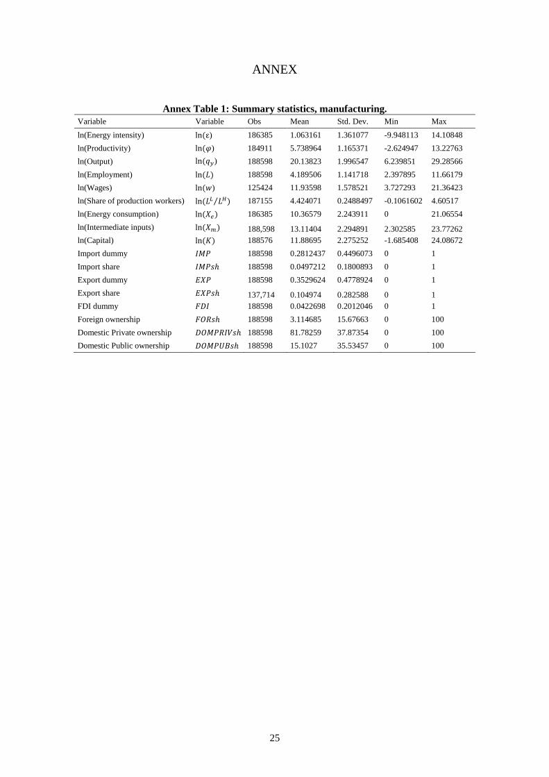
Annex Table 1: Summary statistics, manufacturing.

Variable Variable Obs Mean Std. Dev. Min Max

ln(Energy intensity) ln(ε) 186385 1.063161 1.361077 -9.948113 14.10848

ln(Productivity) ln(𝜑) 184911 5.738964 1.165371 -2.624947 13.22763

ln(Output) ln(𝑞𝑦) 188598 20.13823 1.996547 6.239851 29.28566

ln(Employment) ln(𝐿) 188598 4.189506 1.141718 2.397895 11.66179

ln(Wages) ln(𝑤) 125424 11.93598 1.578521 3.727293 21.36423

ln(Share of production workers) ln(𝐿𝐿 𝐿𝐻)⁄ 187155 4.424071 0.2488497 -0.1061602 4.60517

ln(Energy consumption) ln(𝑋𝑒) 186385 10.36579 2.243911 0 21.06554

ln(Intermediate inputs) ln(𝑋𝑚) 188,598 13.11404 2.294891 2.302585 23.77262

ln(Capital) ln(𝐾) 188576 11.88695 2.275252 -1.685408 24.08672

Import dummy 𝐼𝑀𝑃 188598 0.2812437 0.4496073 0 1

Import share 𝐼𝑀𝑃𝑠ℎ 188598 0.0497212 0.1800893 0 1

Export dummy 𝐸𝑋𝑃 188598 0.3529624 0.4778924 0 1

Export share 𝐸𝑋𝑃𝑠ℎ 137,714 0.104974 0.282588 0 1

FDI dummy 𝐹𝐷𝐼 188598 0.0422698 0.2012046 0 1

Foreign ownership 𝐹𝑂𝑅𝑠ℎ 188598 3.114685 15.67663 0 100

Domestic Private ownership 𝐷𝑂𝑀𝑃𝑅𝐼𝑉𝑠ℎ 188598 81.78259 37.87354 0 100

Domestic Public ownership 𝐷𝑂𝑀𝑃𝑈𝐵𝑠ℎ 188598 15.1027 35.53457 0 100

26

Annex Table 2: Definition of firm-level variables

Variable Variable Description

Energy intensity 𝜀 Total electricity and fuel purchased standardised by total output (i.e.

Energy-Output ratio).

Productivity 𝜑 Total Factor Productivity (TFP) as defined by Levinsohn and Petrin

(2003).

Output 𝑞𝑦 Total value of all goods produced in any given year.

Employment 𝐿 Total number of workers (paid and unpaid)

Wages 𝑤 Real total compensation of production and non-production workers

Share of production

workers 𝐿𝐿 𝐿𝐻⁄ Employment share of production to non-production workers.

Energy consumption 𝑋𝑒 Total electricity and fuel purchased as reported by Indonesian firms to

BPS.

Intermediate inputs

consumption 𝑋𝑖𝑛𝑡

Total consumption in intermediate inputs, (including both Materials

(Xm) and energy consumption (Xe).

Capital 𝐾

Capital stocks calculated on the basis of the perpetual inventory method

using depreciation rates of 20%, 10%, and 3.3% for transport

equipment, machinery and equipment, and for buildings, respectively.

Land is not depreciated.

Import dummy 𝐼𝑀𝑃 Indicator variable taking the value one if a particular firm imported at

some point over the considered time horizon; and zero otherwise.

Import share 𝐼𝑀𝑃𝑠ℎ Inputs imported (as % of total intermediate consumption)

Export dummy 𝐸𝑋𝑃 Indicator variable taking the value one if a particular firm exported at

some point over the considered time horizon; and zero otherwise.

Export share 𝐸𝑋𝑃𝑠ℎ Export sales (as % of total output)

FDI dummy 𝐹𝐷𝐼 Indicator variable taking the value one, if a firm is foreign owned (i.e. if

a foreign company owns at least 10% of the firm's equity).

Foreign ownership 𝐹𝑂𝑅𝑠ℎ Percentage of firm assets owned by a foreign investor.

Domestic Private

ownership 𝐷𝑂𝑀𝑃𝑅𝐼𝑉𝑠ℎ Percentage of firm assets owned by a domestic private investor.

Domestic Public

ownership 𝐷𝑂𝑀𝑃𝑈𝐵𝑠ℎ Percentage of firm assets owned by the government.

Import-starter dummy

(Treated group)

𝐼𝑀

Indicator variable taking the value one if a firm switched from being a

non-importer to being an importer. When we use matching techniques

input-importers are identified as firms that switch to and stay input-

importer: i.e. firms that do not import intermediates two years prior to

switching to importing, and then import for at least 2 years.

Never-importer dummy

(Untreated group) 𝑁𝐼𝑀

Indicator variable taking the value one if a firm never imports along the

entire sample period.

27

Annex Table 3: Selection into importing Dependent variable

Import Entry

IM

ln(Energy intensityt-1)

-0.004

(0.010)

ln(Productivityt-1)

0.116***

(0.026)

ln(Capitalt-1)

0.098***

(0.014)

ln(Wagest-1)

0.149***

(0.014)

ln(Outputt-1)

0.005

(0.016)

ln(Share of production workerst-1)

0.031

(0.041)

Foreign ownershipt-1

1.467***

(0.564)

Observations

128161

Chi2

1634.920

Prob>Chi2

0.0000

Pseudo R2

0.0984

Notes: Standard errors are in parentheses below all coefficients. *, **, ***

respectively denote the 10%, 5%, 1% significance levels.

28

Annex Table 4: Quality of propensity score matching: T-tests comparing sample means of the treated and control groups

ln(Energy intensity) ln(Productivity) ln(Output)

Treated Control

T-test

(stat.)

T-test

(p-

value)

Treated Control T-test

(stat.)

T-test

(p-

value)

Treated Control T-test

(stat.)

T-test

(p-

value)

ln(Energy intensityt-1) -3.658 -3.680 0.410 0.682 -3.678 -3.717 0.710 0.480 -3.667 -3.702 0.650 0.518

ln(Productivityt-1) -5.234 -5.313 1.540 0.124 -5.223 -5.294 1.370 0.169 -5.233 -5.304 1.390 0.166

ln(Capitalt-1) 0.460 0.397 0.930 0.350 0.425 0.357 1.010 0.312 0.451 0.392 0.880 0.380

ln(Wagest-1) 13.124 13.017 1.570 0.116 13.131 12.987 2.020 0.110 13.122 13.018 1.530 0.126

ln(Outputt-1) 14.729 14.626 1.190 0.236 14.731 14.596 1.500 0.135 14.725 14.635 1.040 0.300

ln(Share non-

production workerst-1) -7.136 -7.129 -0.600 0.549 -7.134 -7.128 -0.460 0.645 -7.135 -7.125 -0.870 0.386

Foreign ownershipt-1 0.006 0.006 -0.880 0.380 0.006 0.006 -0.910 0.362 0.006 0.007 -1.200 0.231

Notes: Standard errors are in parentheses below all coefficients. *, **, *** respectively denote the 10%, 5%, 1% significance levels. All

model specifications include ISIC 4-digit industry and time effects. P-values are reported for the respective t-tests.

Annex Table 4: continued.

ln(Employment) ln(Wages)

Treated Control

T-test

(stat.)

T-test

(p-

value)

Treated Control T-test

(stat.)

T-test

(p-

value)

ln(Energy intensityt-1) -3.662 -3.702 0.730 0.464 -3.537 -3.535 -0.020 0.984

ln(Productivityt-1) -5.231 -5.300 1.350 0.176 -5.151 -5.237 1.200 0.232

ln(Capitalt-1) 0.451 0.392 0.890 0.372 0.454 0.434 0.210 0.833

ln(Wagest-1) 13.130 13.028 1.490 0.136 13.270 13.121 1.480 0.139

ln(Outputt-1) 14.733 14.647 0.990 0.320 15.003 14.782 1.810 0.071

ln(Share non-production

workerst-1) -7.133 -7.125 -0.710 0.477 -7.134 -7.133 -0.070 0.947

Foreign ownershipt-1 0.006 0.007 -1.150 0.249 0.005 0.006 -0.570 0.571

Notes: see above.

29

Annex Table 5: Post entry energy intensity effects: Difference in difference analysis of new input

importers and non-importers for the matched sample of firms

(Cross-section by cross-section matching)

(1) (2) (3) (4) (5)

Dependent variable

(growth)

Energy

intensity Productivity Output Employment Wages

ln(ε) ln(𝜑) ln(𝑞𝑦) ln (𝐿) ln(𝑤)

Entry effect -0.136*** 0.245*** 0.391*** 0.114*** 0.264***

(0.044) (0.047) (0.039) (0.018) (0.034)

1st year of importing -0.116** 0.284*** 0.402*** 0.160*** 0.314***

(0.050) (0.052) (0.045) (0.025) (0.038)

2nd year of importing -0.137*** 0.302*** 0.426*** 0.159*** 0.346***

(0.051) (0.055) (0.050) (0.025) (0.043)

3rd year of importing -0.102* 0.284*** 0.385*** 0.151*** 0.341***

(0.053) (0.058) (0.052) (0.026) (0.046)

Notes: Standard errors are in parentheses below all coefficients. *, **, *** respectively denote the 10%, 5%, 1%

significance levels.

Annex Table 6: Post entry effects: Input market participation , Exporting, FDI

(Cross-section by cross-section matching)

Foreign input market

participation (25%)

Non-exporting input

importers

Non-FDI non-exporting

importers

(1) (2)

(3) (4)

(5) (6)

Dependent variable

(growth)

Energy

intensity Productivity

Energy

intensity Productivity

Energy

intensity Productivity

ln(ε) ln(𝜑) ln(ε) ln(𝜑) ln(ε) ln(𝜑)

Entry effect -0.112** 0.282***

-0.164*** 0.354***

-0.175*** 0.310***

(0.056) (0.059)

(0.065) (0.072)

(0.066) (0.079)

1st year of importing -0.106* 0.253***

-0.196*** 0.361***

-0.189** 0.294***

(0.063) (0.063)

(0.066) (0.083)

(0.019) (0.085)

2nd year of importing -0.094 0.283***

-0.109 0.380***

-0.141* 0.351***

(0.065) (0.071)

(0.074) (0.088)

(0.075) (0.087)

3rd year of importing -0.046 0.293***

-0.124 0.295***

-0.171** 0.289***

(0.068) (0.073)

(0.078 (0.093)

(0.081) (0.095)

Notes: Standard errors are in parentheses below all coefficients. *, **, *** respectively denote the 10%, 5%, 1%

significance levels.

Annex Table 7: Post entry effects: Industry

Fixed Effects (Cross-section by cross-section

matching)

Industry Fixed Effects

(ISIC 3-digit)

(1) (2)

Dependent variable

(growth)

Energy

intensity Productivity

ln(ε) ln(𝜑)

Entry effect -0.128*** 0.256***

(0.044) (0.047)

1st year of importing -0.114** 0.286***

(0.050) (0.056)

2nd year of importing -0.138*** 0.305***

(0.051) (0.056)

3rd year of importing -0.104* 0.283***

(0.053) (0.058)

Notes: Standard errors are in parentheses below all

coefficients. *, **, *** respectively denote the 10%,

5%, 1% significance levels.