energy e cient code updates in wireless sensor...
TRANSCRIPT

Energy Efficient Code Updates inWireless Sensor Networks
Validation and enhancement of the GCP protocol
Peter FinderupRobertas Backys
Thomas Birk Abildgaard


Department of Computer Science
Aalborg University
Selma Lagerløfs Vej 300
9220 Aalborg
Phone 96 35 80 80
Fax 96 35 97 98
http://www.cs.aau.dk
Title:Energy Efficient Code Updates inWireless Sensor Networks- Validation and enhancement of theGCP protocol
Project Period:DAT6, spring semester 2010
Project Group:d617a
Participants:Peter FinderupRobertas BackysThomas Birk Abildgaard
Supervisor:Brian Nielsen
Circulation: 5
Number of pages: 98
Number of appendixes: 6 and 1 CD.
Finished on: 31th of May, 2010
Abstract:
Wireless Sensor Networks (WSNs) are typicallydeployed in scenarios where sensor measurementsfrom several distinct locations are needed. WSNsusually consist of many nodes scattered aroundan environment, often one humans tend to avoid.Example of hard to reach or hostile environmentscould be inside a glacier or upon a battlefield. Aproblem occurs once a WSN has been deployedand the running application needs a software up-date, either because errors has been found, para-meters are tweaked or application improvementsare needed. Collecting each sensor node by handwould be a tedious task, impractical if not im-possible. Therefore, when such sensors need tobe updated another approach is required.The lifetime of a WSN highly depends of theutilisation of the energy resource available. Theenergy supply of the individual sensor node is avery scarce resource, and the source of energy canseldom be replaced after deployment of the WSN.In this report we focus on energy efficient codeupdates in a WSN through wireless communica-tion. We systematic describe the Gossip-basedCode Propagation protocol and implement it.Through the specification of the GCP protocol wediscover ambiguous protocol description, as wellas limitations to the protocol.
We present an extension which incorporates a re-
liability mechanism which ensures updates can
happen though communication is faulty. We also
improve the utilisation of tokens which ensures a
better overall load balancing in dense networks.
As a conclusion, we compare our results from the
GCP and our extension to reason about their
performance while distributing code updates in
a WSN.
The contents of this report is freely available, however, publication (with source of reference) is only al-
lowed in agreement with the authors.

Preface
This report is written by group d617a as a DAT6 (master) project from February 1st
2010 to May 31th 2010 at the Department of Computer Science at Aalborg University.This report is addressed to other students, supervisors and anyone else who might beinterested in the subject. To read and understand the report correctly, it is necessary tohave knowledge about the most basic computer related terms.The entire report is written in English and no translation will be accessible, it is thereforerequired to understand English. Abbreviations and acronyms will at first appearance bewritten in parenthesis, to avoid breaking the reading stream. Specification of gender inthis report is not to be understood as suppression or any other form of political/religiousposition. The gender is only specified to simplify the process of writing for the authors.References to sources are marked by [#], where # refers to the related literature in thebibliography at the end of the report.The Appendixes to this report is found in the last chapter of the report.The report is written in LATEX and are accessible as a PDF-document, which can be readwith Adobe Acrobat Reader.Finally, the group will like to thank our supervisor Brian Nielsen who has supported usthroughout this project.
Content of the CD
• Graph folder with all graphs.
• Source folder with our source files.
• Simulation date.
Thomas Abildgaard Robertas Backys
Peter Finderup
iii


Contents
1 Introduction 1
1.1 Challenges . . . . . . . . . . . . . . . . . . . . . . . . . . . . . . . . . . . . 1
1.2 Motivation . . . . . . . . . . . . . . . . . . . . . . . . . . . . . . . . . . . 2
1.3 Problem Statement . . . . . . . . . . . . . . . . . . . . . . . . . . . . . . . 3
1.4 Report structure . . . . . . . . . . . . . . . . . . . . . . . . . . . . . . . . 3
2 Background on wireless sensor networks 4
2.1 Typical hardware platforms . . . . . . . . . . . . . . . . . . . . . . . . . . 5
2.2 Update management model . . . . . . . . . . . . . . . . . . . . . . . . . . 8
2.3 Summary . . . . . . . . . . . . . . . . . . . . . . . . . . . . . . . . . . . . 10
3 GCP protocol specification 11
3.1 GCP Protocol . . . . . . . . . . . . . . . . . . . . . . . . . . . . . . . . . . 11
4 Verification of the GCP protocol 16
4.1 Initial GCP model . . . . . . . . . . . . . . . . . . . . . . . . . . . . . . . 17
4.2 Timing analysis . . . . . . . . . . . . . . . . . . . . . . . . . . . . . . . . . 20
4.3 Energy analysis . . . . . . . . . . . . . . . . . . . . . . . . . . . . . . . . . 26
4.4 Summary . . . . . . . . . . . . . . . . . . . . . . . . . . . . . . . . . . . . 29
5 Simulation of GCP 30
5.1 Introduction to NS2 . . . . . . . . . . . . . . . . . . . . . . . . . . . . . . 31
5.2 Implementation of GCP . . . . . . . . . . . . . . . . . . . . . . . . . . . . 34
5.3 Basic GCP tests . . . . . . . . . . . . . . . . . . . . . . . . . . . . . . . . 38
5.4 Simulation scenarios . . . . . . . . . . . . . . . . . . . . . . . . . . . . . . 39
5.5 GCP test results . . . . . . . . . . . . . . . . . . . . . . . . . . . . . . . . 44
5.6 Explanation for deviation . . . . . . . . . . . . . . . . . . . . . . . . . . . 48
5.7 Replicate results of GCP . . . . . . . . . . . . . . . . . . . . . . . . . . . . 50
5.8 Summary . . . . . . . . . . . . . . . . . . . . . . . . . . . . . . . . . . . . 52
6 Extension of the GCP protocol 53
6.1 Problems with the GCP protocol . . . . . . . . . . . . . . . . . . . . . . . 53
6.2 Specification of extension . . . . . . . . . . . . . . . . . . . . . . . . . . . 58
6.3 Implementation of eGCP . . . . . . . . . . . . . . . . . . . . . . . . . . . 62
6.4 Test of the extension . . . . . . . . . . . . . . . . . . . . . . . . . . . . . . 68
6.5 eGCP test results . . . . . . . . . . . . . . . . . . . . . . . . . . . . . . . . 70
6.6 Summary . . . . . . . . . . . . . . . . . . . . . . . . . . . . . . . . . . . . 73
7 Conclusion 74
7.1 Future work . . . . . . . . . . . . . . . . . . . . . . . . . . . . . . . . . . . 77
A Calculating average density 80
B UPPAAL models 82
B.1 UPPAAL model of the original GCP protocol . . . . . . . . . . . . . . . . 83
B.2 UPPAAL model of the original GCP protocol with a half duplex radio . . 84

B.3 UPPAAL model of the original GCP protocol with time and node connec-tivity . . . . . . . . . . . . . . . . . . . . . . . . . . . . . . . . . . . . . . . 85
B.4 UPPAAL model of the original GCP protocol with energy, time and nodeconnectivity . . . . . . . . . . . . . . . . . . . . . . . . . . . . . . . . . . . 86
B.5 Maple Time and Energy calculations . . . . . . . . . . . . . . . . . . . . . 87
C GCP results 88C.1 GCP simulation results - Scenario 1 . . . . . . . . . . . . . . . . . . . . . 89
D GCP Replication results 93
E eGCP results 95
F Report summary 97
vi

Chapter 1
Introduction
Today modern technology improves faster than ever before. The numbers of transistorsthat can fit a square inch increases each year and thus electronic devices get smaller andsmaller. This development is of great importance for sensor nodes since their actual sizecan determine if they can be applied in a specific area or not. An example could be anature habitat, where the miniaturisation of the sensor nodes allow us to collect data ina non intrusive manner. In this scenario tiny, almost invisible sensors become essentialin terms of getting accurate data without interfering with the normal life of the animalsor polluting the area.
Wireless sensor networks (WSNs) are typically deployed in scenarios where sensormeasurements from several distinct locations are needed. They usually consist of manynodes scattered around an environment, often one humans tend to avoid; either becauseits costly or too dangerous. Examples of such areas are at the bottom of the ocean, inspace, on a battlefield[8] or deep inside a glacier[15].
A problem occurs once a WSN has been deployed and the running application needsan software update, either because errors has been found, parameters are tweaked orapplication improvements are needed. Collecting each sensor node by hand would bea tedious task, impractical if not impossible. Therefore, when such sensors need to beupdated another approach is required.
In this report the focus will be on energy efficient code updates in a WSN throughwireless communication. However, several challenges arises when updating a sensornetwork wirelessly.
1.1 Challenges
There are many challenges when updating a wireless sensor network. Physical reachabi-lity can post a problem. Transmitting the update over an unstable media such as a radiois troublesome. The main problem with wireless sensor networks is power consumption.When a WSN is deployed the sensor nodes only energy source is the battery. Althoughmethods for energy harvesting has being examined through solar panels, minimizingpower consumption is highly prioritized.
An effective way to minimise power consumption during a wireless transmission ofan update is to use binary differential patching. Differential patching produces a patch(delta patch) that is smaller than the original code update. The delta patch containsthe differences between the old- and the new software image. Differential patchingis particular effective when distributing smaller incremental code updates. The powerconsumed by applying the patch at the target will increase as the delta patch complexityincreases and will ultimately outweigh the benefit of conserving power while transmittingthe smaller delta patch.
Another area of interest is dissemination. It is possible to minimize the powerconsumption at the expense of latency in the network. This is done by decreasingthe use of flooding protocols in order to reduce the chance for duplicated messages andcollision. The trade-off here is increased inconsistency because some of the nodes are up-dated while others are not for a period of time due to the slow diffusion of code updates.For some applications latency is not important and can be sacrificed, for others it iscrucial. It all depends on the WSN and the running application. Common challenges ina wireless sensor network are message implosion and overlapping of interest as described
Validation and enhancement of the GCP protocol 1

CHAPTER 1. INTRODUCTION
in [11].
Another challenge updating a WSN is the topology of the network. Within everyad hoc network a set of nodes will typically become hot spots due to their physicalplacement. A general problem is that those hot spot nodes tend to use their batterypower faster than the other nodes in the network. An example could be an ad hocnetwork which was grouped into clusters with only a few nodes to connect them. Everytime information has to be spread to the other clusters those nodes will have to relay thedata, which will increase their power consumption and will eventually lead to a disjointnetwork.
A way to diminish the workload of those centralized nodes is to incorporate the ideasof evenly load balance as described in [9]. The purpose of this protocol is to propagatecode updates throughout an ad hoc wireless sensor network in an energy efficient manner.The protocol Gossip-based Code Propagation (GCP) in [9], uses tokens to balance theworkload, when updates are disseminated throughout the network. This is a simplemechanism where each node gets a number of tokens which denotes the number of timesa given node can transmit an update. For every transmitted software update the numberof tokens decreases until it reaches zero. When the number of tokens reaches zero, thenode will conserve its energy by refusing to transmit more code updates of this particularversion. The forwarding control mechanism will balance the workload of updating theentire network. Whenever a node receives a new update, the number of tokens are resetto the initial number of tokens, regardless of the numbers of tokens prior to the update.
1.2 Motivation
We want to improve the energy consumption while diffusion updates in a wireless sensornetwork. When distributing an update, the load balance of the nodes will vary. If thebalance is too uneven the network becomes fragmented which in worst case can preventthe running application to fulfil its purpose. A way to solve this problem is to use theideas of even load balance as described in [9]. The results presented by the authors in[9] look very promising. Going into greater detail of the GCP protocol reveals someflaws though. The specification of the GCP protocol in [9] is insufficient as importantdetails are omitted. For instance, the movement pattern of the nodes is not clearlyspecified. Another example is the description of the periodically transmission of thebeacon message. According to the authors this message should be transmitted aftera given time out throughout the lifetime of the sensor node. But a radio can onlyeither transmit or receive at one time. This means that if the radio was in a middleof receiving an update message and the time out happens, the radio apparently has toswitch and send the beacon before it continues to receive the update, unless it postponethe message till after the reception has been completed. Whatever happens is unclearsince the precedent rules have not been clearly specified. The authors assume that nocollision / packet loss happens in their wireless setting, thus they do not need to specifyrecovery management, a vague assumption in our opinion since we operate with wirelesscommunication. Also, the way tokens are used when sending update messages has notbeen specified properly. This means that under certain circumstances multiple tokenscan be consumed whereas one was enough.
Lastly, the authors have developed their own network simulator called SeNSim, ins-tead of using a widely accepted and proven tool like the Network Simulator 2 (NS2). Wefind it interesting to see, if the GCP protocol provided the same results in a ”neutral”simulator.
2 Validation and enhancement of the GCP protocol
1.3. PROBLEM STATEMENT
1.3 Problem Statement
In this report we look into the work in [9]. We give a systematic specification of theprotocol using the protocol specification methodology of [12]. With this specificationwe create a formal model of the protocol in UPPAAL[23] and verify sanity checks whileperforming time- and energy analysis on selected topologies. We implement the GCPprotocol, verify it and run the same test scenarios as in [9]. This is done with the NS2tool. If our results does not match those of the authors of the GCP protocol replicationsof their results will be made to determine the possible reasons for the mismatch.
As the specification of the GCP protocol was made several limitations of the protocolbecame clear. We therefore present an extension to the GCP protocol called enhancedGCP (eGCP). A systematic specification of our protocol will be specified. In eGCPprotocol we add a reliability mechanism, so the network can be subject to failures.We also change the way tokens are used in order to improve the load balancing. Animplementation of the eGCP protocol will be made and tested to see if the behaviourmatches our expectations. Finally, the GCP and eGCP protocol will be compared inthe selected test scenarios.
1.4 Report structure
In chapter 2 we give a characterisation of typically hardware used to create a wirelesssensor network. In this chapter We also present an update management model whichdescribes the different important parts used when diffusing an update in a wireless sensornetwork.
In Chapter 3 we introduce the GCP protocol. We use the methodology of [12] tocreate a thorough specification of the GCP protocol. We finish the chapter with adiscussion regarding our view of the protocol.
The next chapter (Chapter 4) contains a validation of the GCP protocol. The toolUPPAAL is used to verify that the GCP protocol is free of deadlock, and that theintended update behavior is correct. We further extend the GCP UPPAAL model inorder to conduct time and energy analysis.
Chapter 5 starts by introducing the simulation tool we used to conduct our tests.Then a description of our GCP implementation will be given followed by verification ofit. Then a test of the GCP protocol will be conducted and the results will be matchedwith the original obtained. In Chapter 6 we define the problems with the GCP protocoland give ideas to how they can be corrected. This leads to a systematic specification ofour extension to the GCP protocol. Afterwards we implement and test our extensionwhich ends in a presentation of the results found when comparing GCP with eGCP.Finally, a conclusion is given. In this, we summarise the different results found in theprevious chapters. Lastly, different thoughts on future work will be described.
Validation and enhancement of the GCP protocol 3


Chapter 2
Background on wireless sensornetworks
This chapter describes background knowledge regarding updating a wireless sensor net-work. As briefly described in the Introduction chapter, wireless sensor networks maybe applied in environments which humans tend to avoid. An example is at the bottomof a glacier where the network monitors the movement [15]. Nodes are placed in layersthrough the ice and relay information back to the surface. From the surface the basestation has the resources to transmit the information back to the research centre.
Due to the increasing fault-tolerance, robustness and the ad hoc nature, WSNs be-comes attractive for military application and other risk-associated applications. Forinstance, in [8] aerial deployment is used to create a WSN for detection and tracking ofvehicles.
In this chapter we give a characteristic of the hardware in a wireless sensor network.This is done to emphasize the resource constraints in these networks and the impor-tance of optimising the energy usage of the running application to prolong the networkslifetime. To conserve energy, a number of possible fields can be addressed. One ofthese fields is the physical hardware of the network, another is to minimise the use ofcommunication.
In the following, we look into the physical hardware of wireless sensor network.Firstly, we look into two possible hardware platforms and describe their available re-sources to emphasise the need for awareness. Afterwards we describe an available radiofor a wireless sensor network together with the different memory available. Then we in-troduce an update management model which describes the various parts included whenan update is created and diffused. Choosing the right configuration in each of theseparts have an influence on whether a WSN application will become a success or not.
2.1 Typical hardware platforms
A large range of hardware platforms exist depending on the purpose of the WSN. The-refore, in order to chose the right platform, a resources prioritisation is needed. Someapplications require a lot of memory, others needs a special radio, while some is moreconcerned with the physical size of the platform. In this section we look into differenthardware and the apertaining memory types.
Development boards
Examples of typical hardware platforms for a wireless sensor network are the AT90CAN128or the CRUMB168-USB. Both of these platforms have restrained resources and the maindifference between them are their interface and memory. The AT90CAN128 uses JTAG(Joint Test Action Group) and CRUMB168-USB uses SPI (Serial Peripheral Interface).A comparison between the two development platforms are illustrated in Table 2.1. Loo-king at the data it becomes obvious that the AT90CAN128 is the most powerful of thetwo, which makes sense since its almost twice the size. But node resources and powerconsumption are linked together, and with the same battery power the life time of theCRUMB168-USB far surpass that of the AT90CAN128. This emphasize the need of a
Validation and enhancement of the GCP protocol 5

CHAPTER 2. BACKGROUND ON WIRELESS SENSOR NETWORKS
thorough analysis in order to select a board which has just enough resources availablefor the needed task.
(a) (b)
Figure 2.1: (a) The AT90CAN128. (b) The CRUMB168-USB.
AT90CAN128 CRUMB168-USB
FLASH 128kB 16kB
RAM 4kB SRAM 1kB SRAM
EEPROM 4kB 512B
PIN connection JTAG SPI
IO PINs 53 23
CPU 0-16 MHz 0-20 MHz
Supply @ 25 ◦C, 4.5Vcc, (active) (16MHz) 27 mA (1Mhz) 0,75 mA
Supply @ 25 ◦C, 4.5Vcc, (idle) (16MHz) 16,5 mA (1Mhz) 0,125 mA
Table 2.1: Comparison between the AT90CAN128 and CRUMB168-USB. The data fromis from [2][1].
Radio
Another important element is the radio since communication is one of the most powerconsuming parts of the WSN. As stated in [20], sending one byte over the radio re-quires the same amount of energy as 1000 CPU instructions, which illustrates just howexpensive radio communication is. Some radios provides the developer with the oppor-tunity for customising several parameter. Examples of parameters could be the lengthof the cyclic redundancy check (CRC), the number of hardware retransmissions, whichinterrupt should trigger which event and so on.
Each of these parameters gives the developer an opportunity for customising hisimplementation and although it induce complexity it also produce the most energy pre-serving approach since it can be optimised to fit the needs of the WSN application. Apotential radio could be the radio nRF24L01 (depict in Figure 2.3). The specfic rangeof the radio is left out since it varies depending on the weather and landscape. Typicallyrange would be 10 - 20 meters inside with a throughput on 1 Mbps. Tests with theradio shows that transmission rates of 256 kbit/sec at a distances of 100 meter is pos-sible given optimal conditions[5]. The radiation pattern around the antenna resemblestwo overlapping circles circling in 360ˆ◦, the actual transmission pattern resembles adoughnut without a whole in the middle as illustrated in Figure 2.2
6 Validation and enhancement of the GCP protocol

2.1. TYPICAL HARDWARE PLATFORMS
Figure 2.2: The radiation pattern around an antenna.
This radio includes an embedded packet handler called ShockBurst, which makes bi-directional communication protocols easier to implement. The radio has six data pipeswith a data rate of either 1 or 2 Mbps which makes it possible to run as both half-duplexor full-duplex. Assuming only one pipe is used, the data rate is set to 1 Mbps and outputpower to 0 dBM (highest) the radio uses 22 µA in standby, 11,3 mA in transmit modeand 12,3 mA in receive mode [5]. Using all six pipes (”MultiCeiver”) will allow the radioto communicate with six different sources, but because only one data pipe can receive apacket at a time, the throughput is not linear with the number is used pipes.
Figure 2.3: MOD-NRF24Lx RF 2.4GHz transceiver module with NRF24L01 chip.
Memory
As memory is one of the areas in which wireless sensor networks are severely constrained,efficient utilisation of the memory is critical. Typically, sensor nodes have two types ofmemory - flash and EEPROM1. Sensor nodes also contains some amount of SRAM2 butsince they are not used related to updates we omit them.
Flash is non-volatile memory, which means no power is needed to maintain theinformation stored in the chip. Additionally, flash is very robust and can withstand highpressure, extremes of temperature and immersion in water - all weather phenomenonswhich a WSN has to endure. When a sensor node receives packets for a new update itneeds a place to store the packets until all packages have been received. Usually packetsare stored in a part of the internal flash memory or by utilizing external flash memory.Lastly, the packets are assembled and moved to the internal flash application area. Thetask of writing to flash is very time and energy consuming. Writing one 1kB to flashconsumes approximately 2.2mJ , compared to 62µJ for reading a 1kB from flash. Moreon flash charaterstics in Section 4.2 and 4.3.
1Electronically Erasable Programmable Read-Only Memory2Static Random Access Memory
Validation and enhancement of the GCP protocol 7

CHAPTER 2. BACKGROUND ON WIRELESS SENSOR NETWORKS
The EEPROM is also non-volatile memory and was original designed to store confi-gurations information when the device was turned off. The EEPROM can only write /erase 1 byte at the time. Both EEPROM and flash have a finite number of erase/writecycles. The advantage of the EEPROM over the flash is that it can withstand 100.000erase/write cycles compared the the flash that can do only 10.000 writes/erase cycles.
2.2 Update management model
Different approaches can be taken in order to influence the efficiency of a software updatewithin a WSN. One way to get an overview is by using the WSN update managementmodel described in [10].
This model divide a WSN into different components, namely a non resource constrai-ned environment called the base station, and the very resource constrained sensor net-work. An illustration of the two environments and their appertaining parts can be seenin Figure 2.4.
Figure 2.4: The update management model showing the two different environments -the base station and the sensor network.
User interface
The user interface can be used to schedule updates to a wireless sensor network. Througha browser, system administrators can log into the database and tweak the needed pa-rameters or correct errors to create the update. Afterwards, remote monitoring of theprogress of the update is (typically) possible.
Database
The database is the backbone of a WSN. Through it, system administrators can create,schedule and store updates. A database is used when the purpose of the WSN is togather data compared to other applications which purpose is to detect events such asa fire alarm. Finally, The database also enables administrators access to the collecteddata which comes in hand if the WSN is deployed in a hostile or harsh environment.
Execution environment
The execution environment (EE) represent the way code is executed on the sensor nodes.The EE can be subdivided into Monolithic, Modular and Virtual machine environments.Each of them with their own characteristics regarding execution efficiency and energyconsumption. In the following, we briefly summarize the pros and cons of the threesub-environments.
8 Validation and enhancement of the GCP protocol

2.2. UPDATE MANAGEMENT MODEL
Monolithic
In a monolithic EE, the applications and kernel are closely intertwined. This means thatcompile time optimisation provides very efficient execution and memory utilization [10].Because the core and applications are strongly tied together the typical way to updatea monolithic EE is to update the entire software image all together.
This update approach is quite expensive energy wise, since it both requires a lot ofradio communication to transmit / receive the software image, and then often requiresexternal flash memory to temporarily store it. While updating a sensor node, it may bedesirable to preserve the data and states associated with the program. Unfortunately,memory allocation for a monolithic EE is resolved at compile time and memory is ac-cessed directly. This means that a ”fresh” software image will have no knowledge of thememory layout of previously installed software. Therefore, preserving data and states inthis environment can pose a problem. In general, the monolithic execution environmentis expensive to update while having excellent utilization of the sensor node’s resources.
Modular
A modular execution environment consists of two parts - a static part being the core /kernel and loadable modules. Memory is allocated during the loading of the modules(instead of compile time) and therefore, the modular EE must use indirect addressinge.g. through lookup tables. The use of indirect addressing gives the Modular EE, anexecution overhead compared to the Monolithic EE. On the other hand, its possible toupdate a single module compared to updating the entire software image. For frequentsmall software updates the modular EE performs better energy wise compared with themonolithic EE.
Virtual machine
The virtual machine EE provides a virtual instruction set through its own high-levelhardware abstraction. Compact scripts can be executed through an interpreter, thusperform complex tasks with very few instructions. When updating a sensor node, therunning script on the virtual machine is replaced by another. As the scripts are relativelysmall, updating a node consumes very little power. Interpretation of the scripts are donewithin a sandbox environment with no direct hardware access. This gives the virtualmachine EE the beneficial property of code safety [10]. The penalty of of using thevirtual machine EE is execution overhead caused by the interpretation of the scripts.Despite this overhead, the virtual machine EE becomes a better alternative to bothmodular and monolithic EE as the frequency of system updates increases [10].
Diffusion protocol
When an update is pending it needs to be distributed efficiently. There exist a lot ofdifferent dissemination protocols, each targeted for a specific wireless sensor networktopology. Some wireless sensor networks consists solely of sensor nodes. This simplifiesthe choice of diffusion protocol since extensive use of multicast will be discarded, thusruling out classic flooding alike protocols. Another option could be classic gossiping.With this approach the energy consumption will be kept on a minimum and if the runningapplication is not relying heavily on consistency the latency induced by gossiping couldbe acceptable.
Validation and enhancement of the GCP protocol 9

CHAPTER 2. BACKGROUND ON WIRELESS SENSOR NETWORKS
A subscription based approached [20][11] is often preferred since this gives the fastestdistribution while still preserving energy efficiently. A comparison between ACK- andNACK-based acknowledge could be interesting in determine the amount of overhead.
Another aspect which has a lot of impact on the performance of the diffusion protocolis the topology of the wireless sensor network. If the average density is high, the speedboost gained from flooding’s multicast approach will diminish significantly because ofthe occurring implosion.
Data optimization
The role of data optimizatino is to minimize the size of updates before it is distributedin the network. One way of data optimizing an update is by data compression. Datacompression of the software update is performed on the basestation and later uncompres-sed on the sensor node. The compression algorithm that produce the best compressionratio, is not necessarily the best choice. The energy used by the EE while decompressionthe software update on the sensor node may outweight the benefit of transmitting thesmaller update. Another approach is to utilize delta patching. Instead of transmitting acompletely new image, or compressed image containing the update, a differential scriptcan be used instead. This script contains the changes between the old and new image(thus the name differential).
2.3 Summary
In this chapter we have described the hardware setup for a typical wireless sensor networkwith focus on their resources. This was done to emphasise the need for resource awarenesswhen working with these networks. We also present an update management model whichin detail describe the different parts needed to diffuse an update in a wireless sensornetwork. Each part has a huge influence on the efficiency of spreading an update withina wireless sensor network.
10 Validation and enhancement of the GCP protocol

Chapter 3
GCP protocol specification
In this section we give our own detailed and systematic specification of the work presentedin [9] and outline their protocol Gossip-based Code Propagation (GCP).
3.1 GCP Protocol
To specify the GCP protocol we follow the methodology of describing protocol structuregiven in [12]. Five distinct parts are described in order to complete the specificationof a protocol. The first part is the service provided by the protocol. The second partcontains the assumptions about the environment in which the protocol is executed. Thethird part contains the vocabulary of messages used to implement the protocol. Theforth part describes the encoding of each messages within the vocabulary. The final partcontains the procedure rules regarding the consistency of message exchanges. The forementioned parts are discussed separately in the following subsections.
Service
The protocol provides code updates between sensor nodes while incorporating Piggy-Backing and Forwarding Control, two control mechanisms both inspired by the floodingparadigm. The code updating is achieved through neighbourhood awareness in formof Hello messages called beacons. The beacons are transmitted at predefined intervalscontinuously throughout the lifetime of the sensor network in order to continuouslyalert/discover new software versions.
The workload of performing updates in the network is distributed between the nodes.Each node starts with a predefined number of tokens. Whenever a node has transmittedan update, its token count is decremented, and when it reaches zero, further updatescannot be transmitted until the token count has been reset.
Environment assumptions
The environment of the GCP protocol is a distributed system with a large finite numberof wireless sensor nodes which are unaware of their geographical position. No explicitassumptions are clear from [9], but test scenarios ranges from 1900 (plus 100 transmit-ters)1 to 2250 nodes distributed according to different test scenarios. The sizes of thedeployment areas goes from 0, 625km2 to 4, 0km2 which gives an average density of 1660nodes per km2 2.
The original description in [9] assumes 1-hop broadcast between nodes in transmis-sion range (no collision). Two ranges of transmission is considered r and R. The ranger, is the range where target nodes will receive transmissions with 100 % certainty henceprobability P=1. The range ≥ r and ≤ R represents the range where the transmis-sion probability is not uniform. No nodes with a distance greater than R can receivetransmissions 3. It is illustrated in Figure 3.1.
1A transmitter is a node which movement is not restricted to the specific cluster and thus is used toassure connectivity between the clusters in the deployment area.
2The calculation is included in Appendix A.3 All nodes are considered to have the same communication range.
Validation and enhancement of the GCP protocol 11

CHAPTER 3. GCP PROTOCOL SPECIFICATION
R
r
A
(a) Transmission ranges
0
0.2
0.4
0.6
0.8
1
0 1 2 3 4 5 6 7
Tra
nsm
issi
on p
roba
bilit
y
Distance from sensornode (meters)
P(x)
(b) Transmission probability
Figure 3.1: Transmission ranges and probability
Target nodes within the transmission distance r < d < R, may or may not receive atransmission. The probability of a node receiving a transmission is calculated accordingto Equation 3.1 below. The authors indicates r = 3 and R = 5
[9]P (d) =
1 if d < r
Pmin −√
R−dR−r ×
(R−dR−r − 5
)× 1−Pmin
4 if r ≤ d ≤ R0 if d > R
(3.1)
where P(d) is a function that describes the probability for packet transmission bet-ween two nodes separated with a distance of d meters. Pmin is the minimum receptionprobability for two nodes separated by distance R. In [9] Pmin is equal to 0,3.
The network is dynamic. By introducing the Random Waypoint model [13] nodeswill change a movement direction as soon as the reach a way point, thus every node willeventually be in range of another node to receive the update. It should be noted thatdepending on the test scenario, different restrictions are enforced on the nodes movement(detailed description of the different test scenarios will be given in Chapter 5.)
Message vocabulary
The vocabulary of the GCP protocol can be expressed with two distinct types of mes-sages: beacon messages with the purpose of broadcasting the nodes current versionnumber and the update messages which contains the update. Another way to describethe vocabulary is with a set:
V = {beacon, update}
It should be noted that the GCP protocol assumes no collision or data loss would occur.Therefore, the ”acknowledgement” and ”not acknowledgement” messages are not needed.
Message encoding
Each message consists of a control field identifying the message type succeeded by aversion number and lastly a data field.
As in [12] the general form of each message can be expressed in more details as astructure of three fields: { control tag, version, data }. Using this structure a C-likedescription could be written as:
12 Validation and enhancement of the GCP protocol

3.1. GCP PROTOCOL
1 enum c o n t r o l { beacon , update } ;
struct message {enum c o n t r o l tag ;
5 unsigned int ve r s i on ;unsigned char data [ 3 0 ] ;
} ;
It should be noted that the beacon message does not contain any update data andthus the data field is omitted. The detailed specification of each message is omitted inthe work of [9], thus a likely representation is given in Figure 3.2. Each field has the mostsignificant bit (msb) as its outer left bit, and the outer right bit is the least significantbit (lsb).
versioncontrol data
GCP packet
8 bit 8 bit 0-30 bytes
32 bytes
Figure 3.2: Presumably the GCP packet layout.
Procedure rules
The procedure rules of the GCP protocol is informally described trough pseudo codein [9]. We use a flow chart diagram to describe the protocol. To distinguish betweenan nodes own variable and one it receives with a message we adopt the notation of r.An example is version > version r, which means that a nodes version is greater thanthe transmitting node. Also, states are marked with bold, message types in verbatim
and variables with italic. It should also be noted that in every state the radio is ableto receive any kind of messages. To simplify our flow chart, for every state we haveomitted those message types which will be discarded upon reception. In the flow chartthe following labels are used:
• version represents the local version number of the software.
• software represents the local software binary.
• tokens represents the current amount of tokens available on the sensor node.
• initNrOfTokens is the predefined number of tokens that initially are available onthe sensor node.
• timeout is the amount of milliseconds before a beacon has to be transmitted.
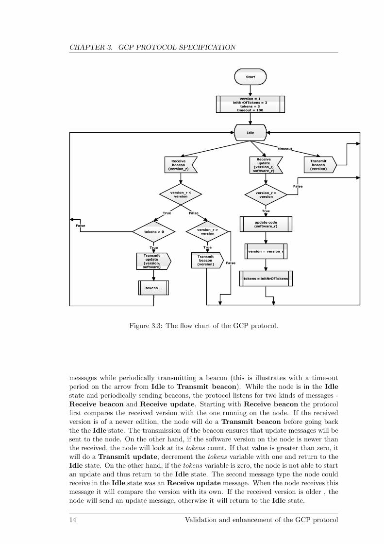
Figure 3.3 shows the flow chart of the GCP protocol. The GCP protocol startswith an initialization of the local variables version, initNrOfTokens, token and timeout.With the local variables initialized the protocol continues to the Idle state. This isthe main state of the protocol where the node listens for incoming beacons and update
Validation and enhancement of the GCP protocol 13
CHAPTER 3. GCP PROTOCOL SPECIFICATION
Start
version = 1initNrOfTokens = 3
tokens = 3timeout = 100
Idle
timeout
Receiveupdate
(version_r,software_r)
Transmitbeacon(version)
Receivebeacon
(version_r)
version_r <version
True False
version_r >version
tokens > 0
True
Transmitbeacon(version)
True
Transmitupdate(version,software)
False
False
True
tokens = initNrOfTokens
version = version_r
update code(software_r)
version_r >version
False
Figure 3.3: The flow chart of the GCP protocol.
messages while periodically transmitting a beacon (this is illustrates with a time-outperiod on the arrow from Idle to Transmit beacon). While the node is in the Idlestate and periodically sending beacons, the protocol listens for two kinds of messages -Receive beacon and Receive update. Starting with Receive beacon the protocolfirst compares the received version with the one running on the node. If the receivedversion is of a newer edition, the node will do a Transmit beacon before going backthe the Idle state. The transmission of the beacon ensures that update messages will besent to the node. On the other hand, if the software version on the node is newer thanthe received, the node will look at its tokens count. If that value is greater than zero, itwill do a Transmit update, decrement the tokens variable with one and return to theIdle state. On the other hand, if the tokens variable is zero, the node is not able to startan update and thus return to the Idle state. The second message type the node couldreceive in the Idle state was an Receive update message. When the node receives thismessage it will compare the version with its own. If the received version is older , thenode will send an update message, otherwise it will return to the Idle state.
14 Validation and enhancement of the GCP protocol

3.1. GCP PROTOCOL
Reflection on the GCP protocol
From the construction of the flowchart different constraints of the GCP protocol becomesmore clear. Regarding the features of the radio no explicit assumptions are given in[9]. But unless the radio is full duplex situations will occur where the radio is busyreceiving/transmitting updates and thus cannot transmit the periodical beacon. Whichaction the authors takes in this situation is unclear. Another unclear situation is whathappens if a node crashes in the middle of a transmission/reception or while updatingthe running software. No explicit assumptions are found within [9]. The same appliesif the node should recover after a crash. Lastly, assuming no packet loss / collisionsin a wireless network is very limited and does not reflect the reality which makes thisprotocol less suitable for real implementation.
Summary
In this chapter we give a systematic specification of the GCP protocol. We start by defi-ning the service the protocol delivers. We then describe the different assumptions uponwhich the protocol is built. After this a vocabulary was specified and the message enco-ding was presented. Lastly, the procedure rules were created with help from flow charts.The last section contains a short discussion about different ambiguous specifications andcertain limitations in the protocol.
Validation and enhancement of the GCP protocol 15


Chapter 4
Verification of the GCP protocol
In this chapter we model the GCP protocol shown in Figure 3.3 as a timed automatonin UPPAAL. UPPAAL is a tool for modeling, validation and verification of real-timesystems modeled as networks of timed automata [23]. Using UPPAAL we verify that ourGCP model satisfy selected correctness properties. We ensure that the GCP protocolis free of deadlocks. We also verify the general update behavior of the GCP model,including correct tokens usage e.g the possibility of updating multiple nodes using onlyone token as specified in [9] We further extend the UPPAAL model with time, andenergy, allowing us to reason about best- and worst case code update propagation speedas well as energy consumption for selected topologies.
4.1 Initial GCP model
The initial model of a UPPAAL node process implementing the GCP protocol is illus-trated in Figure 4.1. The model reflects the mechanics of the GCP protocol modeled asa timed automaton, with no assumptions about the underlying hardware.
myRemoteVersion > version
myRemoteVersion < version
myRemoteVersion <= version
x >= timeout
tokens > 0
myRemoteVersion > version
tokens == 0
myRemoteVersion == version
beacon!
UPDATE_OWN
CHK_BEACON_V
CHK_UPD_V
x<100
x <= timeout
CHK_TOKENS
INIT
REQUEST_UPD
IDLE
update!
tokens := tokens − 1
remoteVersion := version
x:=0
x := 0,remoteVersion := version
myRemoteVersion := remoteVersion
myRemoteVersion := remoteVersion
version := remoteVersion,tokens := initNrOfTokens
update?
beacon?
beacon!
Figure 4.1: Initial GCP UPPAAL model
To explain the behavior of the initial GCP UPPAAL model we describe the individualstates of the model.
INIT - The node process starts in INIT state, here it will remain between 0 to 100time units, before it enters the IDLE state. We use the local clock x to keep trackof time. Having the invariant x < 100 in the initial state forces the process toleave the initial state after 100 time units. By delaying 0 to 100 time units fromthe initial state to the IDLE state, we model that nodes have randomly startingbeacon intervals.
Validation and enhancement of the GCP protocol 17

CHAPTER 4. VERIFICATION OF THE GCP PROTOCOL
IDLE In the IDLE state beacons will be broadcast periodically every 100 time units.We enforce this by having the invariant x ≤ timeout in the IDLE state, and byplacing the guard x ≥ timeout on the beacon! transition, where timeout = 100.We reset clock x when a beacon is broadcast from IDLE state. When broadcastingthe beacon! the node perform a one-way value passing of the update version thatthis node is currently holding. The version is passed to trough the shared variableremoteVersion
In the IDLE state it is possible to receive beacons and updates. The node can re-ceive a beacon by synchronizing upon the beacon? broadcast channel and receivean update by synchronizing upon the update? broadcast channel. The updateversion for both a beacon and an update is passed trough the shared variableremoteVersion and stored in the local variable myRemoteVersion upon synchroni-zation. When receiving a beacon the node will enter the CHK BEACON V state.When receiving an update the node will enter the CHK UPD V state.
CHK BEACON V The node check if the remote update is newer, older or the sameversion as the update the node is currently holding. If the remote version is newerthan the current version, the node proceeds to the REQUEST UPD state. If theremote version is the same as the current version the node returns to IDLE state.If the remote version is older than the current version the node will enter theCHK TOKENS state.
CHK TOKENS The node checks if it has enough tokens to broadcast an update. Ifthe node has more than zero tokens it will transmit the update update!, decreaseits number of tokens and enter IDLE state.
REQUEST UPD The node request a new update by broadcasting a beacon with thelocal update version.
CHK UPD V The node checks the version of the received update. If the version isolder or same as the current version we ignore it and enter the IDLE state. If the up-date version is newer than the current version the node enter the UPDATE OWNstate
UPD OWN The node stores the received update by assigning the remoteVersion tothe local variable version. The number of tokens are assigned to the initial tokenvalue.
The initial model introduced in 4.1 does not reflect the underlying hardware wethere for proceed to extend the model with some assumptions about the radio used forcommunication.
model assumptions
We assume that we use a half-duplex radio to send and receive messages, and assumethat the radio is always listening unless it is transmitting.
modeling
To model that we use a half-duplex radio, and that the radio is always listening unlessits transmitting we need to ensure that after the node process performs a transmits
18 Validation and enhancement of the GCP protocol

4.1. INITIAL GCP MODEL
operation, beacon! or update! the node process is able to receive incoming packets,beacons? or updates?.
The intermediate states CHK TOKENS and REQUEST UP are removed. Transi-tions originating from these two state are accessible from the CHK BEACON state. Thecheck of update version of the beacon is enforced by placing guards on the transitionsexiting the CHK BEACON state. To enable update reception after a transmitted bea-con, we add a transition from the CHK BEACON to the CHECK UPD V state thatsyncronize upon update?. The changes made to the initial model is illustrated in Figure4.2
version := myRemoteVersion,tokens := initNrOfTokens
x := 0,remoteVersion := version
myRemoteVersion := remoteVersion
myRemoteVersion := remoteVersionbeacon?
update!
update?
x < 100
beacon!
x <= timeout
update?
beacon!
myRemoteVersion > version
myRemoteVersion == version
myRemoteVersion <= version
x >= timeout
myRemoteVersion > version
tokens == 0 &&myRemoteVersion < version
myRemoteVersion > version
tokens > 0 &&myRemoteVersion < version
x:=0
CHECK_UPD_V
IDLE
UPDATE_OWN
CHK_BEACON_V
remoteVersion := version,tokens := tokens −1
myRemoteVersion := remoteVersion
remoteVersion := version,x := 0
INIT
Figure 4.2: Basic GCP UPPAAL model
Verification results
The first property of the initial GCP model we verify is a safety property ensuring thatthe GCP protocol is free of deadlocks. We setup a system of system of three nodeswith three tokens each. One of the nodes contain a new version of a code update. Weask the the UPPAAL verifier if a node will ever enter a state with no outgoing actiontransitions from the state itself, or any delayed successor states [23]. In UPPAAL thequery i formulated as the Query in 4.1 Will it hold invariantly that we will not reach astate that is deadlocked.
A[] not deadlock (4.1)
Another property we want to verify is that when ever we use a token, we are able toupdate at least one other node. Will it always hold that when N0 use a token, at leastone other node is updated.
A <> (N0.tokens == 2) imply (N1.version == 2 or N2.version == 2) (4.2)
Validation and enhancement of the GCP protocol 19

CHAPTER 4. VERIFICATION OF THE GCP PROTOCOL
Another property of the GCP protocol that we wish to verify is that we are able toperform updates of multiple nodes using only one token. We query the UPPAAL verifierif it there exist a trace where node N0 use only one token to update the two nodes N1and N2. As part of the query we ensure that N1 and N2 both got their update from N0by requiring that the token number of both N1 and N3 is at the initial token value 3.
E <> (N0.tokens == 2) imply (N1.version == 2 and N1.tokens == 3) and(N2.version == 2 and N2.tokens == 3)
(4.3)
The Query 4.1, 4.2 and 4.3 all pass verification, and we ensured that our system isdeadlock free, and performs updates according to specification.
4.2 Timing analysis
model assumptions
In our previous work [16] we treated three different components of a WSN software up-date scenario, that influence the code update propagation time and energy consumption,namely data optimization (DO), distribution protocol(DP) and execution environment(EE). We wish to examine the time and energy properties of the GCP protocol as a codeupdate distribution protocol. Before defining a time and energy model we first makeassumptions about both data optimization and the execution environment, as well asthe underlying hardware.
Data optimization
For the time and energy models we use no data optimization. This means that thetotal software update is sent as a binary, as performed by the Deluge update mechanism[16][7] It can be argued that using differential patching (delta patching) [16][19] for dataoptimization will minimize the code footprint for simple updates, hereby conservingenergy. As seen in [14] [19] the total amount of energy used applying a delta patch mayvary greatly. The amount of energy used to apply a delta patch is not linear to the size ofthe delta patch, but also highly depends on the binary layout of the executable update aswell as the memory type and structure on the target node [14]. The full binary update ischosen as it provides a more transparent code update footprint, to energy consumptionratio, when applying the patch at the target node.
Execution environment
For the models we assume that the EE is monolithic. Having a monolithic EE gives usefficient code execution that provides a strong correlation between the tasks involvedin the update and the actual MCU time spend while updating. This ratio is otherwisedistorted by the execution overhead of modular environments caused by the levels ofindirection, or hardware abstraction in the virtual machine EE.
Code update size
As a basis for the UPPAAL model we use the platform previously explored in [16], com-prising of the AT90CAN128 MCU [1] and the nRF24L01 radio [5]. In the AT90CAN128there is 128 kB of programmable flash memory available, structured in 512 pages of
20 Validation and enhancement of the GCP protocol

4.2. TIMING ANALYSIS
each 256 bytes. The flash memory space is divided into two sections, the boot loadersection and application program section. The size of the bootloader section can be de-fined to either 4, 8, 16 or 32 pages, trough the BOOTZS1 and BOOTZS2 register ofthe AT90CAN128 MCU [1]. We reserve 16 pages of flash memory for the boot loaderapplication, hereby leaving 496 pages of unused flash program memory. As we performtotal binary updates, using no external ram source, we need to reserve half of the flashprogram memory as a buffer for the update before it can be written to the applicationarea. The size of the buffer- and application area are both 248 pages allowing codeupdates of a maximum of 248 × 256 bytes = 62 kB. For the time and energy model wemake the worst case assumption that the size of all code updates are 62 kB [2]. Theflash memory layout is illustrated in Figure 4.3
Bootloader
Buffer
Application
0x0000
0xFFFF
0x7C00
0xF7FF
248 pages
248 pages
16 pages
16 bit
Figure 4.3: Flash memory layouthas
Update TX/RX time
We first calculate the time a node spends when transmitting or receiving an update.The radio is capable of transmitting 2 × 10⁶bps. We assume that we have no collisionsand no lost packages as in [9]. To send a 62 kB update, we also assume that the MCUtime reading data from memory is insignificant compared to the throughput of theradio, hence this will not influence the overall transmit time of the update. With theassumption that we have no collisions and no lost packages we calculate the time to senda 62 kB update in Equation 4.4.
TX Time =62 kB× 8 bit× 1024
2× 106 bits/s= 0.253952 ≈ 0.254 seconds (4.4)
With the aforementioned assumptions we can transfer a 62 kB update wirelessly in0.254 seconds.
The time spend sending and receiving an update is not the same. The receivingnode has additional processing to do by storing the update in buffer, and subsequentlymoving the update from buffer to the application area. In the follow we calculate thetime it takes to store an update in buffer. The flash memory of the AT90CAN128 isstructure in units of 256 byte pages [1]
Writing a single page in flash memory takes 4.5ms [1], to store a 62 kB update inbuffer we need to write 248 pages. We calculate the time it takes to store the update inthe buffer in Equation 4.5.
hasBufferWriteTime = 248 pages× 0.0045 seconds = 1.1160 seconds (4.5)
Validation and enhancement of the GCP protocol 21

CHAPTER 4. VERIFICATION OF THE GCP PROTOCOL
The receiving node use 1.116 seconds to store the update in buffer. As the receiver isnot able to store the data as fast as the transmitter can send it, the transmitting node isalso involved in the update for this period of time. Even though the transmitting nodeis involved in this period of time, the radio is not always fully active during the update.We use the 1.116 seconds as the time a transmitting node use to send an update. Asa basis for energy consumption we later use the 0.254 seconds as a rough estimate forthe active period the sending node is actually transmitting. We assume that the MCUis active during the entire update for both the sending and the receiving node.
When the receiving node has stored the update in the buffer, it needs to copy theupdate from the buffer to the application area. This write operation will consume anadditional 1.116 seconds and in addition to this we must add the time it takes to readthe 248 pages from the buffer.The read time of a full 256 byte page is not explicit in the AT90CAN128 data sheet, wetherefor derive an estimate on the total buffer read time, based on the AT90CAN128MCU architecture, the MCU frequency and a pseudo code example found in the AT90CAN128data sheet, dictating a ’byte by byte’ flash read operation.
The flash memory is read one byte at a time [3]. The pseudo code in Listings 4.1describes how to read first the low byte, then the high byte of a specific 16 bit flashaddress. This read operation consist of six instructions. As both high- and low bytesare stored in DATA register we add two move instructions, for at total of 8 instructionsas an estimate for the operations performed reading two bytes from the buffer.
1 Load Command 0x02 . // ReadFlash commandLoad Address High Byte (0 x00 0xFF ) .Load Address Low Byte (0 x00 0xFF ) .// Output Enable =0, B y t e S e l e c t 1 =0 ( Addr . word low b y t e now in DATA. )
5 Set !OE to 0 , and BS1 to 0// B y t e S e l e c t 1 = 1 ( Addr . word h igh b y t e now in DATA. )Set BS1 to 1Set !OE to 1 . // Output Enable = 1
Listing 4.1: Buffer read operation
The AT90CAN128 MCU is of Harvard architecture, this means, that the MCU uti-lizes a separate instruction- and data bus, allowing it fetch instruction, while executing.The AT90CAN128 MCU can hereby achieve speeds of up to 1 MIPS per MHz on opera-tions on the registers R0 - R31. Loads and store operations to and from memory use 1-2clock-cycles and branch operations use 1-4 clock cycles [1]. The AT90CAN128 is runningat 16MHz. All eight instructions use 2 clock cycles each [1][3], and we can calculate thetime to read a 248 pages of 256 bytes in Equation 4.6
BufferReadT ime =8× 2 cycles
16× 106 cycles/sec× 248 pages× 256 bytes
2 bytes= 0.031744 seconds
(4.6)
The total update time for the receiving node is calculated in Equation 4.7.
UpdateT imeReceiver = 2× 1.116 sec. + 0.031744 sec. = 2.2637 seconds (4.7)
22 Validation and enhancement of the GCP protocol

4.2. TIMING ANALYSIS
Modeling
For time analysis we extend the basis GCP UPPAAL model in Appendix B.2 with thenotion of transmission time, and connectivity. Using the extended GCP time analysismodel Appendix B.2 we wish to show the best- and worst case code propagation speedfor the synthetic topologies illustrated in Figure 4.4
(a) Straight line. (b) Center node. (c) Corner node.
Figure 4.4: Synthetic topologies
The synthetic topologies in 4.4 each reflect a specific placement of an updated nodein relational to a multiple number of non-updated nodes. Each topology will influencethe code update propagation speed as well as the use of tokens in its own way. UsingUPPAAL we reason about the best- and worst case code update propagations speed.
Connectivity
To do time analysis using the synthetic topologies in Figure 4.4 , we introduce the notionof connectivity to the GCP UPPAAL model.
We use a simple Beacon process illustrated in Figure 4.5 to explain how connectivityis modeled. The simple Beacon process can send and receive beacons. The Beaconprocess counts the number of sent and received beacons using the variables beaconsSentand beaconsRecv. The Beacon process will send a beacon every 100 time units.
link[id][remote_id]
!link[id][remote_id]
x<=100x >= 100
beacon?
beacon!
beaconsRecv++
var:=id,x:=0,beaconsSent++
remote_id:=var
Figure 4.5: Beacon process
When synchronizing on the beacon channel we perform a one-way value passing of thesending node id. The sending node passes its id to the receiving node trough the sharedvariable var. Synchronization at the receiving node will lead to a new intermediatecommitted state, from where we will decide if there is connectivity between the sendingan receiving node. The topology of the network is modeled as the adjacency matrix Linkin Table 4.1. To determine if the sending- and receiving nodes can communicate, thereceiving node perform a lookup in the Link matrix using its own id, and the id of thesending node, remote id. If Link[id][remoteId] = 1, the node identified by id receivesmessages sent by the node with remote id. The Link evaluation is placed as a guardupon the transition indicating that the nodes are connected, in this case incrementingthe number of beacons received, beaconCount. The negated Link evaluation is placed
Validation and enhancement of the GCP protocol 23

CHAPTER 4. VERIFICATION OF THE GCP PROTOCOL
as a guard on the transition leading back to the initial state hereby ignoring the effectsof the beacon synchronization as is if the two nodes were not connected. We test theconnectivity by verifying a UPPAAL system of two Beacon processes P0id=0 and P1id=1,using the connectivity array Link in Table 4.1 first in connected configuration, and nextin a non-connected configuration.
Connected Non-Connected
Link =
[0 11 0
]Link =
[0 00 0
]Table 4.1: Connected vs non-connected Link configuration
To verify that process P0 and P1 can communicate in the connected Link configu-ration we first query the UPPAAL verifier if it holds that when P0 sends a beacon, itwill imply that this beacon is received by P1.
E <> (P0.beaconsSent > 0) imply (P0.beaconsSent == P1.beaconsRecv) (4.8)
To ensure two way communication it must also hold that if P1 sends beacons, the numberbeacons sent by P1 must be equal to the number of beacons received by P0.
E <> (P1.beaconsSent > 0) imply (P1.beaconsSent == P0.beaconsRecv) (4.9)
To verify that process P0 and P1 can not communicate in the non-connected Linkconfiguration, we ask the UPPAAL verifier if it holds invariantly that the beaconsRecvtvariable of both P0 an P1 always will be zero, meaning that communication never occurs.
A[](P0.beaconRecv == 0) and (P1.beaconRecv == 0) (4.10)
All 3 queries pass verification, and we can apply connectivity as illustrated in Figure4.5 to the GCP model in Figure 4.6. ( A large scale Figure can be found in AppendixB.3)
Time
To reflect the passing of time in the model we introduce two new states SEND UPD andRECV UDP.
SEND UPD In this state the node will delay for the period of time it takes to send anupdate. The time it takes to send an update is stored in the constant SEND TIME.The invariant x ≤ SEND TIME in the SEND UPD state enforces the processto leave the state after SEND TIME time units. The guard x ≥ SEND TIMEplaced on the transition leading to the IDLE state enforces that the node cannottake this transition sooner than SEND TIME time units. The node processremains in the SEND UPD state exactly SEND TIME time units, and proceedsto the IDLE state.
RECV UDP In this state the node will delay for the period of time it takes to re-ceive an update. The time it takes to receive an update is stored in the constantRECV TIME. Using a combination of an invariant and a guard we ensure thatthe node remains in the RECV UPD state for the duration of RECV TIME timeunits, and then proceeds to the IDLE state.
24 Validation and enhancement of the GCP protocol

4.2. TIMING ANALYSIS
!link[remoteID][id]
IDLE
CHECK_UPD_V
link[remoteID][id]
link[remoteID][id]
!link[remoteID][id]
!link[remoteID][id]
x < 100
x <= timeout
x <= SEND_TIME
CHK_BEACON_V
INIT
RECV_UPD
SEND_UPD
x<=RECV_TIME
update?
beacon!
x >= timeout
myRemoteVersion <= version
update?
update!
beacon?
link[remoteID][id]
x >= SEND_TIME
myRemoteVersion > version
x >= RECV_TIME
myRemoteVersion > version
myRemoteVersion == version
tokens > 0 &&myRemoteVersion < version
tokens == 0 &&myRemoteVersion < version
beacon!
remoteID:=remoteNode,myRemoteVersion := remoteVersion
remoteVersion := version,remoteNode:= id,x := 0
x:=0
x:=0,version := myRemoteVersion,tokens := initNrOfTokens
x:=0
remoteVersion := version,remoteNode:= id,x := 0
remoteVersion := version,remoteNode:= id,tokens := tokens −1,x:=0
remoteID:=remoteNode,myRemoteVersion := remoteVersion
x:=0
remoteID:=remoteNode,myRemoteVersion := remoteVersion
x:=0
Figure 4.6: GCP UPPAAL time model
Verification results
Best-case code propagation speed
With connectivity and time as a part of the GCP UPPAAL model we can start to reasonabout the time characteristics of the GCP code propagation speed in the synthetictopologies in Figure 4.4 To retrieve the best-case code update propagation speed, wequery UPPAAL to generate the fastest trace where all nodes in the system are in anupdated state. We add the global clock g to the system as time keeper. When thefastest trace is found, clock g will yield the time duration for the best-case code updatepropagation speed.
E <> N0.version == 2 and N1.version == 2 and N2.version == 2 andN3.version == 2 and N4.version == 2 and N5.version == 5
(4.11)
Worst-case code propagation speed
Determining the worst case code propagation time in UPPAAL and in general is notstraight forward task. We cannot ask UPPAAL for the for exact time for the worst casecode propagation speed, instead we manually narrow down this number by doing a binarysearch asking ”is it possible to have a non-updated system after a period timeBoundtime units”. Where we initially set timeBound to relatively high number and half thisnumber if the query fails. The binary search is illustrated in Figure 4.7
Final precision Start
TIME
Figure 4.7: Binary search for worst case code propagation speed
Validation and enhancement of the GCP protocol 25

CHAPTER 4. VERIFICATION OF THE GCP PROTOCOL
We formulate the initial query to obtain wost cast propagation speed in Query 4.12.
E <> not (N0.version == 2 and N1.version == 2 and N2.version == 2 andN3.version == 2and N4.version == 2) and g >timeBound
(4.12)If a query pass on a specific timebound it means that there are still non-updated
nodes within the timeBound, and we increase the time bound an query the UPPAALverifier again.
The time analysis result for best- and worst case code propagation speed is summa-rized in Table 4.2
Topology Best-case CPS Worst-case CPS
AStraigh Line 9.164 sec. ≈ 14.07 sec.
BCenter Node 2.416 sec. ≈ 10.26 sec.
CCorner Node 4.662 sec. ≈ 15.63 sec
Table 4.2: Best- and Worst case time analysis
As expected we see that best case code propagation is achieved in the center nodescenario, where all node can be updated using only one token. The slowest best-casepropagation is not surprisingly when all nodes are aligned, and each node must pass onthe update. The fastest worst-case propagation is the center node scenario, while theslowest being the corner node scenario.
4.3 Energy analysis
model assumptions
We calculate the energy consumed while sending and receiving updates, this includesenergy consumption by the transmitter/receiver as well as the MCU. We assume that theMCU is active while sending and receiving, and that the MCU is in idle state betweenthe periodical beacons.
We use the following typical power consumption characteristics for the nRF24L01and the AT90CAN128 in Table 4.3 and 4.3
Operational mode Supply current
RX (Low current mode) @ 3.3V 11.5 mA
TX @ 3.3V, -18 dBm 2000kpbs 7 mA
IDLE 22 µA
Table 4.3: nRF24L01 supply current
Operational mode Supply current
Active mode @ 25 ◦C, 4.5Vcc, 16MHz 27 mA
IDLE mode @ 25 ◦C, 4.5Vcc, 16MHz 16.5 mA
Table 4.4: AT90CAN128 supply current
We first use Equation 4.13 to calculate the energy consumption J . J is the quantityof energy in joules used for a given operation transmit,/receive of an update, and moving
26 Validation and enhancement of the GCP protocol

4.3. ENERGY ANALYSIS
update code from buffer. V is the supply voltage, I is the supply current. s is the timein seconds.
J = V ∗ I ∗ s (4.13)
The energy consumption of the nRF24L01 transmitting and receiving an update isdescribed in Equation 4.14 and 4.15 using the typical power characteristics in Table 4.3and the transmit time from Equation 4.4.
JnRF24L01 TX = 3.3V × 0.007A× 0.254s = 5.866× 10⁻³ ≈ 5.87mJ (4.14)
JnRF24L01 RX = 3.3V × 0.0115A× 0.254s = 9.637× 10⁻³ ≈ 9.64mJ (4.15)
The energy consumption of the AT90CAN128 while reading the buffer using thetypical power characteristics in Table 4.4 and the buffer read time as calculated inEquation 4.6
JReadBuffer = 4.5V × 0.027A× 0.031744 = 3.86mJ (4.16)
The energy consumption of the AT90CAN128 while writing an update to buffer usingthe typical power characteristics in Table 4.4 and the buffer write time as calculated inEquation 4.5.
JWriteBuffer = 4.5V ×0.027A×(248pages×0.0045s) = 0.13559400 = 135.59mJ (4.17)
Sender/Receiver Operations Energy
Energy SEND JnRF24L01 TX + JWriteBuffer 141.5 mJ
Energy RECV JnRF24L01 RX + 2× JWriteBuffer + JReadBuffer 284.8 mJ
Battery supply
We assume that a node is powered by three serially connected AA batteries. A singleAA battery characteristic is 1.5 volts, and 1100 maH. We assume that the voltage of thebattery is 1.5 volts during the entire discharge of the battery. We calculate the energyin three AA batteries in Equation 4.18
BatteryEnergy =1100 maH ∗ 3600 sec. ∗ 1.5 volts
1000× 3 batteries = 17820Joules
(4.18)Assuming that a node is continuously receiving updates performing no other actions, ais theoretically possible to receive 17820J×1000
248.8 mJ ≈ 62596 updates. This is highly optimistic
and will exceed the maximum of flash write/erase cycles. It should also be noted thatthe battery voltage eventually will drop below the operational voltage threshold for theAT90CAN128 during the discharge of the battery.
Validation and enhancement of the GCP protocol 27

CHAPTER 4. VERIFICATION OF THE GCP PROTOCOL
Modeling
To model energy consumption we introduce the meta variables energy and totalEnergy .In energy we accumulated the energy consumption of the individual node, in totalEnergywe accumulated the energy consumption of they entire system. When synchronizingupon the update! broadcast channel we add the energy consumption for a transmittedupdate to both the energy and totalEnergy variable. When receiving an update theenergy consumption for a received update is added to energy and totalEnergy.
To capture the time spend by a node in the IDLE state, we introduce a new processTicker, and add a looping transition in the IDLE state that synchronize on the tickbroadcast channel. The role of the Ticker process is to ”active” the node process inIDLE state. Ticker will broadcast a tick! each time unit, and allow we can herebyaccumulate the energy consumed in IDLE state When the node process synchronizeupon tick? we add the power consumed in one time unit (milisecond) to energy andtotalEnergy. The Ticker process is illustrated in Figure 4.8
t:=0t>=1
t <= 1
tick!
Figure 4.8: Ticker process
The energy extended GCP UPPAAL model is illustrated in Figure 4.9
remoteID:=remoteNode,myRemoteVersion := remoteVersion
remoteVersion := version,remoteNode:= id,x := 0
x:=0
x:=0,version := myRemoteVersion,tokens := initNrOfTokens,energy += RECV_ENERGY,totalEnergy += RECV_ENERGY
remoteID:=remoteNode,myRemoteVersion := remoteVersion
remoteVersion := version,remoteNode:= id,tokens := tokens −1, energy+=SEND_ENERGY,totalEnergy+=SEND_ENERGY, x:=0
remoteID:=remoteNode,myRemoteVersion := remoteVersion
x:=0
remoteVersion := version,remoteNode:= id,x := 0
INIT
CHK_BEACON_V
SEND_UPD
x:=0
x:=0
CHECK_UPD_V
idleTime++,energy+=IDLE_ENERGY,totalEnergy+=IDLE_ENERGY
IDLE
RECV_UPD
myRemoteVersion > version
myRemoteVersion <= version
myRemoteVersion == version
tokens == 0 &&myRemoteVersion < version
x < 100
x >= timeout
x <= SEND_TIME
x<=RECV_TIME
!link[remoteID][id]
link[remoteID][id]
!link[remoteID][id]
!link[remoteID][id]
link[remoteID][id]
tokens > 0 &&myRemoteVersion < version
myRemoteVersion > version
link[remoteID][id]
x >= SEND_TIME
x >= RECV_TIME
x <= timeoutbeacon?
update!
update?
beacon!
tick?
beacon!
update?
Figure 4.9: GCP UPPAAL energy model
Verification results
Having the energy consumption reflected in the model we want to explore the worst caseenergy consumption within a given time bound.
28 Validation and enhancement of the GCP protocol

4.4. SUMMARY
We ask the UPPAAL verifier if there exist at trace where we have used more thana specified energy threshold, we denote EnergyLevel within a certain time bound thatwe denote TimeBound. We use clock g as a timer keeper for the global time, andtotalEnergy as the amount of energy consumed by entire system.
E <> (g < TimeBound) and (totalEnergy > EnergyLevel) (4.19)
If the Query in 4.19 is passed, we know that the system is able spend more energywithin the time bound, otherwise the system will always have energy within the timeframe. We want to find the highest value of EnergyLevel for which it holds that Query4.19 is satisfied. We perform a binary search to find the worst case energy consumptionbounded by the best- and worst-case code update propagation speed.
The task of searching the state space for the worst case energy consumption be-came extensively time consuming and we did not manage to produce comparable worstcase energy results for the chosen synthetic topologies, bounded by the best- and worstcase propagation speed. We acknowledge that UPPAAL CORA performs Cost Opti-mal Reachability Analysis and is the proper tool to use in search of worst case energyconsumption but we will have to leave this task for future work.
4.4 Summary
Through the verification chapter we presented simple mode to illustrate the mechanicsof the GCP model. We extend the initial UPPAAL GCP model in three stages, firstincorporating the assumption about the radio, and then time and energy use. We madeassumptions about the underlying hardware of the model, and calculated the time andenergy used during an update for both the sending and receiving node. We verified thatthe GCP protocol is free of deadlocks, and that the intended token uses is reflected inthe model. On the time extended GCP model we performed time analysis and find best-and worst case code propagation speed for three synthetic topologies. On the energyextended GCP model we performed energy analysis but were not able to generate results.
Validation and enhancement of the GCP protocol 29


Chapter 5
Simulation of GCP
This chapter introduces a discrete event simulator named Network Simulator 2 (NS2)[6][22]. In this tool we implement the GCP protocol and verify it behaves as we expect.Then the simulation scenarios are described so various tests can be conducted. Theresults will be compared with the original results presented in [9]. Finally, explanationsare given for the deviation and replications of the original results are created.
5.1 Introduction to NS2
The NS2 tool is a packet-level network simulator developed at DARPA VINT 1 as aproject collaboration between researchers at UC Berkeley, LBL, USC/ISI and XeroxPARC. It is a free open source tool which helps to simulate existing network protocols:TCP, UDP, routing, and multicast over both wired and wireless networks. The tool iswritten using to languages:
• C++ defines the internal mechanism, and is responsible for running the entiresimulation. Using this language we define the functionality of the protocol.
• Object-oriented Tool Command Line(OTCL) is used to set up the parametersfor the simulation. Such parameters could be defining the topology, configuringnetwork objects, and scheduling discrete events.
This separation makes the tool flexible, because in order to change the system para-meters, it is enough to change the simulation file. Hence it removes the necessity torecompile the entire code. Since the body of NS2 is fairly large, the compilation time isnot to be negligible.
Figure 5.1 shows how the NS2 tool works. Firstly, the OTCL interpreter processes ascript. Secondly, it creates objects that are linked to a shadowing objects in a compiledcode, adds events to the EventQueue, and runs the simulation. Thirdly, when thesimulation finishes, the results can be accessed using an OTCL interpreter and visualizedgraphically using the tool Network AniMator (NAM).
OTCL
script(simulation
case)ResultsOTCL Interpreter
NS library:
Event Scheduler
Network Component Objects
Agent/GCP
Figure 5.1: NS2 working principles
Event scheduler
The NS2 performs centric discrete event simulations. Discrete event simulation organizesevents in chronological order in a fitting data structure referred to as the EventQueue.
1Defense Advanced Research Projects Agency Virtual InterNet Testbed
Validation and enhancement of the GCP protocol 31

CHAPTER 5. SIMULATION OF GCP
Each event is described by the event time (when the event is handled), an unique id,a pointer to the next event, and the associated event handler object. Each event isprocessed one by one, and the associated ”handler” object deals with this particular typeof event, updating the state space of the simulation scenario accordingly to the queueand potentially spawns one or more events. These events are subsequently inserted intothe EventQueue ordered by the event time before the next event is processed. When anevent has been processed, the global clock ”jumps” to the time stamp of the next eventin the EventQueue, and the next event is processed.
An example is illustrated in Figure 5.2 with two nodes A and B. We assume thenodes are within communication range, and with no packet loss will not occur.
1. The earliest event from the EventQueue is node A sending a beacon packet to itsneighbourhood. The event is handled by a network object, in this case sensor nodeA.
2. The handler for node A, will in turn call other networks objects affected by thisparticular event, in this case Node B.
3. When Node B has been made aware that it has received a beacon, it will generatea new event. The event generated will broadcast an update packet, assuming thatthe beacon version sent from Node A, is older that the version of Node B.
4. This new event is inserted into the EventQueue, and the next element of theEventQueue is processed.
EventQueue
time nextid handler
time next handlerid
handler()
handler()
insert
NetworkObject
NetworkObject
Node A
Node B
Figure 5.2: NS2 scheduling a beacon transmission from node A, and a replying updatemessage from node B.
Network component classes
Basically, NS2 has two class hierarchies for both languages: a compiled hierarchy andinterpreted hierarchy. These classes can be either standalone or linked together usinga TCLCL interface. In Figure 5.3 we see a simplified C++ class hierarchy in NS2. Allinformation and graphically presented documentation for NS2 can be found at [4]. Tounderstand the class diagram of the NS2 tool in Figure 5.3 we first describe the labelsused:
• TCLObject. All classes deriving from this class forms a compiled hierarchy.
• Handler. Each event contains a handler which specifies the action and the dispat-ching event.
32 Validation and enhancement of the GCP protocol

5.1. INTRODUCTION TO NS2
• NSObject is a parent class for a network objects that are responsible for sending,receiving, creating, and destroying packet related objects.
• Classifier is responsible for forwarding the packet to several NSObjects. If, forinstance, a mobile node broadcasts a packet, then a classifier object forwards thispacket according to the headers to all nodes within range.
• Connector immediately forwards the received packet from one NSObject to anotherone.
• Application is a parent class of applications such as FTP, Telnet, Traffic Generatorand others.
• Agent is an endpoint where packets are constructed or consumed. It is used inimplementation of protocols, i.e, UDP, TCP, GCP, and others.
• Queue This class derives from the Connector class. The object of this class pro-cesses outgoing packets. It gives a representation of locations where packets may bekept or dropped. The process responsible for packets scheduling makes a decisionwhich packet should be serviced or dropped. There is also a buffer managementprocess that regulates the occupancy of a particular queue type. For instance,drop-tail(known as FIFO) or fair-queueing(FQ).
• The Packet class defines the type for all packets in the simulation and providesmember functions to handle any object by its type.
• Node itself is a stand-alone class. It can either act as a router to forward a packet,or as host to hand a packet to the agent attached to the specified port.
Connector
Application
Node
Agent Queue Packet
FTP Telnet ... TCP UDP GCP …Drop
TailFQ ...
Mobile
Node...
Packet
Headers
NSObject
Classifier
TCLObject Handler
«interface»
OTCL
«interface»
Default Action
Figure 5.3: A simplified C++ class diagram of NS2
Mobile networking in NS2
The Wireless model is an extension to the NS2 tool and was included by the CMUMonarch Project [17]. The extension provides new additional elements at the physical,link, and routing layers of the simulation environment. With this extension we can createan accurate simulation of either a wireless- or multihop ad hoc networks.
The mobile node may have one or more network interfaces attached to a channel.These channel carries packets between the mobile nodes. When a packet is put onto the
Validation and enhancement of the GCP protocol 33

CHAPTER 5. SIMULATION OF GCP
channel, it distributes a copy of the packet to all the network interfaces of that channel.The interfaces then use the radio propagation model [18] to make a decision of acceptingor dropping the packet. A basic schematic of a mobile node is shown in Figure 5.4. Inthe following we explain outgoing and incoming packets:
Outgoing Packets. When a packet arrives at the mobile node’s entry, it is passedand processed by a demultiplexer. If the destination IP address matches the mobilenode’s IP address then the packet is passed to the port demultiplexer, which handsthe packet to the respective destination agents. However, most packets will match thedefault target and be handed down to the routing protocol. It adds an IP address of thenext mobile node, which has to process the packet. The ARP table is used to resolvethe logical IP address with second layer physical address. For simplicity, IP addressesare reused at the MAC layer. The next step is to insert the packet into the interfacequeue(IFq). After this, the MAC object takes the packet from the top of IFq and sendsit to the networking interface(NetIF). Lastly, NetIF stamps the packet with attributessuch as the power and position of the transmitting interface and puts the copy of thepacket to the channel. The channel makes a copy to all other interfaces connected tothat channel.
Incoming Packets. A copy of each packet sent onto a channel is delivered to allnetwork interfaces at the time at which the first bit would be delivered at the real system.Each NetIF puts a mark on the packet with the receiving network interface attributesand invokes Radio Propagation Model(RPM) object. This object uses the transmittedand received stamps of network interface to calculate the power with which the packetis received. The NetIF uses the result to determine if it actually successfully receivedthe packet and hands the packet to MAC object. If the packet is error and collision free,it is passed to the mobile node’s entry point. At this point a decision is made whetherthe packet has to be routed to the next mobile node, or it has reached its destination.
5.2 Implementation of GCP
The core elements like protocols, packet level content and agent behaviour are imple-mented in C++. To test the GCP in NS2 we must implement GCP packet contentand a GCP Agent in C++ which defines the behaviour of the sensor node. We areusing the current release of NS 2.34. To begin we create a new directory ’gcp’ in theNS base directory in which we create the following two files that will make up GCPimplementation:
• gcp.cc which describes the behaviour of the entire protocol.
• gcp.h is a header file for gcp.cc file.
A class diagram of GCP protocol
In Figure 5.5 the class diagram of GCP is shown. It presents the objects that are usedby a GCP protocol. If the fields (methods or parameters) of the classes are empty, itmeans that we did not modify this class.
The following explains the the most interesting methods in the GCPAgent classthat are used directly for implementation of the GCP protocol. This class defines thebehaviour of GCP protocol. A description of the methods is given in the following:
• recv. It is used for getting, processing, and sending a packet out.
34 Validation and enhancement of the GCP protocol

5.2. IMPLEMENTATION OF GCP
LL
IFq
MAC
NetIF
RadioPropagationModel
Channel
Src/Sink
ARP
arptable_
uptarget_
uptarget_channel_
propagation_
uptarget_downtarget_
downtarget_
downtarget_
uptarget_
demuxport
entry_
demuxaddr
defaulttarget_RTagent
(DSDV)
255IP address
mac_
target_
Figure 5.4: Schematic layout of a mobile node [6]
Agent
+offset() : int
+access(in p : Packet) : hdr_gcp
+offset_ : int
+tag : control
+version : unsigned int
+data : char
«struct»hdr_gcp
+command(in argc : int, in **argv : char) : int
+recv(in * : Packet, in * : Handler) : void
-isInRange(in dist : double) : bool
-getProbability(in r : float, in R : float, in dist : float) : float
-DecideIsInRange(in prob : float) : bool
-PMRand() : double
-paintGreen(in i : int) : void
-showResults(in i : int) : void
-OutputToFile() : void
+GCPAgent()
-token_ : unsigned int
-initNrOfToken_ : unsigned int
-version_ : unsigned int
-data_ : char
-tid_ : double
-noOfMessages_ : unsigned int
GCPAgent
+beacon = 0
+update = 1
«enumeration»
control
Packet
Handler
+getDistance(in i : int, in k : int) : float
God Schedular TCL
«struct»
hdr_ip
Figure 5.5: Class diagram of GCP protocol
• isInRange. Make a decision whether the packet will be forwarded for processingor discarded
• getProbability. Count the probability of getting the packet, when it is between3m and 5m
Validation and enhancement of the GCP protocol 35

CHAPTER 5. SIMULATION OF GCP
• DecideIsInRange. Check if the received packet is in a specified range.
• PMRand. Return a random number from 0 to 1.
• paintGreen. The method invokes TCL object and binds it with C++ in order tochange node colour at the time when node gets an update.
One of the most used methods is our receive method recv. This method describesthe main loop of the protocol.
The recv method
When a node receives a packet it unfolds it and takes the necessary data. In our case, weneed to access the headers of the ip and gcp protocols. After this, we count the distancebetween the sending and receiving nodes.
Every time a packet is received, the header is accessed, the distance is calculated andpassed on to the isitReachable method. If the node is within range we accept it, else itsdropped. If a packet is accepted, we check whether its a beacon or an update message.These two checks are described with code in the listing 5.1 and 5.2:
• A beacon received. The node compares the received version and its own. If thenode has an older version, it constructs a new packet of a beacon type and includethe version number where after the packet is transmitted.
recv ( Packet ∗pkt , Handler ∗). . .
i f ( hdr > v e r s i on > v e r s i o n )4 {
Packet : : f r e e ( pkt ) ; // f r e e memoryPacket∗ pkt re t = a l l o c p k t ( ) ; // a l l o c space f o r next packe t
8 hdr gcp ∗ hdrre t = hdr gcp : : a c c e s s ( pkt re t ) ;hdr ip ∗ i p r e t = hdr ip : : a c c e s s ( pkt re t ) ;
i p r e t > daddr ( ) = IP BROADCAST; //add broa dca s t add12 i p r e t > dport ( ) = ip r e t > spor t ( ) ; //add source por t
hdrret > tag = beacon ;hdrret > v e r s i on = v e r s i o n ;
16
send ( pktret , 0 ) ;}
. . .
Listing 5.1: Code example of receiving a newer version.
The code for receiving a lower version differs with few lines: the node adds anupdate tag instead of the beacon to the message together with the version number.After transmission, the token count is decremented.
• An update received. The node compares the received version and its own. If theversion is older than its own, it simply discards it. Otherwise, the node saves thetime stamp when it received the update, saves the update version, re-initializes itsnumber of tokens, invokes a paint function which adds the event to the EventQueue.Thus a node paints itself with a green colour(we use this for visualization), andoutputs the time and id to a file.
36 Validation and enhancement of the GCP protocol

5.2. IMPLEMENTATION OF GCP
1 i f ( hdr > tag == update ){
i f ( hdr > ve r s i on > v e r s i o n ){
5 t i d = CURRENT TIME;
v e r s i o n = hdr > v e r s i on ;// r e s e t tokens when we g e t update
9 token = initNrOfToken ;
paintGreen ( he r e . addr ) ;OutputToFile ( ) ;
13 }Packet : : f r e e ( pkt ) ;
}
Listing 5.2: Code example of receiving a new update.
A description of the simulation file
The code listed in listing 5.3 demonstrates the part of the protocol, where the nodessend a beacon message every 100ms. Firstly, we chose a node randomly which will getthe initial update. This node starts to send beacons after 1.000 seconds. After thetransmission the node saves the time so it knows when to transmit the next beacon.The other nodes start transmitting their beacons between 1.0 and 1.1 seconds and alsostore their sending time.
1 s e t randStart [ new RandomVariable/Uniform ]$randStart s e t min 1 .0$randStart s e t max 1 .1s e t l a s t v a l u e 0
5
s e t randNum [ expr { int ( ( $va l (nn) 1) ∗ rand ( ) ) } ] ;# choose random node$ns at 0 .0 "$p($randNum) set version_ 5" ;# a s s i g n newer v e r s i o n$ns at 0 .0 "$node_($randNum) color green" ;# i t becomes green
9 for { s e t i i 0} { $ i i < $va l (nn) } { i n c r i i } {
s e t startTime [ $randStart va lue ] ;# s t a r t i n g time between 1 .0 s;#and 1 .1 s for a l l nodes
13 for { s e t i 0} { $ i < [ expr $va l ( stop )∗1 0 ] } { i n c r i } {i f { $ i i == $randNum} {
i f { $ i == 0} {s e t startTime 1 .000 ;# s t a r t i n g time for f i r s t node
17 $ns at $startTime "$p($randNum) broadcast -beacon"
s e t l a s t v a l u e $startTime ;#save the l a s t time value} else {
s e t startTime [ expr $ l a s t v a l u e + 0 . 1 ]21 $ns at $startTime "$p($randNum) broadcast -beacon"
s e t l a s t v a l u e $startTime}
} else {25 i f { $ i == 0} {
$ns at $startTime "$p($ii) broadcast -beacon"
s e t l a s t v a l u e $startTime} else {
Validation and enhancement of the GCP protocol 37

CHAPTER 5. SIMULATION OF GCP
29 s e t startTime [ expr $ l a s t v a l u e + 0 . 1 ]$ns at $startTime "$p($ii) broadcast -beacon"
s e t l a s t v a l u e $startTime}
33 }}
}
Listing 5.3: Code example of the periodic transmission of beacons.
5.3 Basic GCP tests
To test that the GCP implementation works as expected, two simple test scenarios hasbeen devised.
The first test will demonstrate that the GCP implementation follows the procedurerules as described in Section 3.1. To avoid unpredicted behaviour caused by the non-uniform transmission probability described in 3.1, we set the transmission probabilityP = 1 for the purpose of this demonstration. In the demonstration illustrated in Figure5.6, six nodes are used A,B,C,D,E and F. Five nodes B,C,D,E and F have a fixed position.Node A will move from left to right along the x-axis, passing nodes B,C,D,E and F. Thereis no communication between any of the nodes B,C,D,E and F. With one exception, nodeA will not enter an area simultaneous covered by the transmission range of two or morenodes. The exception is when node A simultaneously passes node C and F. In the initialstate node B will have a new version of a code update. Nodes with the new code updateare indicated with the blue colour. The maximum number of update tokens is 2. Forthe experiment we initially set n = 0. The initial number of update tokens for node B,is assumed to be greater than zero, tokensB > 0. The initial number of tokens for thenodes C,D,E and F can be arbitrary in the interval 0 ≤ tokensC,D,E,F ≤ 2 as it will notinfluence the experiment, hence omitted in the illustration Figure 5.6.
A
B C D E
n = 0
x axis
y axis
F
(a) Test initial state
A
B C D E
n = 0
x axis
F(free)
n = 2 n = 1 n = 0
y axis
(b) Expected test behavior
Figure 5.6: GCP implementation test scenario, where node B contains a newer version.
Node A will move past node B, hereby receiving an update, and setting the numberof tokens n = 2. Node A moves past node C and F, updating both these nodes, spendingonly one token n = 1, this shows that one of the nodes C or F is receiving a ”free” update.As node A moves further right node D is updated, again using one token, n = 0. Asnode A reaches node E, node A is unable to perform further updates as n = 0, and nodeE will not be updated.
The second test will show that the transmission probability described in Section 3.1is reflected in the simulation. Five nodes B,C,D,E and F are placed with increasingdistance to node A, illustrated in Figure 5.7. Node A will transmit 10000 packets.
38 Validation and enhancement of the GCP protocol

5.4. SIMULATION SCENARIOS
We will count the number of packets received at node B,C,D,E and F respectively andexamine how the number of received packets corresponds to the transmission probabilitydescribed in Section 3.1, test results are shown below in Table 5.1.
A B C D E F
Figure 5.7: GCP range test setup
Node Distance d Received packets Sim. P (d) Calc. P (d) Deviation
B 3.0m 100000 1 1 0
C 4.0m 85836 0.85836 0.856847 0.0015134
D 4.5m 71581 0.71581 0.715625 0.0001850
E 5.0m 30151 0.30151 0.3 0.0015100
F 5.5m 0 0 0 0
Table 5.1: GCP range test result
Test results show that the simulated transmission probability Sim.P (d) and thecalculated transmission probability Calc.P (d) are closely matched, and P (d) only differswith a maximum of 0.001534 with 10000 packets send.
With the implementation behaving as expected we continue with a description of thedifferent test scenarios.
5.4 Simulation scenarios
In [9] the test scenarios are divided into two groups, synthetic and realistic. The sectionsdescribing the movement of synthetic- and realistic nodes in gives rise to confusion.Parameters for random movement is given in the realistic simulation section along witha dataset of realistic movement of 100 individuals, captured at MIT campus in theacademic year 2004-2005. This makes no sense because the movement of the peopleinvolved with the realistic test is recorded in the dataset. Also, no explicit assumptionsregarding movement is given in the synthetic simulation. Therefore we assume, that therandom movement parameters is misplaced within [9] as the realistic simulation scenariodraws upon the movement patterns captured in the fore mentioned dataset. This meansthat we use the parameters for random movement given in the realistic section in [9] todefine the movement of nodes for the synthetic simulation scenarios.
The movement parameters of the nodes given in [9] are somewhat ambiguous. Wepresent both our interpretations and compare the result with the results in [9] to selectthe most fitting.
One interpretation is, that every duration d, where 100ms < d < 500ms the nodechooses a random way point and moves towards it until a pause p comes and a newduration is commenced. The pause p is between 0ms < p < 100ms. If a new way
Validation and enhancement of the GCP protocol 39

CHAPTER 5. SIMULATION OF GCP
random way point is selected within each of these new durations, the overall result is anode moving around in a relatively small confined area. This setup will often result in anetwork that will remain fragmented throughout the entire simulation, as the movementof the nodes are insufficient to successfully spread the update. A fast analysis supportsthe simulation, because during 50 seconds of simulation and a maximum movementspeed of 2.0m/sec the maximum travel distance of a node is 2m/sec × 50sec = 100massumed the node always move in a straight line.
Having test scenarios in [9] that include deployment areas of sizes up to 2000m ×2000m the ”wandering” distance of the node is only a small fraction of this area, andwith frequent (100ms − 500ms) change of direction chosen by random, this movementapproach seams inadequate to distribute code updates to the sensor network in its en-tirety. An example of an early test simulation of 500 nodes in a 250m × 250m areaillustrating this problem (shown in Figure 5.8a). The graph shows that after 6 secondsof simulation approximately 440 nodes have received the update and the number doesnot grow in the following seconds. It should be noted that the updating process starts1 second after the initialisation, hence the number of nodes will first start to receiveupdates from the first second of simulation.
0
100
200
300
400
500
0 1 2 3 4 5 6 7 8 9
Num
ber
of N
odes
Time in seconds
Code propagation Speed - 1 cluster scenario
GCP - 3 tokens
(a) First interpretation.
0
100
200
300
400
500
0 1 2 3 4 5 6 7 8 9
Num
ber
of N
odes
Time in seconds
Code propagation Speed - 1 cluster scenario
GCP - 3 tokens
(b) Second interpretation.
Figure 5.8: Test results of two different interpretations of the random movement. Thex-axis shows the seconds of simulation and the y-axis shows the amount of nodes, whichhave received the update.
Another interpretation is to assign a new random way point only when the nodearrives at its current target way point. The duration is the same as described above, butinstead of having a movement pattern as a ”cloud” around the initial start point, themovement pattern changes to straight lines allowing the nodes to reach further around.A test simulation of 500 nodes in a 250m×250m using this movement model is shown inFigure 5.8b. The graph shows a continual growth in updated nodes and after 9 secondsof simulation, approximately 495 nodes have received the new update. It should benoted, that the same topology is used in both tests. If we solely look at the time framethe second interpretation is best since the overall number of updated nodes is higher,but also the characteristics of the graph is better. Comparing the two graphs, the first(a) shows an immediately updating process, but after a few seconds stops because therest of the nodes are too far away from the ”cloud” to receive an update. The othergraph (b) in Figure 5.8 shows a better curve. Within the first 3 seconds every node close
40 Validation and enhancement of the GCP protocol

5.4. SIMULATION SCENARIOS
to the source node gets updated. From there, the nodes move around and suddenlyafter the 4th second, one node reaches a new cluster thus the steep curve. From the 6thsecond, every node except nodes close to the borders has received the update. Finally,the progress slows down because the remaining nodes are scattered around the edge ofthe deployment area.
To conclude we choose the second interpretation because of the overall better achie-vements. Some of the additional information given regarding the different tests arecontrary if not ambiguous. In some of the cases the cluster sizes are not fully listed.In others, the amount of clusters and nodes are not specified. In order to clarify ourinterpretation of the different scenarios, we list them in the following two subsections.
Random waypoint movement
Each node is initially placed at a random location within the deployment area. At thestart of a simulation a node picks a random destination within the deployment area andmoves towards this destination with a speed randomly chosen between a predefined upperand lower bound, minSpeed , and maxSpeed. When a node reaches its destination itpauses for a period of time between a predefined upper and lower bound minPause, andmaxPause. The node alternately pause and then move to a new destination throughoutthe the entire simulation [13].
In the initial generation of movement patterns for the nodes we used the ’setdest’tool. Setdest is an independent tool for random movement generation bundled withthe NS2 distribution. The time to create random movement with ’setdest’ increasedexponentially with the number of nodes, and became very time consuming for clusterswith 2000 nodes or more. We found ’setdest’ to be slow, but also impractical to ourpurpose as the output from ’setdest’ required additional post-processing to reflect thecluster configuration of the individual simulation scenarios. We therefore wrote a smallpython application PyMove, that will generate random movement much faster(secondscompared to hours) while also reflecting the cluster configuration of a simulation scenario.PyMove generates a movement file that can be imported directly in NS2. An exampleof defining simulation scenario 3 through PyMove is listed in Listing 5.4.
1 from move import ∗
scene3 = Scene (50) // New scenery wi th 50 sec . s i m u l a t i o n time .scene3 . setSpeed ( 1 . 2 , 8 . 0 ) // min and max speed o f the nodes ( meter / s )
5 scene3 . setPause (0 , 100) // min and max pause o f the nodes (ms)// new C l u s t e r x , y , width , he i gh t , numberOfNodesscene3 . addCluster ( C lus te r ( 0 , 0 , 800 , 800 , 1000) )scene3 . addCluster ( C lus te r ( 700 , 700 , 800 , 800 , 1000) )
9 scene3 . generateMovement ( )
Listing 5.4: Defining simulation scene 3 through PyMove.
The cluster configuration generated by PyMove is visualized in Figure 5.9
It should be noted that the authors of [9] describe quote: ”Every movement is boun-ded by the defined area. The border rules are defined as each node bounce back accordingto the bisector of incidence angle”2. But there will never be any kind of bouncing, be-cause the random way point model will always chose a coordinate within the deploymentarea3. This means that a node can move to the border, but once it arrives it will choose
2[9] page 14 - middle of the page.3[13] page 11 - middle of the page.
Validation and enhancement of the GCP protocol 41

CHAPTER 5. SIMULATION OF GCP
Figure 5.9: Scenerio 3 visualized trough NAM.
a new random coordinate within the deployment area instead of bouncing as describedin [9].
Synthetic simulation scenarios
Each of the different synthetic scenarios will be run with the following random movementsettings:
(a) Scenario 4, two clusters (b) Scenario 5, four clusters (c) Scenario 6, four sociali-zing clusters
Figure 5.10: Examples of different cluster layouts.
• Nodes move according to a Random Way Point strategy for synthetic workload.
• Pause time: 0 - 100ms.
• Movement speed: 0.8 m/sec - 2 m/sec.
• Time is discretised by milliseconds.
• Beacon interval: 100ms
• Transmission range: r = 3 and R = 5, with a minimum transmission probabilityPmin = 0.3 inside range R.
• Simulation time: approx 50,000 ms.
42 Validation and enhancement of the GCP protocol

5.4. SIMULATION SCENARIOS
Synthetic scenarios:
• 1 cluster scenario. One large cluster composed of 2000 sensor nodes, in a 250m ×250m area.
• 1 sparse cluster scenario. One large cluster composed of 2000 sensor nodes, in a1100m × 1100m area.
• 2 cluster scenario. Two clusters of 1000 nodes, in two 800m × 800m areas, with asingle 100m × 100m intersection.
• 2 socializing cluster scenario. Two clusters of 950 nodes, in two 800m × 800mareas. The two clusters are put in a 2000m × 2000m area. The two clusters arenot within communication range. 100 additional nodes are inserted, and can movein the whole 2000m × 2000m area to ensure connectivity.
• 4 cluster scenario. Four separate 500 node clusters, in four 550m × 550m areas.Connectivity is ensured through a shared borders.
• 4 socializing cluster scenario. Four separated 475 node clusters in four 550m ×550m areas. The four clusters cannot communicate with each other. 100 additionalnodes are inserted, these nodes can move in the whole 1300m × 1300m area toensure connectivity.
• 9 cluster scenario. Nine separated 250 node clusters, in nine 400m × 400m areas.Connectivity ensured by a common borders.
• 9 socializing cluster scenario. Nine separated 240 node clusters, in nine 400m ×400m areas. The nine clusters are not within communication range of each other.90 additional nodes are inserted which move in the whole 1500m × 1500 area.
Realistic simulation scenario
For the purpose of testing GCP in a scenario with realistic movement behaviour theauthors of [9] use data sets that captures the location, communication, proximity andactivity information of 100 subjects at the Massachusetts Institute of Technology (MIT)over the course of the 2004-2005 academic year [9].
The simulation parameters presented below is identical to the parameters presentedin [9] with the except that we have moved information regarding the random movementto the synthetic test in Subsection 5.4.
• Time is discretised by milliseconds.
• Beacon interval: 100ms
• Transmission range: r = 3 and R = 5, with a minimum transmission probabilityPmin = 0.3 inside range R.
• Simulation time: approx 50,000 ms.
Validation and enhancement of the GCP protocol 43

CHAPTER 5. SIMULATION OF GCP
5.5 GCP test results
In this section we present the results of the GCP simulation. In each of the eightsynthetic test scenarios (described in Chapter 5.4) ten random topologies have beengenerated according to the parameters for the given test case. It should be noted thatin each simulation the node containing the update was randomly deployed.
Each of the ten generated topologies are used to run a test with 2,3 and 5 tokensrespectively. For all eight scenarios this gives the total amount of 240 data sets whichhave been used to generate two types of graphs (code propagation speed and load ba-lancing). All graphs are included on the appertaining CD. We emphasize the sourcenode is deployed randomly. This mean that even though the same topology is used toconduct a test with 2,3 and 5 tokens, the source node differs each time. Because of this,the code propagation speed between the different runs within the same topology cannotbe compared.
Scenario 1
In this scenario the size of the deployment area was 250 × 250 meters with 2000 nodes(dense). Looking at the graph for this test case with 2,3 and 5 tokens (displayed in Figure5.11 and 5.12 (a) - for bigger graphs, see Appendix C) we see two general features:
1. After the 50 seconds of simulation neither of the runs, disregarding initial tokencount, succeeds in updating all 2000 nodes.
2. After approximately 30 seconds of simulation the difference in code propagationamong the tests seems to be diminishing.
In the ten simulations with 2 tokens we managed to update between 1946 and 1974nodes which gives an average of 1961,5. With 3 tokens we managed to update between1955 and 1979 nodes with an average of 1972,1. In the simulation with 5 tokens weupdated between 1974 and 1987 nodes updated with an average of 1980,7. An illustrationof the averages can be seen in Figure 5.12b. Comparing the average amount of totalupdates in Figure 5.12 (b) we see the difference of the initial token count. In thebeginning of the simulation all nodes act alike since they have tokens left. The differencestarts to become more clear after 20 seconds of simulation. From this point the differencebetween having 2, 3 and 5 tokens is reflected in the update speed. Not surprisingly, thescenario with 5 tokens surpass the one with 3, which in turn surpass the one with 2.All graphs converge at the point where the problem changes from having tokens left toreaching the last nodes around the edges and corners of the deployment area. In ourcase the remaining nodes were never within range to receive the update.
For the same scenario the authors of [9] claim to update all 2000 nodes in 1,7 seconds4.Our results do not support this claim. Within 2 seconds we achieve to update less than100 nodes on average. It should be noted that the shape of our graph resembles thatof [9], so a possible error could be a wrong display of time in their figure. We alsonote, that some of their graphs looks strange. An example is the graph from scenario6, where the network consist of 4 separated clusters. In this scenario transmitters musttravel 200 meters to relay an update from one cluster to another. This should resultin a staircase shaped graph, but their graph is smooth. Because the source node wasdeployed randomly, the possibility arises where the source node was placed in a corner
4Code Propagation Speed - 1 dense cluster scenario. 1 Figure in the appendix of [9]
44 Validation and enhancement of the GCP protocol

5.5. GCP TEST RESULTS
0
500
1000
1500
2000
0 10 20 30 40 50
Num
ber
of N
odes
Time in seconds
GCP - Scenario 1 - Code Propagation Speed - 2 Tokens
N1N2N3N4N5N6N7N8N9
N10
(a) 2 tokens.
0
500
1000
1500
2000
0 10 20 30 40 50
Num
ber
of N
odes
Time in seconds
GCP - Scenario1 - Code Propagation Speed - 3 Tokens
N1N2N3N4N5N6N7N8N9
N10
(b) 3 tokens.
Figure 5.11: The x-axis displays the time in seconds, and on the y-axis display theamounts of updated nodes. (a) shows the result of ten runs of test scenario 1 with 2tokens. (b) shows the result of ten runs of the same scenario but with 3 tokens instead.
0
500
1000
1500
2000
0 10 20 30 40 50
Num
ber
of N
odes
Time in seconds
GCP - Scenario 1 - Code Propagation Speed - 5 tokens
N1N2N3N4N5N6N7N8N9
N10
(a) 5 tokens.
0
500
1000
1500
2000
0 10 20 30 40 50
Num
ber
of N
odes
Time in seconds
GCP - Scenario 1 - Average Code Propagation Speed - 2,3,5 Tokens
AVG 2 tokensAVG 3 tokensAVG 5 tokens
(b) Average.
Figure 5.12: The x-axis displays the time in seconds, and the y-axis display the amountsof updated nodes. (a) shows the result of ten test scenario 1 with 5 tokens. (b) showsthe average graph of 2,3 and 5 token.
of the deployment area. This could influence our results, but after an inspection of thevisualisation of each test we have confirmed that no such placement has happened.
Load balancing scenario 1 In order to estimate the load balancing, the numberof sent messages have been collected from each simulation. The results of scenario 1are illustrated in Figure 5.13. The graph shows the average token use throughout thesimulation. It should be noticed that our results resembles those from [9]. As expectedthe majority of the nodes used either 0 or 1 token. This is explained by the fact thata lot of the nodes reside close to the edge of the deployment area. When the updatereaches those nodes the rest of the deployment area has already been updated, thus notokens will be used.
It should be noted that the first updated nodes have a greater chance of using themost tokens, since every node they get into range of will need the update. This becomesmore clear when the initial token count is increased. Another important factor is the
Validation and enhancement of the GCP protocol 45

CHAPTER 5. SIMULATION OF GCP
random movement speed of the individual nodes. Among the firstly update nodes, someof them will choose a fast movement speed and a way point close to the edge of the area.Because of this, they have a chance to move faster than the spreading cloud of updatingnodes and thus encounter nodes who will request the update. If such an event happensthe node will possibly use all available tokens. As the graph shows though, this is rarelythe case. For instance, the number of nodes using 5 tokens is only 11,4 in average.
0
200
400
600
800
1000
1200
2 Tokens 3 Tokens 5 Tokens
Nu
mb
er
of
no
de
s
Number of used tokens
GCP - Scenario 1 - Load Balance - 2,3,5 Tokens
0 tokens1 tokens2 tokens3 tokens4 tokens5 tokens
Figure 5.13: On the x-axis the number of tokens is displayed and on the y-axis thenumber of nodes are displayed. The graph shows the average amounts of used tokens inscenario 1. It should be noted that nodes which did not receive any updates would nothave anything to transmit and thus would not use tokens. Therefore, the first pillar with0 tokens contains the combined amount of nodes which did not transmit any update ordid not receive any.
Scenario 2 - 8
The reflection upon the simulation results from scenario 2 to 8 has been gathered intothe same subsection because the results are similar. Common for each of these scenariosare the size of the deployment area is huge compared with scenario 1, but the numberof nodes stay the same. This gives a lower average density and thus a problem arisesbecause the distance between nodes become too large. This means that the source nodewill have to spend a lot of simulation time moving into range on another node, thus onlya few notes will get updated.
We choose to show the results for scenario 2 because it has the lowest average distanceof the seven scenarios given uniform distribution and thus should provide the best results(in theory, though in practice they are almost identical).
The results from scenario 2 is depicted in Figure 5.14 and 5.15(large pictures can befound in Appendix C). Every run shows the same low performance and the characteristicis apparent in the graphs for the rest of the scenarios. In 50 seconds of simulation thenumber of nodes which get updated are between 0 and 11. It should be noted that someof the runs did not succeed in updating any nodes and thus has been omitted from thegraph. This is extremely low, especially compared with the result of [9] which updateall 2000 nodes in less than 20 seconds of simulation time 5.
5Code Propagation Speed - 1 sparse cluster scenario. 2 Figure in the appendix of [9]
46 Validation and enhancement of the GCP protocol

5.5. GCP TEST RESULTS
0
2
4
6
8
10
12
14
0 10 20 30 40 50
Num
ber
of N
odes
Time in seconds
GCP - Scenario 2 - Code Propagation Speed - 2 Tokens
N1N2N3N4N5N6
N10
(a) 2 tokens.
0
2
4
6
8
10
12
14
0 10 20 30 40 50
Num
ber
of N
odes
Time in seconds
GCP - Scenario2 - Code Propagation Speed - 3 Tokens
N2N3N4N6N7N8N9
N10
(b) 3 tokens.
Figure 5.14: The x-axis displays the time in seconds, and on the y-axis display theamounts of updated nodes. (a) shows the amount of nodes in scenario 2 updated withan initial token count of 2. It should be noted that the figure does not contain tengraphs. This is because run N7,N8 and N9 did not succeeded in updating any nodesand thus was omitted. (b) shows the same scenario but with a token count of 3. Again2 runs - N1 and N5 - did not succeed in updating any nodes and was omitted. Commonfor both Figures are their low performance.
0
2
4
6
8
10
12
14
0 10 20 30 40 50
Num
ber
of N
odes
Time in seconds
GCP - Scenario 2 - Code Propagation Speed - 5 tokens
N2N3N4N5N6N8
Figure 5.15: The x-axis displays the time in seconds, and on the y-axis display theamounts of updated nodes. This figure shows the number of nodes updated with atoken count of 5. Like in the test with 2 and 5 tokens some of the ten runs did notsucceed in updating any nodes. Therefore, N1, N7, N9 and N10 has not been shown inthe graph.
Again, we find the result in [9] very doubtful. To update every node within the 50seconds simulation time is impressive, but with these distances between each node andthe short radio range and the slow movement it becomes unlikely in our opinion.
Load balancing scenario 2 Because of the low performance in the scenario 2 graphsfor load balancing has not been made. The same applies for scenario 3 to 8. They alllook the same. None of the 2000 nodes have received the update and thus used zerotokens except a few nodes who was very close to source node.
Validation and enhancement of the GCP protocol 47
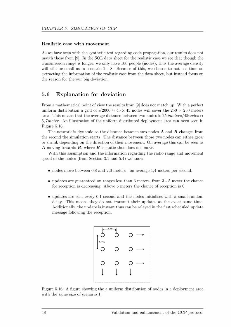
CHAPTER 5. SIMULATION OF GCP
Realistic case with movement
As we have seen with the synthetic test regarding code propagation, our results does notmatch those from [9]. In the SQL data sheet for the realistic case we see that though thetransmission range is longer, we only have 100 people (nodes), thus the average densitywill still be small as in scenario 2 - 8. Because of this, we choose to not use time onextracting the information of the realistic case from the data sheet, but instead focus onthe reason for the our big deviation.
5.6 Explanation for deviation
From a mathematical point of view the results from [9] does not match up. With a perfectuniform distribution a grid of
√2000 ≈ 45 × 45 nodes will cover the 250 × 250 meters
area. This means that the average distance between two nodes is 250meters/45nodes ≈5, 7meter. An illustration of the uniform distributed deployment area can been seen inFigure 5.16.
The network is dynamic so the distance between two nodes A and B changes fromthe second the simulation starts. The distance between those two nodes can either growor shrink depending on the direction of their movement. On average this can be seen asA moving towards B , where B is static thus does not move.
With this assumption and the information regarding the radio range and movementspeed of the nodes (from Section 3.1 and 5.4) we know:
• nodes move between 0,8 and 2,0 meters - on average 1,4 meters per second.
• updates are guaranteed on ranges less than 3 meters, from 3 - 5 meter the chancefor reception is decreasing. Above 5 meters the chance of reception is 0.
• updates are sent every 0,1 second and the nodes initialises with a small randomdelay. This means they do not transmit their updates at the exact same time.Additionally, the update is instant thus can be relayed in the first scheduled updatemessage following the reception.
5.7m
5.7m
Figure 5.16: A figure showing the a uniform distribution of nodes in a deployment areawith the same size of scenario 1.
48 Validation and enhancement of the GCP protocol

5.6. EXPLANATION FOR DEVIATION
Best case scenario 1
We now try to estimate the best case scenario for the results presented in [9]. In 1,7seconds the nodes can move 2 meters at best since movement would take 1 second. Thismeans that every node has to be in range of at least another node and the entire networkis somehow connected after the first second when the update process starts. In the bestcase every radio transmission will be received up to 5 meters away. Assuming thatthe source node is dropped directly in the middle of the deployment area and instantlyupdates as soon as possible, nodes within 5 meters will receive the update. Now, afterthe first 1,0 second, initialisation has been made, the update get transmitted and thefirst wave of nodes receive it. They all have their first update message scheduled for1,01 and thus transmit the update. Now the next wave receives the update. Again -the nodes in the second wave have scheduled their update for 1,02 and thus transmitit. With an average count of 45 nodes per line in the node grid and the source nodeplaced in the middle, a total of 22 nodes has to be updated, thus 0,22 second is neededto update the nodes closest to the edges. From there, additional 0,22 is needed to reachthe nodes in the corners, which in total gives an update time of 1,44 seconds. So if thenodes are distributed so the range between is maximum 5 meters, the source node isdirectly in the middle and the scheduling of the individual nodes are perfectly alignedall 2000 nodes can receive the update in only 1,44 seconds.
A contradiction occurs since the gap between the nodes has to be 5,7 meter for auniform distribution. This could indicate that the authors of [9] either did not have auniform distributed topology or their radio had a longer range than described in theirwork.
Best case scenario 2
In scenario 2, the deployment area is 1100 × 1100 meters with 2000 nodes. If they areevenly distributed in that area the average range between two nodes will be:
1100√2000
≈ 24, 5meters
node
.
The distance between two nodes is 24,5 meters given an evenly distributed network.Calculating the average distances for scenarios 3 to 8, we even get somewhat largerdistances ranging from 24,6 to 25,3 meters. As said in the beginning of this subsectionthe results from scenario 2 to 8 are identical with small deviations.
To estimate the best case scenario, the assumptions about movement and radiorange mentioned above is used. This means that every message send can be receivedat a distance of 5 meters. The source node is dropped perfectly in the middle of thedeployment area so there is 550 meters to the edges of the area and 777,8 meters to thecorners. After 1 second of initialisation, the source node needs to travel 19,5 meters toa neighbouring node to get within radio distance. With 2 meters per second the sourcenode needs 10 seconds of simulation time to reach one neighbour and update it. Fromhere, the two source nodes can now within another 10 seconds update one other nodeeach, which gives a total of 3 updates in 20 seconds. This does not match the resultsshown in [9]. Again we must conclude that either some explicit assumptions has beenleft out, their time scale on their graphs are wrong, the topology is not uniform or theirradio settings does not match the assumptions given in their work.
Validation and enhancement of the GCP protocol 49

CHAPTER 5. SIMULATION OF GCP
5.7 Replicate results of GCP
In this section we change the settings of our movement and radio range in order to seewhat it takes to replicate some of the results in [9]. We wish to replicate is the codepropagation speed of scenario 1, scenario 2, scenario 5 and scenario 6. These scenarioshas been picked out because:
• scenario 1 and 2 are described in detail in the previous section
• scenario 5 and 6 are more complex scenarios than the first pair but easier thanscenario 7 and 8 (which requires extreme settings to match the original results).
To replicate the results we adjust the settings regarding radio range and movementspeed. It should be noted that they somewhat compliment each other in the way, thatincreasing the radio range could be seen as improving the movement speed as morenode will get visited and vice versa. It should also be noted that we only focus on codepropagation speed in the replication of the result of a given scenario.
Scenario 1
In less than two seconds the authors of [9] claim to update all 2000 nodes within a 250× 250 meter area (dense cluster). With the original settings of movement speed andradio range we managed to update in average 1961,5, 1971,2 and 1980,7 nodes(2,3 and5 tokens respectively) in 50 seconds. This means that the goal is twofold:
• lower the update time to a maximum of 2 seconds.
• update close to 2000 nodes.
We incrementally increased the movement speed and radio radio range while com-paring the new result with those in [9]. With a movement speed of 15 to 20 meters persecond and a radio range of 6 - 10 meters we managed to update 1999 nodes in 1,38seconds. These settings are far higher than those given in the GCP report. To replicatethe results from scenario 1 we had to increase the movement speed with a factor ten,and double the radio range. A picture of the graphs for the 10 runs with 3 tokens canbe seen in Figure 5.17a. A larger graph can be seen in Appendix D.
Scenario 2
Next we replicate the original results of scenario 2. This scenario is the sparse clusterwhere the authors of [9] claims to update all 2000 nodes in a maximum of 20 second.With the original settings we manage to update between 0 and 11 nodes in 50 secondsof simulation.
A possibility was the author somehow used the settings found in Subsection 5.7without knowing it. Therefore, we start by testing those settings in the replication ofscenario 2. These settings does not provide a result close to what the authors claim, soan increase of the settings are needed again. With a radio range of 17 - 23 meters persecond and a movement speed of 15 - 20 meters we managed to update all 2000 nodeswithin 20 seconds, which matches the results shown in [9]. Our results with 3 tokenscan be seen in Figure 5.17b. A larger graph can be seen in Appendix D.
As in the replication of scenario 1, the needed radio range and movement speedto replicate the results provided in [9] is far higher than stated. In this scenario themovement speed was a factor 10 higher and the radio was four and a half time longer.
50 Validation and enhancement of the GCP protocol

5.7. REPLICATE RESULTS OF GCP
0
500
1000
1500
2000
0 0.5 1 1.5 2
Nu
mb
er
of
No
de
s
Time in seconds
GCP - Scenario 1 - Code Propagation Speed - 3 Tokens (REPLICATED)
N1N2N3N4N5N6N7N8N9
N10
(a) Scenario 1: Ten runs with 3 tokens.
0
500
1000
1500
2000
0 5 10 15 20 25
Nu
mb
er
of
No
de
s
Time in seconds
GCP - Scenario 2 - Code Propagation Speed - 3 Tokens (REPLICATED)
N1N2N3N4N5N6N7N8N9
N10
(b) Scenario 2: Ten runs with 3 tokens.
Figure 5.17: The x-axis displays the time in seconds, and on the y-axis displays theamounts of updated nodes. (a) shows the amount of nodes in scenario 1 updated witha token count of 3, while (b) shows scenario 2. To create this replicated results themovement speed has been increased multiple times and so has the radio range, comparedto the original assumptions given in [9].
Scenario 5
This scenario contains four clusters aligned in a square. In this scenario the originalresults completes the update in less than 30 seconds. As before, we started with theprevious found settings but again had to increase the movement speed to increase thelikelihood that two nodes would go get close to a shared border, and the update couldbe transmitted from one cluster to the next. With a movement speed of 20 - 25 metersper second and a radio range of 17 - 23 meter we manage to update all four clusters in2 of the ten runs. This can be seen in Figure 5.18a - for larger figures see Appendix D.Each step on the graph is a new cluster which gets update. This means, that with thesesettings and 10 simulations we managed to update 4 clusters 2 times, 3 clusters 7 timesand 2 clusters 1 time.
We also discovered that increasing the radio range yields a better result when anupdate shall transmitted across a common border compared to increasing the movementspeed.
Scenario 6
The last scenario we are replicating contains four socializing clusters. This means thattransmitters will have to carry the update around and eventually enter the clusters whichwill lead to an update of it. The authors finish this update in less than 25 seconds. Withthe settings found in replication of scenario 5 we are not able to update more than 2clusters in 25 seconds of simulation, thus we increase the settings again. Our result canbe seen in Figure 5.18b. A larger graph can be seen in Appendix D. With a movementspeed of 25 - 30 meters per second and a radio range of 25 - 30 meters we managed toupdate all 4 clusters in four of the ten runs.
This indicates that with those settings an update of all 4 clusters is possible but stillwe need to further increase it if we want to update all clusters in each simulation.
Summarising the replication of the 4 different scenarios we see that the assumptionsabout the different settings provided in [9] does not produce the results presented in the
Validation and enhancement of the GCP protocol 51

CHAPTER 5. SIMULATION OF GCP
0
500
1000
1500
2000
0 5 10 15 20 25 30 35
Nu
mb
er
of
No
de
s
Time in seconds
GCP - Scenario 5 - Code Propagation Speed - 3 Tokens (Replicated)
N1N2N3N4N5N6N7N8N9
N10
(a) Scenario 5: 10 runs with 3 tokens.
0
500
1000
1500
2000
0 5 10 15 20 25
Nu
mb
er
of
No
de
s
Time in seconds
GCP - Scenario 6 - Code Propagation Speed - 3 Tokens (REPLICATED)
N1N2N3N4N5N6N7N8N9
N10
(b) Sceranio 6: 10 runs with 3 tokens.
Figure 5.18: The x-axis displayed the time in seconds, and on the y-axis display theamounts of updated nodes. (a) shows the amount of nodes in scenario 5 updated withan token count of 3, while (b) shows scenario 6, also 3 tokens. To create this replicatedresults the movement speed has been increased by multiple times together with the radiorange, compared to the original assumptions given in [9].
same article. Different events could be the reason of this. Firstly, the description of thescenarios were insufficient. Especially a change of topology or size of the deploymentarea would make a huge different. Secondly, they could have made a mistake whendefining the different settings of the movement speed and radio range. This is doubtfulthough, since no direct connection could be found in the increase of settings comparedto the scenarios.
5.8 Summary
In this chapter we have described the NS 2 tool in which we run our simulations. Wehave then described our implementation of the GCP protocol and afterwards verify thatit behaviour as we expect. To test this we have devised a few test cases. Then weintroduced the synthetic and realistic test cases which, in total, gives 9 different testscenarios. We run the 8 synthetic test cases and discovers the original results doesnot match ours. Our results for scenario 2 to 8 resembles each other. In 50 secondsof simulation we only manage to update between 0 and 11 nodes. To investigate thiswe created best case scenarios and came to the conclusion, that the original resultspresented in [9] is very optimistic. Finally, we changed the original settings of the radioand movement speed to replicate the original results. We found out that the settingsshould be increased with multiple factors in order to produce a result that was somewhatsimilar with those presented in [9].
52 Validation and enhancement of the GCP protocol

Chapter 6
Extension of the GCP protocol
This chapter describes our extension of the GCP protocol. Firstly, we elaborate on themain problems with the original GCP protocol with focus on the lack of recovery ma-nagement. Hereafter, ideas to remove some of the problems within the original protocolwill be introduced and used to create the specification for our extension of the protocol.We call it eGCP. With these specifications we create an implementation and verified thatit behaved as expected. Finally, we compare the our extension with the GCP protocol.
6.1 Problems with the GCP protocol
In Chapter 3 we described the GCP protocol and noticed several problems:
• Transmitting beacons 10 times per second is expensive energy wise. Especiallywith a movement speed of 0,8 to 2 meters per second.
• One of the assumption mentioned in Section 3.1 was that collision and packet losseswas assumed not to occur.
• Another problem was the broadcast approach the GCP protocol used. Withoutthe assumption of nodes not crashing, broadcasting a beacon or update messagewill give rise to possible implosion. However, it is a rare event.
• Finally, some scenarios trigger multiple use of tokens instead of the intended one.If two sources are available to a node both will transmit their update and usea token. This problem contradicts the authors idea with evenly balanced codeupdate.
The GCP protocol described in [9] will give rise to implosion under certain conditions.An example could be a node enters the vicinity of a multiple number of nodes andbroadcasts a beacon with an outdated software version. Now, the entire neighbourhoodof that node will respond with update messages. The problem is illustrated in Figure6.1a and 6.1b, while the configuration of the WSN is listed in Table 6.1
Node Version Tokens
A 1 3
B 2 1
C 2 2
D 2 3
E 1 2
F 1 3
Table 6.1: WSN configuration.
Node A starts by broadcasting its beacon containing id and software version to theneighbouring nodes. The nodes B ,C ,D ,F receives the beacon broadcasted by node A.Since node F has the same software version as A, version = version r, no action willbe taken. On the other hand, nodes B ,C and D all have a newer software version thannode A, versionB ,C ,D > version r. Given that update tokens are available on nodeB ,C and D , tokensB ,C ,D > 0 these nodes will start to transmit their software versionto node A, hereby causing implosion while wasting tokens.
Validation and enhancement of the GCP protocol 53

CHAPTER 6. EXTENSION OF THE GCP PROTOCOL
A
B
C
D
E
F
(a) Node A sends beacon
A
B
C
D
E
F
(b) Node B,C,D sends update
Figure 6.1: Implosion problem in GCP
Specifying a recovery mechanism
In the GCP protocol a build-in recovery mechanism exists as long as the update can becontained in a single message. This means that if a node misses an update a new beaconwill be transmitted shortly after. Our recovery mechanism supports updates spanningover a multiple number of packets. To specify a recovery mechanism a lot of differentdecisions have to be made. We start from the top with specifying how a transmissionstarts and then proceeds to handling the different errors and packet losses.
In our protocol, the only communication that requires a recovery mechanism is ourupdate messages. When an update transmission is started, no handshake is used. Thenodes which need the update should be ready to receive it at all times so a handshakeshould not be necessary. Also, by keeping the amount of protocol messages at a minimumwe ensure that battery power is not used unnecessarily.
When the update has begun acknowledgement messages will not be transmitted backupon successful reception. Instead NACK-messages will be used in order to lower theamount of protocol messages needed. Another reason for using NACK-messages is thatit minimizes the chance that the source node will implode, compared to ACK-approachif the average number of neighbours is high.
The next part of the recovery/reliability mechanism is to ensure that in case of packetdrops or node crashes, the rest of the network can continue. We will start by defining therules of our recovery/reliability mechanism. It should be noted our recovery mechanismsomehow resembles the Go-Back-N instance of the Automatic Repeat-reQuest (APQ)protocol [21]. The difference is our implementation uses NACKs instead of ACKs, andthus the time-out responsibility is shifted from the original sender in Go-Back-N to thereceiver. Also, it should be noted that we cannot use the ”window” since it representsa queue of consecutive sequence un-ACKed packets.
Rules of recovery
• A beacon transmission will trigger a best update candidate election if a messagewith a higher version has come. number. The election picks the source node withthe highest version and token number (will be called the best candidate from now).The best candidate transmits its update.
• The candidate will continue to transmit the updates in numbered sequence startingwith the first packet continuing until the last packet has been transmitted.
• Whenever the update process starts, the receiving node starts a timer when thefirst packet is received. Each time the node receives the next packet in line or
54 Validation and enhancement of the GCP protocol

6.1. PROBLEMS WITH THE GCP PROTOCOL
one with a lower sequence number, the timer is reset. This will happen when thereceiving node looses and transmits a NACK-message. If the timer reach zero aNACK-message will immediately be broadcasted back to the source node. TheNACK-message contains the highest-in-sequence packet number received by thereceiving node. In order to do so, an node id is required of the source. We thereforadd a node id in the packet (detailed in subsection 6.1 ).
• If the receiving node detects a packet has been dropped, due to a jump in thesequence numbers, it will reply with a NACK-message containing the last packetnumber it received. Then the timer is restarted on the node who detected thepacket loss. If this timer reach zero before the node has received the lost packet thenode retransmit the previous NACK-message. This can continue until a thresholdof nack counts is reached, where the node will abort the update.
To grasp the rules mentioned above we explain them in a few different scenarios usingsequence diagrams.
Explaining our NACK-approach if node A (candidate node) is transmitting anupdate to node B , A will continue to transmit the packets until it either finish or receivesa NACK-message on a specific packet from B . When a NACK-message is received theprevious packet will be retransmitted and the candidate node continues from that packetnumber. This procedure can be seen in the sequence diagram in Figure 6.2.
:Node A :Node B
Transmit Beacon (v 1.3)
Transmit Update (2/3)
Transmit request_update
Transmit Update (1/3)
Transmit Update (3/3)
NACK Update (2/3)
Transmit Update (3/3)
Time out
Figure 6.2: A sequence diagram of the NACK-approach. The message containing the 3rdupdate package is lost. This leads to a time-out on the receiving node which generates aNACK-message containing the last received message which was the part second updatepackage. The source node A receives the NACK-message, retransmits the next packetindicated by nack and continues until all packages have been sent.
In the next sequence diagram in Figure 6.3 we see a case where an update packetis lost (it should be noted that the beacon transmission has been omitted). Node Bdetects the loss, transmit a NACK-message and starts the timer. Before the source nodeA receives the NACK-message it has already transmitted the next packet. This means
Validation and enhancement of the GCP protocol 55

CHAPTER 6. EXTENSION OF THE GCP PROTOCOL
that B will receive the next packet which will be dropped thus prevent a restart of thetime-out clock. This leads to another time-out on B which retransmit the previouslysend NACK-message and reset the timer. Before the third time-out, the second packetis received and the rest of the update goes as planned.
It should be noted the a buffer on the nodes could improve the performance. It isa waste to drop received packets just because they are not in sequence, but adding abuffer would put addition requirements on the target node. Additionally, the protocolwould need a control mechanism for the buffer which induce complexity. For future worka possibility could be to implement the ”sliding window” hinted in [20]. It should alsobe noted that our managing of the NACK-messages could be improved. By listeningfor packets from the source the node might receive a packet second in line and thustransmit a NACK immediate instead of waiting for the time-out. This will provide ahigher throughput, since throughput is not (typically) a prioritised resource this changewas moved to future work.
:A :B
Update 1/5
Update 2/5
Update 3/5 NACK 1/5
NACK 1/5Update 2/5
Update 2/5
Update 3/5
Update 4/5
Update 5/5
Timeout
Timeout
not Timeout
not Timeout
not Timeout
Figure 6.3: A sequence diagram of the NACK-approach where the initial election hasbeen omitted. The message containing the second update part is lost. This leads to atime-out which generates a NACK-message containing the last received message whichwas the first part of the update message. Before the source node A receives the NACK-message it transmit the third update message. The receiving node B now receives thethird message from A indicating that the NACK message was lost. Therefore, the time-out clock is not reset and shortly after, B retransmit the NACK-message and thenreceives the second message it was waiting for. The time-out timer is started againbut resets when the second update message is received again. The rest of the updatecontinues as normal.
We have identified a problem with our NACK-approach and the dynamic WSN. Themobile nodes will roam and if a node comes into range of a node while broadcasting anupdate, it will respond with a NACK, saying it missed the first update packages. Thiswill result in a restart of the entire update since the source node will retransmit the firstpackage and continue in sequential order. With a high node density, the probability forsuch an event is high. Just after deploying a node with a new update. The example is
56 Validation and enhancement of the GCP protocol

6.1. PROBLEMS WITH THE GCP PROTOCOL
illustrated in Figure 6.4.How severe the problem is depends on the average density of the scenario. Tests
will have to show if the precedent rules should be changed. A possible way to solve theproblem is to introduce some kind of packet number awareness. An example could be ifthe ratio between the packet number received divided with the total amount of packetsexceeds a predefined threshold the node should not transmit a NACK but instead dropthe update packets.
A
B
Figure 6.4: The node A is displayed broadcasting an update message together withits transmission range to it neighbouring nodes. Because of the moving nodes, node Bmoves through the area of A and thus might receive packets in the middle of the update.B will think the first messages was lost and thus broadcast a NACK-message back to Awhich will retransmit the entire update. Unfortunately, before the update is complete,B moves out of range of A thus the reset is a waste of time and energy.
Time-out Period
To select the proper value for the time-out variable is difficult. Its important to keep itas low as possible so NACK-messages can be transmitted as fast as possible. This way,the source node will react faster to the packet loss, thus speeds up the overall update.On the other hand, congestion can happen and sending more packets would be a badreaction compared to slowing down the transmission rate (induce longer time-outs). Apossible solution could be adding a randomly small delay to the time-out variable aftereach usage.
Saving tokens
The original idea using the tokens was, that every time a node transmitted an up-date, the token count decreases at the given node. This gives a better load balancing.Unfortunately, with the original design, possible implosion could happen under certaincircumstances. As mentioned in Section 6.1, if node A crashes and later wake up, itsneighbourhood might have received an update in the meantime. When A then transmitits beacon, ALL neighbours will start sending an update message back to it. This willresult in great collision but more importantly waste N−1 tokens, where N is the numberof nodes in the neighbourhood of A.
We propose to add additional information in the beacon and create a new messagetype. A byte is added to the beacon which contain the number of tokens left on the node.
Validation and enhancement of the GCP protocol 57

CHAPTER 6. EXTENSION OF THE GCP PROTOCOL
This way, each node has a way to announce through its beacon how many tokens it hasleft and thus indirect tell, how many times the node has transmitted update messagesof this version.
We create a new message type called request update. With this new message typewe change the way our nodes ask for updates. Previously requests for an update wasinitiated by a beacon-handshake. Instead, nodes will now transmit a beacon with itsversion number, node ID and available token count. When a node A receives a beaconwith a newer version than its own a election period of 100 milliseconds is started. Sincethe interval of beacons are 100 milliseconds, A will receive a beacon from each node inits neighbourhood within this election. The highest token count is stored together withits appertaining node ID. With this information, A will know which node within itsneighbourhood that has transmitted the least amount of updates and thus elects thatnode by sending a request update message (containing the ID of the node with the mosttokens left). This action will start the update process. If more nodes are tied with thehighest token count, the first one received within the election is chosen.
6.2 Specification of extension
In the previous section we presented some extensions to the GCP protocol to solve someof the issues regarding to the implosion and recovery mechanism. In this section, wereview our previous description of the GCP protocol from Chapter 3.1 and add our ownextension to it (abbreviated eGCP from now).
To describe our extension, the approach of [12] is used again:
Service
The service remain the same as in the original GCP protocol. Additionally, reliability isinsured for larger updates which span over multiple packets.
Environment assumptions
The assumptions are the same as in the original GCP protocol, with exception of colli-sions and data losses which are are possible now.
Message vocabulary
Two new message types, request update and NACK are added to the existing vocabularyof the GCP protocol. We have also changed the layout of the beacon packet shown inFigure 6.5 introducing nodes id and tokens fields. Moreover, we altered the updatepacket layout by adding extra fields such as nodes ID, packet number, total packetnumber. This is illustrated in Figure 6.6.
Message encoding
In order to implement our extension to the GCP protocol the original message encodingsare changed. Each node has an individual id, which is attached to the beacon messagetogether with its version number and token count. System now is susceptible to failures.The update message is changed, so it now contains the id together with the four values- the version number, the packet number, the total amounts of packets, and the datain the update. The reason for adding the id to the update message is, that roaming
58 Validation and enhancement of the GCP protocol

6.2. SPECIFICATION OF EXTENSION
nodes can receive an update in the middle of the process and thus transmit a NACK tothe right node. The request update message contains the id of the node with the mosttokens available. Lastly, the message NACK includes the id of the receiver together withthe last received packet number.
The information is outlined in the following listing:
beacon ( ID , vers ion , tokens )2 update ( ID , vers ion , pk nr , pk to ta l , data )
reques t update ( ID r )NACK(ID , l a s t r e c e i v e d )
The Figures 6.5, 6.6, 6.7, 6.8 illustrate the packet layout of the eGCP protocol.
versioncontrol
beacon packet
8 bit 8 bit
6 bytes
tokens
16 bit 16 bit
ID
Figure 6.5: eGCP beacon packet
versioncontrol data
update packet
8 bit 8 bit 0-25 bytes
32 bytes
pk_nr pk_total
16 bit 16 bit
ID
16 bit
Figure 6.6: eGCP update packet
control
request_update packet
8 bit
3 bytes
16 bit
ID_r
Figure 6.7: eGCP request update packet
Procedure rules
With the eGCP changes formally described the procedure rules can be addressed. Aswith the GCP protocol we use flow chart diagrams to describe the behaviour of theprotocol. First, we describe the different labels used in the flow charts. Thereafterwe address some special notation in the charts and finally present the diagrams with athorough explanation.
Validation and enhancement of the GCP protocol 59

CHAPTER 6. EXTENSION OF THE GCP PROTOCOL
control
NACK packet
8 bit
5 bytes
16 bit
ID last_received
16 bit
Figure 6.8: eGCP nack packet
It should be noted that the labels in the diagram still have the extension r, whichrepresents a variable from a remote node. Additionally, the labels ID, tokens and versioncan have the extension upd. These variables are containers for information regardingthe node with the newest version and highest amount of tokens - in other words the bestcandidate for transmitting the update.
• version represents the local version number of the software.
• ID is the unique identification number of the node.
• pk nr is the current packet number.
• pk total denoted the total amount of packets in a current update.
• tokens represents the current amount of tokens available on a sensor node.
• initNrOfTokens is the predefined number of tokens that initially are available ona sensor node.
• timeout is a function with take a parameter of time before an action is triggeredor must be taken.
• nack count is the amount of times a NACK message can be retransmitted.
• threshold is the maximum value for nack count.
• last received denotes the packed number a node last received successfully.
• software is the constructed image which is created after every packets in an updatehas been received.
After introduction of labels we continue with the description of the diagrams. Itshould be noted as in Section 3.1, states are marked with bold, message types inverbatim and variables with italic. Additionally, to keep the number of transitionarrows at a minimum we introduce duplicate states which are marked with a dottedline. For instance - every branch of the protocol returns to the main state Idle at somepoint so to minimise the use of long arrows, the state has been moved closer and shownwith a dotted edge. Lastly, in order to create the flow charts as clear as possible we havedivided them into separate pictures. To see where the previous chart ended and the newone begins we have used a double border to highlight this.
Starting with Figure 6.9 at the start, an initialization of the internal variables aremade and the protocol continues to the main state Idle. From here four different eventscan happen. Either the node can receive a beacon, receive a NACK, receive an update,receive an update request or transmit a beacon (if the token count is greater than zero).The following paragraphs address them individually in detail.
60 Validation and enhancement of the GCP protocol

6.2. SPECIFICATION OF EXTENSION
Start
Idle
version = 1initNrOfTokens = 3
tokens = 3timeout = 0ID_upd;
tokens_upd;version_upd;expected = 1last_received;pk_nr = 1pk_total;
threshold = 5;nack_count = 0;
Truetokens > 0timeoutTransmit beacon
(ID, version, tokens)Receive beacon
(ID_r, version_r, tokens_r)
False
Receive request_update(ID_r)
Receive update(ID_r, version_r, pk_nr_r,
pk_total_r)
Figure 6.9: The main part of the eGCP protocol.
Transmit beacon From the Idle state a predefined time-out occur and the nodechecks the token count. If the node has at least one token a beacon is transmitted andthe protocol returns to the Idle state.
Transmit update Figure 6.10 shows a detailed illustration of the ”Transmit update”process. Initially, the packet number is reset to one. This is done to ensure, thatthe updates are transmitted from the beginning. Now, the first update is transmittedincluding the version number, packet number, total amounts of packets, and data. Thenode waits for a short period for eventual NACK messages. If none was received itcompares the packet number with the total amounts of packets in the update. If thepacket number is less than the total, the packet number is incremented and the nextpacket is transmitted. If the packet number is equal with the total amount of packets inthe update, the node will conclude the update is finish, decrement its amount of tokensand return to the Idle state. If an NACK message is received, the node compares theid to ensure that the message was intended for it. If the id matches, the node changesthe packet number to the needed packet and continues transmitting updates until itreaches the total amount of packets in the update. If the id did not match the node justcontinues with transmitting the next update.
Receive beacon In the Idle state, the node can receive beacons. When a beacon isreceived, the node compares the versions. If the beacon contains a newer version, thenode will store the information in the local variables ID upd, tokens upd and version updas the best candidate. Now an election begins where the nodes listen for incomingbeacons. If it receives any, the node will compare the version number with the numberfrom its best candidate. If they are equal the node will look at their tokens. If the countis higher than the best candidate, the recent received beacon is stored. If the versionreceived is not equal but greater and token count is larger than 1, it is immediatelystored as the best candidate and the node returns to the Electing candidate state.From this state a node may receive a beacon or and update message. After a predefined
Validation and enhancement of the GCP protocol 61

CHAPTER 6. EXTENSION OF THE GCP PROTOCOL
Receive NACK(ID_r, last received)
Transmittingtimeout(10)
Transmit update(ID, version,
pk_nr, pk_total)
pk_nr <pk_total
timeout
True
pk_nr ++
ID == ID_r
True
pk_nr =last_received +1
Idle
False (pk_nr = pk_total)
tokens --
False
Figure 6.10: The transmission part of the eGCP protocol in detail.
period, a request_update is transmitted to the best candidate and the node returns tothe Idle state.
Receive update An illustration of the ”Receive update” process can be seen in Figure6.12. From the start, the node receives an update message and verifies that the packetnumber matches the expected value and the version is newer. If this is the case thepacket is stored, expected is incremented, the nack count is reset and the node returnto the Waiting for packet state. However, if the version is newer, but the packetnumber is lower than the expected, the nack count is reset and the node returns to theWaiting for packet state. If the version is lower or equal to the nodes own, it will justreturn to the Waiting for packet state. In the Waiting for packet state a time-outoccurs if the expected packet is not received within a predefined period. The node thenchecks its nack count and compare it with a threshold value. If the value is lower, a NACK
will be transmitted, the nack count incremented and the node returns to the Waitingfor packet state. If the nack count value reaches the threshold value and a time-outhappens, the update is discarded and the node returns to the Idle state. Finally, theexpected value will match the pk total r which indicate all packets has been received.The node then create the software image from the packets, update itself and return tothe Idle state.
Receive request update From the Idle state a node can receive a receive_update
message. When such a message is received and ID and token check is preformed. If itmessage was intended for the node and it has tokens left it will initialise its update andtransmit the update. However, if the receive_update message was not intended for thenode it returns to the Idle state.
6.3 Implementation of eGCP
As with the implementation of the GCP protocol we create a directory, which containsour eGCP source file and the appertaining header file. We have decided not to draw
62 Validation and enhancement of the GCP protocol

6.3. IMPLEMENTATION OF EGCP
True
version <version_r
ID_upd = ID_r;tokens_upd = tokens_r;version_upd = version_r;
Electingcandidate
Receive beacon(ID_r, version_r, tokens_r)
Receive beacon(ID_r, version_r, tokens_r
ID_upd = ID_r;version_upd = version_r;tokens_upd = tokens_r;
True
True
tokens_upd< tokens_r
version_upd==
version_r
timeoutTransmit
request_update(ID_upd)
Idle
False
False Idle
Falseversion_upd< version_r
False
Electingcandidate
True
True
Waiting forpackets
store packet;expected ++;
nack_count = 0;
version < version_r&&
expected ==pk_nr_r
Receive update(ID_r, version_r, pk_nr_r,
pk_total_r)False
Figure 6.11: The reception of a beacon in the eGCP protocol.
a class diagram of eGCP because it is similar to the diagram of GCP protocol. Thefollowing explains what we have added to the eGCP protocol.eGCPAgent. We have introduced 5 different timers that inherits from the abstractclass TimerHandler. These timers are responsible for controlling execution of the func-tions such as send update, send req, waiting nack timeout(), waiting req timeout(), andsend nack(). The name of the function explains its purpose. The following describestimers. However the timers need to be detailed:
• eGCPTimerWaitCNDT controls the time given to choose the best candidate.When the time expires the node sends a request message to the candidate node.
• eGCPTimerWaitNack represents the amount of time time for a nack message fromthe destination node.
• eGCPTimerWaitREQ defines the time a node waits for request messages fromother nodes. In this way the node that has an update will avoid implosion fromnodes that have chosen it as an update source at the same.
• eGCPTimerTriggerNack controls the time given to send out a nack message if thenode did not receive the expected message in the period of time.
Validation and enhancement of the GCP protocol 63

CHAPTER 6. EXTENSION OF THE GCP PROTOCOL
Waiting forpacket
version < version_r&&
expected ==pk_nr_r
Receive update(ID_r, version_r,
pk_nr_r,pk_total_r)
FalseTrue
store packet;expected ++;
nack_count = 0;version < version_r
&&expected > pk_nr_r
nack_count = 0; True
FalseWaiting forpacket
timeout FalseTransmitNACK
(ID, pk_nr)
nack_count==
threshold
nack_count ++;
True
Idle
Falseexpected ==pk_total_r
True
update node(software)
tokens = initNrOfTokens;
Figure 6.12: The reception of an update message in the eGCP protocol described indetail.
• eGCPTimerSendBCN defines the time given to send the beacon.
The send beacon method
In the OTCL simulation file we schedule the first beacon event. When the time comes,this event is dispatched and executed. This triggers the beacon send timer, which invokesthe sending procedure every 100ms if the node is not busy (for instance, sending anupdate). If the node is busy and has tokens left, it is rescheduled to send a beacon afterthe next 100ms. The following Listing 6.1 shows the implementation of the sendingprocedure.
// we have tokens and we are not busyi f ( tokens > 0 && al low send beacon ( ) == true ){
4 Packet ∗pkt = a l l o c p k t ( ) ; // c r e a t e packe thdr ip ∗ iph = hdr ip : : a c c e s s ( pkt ) ;hdr egcp ∗ egcph = hdr egcp : : a c c e s s ( pkt ) ;
8 iph > daddr ( ) = IP BROADCAST; // add i n f o to header
64 Validation and enhancement of the GCP protocol

6.3. IMPLEMENTATION OF EGCP
True
Transmit update(ID, version,
pk_nr, pk_total)
pk_nr = 1;pk_total = max_pk_nr;
ID == ID_r&&
tokens > 0
Receiverequest_update
(ID_r)Idle
False
Figure 6.13: The reception of a request update message in the eGCP protocol describedin detail.
iph > dport ( ) = iph > spor t ( ) ;
12 egcph > tag = beacon ; // a d d i t i o n a l i n f oegcph > v e r s i on = v e r s i o n ;egcph > tokens = tokens ;
16 send ( pkt , ( Handler ∗ ) 0 ) ; // send packe ttm send bcn . resched ( 0 . 1 ) ; // r e s c h e d u l e new beacon
}else i f ( tokens > 0)
20 tm send bcn . resched ( 0 . 1 ) ; // new sending time// i f we are busy
Listing 6.1: Send beacon procedure
The recv method
When a packet is handed to eGCP agent it is processed inside the recv method. Thefollowing describes what kind of actions have to be taken if the node receives a particulartype of a messageBeacon received. When the node receives a beacon, it checks if it is not busy. Ifthe timer is idle, the node saves the candidate and starts the timer for next possiblecandidates. When the next beacon arrives the node checks if it is a better candidate.When the time exceeds, the request message is sent to the best candidate. The followingpiece of code in Listing 6.2 demonstrates the procedure of choosing the best candidate.
i f ( accept beacon ( ) == f a l s e ) // busy{Packet : : f r e e ( pkt ) ; return ;}
3
i f ( tm wait cndt . s t a t u s ( ) == TIMER IDLE) // f i r s t cand ida te{
save cand idate ( hdrip , hdr , pkt ) ;7 tm wait cndt . re sched ( 0 . 1 1 ) ;
Validation and enhancement of the GCP protocol 65

CHAPTER 6. EXTENSION OF THE GCP PROTOCOL
return ;}
11 i f ( tm wait cndt . s t a t u s ( ) == TIMER PENDING) // o t her c a n d i d a t e s{
i f ( ver s ion upd == hdr > v e r s i on ) // v e r s i o n i s the samei f ( tokens upd < hdr > tokens ) // another has more tokens
15 save cand idate ( hdrip , hdr , pkt ) ;else {Packet : : f r e e ( pkt ) ; return ;}
else i f ( ver s ion upd < hdr > ve r s i on ) // another has newer v e r s i o nsave cand idate ( hdrip , hdr , pkt ) ;
19 else {Packet : : f r e e ( pkt ) ; return ;}}return ;
Listing 6.2: Save candidate procedure
Request received. When the node is chosen as a candidate it will receive a requestmessage form another node. However, it is possible that when the node starts informingother nodes that it has newer version, it will be the chosen by many nodes at the sametime, beacause the nodes will send request messages to that node. In order to avoidbroadcasting more update messages the node waits 40ms. Then it will start an updateprocess. The Listing 6.3 demonstrates how the request message is processed.
i f ( a c c ep t r eq ( ) == f a l s e ) // busy{Packet : : f r e e ( pkt ) ; return ;}
3 // message f o r mei f ( hdrip > daddr ( ) == here . addr && tokens > 0){
Packet : : f r e e ( pkt ) ;7 pkt nr = 1 ;
// wai t to r e c e i v e more messages// and then launch the update pr oces s
11 tm wait req . resched ( 0 . 0 4 ) ;}else Packet : : f r e e ( pkt ) ;return ;
Listing 6.3: A request received procedure
Nack received. When a nack message is received, the node checks if the addressmatches its own. The next step checks whether the message arrived on time. If yes, thenodes saves a last received packet number, that came within the nack message. Thenthe node resends this packet.
i f ( accept nack ( ) == f a l s e ) // busy2 {Packet : : f r e e ( pkt ) ; return ;}
i f ( hdrip > daddr ( ) == here . addr ) // packe t addressed f o r me{ // nack r e c e i v e d on time
6 i f ( tm wait nack . s t a t u s ( ) == TIMER PENDING){
pkt nr = hdr > pkt nr + 1 ; // l a s t r e c e i v e dPacket : : f r e e ( pkt ) ;
10 send update ( ) ;}
66 Validation and enhancement of the GCP protocol

6.3. IMPLEMENTATION OF EGCP
else {Packet : : f r e e ( pkt ) ; return ;}}
14 else {Packet : : f r e e ( pkt ) ; return ;}
Listing 6.4: A nack received procedure
Update received. The following piece of code in Listing 6.5 demonstrates theprocessing steps when a node receives an expected packet. When the update packetwith a right version is received , the node checks if it is necessary to stop the candidateelection timer that was started in the choosing candidate state. Next, the packet numberis compared with the expected. If yes, and it is the last packet, the node just resetsvariable values to the initial states, saves the whole update(changes the version). If it isnot the last packet, the node saves the packet and waits for another one by reschedulingthe sending nack timer.
i f ( hdr > pkt nr == 1)2 c a n c e l c a n d i d a t e t i m e r ( ) ;
i f ( hdr > pkt nr == expected ) // we got expec ted pk t{
6 pkt nr = hdr > pkt nr ;p k t t o t a l = hdr > p k t t o t a l ;
i f ( pkt nr == p k t t o t a l ) // l a s t pk t i s r e c e i v e d{
10 expected = 1 ; // r e s e tt imeout counte r = 0 ; // r e s e t
v e r s i o n = hdr > v e r s i on ; // save an update14 Packet : : f r e e ( pkt ) ;
tm t r i gge r nack . f o r c e c a n c e l ( ) ; // a l l p k t s are r e c e i v e d .} // Cancel t imerelse
18 {rm nodeID = hdrip > saddr ( ) ; // save the source node
rm nodePort = hdrip > spor t ( ) ; // id and por t in order// to know where to send nack
22 expected++;t imeout counte r = 0 ;tm tr i gge r nack . re sched ( 0 . 0 8 ) ; // wai t f o r another packe t
}26 Packet : : f r e e ( pkt ) ;
}
Listing 6.5: An update received procedure
The simulation file
In the process of implementing the eGCP protocol we found that our previous approachof defining beacon timer events, and timers in general trough the OTCL script is unprac-tical. Although we could capture the behavior of the GCP agent, problems arise whenmultiple timers are introduced in the eGCP protocol. In GCP we use a single timer andupdates are instant using only one packet. In eGCP there are states where we wait fora certain amount of time e.g. while electing the best candidate. A predefined beacontimer event trough OTCL would conflict with the behavior of the eGCP protocol, andpossible send a beacon in a state where a node is dedicated to listening. We therefor
Validation and enhancement of the GCP protocol 67

CHAPTER 6. EXTENSION OF THE GCP PROTOCOL
moved the handling of timers away from OTCL into the C++ implementation. TheeGCP protocol is hereby captured within the C++ implementation of the eGCP Agent.
Agent initialization. The following piece of code shows the eGCP agent initiali-zation. We set a number of tokens, packets, and attach the agent to the node.
1 for { s e t i 0} { $ i < $va l (nn)} { i n c r i } {s e t p( $ i ) [ new Agent/eGCP] # c r e a t e agent$p ( $ i ) s e t tokens $ in itToken # i n i t tokens$p ( $ i ) s e t p k t t o t a l 5 # s e t pkt no
5 $p ( $ i ) output name $ c p f i l e # s e t output f i l e$ns attach agent $node ( $ i ) $p ( $ i ) # attach agent}
Listing 6.6: Agent initialisation
Broadcast event scheduling. In the eGCP, as we see in Listing 6.7 we scheduleonly the first broadcast event in order to trigger the node to start sending the beacons.The following piece of code shows the scheduling process of the broadcast event.
1 for { s e t i i 0} { $ i i < $va l (nn) } { i n c r i i } { # a l l nodess e t startTime [ $randStart va lue ] # time 1 . 0 1 . 1i f { $ i i == $randNum} { # random node
s e t startTime 1 .000 # s t a r t s 1 . 05 $ns at $startTime "$p($randNum) broadcast -beacon" # add event
} else { $ns at $startTime "$p($ii) broadcast -beacon"}}
Listing 6.7: Start broadcasting process
6.4 Test of the extension
In order to test the eGCP protocol we devise different test scenarios. We conduct twodifferent tests in order to validate the implementation of eGCP.
eGCP test 1
The first test is designed to verify the selection of the correct candidate, and to check ifonly 1 token is used in the update process. To test this, we place 10 nodes within thetransmission range. Each of them has a unique token counts ranging from 1 to 10. Theten nodes are within reliable communication range. Then we place a node with a lowerversion in the same deployment area, which transmit a beacon. In the election periodeach of the candidates will send a beacon. Node A should choose the best candidateand request the update. The setup can be seen in Figure 6.14a.
GCP We expect node A to transmit the beacon. This will trigger an update fromevery node inside the deployment area and in total use 10 tokens.
eGCP We expect node A to initiate an election and choose the node with the highestamount of tokens. Each node deployed has a unique token number ranging from 1 to10. This means that A should request the update from the node who has the 10 tokensavailable. After the simulation we expect to have node A updated with only 1 tokenused.
68 Validation and enhancement of the GCP protocol

6.4. TEST OF THE EXTENSION
Results
The results matched the expectations. The GCP protocol used 10 tokens because eachnode reacted the the beacon and commenced an update. The eGCP protocol electedthe node with the highest token count and after the update every node had their initialtoken values expect the candidate.
A
F
D
t=1
J
H
t=9
t=5
t=8
request
t=4
E
t=2
t=10
I G
C
K
B
t=6
t=3
t=7
(a) The setup of the first eGCPtest. In this test node A wakesup after a crash and discoversthe entire neighbourhood hasbeen updated in the mean time.Node A initiate an election andchose the best candidate.
A
E
B
C
D
A2.0
3.00.1
request
t=1
t=1
t=2
t=3
(b) This is the setup of the second test. Inthis scenario, node A will start an election andchose a candidate from which the update pro-cess starts. In the middle of update, node A isinstantly moved out of range of the candidatefor later to be brought back. When node A getsback into range, the update process should goback and continue from the first missing packet.back.
Figure 6.14: An illustration of the the test scenarios for the eGCP protocol.
eGCP test 2
The second test is designed to check the reliability mechanism. In this test we have5 static nodes, 4 of the nodes has a newer version than the fifth node A. The updateprocess starts but after receiving the first few packets of the update we instantly movenode A away form the other nodes. This will trigger NACK-messages from A but noone can receive them. Then, before we reach the nack count threshold on the receivingnode A and before the candidate finishes the update process, we instantly move nodeA back into range. Now, the NACK-message should be received thus A would receivethe missing packets and complete the update. The setup can be seen in Figure 6.14b.
eGCP When the test is started we expect A to start an election and choose the bestcandidate. That candidate starts sending packages to A. After we move A we expectto see it transmitting NACK-messages, while the candidate node continues to transmitthe update. After a few NACK-messages A should return in range and transmit aNACK-message which the candidate node receives. The candidate node reacts on theNACK-message and sets the next packet number to the expected packet of the receivingnode before continuing transmitting packets.
Validation and enhancement of the GCP protocol 69

CHAPTER 6. EXTENSION OF THE GCP PROTOCOL
Results
The test results fits the expectations. With a transmission interval on 0,5 second perpacket and 0,6 second timeout for NACK-message the candidate node transmitted 3out of 8 packets before our receiving node gets removed. The receiving node transmit 2NACK-messages before it was put into range of the candidate node which then receivedthe 3 NACK-message. This reversed the update process which continued from packet 4and the receiving node completes the update.
6.5 eGCP test results
The purpose with eGCP was to ensure update capabilities when the network was error-prone and improve the usefulness of tokens by choosing the best candidate. To test forthese properties different scenarios are used with specific settings.
eGCP reliability mechanism
To test the reliability mechanism we increase the number of packets in the update from1 to 10 and run the simulation in scenario 1. This scenario has been chosen because thedensity is sufficient to provide a reliable result compared with scenario 2 through 8. Itshould be noted that since the GCP protocol does not support updates spanning overmultiple packets, thus no comparison between the protocols will be made.
Load balancing
To see a difference in load balance between the GCP and eGCP protocol a fairly highdensity is needed. If the density is low the purpose of election the best candidatediminishes since only one node will be available for the majority of the time. Therefore,we chose scenario 1 which has the highest density. To get comparable results, thesettings for the test are identical. By this we mean that instead of randomly deployingthe source node, it is now placed so the only difference between the test runs are theprotocol. Ten test runs with each protocol was created and the average load balance forboth protocols can be seen in Figure 6.15(For larger pictures see Appendix E. It shouldbe noted that both protocols updated equally many nodes, thought the eGCP has aslower code propagation speed. This means that the simulation time was extended untilboth protocols had updated more that 95% of the nodes. An example is our 300×300scenario which took 100 seconds of simulation to update the entire network with theeGCP protocol. The GCP protocol did it in 35 seconds.
The results matches our expectations. Because of a rather high average density,nodes will have multiple nodes to choose between when electing a candidate. The totalnumber of tokens used to update all nodes is smallest for the eGCP protocol. Also, thenumber of nodes who uses more than 1 token is halved compared to the GCP protocol.The results look very promising for the eGCP protocol. Unfortunately, with results fromonly one scenario a general opinion cannot be made thus we create two new scenariosalike that of scenario 1. The first is even more dense with a size of 200 × 200 metersand 2000 nodes. The second is more sparse with a deployment area of 300 × 300 metersand 2000 nodes. In the following, we will refer to them as scenario 1d (dense) and 1s(sparse). With identical settings as in the previous test case we conduct the test 10times in both scenario 1d and 1s. The average results are depicted in Figure 6.16 and6.17.
70 Validation and enhancement of the GCP protocol

6.5. EGCP TEST RESULTS
0
200
400
600
800
1000
1200
2 Tokens 3 Tokens 5 Tokens
Nu
mb
er
of
no
de
s
Number of used tokens
GCP - Load Balance - 250x250, 2000 nodes
0 tokens1 tokens2 tokens3 tokens4 tokens5 tokens
(a) The GCP protocol.
0
200
400
600
800
1000
1200
2 Tokens 3 Tokens 5 Tokens
Nu
mb
er
of
no
de
s
Number of used tokens
eGCP - Average Load Balance - 250x250, 2000 nodes
0 tokens1 tokens2 tokens3 tokens4 tokens5 tokens
(b) The eGCP protocol.
Figure 6.15: An illustration of the average load balancing for the two protocols in scenario1 (250×250).
0
200
400
600
800
1000
1200
2 Tokens 3 Tokens 5 Tokens
Nu
mb
er
of
no
de
s
Number of used tokens
GCP - Load Balance - 200x200, 2000 nodes
0 tokens1 tokens2 tokens3 tokens4 tokens5 tokens
(a) The GCP protocol.
0
200
400
600
800
1000
1200
2 Tokens 3 Tokens 5 Tokens
Nu
mb
er
of
no
de
s
Number of used tokens
eGCP - Load Balance - 200x200, 2000 nodes
0 tokens1 tokens2 tokens3 tokens4 tokens5 tokens
(b) The eGCP protocol.
Figure 6.16: An illustration of the average load balancing for the two protocols in scenario1d (200×200).
In scenario 1d(Figure 6.16), we see the best overall result of the eGCP protocol.Compared to the GCP protocol, our extension rarely uses more than 1 token in averageto perform the same amount of updates. This results matches our expectations becausethis scenario is very dense, thus our election should have multiple nodes to chose between.This support our claim that in dense networks our extension provides a better loadbalancing compared to the GCP protocol.
Looking at scenario 1s(Figure 6.17) we see the eGCP protocol still provides betteraverage load balance because the number of nodes which uses more than 1 token is lessthan in the GCP protocol. However, our results are beginning to converge towards thoseof GCP. This converging also matching our expectations. With a more sparse cluster,the load balancing between the GCP and eGCP protocol will become more equal. Atsome point, the average density becomes so low, that they will be equal in terms of loadbalancing. It should be noted though, that the code propagation speed will be higher.At which average density they have an equally load balancing we have not determined.For practice use a hybrid solution could be interesting. Before initiating an update theaverage density could be calculated and the best approach could be used. If the average
Validation and enhancement of the GCP protocol 71

CHAPTER 6. EXTENSION OF THE GCP PROTOCOL
0
200
400
600
800
1000
1200
2 Tokens 3 Tokens 5 Tokens
Nu
mb
er
of
no
de
s
Number of used tokens
GCP - Load Balance - 300x300, 2000 nodes
0 tokens1 tokens2 tokens3 tokens4 tokens5 tokens
(a) The GCP protocol.
0
200
400
600
800
1000
1200
2 Tokens 3 Tokens 5 Tokens
Nu
mb
er
of
no
de
s
Number of used tokens
eGCP - Average Load Balance - 300x300, 2000 nodes
0 tokens1 tokens2 tokens3 tokens4 tokens5 tokens
(b) The eGCP protocol.
Figure 6.17: An illustration of the average load balancing for the two protocols in scenario1s (300×300).
density was lower than a threshold, election would be omitted and updates would occuras in the GCP protocol. Opposite, if the average density is higher than the threshold,the eGCP could be used if the slower code propagation is acceptable.
The results from scenarios Figure 6.15, Figure 6.16 and Figure 6.17 has been sum-marised in Table 6.2.
GCP 2 tokens eGCP 2 tokens
200×200 250×250 300×300 200×200 250×250 300×300
0 618.1 673.4 959.3 0 935.3 890.3 866.61 1037.9 922.3 699 1 995.7 934.9 812.22 344 404.3 341.7 2 69 174.8 321.2
GCP 3 tokens eGCP 3 tokens
200×200 250×250 300×300 200×200 250×250 300×300
0 623.5 676.2 910.1 0 932.7 902.2 875.21 1035.5 941.1 762.9 1 1005 935.9 860.22 235.1 269.8 224.4 2 54.7 124.3 161.13 105.9 112.9 102.6 3 7.6 37.6 103.5
GCP 5 tokens eGCP 5 tokens
200×200 250×250 300×300 200×200 250×250 300×300
0 624.2 682.1 905.8 0 936 908.7 8831 1026.4 946.6 776.3 1 1001.6 930.1 876.92 243.5 262.6 224.9 2 54.4 124.9 154.83 70 76.5 60.3 3 6.7 26 43.14 22.9 21.9 21.2 4 1.2 7.7 21.25 13 10.3 11.5 5 0.1 2.6 21
Table 6.2: The average numbers for the GCP and eGCP protocol doing 10 runs with2,3 and 5 tokens in scenario 1, 1d and 1s.
72 Validation and enhancement of the GCP protocol

6.6. SUMMARY
6.6 Summary
In this chapter we have discussed the problems in the GCP protocol, especially theassumption with reliable communication within wireless networks. This assumption isnot realistic, so we propose an extension to the GCP protocol which removes this li-mitation by specifying a reliability mechanism. We also improve the utilisation of thetoken which improves the load balancing in dense networks. This is done by introducingelections and choosing the best candidate for transmitting the update. We give a sys-tematic specification of our extension (called eGCP) with the same methodology thatwe used to define the GCP protocol. Then we implement the extension and verifies itbehaves as expected. To do this we devise two small tests. Finally, we compare oureGCP protocol with the GCP. As expected our protocol performs better as the networkbecomes more dense. This can be seen in the way the load balancing is distributed. TheeGCP protocol uses less tokens to update all nodes compared with the GCP protocol.However, the trade-off is a slower code propagation due to all the elections. It shouldalso be noted that if the density of the network is low, the difference between the GCPand eGCP protocol vanishes, since the election process needs more than 1 node in theneighbourhood to become effective.
Validation and enhancement of the GCP protocol 73


Chapter 7
Conclusion
Being able to update the software of WSNs is becoming a necessity as WSN applicationsare often deployed in hard to reach locations, or harsh environments. The energy resourceof a sensor node is a scarce resource and the efforts in minimizing the power consumptionis critical to the lifetime of a WSN application. Updating a WSN is an energy consumingtask and devising energy efficient update mechanisms is not a trivial task. One way ofminimizing power consumption is by ensuring even load balance among the sensor nodesdistributing the update, this way the overall lifetime of the network is prolonged.
In this project we gave a systematic presentation of the GCP protocol using theprotocol specification methodology of [12]. We also implemented the GCP protocol inthe simulation tool NS2 to reproduce and verify the very promising test results in [9] interms of code update propagation speed and load balancing. Furthermore, we modelledthe GCP protocol in UPPAAL for formal verification of the protocol, and performedtime- and energy analysis on selected synthetic topologies. As a supplementary toolto the NS2 simulator we implemented the python application PyMove that generatesrandom node movement for user defined cluster scenarios.
While analysing and implementing the GCP protocol according to [9] we encounteredinadequate and ambiguous protocol descriptions. We also discovered that the protocoldid not support realistic wireless communication since it assumes communication alwaysoccur without collision and any kind or data loss. Finally, we encountered differentscenarios where multiple tokens were used instead of the needed one. This contradictsthe purpose of the tokens.
We proposed and implemented an extension to the GCP protocol called eGCP. Ourprotocol includes a reliability mechanism, which ensures that nodes receive updatesdespite faulty communication. The mechanism is designed with resource constraintsin mind and thus uses NACK instead of ACK-messages. This will lower the amountof protocol messages and therefore save battery power. It also includes an electionmechanism which further improves the load balancing by choosing the best candidatebased upon version number and remaining tokens. This provide an even better utilizationof the tokens, while minimise the possibility of implosion. A simple form of resourceawareness is added to the node. Before broadcasting a beacon, nodes will verify theyhave tokens left to perform an eventual update. If they do not have any tokens left, theywill not transmit a beacon, until they eventually receive a new update and reset theirtoken count.
The results: GCP
Our test results using the NS2 tool under the same assumptions given in [9], did notcorrespond to the results presented. Our test results showed that the code propagationspeed in scenario 1 was off by factor of more than 40. In the test results for scenario2 trough 8 we updated a maximum of 11 nodes in the individual scenarios, renderingthese result unsuitable for further comparison to the results in [9]. In the search of aplausible explanation of the variation in test data, we tried to replicate the results in [9]trough changing simulation parameters. We succeeded in replicated some of the resultin [9] by modifying the range and speed parameters. To achieve similar results as in[9] scenario 1, we had to increase the movement speed of the nodes to a maximum of20 meters per second (or 72 km/hour) and increased the radio range to a maximum of10 meters. For replication of scenario 2, 5 and 6 even higher settings were needed to
Validation and enhancement of the GCP protocol 75

CHAPTER 7. CONCLUSION
duplicate the original results. These settings do not resemble those presented [9], whichindicate that the results in [9] are incorrect under the given simulation parameters.
We have identified best case scenarios which also indicates that unless the radio andmovement settings are changing or the topology is not uniformly distributed their resultsare very optimistic.
Another strong indication that the results provided in [9] are not accurate, is basedon the shape of their graphs. For instance, scenario 6 is 4 socializing cluster scenario inwhich a staircase shaped graph would be expected. After one cluster has been updated,a transmitter will need to travel 200 meters to reach the next cluster hereby leaving thenumber of updated nodes stagnant for this period of time. The original test results in[9] show is a smooth graph.
Although it may be theoretically possible to update the network given a highly non-uniform node deployment, it is very unlikely. Therefore, we conclude that the result in[9] does not reflect the average behaviour of the GCP protocol under the assumptionsgiven in [9].
The results: eGCP
We designed the eGCP protocol to improve the load balancing and minimising thechance for implosion by choosing the best candidate for transmitting the update. Inscenario 2 through 8 the average density is low compared to the radio range thus thechance for having more that 1 node to select as candidate is very small. This degrades theperformance of the eGCP protocol compared to GCP because though the load balancingwill be very similar in these cases, but the code propagation speed will be slower sincean election has to be made before each update.
The density is much higher in scenario 1, and in this test case, the load balancing isclearly improved. The amount of nodes who uses the maximum of tokens is very smallcompared with the GCP protocol. In every test the result is the same. Especially, in thetests with 5 initially tokens we see that the eGCP protocol does not have a single nodewho uses all tokens and almost none which uses 4. Overall the results show the loadbalancing is more evenly distributed. Also the total number of tokens used to performthe update is lower compared to the GCP protocol.
In our own test scenario we created a very dense cluster. This further improvedthe results of the eGCP protocol compared with the GCP protocol. From our resultsin Table 6.2 we see that our eGCP protocol outperforms the GCP protocol in densescenarios. In scenario 1 (2 tokens) we see that the GCP protocol has 404,3 nodes whichuses 2 tokens compared with the eGCP which only has 174,8. The GCP protocol hasover twice the amount of nodes which uses all tokens. The eGCP protocol performs evenbetter when the density increases. In scenario 1d (dense - 200x200) the GCP protocolhas 344 nodes which uses both their tokens. eGCP has only 69 nodes which uses bothtokens. The same characteristic applies for 3 and 5 tokens. In scenario 1d with 3 tokens,the eGCP protocol has 7,6 nodes which uses all 3 tokens. The GCP protocol has 105,9nodes. The difference is a factor of more than 12.
To conclude the eGCP protocol provides better load balancing than the GCP proto-col, if the density is high enough. If the density is low the load balancing would be verysimilar between the two protocols, but the code propagation speed of eGCP would beslowest.
We have concluded that our extension to the GCP protocol will improve the loadbalancing when distributing an update in dense WSN. We also concluded that knowledge
76 Validation and enhancement of the GCP protocol

7.1. FUTURE WORK
of the density of the network provides valuable information when choosing the codeupdate dissemination protocol.
7.1 Future work
While designing and implementing the eGCP protocol various ideas emerged which wasleft for future work. In this section we describe different approaches which could improveour eGCP protocol.
Buffer management
As of now, packets out of order are discarded and a NACK message is replied back.An improvement could be to include a mechanism to control the buffer, and thus makesure that the missing packets would be retransmitted. The ”sliding window” mechanismhinted in [20] could be a possibility. The window has a frame from where it can storesuccessfully received packets up to the size of a given offset. Applying the sliding windowwould require some changes to the usage of NACK message. Instead of transmitting aNACK message as soon as a packet loss is detected the mechanism would have to waituntil the packet becomes the first in the frame. This solution would also be useful if anode was receiving an update but moved out of range of the source node.
Interrupted updates
As a consequence of the moving nodes, situations will occur when a node will move intothe vicinity of an ongoing update. The node will transmit a NACK message to indicatethey missed all previous packages and then continue on its path and perhaps moveout of range. If the source node received this NACK message the update process willbe unnecessarily restarted. This will result in slower propagation speed and increasedbattery usage. The chance for this scenario to occur is low though, since it will onlyhappen in the vicinity of the transmission range thus chance of reception is only around30 %. This means that the ”trespassing” node might not get the update messages,and if it does, the source node might not receive the NACK message. The chance forthis scenario to occur increases with the size of the update, since the total update timewill increases as well. A way to contain this problem could be to define a threshold onthe packet number. The trespassing node that received the update will evaluate if thenumber of transmitted packages compared to the total number is too high to interruptthe ongoing update. For instance, if a node evaluates that the update process is alreadymore than 20% completed it will not NACK and hereby reset the update process.
Timing
In the eGCP protocol timers has been used to control when the best candidate should beelected, wait for requests messages and when a NACK message should be transmitted.We have made no tests or analysis to discover which numbers give the optimal per-formance. Future work could include such investigation which could lead to achievinghigher propagation speed.
Token drops
A problem occurs if a node crashes in the middle of receiving an update. The sourcenode cannot know this since no NACK-messages will be send and thus after transmitting
Validation and enhancement of the GCP protocol 77

CHAPTER 7. CONCLUSION
the update decrement its token count. The same problem arise if a node is receivingan update but moves out of range of the source node. Again, the source node will actlike the update was successfully received and decrement its token count. This could bea problem when the source node (only node containing the new version) is deployed.If the node uses all tokens without updating any other node, the update will never bedistributed.
Avoiding update request implosion
Whenever a multiple number of nodes receives a beacon from one node with a newerversion, the election timers will start on all the surrounding nodes almost simultaneous.When the candidate election timer expires the nodes will request an update from thesame candidate, at the same time causing implosion on the candidate node. Implosionwill can cause the update request to be lost, and an additional beacon period will passbefore a new election start.. the same thing can happen continuously until the topologyof the moving nodes resolves the problem. To resolve the problem we propose thateach node append small random delay to the election period, this minimize the changesthat two or more nodes request the update from the candidate at the same time herebycausing implosion.
78 Validation and enhancement of the GCP protocol

Bibliography
[1] 8-bit Microcontroller with 128k Bytes In-System Programmable Flash. www.atmel.com/dyn/
resources/prod_documents/doc7679.pdf.
[2] 8-bit Microcontroller with 16k Bytes In-System Programmable Flash. http://www.atmel.com/dyn/resources/prod_documents/doc2545.pdf.
[3] Avr910: In-system programming. http://www.atmel.com/atmel/acrobat/doc0943.pdf.
[4] Network simulator 2 documentation. http://www.auto-nomos.de/ns2doku/.
[5] nrf24l01 single chip 2.4ghz transceiver product specification. http://www.nordicsemi.no/files/
Product/data_sheet/nRF24L01P_Product_Specification_1_0.pdf.
[6] The ns2 manual. http://www.isi.edu/nsnam/ns/ns-documentation.html.
[7] Tinyos. http://www.tinyos.net/.
[8] A. Arora, P. Dutta, S. Bapat, V. Kulathumani, H. Zhang, V. Naik, V. Mittal, H. Cao, M. Demir-bas, M. Gouda, Y. Choi, T. Herman, S. Kulkarni, U. Arumugam, M. Nesterenko, A. Vora, andM. Miyashita. A line in the sand: a wireless sensor network for target detection, classification,and tracking. Computer Networks, 46(5):605 – 634, 2004. Military Communications Systems andTechnologies.
[9] Yann Busnel, Marin Bertier, Eric Fleury, and Anne-Marie Kermarrec. Gcp: gossip-based codepropagation for large-scale mobile wireless sensor networks. In Autonomics ’07: Proceedings ofthe 1st international conference on Autonomic computing and communication systems, pages 1–5,ICST, Brussels, Belgium, Belgium, 2007. ICST (Institute for Computer Sciences, Social-Informaticsand Telecommunications Engineering).
[10] Chih-Chieh Han, Ram Kumar, Roy Shea, and Mani Srivastava. Sensor network software updatemanagement: a survey. Int. J. Netw. Manag., 15(4):283–294, 2005.
[11] Wendi Rabiner Heinzelman, Joanna Kulik, and Hari Balakrishnan. Adaptive protocols for infor-mation dissemination in wireless sensor networks. pages 174–185, 1999.
[12] Gerard J. Holzmann. Design and validation of computer protocols. Prentice-Hall, Inc., Upper SaddleRiver, NJ, USA, 1991.
[13] David B. Johnson and David A. Maltz. Dynamic source routing in ad hoc wireless networks. InMobile Computing, pages 153–181. Kluwer Academic Publishers, 1996.
[14] Pedro Jose Marron, Matthias Gauger, Andreas Lachenmann, Daniel Minder, Olga Saukh, and KurtRothermel. Flexcup: A flexible and efficient code update mechanism for sensor networks. In InProceedings of the Third European Workshop on Wireless Sensor Networks (EWSN 2006, pages212–227, 2006.
[15] K. Martinez, J.K. Hart, and R. Ong. Environmental sensor networks. Computer, 37(8):50–56, Aug.2004.
[16] Robertas Backys Peter Finderup, Thomas Birk Abildgaard. Energy efficiency in wireless sensornetworks and exploration of potential hardware. Technical report, Aalborg University, 2009.
[17] The CMU Monarch Project. The cmu monarch project’s wireless and mobility extensions to ns.www.monarch.cs.cmu.edu, 1998.
[18] T.S. Rappaport et al. Wireless communications: principles and practice. Prentice Hall PTR NewJersey, 2002.
[19] Niels Reijers and Koen Langendoen. Efficient code distribution in wireless sensor networks. InWSNA ’03: Proceedings of the 2nd ACM international conference on Wireless sensor networks andapplications, pages 60–67, New York, NY, USA, 2003. ACM.
[20] Thanos Stathopoulos, John Heidemann, and Deborah Estrin. A remote code update mechanismfor wireless sensor networks. Technical report, 2003.
[21] Andrew S. Tanenbaum. Computer Networks. Prentice-Hall, Inc., Upper Saddle River, New Jersey,USA, 2002.
[22] Ekram Hossain Teerawat Issariyakul. Introduction to network simulator NS2. Springer, SpringerS-cience+BusinessMedia,LLC,233SpringStreet,NewYork,NY 10013,USA, 2009.
[23] Uppsala University and Aalborg Unicersity. Uppaal.
Validation and enhancement of the GCP protocol 79


Appendix A
Calculating average density
Test scenario Size of area (m) Result (m2) Result (km2)
1 250 x 250 62.500 0,06252 1100 x 1100 1210.000 1,213 800 x 800 x 2 - 100 x 100 1270.000 1,274 2000 x 2000 4000.000 4,005 550 x 550 x 2 1210.000 1,216 1300 x 1300 1690.000 1,697 800 x 800 640.000 0,648 1500 x 1500 2250.000 2,25
Table A.1: A table with the different sizes of the deployment areas used in the testscenarios.
Test scenario Area (km2) Number of nodes Result (nodes/km2)
1 0,0625 2000 320002 1,21 2000 16533 1,27 2000 15754 4,00 2000 5005 1,21 2000 16536 1,69 2000 11837 0,64 2250 35168 2,25 2250 1000
Total for 2nd to 8th scenarios 11080
Table A.2: A table displaying the density of nodes pr. km2 in each test case.
It should be noted that the numbers of nodes stated in Table A.2 are the combinednumber of nodes together with the number of transmitters from the different test cases.It should also be noted that we omit the first test case from the scenario because thedeployment area is so confined and thus will give misleading numbers to the normalaverage.
The average density for the seven test cases are: 11080nodes/km2
8 ≈ 1385 nodes pr.km2.
Validation and enhancement of the GCP protocol 81


Appendix B
UPPAAL models
B.1 UPPAAL model of the original GCP protocol
myR
em
ote
Vers
ion >
vers
ion
myR
em
ote
Vers
ion <
vers
ion
myR
em
ote
Vers
ion <
= v
ers
ion
x >
= tim
eout
tokens >
0
myR
em
ote
Vers
ion >
vers
ion
tokens =
= 0
myR
em
ote
Vers
ion =
= v
ers
ion
beacon!
UP
DA
TE
_O
WN
CH
K_B
EA
CO
N_V
CH
K_U
PD
_V
x<
100
x <
= tim
eout
CH
K_T
OK
EN
S
INIT
RE
QU
ES
T_U
PD
IDLE
update
!
tokens :=
tokens −
1
rem
ote
Vers
ion :=
vers
ion
x:=
0
x :=
0,
rem
ote
Vers
ion :=
vers
ion
myR
em
ote
Vers
ion :=
rem
ote
Vers
ion
myR
em
ote
Vers
ion :=
rem
ote
Vers
ion
vers
ion :=
rem
ote
Vers
ion,
tokens :=
initN
rOfT
okens
update
?
beacon?
beacon!
Figure B.1: Initial GCP UPPAAL model.
Validation and enhancement of the GCP protocol 83

APPENDIX B. UPPAAL MODELS
B.2 UPPAAL model of the original GCP protocol with ahalf duplex radio
vers
ion :=
myR
em
ote
Vers
ion,
tokens :=
initN
rOfT
okens
x :=
0,
rem
ote
Vers
ion :=
vers
ion
myR
em
ote
Vers
ion :=
rem
ote
Vers
ion
myR
em
ote
Vers
ion :=
rem
ote
Vers
ion
beacon?
update
!
update
?
x <
100
beacon!
x <
= tim
eout
update
?
beacon!
myR
em
ote
Vers
ion >
vers
ion
myR
em
ote
Vers
ion =
= v
ers
ion
myR
em
ote
Vers
ion <
= v
ers
ion
x >
= tim
eout
myR
em
ote
Vers
ion >
vers
ion
tokens =
= 0
&&
myR
em
ote
Vers
ion <
vers
ion
myR
em
ote
Vers
ion >
vers
ion
tokens >
0 &
&m
yR
em
ote
Vers
ion <
vers
ion
x:=
0
CH
EC
K_U
PD
_V
IDLE
UP
DA
TE
_O
WN
CH
K_B
EA
CO
N_V
rem
ote
Vers
ion :=
vers
ion,
tokens :=
tokens −
1
myR
em
ote
Vers
ion :=
rem
ote
Vers
ion
rem
ote
Vers
ion :=
vers
ion,
x :=
0
INIT
Figure B.2: GCP UPPAAL model - half duplex.
84 Validation and enhancement of the GCP protocol

B.3. UPPAAL MODEL OF THE ORIGINAL GCP PROTOCOL WITH TIME ANDNODE CONNECTIVITY
B.3 UPPAAL model of the original GCP protocol withtime and node connectivity
!lin
k[r
em
ote
ID][id
]
IDLE
CH
EC
K_U
PD
_V
link[r
em
ote
ID][id
]
link[r
em
ote
ID][id
]
!lin
k[r
em
ote
ID][id
]
!lin
k[r
em
ote
ID][id
]
x <
100
x <
= tim
eout
x <
= S
EN
D_T
IME
CH
K_B
EA
CO
N_V
INIT
RE
CV
_U
PD
SE
ND
_U
PD
x<
=R
EC
V_T
IME
update
?
beacon!
x >
= tim
eout
myR
em
ote
Vers
ion <
= v
ers
ion
update
?
update
!
beacon?
link[r
em
ote
ID][id
]
x >
= S
EN
D_T
IME
myR
em
ote
Vers
ion >
vers
ion
x >
= R
EC
V_T
IME
myR
em
ote
Vers
ion >
vers
ion
myR
em
ote
Vers
ion =
= v
ers
ion
tokens >
0 &
&m
yR
em
ote
Vers
ion <
vers
ion
tokens =
= 0
&&
myR
em
ote
Vers
ion <
vers
ion
beacon!
rem
ote
ID:=
rem
ote
Node,
myR
em
ote
Vers
ion :=
rem
ote
Vers
ion
rem
ote
Vers
ion :=
vers
ion,
rem
ote
Node:=
id,
x :=
0
x:=
0
x:=
0,
vers
ion :=
myR
em
ote
Vers
ion,
tokens :=
initN
rOfT
okens
x:=
0
rem
ote
Vers
ion :=
vers
ion,
rem
ote
Node:=
id,
x :=
0
rem
ote
Vers
ion :=
vers
ion,
rem
ote
Node:=
id,
tokens :=
tokens −
1,
x:=
0
rem
ote
ID:=
rem
ote
Node,
myR
em
ote
Vers
ion :=
rem
ote
Vers
ion
x:=
0
rem
ote
ID:=
rem
ote
Node,
myR
em
ote
Vers
ion :=
rem
ote
Vers
ion
x:=
0
Figure B.3: GCP UPPAAL model - Time and Node connectivity.
Validation and enhancement of the GCP protocol 85

APPENDIX B. UPPAAL MODELS
B.4 UPPAAL model of the original GCP protocol withenergy, time and node connectivity
rem
ote
ID:=
rem
ote
Node,
myR
em
ote
Vers
ion :=
rem
ote
Vers
ion
rem
ote
Vers
ion :=
vers
ion,
rem
ote
Node:=
id,
x :=
0
x:=
0
x:=
0,
vers
ion :=
myR
em
ote
Vers
ion,
tokens :=
initN
rOfT
okens,
energ
y +
= R
EC
V_E
NE
RG
Y,
tota
lEnerg
y +
= R
EC
V_E
NE
RG
Yre
mote
ID:=
rem
ote
Node,
myR
em
ote
Vers
ion :=
rem
ote
Vers
ion
rem
ote
Vers
ion :=
vers
ion,
rem
ote
Node:=
id,
tokens :=
tokens −
1, energ
y+
=S
EN
D_E
NE
RG
Y,
tota
lEnerg
y+
=S
EN
D_E
NE
RG
Y, x:=
0
rem
ote
ID:=
rem
ote
Node,
myR
em
ote
Vers
ion :=
rem
ote
Vers
ion
x:=
0
rem
ote
Vers
ion :=
vers
ion,
rem
ote
Node:=
id,
x :=
0
INIT
CH
K_B
EA
CO
N_V
SE
ND
_U
PD
x:=
0
x:=
0 CH
EC
K_U
PD
_V
idle
Tim
e+
+,
energ
y+
=ID
LE
_E
NE
RG
Y,
tota
lEnerg
y+
=ID
LE
_E
NE
RG
Y
IDLE
RE
CV
_U
PD
myR
em
ote
Vers
ion >
vers
ion
myR
em
ote
Vers
ion <
= v
ers
ion
myR
em
ote
Vers
ion =
= v
ers
ion
tokens =
= 0
&&
myR
em
ote
Vers
ion <
vers
ion
x <
100
x >
= tim
eout
x <
= S
EN
D_T
IME
x<
=R
EC
V_T
IME
!lin
k[r
em
ote
ID][id
]
link[r
em
ote
ID][id
]
!lin
k[r
em
ote
ID][id
]
!lin
k[r
em
ote
ID][id
]
link[r
em
ote
ID][id
]
tokens >
0 &
&m
yR
em
ote
Vers
ion <
vers
ion
myR
em
ote
Vers
ion >
vers
ion
link[r
em
ote
ID][id
]
x >
= S
EN
D_T
IME
x >
= R
EC
V_T
IME
x <
= tim
eout
beacon?
update
!
update
?
beacon!
tick?
beacon!
update
?
Figure B.4: GCP UPPAAL Energy, Time and Node connectivity.
86 Validation and enhancement of the GCP protocol

B.5. MAPLE TIME AND ENERGY CALCULATIONS
B.5 Maple Time and Energy calculations
(9)(9)
(7)(7)
(13)(13)
(5)(5)
(4)(4)
(8)(8)
(6)(6)
(3)(3)
(11)(11)
(10)(10)
(2)(2)
(12)(12)
(1)(1)
0.0045
248
256
49615625
1.1160
2.263744000
2000000
507904
= 396815625
3.3
4.5
0.0115
0.007
0.000320
0.027
0.009637478400
0.005866291200
0.0009103226880
0.002122340352# MCU assumed to be active for the duration of the recievers bufferWriteTime.
0.13559400
0.2750448960
0.1423706139
Figure B.5: Maple worksheet
Validation and enhancement of the GCP protocol 87


Appendix C
GCP results
C.1 GCP simulation results - Scenario 1
Overview of scenario 1
0
500
1000
1500
2000
0 10 20 30 40 50
Nu
mb
er
of
No
de
s
Time in seconds
GCP - Scenario 1 - Average Code Propagation Speed - 2,3,5 Tokens
AVG 2 tokensAVG 3 tokensAVG 5 tokens
Figure C.1: Scenario 1: average code propagation speed.
0
200
400
600
800
1000
1200
2 Tokens 3 Tokens 5 Tokens
Nu
mb
er
of
no
de
s
Number of used tokens
GCP - Scenario 1 - Load Balance - 2,3,5 Tokens
0 tokens1 tokens2 tokens3 tokens4 tokens5 tokens
Figure C.2: Scenario 1: average load balance.
Validation and enhancement of the GCP protocol 89

APPENDIX C. GCP RESULTS
Scenario 1, 10 runs with 2,3 and 5 tokens
0
500
1000
1500
2000
0 10 20 30 40 50
Nu
mb
er
of
No
de
s
Time in seconds
GCP - Scenario 1 - Code Propagation Speed - 2 Tokens
N1N2N3N4N5N6N7N8N9
N10
Figure C.3: Scenario 1: 10 runs, 2 tokens.
0
500
1000
1500
2000
0 10 20 30 40 50
Nu
mb
er
of
No
de
s
Time in seconds
GCP - Scenario1 - Code Propagation Speed - 3 Tokens
N1N2N3N4N5N6N7N8N9
N10
Figure C.4: Scenario 1: 10 runs, 3 tokens.
90 Validation and enhancement of the GCP protocol

C.1. GCP SIMULATION RESULTS - SCENARIO 1
0
500
1000
1500
2000
0 10 20 30 40 50
Nu
mb
er
of
No
de
s
Time in seconds
GCP - Scenario 1 - Code Propagation Speed - 5 tokens
N1N2N3N4N5N6N7N8N9
N10
Figure C.5: Scenario 1: 10 runs, 5 tokens.
Scenario 2, 10 runs with 2,3 and 5 tokens
0
2
4
6
8
10
12
14
0 10 20 30 40 50
Num
ber
of N
odes
Time in seconds
GCP - Scenario 2 - Code Propagation Speed - 2 Tokens
N1N2N3N4N5N6
N10
Figure C.6: Scenario 2: 10 runs, 2 tokens.
Validation and enhancement of the GCP protocol 91

APPENDIX C. GCP RESULTS
0
2
4
6
8
10
12
14
0 10 20 30 40 50
Num
ber
of N
odes
Time in seconds
GCP - Scenario2 - Code Propagation Speed - 3 Tokens
N2N3N4N6N7N8N9
N10
Figure C.7: Scenario 2: 10 runs, 3 tokens.
0
2
4
6
8
10
12
14
0 10 20 30 40 50
Num
ber
of N
odes
Time in seconds
GCP - Scenario 2 - Code Propagation Speed - 5 tokens
N2N3N4N5N6N8
Figure C.8: Scenario 2: 10 runs, 5 tokens.
92 Validation and enhancement of the GCP protocol

Appendix D
GCP Replication results
0
500
1000
1500
2000
0 0.5 1 1.5 2
Nu
mb
er
of
No
de
s
Time in seconds
GCP - Scenario 1 - Code Propagation Speed - 3 Tokens (REPLICATED)
N1N2N3N4N5N6N7N8N9
N10
Figure D.1: Replication: scenario 1 - 10 runs - 3 tokens.
0
500
1000
1500
2000
0 5 10 15 20 25
Nu
mb
er
of
No
de
s
Time in seconds
GCP - Scenario 2 - Code Propagation Speed - 3 Tokens (REPLICATED)
N1N2N3N4N5N6N7N8N9
N10
Figure D.2: Replication: scenario 2 - 10 runs - 3 tokens.
Validation and enhancement of the GCP protocol 93

APPENDIX D. GCP REPLICATION RESULTS
0
500
1000
1500
2000
0 5 10 15 20 25 30 35
Nu
mb
er
of
No
de
s
Time in seconds
GCP - Scenario 5 - Code Propagation Speed - 3 Tokens (Replicated)
N1N2N3N4N5N6N7N8N9
N10
Figure D.3: Replication: scenario 5 - 10 runs - 3 tokens.
0
500
1000
1500
2000
0 5 10 15 20 25
Nu
mb
er
of
No
de
s
Time in seconds
GCP - Scenario 6 - Code Propagation Speed - 3 Tokens (REPLICATED)
N1N2N3N4N5N6N7N8N9
N10
Figure D.4: Replication: scenario 6 - 10 runs - 3 tokens.
94 Validation and enhancement of the GCP protocol

Appendix E
eGCP results
0
200
400
600
800
1000
1200
2 Tokens 3 Tokens 5 Tokens
Nu
mb
er
of
no
de
s
Number of used tokens
eGCP - Load Balance - 200x200, 2000 nodes
0 tokens1 tokens2 tokens3 tokens4 tokens5 tokens
Figure E.1: eGCP: scenario 1d - 10 runs.
0
200
400
600
800
1000
1200
2 Tokens 3 Tokens 5 Tokens
Nu
mb
er
of
no
de
s
Number of used tokens
eGCP - Average Load Balance - 250x250, 2000 nodes
0 tokens1 tokens2 tokens3 tokens4 tokens5 tokens
Figure E.2: eGCP: scenario 1 - 10 runs.
Validation and enhancement of the GCP protocol 95

APPENDIX E. EGCP RESULTS
0
200
400
600
800
1000
1200
2 Tokens 3 Tokens 5 Tokens
Nu
mb
er
of
no
de
s
Number of used tokens
eGCP - Average Load Balance - 300x300, 2000 nodes
0 tokens1 tokens2 tokens3 tokens4 tokens5 tokens
Figure E.3: eGCP: scenario 1s - 10 runs.
96 Validation and enhancement of the GCP protocol

Appendix F
Report summary
In wireless sensor network energy consumption is the main problem. When a node isdeployed in the field, its battery power denoted its life time thus resource awarenessis required. A problem occurs once the nodes are deployed if the system needs anupdate. Collecting each sensor node by hand would be a tedious task, impractical ifnot impossible. Therefore, when such sensors need to be updated another approach isrequired. In this project we focus on Energy Efficient Code Updates. When the updateis disseminated throughout the network some nodes will use more power relaying theupdate than others. This can cause key nodes to exhaust their power supplies fasterthan the rest of the network, and the network will become fragmented.
We want to improve the energy consumption while diffusion updates in a wirelesssensor network. When distributing an update, the load balance of the nodes will vary.If the balance is too uneven the network becomes fragmented which in worst case canprevent the running application to fulfil its purpose. A way to solve this problem isto use the ideas of even load balance as described in [9]. The results presented bythe authors in [9] look very promising. Going into greater detail of the GCP protocolreveals some flaws though. The specification of the GCP protocol in [9] is insufficient asimportant details are omitted. For instance, the movement pattern of the nodes is notclearly specified. Another example is the description of the periodically transmissionof the beacon message. According to the authors this message should be transmittedafter a given time out throughout the lifetime of the sensor node. But a radio can onlyeither transmit or receive at one time. This means that if the radio was in a middleof receiving an update message and the time out happens, the radio apparently has toswitch and send the beacon before it continues to receive the update, unless it postponethe message till after the reception has been completed. Whatever happens is unclearsince the precedent rules have not been clearly specified. The authors assume that nocollision / packet loss happens in their wireless setting, thus they do not need to specifyrecovery management, a vague assumption in our opinion since we operate with wirelesscommunication. Also, the way tokens are used when sending update messages has notbeen specified properly. This means that under certain circumstances multiple tokenscan be consumed whereas one was enough.
In this report we present a short background regarding the hardware used in wirelesssensor networks. This is done to characterise the need for resource awareness. We givean overview of typical hardware platforms such as AT90CAN128 and CRUMB168-USBand present an update management model which can be divided into two parts: theresource constrained sensor network, and a base station.
We describe the GCP protocol in a detail manner. We specify this protocol accordingto the protocol specification methodology in [12]: we describe what service the protocolprovides, in which environment it can be applied, depict the message vocabulary anddefine the encodings. Lastly we characterize procedure rules and visualize them usingflow charts.
We then verify the GCP protocol using the UPPAAL modelling tool in order to ensurethe correctness of the protocol. In addition, we examine time and energy properties ofthe GCP protocol so that we have a knowledge how much time and energy we needto update a node. Additionally, we extend the UPPAAL model with the notion oftransmission time, connectivity ,and energy in order to see the best and the worst casecode propagation speed and energy consumption with the given network topology.

APPENDIX F. REPORT SUMMARY
We implement the GCP protocol in Network Simulator 2. The results are comparedwith those found in [9]. They did not match so we make estimations of the the bestcases for scenario 1 and 2. Lastly, we replicate selected scenarios.
We present an extension to the GCP protocol called enhanced GCP (eGCP). Asystematic specification of our protocol will be specified. In eGCP protocol we add areliability mechanism, so the network can be subject to failures. We also change theway tokens are used in order to improve the load balancing. An implementation of theeGCP protocol will be made and tested to see if the behaviour matches our expectations.Finally, the GCP and eGCP protocol will be compared in the selected test scenarios.
To conclude we discovered that the use of tokens can improve the load balancing ifthe network is dense.
98 Validation and enhancement of the GCP protocol