Page | 1

Energy and public Policies

Decision making under uncertainty

Contents of class #1

1. Decision Criteria a. Dominated decisions b. Maxmin Criterion c. Maximax Criterion d. Minimax Regret Criterion e. Expected value Criterion

2. Utility Theory basics a. Von Neumann-Morgenstern axioms b. Estimating individual utility functions c. Utility and attitude towards risk

Contents of class #2

3.3.3.3. Decision treesDecision treesDecision treesDecision trees a.a.a.a. Decomposing complex decision problemsDecomposing complex decision problemsDecomposing complex decision problemsDecomposing complex decision problems b.b.b.b. Incorporating risk aversionIncorporating risk aversionIncorporating risk aversionIncorporating risk aversion c.c.c.c. Bayes’ rule and decision treesBayes’ rule and decision treesBayes’ rule and decision treesBayes’ rule and decision trees

4.4.4.4. Not deciding Not deciding Not deciding Not deciding –––– Real optionsReal optionsReal optionsReal options a.a.a.a. Delay Delay Delay Delay option basic setupoption basic setupoption basic setupoption basic setup b.b.b.b. Pricing an optionPricing an optionPricing an optionPricing an option

Page | 19

3 Decision trees

3a. Decomposing complex decision problems

In decision analysis, decision trees and their closely related diagrams are used as a visual and analytical decision support tool, where the expected (or expected utility) values of competing alternatives are calculated.

A decision tree consists of 3 types of nodes:

1. Decision nodes - represented by squares 2. Event nodes - represented by circles 3. End nodes - represented by triangles (not here)

Problem : choose the best decision sequence [u ] given a set of conditional state-probabilities (s, p) and a reward function r =f (u, s)

Example: A company wants to decide whether to invest in a new technology and has 3 alternatives:

Alternative 1. Wait before investing to get more information on the market

Alternative 2. Decide to invest immediately without further information on the market

Alternative 3. Abandon the investment decision immediately without further information on the market

Success would increase the company’s asset position from 150 to 450 M€ (+300) and failure would decrease it from 150 to 50 M€ (-100).

If the company waits to gather more information, waiting costs 30M€.

Page | 20

Without further information, the company believes in having a 55% chance of success and a 45% chance of failure.

Further information will point out to an investment success with 60% probability and to a failure with 40% probability.

If information points out to success, then success becomes guaranteed with 85%.

If information points out to failure, then success becomes guaranteed with 10% probability only.

Supposing the company is risk-neutral, what would be the best strategy to follow?

We have two kinds of decisions:

Wait

�

Don’t wait

Invest

�

Abandon

and two kinds of events:

Pointed success

Ο

Pointed failure

Success

Ο

Failure

Page | 21

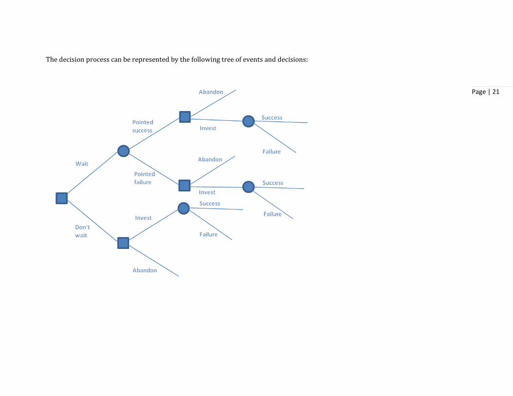
The decision process can be represented by the following tree of events and decisions:

Page | 22

Let us start by assigning asset values to the terminal branches (Success and Failure)

For instance, the success after investing without waiting gives 150+300=450, the failure gives 150-100=50.

The success after waiting and for a pointed success gives 150-30+300= 420, the failure gives 150-30-100=20.

Page | 23

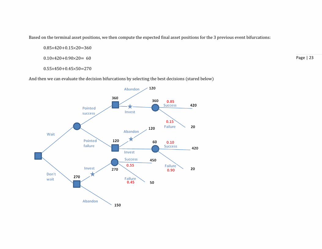
Based on the terminal asset positions, we then compute the expected final asset positions for the 3 previous event bifurcations:

0.85×420+0.15×20=360

0.10×420+0.90×20= 60

0.55×450+0.45×50=270

And then we can evaluate the decision bifurcations by selecting the best decisions (stared below)

Page | 24

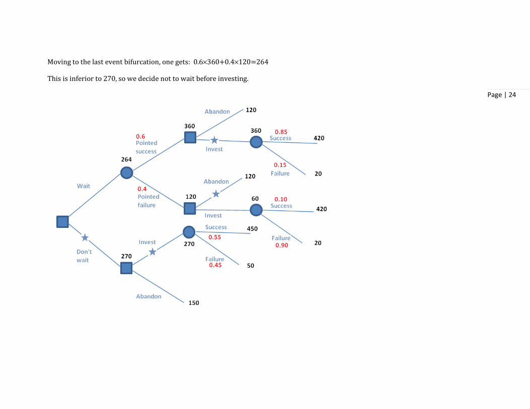
Moving to the last event bifurcation, one gets: 0.6×360+0.4×120=264

This is inferior to 270, so we decide not to wait before investing.

Page | 25

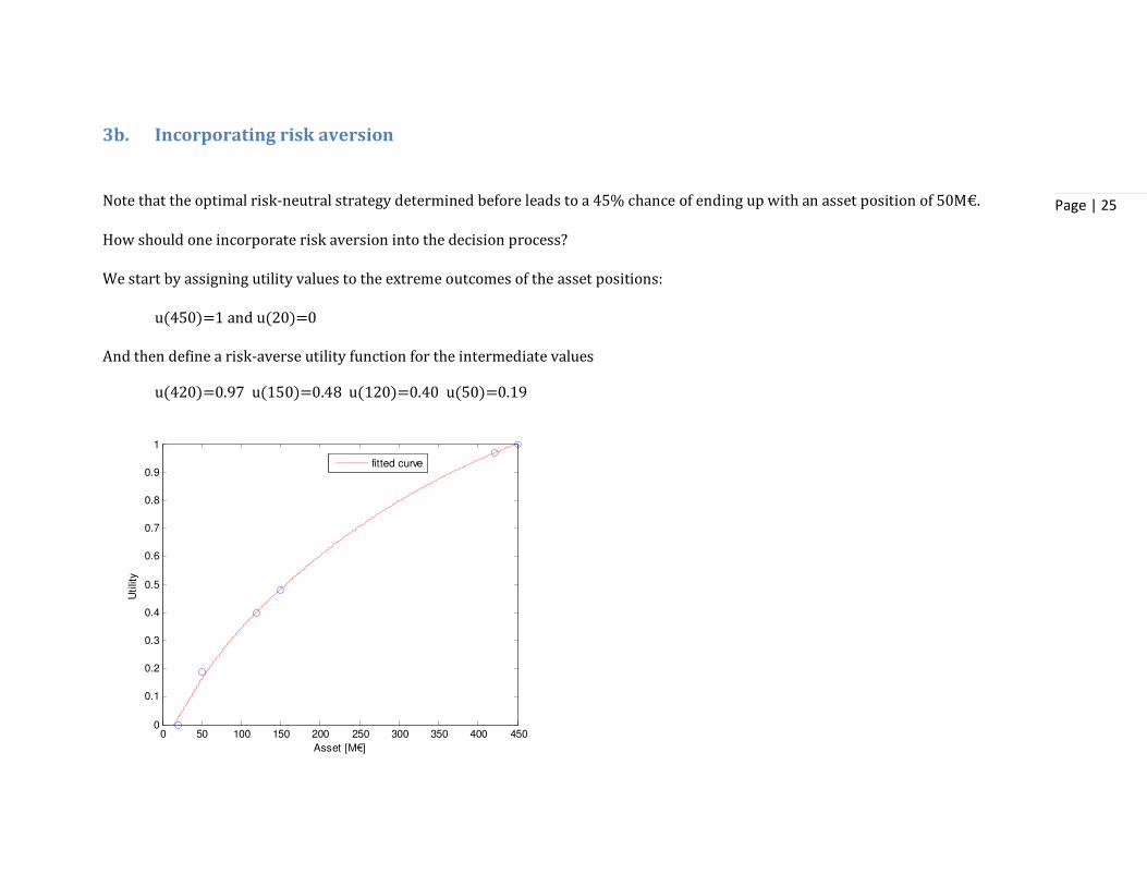
3b. Incorporating risk aversion

Note that the optimal risk-neutral strategy determined before leads to a 45% chance of ending up with an asset position of 50M€.

How should one incorporate risk aversion into the decision process?

We start by assigning utility values to the extreme outcomes of the asset positions:

u(450)=1 and u(20)=0

And then define a risk-averse utility function for the intermediate values

u(420)=0.97 u(150)=0.48 u(120)=0.40 u(50)=0.19

0 50 100 150 200 250 300 350 400 4500

0.1

0.2

0.3

0.4

0.5

0.6

0.7

0.8

0.9

1

Asset [M€]

Utilit

y

fitted curve

Page | 26

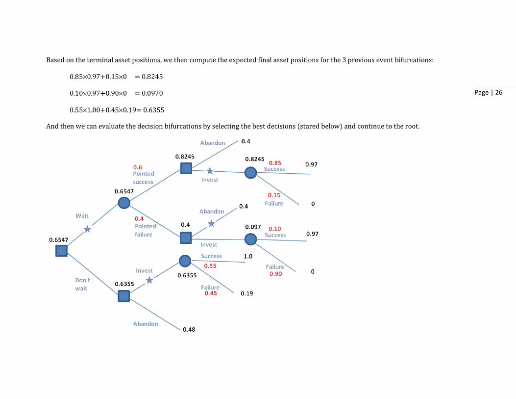
Based on the terminal asset positions, we then compute the expected final asset positions for the 3 previous event bifurcations:

0.85×0.97+0.15×0 = 0.8245

0.10×0.97+0.90×0 = 0.0970

0.55×1.00+0.45×0.19= 0.6355

And then we can evaluate the decision bifurcations by selecting the best decisions (stared below) and continue to the root.

Page | 27

3c. Bayes’ rule and decision trees

In the example above, there are two states (success S and failure F) which have different probabilities (0.55 and 0.45, respectively)

P(S)=0.55

P(F)=0.45

Let us call such probabilities, prior probabilitiesprior probabilitiesprior probabilitiesprior probabilities

But there are other probabilities for the transitions in the tree… those are dependent of the state, such as the probability of success S after a pointed success pS, which we write as P(S |pS)=0.85. Such probabilities are called posterior probabilitiesposterior probabilitiesposterior probabilitiesposterior probabilities....

P(S |pS)=0.85 P(S |pF)=0.10

P(F |pS)=0.15 P(F |pF)=0.90

However, sometimes we don’t have information on posterior probabilitiesposterior probabilitiesposterior probabilitiesposterior probabilities but instead information on likelihoods of each state given some prior information (observation). For example, we might know that:

• 55 investments that were a success have been decided after waiting; • from such 55 successes only 51 were pointed out as such.

Page | 28

The likelihoodslikelihoodslikelihoodslikelihoods can then be written as:

P(pS |S)=51/55

P(pF |S)=4/55

Suppose that one also has information on 45 failed investments and gets

P(pS |F)=9/45

P(pF |F)=36/45

To complete the decision tree, we still need the posterior probabilities, which we can get with help from the Baye’s ruleBaye’s ruleBaye’s ruleBaye’s rule:

JKLMNOPQ =J(LM ∩ OP)

J(OP)=

JKOPNLMQJ(LM)∑ JKOPNLTQU

TVW

One gets

J(YL ∩ L) = P(pS |S) P(S)=51/55(0.55)=0.51

J(YZ ∩ L) = P(pF |S) P(S)= 4/55(0.55)=0.04

J(YL ∩ Z) = P(pS |F) P(F)= 9/45(0.45)=0.09

J(YZ ∩ Z) = P(pF |F) P(F)=36/45(0.45)=0.36

And

J(YL) = J(YL ∩ L) + J(YL ∩ Z) = 0.51 + 0.09 = 0.6

J(YZ) = J(YZ ∩ L) + J(YZ ∩ Z) = 0.04 + 0.36 = 0.4

Page | 29

Which can be used to compute the posterior probabilities:

P(S |pS)=0.51/0.6=0.85

P(S |pF)=0.04/0.4=0.10

P(F |pS)=0.09/0.6=0.15

P(F |pF)=0.36/0.4=0.90

Page | 30

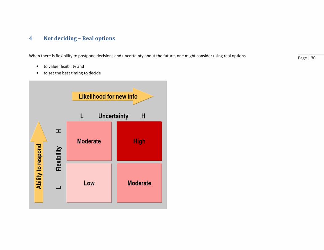
4 Not deciding – Real options

When there is flexibility to postpone decisions and uncertainty about the future, one might consider using real options

• to value flexibility and

• to set the best timing to decide

Page | 31

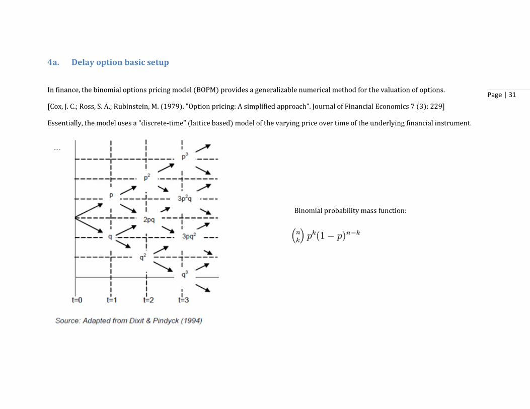
4a. Delay option basic setup

In finance, the binomial options pricing model (BOPM) provides a generalizable numerical method for the valuation of options.

[Cox, J. C.; Ross, S. A.; Rubinstein, M. (1979). "Option pricing: A simplified approach". Journal of Financial Economics 7 (3): 229]

Essentially, the model uses a “discrete-time” (lattice based) model of the varying price over time of the underlying financial instrument.

Binomial probability mass function:

Page | 32

4b. Pricing an option

STEP 1: Create the binomial price tree

The tree of prices is produced by working forward from valuation date to expiration.

At each step, it is assumed that the price will move up or down by a specific factor ( or ) per step of the tree. So, if is the current

price, then in the next period the price will either be

or

.

The up and down factors are calculated using the underlying volatility, , and the time duration of a step, , measured in years. From

the condition that the variance of the log of the price is , we have:

This property also allows that the value of the underlying asset at each node can be calculated directly via formula, and does not

require that the tree be built first. The node-value will be:

Where is the number of up ticks and is the number of down ticks.

Page | 33

STEP 2: Find Option value at each final node

At each final node of the tree, i.e. at the expiration date of the option, the option value is simply its intrinsic, or exercise, value.

Max { , 0} for a call option

Max { – , 0} for a put option:

Where is the strike price and is the spot price of the underlying asset at the period.

STEP 3: Find Option value at earlier nodes

Once the above step is complete, the option value is then found for each node, starting at the penultimate time step, and working back

to the first node of the tree (the valuation date) where the calculated result is the value of the option.

In overview: the “binomial value” is found at each node, using the risk neutrality assumption. The steps are as follows:

(1) Under the risk neutrality assumption, today's fair price of a derivative is equal to the expected value of its future payoff discounted

by the risk free rate. Therefore, expected value is calculated using the option values from the latter two nodes (Option up and Option

down) weighted by their respective probabilities—“probability” p of an up move in the underlying, and “probability” (1-p) of a down

move. The expected value is then discounted at r, the risk free rate corresponding to the life of the option.

Where

is the option's value for the node at time , and

Page | 34

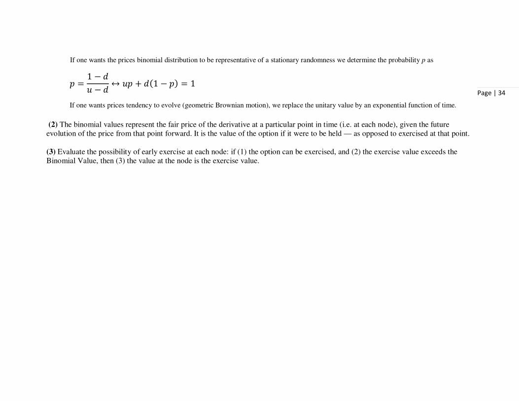
If one wants the prices binomial distribution to be representative of a stationary randomness we determine the probability p as

Y =1 − ab − a

↔ bY + a(1 − Y) = 1

If one wants prices tendency to evolve (geometric Brownian motion), we replace the unitary value by an exponential function of time.

(2) The binomial values represent the fair price of the derivative at a particular point in time (i.e. at each node), given the future

evolution of the price from that point forward. It is the value of the option if it were to be held — as opposed to exercised at that point.

(3) Evaluate the possibility of early exercise at each node: if (1) the option can be exercised, and (2) the exercise value exceeds the

Binomial Value, then (3) the value at the node is the exercise value.

Page | 35

Example:

Page | 36

Page | 37

p 0,40 up prob.

q 0,60 (1-p)

r 0,10 risk free discount rate

s 300 initial asset position

u 1,5 up factor (down factor=1/u)

i 375,00 investment

probabilities

1,0000 0,4000 0,1600 0,0640

0,6000 0,4800 0,2880

0,3600 0,4320

0,2160

asset position

300 450 675,0 1012,5

200 300,0 450,0

133,3 200,0

88,9

i option value 29,1 80,4 245,6

0,0 0,0

0,0

The red colored figure means that the figure results from exercising the

option, i.e., making the investment. Other figures result from waiting for

investing (if not zero) or abandoning the investment option (zeros)