energy and material balances of wastewater treatment...
TRANSCRIPT

Linköping University | Department of Management and Engineering
Master’s thesis, 30 credits| Master’s programme in Energy and Environmental Engineering
Spring 2016| ISRN-number: LIU-IEI-TEK-A--16/02676—SE
Energy and material balances of wastewater treatment, including biogas production, at a recycled board mill
Igor Assis Lana e Cruz
Supervisor: Magnus Karlsson / IEI, Linköping University
Company Supervisor: Magnus Johanson / Fiskeby Board AB
Examiner: Maria Johansson / IEI, Linköping University
Linköping University
SE-581 83 Linköping, Sweden
+46 013 28 10 00, www.liu.se

I
Abstract
Challenges surrounding energy have gained increased attention, which is not least reflected in the 2030 Agenda for Sustainable Development and the Sustainable Development Goals (SDGs). Energy issues have also become a pressing matter for most countries in the last decades. The reasons for this are not only related to the effects of the emission of greenhouse gases (GHG) from fossil fuels and their impact in climate change, but also span through other issues such as security of energy supply with geopolitical considerations and competitiveness of industry. To address these issues, a collection of public policies ranging from the international to local levels have been implemented.
Sweden has historically had lower energy prices than its European counterparts, which has resulted in its industry having a relatively higher share of electricity in the total energy use by industry. The share of electricity accounts for 35% of total energy use in Swedish industry. This has led to efficiency measures being overlooked by industry, and the pulp and paper industry is by far the biggest energy user, with a share of 51% of the total energy use by industry. The variation of energy prices, and particularly electricity prices have obvious implications on the competitiveness of this sector.
Production of biogas in pulp and paper mills has been gaining attention, and is now the target of an increasing number of scientific studies. The interest for this industry is not only related to security of energy supply and the environmental performance of the biogas itself, but there are also considerations regarding the biogas plant as an alternative to treat the large flows of wastewaters and other waste stream in this sector. There is an estimated biogas production potential of 1 TWh within this industry in Sweden, which accounts for 60% of the current biogas production in the country.
Pulp and paper mills commonly rely on aerated biological treatment to deal with waste streams with high organic content This biological process has a high energy demand, and the integration of an anaerobic treatment, along with the use of the biogas for heat and electricity can yield a net positive energy recovery for the combined plant.
This project analyses the current energy and material performance of an anaerobic biological treatment combined with an aerobic biological treatment in a recycled board mill. The anaerobic treatment is performed upstream of the aerobic one and removes most of the chemical oxygen demand of the wastewater.
Energy and material balances for the plant are presented, and a comparison of the wastewater treatment plant running before and after the start-up of the biogas plant is made. The plant operation with the anaerobic digestion has shown an increased energy use of 9.4% coupled to an increased flow of wastewater of 7.7%. The average biogas production is 72 Nm³/h, which accounts for 440 kWh and is currently being flared. The introduction of AD has largely decrease the organic load in the aerobic treatment, by nearly 50%. This project ends with an optimisation model implemented with the optimisation tool reMIND to investigate potential optimisation strategies for the operation of the combined plant. The model has shown to be adequate to describe electricity use with mean error below 10%. For the biogas production, the mean error was of 16%.


III
Acknowledgements
This thesis is the final work in my Master’s Programme in Energy and Environmental Engineering at Linköping University (LiU), Sweden. The work is part of one of the three case studies under development within the quantitative systems research project area in the Biogas research centre (BRC) of LiU. The specific case study focuses on biogas production at pulp and paper mills. The work was done at Fiskeby Board AB, in Norrköping, Sweden, between March and August of 2016, and covers 30 credits within the master’s programme.
The supervisor in the company was Magnus Johanson, process development engineer. Magnus Karlsson, associate professor in the Energy Systems department was the supervisor at the university. I would like to thank both supervisors for sharing their knowledge and careful advice offered during the project, which was primordial to the completion of this thesis.
In addition, I would also like to give my compliments to the staff of Fiskeby Board AB for the opportunity and support, especially to Rickard Stark and Annelie Niva, members of the steering group within the company, and Lars-Åke Nilsson, who provided me with a lot of information with his broad experience in the operation of the wastewater treatment plant.


V
Table of Contents
Abstract ....................................................................................................................................... I
1 Introduction ....................................................................................................................... 1
1.1 Pulp and paper industry and biogas production ......................................................... 2
2 Objective ............................................................................................................................ 3
2.1 Research questions ..................................................................................................... 3
3 Case study .......................................................................................................................... 4
3.1 Company overview ...................................................................................................... 4
3.2 Recycled board production ......................................................................................... 5
3.3 Pulp preparation ......................................................................................................... 6
3.4 Wastewater treatment plant ...................................................................................... 7
3.4.1 The aerobic step ................................................................................................... 7
3.4.2 The flotation unit ................................................................................................. 9
3.4.3 The anaerobic digester (AD) ................................................................................ 9
3.4.4 Thiopaq biological scrubber ............................................................................... 11
3.4.5 Wastewater characterisation ............................................................................ 12
3.4.6 Current wastewater treatment plant process control ...................................... 13
3.4.7 Emission limits for the wastewater treatment plant ......................................... 14
4 Theory .............................................................................................................................. 15
4.1 Anaerobic process ..................................................................................................... 15
4.1.1 Up flow anaerobic sludge bed (UASB) reactor .................................................. 16
4.2 Performance evaluation in biogas production .......................................................... 16
4.2.1 Parameters and performance indicators ........................................................... 17
5 Method ............................................................................................................................ 20
5.1.1 System boundaries ............................................................................................. 20
5.1.2 Unit processes .................................................................................................... 21
5.1.3 Data collection ................................................................................................... 22
5.1.4 Recorded parameters ........................................................................................ 22
5.2 Energy and material balances ................................................................................... 23
5.2.1 Calculations for the energy balance .................................................................. 23
5.3 Energy system analysis and optimisation tool (reMIND) .......................................... 24
5.3.1 Mathematical programming and optimisation ................................................. 24
5.3.2 reMIND ............................................................................................................... 25

VI
5.4 Literature review ....................................................................................................... 26
6 Results and discussion ..................................................................................................... 27
6.1 Initial considerations ................................................................................................. 27
6.2 Material and flow measurements ............................................................................. 30
6.2.1 Before biogas commissioning ............................................................................ 30
6.2.2 After biogas commissioning ............................................................................... 33
6.3 Energy measurements .............................................................................................. 36
6.3.1 Before biogas commissioning ............................................................................ 36
6.3.2 After biogas commissioning ............................................................................... 38
6.4 Energy and material balances ................................................................................... 40
6.5 Reflection on the energy and material balances ...................................................... 44
6.6 reMIND model ........................................................................................................... 45
6.6.1 Input parameters ............................................................................................... 45
6.6.2 Built model ......................................................................................................... 50
7 Conclusion ........................................................................................................................ 53
Future studies .......................................................................................................................... 55
References ............................................................................................................................... 56
Appendices ............................................................................................................................... 59
Appendix A ........................................................................................................................... 59
Appendix B ........................................................................................................................... 63
Appendix C ........................................................................................................................... 64
Appendix D ........................................................................................................................... 65
Appendix E ........................................................................................................................... 66

VII
List of acronyms
AD Anaerobic digestion
BAT Best available technology
BOD Biochemical oxygen demand
COD Chemical oxygen demand
CTMP Chemical thermo-mechanical pulp
EU European Union
GHG Greenhouse gases
HW Hardwood
LOESS Locally weighted scatterplot smoothing
MILP Mixed Integer Linear Programming
MIND Method for analysis of INDustrial energy systems
SD Standard deviation
SDGs Sustainable Development Goals
SGP Specific biogas production
SLR Sludge (biomass) loading rate
SS Suspended solids
SW Softwood
TOC Total organic carbon
TSS Total suspended solids
UASB Up flow anaerobic sludge bed reactor
UNFCCC United Nations Framework Convention on Climate Change
VFAs Volatile fatty acids
VLR Volumetric loading rate

VIII
List of figures and tables
Figure 1: Overview of the energy balance for Fiskeby Board AB in 2013. Source: (Fiskeby Board AB, 2016), adapted. ................................................................................................................... 5
Figure 2: Different layers for the Multiboard production. Source: (Fiskeby Board AB, 2016). . 5
Figure 3: MS drum at Fiskeby Board AB. Source:(Jonsson & Kronqvist, 2014). ........................ 6
Figure 4: Schematic view of a sludge dewatering centrifuge. Source:(Hiller SP, 2016). ........... 8
Figure 5: Schematic of the UASB reactor with internal circulation. 1) Wastewater inlet. 2) Lower chamber with granular biomass. 3) First phase separator. 4) Gas riser. 5) Gas-liquid separator. 6) Effluent downer. 7) Upper chamber. 8) Second phase separator. 9) Wastewater outlet. 10) Tank ventilation. 11) Biogas outlet. 12) Sludge removal manifold. ....................... 10
Figure 6: Schematic representation of the Thiopaq process. Source: (Paques bv, 2015), adapted. ................................................................................................................................... 12
Figure 7: Simplified process diagram with main control parameters. Source: Fiskeby Board (2015). ...................................................................................................................................... 13
Figure 8: UASB reactor schematic representation. Source: (Tilley et al., 2014). .................... 16
Figure 9: Simplified process description with system boundaries .......................................... 21
Figure 10: Motor efficiency versus motor load for motors of different power. Source: (Bonneville Power Administration, 2005) ................................................................................ 24
Figure 11: Model example of a pulp and paper mill using the reMIND software (Karlsson, 2010). ....................................................................................................................................... 26
Figure 12: Average monthly temperature of the Motala river for the period 2001 - 2011. Source: (Jonsson & Kronqvist, 2014), adapted. ....................................................................... 27
Figure 13: Daily average wastewater temperature inflow for the wastewater treatment plant. The green line indicates the start of the AD. ........................................................................... 28
Figure 14: Daily average of incoming wastewater pH. The green line indicates the start of the AD. ............................................................................................................................................ 28
Figure 15: Suspended solids in the incoming wastewater. The green line indicates the start of the AD. ..................................................................................................................................... 29
Figure 16: Suspended solids in the outflow of treated wastewater to the river. The green line indicates the start of the AD. ................................................................................................... 29
Figure 17: Total organic carbon in the incoming wastewater, daily values. The green line indicates the start of the AD. ................................................................................................... 30
Figure 18: Flows in the aeration basin for the wastewater treatment plant before biogas commissioning. ........................................................................................................................ 31
Figure 19: Flows in the sedimentation basin for the wastewater treatment plant before biogas commissioning. ........................................................................................................................ 31
Figure 20: Flows in the centrifuge for the wastewater treatment plant before biogas commissioning. ........................................................................................................................ 32

IX
Figure 21: Flows in the flotation for the wastewater treatment plant before biogas commissioning. ........................................................................................................................ 32
Figure 22: Flows in the biogas plant for the wastewater treatment plant. ............................ 33
Figure 23: Flows in the aeration basin for the wastewater treatment plant. ......................... 34
Figure 24: Flows in the sedimentation basin for the wastewater treatment plant. ............... 35
Figure 25: Flows in the centrifuge for the wastewater treatment plant................................. 35
Figure 26: Flows in the flotation for the wastewater treatment plant. .................................. 36
Figure 27: Total energy use (kWh) per day for each treatment step, grouped by unit process, before biogas commissioning. ................................................................................................. 37
Figure 28:Total energy use (kWh) per day for the biogas and aeration steps, grouped by unit process, current situation. ....................................................................................................... 38
Figure 29: Total energy use (kWh) per week for the sedimentation, centrifuge and flotation steps, grouped by unit process, current situation. .................................................................. 39
Figure 30: Energy and mass balance for the plant before biogas comissioning, daily averages................................................................................................................................................... 41
Figure 31: Current energy and mass balance for the plant, daily averages. The energy use per unit process is given in average energy use per day. .............................................................. 42
Figure 32: COD removed in each step of the treat process. Absolute values per hour, average hourly removal, taken daily (right,), and the proportion of the total COD (left). ................... 44
Figure 33: Expected gas production with COD removed versus actual production (up), and biogas potential by TOC removed versus actual production (down). The areas are coloured to show the overlap. .................................................................................................................... 45
Figure 34: pH and temperature in the incoming wastewater, buffer tank and AD reactor. The black lines show the ideal limits for these parameters. .......................................................... 46
Figure 35: Pearson correlation matrix for parameters in the biogas reactor. ........................ 47
Figure 36: Correlations in pair of parameters for inputs and outputs of the biogas plant. Diagonals are frequency distributions. Subscript “_ad” is a parameter leaving the plant. .... 47
Figure 37: Scatter plots of COD removal efficiency x COD load and flow, for the aerobic treatment, excluding flotation. COD_aer represents the COD load to the aerobic treatment and n_eff the removal efficiency. ............................................................................................ 48
Figure 38: Correlation between efficienccy of flotation x COD load, flow. COD is the COD load to the flotation, n_eff the COD removal efficiency of this step. ............................................. 49
Figure 39: reMIND model for the wastewater treatment plant. Blue flows are wastewater, red COD load, black are dried aearated sludge from the centrifuge and anaerobic sludge from the AD reactor, respectively. Yellow lines are electricity supply and green biogas produced. The node for the AD reactor includes the scrubber. ...................................................................... 50
Table 1: Biopaq IC Reactor. Source: (Paques bv, 2014) ........................................................... 10
Table 2: Process parameters of the anaerobic digester. ......................................................... 11

X
Table 3: Wastewater streams included in the screening of biomethane potentials within pulp and paper mills. The biomethane potentials given are mean values ± standard deviation (SD) of triplicates. Abbreviations: CTMP=chemical thermo-mechanical pulp, SW=softwood, HW=hardwood, Rec. fibre=recovered fibre and pre-sed.=pre-sedimentation. Source: (Larsson, 2015), adapted. ........................................................................................................ 13
Table 4: Emissions limits for Fiskeby Board AB. Source: (Fiskeby Board AB, 2016). ............... 14
Table 5: Average daily mass flows in the wastewater treatment plant for both periods analysed. .................................................................................................................................. 43
Table 6: Average energy use per day for both periods analysed. ........................................... 44
Table 7: Correlation between process parameters and TOC for the period analysed ............ 46
Table 8: Input parameters for the reMIND model. ................................................................. 49
Table 9:Validation of model results with the energy and mass balance obtained. ................ 50
Table 10: Measurements for each day and simulation results. M_number identifies the measured value and S_number idenfies the simulation results. ............................................ 52

1
1 Introduction
At a global level, the challenges surrounding energy have gained increased attention, which is not least reflected in the 2030 Agenda for Sustainable Development and the Sustainable Development Goals (SDGs) – and in particular goal 7: “Ensure access to affordable, reliable, sustainable and modern energy for all” and its related targets (Sustainable Development Platform, 2015).
Energy issues have also become a pressing matter for most countries in the last decades. The reasons for this are not only related to the effects of the emission of greenhouse gases (GHG) from fossil fuels and their impact in climate change, but also span through other issues such as security of energy supply with geopolitical considerations (Correljé & van der Linde, 2006) and competitiveness of industry due to fluctuations in energy prices (European Comission, 2014). To address these issues, a collection of public policies ranging from the international to local levels have been implemented which focus on each of these. In an environmental perspective the most prominent international policy is the Kyoto Protocol, which has established targets on reduction of GHG emissions for the base year of 1990 for signatory countries with legally binding targets for the countries under its annex B, which are all high-income countries (UNFCCC, 1997). For most signatory European Union (EU) countries, including Sweden, the binding target for the first period of the protocol (2008-2012) was the reduction of 8% of GHG emissions for the base year 1990. Nevertheless, European countries have agreed on a burden sharing scheme in which different goals applied to each member state to achieve a common communitarian goal (Europeiska miljöbyrån, 2004).
The Renewable Energy Directive of the EU has set goals for its member states requiring a 20% reduction of GHG emissions, 20% share of renewable energy in its gross final energy consumption1 and 20% increase in energy efficiency by the year 2020 in comparison to the base year of 2005 (European Parliament, 2009).
Sweden has historically had lower energy prices than its European counterparts, which has resulted in its industry having a relatively higher share of electricity in the total energy use by industry (Thollander, 2008), while as well having an exceptionally high level of bioenergy. The shares of bioenergy and electricity account for 38% and 35% of total energy use in Swedish industry, respectively (Swedish Energy Agency, 2015). This has led to efficiency measures, previously, being overlooked by industry, but the participation in the European block market for energy and new energy policies resulted in increasing prices, which are now a pressing factor for competitiveness (Cipollone & Zachmann, 2013).
In the Swedish context, the pulp and paper industry is by far the biggest energy user, with a share of 51% of the total energy use by industry (Swedish Energy Agency, 2015). The variation of energy prices, and particularly electricity prices have obvious implications on the competitiveness of this sector of industry. In addition, the sector has struggled in the
1 In the context of the EU energy policy directives the term energy consumption is used, although academically the preferred term, and the one used in this work, is energy use.

2
European market, with locally decreasing demand in some sectors and competition for resources (The Environmental Paper Network, 2015).
1.1 Pulp and paper industry and biogas production
The pulp and paper industry is a new biogas producer in Sweden and other countries. Production of biogas in paper and pulp mills is not only related to the interest in finding alternative energy sources, increasing energy security and increased competition in the industry, but is also related to the opportunity to treat flows of wastewater and comply with environmental regulations regarding the emission of pollutants. For the pulp and paper industry, which is a large energy user and generates relatively large amounts of wastewater needed for the process, the opportunity to treat waste flows to desirable standards is a main driver for looking into biogas production, with the potential energy benefits of such measures still being overlooked (Olsson & Fallde, 2015).
As a new area of interest for the pulp and paper industry, the pulp and paper industry has been the target of an increasing number of scientific studies, centring the systematic impact of current energy and environmental issues on these types of biogas installations in Sweden. See, for example, the work of Larsson (2015), in which the biogas potential of wastewaters from several Swedish pulp and paper mills was investigated, and the work of Magnusson and Alvfors (2012), which goes in the same line. The demand for improved biogas production and the need of a greater geographical distribution of biomethane sources intensify the interest of adopting biogas plants integrated into pulp and paper productions sites. Magnusson and Alvfors (2012) have estimated a biomethane potential of 1TWh within this industry in Sweden, which accounts for approximately 60% of the Swedish biogas production in 2015 (Larsson, 2015).
Commonly the industry relies on aerated biological treatments to deal with the large flows of wastewater with high organic content, which are large electricity users (Meyer & Edwards, 2014). The integration of an anaerobic treatment plant and the use of biogas for heat or electricity production can yield a net positive energy recovery for the combined wastewater treatment plant (Larsson, 2015).
Another factor to take into consideration is the fact that the Swedish pulp and paper industry has decreased in number of mills by about 40% in the last three decades, to around 50 mills in 2015, while the average capacity of each plant has more than doubled over the same period (Swedish Forest Industries Federation, 2015). In this scenario, the capacity of traditional wastewater treatment facilities is stressed and the need for investment in upgrades in capacity opens up an opportunity to new technologies to be introduced.
Worldwide, less than 10% of all mills have implemented anaerobic digestion (AD) as a treatment method for their wastewater, even though this number has doubled in the last decade (Meyer & Edwards, 2014). In Sweden, there are currently only two mills using AD: Domsjö Fabriker AB, a sulphite pulp mill treating only 10% of the total wastewater of the mill by AD, and Fiskeby Board AB, a recycled board mill where the total effluent of the mill is treated prior to the aerobic treatment (Larsson, 2015).
As it can be seen, the potential for biogas production within the Swedish pulp and paper industry is of relevance in several aspects, and this study covers an energy and material balance of a combined anaerobic and aerobic treatment plant installed at Fiskeby Board AB, with a further study on strategies to properly integrate the two technologies.
3
2 Objective
In this study, energy and material balances for the wastewater treatment plant at Fiskeby Board AB are used as a case study and a model with the optimisation methodology reMIND is built. The aim is to analyse the efficiency of the plant on the basis of the energy and material balances. Critical factors and uncertainties in input data and results are made visible in the analysis. Particularly, one uncertainty in focus are the variations in the organic material from the recycled board mill to be digested and its influence on the biogas production. Where possible, comparisons with other similar biogas production plants linked to a pulp and paper mill will be carried out after a literature research to determine the similarities and differences of such plants. Efficiencies of the plant in terms of proportion of removal of the chemical oxygen demand (COD) load, biogas yield versus COD load and energy uses are considered. In order to fulfil these objectives, research questions are imposed and answered.
2.1 Research questions
What is the current energy and material balance for the wastewater treatment plant at
Fiskeby Board AB?
Is the chosen energy system analysis and optimisation tool (reMIND) adequate to describe the
process in an industrial level for the wastewater treatment plant at Fiskeby Board AB?
How do the fluctuations of input influence the output of the biogas plant for the wastewater
treatment plant at Fiskeby Board AB?
What are the potential process control and optimisation measures to be adopted by the use
of the reMIND model or insights given by the analysis of the energy and material balances for
the wastewater treatment plant at Fiskeby Board AB?

4
3 Case study
3.1 Company overview
Fiskeby Board is a recycled board mill situated in Norrköping, Sweden, owned by Fiskeby Holdings LLC USA. Established in 1637, the company is the only one board mill in Scandinavia producing from 100% recovered fibre. Its current board machine started operation in 1953 and was rebuilt in 1987, currently with an installed capacity of 170 000 tons per year. With 258 employees, the company has been increasing its production over time, currently producing 160 000 tons per year of recycled board in a range of six main different products, marketed with a product name of Multiboard. The current permit allows the company to produce 200 000 tons of recycled board.
Multiboard versions are called Multiboard Offset, EcoFrost, Kraft, Ecokraft, Barrier and Premium. Of the total production, 130 000 tons are sold as sheeted product, and 16 000 tons run through the extrusion line, where a plastic coating of the board is added for special food packaging applications. The main market for the company is the food packaging industry, with clients concentrated mostly in Germany, United Kingdom, Sweden and other northern European countries. Customers include Unilever, Nestlé, Procter & Gamble, Mondeléz and others (Fiskeby Board AB, 2016). ISO 9001, ISO 14001 and ISO 50001 for quality, energy and environmental management are some of the certifications under which the company is accredited.
As part of its waste and energy management plan, the company has invested in a waste to energy facility, installed in 2010, which generates 100% of the steam demand and up to 40% of the electricity demand.
Recently, the company has started the operation of a biogas reactor as part of the wastewater treatment plant, which was commissioned in August 2015. The choice of the anaerobic treatment is related to the internal confidence within the company in biological treatment of wastewater, as the plant personnel is experienced in the aerobic treatment traditionally used. Additionally, the technology was chosen to fit the best available technology (BAT) as demanded by ordinance 2013:250 of the Swedish Parliament, which sets requirements and limits on industrial emissions divided by sector branch. This regulation is derived from the Industrial Emissions Directive 2010/75 EU, passed by the European parliament (Sveriges Riksdag, 2013). The main driver for the adoption of the anaerobic treatment is the reduction of the COD of the wastewater generated during production, followed by an aerobic treatment step to further improve the effluent characteristics. This allows the company to increase recycled board production while staying within emission limits as per the permissions granted by the Swedish Environmental Court (Miljödomstolen). An overview of the mill’s energy balance for 2013 is presented in Figure 1.

5
Figure 1: Overview of the energy balance for Fiskeby Board AB in 2013. Source: (Fiskeby Board AB, 2016), adapted.
3.2 Recycled board production
The Multiboard board is composed mainly of four different layers with different grades of recycled fibre, which go through different pulp preparation steps prior to the board machine, and are chosen according to their mechanical and chemical properties. The top, under and back layers are formed by pre-consumer recovered fibre and have a smaller thickness than the middle layer, which is formed by post-consumer recovered fibre. Coating, top coating and pre coating are added to some of the product ranges to meet different quality requirements. Figure 2 presents the layers used in the construction of the Multiboard.
Figure 2: Different layers for the Multiboard production. Source: (Fiskeby Board AB, 2016).

6
The four layers are formed at the beginning of the board machine (KM1), where pulps of different grades are added together. This section of the board machine is called wet end. Following in the process, the board goes to the press section where it is mechanically pressed by drums, including the use of vacuum pumps. This section increases the dry content of the forming board from 17% to 48%. After that the board follows to the dryer section in which it is heated up by means of drums warmed with steam, and the humidity content of the board is further decreased. After the dryer section, the coating section starts and the board receives layers of coating to each side. The underside of the surface receives a coating consisting of starch and clay. The coating has the objective of improving the smoothness of the surface and increase printability of it. After the coating, further drying is achieved by infrared dryers and hot air, after which the board is rolled up in tambours and follows to the sheeting department.
3.3 Pulp preparation
The middle layer (MS) is formed by post-consumer recovered fibre. It uses carton board and consumer food packaging such as milk and juice boxes. Fiskeby receives pallets of recovered material which are ground up in smaller pieces and fed mixed with water to a giant rotating drum (MS drum). The water dissolves the fibre content and then the drum separates plastic, aluminium and other contaminants from the paper fibre. The dissolved fibre is removed from the drum while the other materials separated stay in the drum and are extracted by its end. The dissolved fibre is sent to further processing while the extracted solid material is collected and sent to the boiler house. Figure 3 shows a picture of the MS drum installed at Fiskeby Board AB.
The further processing of the middle layer involves a coarse screen to remove large particles. The filtered fibre is then sent to a cyclone and disc filters, and the further selected fibre is collected to be injected in the board machine.
The pulp which forms the other layers is formed by pre-consumer recovered fibre, from both in-house production and other mills, and goes directly to the pulping machines, where the fibre is dissolved. For the under layer and back layer, a mix of post-consumer recovered fibre can be added.
Figure 3: MS drum at Fiskeby Board AB. Source:(Jonsson & Kronqvist, 2014).

7
3.4 Wastewater treatment plant
The wastewater treatment plant present at Fiskeby Board AB initially had only an aerobic treatment step followed by a flotation unit installed. This system was operating near the maximum of its capacity and became a main constraint to the plant operation as it could not cope anymore with an increase of the wastewater influx and keep the treated effluent within regulation and permit limits. In order to allow an increase of the wastewater generated as a result of an increased production, the anaerobic treatment was introduced to work as a primary step for the wastewater treatment plant, reducing the COD load which is handed over to the aerobic step. The idea is for both systems to work combined, allowing for a greater amount of wastewater treated. The anaerobic digestion plant started operation in the second semester of 2015. A detailed process flowchart is presented in Figure A 1 in Appendix A, showing the flows and equipment of the wastewater treatment plant as it is currently installed.
Table A 1 in the same appendix presents the definition and explanation of the process flowchart flow numbers.
3.4.1 The aerobic step
The current aerobic treatment plant was built in 1994 and was upgraded twice after that. In 2010, it received a new compressor for the aeration system in order to increase the aeration capacity of the aeration basin and improve digestion of the organic load to the plant. Even with the improvements, the plant is running close to its maximum capacity and a further upgrade would require major investments.
The aerobic treatment step is more complex and has more phases than an anaerobic one, but it basically includes an aeration basin, a sedimentation basin and a centrifuge to remove excesses of activated sludge. In this facility, the biggest energy users are the blowers required for proper aeration of the incoming wastewater, but pumping and the centrifuge also account for a relevant amount of the energy use.
3.4.1.1 Aeration basin
The wastewater may be delivered directly from the board machine or pass the anaerobic digester to the central section of the aeration basin, which contains plastic carriers of bacteria to start the aerobic decomposition of the COD load. Currently, at least 10% of the wastewater flow from the board machine is constantly added directly to the aerobic step in order to keep bacterial activity in a level high enough to handle higher COD loads due to stops, both planned and unplanned, in the anaerobic treatment. This is also the case when the wastewater coming from the board machine is out of specification for the anaerobic treatment. The main control for the wastewater to divert from the anaerobic treatment is the concentration of suspended solids, and in case it is too high all the wastewater is bypassed directly to the aerobic treatment to protect the anaerobic bacteria in the AD. In this context, the anaerobic bacterial culture is called biomass.
After the initial activation, the wastewater then flows to the outer section of the aeration basin, where large blowers and a powerful mixing equipment aerate the wastewater to the adequate oxygen levels. In this basin, phosphorous and urea are added as nutrients to the process mixed with a recirculation flow of activated sludge, which is extracted from the next step, the sedimentation basin. The total basin volume is 3300 m³. The ideal temperature for

8
the aeration basin to allow proper activation of the biomass is 34 to 36 °C, and a pH between 7 and 8. The typical flow when only the aerobic step is in operation is 170 m³/h of raw wastewater, whereas when AD is active only the base flow is maintained to allow bacterial activation, and the COD reduced wastewater from the AD is received, summing up to the same flow but with a much lower COD load.
3.4.1.2 Sedimentation basin
An overflow drain collects the oxygenated wastewater from the aeration basin, which is dosed with iron chloride and polymers and directed to the central section of the sedimentation basin. Iron chloride works as a coagulating agent and polymer is the flocculating agent. In the central section, flocculation takes place under agitation and the wastewater follows to the outer section of the sedimentation basin. In this basin, a higher residence time then in the aeration and the flocculated sludge formed due to the added chemicals allow the sludge to settle in the bottom of the basin. The activated sludge is removed by means of a bottom scrapper, and is then partially directed to a centrifuge, while most of it is sent back to the outer section of the aeration basin to degrade the incoming organic load of the wastewater. This activated sludge is dosed with phosphoric acid and urea with an automated control system to adjust the parameters of the water in the aeration basin. The sedimentation basin has a total volume of 3000 m³.
The overflow of the sedimentation basin is drained to a sump, where it can either leave the wastewater treatment plant if the water characteristics are adequate, or be directed to a third treatment step of flotation.
3.4.1.3 Centrifuge
The centrifuge is used for the removal of excess sludge from the aerobic step. It receives sludge-rich water coming from both the sedimentation basin and the flotation unit. There is also a small intermittent flow coming from a foam skimmer in the sedimentation basin. The centrifuge consists of a solid bowl, which rotates and contain the process water. A screw conveyor inside the solid bowl rotates at a lower speed and separates the sludge from the water. The incoming water is dosed with iron chloride and polymer to increase the efficiency of sludge removal. The activated sludge is dewatered and stored to be collected as refuse. The filtrate of the centrifuge, which still contains a proportion of the initial amount of solids entering the centrifuge, is collected into a sump and pumped back to the aeration basin by a submersible pump. A schematic view of a centrifuge is shown in Figure 4.
Figure 4: Schematic view of a sludge dewatering centrifuge. Source:(Hiller SP, 2016).

9
3.4.2 The flotation unit
The flotation unit was built in 2010 to increase the treatment capacity of the wastewater treatment plant.
After the anaerobic and aerobic steps, most of the COD load is removed from the wastewater. Depending on the wastewater characteristics, however, it might happen that a high amount of suspended solids remains in the process. When it is detected by online measurements that the amount of suspended solids in the wastewater leaving the sedimentation basin is too high, the flotation unit is started and the wastewater is directed there. In the flotation unit, iron chloride and polymers are added again to allow the coagulation and flocculation of the suspended solid particles and posterior flotation of the flocculated sludge.
The flotation unit has an incoming basin where the flocculation takes place, and the overflow of the flocculation is then sent to the flotation basin, where a mix of water and micro air bubbles are injected to allow the flotation, i.e. the solid particles are sent upwards by the small air bubbles in the floatation basin. The floating sludge is then removed by a surface scraper and temporarily stored until it is periodically pumped to the centrifuge. The underflow of the flotation basin is clean wastewater and leaves the wastewater treatment plant. Part of the underflow is pumped back to the air drum to be mixed with compressed air and be injected back into the system. The total volume for the third step, including the flocculation and flotation basins is 60 m³.
3.4.3 The anaerobic digester (AD)
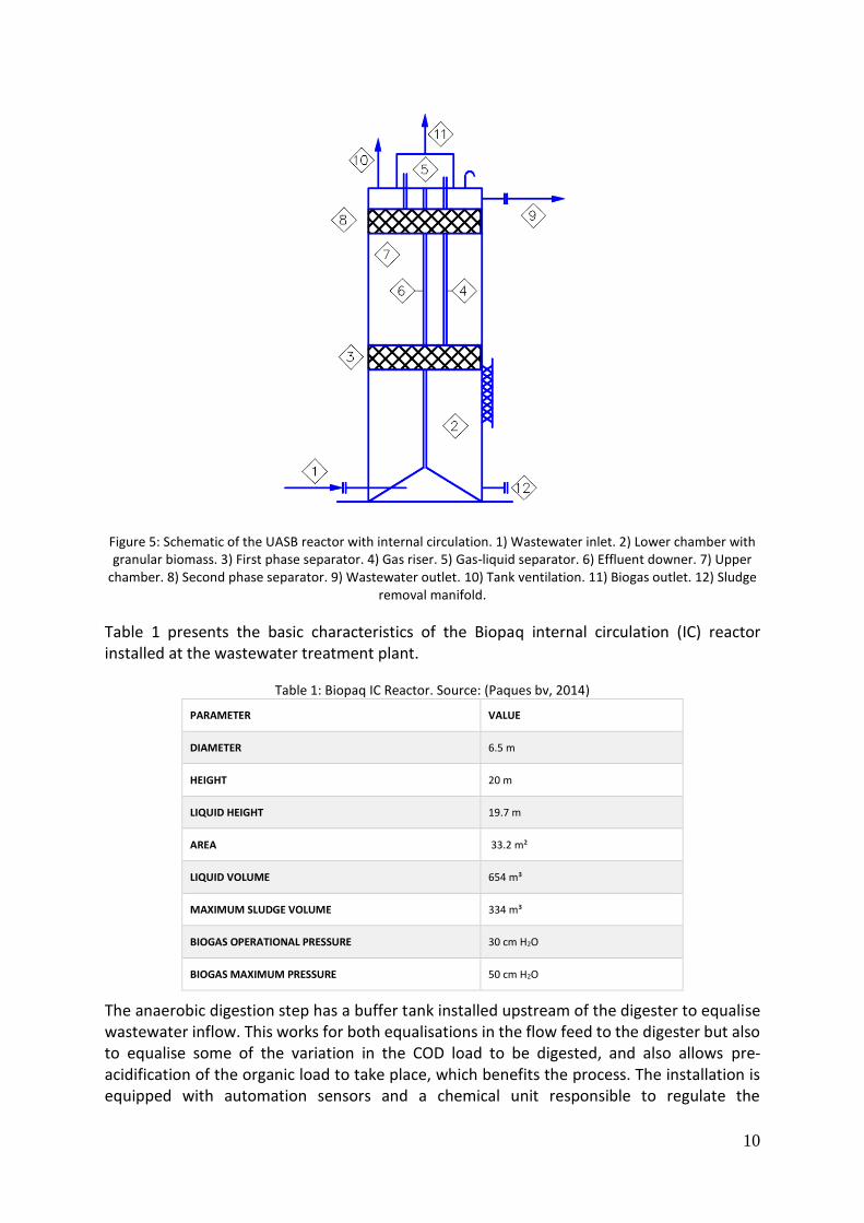
The anaerobic step at Fiskeby Board AB uses an up flow anaerobic sludge bed reactor (UASB) with internal recirculation. The UASB at Fiskeby is a Biopaq IC Reactor. This reactor works with a mesophilic process, with temperatures ranging ideally from 30 to 38 °C. The reactor has a volume of 654 m³ and typical residence time of about four hours. Influent water enters the digester at the bottom, and biogas and COD reduced wastewater are collected at the top. Internally the digester is formed by three compartments, separated by two phase separators, which collect the gas generated and let the upstream wastewater continue its rise to the top of the digester. Granular biomass sludge is normally present only in the lower compartment, where it is highly mixed with the influent water to allow adequate activation of the biomass and consequently increase the biological activity and biogas production. Figure 5 shows a schematic view of the anaerobic digester, with the description of its sections.
10
Figure 5: Schematic of the UASB reactor with internal circulation. 1) Wastewater inlet. 2) Lower chamber with granular biomass. 3) First phase separator. 4) Gas riser. 5) Gas-liquid separator. 6) Effluent downer. 7) Upper
chamber. 8) Second phase separator. 9) Wastewater outlet. 10) Tank ventilation. 11) Biogas outlet. 12) Sludge removal manifold.
Table 1 presents the basic characteristics of the Biopaq internal circulation (IC) reactor installed at the wastewater treatment plant.
Table 1: Biopaq IC Reactor. Source: (Paques bv, 2014)
PARAMETER VALUE
DIAMETER 6.5 m
HEIGHT 20 m
LIQUID HEIGHT 19.7 m
AREA 33.2 m²
LIQUID VOLUME 654 m³
MAXIMUM SLUDGE VOLUME 334 m³
BIOGAS OPERATIONAL PRESSURE 30 cm H2O
BIOGAS MAXIMUM PRESSURE 50 cm H2O
The anaerobic digestion step has a buffer tank installed upstream of the digester to equalise wastewater inflow. This works for both equalisations in the flow feed to the digester but also to equalise some of the variation in the COD load to be digested, and also allows pre-acidification of the organic load to take place, which benefits the process. The installation is equipped with automation sensors and a chemical unit responsible to regulate the

11
concentration of chemicals to its optimal levels. Urea and phosphoric acid are automatically dosed to the buffer tank. The pH of the incoming wastewater is also regulated by this system through the addition of sodium hydroxide (NaOH). There is no active temperature control in the system. Table 2 presents the operation requirements and other parameters for the Biopaq IC reactor.
The produced biogas is then sent to a biological scrubber (Paques Thiopaq).
Table 2: Process parameters of the anaerobic digester.
PARAMETER VALUE
FLOW RANGE 140-265 m³/h
RESIDENCE TIME ~4 h
BIOMASS CONCENTRATION 250 (max) g/l TSS
INORGANIC MATTER 50-60 (max) % TSS
SPECIFIC BIOGAS PRODUCTION 0.35-0.65 m³ biogas/ kg COD removed
PRE ACIDIFICATION LEVEL 30-50 %
VFAEFFLUENT <5 – 10 meq/l
OPERATIONAL PH 6.5-8.0
ALKALINITY 15 (min) meq/l
TEMPERATURE 25-40 °C (30-38 °C optimum)
NITROGEN (N) >5 mg/l effluent
PHOSPHATE (P) >1 mg/l effluent
CALCIUM (CA) 50-600 mg/l
MAGNESIUM (MG) 10-20 mg/l
POTASSIUM (K) 20:1 Na+ : K+ [mol]
3.4.4 Thiopaq biological scrubber
The Thiopaq installation removes hydrogen sulphide (H2S), a highly toxic gas even at extremely low concentrations (See Table B 1 in Appendix B).
The hydrogen sulphide is washed in by an alkaline water solution and then converted biologically into elemental sulphur. The sulphur is separated from the liquid by sedimentation. The Thiopaq installation is shown schematically in Figure 6.

12
Figure 6: Schematic representation of the Thiopaq process. Source: (Paques bv, 2015), adapted.
The hydrogen sulphide rich biogas is washed in counter flow in the scrubber. The scrubber is filled with a plastic grate to increase the mixing of the biogas with the alkaline water solution sprayed at the top of the scrubber. H2S is then passed to the liquid phase in the alkaline solution, which causes the acidification of the solution. The H2S rich solution flows to the bioreactor section, where it is biologically converted to elemental sulphur, S0, in the presence of air. The sulphide oxidation increases the alkalinity of the solution, which is then recirculated. Part of the solution is sent to the sulphur settler, where a sedimentation process takes place and the elemental sulphur is pumped to the aeration basin in the aerobic treatment.
After leaving the scrubber, the biogas is transported to a gas buffer tank and is currently all flared. The gas is currently flared because the plant is not stable enough in operation to justify the investments required to benefit from the energy content of the biogas, but studies are underway to determine where in the production system this potential can be utilised.
Overall, electricity use in the anaerobic treatment plant is limited to pumps and the agitator in the buffer tank. There is also a tank safety ventilation system connected to both the wastewater buffer tank and the digester, which has a considerable installed power and runs uninterruptedly.
3.4.5 Wastewater characterisation
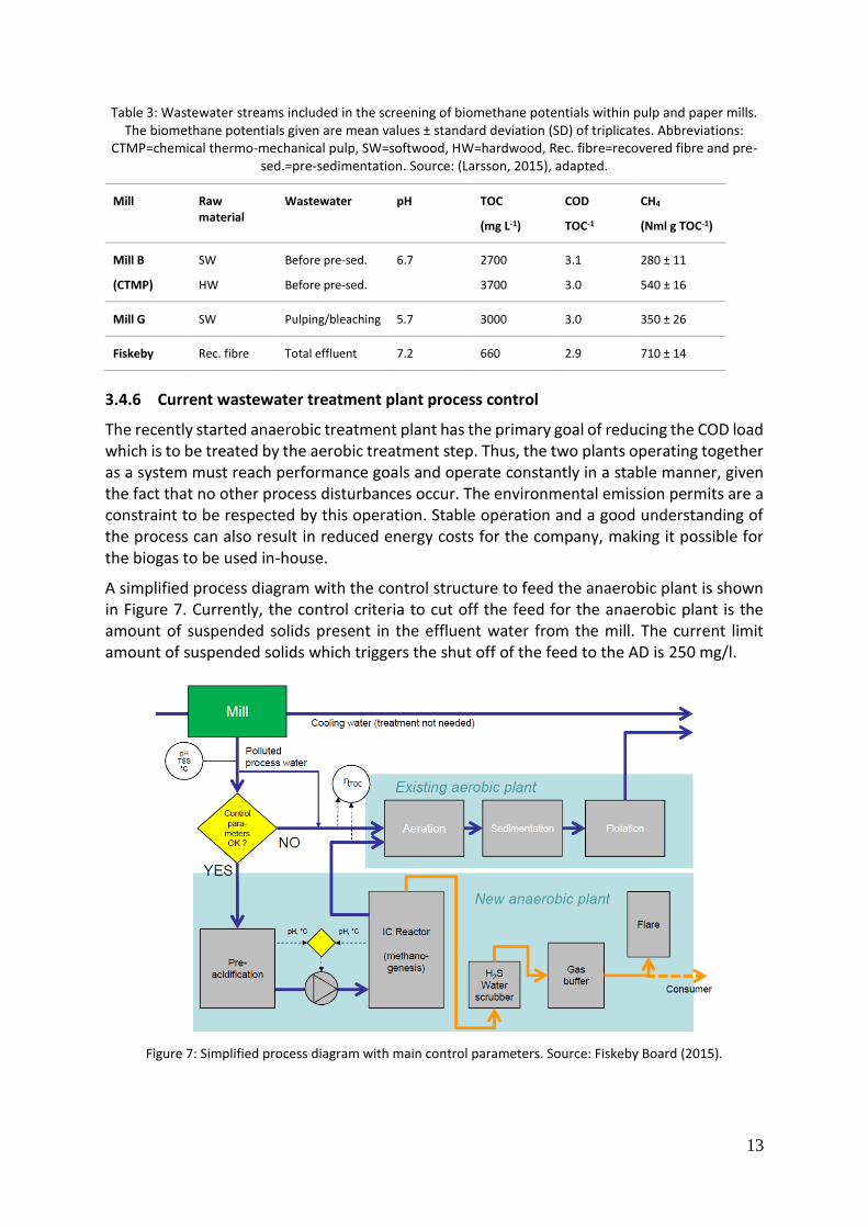
The biomethane potential of the wastewater from the board mill at Fiskeby was evaluated by Larsson (2015), together with the biomethane potential of the wastewaters of seven other pulp and paper mills. The analysis showed a biomethane production potential of 710 NmL CH4/g TOC, out of the maximum theoretical potential of 940 NmL CH4/g TOC. In fact, that was the highest biomethane potential found in this study. The analysis of the wastewater showed the presence of microscopic fragments of cellulose and a high content of dissolved starch, explaining its high biomethane potential. Selected results from three paper mills, including the wastewater from Fiskeby Board AB (identified as mill H), are shown in Table 3.
13
Table 3: Wastewater streams included in the screening of biomethane potentials within pulp and paper mills. The biomethane potentials given are mean values ± standard deviation (SD) of triplicates. Abbreviations:
CTMP=chemical thermo-mechanical pulp, SW=softwood, HW=hardwood, Rec. fibre=recovered fibre and pre-sed.=pre-sedimentation. Source: (Larsson, 2015), adapted.
Mill Raw material
Wastewater pH TOC
(mg L-1)
COD
TOC-1
CH4
(Nml g TOC-1)
Mill B
(CTMP)
SW
HW
Before pre-sed.
Before pre-sed.
6.7 2700
3700
3.1
3.0
280 ± 11
540 ± 16
Mill G SW Pulping/bleaching 5.7 3000 3.0 350 ± 26
Fiskeby Rec. fibre Total effluent 7.2 660 2.9 710 ± 14
3.4.6 Current wastewater treatment plant process control
The recently started anaerobic treatment plant has the primary goal of reducing the COD load which is to be treated by the aerobic treatment step. Thus, the two plants operating together as a system must reach performance goals and operate constantly in a stable manner, given the fact that no other process disturbances occur. The environmental emission permits are a constraint to be respected by this operation. Stable operation and a good understanding of the process can also result in reduced energy costs for the company, making it possible for the biogas to be used in-house.
A simplified process diagram with the control structure to feed the anaerobic plant is shown in Figure 7. Currently, the control criteria to cut off the feed for the anaerobic plant is the amount of suspended solids present in the effluent water from the mill. The current limit amount of suspended solids which triggers the shut off of the feed to the AD is 250 mg/l.
Figure 7: Simplified process diagram with main control parameters. Source: Fiskeby Board (2015).
14
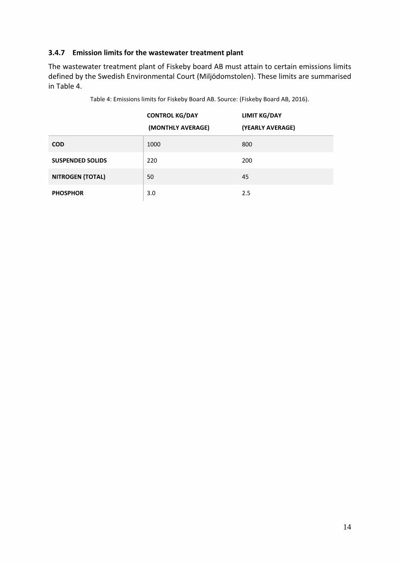
3.4.7 Emission limits for the wastewater treatment plant
The wastewater treatment plant of Fiskeby board AB must attain to certain emissions limits defined by the Swedish Environmental Court (Miljödomstolen). These limits are summarised in Table 4.
Table 4: Emissions limits for Fiskeby Board AB. Source: (Fiskeby Board AB, 2016).
CONTROL KG/DAY
(MONTHLY AVERAGE)
LIMIT KG/DAY
(YEARLY AVERAGE)
COD 1000 800
SUSPENDED SOLIDS 220 200
NITROGEN (TOTAL) 50 45
PHOSPHOR 3.0 2.5

15
4 Theory
4.1 Anaerobic process
The natural bacterial degradation of organic matter in anaerobic conditions releases methane (CH4), carbon dioxide (CO2) and traces of water (H2O), oxygen (O2), sulphur (S2) and hydrogen sulphide (H2S). This natural process is used under controlled conditions using biomass or organic load in wastewaters to produce biogas in industrial plants, varying from small to very large gas outputs. There are three categories of biomass which are used to produce biomethane in biogas plants (Wellinger, Murphy, & Baxter, 2013):
substrate from farms such as liquid manure, feed waste, harvest waste and energy
crops;
organic waste from households and municipalities such as food waste, market waste,
expired food and others;
industrial by-products such as glycerine, waste from food processing and fat
separators, industrial wastewaters.
In biogas plants, the organic matter is degraded in several steps in sealed digesters. The anaerobic bacterial process occurs in four steps: hydrolysis, acidification, production of acetic acid and, finally, production of methane. Depending on the substrate, the gas resulting from the bacterial degradation contains between 50 to 75% of methane, 25 to 50% carbon dioxide and trace materials as cited above (Wellinger et al., 2013). The biogas production involves a diverse group of microorganisms which have a greater degree of specialisation than those found in aerobic digestion and are exclusively anaerobic, all with specific requirements to allow their activation (Zinder, 1984).
The biogas production potential, and thus, the suitability of wastewaters to AD, depends highly in the characteristics of the substrate. These parameters are degradability of the organic material and the presence of inhibitory or toxic compounds (Larsson, 2015).
The degradability is a function of the ratio of easily degradable compounds, including cellulose, volatile fatty acids (VFAs) sugars, etc. An increased lignin content, on the other hand, tends to yield lower potentials.
The actual production process in the plant has additional processing steps which are required to guarantee an efficient operation and the highest possible gas yield. These steps vary according to the kind of substrate being used, as well as with the characteristics of the plant, which can use a dry or a wet digester process. The digesters are airtight tanks in which the substrate is introduced. The tanks can be vertical or horizontal, and generally they are mechanically mixed in a slow process to guarantee a residence time long enough for the bacteria to complete the digestion process. The temperature in the digesters is controlled and must be within certain limits. The process is called mesophilic if the temperature used is between 32 and 42 °C, and thermophilic if it is between 45 and 57 °C (Wellinger et al., 2013). The residence times tend to be shorter if thermophilic temperatures are used (Eder & Schulz, 2006). Additionally, other process controls are required, such as micronutrients for the bacteria and pH controls.
In the digester, biogas is produced and collected to be sent to the gas upgrading plant. The main function of the upgrading plant is to remove the CO2, dry the gas and remove the

16
contaminants such as hydrogen sulphide and sulphur. If the biogas is upgraded for a methane content of 98%, the result is often called biomethane and the product has the same properties as natural gas. For several applications, however, the upgrading process is not necessary, as the methane content of the biogas is high enough to be used directly by gas turbines or other equipment. In such cases, a desulphurisation step of the biogas production is sufficient to meet the requirements for usage.
4.1.1 Up flow anaerobic sludge bed (UASB) reactor
Up flow anaerobic sludge bed reactors are typically used for the treatment of wastewaters from different sources due to its lower retention time when compared to other reactor configurations (Eawag, 2014). Wastewater flows upwards, through the activated sludge and its organic content is degraded in the process. The biogas is collected by phase separators and the wastewater leaves at the top of the reactor. Typically, the reactor has a maturation period of up to three months (Tilley, Ulrich, Lüthi, Reymond, & Zurbrügg, 2014).
UASB reactors are sensitive to the sludge granules characteristics and are not suitable for wastewaters with large variations in organic load, and the minimum retention time should be of 2 hours, being typically of 4 to 20 hours. The advantages of such reactors are its lower cost of implementation, high rate of COD removal, low sludge production, direct use of the biogas production after scrubbing and relatively low space needed. The main disadvantages are the incapacity do deal with high fluctuations of the organic load, sensitiveness for the amount of suspended solids (10% of the COD load maximum), need for specialised operation and maintenance personnel and the requirement of further treatment of the wastewater downstream of the reactor. (Eawag, 2014), (Larsson, 2015)
A schematic view of a simple UASB reactor is shown in Figure 8.
Figure 8: UASB reactor schematic representation. Source: (Tilley et al., 2014).
4.2 Performance evaluation in biogas production
Performance evaluation in biogas production is a topic with much discussion in scientific literature. The criteria and performance indicators for biogas plants vary largely according to the type and objective of the installation. Other considerations regard the definition of system

17
boundaries, the definition of inputs and outputs to the plant and the consideration of energy inputs and outputs. Havukainen, Uusitalo, Niskanen, Kapustina, and Horttanainen (2014), performed a comprehensive study to evaluate methods that allow comparisons between different types of biogas installations, but with a focus on systems in which the energy and feedstocks inputs and outputs are defined to perform life cycle assessments. In the scope of this work, a more relevant set of indicators of performance relates to the composition of the wastewater and the energy use to achieve predefined parameters for the wastewater streams. In the following section, the relevant parameters for this study are defined.
4.2.1 Parameters and performance indicators
4.2.1.1 Volumetric loading rate
𝑉𝐿𝑅 = 𝐶𝑂𝐷𝑙𝑜𝑎𝑑
𝑉𝑟𝑒𝑎𝑡𝑜𝑟=
𝑄𝑖𝑛𝑓∗ 𝐶𝑂𝐷𝑖𝑛𝑓
𝑉𝑟𝑒𝑎𝑡𝑜𝑟 (1)
Where: VLR Volumetric loading rate (kg COD/m³. d)
Qinf Influent flow rate (m³/d)
CODload COD load to the reactor (kg/d)
CODinf COD concentration in the influent (kg/m³)
Vreactor Reactor volume (m³)
4.2.1.2 COD or BOD removal efficiency
𝜂𝐶𝑂𝐷 = 𝐶𝑂𝐷𝑖𝑛𝑓−𝐶𝑂𝐷𝑒𝑓𝑓
𝐶𝑂𝐷𝑖𝑛𝑓𝑥 100 (2)
Where: 𝜂𝐶𝑂𝐷 COD removal efficiency (%)
CODinf COD concentration in the influent (kg/m³)
CODeff COD concentration in the effluent (kg/m³)
Biochemical Oxygen Demand (BOD) can be replaced in the same calculation.
4.2.1.3 Specific biogas production
𝑆𝐺𝑃 = 𝑄𝑏𝑖𝑜𝑔𝑎𝑠
𝑄𝑖𝑛𝑓𝑥 𝐶𝑂𝐷𝑖𝑛𝑓 𝑥 𝜂𝐶𝑂𝐷
100 (3)
Where: SGP Specific biogas production (m³ biogas/ kg CODremoved)
𝑄𝑏𝑖𝑜𝑔𝑎𝑠 Biogas production (m³/d)
18
𝑄𝑖𝑛𝑓 Influent flow rate (m³/d)
CODinf COD concentration in the influent (kg/m³)
CODeff COD concentration in the effluent (kg/m³)
𝜂𝐶𝑂𝐷 COD removal efficiency (%)
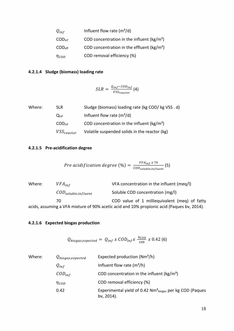
4.2.1.4 Sludge (biomass) loading rate
𝑆𝐿𝑅 = 𝑄𝑖𝑛𝑓∗ 𝐶𝑂𝐷𝑖𝑛𝑓
𝑉𝑆𝑆𝑟𝑒𝑎𝑐𝑡𝑜𝑟 (4)
Where: SLR Sludge (biomass) loading rate (kg COD/ kg VSS . d)
Qinf Influent flow rate (m³/d)
CODinf COD concentration in the influent (kg/m³)
𝑉𝑆𝑆𝑟𝑒𝑎𝑐𝑡𝑜𝑟 Volatile suspended solids in the reactor (kg)
4.2.1.5 Pre-acidification degree
𝑃𝑟𝑒 𝑎𝑐𝑖𝑑𝑖𝑓𝑖𝑐𝑎𝑡𝑖𝑜𝑛 𝑑𝑒𝑔𝑟𝑒𝑒 (%) = 𝑉𝐹𝐴𝑖𝑛𝑓 𝑥 70
𝐶𝑂𝐷𝑠𝑜𝑙𝑢𝑏𝑙𝑒,𝑖𝑛𝑓𝑙𝑢𝑒𝑛𝑡 (5)
Where: 𝑉𝐹𝐴𝑖𝑛𝑓 VFA concentration in the influent (meq/l)
𝐶𝑂𝐷𝑠𝑜𝑙𝑢𝑏𝑙𝑒,𝑖𝑛𝑓𝑙𝑢𝑒𝑛𝑡 Soluble COD concentration (mg/l)
70 COD value of 1 milliequivalent (meq) of fatty acids, assuming a VFA mixture of 90% acetic acid and 10% propionic acid (Paques bv, 2014).
4.2.1.6 Expected biogas production
𝑄𝑏𝑖𝑜𝑔𝑎𝑠,𝑒𝑥𝑝𝑒𝑐𝑡𝑒𝑑 = 𝑄𝑖𝑛𝑓 𝑥 𝐶𝑂𝐷𝑖𝑛𝑓𝑥 𝜂𝐶𝑂𝐷
100 𝑥 0.42 (6)
Where: 𝑄𝑏𝑖𝑜𝑔𝑎𝑠,𝑒𝑥𝑝𝑒𝑐𝑡𝑒𝑑 Expected production (Nm³/h)
𝑄𝑖𝑛𝑓 Influent flow rate (m³/h)
𝐶𝑂𝐷𝑖𝑛𝑓 COD concentration in the influent (kg/m³)
𝜂𝐶𝑂𝐷 COD removal efficiency (%)
0.42 Experimental yield of 0.42 Nm³biogas per kg COD (Paques bv, 2014).

19
4.2.1.7 Biomass sludge activity
𝐵𝑖𝑜𝑚𝑎𝑠𝑠 𝑠𝑙𝑢𝑑𝑔𝑒 𝑎𝑐𝑡𝑖𝑣𝑖𝑡𝑦 = 𝑄𝑖𝑛𝑓∗(𝐶𝑂𝐷𝑖𝑛𝑓−𝐶𝑂𝐷𝑒𝑓𝑓)
𝑉𝑆𝑆𝑟𝑒𝑎𝑐𝑡𝑜𝑟 (7)
Where: Biomass sludge activity (kg COD/ kg VSS . d)
𝑄𝑖𝑛𝑓 Influent flow rate (m³/d)
𝐶𝑂𝐷𝑖𝑛𝑓 COD concentration in the influent (kg/m³)
𝐶𝑂𝐷𝑒𝑓𝑓 COD concentration in the effluent(kg/m³)
𝑉𝑆𝑆𝑟𝑒𝑎𝑐𝑡𝑜𝑟 Volatile suspended solids in the reactor (kg)
20
5 Method
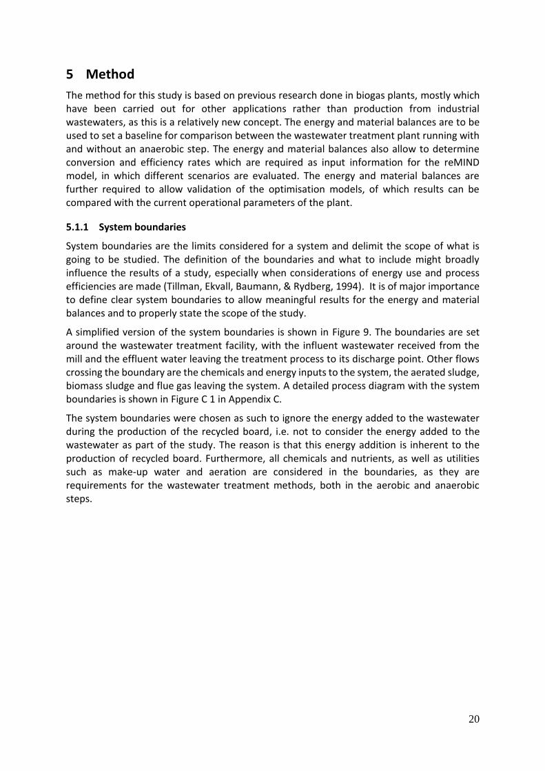
The method for this study is based on previous research done in biogas plants, mostly which have been carried out for other applications rather than production from industrial wastewaters, as this is a relatively new concept. The energy and material balances are to be used to set a baseline for comparison between the wastewater treatment plant running with and without an anaerobic step. The energy and material balances also allow to determine conversion and efficiency rates which are required as input information for the reMIND model, in which different scenarios are evaluated. The energy and material balances are further required to allow validation of the optimisation models, of which results can be compared with the current operational parameters of the plant.
5.1.1 System boundaries
System boundaries are the limits considered for a system and delimit the scope of what is going to be studied. The definition of the boundaries and what to include might broadly influence the results of a study, especially when considerations of energy use and process efficiencies are made (Tillman, Ekvall, Baumann, & Rydberg, 1994). It is of major importance to define clear system boundaries to allow meaningful results for the energy and material balances and to properly state the scope of the study.
A simplified version of the system boundaries is shown in Figure 9. The boundaries are set around the wastewater treatment facility, with the influent wastewater received from the mill and the effluent water leaving the treatment process to its discharge point. Other flows crossing the boundary are the chemicals and energy inputs to the system, the aerated sludge, biomass sludge and flue gas leaving the system. A detailed process diagram with the system boundaries is shown in Figure C 1 in Appendix C.
The system boundaries were chosen as such to ignore the energy added to the wastewater during the production of the recycled board, i.e. not to consider the energy added to the wastewater as part of the study. The reason is that this energy addition is inherent to the production of recycled board. Furthermore, all chemicals and nutrients, as well as utilities such as make-up water and aeration are considered in the boundaries, as they are requirements for the wastewater treatment methods, both in the aerobic and anaerobic steps.

21
Figure 9: Simplified process description with system boundaries
5.1.2 Unit processes
In order to detail the energy flows in the plant and construct the energy balance, it is required to break down the energy allocation to process steps.
Energy allocation in unit processes by end-use will be done according to Thollander (2014), and include whenever possible the following classification:
Space heating;
Space cooling;
Ventilation;
Tap hot water;
Lighting;
Compressed air;
Internal transport;
Pumping;
Administration;
Production processes.
For the current study, heating and cooling demands are not considered as the temperature in the anaerobic and aerobic processes is not actively controlled in the wastewater treatment plant. The wastewater comes from the board production machine with its temperature adjusted by heat exchangers for the wastewater treatment conditions within certain limits. Tap hot water, lighting, internal transport and administration energy uses are also neglected, as they are not exclusive for the wastewater treatment plant or not relevant. Under the classification of production processes of the wastewater treatment plant, a breakdown in more items is required to properly capture the steps of the treatment. These items are defined as follows:
Agitation

22
Aeration
Centrifuging
5.1.3 Data collection
The data collection relies on acquiring regularly recorded data from the plant and its sub processes, complemented by individual measurements if required and relevant. Data logged can be accessed through the control system of the plant and exported for analysis. In case a relevant energy or mass user in the plant is not currently covered by the plant’s control system, measurements assumptions based on process behaviour have to be made to estimate the required parameter.
Primarily, the measurements needed for the energy and material balances include:
Influents to the plant (flow, temperature, COD, total suspended solids (TSS), pH, chemical compounds);
Effluents of the plant: biogas, biomass, sludge (flow, temperature, COD, TSS, pH, etc.);
Electricity use by process equipment (kWh);
Aeration and ventilation requirements;
Consumption of chemicals, make-up water.
The plant’s control system allows the extraction of process parameters which are controlled online with a frequency of 8 seconds between measurements. Data is logged with a resolution of maximum five decimals places depending on the resolution of the correspondent sensor.
For the chemical composition of the wastewater, measurements with a frequency of 8 seconds are available for the influent and effluent water for total organic carbon (TOC) content and suspended solids, with laboratory analyses being done daily in samplers for intermediary steps of the plant. These samples provide daily averages and serve as quality control to the online system, but also to monitor different sections and to allow adjustments to the parameters.
The Swedish Standard (SS) 16231:2012 aims at providing a methodology to collect and analyse energy data in a way that allows comparison and the establishment of energy efficiency among and within entities. In this way, this standard offers an ideal framework for this project. The standard, however, is intended to address the general aspects of benchmarking (SIS, 2012a). As sector individual benchmarks are not in the scope of the standard, some adaptation is required for the current work and was done by dividing the production processes in the unit processes given in Section 5.1.2. Also, recommendations of the Swedish Standard SS EN16247-1:2012 for energy audits are taken into account (SIS, 2012b).
5.1.4 Recorded parameters
The SCADA system is the main source of data for this study. A total of 102 parameters related to the wastewater treatment plant, including the biogas plant, were accessed through a Microsoft Excel interface.
Due to a limitation in the number of cells that can be downloaded at once, the data for all parameters was imported for the period of 4 April 2015 to 1 May 2016. In this way, it was

23
possible to extract averages of each parameter for a period of 10 minutes between logs. When logs overlap in a given time period, the data is automatically interpolated to fit the timestamp of the parameter.
The complete list of parameters logged can be seen in Table E 1in Appendix E. The list includes the unit of the measurement, the description used in the plant, and minimum and maximum values considered for each parameter. The definition of such limits is necessary as it is common that sensors report measurements which are out of range and are not feasible for the parameter being measured. In such cases, parameters are ignored for the energy and material balances.
5.2 Energy and material balances
For the energy and material balances of the wastewater treatment plant, the different energy and material flows must be identified and measured. The measurements rely on data recorded historically in the plant and are complemented by measurements and surveys if no such data is available.
The balances are obtained after a survey of all flows crossing the system boundaries and all internal process steps and recirculation flows present in the plant. All electricity users are accounted for with different levels of detail according to their relevance and amount of data available, and this survey intends to correspond as close as possible to the actual energy and material uses and outputs in the plant.
Energy and material flows are allocated into unit processes relevant to the wastewater treatment plant under analysis, and the unit processes to be considered are based on Thollander (2014), with the necessary adaptations. The division in production and support processes when dividing the unit processes might not be relevant in such industrial system, and this is taken into consideration when classifying the unit process required for the study.
5.2.1 Calculations for the energy balance
For calculations required for the electrical motors in the plant which are not directly measured, calculations are done as an approximation depending on the flow which an electrical motor connected to a pump drives, and in typical motor efficiencies according to its rated power.
The electrical efficiency of a motor is relatively constant in the range of 50 to 100% of its rated power. The efficiency considered for motors without information available was estimated using the parameters in Figure 10. All motors are considered to be properly dimensioned to stay above 50% of its rated power at most times.
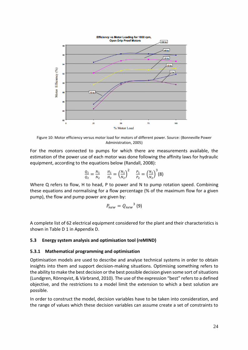
24
Figure 10: Motor efficiency versus motor load for motors of different power. Source: (Bonneville Power Administration, 2005)
For the motors connected to pumps for which there are measurements available, the estimation of the power use of each motor was done following the affinity laws for hydraulic equipment, according to the equations below (Randall, 2008):
𝑄1
𝑄2=
𝑁1
𝑁2
𝐻1
𝐻2= (
𝑁1
𝑁2)
2
𝑃1
𝑃2= (
𝑁1
𝑁2)
3
(8)
Where Q refers to flow, H to head, P to power and N to pump rotation speed. Combining these equations and normalising for a flow percentage (% of the maximum flow for a given pump), the flow and pump power are given by:
𝑃𝑛𝑒𝑤 = 𝑄𝑛𝑒𝑤3 (9)
A complete list of 62 electrical equipment considered for the plant and their characteristics is shown in Table D 1 in Appendix D.
5.3 Energy system analysis and optimisation tool (reMIND)
5.3.1 Mathematical programming and optimisation
Optimisation models are used to describe and analyse technical systems in order to obtain insights into them and support decision-making situations. Optimising something refers to the ability to make the best decision or the best possible decision given some sort of situations (Lundgren, Rönnqvist, & Värbrand, 2010). The use of the expression “best” refers to a defined objective, and the restrictions to a model limit the extension to which a best solution are possible.
In order to construct the model, decision variables have to be taken into consideration, and the range of values which these decision variables can assume create a set of constraints to

25
the model. The objective of the optimisation is defined trough an objective function that is composed by the decision variables.
In this context, mathematical programming refers to the computational mathematical methods and algorithms used to solve the mathematical expressions, relations and the sets of constraints present in an optimisation model.
The optimisation process includes the analysis of a real problem, the identification of the problem and its limitations, and most often its simplification. An optimisation model is then formulated based on the simplifications done, and an optimisation method is applied. The solution is thereafter studied against the real problem for evaluation and verification, and a final result is obtained.
The result is the set of values for the decision variables, which are both feasible and correspondent to the real problem.
An optimisation problem can be formulated as (Lundgren et al., 2010):
(𝑃) min𝑓(𝑥)
𝑠. 𝑡. 𝑥 ∈ 𝑋
Where f(x) is an objective function that depends on variables x = (x1, …,xn )T, and X defines feasible solutions to the problem, i.e. X is the set of constraints for the variables in x. The set of values of x which minimises f(x) is called an optimal solution to the problem.
5.3.2 reMIND
The Java-based energy system analysis and optimisation tool reMIND, which uses the MIND method (Method for analysis of INDustrial energy systems) is used to model and optimise the wastewater treatment plant, with special focus on the anaerobic digestion step. The MIND method was developed in-house at Linköping University and is based on Mixed Integer Linear Programming (MILP) (Karlsson, 2010).
In the reMIND model, the relevant sub steps of the wastewater treatment plant are modelled in order to evaluate optimisation opportunities in the plant. The model is then validated against the energy and material balances obtained, to check the consistency and limitations. After validation, if it is possible optimisation opportunities in different scenarios, including different criterion are performed. This can include cost reduction, biogas output, etc. Figure 11 shows a model of a paper and pulp mill using the reMIND software, as well as the program interface.

26
Figure 11: Model example of a pulp and paper mill using the reMIND software (Karlsson, 2010).
5.4 Literature review
Scientific research in Sweden is incipient in this kind of biogas production from wastewaters in pulp and paper mills. Often, the focus of already published research is on the chemical composition of the effluents and potential for treatment. This project focuses on energy issues and process interactions with the industrial process itself. The results from the reMIND model are used to allow comparison with similar plants found nationally and internationally, and information about such plants is to be found in a literature review. This includes information available in published research articles, when available, but also information from equipment suppliers and plant operators. The search for other studies is focused on works done in the last decade, as this is a new application of UASB reactors for the treatment of wastewaters in the pulp and paper industry. Keywords for the search include: “biogas plant efficiency”, “biogas production and potential in the pulp and paper industry”, “biogas potential from wastewaters in the pulp and paper industry”, and “biogas yield in industrial wastewaters”.
Such literature review is important not only to compare similar biogas facilities, but also to find out the advantages of such an installation in terms of energy and process benefits, as well as a validation for the use of the MIND method for this kind of analysis. Articles published in scientific journals and information made available by companies and operators are to be used.
27
6 Results and discussion
This section presents the results and analyses covering the objectives of this report. Section 6.2 presents two material balances for the wastewater treatment plant operation; one for the wastewater treatment plant before the commissioning of the biogas plant, and one for the operation with the biogas plant. Similarly, Section 6.3 presents two energy balances under the same criteria mentioned.
Section 6.6 presents the results for the reMIND models.
6.1 Initial considerations
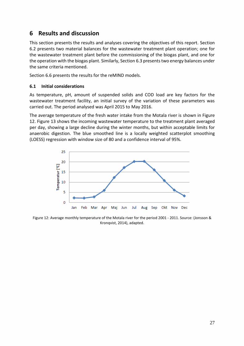
As temperature, pH, amount of suspended solids and COD load are key factors for the wastewater treatment facility, an initial survey of the variation of these parameters was carried out. The period analysed was April 2015 to May 2016.
The average temperature of the fresh water intake from the Motala river is shown in Figure 12. Figure 13 shows the incoming wastewater temperature to the treatment plant averaged per day, showing a large decline during the winter months, but within acceptable limits for anaerobic digestion. The blue smoothed line is a locally weighted scatterplot smoothing (LOESS) regression with window size of 80 and a confidence interval of 95%.
Figure 12: Average monthly temperature of the Motala river for the period 2001 - 2011. Source: (Jonsson & Kronqvist, 2014), adapted.

28
Figure 13: Daily average wastewater temperature inflow for the wastewater treatment plant. The green line indicates the start of the AD.
Figure 14 shows the incoming wastewater pH to the wastewater treatment plant, daily averaged. This variation is generally within the specification for AD, and the rise seen in August is not related to the introduction of the biogas plant, but rather by process variations in the board production machine and pulp preparation machines. However, the risen pH, to around 7.0 after the start of the biogas plant is beneficial to the AD process, as the acidification of the COD load in the reactor tends to lower the pH of the sludge bed. This way, the dosage of sodium hydroxide in the buffer tank is lowered.
Figure 14: Daily average of incoming wastewater pH. The green line indicates the start of the AD.
Figure 15 shows the amount of suspended solids in kg/day, daily averages. It is possible to see a growing trend in the period analysed, which is also related to the operational condition of the board machine and pulp preparation. Figure 16 shows the amount of suspended solids delivered back to the river in the same period, staying well below the emissions limit of 200 kg/day (yearly) for most days in the period. The peaks seen in the graph show moments when the biogas plant was stopped and the entire wastewater flow directed to the aeration basin directly, which resulted in a higher amount of suspended solids after the wastewater treatment plant. This is particularly true to the month of September, when frequent stops in

29
the AD reactor occurred due to operational issues related to the adaptation of the freshly added sludge to the plant’s conditions. On average, for the period before and after the start of the biogas plant, no significant changes in the concentration of suspended solids has occurred.
Figure 15: Suspended solids in the incoming wastewater. The green line indicates the start of the AD.
Figure 16: Suspended solids in the outflow of treated wastewater to the river. The green line indicates the start of the AD.
Figure 17 shows the total amount of TOC in kg/day for the incoming wastewater. TOC is the indirect measurement of the COD load of the wastewater used for online process control.

30
Figure 17: Total organic carbon in the incoming wastewater, daily values. The green line indicates the start of the AD.
6.2 Material and flow measurements
6.2.1 Before biogas commissioning
Table E 2 in Appendix E shows the calculation criteria for each flow considered for the plots. The calculation column in the table lists the Scada parameter used for each given flow and correlation factors determined for the measurements to be equivalent to the real flow observed in the plant. Such factors were obtained by studying the process and validating the data with process conditions and measurements done manually as controls to the online measurements. The period analysed for this balance is April to July 2015. Figure 18 to Figure 21 show all flows for each step of the wastewater treatment plant as the standard deviation of daily averages for a given week.
In Figure 18 it is possible to see a well behaved process for most weeks in the period, and how the dosage of chemicals and air, as well as the TOC and SS loads, vary together with the rate of inflow of wastewater to the plant.
Figure 19 once again shows that the dosage of chemicals is directly related to the flow of wastewater to the plant. It is also possible to see that the rate of recirculation of activated sludge is directly affected by the TOC load, and to the amount of SS in a less sensitive way. The amount of suspended solids in the overflow of the sedimentation does not appear to be directly related to the amount received by the plant or the rate in which activated sludge is returned to the aeration basin. For the centrifuge, in Figure 20 it is clear that the rate of removal of dried sludge is directly related to the amount of SS sent to this unit.
Finally, for the flotation step, in Figure 21, a higher amount of SS results in a higher flow of floated sludge being sent to the centrifuge, even at the relatively constant flow of wastewater treated in the unit, which indicates this step is efficient in accommodating the variations in SS received by the sedimentation basin.

31
Figure 18: Flows in the aeration basin for the wastewater treatment plant before biogas commissioning.
Figure 19: Flows in the sedimentation basin for the wastewater treatment plant before biogas commissioning.

32
Figure 20: Flows in the centrifuge for the wastewater treatment plant before biogas commissioning.
Figure 21: Flows in the flotation for the wastewater treatment plant before biogas commissioning.

33
6.2.2 After biogas commissioning
Table E 3 in Appendix E shows the calculation criteria for each flow considered for the plots. The procedure for the calculations is identical to the one described in section 6.2.1, with just the updates required to include the measurements from the AD step and the changes in the control system after the start-up of the biogas plant. The period analysed for this balance is August 2015 to April 2016. Figure 22 to Figure 26 show all flows for each step of the wastewater treatment plant as the standard deviation of daily averages for a given week.
Figure 22: Flows in the biogas plant for the wastewater treatment plant.
Figure 22 shows a direct correlation of the amount of biogas produced with the TOC load received by the biogas plant. Sodium hydroxide, used to regulate the pH of the wastewater was almost not used after stabilisation of the plant. The higher amount in the beginning is related to the rate of adaptation of the acidifying bacteria in the biomass, which has an adaptation time much shorter than the methanogenic culture. The urea dosed was reduced over time as well, the higher amount in the start of the series is related to the start-up, when a high dose of nitrogen is prescribed to allow bacterial adaptation. The feed of wastewater for the biogas plant has been varying over the period, which indicates that the plant is being bypassed frequently due to a too high concentration of SS in the influent. The increased dosed of phospor after the second week of 2016 has resulted in an increased biomass growth in the AD chamber, which is not shown in this graph as it is no measured bt the control system.

34
Figure 23: Flows in the aeration basin for the wastewater treatment plant.
In Figure 23 it is possible to see that the TOC and SS load in the aeration basin have a greater variation when compared to the period prior to the start-up of the biogas plant. This was expected to be seen, given that the biogas plant is not fed when the amount of suspended solids exceeds 250 mg/l. This has also led to an increased variation of the dosage of chemicals, but with smaller amounts being required as nutrients to the aerobic bacteria, as the COD load has been reduced. Such changes in the chemical dosing are discussed in section 6.4. One important flow to notice is the quantity of air pumped into the aeration, which has been decreasing over time as bacterial activity is reduced with the reduced COD load. The rate of return of activated sludge has varied much less since the introduction of the biogas plant.
Figure 24 shows a high amount of SS in the overflow of the sedimentation, probably related to the decay of bacteria after the TOC load to the aerobic treatment was reduced by the biogas plant. This decay process was observed for three weeks and is a result of the system adaptation to the new conditions. The rate of return of SS in the activated sludge has also seen a large decline. For the centrifuge, in Figure 25, the most important finding is the reduced amount of dried sludge, even though the flow of return sludge has not varied significantly compared to the previous period.
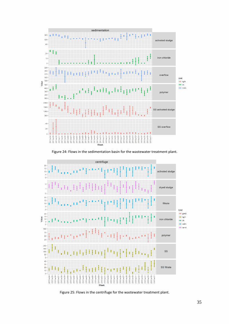
35
Figure 24: Flows in the sedimentation basin for the wastewater treatment plant.
Figure 25: Flows in the centrifuge for the wastewater treatment plant.

36
Figure 26: Flows in the flotation for the wastewater treatment plant.
Finally, for the flotation, in Figure 26 it can be seen that the amount of SS removed has not changed considerably in this unit with the start-up of the biogas plant, nor has the amount of SS and wastewater fed to the plant. However, the greater deviation seen in the feed of wastewater suggests that the unit can be bypassed more frequently.
6.3 Energy measurements
6.3.1 Before biogas commissioning
Table E 4 in Appendix E shows the calculation criteria for each equipment considered for the plots. For each equipment there is a power correction factor, based on the fact that most equipment does not operate at the rated power. For equipment which do not have a direct measurement available online and for which no detailed technical information was available, a factor of 0.9 was considered. Additionally, the runtime has been corrected based on estimations of operating time in proportion of the operating time of the treatment step where the equipment is installed. The calculation is then done based on the flow rate of pumps and blowers for which no direct measurement is available, using equation 9 from section 5.2.1. The period analysed for this balance is April to July 2015. Figure 27 shows the total energy use (kWh) per day, grouped by unit process in each process step. The “chemical” legend shows the pumping used for chemical dosage.

37
Figure 27: Total energy use (kWh) per day for each treatment step, grouped by unit process, before biogas commissioning.
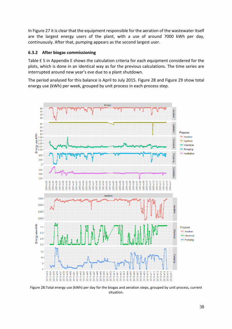
38
In Figure 27 it is clear that the equipment responsible for the aeration of the wastewater itself are the largest energy users of the plant, with a use of around 7000 kWh per day, continuously. After that, pumping appears as the second largest user.
6.3.2 After biogas commissioning
Table E 5 in Appendix E shows the calculation criteria for each equipment considered for the plots, which is done in an identical way as for the previous calculations. The time series are interrupted around new year’s eve due to a plant shutdown.
The period analysed for this balance is April to July 2015. Figure 28 and Figure 29 show total energy use (kWh) per week, grouped by unit process in each process step.
Figure 28:Total energy use (kWh) per day for the biogas and aeration steps, grouped by unit process, current situation.

39
Figure 29: Total energy use (kWh) per week for the sedimentation, centrifuge and flotation steps, grouped by unit process, current situation.
In Figure 28 it is possible to see that the biogas plant has been increasing its operational stability, which is demonstrated by the more stable energy use for pumping that feeds the reactor. In the aeration step from week 8, a considerable reduction in the energy use for aeration takes place. This is due to a test that the company is making to reduce the speed of the blowers automatically controlled by the concentration of oxigen in the aeration basin. This is now possible to be done as the COD load to the aerobic treatment is consistently

40
reduced by a stable operation of the biogas plant. Adittionally, the pumping of chemicals has largely reduced on all process steps. Figure 29 shows, in the other hand, that pumping in the flotation unit has increased slightly, but that is expected as the average flow of wastewater has increased.
6.4 Energy and material balances
Figure 30 presents the energy and mass balance for the plant operation prior to the commissioning of the biogas plant. Figure 31 shows the energy and mass balance for the current situation of the plant. The balance for the current installation was calculated using the measurements from January to April 2016. This was done to better capture the actual flows in the plant when it is running stably and under controlled conditions. The start-up of the plant involves larger dosage of chemicals and different control procedures to guarantee that the sludge inoculated to the reactor adapts to the conditions in the plant. This adaptation normally takes from two to four months (Mes, Stams, & Zeeman, 2003), thus performing the balance from January assures that the biological process is adapted to the influent characteristics.
Comparing both periods, the characteristics of the wastewater coming from the board mill are similar, but with a considerable decrease in the TOC load and PO4. Regarding the treated water leaving the plant, there was a slight increase in the amount of nitrogen and phosphor leaving the plant, which is probably related to the extra dosage of urea and phosphor in the AD reactor. As it can be seen, the amount of both compounds leaving the reactor are considerably higher than the incoming water. As these chemicals are nutrients for the aerobic sludge as well, the idea is to provide a higher amount for than necessary to the anaerobic bacteria and let the aerobic bacteria oxidise the extra load in the aerobic treatment. It might be necessary, however, to adjust these concentrations.
The amount of sludge dewatered in the centrifuge was lowered from 2 to 1.3 ton per day, which is congruent with the fact that most of the COD load passing through the AD is removed there. The volume of floated sludge in the flotation was also reduced, by 40.9%.
In the total water outlet to the river, the flow from the wastewater treatment plant is mixed with a flow of cooling water, which is just passed through the mill to remove heat from equipment. The control of emissions is done in this point of the factory, so the COD, SS, nitrogen and phosphor loads which are received from the river end up being summed up as part of the plant emissions, even though it is not a load emitted by the mill.
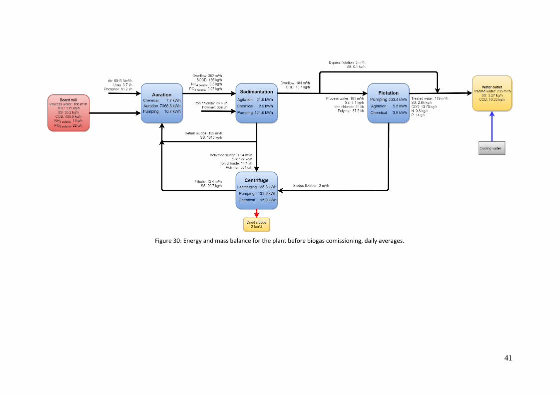
41
Figure 30: Energy and mass balance for the plant before biogas comissioning, daily averages.
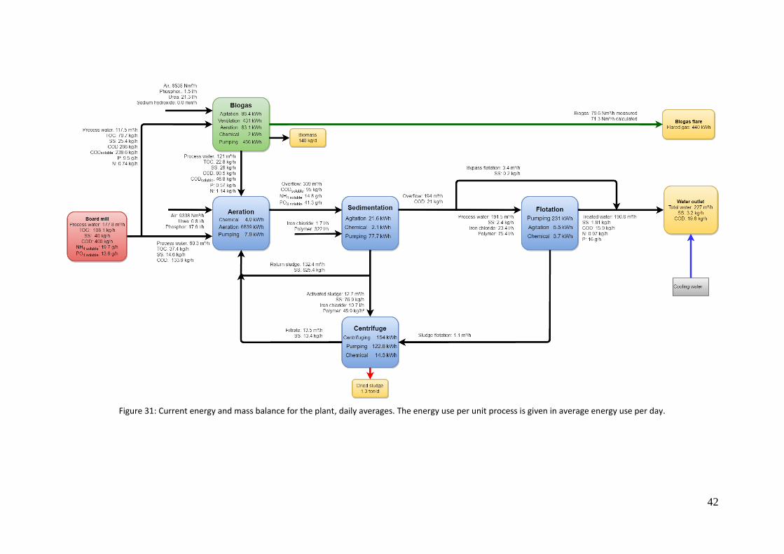
42
Figure 31: Current energy and mass balance for the plant, daily averages. The energy use per unit process is given in average energy use per day.

43
To allow direct comparison of the changes in the material flows, Table 5 presents values for both periods studied. Table 6 shows the correspondent information for energy use. Most of the equipment in the aerobic treatment showed a decrease in energy use, but the total energy use has increase by 9.4 % with the new equipment installed for the biogas plant.
Table 5: Average daily mass flows in the wastewater treatment plant for both periods analysed.
Mean SD Mean SD% difference
old/newUnit
Aeration Air 6915.0 659.0 9338.7 1207.2 35.7% Nm3/h
Aeration Urea 3.7 1.5 0.8 1.1 -76.5% l/h
Aeration Phosphor 61.2 35.8 17.6 30.7 -70.1% l/h
Aeration Process water 166.8 39.1 181.7 30.2 9.2% m3/h
Aeration TOC 121.0 44.0 37.4 36.6 -70.1% kg/h
Aeration SS 35.2 24.7 14.6 17.2 -59.6% kg/h
Aeration Activated sludge 155.3 17.5 132.4 20.8 -15.3% m3/h
Aeration Overflow aeration 335.5 45.9 326.8 38.3 -2.8% m3/h
Sedimentation Iron chloride 28.9 8.6 1.7 4.3 -94.5% l/h
Sedimentation Polymer 359.2 88.7 322.0 76.0 -10.0% l/h
Sedimentation Activated sludge 168.7 19.3 145.1 22.1 -14.7% m3/h
Sedimentation SS activated sludge 1613.1 438.4 902.3 467.4 -43.5% kg/h
Sedimentation SS overflow 4.2 4.7 3.1 2.9 -26.8% kg/h
Sedimentation Overflow 166.8 39.1 181.6 30.2 9.2% m3/h
Centrifuge Activated sludge 13.4 3.4 12.7 6.2 -7.9% m3/h
Centrifuge Iron chloride 14.1 4.7 10.7 5.9 -26.5% l/h
Centrifuge Polymer 60.0 21.4 45.9 16.1 -22.2% g/m3
Centrifuge SS 127.5 42.6 76.9 56.0 -40.5% kg/h
Centrifuge Filtrate 13.4 3.4 12.7 6.2 -7.8% m3/h
Centrifuge Dried sludge 2.0 0.8 1.3 1.1 -36.9% ton/d
Centrifuge SS filtrate 20.7 12.7 13.4 11.3 -36.3% kg/h
Flotation Process water 181.4 40.5 191.5 36.8 6.0% m3/h
Flotation SS 4.4 4.2 3.0 2.4 -31.2% kg/h
Flotation Iron chloride 25.1 13.1 23.4 9.2 -3.8% l/h
Flotation Polymer 87.5 29.9 75.4 27.9 -12.4% l/h
Flotation Treated water 179.4 40.2 190.6 36.5 6.6% m3/h
Flotation Floated sludge 2.0 1.9 1.1 1.2 -40.9% m3/h
Biogas Wastewater in 117.5 55.1 - m3/h
Biogas SS 25.4 11.8 - kg/h
Biogas TOC 70.7 35.6 - kg/h
Biogas Sodium hydroxide 0.0 0.0 - min
Biogas Air 6563.4 1129.4 - Nm3/h
Biogas Phosphor 1.5 0.9 - l/h
Biogas Urea 21.3 11.8 - l/h
Biogas Wastewater 122.3 55.8 - m3/h
Biogas Biogas calculated 71.3 30.9 - Nm3/h
Biogas Biogas measured 79.6 34.6 - Nm3/h
With biogas plant
From January 2016
-
Area Description
Without biogas
plant
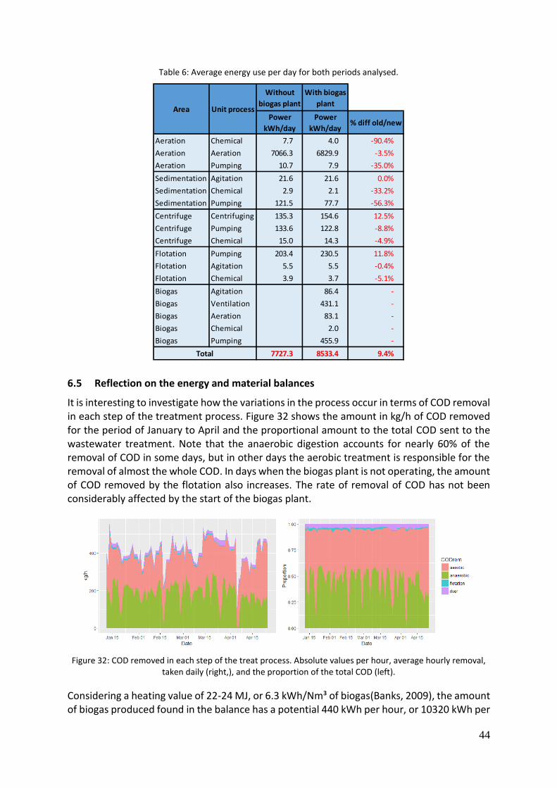
44
Table 6: Average energy use per day for both periods analysed.
6.5 Reflection on the energy and material balances
It is interesting to investigate how the variations in the process occur in terms of COD removal in each step of the treatment process. Figure 32 shows the amount in kg/h of COD removed for the period of January to April and the proportional amount to the total COD sent to the wastewater treatment. Note that the anaerobic digestion accounts for nearly 60% of the removal of COD in some days, but in other days the aerobic treatment is responsible for the removal of almost the whole COD. In days when the biogas plant is not operating, the amount of COD removed by the flotation also increases. The rate of removal of COD has not been considerably affected by the start of the biogas plant.
Figure 32: COD removed in each step of the treat process. Absolute values per hour, average hourly removal, taken daily (right,), and the proportion of the total COD (left).
Considering a heating value of 22-24 MJ, or 6.3 kWh/Nm³ of biogas(Banks, 2009), the amount of biogas produced found in the balance has a potential 440 kWh per hour, or 10320 kWh per
Without
biogas plant
With biogas
plant
Power
kWh/day
Power
kWh/day% diff old/new
Aeration Chemical 7.7 4.0 -90.4%
Aeration Aeration 7066.3 6829.9 -3.5%
Aeration Pumping 10.7 7.9 -35.0%
Sedimentation Agitation 21.6 21.6 0.0%
Sedimentation Chemical 2.9 2.1 -33.2%
Sedimentation Pumping 121.5 77.7 -56.3%
Centrifuge Centrifuging 135.3 154.6 12.5%
Centrifuge Pumping 133.6 122.8 -8.8%
Centrifuge Chemical 15.0 14.3 -4.9%
Flotation Pumping 203.4 230.5 11.8%
Flotation Agitation 5.5 5.5 -0.4%
Flotation Chemical 3.9 3.7 -5.1%
Biogas Agitation 86.4 -
Biogas Ventilation 431.1 -
Biogas Aeration 83.1 -
Biogas Chemical 2.0 -
Biogas Pumping 455.9 -
7727.3 8533.4 9.4%
Area Unit process
Total

45
daily, in average. This figure considers the calculated biogas production, not the measured one, as it is the lowest and most conservative of the two values. Considering a typical turbine with an efficiency of 35%, the amount of electricity produced if the biogas currently being flared was used would account to 3612 kW in power, which could supply 57 % of the current energy demand of the wastewater treatment plant. This would imply in a reduction in energy costs of approximately 3300 SEK/day.
The biogas potential of the wastewater was determined to be of 710 Nml/g.TOC-1 in the study of Larsson (2015). Equation (6) in chapter 4 determines the expected gas production based on experimental evidence (Paques bv, 2014). Figure 33 shows the comparison of the actual biogas production with these two estimations. Equation (6) yields similar results, whereas the biogas production is higher than the values found by Larsson (2015).
Figure 33: Expected gas production with COD removed versus actual production (up), and biogas potential by TOC removed versus actual production (down). The areas are coloured to show the overlap.
To investigate the amount of biogas lost because of the bypass of the anaerobic digestion due to the concentration of SS being above 250mg/l, the avoided biogas production in the period was analysed. In this period, the wastewater treatment plant operated for 2519 hours, and for 450 hours the wastewater feed for the anaerobic reactor was cut off due to the concentration of SS, which is 17.8% of the operation time. This resulted in an avoided TOC load to the reactor of 18.8 tons. The correlation between TOC and soluble COD is given in Table 7 in page 46. Based on this, the avoided biogas production adds up to 20360 Nm³, which corresponds to 10.2 % of the total volume of biogas produced in the period.
6.6 reMIND model
6.6.1 Input parameters
For the reMIND modelling, in order to reduce input parameters and set the node functions, correlations and efficiencies are defined in this section. As a simplification, the dosage of micronutrients for the bacteria and chemicals is assumed to be sufficient to not limit the
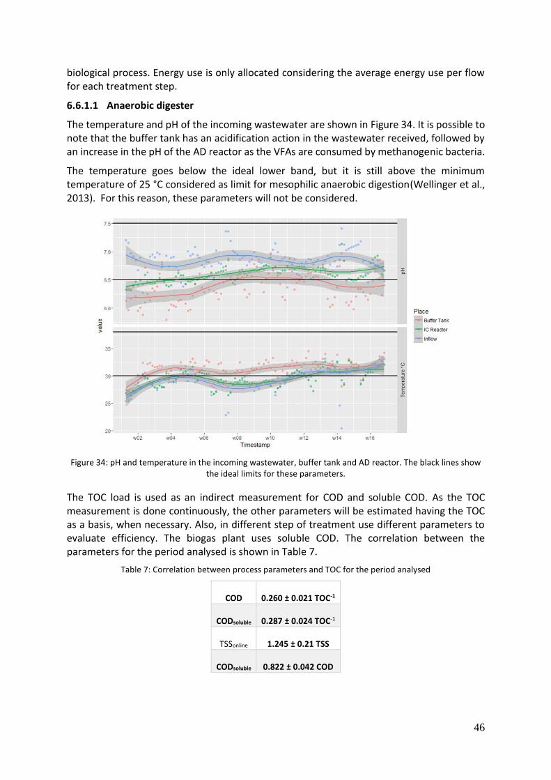
46
biological process. Energy use is only allocated considering the average energy use per flow for each treatment step.
6.6.1.1 Anaerobic digester
The temperature and pH of the incoming wastewater are shown in Figure 34. It is possible to note that the buffer tank has an acidification action in the wastewater received, followed by an increase in the pH of the AD reactor as the VFAs are consumed by methanogenic bacteria.
The temperature goes below the ideal lower band, but it is still above the minimum temperature of 25 °C considered as limit for mesophilic anaerobic digestion(Wellinger et al., 2013). For this reason, these parameters will not be considered.
Figure 34: pH and temperature in the incoming wastewater, buffer tank and AD reactor. The black lines show the ideal limits for these parameters.
The TOC load is used as an indirect measurement for COD and soluble COD. As the TOC measurement is done continuously, the other parameters will be estimated having the TOC as a basis, when necessary. Also, in different step of treatment use different parameters to evaluate efficiency. The biogas plant uses soluble COD. The correlation between the parameters for the period analysed is shown in Table 7.
Table 7: Correlation between process parameters and TOC for the period analysed
COD 0.260 ± 0.021 TOC-1
CODsoluble 0.287 ± 0.024 TOC-1
TSSonline 1.245 ± 0.21 TSS
CODsoluble 0.822 ± 0.042 COD

47
A correlation matrix for the main input and output parameters of the biogas plant is presented in Figure 35.
Figure 35: Pearson correlation matrix for parameters in the biogas reactor.
With this information, the selected parameters with relevance as inputs for the reMIND model are studied to see which correlations have significance. This is done additionally with the help of a grid of correlations and linear regression for each pair of considered parameters. Results are shown in Figure 36, in which the diagonal shows the density function of the points plotted, and the correlation value can be seen in the upper diagonal for each of the parameters.
Figure 36: Correlations in pair of parameters for inputs and outputs of the biogas plant. Diagonals are frequency distributions. Subscript “_ad” is a parameter leaving the plant.
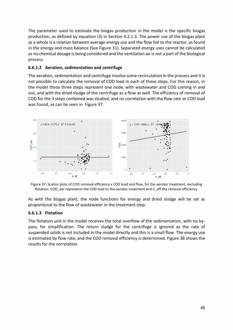
48
The parameter used to estimate the biogas production in the model is the specific biogas production, as defined by equation (3) in Section 4.2.1.3. The power use of the biogas plant as a whole is a relation between average energy use and the flow fed to the reactor, as found in the energy and mass balance (See Figure 31). Separated energy uses cannot be calculated as no chemical dosage is being considered and the ventilation air is not a part of the biological process.
6.6.1.2 Aeration, sedimentation and centrifuge
The aeration, sedimentation and centrifuge involve some recirculation in the process and it is not possible to calculate the removal of COD load in each of these steps. For this reason, in the model these three steps represent one node, with wastewater and COD coming in and out, and with the dried sludge of the centrifuge as a flow as well. The efficiency of removal of COD for the 3 steps combined was studied, and no correlation with the flow rate or COD load was found, as can be seen in Figure 37.
Figure 37: Scatter plots of COD removal efficiency x COD load and flow, for the aerobic treatment, excluding flotation. COD_aer represents the COD load to the aerobic treatment and n_eff the removal efficiency.
As with the biogas plant, the node functions for energy and dried sludge will be set as proportional to the flow of wastewater in the treatment step.
6.6.1.3 Flotation
The flotation unit in the model receives the total overflow of the sedimentation, with no by-pass, for simplification. The return sludge for the centrifuge is ignored as the rate of suspended solids is not included in the model directly and this is a small flow. The energy use is estimated by flow rate, and the COD removal efficiency is determined. Figure 38 shows the results for the correlation.

49
Figure 38: Correlation between efficienccy of flotation x COD load, flow. COD is the COD load to the flotation, n_eff the COD removal efficiency of this step.
With the information gathered in this section, the node parameters for the reMIND model are summarised in Table 8, as defined in Section 4.2.1.
Table 8: Input parameters for the reMIND model.
Area Parameter Value
Biogas
ηCOD (kg COD removed / kg COD
input)
0.692
SBP (m³ biogas/ kg COD removed) 0.346
ηBiomass (kg biomass/ kg COD
removed) 0.022
ηelectricity (kWh/ m³wastewater . h) 0.377
Aerobic treatment
ηCOD (kg COD removed / kg COD
input) 0.902
ηdried sludge (kg sludge/ kg COD
removed) 0.252
ηelectricity (kWh/ m³ wastewater . h) 1.66
Flotation
ηCOD (kg COD removed / kg COD
input) 0.256
ηelectricity (kWh/ m³ . h) 0.053

50
6.6.2 Built model
The model was built with the node parameters described in the previous section. It was then run for the baseline of the operation obtained in the energy and mass balance. The model built can be seen in Figure 39.
Figure 39: reMIND model for the wastewater treatment plant. Blue flows are wastewater, red COD load, black are dried aearated sludge from the centrifuge and anaerobic sludge from the AD reactor, respectively. Yellow
lines are electricity supply and green biogas produced. The node for the AD reactor includes the scrubber.
This model was run for a period of one day, in time steps of one hour. The constraints of the model are the process conditions given in the energy and material balance, as well as the operational limits of each process step. The results in comparison to the energy and material balance are shown in Table 9. Note that it was necessary to include dummy nodes between each node where a transfer of flow wastewater and COD occur. This happens because the optimisation model is not able to accommodate more than one resource flowing between two different nodes at a time. For this reason, the need of simplifications compromises the number of parameters that can be evaluated as serve as inputs to the model. Also, the variations in the process are highly dependent on the previous conditions of the plant, i.e., the degree of activation of the bacteria and proportion of organic loads received by each plant. This process is, additionally, very dynamic in time, so the long time steps tend to increase simulation errors.
Table 9:Validation of model results with the energy and mass balance obtained.
Parameter reMIND Energy/material balance
% difference
COD out, biogas (kg/h) 81.90 79.00 3.54%
COD out, aerobic (kg/h) 21.20 21.00 0.94%
COD out, flotation (kg/h) 15.77 15.90 -0.82%
Energy biogas (kWh) 44.10 44.44 -0.77%
Energy aerobic (kWh) 293.82 301.50 -2.61%
Energy flotation (kWh) 10.14 10.00 1.38%
Dried sludge (kg/h) 54.42 54.16 0.48%
Biomass (kg/h) 5.83 5.83 0.00%
Biogas (Nm3/h) 92.195 79.6 13.66%
51
The results of the model have small differences with the calculated balance, which is expected, as the optimisation was run with the same input conditions of the mass balance itself. For reMIND, the objective function aims at minimising the system costs. For the model, an energy price of 0.71 SEK/kWh, the average price for industry in Sweden (Eurostat, 2016). In this condition, the cost of electricity to run the plant for one day is 5 596 SEK. It is worth mentioning that the model had to be constrained to force the flow to the anaerobic digester. The reason for this is that the cost optimised solution tried to avoid the biogas plant all together, as it increases the energy use with the ‘extra’ treatment step.
To test the model with varying input conditions over days, seven different days of the period analysed were randomly selected among the days for which there are COD measurements in the flows needed.
In Table 10 (see page 52), the optimisation results are shown. It is clear that the optimisation using average correlation factors for especially the COD conversion rates in each step fails to predict these results with varying loads throughout the optimisation runs. For the flotation unit, particularly, the error is expected since the model cannot predict when the flotation step is running or not. The results are, however, acceptable for the energy use in each step, as the estimation is done in correlation with the flow, and that is a good prediction of the energy use of pumps. The biogas production, with an average error of 16.8 %, could also be considered acceptable for the optimisation parameters used.
The COD conversion rates did not show straight correlation in the analysis of the energy and material balances. As both the anaerobic and aerobic step are biological processes, the dynamics of such process affect the extent to which the model can evaluate how changes in these parameters influence the results. The other reason is the time step of the optimisation iterations, which has a broader span than required to capture the inherent biological dynamics of the process. It was not possible to reduce the time steps because the COD measurements in intermediary steps of the plant are daily averages and not constantly done. The correlation found for TOC – which has a constant online measurement available for the incoming wastewater – and COD is valid only for the influent of the biogas plant and the bypass of it. As conversion of organic matter takes place in the anaerobic and aerobic steps, the inorganic fraction of the COD increases and the correlation changes.

52
Table 10: Measurements for each day and simulation results. M_number identifies the measured value and S_number idenfies the simulation results.
M1 S1 M2 S2 M3 S3 M4 S4 M5 S5 M6 S6 M7 S7 mean error
COD out, biogas (kg/h) 110.8 81.9 50.3 60.5 102.5 112.3 87.9 85.2 82.3 80.8 64.1 68.8 44.0 46.0 -1.5% COD out, aerobic (kg/h) 24.9 46.2 24.7 32.6 23.7 50.1 22.7 40.4 19.8 40.4 22.0 49.9 17.7 42.2 -96.6% COD out, flotation (kg/h) 16.7 34.5 12.7 24.3 17.0 37.4 16.2 30.2 19.1 30.2 15.0 37.3 14.6 31.5 -103.9% Energy biogas (kWh) 1085.2 1293.7 1087.5 922.8 1094.4 1311.8 1081.3 1176.0 1062.0 1230.4 1020.0 741.9 968.9 533.8 3.4% Energy aerobic (kWh) 7111.7 6923.8 7317.9 6854.6 7487.4 6448.8 6879.2 5179.2 6547.0 5486.0 7728.6 7597.4 7764.5 8439.6 8.1% Energy flotation (kWh) 249.0 239.5 254.8 237.3 268.6 224.5 292.4 184.5 201.5 194.2 241.7 260.7 148.8 287.2 -4.7% Dried sludge (kg/h) 97.0 119.0 39.0 83.9 43.0 129.0 55.0 104.0 19.0 104.1 48.0 128.5 66.0 108.8 -158.2% Biomass (kg/h) 7.1 5.8 4.3 4.3 7.9 8.0 6.0 6.1 5.7 5.8 4.9 4.9 3.2 3.3 2.0% Biogas (Nm³/h) 86.0 79.3 60.0 58.6 101.0 108.6 79.0 82.4 114.0 78.2 122.0 66.6 77.0 44.5 16.8%
53
7 Conclusion
Energy and material balances were obtained for both the plant operating without the biogas plant, in the period of April to August 2015, for the treatment operating since start of the biogas reactor, from August 2015 to April 2016, and for the period after the stabilisation of the biomass sludge in the anaerobic reactor, from January to April 2016.
In the period of four months between the start of the biogas plant, from August to December 2015, the biomass sludge in the biogas reactor had time to adapt to the process conditions. It is known that anaerobic bacterial cultures have slower adaptation times than aerobics ones. This period also covered the learning and adaptation period for the plant personnel to the characteristics and operation requirements of anaerobic processes.
The energy balances obtained suggest that the operation of the plant is being stabilised as time passes, and that the introduction of the anaerobic treatment step resulted in benefits for the wastewater treatment plant. The amount of aerated sludge which is dried and removed from the aerobic step was reduced by 37%, the dosage of urea by 90%, phosphorus by 70%, iron chloride by 48% and polymers by 12%. This resulted as well in reduced energy uses for pumping of chemicals and recirculation feeds in the anaerobic step and the opportunity to reduce energy costs by the reduction of aeration flows in the aeration basin. The efficiency of the plant and biogas output is in accordance with expected values in the laboratory tests for the wastewater and the expected biogas production determined by the supplier of the equipment.
The reMIND optimisation tool showed to be adequate to understand energy uses in different process configurations, and to some extent to forecast the biogas production. The model, however, has limited capabilities regarding the prediction of parameters which are affected heavily by the biological conditions of the plant. The reason for this is both the number of required simplifications to implement the model, which requires conversion factors depending on correlations, and in which non-linear factors have difficult implementation.
The reMIND modelling, this was, is more suitable to be used in studies of steady process conditions, in situations where different permanent, or expected conditions, are to be considered. By allowing a good prediction of energy use and biogas output, the tool is adequate for feasibility studies such as the benefits of introducing an anaerobic step in a wastewater treatment plant. The model is particularly good in predicting energy use and how it varies in different conditions. To allow the modelling in reMIND to capture finer process variations, more information of parameters such as the TOC load leaving the AD reactor and each of the process steps would be required from the control system.
The fluctuations of parameters in the incoming wastewater to the treatment plant affect the dynamics of operation of the plant. The main disturbance found was the amount of suspended solids forcing the bypass of the anaerobic digester. This has occurred in 17.8% of the operation time of the plant and reduced the biogas output by 10%.
The variation in feed of COD load to the aerobic treatment directly has not resulted in lowered COD and chemical emissions after the flotation step. This suggests the anaerobic treatment has a limit to which it is capable of degrading the chemical oxygen demand, independent of the COD load, either because the biologically degradable COD has a concentration which is too low, or because most of the COD currently leaving the plant is not biologically degradable. The result of this is a stable COD output, indifferent of the COD load sent to the aerobic

54
treatment, given the limits of the plant. The aerobic treatment has a large buffer capacity within that limit, and can withhold stops in the anaerobic treatment. Additionally, the efficiency of removal of COD has not change considerably after the introduction of AD.
There is an opportunity to reduce the energy use of the aeration blowers – the highest installed power in the plant, and currently tests are being carried out to regulate the need for aeration with sensors of oxygenation in the aeration basin.

55
Future studies
Biogas production in wastewater streams from pulp and paper industry is somewhat new and tends to be implemented more commonly in the near future. To allow this process to speed up and provide technical background with supports efficient operations and reliable products, further research in anaerobic treatment in this industry sector is necessary.
Different pulp and paper mills use different production process which results in a variety of pollutants. The suitability of their wastewaters need to be assessed by complementary research, especially in regards of pilot plants which consider the specific dynamics of production of the pulp mills. The studies currently available evaluate biogas potential of only small fractions of the waste flows.
An energy and material balance was obtained in this study and the intention to compare the results with other biogas plants operating similarly has proven to be extremely difficult. There is no standard methodology to carry out such comparisons, and research on biogas production which proposes comparisons deals mostly with anaerobic digestion of food waste and manure. So, studies on methodologies to compare biogas plants, including those installed in industry, and, specifically, in pulp and paper industry, are required.
In the specific case study, there are several potential areas for future studies. When the biogas plant was first started, the idea was to reduce energy use for aeration in the aerobic step, but it was not possible to significantly reduce this use yet. This is related to the adaptation period of the aerobic bacteria, with the process of operational adaptation of the plant itself, and to the lack of information on how the introduction of anaerobic digestion could reduce aeration costs in combined wastewater treatment plants. This is an interesting line of study with a large potential to reduce energy use.
This project did not include the actual measurements of energy use for most of the plant equipment, but rather relied on indirect measurements of flows and the expected energy use which correlates to that. One way to improve the energy balances would be to directly measure the energy, and update the equations used in this project to the real observed runtime and operating conditions of each equipment. This way, the prediction of the use of energy would be more reliable.

56
References
Banks, C. (2009). Charles Banks. Retrieved from Southampton: http://www.forestry.gov.uk/pdf/rrps_AD250309_optimising_anaerobic_digestion.pdf/$FILE/rrps_AD250309_optimising_anaerobic_digestion.pdf
Bonneville Power Administration. (2005). A Guidebook for performing walk-through energy audits of industrial facilities (P. Christopher B. Milan, CEM Ed.).
Cipollone, V., & Zachmann, G. (2013, 9th October 2013). Empirics of energy competitiveness. Retrieved from http://zachmann.be/?p=627
Correljé, A., & van der Linde, C. (2006). Energy supply security and geopolitics: A European perspective. Energy Policy, 34(5), 532-543. doi:http://dx.doi.org/10.1016/j.enpol.2005.11.008
Eawag. (2014). UASB Reactor. Retrieved from http://www.sswm.info/category/implementation-tools/wastewater-treatment/hardware/semi-centralised-wastewater-treatments/u
Eder, B., & Schulz, B. (2006). Biogas Praxis – Grundlagen. Staufen bei Freiburg, Germany: ökobuch Verlag & Versand GmbH.
European Comission. (2014). Energy prices and costs in Europe. COMMUNICATION FROM THE COMMISSION TO THE EUROPEAN PARLIAMENT, THE COUNCIL, THE EUROPEAN ECONOMIC AND SOCIAL COMMITTEE AND THE COMMITTEE OF THE REGIONS COM(2014) 21 /2. Retrieved from Brussels: https://ec.europa.eu/energy/sites/ener/files/publication/Energy%20Prices%20and%20costs%20in%20Europe%20_en.pdf
European Parliament. (2009). Directive 2009/28/EC of the European Parliament and of the Council of 23 April 2009 on the promotion of the use of energy from renewable sources and amending and subsequently repealing Directives 2001/77/EC and 2003/30/EC. Retrieved from http://eur-lex.europa.eu/legal-content/EN/TXT/?uri=CELEX:32009L0028.
Europeiska miljöbyrån. (2004). Greenhouse gas emission trends and projections in Europe 2003 tracking progress by the EU and acceding and candidate countries towards achieving their Kyoto Protocol targets Environmental issue report, Retrieved from http://reports.eea.europa.eu/environmental_issue_report_2003_36/en/GHG_issue_36_FINAL_www.pdf
Eurostat. (2016). Energy price statistics - Eurostat statistics explained. Retrieved from http://ec.europa.eu/eurostat/statistics-explained/index.php/File:Electricity_and_gas_prices,_second_half_of_year,_2013%E2%80%9315_(EUR_per_kWh)_YB16.png
Fiskeby Board AB. (2016). This is Fiskeby. In F. B. AB (Ed.), (Vol. 2016, pp. Website).
Havukainen, J., Uusitalo, V., Niskanen, A., Kapustina, V., & Horttanainen, M. (2014). Evaluation of methods for estimating energy performance of biogas production. Renewable Energy, 66, 232-240. doi:http://dx.doi.org/10.1016/j.renene.2013.12.011

57
Hiller SP. (2016). Sludge Dewatering. Retrieved from http://hiller-us.com/sludge-dewatering.php
Jonsson, N., & Kronqvist, J. (2014). Utvärdering av kvalitén på vatten till anaerobt reningssteg vid kartongproducerande industri: Temperatur, mängd suspenderade ämnen samt flöden på Fiskeby Board AB. Retrieved from http://www.diva-portal.org/smash/get/diva2:731608/FULLTEXT01.pdf
Karlsson, M. (2010). The MIND method: A decision support for optmization of industrial energy systems - Principles and case studies. Applied Energy(88 (577-589)).
Larsson, M. (2015). Anaerobic Digestion of Wastewaters from Pulp and Paper Mills: A Substantial Source for Biomethane Production in Sweden. (Doctoral), Linköping University. Retrieved from http://liu.diva-portal.org/smash/record.jsf?pid=diva2:865661
Lundgren, J., Rönnqvist, M., & Värbrand, P. (2010). Optimization. Linköping: Studentlitteratur AB.
Magnusson, M., & Alvfors, P. (2012). Biogas potential in the Swedish pulp and paper industry. Paper presented at the International conference on clean energy 2012, Quebec, Canada, September 10-12 2012.
Mes, T. Z. D. d., Stams, A. J. M., & Zeeman, G. (2003). Methane production by anaerobic
digestion of wastewater and solid
wastes Biomethane and Biohydrogen. Status and perspectives of biological methane and hydrogen production. (pp. 102): Netherlands Agency for Energy and the Environment.
Meyer, T., & Edwards, E. A. (2014). Anaerobic digestion of pulp and paper mill wastewater and sludge. Water Research, 65, 321-349. doi:http://dx.doi.org/10.1016/j.watres.2014.07.022
Olsson, L., & Fallde, M. (2015). Waste(d) potential: a socio-technical analysis of biogas production and use in Sweden. Journal of Cleaner Production, 98, 107-115. doi:http://dx.doi.org/10.1016/j.jclepro.2014.02.015
Paques bv. (2014). Biopaq IC Reactor. Retrieved from
Paques bv. (2015). Tratamento de Gás e Geração de Biogás. Retrieved from http://br.paques.nl/produtos/featured/thiopaq-tratamento-de-gas-biogas
Randall, W. (2008). Basic Pump Parameters and the Affinity Laws.
SIS. (2012a). SVENSK STANDARD SS-EN 16231:2012: Energy efficiency benchmarking methodology. Stockholm, Sweden: SIS Förlag AB.
SIS. (2012b). SVENSK STANDARD SS-EN 16247-1-5:2012: Energy audits. Stockholm, Sweden: SIS Förlag AB.
Sustainable Development Platform. (2015). Sustainable Development Knowledge Platform. Retrieved from https://sustainabledevelopment.un.org/sdg7
Sveriges Riksdag. (2013). Industriutsläppsförordning (2013:250). Retrieved from http://www.riksdagen.se/sv/dokument-lagar/dokument/svensk-forfattningssamling/industriutslappsforordning-2013250_sfs-2013-250.
58
Swedish Energy Agency. (2015). Energy in Sweden 2015. Retrieved from https://www.energimyndigheten.se/globalassets/statistik/overgripande-rapporter/energy-in-sweden-till-webben.pdf
Swedish Forest Industries Federation. (2015). Facts and Figures 2014. Retrieved from http://www.forestindustries.se/MediaBinaryLoader.axd?MediaArchive_FileID=4e041c87-0147-4f43-9b13-3a2122d9aaf0&FileName=Facts+and+figures+2014.pdf
The Environmental Paper Network. (2015). The State of the Paper Industry: Monitoring the Indicators of Environmental Performance. Retrieved from http://www.greenpressinitiative.org/documents/StateOfPaperInd.pdf
Thollander, P. (2008). Towards Increased Energy Efficiency in Swedish Industry Barriers, Driving Forces and Policies. Linköping: Linköping University Electronic Press.
Thollander, P. (2014). Data categorization 2014-11-05. Retrieved from
Tilley, E., Ulrich, L., Lüthi, C., Reymond, P., & Zurbrügg, C. (2014). Compendium of Sanitation Systems and Technologies (2nd ed.). Duebendorf, Switzerland: Swiss Federal Institute of Aquatic Science and Technology (Eawag).
Tillman, A.-M., Ekvall, T., Baumann, H., & Rydberg, T. (1994). Choice of system boundaries in life cycle assessment. Journal of Cleaner Production, 2(1), 21-29. doi:http://dx.doi.org/10.1016/0959-6526(94)90021-3
Kyoto Protocol to the United Nations Framework Convention on Climate Change adopted at COP3, (1997).
Wellinger, A., Murphy, J., & Baxter, D. (2013). The biogas handbook. Science, production and applications. Cambridge: Woodhead Publishing Limited.
Zinder, S. (1984). Microbiology of anaerobic conversion of organic wastes to methane: recent developments. Am. Soc. Microbiol. News;(United States), 50(7).

59
Appendices
Appendix A
Figure A 1: Process flowchart with individal flows and equipment
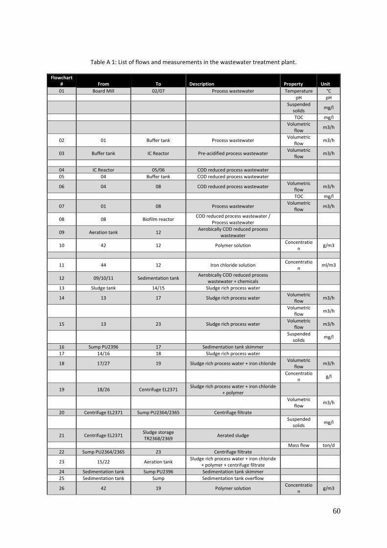
60
Table A 1: List of flows and measurements in the wastewater treatment plant.
Flowchart # From To Description Property Unit
01 Board Mill 02/07 Process wastewater Temperature °C
pH pH
Suspended
solids mg/l
TOC mg/l
Volumetric
flow m3/h
02 01 Buffer tank Process wastewater Volumetric
flow m3/h
03 Buffer tank IC Reactor Pre-acidified process wastewater Volumetric
flow m3/h
04 IC Reactor 05/06 COD reduced process wastewater
05 04 Buffer tank COD reduced process wastewater
06 04 08 COD reduced process wastewater Volumetric
flow m3/h
TOC mg/l
07 01 08 Process wastewater Volumetric
flow m3/h
08 08 Biofilm reactor COD reduced process wastewater /
Process wastewater
09 Aeration tank 12 Aerobically COD reduced process
wastewater
10 42 12 Polymer solution Concentratio
n g/m3
11 44 12 Iron chloride solution Concentratio
n ml/m3
12 09/10/11 Sedimentation tank Aerobically COD reduced process
wastewater + chemicals
13 Sludge tank 14/15 Sludge rich process water
14 13 17 Sludge rich process water Volumetric
flow m3/h
Volumetric
flow m3/h
15 13 23 Sludge rich process water Volumetric
flow m3/h
Suspended
solids mg/l
16 Sump PU2396 17 Sedimentation tank skimmer
17 14/16 18 Sludge rich process water
18 17/27 19 Sludge rich process water + iron chloride Volumetric
flow m3/h
Concentratio
n g/l
19 18/26 Centrifuge EL2371 Sludge rich process water + iron chloride
+ polymer
Volumetric
flow m3/h
20 Centrifuge EL2371 Sump PU2364/2365 Centrifuge filtrate
Suspended
solids mg/l
21 Centrifuge EL2371 Sludge storage TR2368/2369
Aerated sludge
Mass flow ton/d
22 Sump PU2364/2365 23 Centrifuge filtrate
23 15/22 Aeration tank Sludge rich process water + iron chloride
+ polymer + centrifuge filtrate
24 Sedimentation tank Sump PU2396 Sedimentation tank skimmer
25 Sedimentation tank Sump Sedimentation tank overflow
26 42 19 Polymer solution Concentratio
n g/m3

61
27 44 18 Iron chloride solution Concentratio
n kg/ton
28 Phosphorous tank 29/30 Phosphorous solution Volumetric
flow l/h
29 28 23 Phosphorous solution Volumetric
flow l/h
30 28 Aeration tank Phosphorous solution Volumetric
flow l/h
31 Urea tank Aeration tank Urea solution Volumetric
flow l/h
32 Water grid Biofilm reactor Make-up water for antifoaming spray
nozzles
33 PU2372 Biofilm reactor Aeration air Pressure mbar
34 PU2356 36 Aeration air
35 PU2997 36 Aeration air
36 34/35 Aeration tank Aeration air Pressure mbar
Volumetric
flow Nm3/h
37 EL3174 Hyperdive Aeration air
38 Buffer tank 40 Ventilation air Volumetric
flow Nm3/h
39 IC Reactor 40 Ventilation air Volumetric
flow Nm3/h
40 38/39 Aeration tank Ventilation air Volumetric
flow Nm3/h
Pressure mbar
41 42 Flotation Polymer solution Volumetric
flow l/h
Concentratio
n ml/m3
42 Polymer tank 10/26/41 Polymer solution Volumetric
flow l/h
43 44 Flotation Iron chloride solution Volumetric
flow l/h
44 Iron chloride tank 27/43 Iron chloride solution
45 Sump Flotation Sedimentation overflow Suspended
solids mg/l
46 Flotation 17 Flotation overflow Volumetric
flow m3/h
47 Sump 51 Sump overflow / Treated wastewater
48 Flotation 49 Flotation underflow
49 48 51 Flotation underflow
50 48 Aeration system
Flotation Flotation underflow
51 47/49 Recipient tank Board
Mill Treated wastewater
Suspended solids
mg/l
52 Urea tank Buffer tank Urea solution Concentratio
n g/m3
Volumetric
flow l/h
53 Phosphorous tank Buffer tank Phosphorous solution Concentratio
n g/m3
Volumetric
flow l/h
54 NaOH tank 55/56 NaOH solution
55 54 Buffer tank NaOH solution
56 54 Bioreactor Thiopaq NaOH solution
57 Nutrient tank Bioreactor Thiopaq Nutrient solution
58 K601 Bioreactor Thiopaq Aeration air
59 Gas scrubber Bioreactor Thiopaq Sulphur rich solution
60 Bioreactor Thiopaq 60/67 Bioreactor water
61 60 Sedimentation
Thiopaq Bioreactor water
62 Sedimentation
Thiopaq Bioreactor Thiopaq Sulphur poor solution
63 Sedimentation
Thiopaq Aeration tank Elementary sulphur sludge

62
64 IC Reactor 65 Sulphur rich biogas Volumetric
flow Nm3/h
Pressure mbar
65 64 Gas scrubber Sulphur rich biogas
66 Condensate tank Buffer tank Condensate
67 60 Gas scrubber Bioreactor water
68 Gas scrubber Biogas buffer Sulphur poor biogas Volumetric
flow Nm3/h
69 Condensate tank Buffer tank Condensate
70 Biogas buffer Flare Sulphur poor biogas
71 Compressed air ring Aeration system
Flotation Compressed air
72 Aeration system
Flotation Aeration column
Flotation Compressed air + water
73 Water grid Bioreactor Thiopaq Make-up water for Thiopaq Pressure bar
74 IC Reactor Biomass outlet Biomass sludge
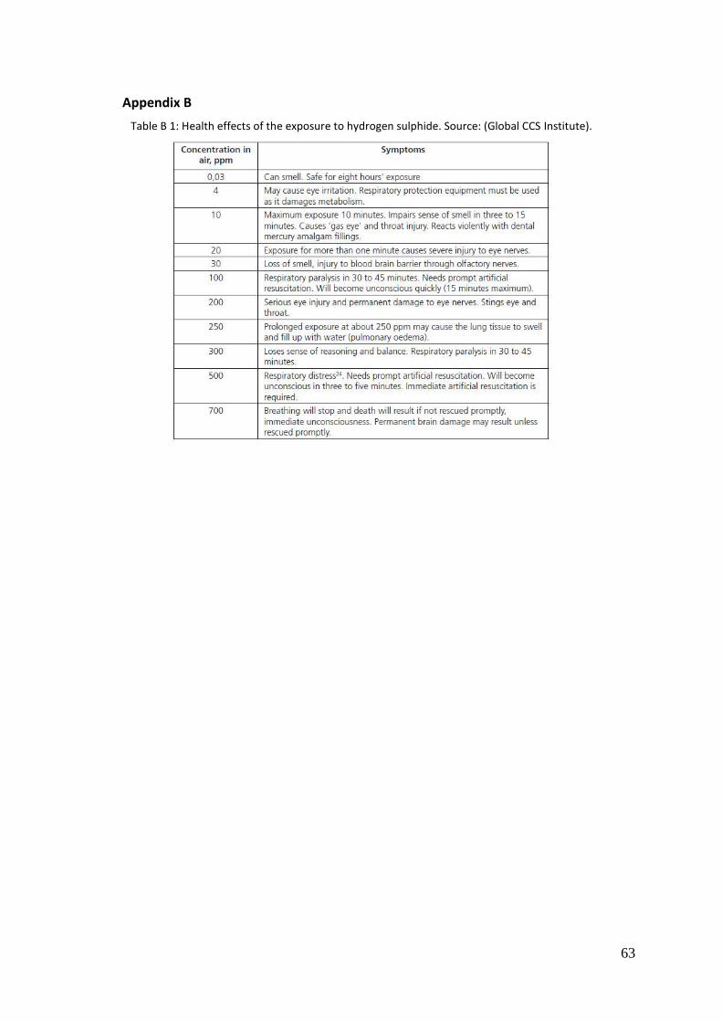
63
Appendix B
Table B 1: Health effects of the exposure to hydrogen sulphide. Source: (Global CCS Institute).

64
Appendix C
Figure C 1: Process diagram for the wastewater treatment plant with system boundaries.
.
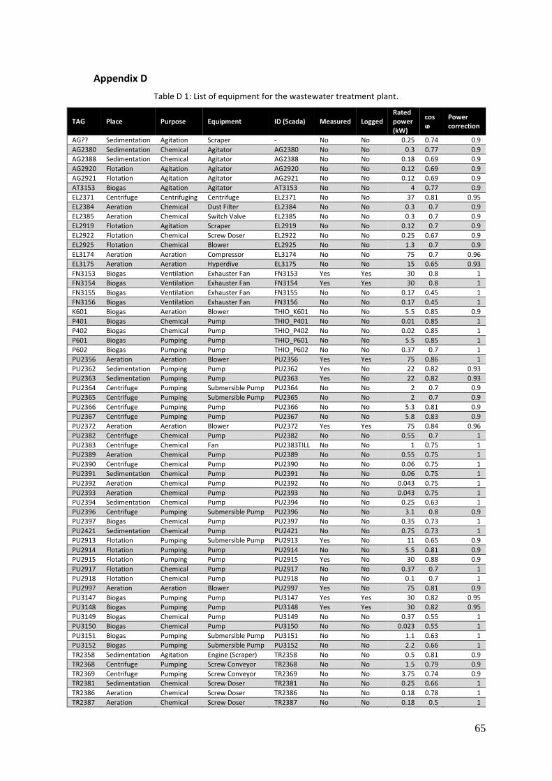
65
Appendix D
Table D 1: List of equipment for the wastewater treatment plant.
TAG Place Purpose Equipment ID (Scada) Measured Logged Rated power (kW)
cos ⱷ
Power correction
AG?? Sedimentation Agitation Scraper - No No 0.25 0.74 0.9
AG2380 Sedimentation Chemical Agitator AG2380 No No 0.3 0.77 0.9
AG2388 Sedimentation Chemical Agitator AG2388 No No 0.18 0.69 0.9
AG2920 Flotation Agitation Agitator AG2920 No No 0.12 0.69 0.9
AG2921 Flotation Agitation Agitator AG2921 No No 0.12 0.69 0.9
AT3153 Biogas Agitation Agitator AT3153 No No 4 0.77 0.9
EL2371 Centrifuge Centrifuging Centrifuge EL2371 No No 37 0.81 0.95
EL2384 Aeration Chemical Dust Filter EL2384 No No 0.3 0.7 0.9
EL2385 Aeration Chemical Switch Valve EL2385 No No 0.3 0.7 0.9
EL2919 Flotation Agitation Scraper EL2919 No No 0.12 0.7 0.9
EL2922 Flotation Chemical Screw Doser EL2922 No No 0.25 0.67 0.9
EL2925 Flotation Chemical Blower EL2925 No No 1.3 0.7 0.9
EL3174 Aeration Aeration Compressor EL3174 No No 75 0.7 0.96
EL3175 Aeration Aeration Hyperdive EL3175 No No 15 0.65 0.93
FN3153 Biogas Ventilation Exhauster Fan FN3153 Yes Yes 30 0.8 1
FN3154 Biogas Ventilation Exhauster Fan FN3154 Yes Yes 30 0.8 1
FN3155 Biogas Ventilation Exhauster Fan FN3155 No No 0.17 0.45 1
FN3156 Biogas Ventilation Exhauster Fan FN3156 No No 0.17 0.45 1
K601 Biogas Aeration Blower THIO_K601 No No 5.5 0.85 0.9
P401 Biogas Chemical Pump THIO_P401 No No 0.01 0.85 1
P402 Biogas Chemical Pump THIO_P402 No No 0.02 0.85 1
P601 Biogas Pumping Pump THIO_P601 No No 5.5 0.85 1
P602 Biogas Pumping Pump THIO_P602 No No 0.37 0.7 1
PU2356 Aeration Aeration Blower PU2356 Yes Yes 75 0.86 1
PU2362 Sedimentation Pumping Pump PU2362 Yes No 22 0.82 0.93
PU2363 Sedimentation Pumping Pump PU2363 Yes No 22 0.82 0.93
PU2364 Centrifuge Pumping Submersible Pump PU2364 No No 2 0.7 0.9
PU2365 Centrifuge Pumping Submersible Pump PU2365 No No 2 0.7 0.9
PU2366 Centrifuge Pumping Pump PU2366 No No 5.3 0.81 0.9
PU2367 Centrifuge Pumping Pump PU2367 No No 5.8 0.83 0.9
PU2372 Aeration Aeration Blower PU2372 Yes Yes 75 0.84 0.96
PU2382 Centrifuge Chemical Pump PU2382 No No 0.55 0.7 1
PU2383 Centrifuge Chemical Fan PU2383TILL No No 1 0.75 1
PU2389 Aeration Chemical Pump PU2389 No No 0.55 0.75 1
PU2390 Centrifuge Chemical Pump PU2390 No No 0.06 0.75 1
PU2391 Sedimentation Chemical Pump PU2391 No No 0.06 0.75 1
PU2392 Aeration Chemical Pump PU2392 No No 0.043 0.75 1
PU2393 Aeration Chemical Pump PU2393 No No 0.043 0.75 1
PU2394 Sedimentation Chemical Pump PU2394 No No 0.25 0.63 1
PU2396 Centrifuge Pumping Submersible Pump PU2396 No No 3.1 0.8 0.9
PU2397 Biogas Chemical Pump PU2397 No No 0.35 0.73 1
PU2421 Sedimentation Chemical Pump PU2421 No No 0.75 0.73 1
PU2913 Flotation Pumping Submersible Pump PU2913 Yes No 11 0.65 0.9
PU2914 Flotation Pumping Pump PU2914 No No 5.5 0.81 0.9
PU2915 Flotation Pumping Pump PU2915 Yes No 30 0.88 0.9
PU2917 Flotation Chemical Pump PU2917 No No 0.37 0.7 1
PU2918 Flotation Chemical Pump PU2918 No No 0.1 0.7 1
PU2997 Aeration Aeration Blower PU2997 Yes No 75 0.81 0.9
PU3147 Biogas Pumping Pump PU3147 Yes Yes 30 0.82 0.95
PU3148 Biogas Pumping Pump PU3148 Yes Yes 30 0.82 0.95
PU3149 Biogas Chemical Pump PU3149 No No 0.37 0.55 1
PU3150 Biogas Chemical Pump PU3150 No No 0.023 0.55 1
PU3151 Biogas Pumping Submersible Pump PU3151 No No 1.1 0.63 1
PU3152 Biogas Pumping Submersible Pump PU3152 No No 2.2 0.66 1
TR2358 Sedimentation Agitation Engine (Scraper) TR2358 No No 0.5 0.81 0.9
TR2368 Centrifuge Pumping Screw Conveyor TR2368 No No 1.5 0.79 0.9
TR2369 Centrifuge Pumping Screw Conveyor TR2369 No No 3.75 0.74 0.9
TR2381 Sedimentation Chemical Screw Doser TR2381 No No 0.25 0.66 1
TR2386 Aeration Chemical Screw Doser TR2386 No No 0.18 0.78 1
TR2387 Aeration Chemical Screw Doser TR2387 No No 0.18 0.5 1

66
Appendix E
Table E 1: List of parameters obtained from the Scada system.
Scada ID Unit Description SCADA Min Max Area Direction
Q-044MV mg/l GRUMLIGHET HUVUDAVL. 0 320 Flotation Output
Q-1175MV mg/l Susp.halt 3:e steget 0 500 Flotation Input
L-976MV m SLAMNIVÅ SED.BASSÄNG 0 10 Sedimentation Internal
F-835 g/m3 POLYMER BASSÄNG 0 12 Sedimentation Input
F-835MV l/h POLYMER TILL BASSÄNG 0 540 Sedimentation Input
F-832 ml/m3 FENNOFLOCK F111 0 300 Sedimentation Input
F-832MV l/h FENNOFLOCK F111 0 50 Sedimentation Input
F-975 m3/h FLÖDE SLAMRETUR 0 250 Aeration Input
F-649 kg/ton JÄRNKLORID CENTRIFUG 0 250 Centrifuge Input
F-649MV l/h JÄRNKLORID CENTRIFUG 0 35 Centrifuge Input
F-834MV m3/h FLÖDE ÖVERSK.SLAMMA 0 26 Centrifuge Input
F-834MVCV3 ton/d FLÖDE TILL SLAMFLAK 0 6 Centrifuge Output
F-836MVCV g/m3 POLYMER CENTRIFUG 0 120 Centrifuge Input
P-1311MV mbar BLÅSLUFT SELEKTORB. 0 750 Aeration Input
P-1312MV mbar BLÅSLUFT LUFTN.BAS 0 800 Aeration Input
Q-746 mg/l SYREHALT LUFTNINGSB. 0 20 Aeration Internal
F-1388MV Nm3/h FLÖDE BLÅSLUFT 0 6000 Aeration Input
Q-745 mg/l SYREHALT BIOSTEG 0 10 Aeration Internal
Q-741MV pH pH TILL AKT.SLAMANL. 0 14 Aeration Internal
T-740 oC TEMP TILL VATTENREN. 0 60 Aeration Internal
F-743 m3/h FLÖDE TILL AKT.SLAM 0 350 Aeration Internal
Q-873 mg/l SUSP.HALT EFT.MERI 0 2005 Aeration Internal
F-831 l/h FOSFORSYRA BASSÄNG 0 10 Aeration Input
F-833 l/h UREA BASSÄNG 0 200 Aeration Input
L-747MV1 % PUMPGROP FLYTSLAM 0 110 Centrifuge Internal
L-747MV2 % PUMPGROP CENTRIFUG 0 110 Aeration Input
G-1309VARVTID min VARVTID SLAMSKRAPA 0 365 Sedimentation Internal
F-1401 m3/h FLÖDE T BUFFERTTANK 0 260 Biogas Input
F-1402 m3/h FLÖDE T AKTIVT SLAM 0 335 Aeration Input
Q-741MVCV pH pH EFTER VVX KM1 0 14 Biogas Input
Q-1398MVCV mg/l SUSP EFTER VVX KM1 0 1000 Biogas Input
Q-1323MV mg/l TOC INK. VATTEN 0 2000 Biogas Input
Q-1405SP pH 0 14 Biogas Internal
Q-1405MV pH pH BUFFERTTANK 0 14 Biogas Internal
T-1404MV oC TEMP BUFFERTTANK 0 60 Biogas Internal
F-1408 m3/h FLÖDE TILL REAKTOR 0 265 Biogas Internal
Q-1410MV pH pH IC-REAKTOR 0 14 Biogas Internal
T-1409MV oC TEMP IC-REAKTOR 0 60 Biogas Internal
L-1415 % NIVÅ UTLOPPSCYKLON 0 110 Biogas Internal
F-1416MV m3/h FLÖDE UTLOPPSCYKLON 0 275 Biogas Output
Q-1323MV2 mg/l TOC UTG ANAEROBI 0 2000 Biogas Output
F-1413MV Nm3/h BIOGAS FRÅN AVG.TANK 0 260 Biogas Output
P-1414MV mbar TRYCK EFTER AVG.TANK 0 100 Biogas Output
P-1432MV bar TRYCK STADSV THIOPAQ 0 10 Biogas Input
L-1445MV % NIVÅ GASBUFFERT 0 110 Biogas Internal
L-1445_CALC_GASFLOW Nm3/h FLÖDE/NIVÅ GASKLOCKA 0 150 Biogas Internal
L-1445_GASVOLYM_DYGN Nm3 BERÄKNAD GASVOLYM 0 3000 Biogas Output
F-1426 ml/m3 FOSFORSYRA T BUFFERT 0 50 Biogas Input
F-1426MVCV l/h FOSFORSYRA T BIOGAS 0 10 Biogas Input
F-1427 g/m3 UREA T BUFFERTTANK 0 100 Biogas Input
F-1427MV l/h UREA T BUFFERTTANK 0 210 Biogas Input
F-1453MV Nm3/h VENT.LUFT BUFFERTT 0 2200 Biogas Output
F-1453_55MVCV Nm3/h TOT TANKVENTILATION 0 4300 Biogas Output
F-1455MV Nm3/h VENT.LUFT IC-REAKTOR 0 2200 Biogas Output
P-1452MV mbar TRYCK VENT.LUFT 0 350 Biogas Output
L-1403MV % NIVÅ BUFFERTTANK 0 110 Biogas Internal
L-749MV % Nivå järnklorid 0 110 Sedimentation Internal
L-748MV % Nivå fosforsyra 0 110 Sedimentation Internal
TR2386DOSTID s DOSERSKRUV UREA 0 100 Aeration Internal
F-833MV l/h FLÖDE UREA 0 260 Aeration Input
FN3153-A % VENT.BLÅSMASKIN 1 0 110 Biogas Output
FN3153-ADRIFTTID h SUMMA DRIFTTID 0 5000 Biogas Internal

67
PU2356 % BLÅSMASKIN 2 0 110 Aeration Input
PU2372 % BLÅSMASKIN 1 0 110 Aeration Input
PU2372VARV % Blåsmaskin 1 0 125 Aeration Input
PU3147 % PUMP A TILL REAKTOR 0 110 Biogas Internal
PU3147DRIFTTID tim PUMP A IC-REAKTOR 0 200 Biogas Internal
PU3148 % PUMP B TILL REAKTOR 0 110 Biogas Internal
PU3148DRIFTTID tim PUMP B IC-REAKTOR 0 200 Biogas Internal
F-833NUD kg UREA NUV.DYGN 0 4000 Aeration Input
F-1123MV m3/h INKOMMANDE VATTEN 0 310 Flotation Input
Q-1329MV mg/l SUSP FRÅN CENTRIFUG 0 3008 Centrifuge Output
Q-1328MV mg/l SUSP TILL CENTRIFUG 0 15020 Aeration Input
F-1320 l/h FOSFORSYRA LUFTN.B 0 10 Aeration Input
Q-1324MV mg/l AMMONIUMHALT I AS 0 10 Aeration Internal
Q-1325MV mg/l NITRATHALT I AS 0 20.1 Aeration Internal
Q-1326MV1 mg/l FOSFATFOSFORHALT AS 0 2 Aeration Internal
Q-1326MV2 mg/l TOTALT FOSFOR AS 0 2.1 Aeration Internal
Q-1327MV mg/l SUSPHALT I AS 0 7010 Aeration Internal
L-1458MV % NIVÅ LUTTANK ANAERO 0 110 Biogas Internal
PU3149DRIFTTID min LUT TILL BUFFERTTANK 0 1000 Biogas Internal
P-1431MV bar TRYCK FÄRSKV. ANAERO 0 5 Biogas Internal
P-1456MV bar TRYCK LUFTMATNING 0 8 Biogas Internal
P-1461MV1 bar TRYCK 1 KVÄVGAS 0 220 Biogas Internal
P-1461MV2 bar TRYCK 2 KVÄVGAS 0 220 Biogas Internal
THIO_COMP_FREQ % Speed blower 0 100 Biogas Internal
THIO_QC_651 pH pH reactor 0 14 Biogas Internal
THIO_TA_651 °C Temperature reactor 0 60 Biogas Internal
THIO_QC_652 Redox Redox reactor 0 50 Biogas Internal
THIO_LA_651 % Level reactor 0 110 Biogas Internal
L-1134MV cm NIVÅ BEREDNINGSKAR 0 80 Flotation Internal
F-1125 l/h FLÖDE POLYMER 0 240 Flotation Input
F-1124 l/h FLÖDE JÄRNKLORID 0 110 Flotation Input
L-1129 % DISPERSIONBEREDARE 0 110 Flotation Internal
L-1126 cm FLOTATIONSBASSÄNG 0 100 Flotation Internal
L-1127MV cm NIVÅ SLAMFICKA 0 200 Flotation Internal
P-1126MVCV mBar DIFFTRYCK LAMELLER 0 140 Flotation Internal
P-1144MV mBar TRYCK E FLOTATION 0 240 Flotation Internal
PU2914FLODE_CV l/min BER FLÖDE SLAMPUMP 0 300 Flotation Output
L-1131 cm UTLOPPSBRUNN 0 140 Flotation Internal
L-1128 % NIVÅ RENVATTENTANK 0 110 Flotation Internal
1IS0.ARTONHR ton/h PRODUCTION Ton/Hr 0 35 KM1 Output
Table E 2: Calculation parameters for the mass balance before biomass comissioning.
Area Direction Description Calculation Unit
aeration input air `F-1388MV`*1.4 Nm3/h
aeration input urea `F-831` l/h
aeration input phosphor `F-1320` + `F-833` l/h
aeration input process water `F-743` m3/h
aeration input TOC `Q-1323MV` * `F-743` / 1000 kg/h
aeration input SS `Q-873` * `F-743` / 1000 kg/h
aeration input activated sludge `F-975` m3/h
aeration output overflow aeration `F-743` + `F-975` + (`F-834MV` - (`F-834MVCV3` * 0.017857)) m3/h
sedimentation input iron chloride `F-832MV` l/h
sedimentation input polymer `F-835MV` l/h
sedimentation output activated sludge `F-975` + `F-834MV` m3/h
sedimentation output SS activated sludge (`F-975` + `F-834MV`) * `Q-1328MV` / 1000 kg/h
sedimentation output SS overflow `Q-1175MV` * `F-743` / 1000 kg/h
sedimentation output overflow `F-743` - (`F-834MVCV3` * 0.017857) m3/h
centrifuge input activated sludge `F-834MV` m3/h
centrifuge input iron chloride `F-649MV` l/h
centrifuge input polymer `F-836MVCV` g/m3
centrifuge input SS `F-834MV` * `Q-1328MV` / 1000 kg/h
centrifuge output filtrate `F-834MV` - (`F-834MVCV3` * 0.017857) m3/h

68
centrifuge output dried sludge `F-834MVCV3` ton/d
centrifuge output SS filtrate `Q-1329MV` * (`F-834MV` - (`F-834MVCV3` * 0.017857)) / 1000 kg/h
flotation input process water `F-1123MV` m3/h
flotation input SS `Q-1175MV` * `F-1123MV` / 1000 kg/h
flotation input iron chloride `F-1124` l/h
flotation input polymer `F-1125` l/h
flotation output treated water `F-1123MV` - `PU2914FLODE_CV` * 0.06 m3/h
flotation output floated sludge `PU2914FLODE_CV` * 0.06 m3/h
Table E 3: Calculation parameters for the mass balance after biomass comissioning.
Area Direction Description Calculation Unit
aeration input air `F-1388MV` * 1.4 + `F-1453_55MVCV` Nm3/h
aeration input urea `F-831` l/h
aeration input phosphor `F-1320` + `F-833` l/h
aeration input process water `F-1402` + `F-1416MV` m3/h
aeration input TOC `Q-1323MV` * `F-1402` /1000 kg/h
aeration input SS `Q-1398MVCV` * `F-1402` /1000 kg/h
aeration input activated sludge `F-975` m3/h
aeration output overflow aeration `F-1402` + `F-1416MV` + `F-975` + (`F-834MV` - (`F-834MVCV3` * 0.017857))
m3/h
sedimentation input iron chloride `F-832MV` l/h
sedimentation input polymer `F-835MV` l/h
sedimentation output activated sludge `F-975` + `F-834MV` m3/h
sedimentation output SS activated sludge
(`F-975` + `F-834MV`) * `Q-1328MV` / 1000 kg/h
sedimentation output SS overflow `Q-1175MV` * (`F-1402` + `F-1416MV`) / 1000 kg/h
sedimentation output overflow `F-1402` + `F-1416MV` - (`F-834MVCV3` * 0.017857) m3/h
centrifuge input activated sludge `F-834MV` m3/h
centrifuge input iron chloride `F-649MV` l/h
centrifuge input polymer `F-836MVCV` g/m3
centrifuge input SS `F-834MV` * `Q-1328MV` / 1000 kg/h
centrifuge output filtrate `F-834MV` - (`F-834MVCV3` * 0.017857) m3/h
centrifuge output dried sludge `F-834MVCV3` ton/d
centrifuge output SS filtrate `Q-1329MV` * (`F-834MV` - (`F-834MVCV3` * 0.017857)) / 1000 kg/h
flotation input process water `F-1123MV` m3/h
flotation input SS `Q-1175MV` * `F-1123MV` / 1000 kg/h
flotation input iron chloride `F-1124` l/h
flotation input polymer `F-1125` l/h
flotation output treated water `F-1123MV` - `PU2914FLODE_CV` * 0.06 m3/h
flotation output floated sludge `PU2914FLODE_CV` * 0.06 m3/h
biogas input wastewater in `F-1401` m3/h
biogas input SS `F-1401` * `Q-1398MVCV` / 1000 kg/h
biogas input TOC `F-1401` * `Q-1323MV` / 1000 kg/h
biogas input sodium hydroxide `PU3149DRIFTTID` min
biogas input air `F-1453_55MVCV` / 0.53 Nm3/h
biogas input phosphor `F-1426MVCV` l/h
biogas input urea `F-1427MV` l/h
biogas output wastewater `F-1416MV` m3/h
biogas output biogas calc `L-1445_CALC_GASFLOW` Nm3/h
biogas output biogas `F-1413MV` Nm3/h
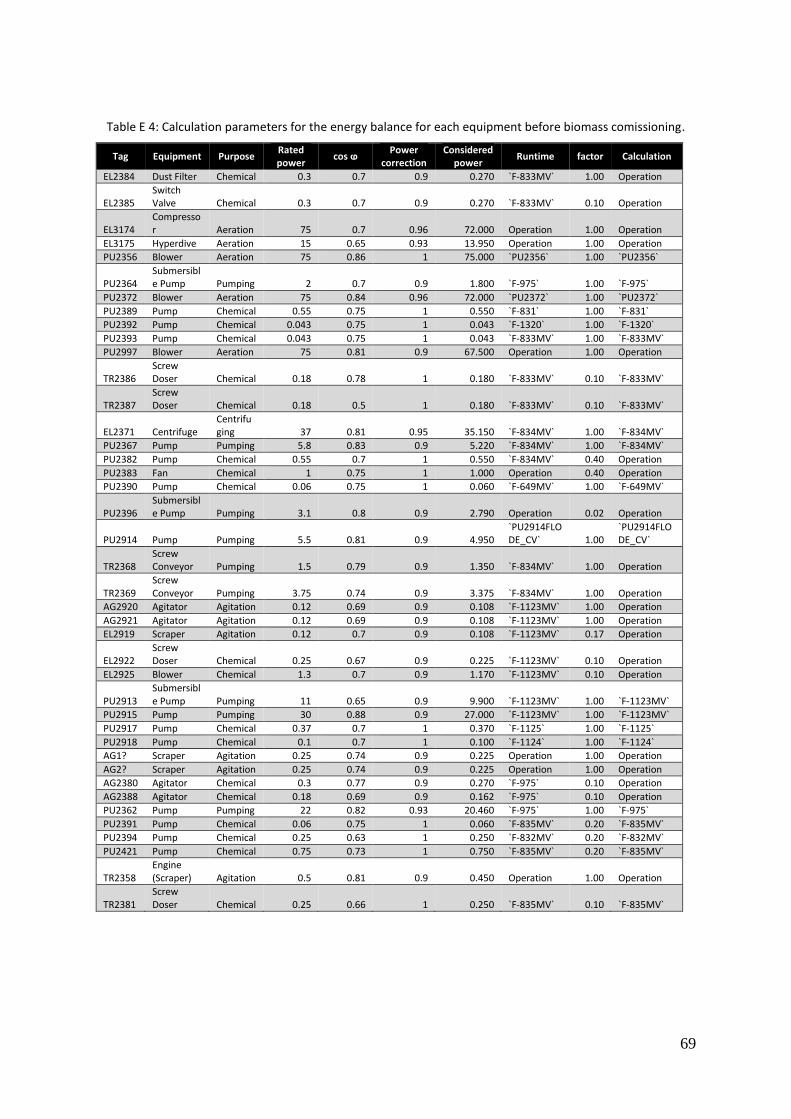
69
Table E 4: Calculation parameters for the energy balance for each equipment before biomass comissioning.
Tag Equipment Purpose Rated power
cos ⱷ Power
correction Considered
power Runtime factor Calculation
EL2384 Dust Filter Chemical 0.3 0.7 0.9 0.270 `F-833MV` 1.00 Operation
EL2385 Switch Valve Chemical 0.3 0.7 0.9 0.270 `F-833MV` 0.10 Operation
EL3174 Compressor Aeration 75 0.7 0.96 72.000 Operation 1.00 Operation
EL3175 Hyperdive Aeration 15 0.65 0.93 13.950 Operation 1.00 Operation
PU2356 Blower Aeration 75 0.86 1 75.000 `PU2356` 1.00 `PU2356`
PU2364 Submersible Pump Pumping 2 0.7 0.9 1.800 `F-975` 1.00 `F-975`
PU2372 Blower Aeration 75 0.84 0.96 72.000 `PU2372` 1.00 `PU2372`
PU2389 Pump Chemical 0.55 0.75 1 0.550 `F-831` 1.00 `F-831`
PU2392 Pump Chemical 0.043 0.75 1 0.043 `F-1320` 1.00 `F-1320`
PU2393 Pump Chemical 0.043 0.75 1 0.043 `F-833MV` 1.00 `F-833MV`
PU2997 Blower Aeration 75 0.81 0.9 67.500 Operation 1.00 Operation
TR2386 Screw Doser Chemical 0.18 0.78 1 0.180 `F-833MV` 0.10 `F-833MV`
TR2387 Screw Doser Chemical 0.18 0.5 1 0.180 `F-833MV` 0.10 `F-833MV`
EL2371 Centrifuge Centrifuging 37 0.81 0.95 35.150 `F-834MV` 1.00 `F-834MV`
PU2367 Pump Pumping 5.8 0.83 0.9 5.220 `F-834MV` 1.00 `F-834MV`
PU2382 Pump Chemical 0.55 0.7 1 0.550 `F-834MV` 0.40 Operation
PU2383 Fan Chemical 1 0.75 1 1.000 Operation 0.40 Operation
PU2390 Pump Chemical 0.06 0.75 1 0.060 `F-649MV` 1.00 `F-649MV`
PU2396 Submersible Pump Pumping 3.1 0.8 0.9 2.790 Operation 0.02 Operation
PU2914 Pump Pumping 5.5 0.81 0.9 4.950 `PU2914FLODE_CV` 1.00
`PU2914FLODE_CV`
TR2368 Screw Conveyor Pumping 1.5 0.79 0.9 1.350 `F-834MV` 1.00 Operation
TR2369 Screw Conveyor Pumping 3.75 0.74 0.9 3.375 `F-834MV` 1.00 Operation
AG2920 Agitator Agitation 0.12 0.69 0.9 0.108 `F-1123MV` 1.00 Operation
AG2921 Agitator Agitation 0.12 0.69 0.9 0.108 `F-1123MV` 1.00 Operation
EL2919 Scraper Agitation 0.12 0.7 0.9 0.108 `F-1123MV` 0.17 Operation
EL2922 Screw Doser Chemical 0.25 0.67 0.9 0.225 `F-1123MV` 0.10 Operation
EL2925 Blower Chemical 1.3 0.7 0.9 1.170 `F-1123MV` 0.10 Operation
PU2913 Submersible Pump Pumping 11 0.65 0.9 9.900 `F-1123MV` 1.00 `F-1123MV`
PU2915 Pump Pumping 30 0.88 0.9 27.000 `F-1123MV` 1.00 `F-1123MV`
PU2917 Pump Chemical 0.37 0.7 1 0.370 `F-1125` 1.00 `F-1125`
PU2918 Pump Chemical 0.1 0.7 1 0.100 `F-1124` 1.00 `F-1124`
AG1? Scraper Agitation 0.25 0.74 0.9 0.225 Operation 1.00 Operation
AG2? Scraper Agitation 0.25 0.74 0.9 0.225 Operation 1.00 Operation
AG2380 Agitator Chemical 0.3 0.77 0.9 0.270 `F-975` 0.10 Operation
AG2388 Agitator Chemical 0.18 0.69 0.9 0.162 `F-975` 0.10 Operation
PU2362 Pump Pumping 22 0.82 0.93 20.460 `F-975` 1.00 `F-975`
PU2391 Pump Chemical 0.06 0.75 1 0.060 `F-835MV` 0.20 `F-835MV`
PU2394 Pump Chemical 0.25 0.63 1 0.250 `F-832MV` 0.20 `F-832MV`
PU2421 Pump Chemical 0.75 0.73 1 0.750 `F-835MV` 0.20 `F-835MV`
TR2358 Engine (Scraper) Agitation 0.5 0.81 0.9 0.450 Operation 1.00 Operation
TR2381 Screw Doser Chemical 0.25 0.66 1 0.250 `F-835MV` 0.10 `F-835MV`
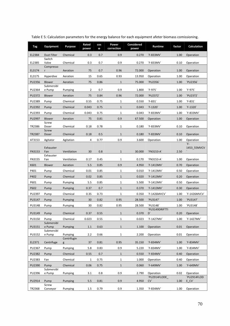
70
Table E 5: Calculation parameters for the energy balance for each equipment afeter biomass comissioning.
Tag Equipment Purpose Rated power
cos ⱷ
Power correction
Considered power
Runtime factor Calculation
EL2384 Dust Filter Chemical 0.3 0.7 0.9 0.270 `F-833MV` 1.00 Operation
EL2385 Switch Valve Chemical 0.3 0.7 0.9 0.270 `F-833MV` 0.10 Operation
EL3174 Compressor Aeration 75 0.7 0.96 72.000 Operation 1.00 Operation
EL3175 Hyperdive Aeration 15 0.65 0.93 13.950 Operation 1.00 Operation
PU2356 Blower Aeration 75 0.86 1 75.000 `PU2356` 1.00 `PU2356`
PU2364 Submersible Pump Pumping 2 0.7 0.9 1.800 `F-975` 1.00 `F-975`
PU2372 Blower Aeration 75 0.84 0.96 72.000 `PU2372` 1.00 `PU2372`
PU2389 Pump Chemical 0.55 0.75 1 0.550 `F-831` 1.00 `F-831`
PU2392 Pump Chemical 0.043 0.75 1 0.043 `F-1320` 1.00 `F-1320`
PU2393 Pump Chemical 0.043 0.75 1 0.043 `F-833MV` 1.00 `F-833MV`
PU2997 Blower Aeration 75 0.81 0.9 67.500 Operation 1.00 Operation
TR2386 Screw Doser Chemical 0.18 0.78 1 0.180 `F-833MV` 0.10 Operation
TR2387 Screw Doser Chemical 0.18 0.5 1 0.180 `F-833MV` 0.10 Operation
AT3153 Agitator Agitation 4 0.77 0.9 3.600 Operation 1.00 Operation
FN3153 Exhauster Fan Ventilation 30 0.8 1 30.000 `FN3153-A` 2.50
`F-1453_55MVCV`
FN3155 Exhauster Fan Ventilation 0.17 0.45 1 0.170 `FN3153-A` 1.00 Operation
K601 Blower Aeration 5.5 0.85 0.9 4.950 `F-1413MV` 0.70 Operation
P401 Pump Chemical 0.01 0.85 1 0.010 `F-1413MV` 0.50 Operation
P402 Pump Chemical 0.02 0.85 1 0.020 `F-1413MV` 0.20 Operation
P601 Pump Pumping 5.5 0.85 1 5.500 `F-1413MV` 0.50 Operation
P602 Pump Pumping 0.37 0.7 1 0.370 `F-1413MV` 0.30 Operation
PU2397 Pump Chemical 0.35 0.73 1 0.350 `F-1426MVCV` 1.00 `F-1426MVCV`
PU3147 Pump Pumping 30 0.82 0.95 28.500 `PU3147` 1.00 `PU3147`
PU3148 Pump Pumping 30 0.82 0.95 28.500 `PU3148` 1.00 `PU3148`
PU3149 Pump Chemical 0.37 0.55 1 0.370 `PU3149DRIFTTID` 0.20 Operation
PU3150 Pump Chemical 0.023 0.55 1 0.023 `F-1427MV` 1.00 `F-1427MV`
PU3151 Submersible Pump Pumping 1.1 0.63 1 1.100 Operation 0.01 Operation
PU3152 Submersible Pump Pumping 2.2 0.66 1 2.200 Operation 0.01 Operation
EL2371 Centrifuge Centrifuging 37 0.81 0.95 35.150 `F-834MV` 1.00 `F-834MV`
PU2367 Pump Pumping 5.8 0.83 0.9 5.220 `F-834MV` 1.00 `F-834MV`
PU2382 Pump Chemical 0.55 0.7 1 0.550 `F-834MV` 0.40 Operation
PU2383 Fan Chemical 1 0.75 1 1.000 Operation 0.40 Operation
PU2390 Pump Chemical 0.06 0.75 1 0.060 `F-649MV` 1.00 `F-649MV`
PU2396 Submersible Pump Pumping 3.1 0.8 0.9 2.790 Operation 0.02 Operation
PU2914 Pump Pumping 5.5 0.81 0.9 4.950 `PU2914FLODE_CV` 1.00
`PU2914FLODE_CV`
TR2368 Screw Conveyor Pumping 1.5 0.79 0.9 1.350 `F-834MV` 1.00 Operation

71
TR2369 Screw Conveyor Pumping 3.75 0.74 0.9 3.375 `F-834MV` 1.00 Operation
AG2920 Agitator Agitation 0.12 0.69 0.9 0.108 `F-1123MV` 1.00 Operation
AG2921 Agitator Agitation 0.12 0.69 0.9 0.108 `F-1123MV` 1.00 Operation
EL2919 Scraper Agitation 0.12 0.7 0.9 0.108 `F-1123MV` 0.17 Operation
EL2922 Screw Doser Chemical 0.25 0.67 0.9 0.225 `F-1123MV` 0.10 Operation
EL2925 Blower Chemical 1.3 0.7 0.9 1.170 `F-1123MV` 0.10 Operation
PU2913 Submersible Pump Pumping 11 0.65 0.9 9.900 `F-1123MV` 1.00 `F-1123MV`
PU2915 Pump Pumping 30 0.88 0.9 27.000 `F-1123MV` 1.00 `F-1123MV`
PU2917 Pump Chemical 0.37 0.7 1 0.370 `F-1125` 1.00 `F-1125`
PU2918 Pump Chemical 0.1 0.7 1 0.100 `F-1124` 1.00 `F-1124`
AG1? Scraper Agitation 0.25 0.74 0.9 0.225 Operation 1.00 Operation
AG2? Scraper Agitation 0.25 0.74 0.9 0.225 Operation 1.00 Operation
AG2380 Agitator Chemical 0.3 0.77 0.9 0.270 `F-975` 0.10 Operation
AG2388 Agitator Chemical 0.18 0.69 0.9 0.162 `F-975` 0.10 Operation
PU2362 Pump Pumping 22 0.82 0.93 20.460 `F-975` 1.00 `F-975`
PU2391 Pump Chemical 0.06 0.75 1 0.060 `F-835MV` 0.20 `F-835MV`
PU2394 Pump Chemical 0.25 0.63 1 0.250 `F-832MV` 0.20 `F-832MV`
PU2421 Pump Chemical 0.75 0.73 1 0.750 `F-835MV` 0.20 `F-835MV`
TR2358 Engine (Scraper) Agitation 0.5 0.81 0.9 0.450 Operation 1.00 Operation
TR2381 Screw Doser Chemical 0.25 0.66 1 0.250 `F-835MV` 0.10 `F-835MV`