Keskustelualoitteita #48 Joensuun yliopisto, Taloustieteet

Criminal career and age-crime profile

Mikael Linden

ISBN 978-952-458-979-6 ISSN 1795-7885

no 48

CRIMINAL CAREER AND AGE-CRIME PROFILE

Mikael Linden Economics and Business Administration University of Joensuu, Finland (mika.linden@joensuu.fi)

JUNE 2007

Abstract

Two classical issues in criminology, criminal career paradigm and age-crime curve rule, are analyzed in terms of economics. Age-crime curve sums up the crime intensity and participation aspects of individual crime behaviour during his/her lifetime. It is argued that crime intensity must be the starting point of economic analysis if we want to understand crime career and age-crime curve regularities. A simple model with crime intensity as age dependent decision variable was proposed to generate non-homogenous life time crime intensity rate. The bell shaped age-crime alternative was tested empirically with arrest count data of felony defendants in large urban counties in U.S year 1998. Poisson and NegBin count data regression models gave unsatisfactory results concerning the age dependency of number of arrest counts. NLS regression on individual age standardized arrest counts and semi-parametric Poisson regression on individual arrest counts provided acceptable results. The semi-parametric model estimation allowed for non-homogenous crime intensity presentation in the form of age class average proportional intensities. Regardless of using age standardized counts or controlling for avarage age-dependent intensities the bell shaped age-crime profile was not rejected for the sample.

Key words. Criminal career, age-crime profile, non-homogenous Poisson process, count data regression models, semi-parametric estimation.

I. Background There are two topics that have excited much debate in recent criminology literature. The

older one, criminal career paradigm, refers to basic empirical requirement for

characterizing criminality as a career, the autocorrelation of criminal behavior. The

probability to commit a crime is higher for individuals that have already a criminal record

compared to individuals without one. The second topic is the most important empirical

regularity in criminology, the age-crime curve: however or wherever measured the rates

of criminal involvement in the population is highest for the young (males) between ages

17 to 25 (Land & Nagin 1993). Although these facts are not in accordance with each

other in all cases (e.g. life-course criminals) they are typically closely inter-connected.

Age-crime curve predicts that a gradual decline will take place in average crime rates

among the older age cohorts. This fact does not rule out the state dependency predicted

by criminal career paradigm. State dependency can still occur among the careerists

although increasing number of criminals terminates their criminal career and crime

intensity is small in the old age cohorts.

Basically criminal age or time dependency (age-crime curve) and state dependency

(criminal career and recidivism) are conceptually distinct - the former refers to particu-

lar age (or time) structure among the criminals, and the latter refers to non-time

dependent clustering (stigmatization, lock-in or hysteresis phenomena) of criminal

actions among some criminals. Nevertheless they are empirically closely related since

criminal activity is determined by the criminals’ discounted lifetime, and once started

criminality at youth breeds too often new crimes. Thus overall volume of crime is

therefore a function of frequency and prevalence (participation). The crime frequency

does not decrease as much with age as participation (Kyvsgaard 2003, Ch. 7-8). This

particular two dimensionality of criminality is also harmed by many measurement biases

(e.g. what is the proper and reliable unit of measurement of criminality, sample selection

in analyzed data, individual unobserved heterogeneity, etc.) and conceptual problems

(e.g. how to define the criminal career, changing legal norms and sanctions, etc.). In spite

of these problems criminal career paradigm and age-crime curve are still major research

1

agendas in criminology (e.g. Fagan & Western 2005, D’Unger, Land & McCall 2002,

Levitt 1999).

However a more deeply problem lies in the disagreement concerning the theoretical

understanding of age-crime curve and criminal career. Criminal (choice) career theory

(Blumstein & Cohen 1979) underrates the age-crime curve much as statistical artifact but

the criminal propensity theory (Gottfredson & Hirschi, 1990, 1983) stresses the lack of

self-control and unsocial behavior of teenagers. Recently evolutionary psychology has

give support the propensity theory with argument that age-crime curve is produced by the

difference between the reproductive benefits and costs of competition among young men

(see Campbell, 1995, Kanazawa 2002). The well developed modern statistical theory

provides models that can test the implications of both theories (e.g. Land 1992, Nagin &

Land 1993, Blumstein 2005). The results support both theories. The outcome is expected

remembering the dimensions of criminality. Aggregate age-crime curve is a product of

both the high rate of youth full participation in crime, and the high activity level (crime

frequency or intensity) of these young offenders. Age specific differences in

participation, however, rather that frequency, are primarily responsible for the basic form

of the age-crime curve (Kyvsgaard, 2003, p. 106).

Economic theory does not have much to say about age-crime curve phenomena but

criminal career issue can be understood by it in some extension. Heineke (1978)

categorizes economic models of crime as either (1) portfolio problems, in which the agent

must decide how much wealth to put risk through involvement in crime, or (2) labour

supply problems, in which the agent must choose the amount of time to be allocated to

illegal activity. In both cases criminal activity onsets if the expected net gain or utility

from it exceeds the benefits from legal activity. In principle a repeated activity

(recidivism) can be modeled as a sequence of crimes where prolonged activity can be

seen as means to accumulate (illegal) capital or consumption resources. As the activity

can be halted by imprisonment the incentive to return to illegal activity after sentence is

high as typically the capital gained from crimes is confiscated by state. This kind of

career optimization can been modeled with dynamic programming methods including

2

three conditional states (terminated activity, halted activity, repeated activity) where the

life time expected net income is maximized. Leung (1991, 1995) provides a nice starting

point to these models. His approach resembles closely to technically demanding job

change and career literature found in modern labour economics (e.g. Berkovic & Stern

1991, Hopenhayen & Rogerson 1993, Rust 1996, Adda & Cooper 2003). However many

questions are still open and much work is needed to get transparent and robust economic

models of recidivism.

The main problem with the approach above is that it can reveal only some issues on

property crimes – not crimes in general. Secondly, it is silent of age-crime curve or

profile regularity. By adding some elements of human capital and portfolio theory to the

career optimization model would support age-crime curve, since relative expected gains

from crimes of young person are high as their wealth is very low and first round

sentences are not severe. Leung’s paper (1994) on economics of age-crime profile is a

promising starting point in this context. He observes first that two dimensionality of

unimodal and positively skewed age-crime profile relates to the above underlying

concepts of ‘age-participation’ and ‘age-intensity’. The former can easily explain the age-

crime profile but surprisingly Leung argues that changes in the latter can alone explain

the age-crime profile.

The key of this result lies in the selection effect, i.e. intensity rate of offending increases

with age and the hazard rate of arrest rises over time. An increasing hazard rate of arrest

implies that fewer offenders can successfully avoid arrest as they got old. As a result, the

proportion of older offenders is smaller because many of them had already been

apprehended when they were young. The observed age-crime profile indicates a more

intense selection among the young offenders because it is more difficult to sustain

criminal career involving more serious offenses for an extended period of time (Leung

1994, p. 483-84). Leung’s basic economic argument for increasing crime intensity rate

stems from the consumption-investment decision theory. The probability that criminal

will not be arrested by time t is like a capital asset that has to be consumed in the finite

lifetime. A dynamic trade-off exists between consumption and capital de-accumulation.

3

An optimal strategy is to increase the intensity (i.e. consumption) over life time as the

expected returns form criminal activity fall over the finite life time. If criminal would

exhaust the stock of capital too early, he/she would not be able enjoy any later gains at

all, resulting in a lower lifetime expected utility. The increase in the intensity rate over

time is driven by the end-of-horizon effects.

Although Leung’s approach is challenging and novel it has some drawbacks. First, the

analogy to capital theory is somewhat awkward. If the criminal’s subjective interest rate

(time preference) is high and he/she is risk-aversive the increasing intensity rate is not

necessarily sustained. Second, to derive the observed age-crime profile it is enough that

the age-intensity profile has the same form, i.e. the intensity rate of offending increases

rapidly in the teens and then start to decline after 25 years. However we do not have yet

an economic theory to support this behaviour. Leung’s trick to derive observed age-crime

profile with increasing intensity rate is the selection effect. It is difficult to maintain a

criminal career with an increasing intensity rate of offending over an extended period of

time. Thus there exist less offenders in old age cohorts compared to young ones. Third,

Leung does not deal with the issues of criminal career and recidivism. He only derives

optimal time for first crime action with increasing intensity rate. Thus Leung’s approach

can give one answer to observed age-crime statistics but many other underlying aspects

remain unexplained. However other economic papers that pay theoretical attention to

dynamic complexity of criminal activity are few (Davis 1988, Polinsky & Rubinfield

1991, Lee & McCrary 2005, Jacob, Lefgren & Moretti 2004) 1).

In this context a simple model that tackles the salient features of crime career and age-

crime curve is proposed. The starting point of the model is the fact that crime intensity

per time and age varies across the individuals and they control their intensity. Higher

activity increases the probability of imprisonment. The criminal sets his crime rate at

level that minimizes his expected time devoted to criminal activity incurring some costs.

_____________________________________________

1) Two last mentioned references give also partial review of current related literature. The special number of Int. Economic Review (Vol. 45, Number 3, 2004) on Economic Models of Crime contains also some important papers.

4

By augmenting the basic model with fixed expected life time during the total number of

crimes can be committed we are able to show that increased number of crimes increases

the expected life time with rate that increases also the life time crime intensity. This

result gives an explanation to question why old criminals necessarily do not commit less

age standardized crime than young ones (the intensity effect). The assumption of age

dependent subjective time preference stresses the model results that crimes are committed

at the beginning of life time. The model emphasizes the noticed importance of finding a

connection between behavioral models and stochastic models of crime.

In the empirical part of paper some statistical models related to Poisson regression are

suggested and estimated. However used crime career data (BJS, 1998) and implications

of economic model refer to non-homogenous Poisson process for crime intensity. Thus

some modifications of the basic Poisson regression – both parametric and semi-

parametric - are proposed. Results show that age-crime curve is still valid although we

control for observed personal characteristics and for average age cohorts effects of

individual recidivism.

II. Model of crime intensity, criminal career, and age-crime profile II.1. Optimizing the crime career

Assume that measurable criminal activity rate (intensity) (i.e. number of crimes during

given time interval, e.g. ) takes values between 0

v

/s year and MAXv , i.e.

(I.1) , when 0 , and

.0, when and 0

MAX

MAX

v v vv

v v v≤ ≤⎧

= ⎨ > <⎩

It is assumed that activity is distributed uniformly between 0 MAXv v≤ ≤ . Naturally none

activity takes place when and at rate 0v ≤ MAXv v> when a sure arrest happens. Higher

the activity, the higher is the probability that it is stopped by the control authorities.

Structure of Eq. 1) gives a linear relationship between activity and the probability of

being stopped

5

(I.2) [ ] ( ) 0 , where 1/ .MAX MAXProb V v p v kv v v k v≤ = = ≤ ≤ =

The person is detained for average time . The random number of authorities in

proximity to criminal activity has a Poisson distribution with a parameter

0t

μ . Assume that

number of crimes person commits is . Now the average or expected time S [ ]E t of

committing these crimes or criminal career, which includes also the imprisonment time,

is

(I.3) 0 0[ ] / ( ) / .E t S v Sp v t S v Skvtμ μ= + = +

The rational criminal tries to minimize the expected time devoted to number of crimes

with optimal criminal activity rate value

S

* (0, )MAXv v∈ . Thus we have assumed that

criminal has chosen a criminal career and he/she is maximizing the net benefits from it.

Since high value of gives a possibility to commit many crimes and at same time it

increases the probability of arrest the rational criminal looks for a minimizing value of

that gives an optimal trade off value between these opposite factors. Optimizing Eq.

3) in respect to

v

*v

v

(I.4) 02

[ ] 0dE t S Sktdv v

μ= − + =2

2 3

[ ] 2 | ( 0 )d E t Sdv v

= >

gives a solution that is independent of *v S

(I.5) 0 0

1* MAXvvkt tμ μ

= = (0

1* if MAX MAXv v vtμ

< > ).

The first order condition for optimal crime activity

(I.6) 02

1 0ktv

μ− + =

entails following comparative statistic results

6

(I.7) * * *0

0, 0, and 0. v v v v v vdv dv dvd dk dtμ = = =< < <

Thus an increase in control activity μ , a decrease of maximal crime rate, and an increase

of arrest time decreases the optimal crime number per time unit. Subsequently the

expected time t of crime career increases for fixed crime intensity and S when the

control parameters increase (see Eq. I.3). Thus we run into same number of crimes as

earlier but now they are committed during the longer time period. Contrary to this

typically the parameters

*v

0, , and k tμ are lower for first time and young criminals

supporting high crime intensity rates for them.

The model above is in many ways too general or abstract to analyze all salient questions

concerning the crime activity and life time crime career. However it gives some support

for inverted U-shaped crime-age profile. Note also that optimal result for crime intensity

was surprisingly independent of participation activity but the optimal v S | *[ ] v vE t =

depends positively on S. In following three modifications are introduced into the model.

First we notice that v is the crime activity during the whole expected life of criminal

[ ]E T and v s . Now as (fixed) expected life time '/ [ ]E T= [ ]E T is the maximal total

expected life time devoted to criminal activity [ ]E t and the criminal optimize with we

must have . Second we assume that the probability of arrest is a convex function

of crime activity during the expected life time. Thus

v

's S=

(I.8) [ ] ( ) 0 , where 1/ with 1.aMAX MAXProb V v p v kv v v k v α≤ = = ≤ ≤ = >

Note that with 0 1α< < , high criminal activity entails that the probability of arrest

increases slowly. However when 1α > the arrest probability is low for low levels of

activity but the arrest probability increases rapidly with activity level. We consider only

the latter case. Finally we assume that criminal activity incurs additional costs with a

convex cost function depending on the number of crimes, i.e. . The mini-

mization problem of the average length or expected criminal career

2( / 2)Sβ

[ ] [ ]E E Tτ ≤ is

7

(I.9)

20

12

0

[ ] [ ]2

[ ] .[ ] 2

E E T Skv t S

SE T kt SE T

α

α

α

βτ μ

βμ+

= + −

= + −

As the number of life time crimes is now the only variable of model the criminal

minimizes with it the expected life time devoted to criminal career. The first order

condition is

S

(I.10)

0

1 * 1

0

[ ] ( 1) [ ] 0

[ ] ( ) 0 : , where 0.( 1)

dE kE T t S SdS

E Tg S S B S B Bkt

α α

αα α

τ α μ β

βα μ

−

− −

= + − =

⇒ = − = = = >+

A minimum exists since*S2

*2

[ ] |S Sd E

dSτ

= > 0 (see Appendix I). Note that for any

parameter values of (see Appendix II) 1a >

(I.11) *[ ] 0S S

dE TdS = > , *

[ ] 0S SdE T

dμ = > , *[ ] 0S S

dE Tdk = > , *

0

[ ] 0S SdE T

dt = > .

These results mean that if the criminal keeps his criminal participation at the optimal

level that sustains the optimal minimized expected time devoted to this activity, then

an increasing number of crimes must be compensated with higher expected total life time.

In similar fashion if the control activities increase (

*S

00, 0, 0)d dk dtμ > > > the expected

life time increases. The result is called the paradox of crime career. In the fight against

criminality the society increases the expected life time of careerist and his/her number of

crimes. The paradox lies in the existence of optimal value of number of crimes per life

8

time once the career of criminality is chosen: higher the expected life time among the

criminals, larger is the number crimes devoted to minimize the length of expected

criminal career.

II.2. Age dependent crime intensity and time preference

The results obtained above support the bell-shaped age-crime curve regulatory since we

can argue that young criminals have higher crime intensity than older criminals, and

longer is expected life time of criminal larger is the number of crimes committed by the

person. Thus we have a prediction that crime participation is distributed evenly during the

life time but the intensity varies. Note however that 0/dS dt 0< at participation optimum.

The crime participation decreases when the average imprisonment time increases. This is

the selection effect that reduces the number of older criminals among the population.

The selection story is however deeper one in this context since

with optimum (see App. II). The result indicates that optimum participation level can

be only sustained with expected life time with rate that is larger than life time intensity

rate. Note however that if

/ [ ] / [dS dE T v S E T> = ]

*S

[ ]E T refers to the expected remaining life time among the

careerist then we observe two things.

First, as the expected life time decreases with age the number of crimes decreases also

but with a higher degree, i.e. life time crime intensity / [ ]v S E T= can still be high

although the level of participation S and (remaining) expected lifetime [ ]E T are low. A

lower participation among older criminals is obtained if look in details the expected life

formula, i.e.

(I.12) 0 0 0

[ ] ( ) ( ) [1 ( )]E T tf t dt G t dt F t dt∞ ∞ ∞

= = = −∫ ∫ ∫

where is the probability to live at least t years, and

is survival probability of living past years. A most

elementary model of life time distribution that also has some relevance in human

( ) [ ]F t Prob T t= ≤

( ) 1 ( ) [ ]G t F t Prob T t= − = > t

9

populations is the exponential distribution. As ( ) tG t e φ−= ( 0, 0t )φ≥ > for exponential

distribution, we have

(I.13) 0

1 1[ | ] [1 ]t x

tE T t e dxe

φφφ

−< ∞ = = −∫ .

Now

(I.14) *[ | ]

S SdE T t

dS =

< ∞=

1 1[ [1 ]]0

tde

dS

φφ−

>

can happen only with increasing age if since 0dt > 0dS >

(I.15) 1 1[ ] ttd e d

eφ

φφ φ−− = > 0t .

Thus the number of crimes decreases with less additional years of life. Note that other life

time distributions can give opposite results and challenging our basic result that

*[ ] 0.S S

dE TdS = >

Secondly, the form of time preference for the remaining life may alter the result too. In

Appendix III it is shown that an age exists where turns negative when expected

life time is valued with decreasing time preference when age increases , i.e.

/dS dt

( 0dt > )

t( *) with '( *) 0,r te r t− < where * *t T= − . Thus if the criminal values his remaining

planned life time highly, then the number of crimes decreases, i.e. 0dSdt

< when ,

and

1t t>

*[ ] 0S S

dE TdS = < .

10

III. Statistical models of arrest counts Assume at the arrest time the criminal i has experienced during his lifetime

number of earlier arrests denoted as

0t iT

0|i t ty < . Naturally 0|i t t iy < y= can take only finite

number of non-negative integer value like 0,1,2,....iy = Assume that iy measures the

criminal career of person i before time . This type of phenomena is called a count

process { , , where is the number of events that have occurred before time

The process is called a Poisson process if the probability of a single occurrence during a

brief time interval (exposure time t ) is proportional to its duration and if the occurrences

in two non-overlapping intervals are independent. Now the probability function of Y has

the form

0t

}tY t +∈ tY 0 .t

(II.1) ( )( ; , ) ( ; , ).!

t y

i ii

e tf y t Poisson y ty

λ λλ λ−

= ∼

The Poisson process can be characterized by exponentially distributed waiting times

between consecutive events leading to a time-invariant hazard function. This observation

(with ) leads to Poisson –regression model that is a natural starting point in many

applications. Thus

1t =

iy , given the vector of regressors , is independently Poisson

distributed with density

ix

(II.2) ( | ) , 0,1, 2,...!

i iyi

i ii

ef y y

y

λ λ−

= =ix .

The mean parameter is

(II.3) exp[ ],iλ = ix 'β 1, 2,....,i N=

where β is ( 1)xk parameter vector.

11

However this set-up is not applicable for crime career data analyzed in this paper. The

reason is two fold. First we have data for different person with different arrest numbers

iy during his/her life time (i.e. his/her age) up till time point . Naturally in average

older criminals have larger crime record than young criminals. Second we have argued

that crime intensity is not constant but it is age dependent (i.e. the age-crime curve). This

means that basically in Eq. 1)

iT 0t

iλ is time dependent, i.e. ( ) for 0i t tλ > and the Poisson

process is now non-homogenous. Thus we allow for possibility that arrests may occur

more likely during certain periods of life time than during other times, i.e. the age-crime

profile. We also note that exposure time . i it T≠ Typically it Ti< since we can not assume

that all criminals devote their entire life time to criminal career.

Figure 1. depicts the situation graphically. Person A is relative young (say above 15

years) but has already experienced two arrests. Person B with age of 28 has already a

large and increasing crime record. Person C is in his middle ages but his criminal career

has started quite late. Person D has a criminal career motivated by our theoretical model.

Most of arrests happens at younger years and they decay at later years.

Figure 1. Crime careers and ages

12

Note that in the Poisson regression model

(II.4) [ | ] [ | ] exp[ ].i i i iE y VAR y= = ix x x 'β

Thus the conditional mean and variance are equal. The model assume that relevant

individual factors that cause arrest counts are contained in vector . These are typically

variables like sex, race, occupation and age. The last one is relevant in our case. Our

hypothesis is that age dependency of criminal career is non-linear: first increasing in

younger years and then decreasing at older ages. This can be modeled with 2

ix

nd order age

polynomial like 20 1 2( )f T a a T a T= + + . The functional form corresponds to our predicted

criminal age profile with . Thus the base model have form of 1 0 and a 0a > 2 <

[ | ]i iE y =x , ,1exp[ ] exp[ ( )]k

j i j i ijb x f T

== +∑ix 'β .

Note that model is based on the homogenous Poisson process, i.e. λ is constant. Our

theoretical model, like Leung’s model, leads to an interesting notion that a criminal can

“speed up” his crime activity given the time of his/her life devoted to criminal active

conditioned on the arrest probability. This observation entails a case where the length of

count exposure time varies across the individuals, i.e. the expected count is proportional

to the length of the interval during it has occurred. Now for the individual time of

exposure homogeneous Poisson process entails that it

(II.5) exp[ ( )] exp[ ( ) ln ]i i i i it f T f T t= + = + +i ix ' x 'β β 1, 2,...,i N=, . λ

13

A) OLS and NLS estimation

Eq. II.5) gives an interesting possibility for OLS estimation since under assumption that

we can use approximate model it T= i

) i

(II.6) ˆ / (i i i iT g Tλ λ ε= = + +ix 'β .

Thus we have a regression model that is not anymore based on counts and Poisson

distribution but on exposure time age standardized “counts” with [ ] 0iE ε = . Estimation

of Eq. 6) gives us some preliminary information concerning how individual factors affect

arrest intensity per age. Note also that standardization leads also to age function

where our crime career age profile hypothesis corresponds to

An alternative estimation is based on NLS-method. The method

produces less biased results compared to OLS under assumption that Poisson approach is

true one.

0 1( )g T a a T= +

0 10 and 0.a a> <

i

(II.6’) ˆ / exp[ ( )]i i i iT f Tλ λ ε= = +ix 'β + .

Note with assumption 2(0, )i NID εε σ∼ NLS equals MLE, and it gives consistent

estimator for model parameters. However the efficiency loss is evident since NLS ignores

the inherent heteroskedasticity of Poisson regression.

B) Poisson Regression and unobserved heterogeneity

Holding back to integer count numbers and Poisson model

(II. 7) exp[ ( )] exp[ ( ) ln ]i i i i it f T f T t= + = + +i ix ' x 'β β 1, 2,...,i N, = , λ

14

we observe that this formula is problematic since it contains both exogenous time effect,

= age, and endogenous time effects, the optimal criminal career (= exposure time).

Typically, like in this study, we do not have data for criminal’s exposure time (or the

period of risk) for criminal activity, i.e. waiting times between subsequent arrests or his

total crime career period. One crude solution (used already above in Eq. II.6) is to assume

that meaning that criminal’s age equals the crime exposure time. Note that this

result was obtained in our theory model above. Obviously they differ but they are

expected to be highly correlated at least for life career criminals. This notion makes the

statistical estimation of Eq. II.7) unreliable. However we can assume that and are

related to each other randomly, i.e.

iT it

it T= i

i

iT it

i it Tε= where iε is some random variable defined on

limits . Thus part of person’s life is selected randomly to the criminal career. This

formulation preserves some age dependence on exposure time. Alternatively we can

argue that we can not measure correctly. We only observe that is augmented with

measurement error

(0,1)

it iT

iε to correspond the unobservable . it

The main weakness of Poisson model is the assumption that

stemming from the fact that the intensity of Poisson process is a deterministic function of

the covariates. No unobserved heterogeneity is allowed for. Likewise assumption of

independent random counts over time is questionable, i.e. occurrences influence the

probability of future occurrences (positive count occurrence dependency or positive

contagion). Unobserved heterogeneity and positive contagion lead to over-dispersion

phenomena . The former is easily seen if we assume that

[ | ] [ | ]i i i iE y VAR y=x x

[ | ] [ | ]i i i iE y VAR y<x x

i

(II.8) exp[ ] exp[ ]i iλ ε μ= + =i ix ' x 'β β

where captures the non-modeled unobserved heterogeneity and iu [ , ] 0i icorr ε =x . Now

[ ]iE iλ λ= and of 2 2[ ]ii iVAR uλ λ σ= if we scale [ ] 1iE μ = . Thus

15

(II.9) 2 2

[ ] [ [ | ]] [ [ | ]]

[ ] [ ] .i

i i i i

i i i i u

VAR y E VAR y VAR E Y

E VAR

λ λi

iλ λ λ λ σ λ

= +

= + = + >

Note that above we proposed the alternative that i it T iε= . Now noticing this in Eq. II.8)

gives

(II.10) exp[ ln( ) ] exp[ ln ln ] exp[ ]i i i i i iT T T iλ ε ε= + = + + =i ix ' x ' x ' εiβ β β .

Eq. II.10) gives the possibility to use age as exposure time variable but the price is the

over-dispersed count model that is not anymore a Poisson process model. The

specification in Eq. 10) entails that we can use once again function 2

0 1 2( )f T a a T Tα= + + with to preserve the argued inverted U -shape

age response to arrests counts. Note that specifications in Eq. II.7) and Eq. II.10) imply

that we have to use parameter constraint

1 21 and 0a a> <

1θ = in the models

(II. 7’) exp[ ( ) ln ] exp[ ( )]i i i i if T t t f Tλ θ= + + = +i ix ' x 'β β ,

(II.10’) exp[ ( ) ln( ) ] exp[ ( )]i i i i if T T T f Ti iλ θ ε= + + = +i ix ' x 'β β ε .

These specifications support the basic assumption of count models that intensity rate iλ

is constant and preserve the proportionality to exposure time, i.e. doubling the exposure

time doubles the expected number of counts. Form point of view of age-crime curve

testing this means that rejecting the constraint 1θ = refers to non-homogenous Poisson-

or count process where the exposure time affects the number of counts in non-linear way.

This means that age and exposure time are partly endogenously selected to number of

crimes, not only exogenously determining them. Thus rejecting the hypothesis 1θ = for

alternative 1θ > in the presence of 20 1 2( )f T a a T a T= + + in the model is actually test

for age-crime curve hypothesis augmented with indication of deeper level age

16

dependency of crime rates. Note that it is quite easy to show that if ( | )i t ageλ is

increasing function of age we have the case of [ | ] [ | ]i i i iE y VAR y<x x

x

once again.

Thus the equality of conditional expectation and variance is not realistic assumption for

many applications of count data. The over-dispersion case is also evident under the

presence of positive occurrence dependence.2) Much used Negative Binomial (NegBin)

model alternative allows for over-dispersion, i.e

(II.11) 2 2[ | ] [ | ] [ [ | ]]i i i i i iVAR y E y E yσ= +x x

leading to model alternative also for the conditional variance

(II.12) 2 1 exp( ' )iσ = + iz γ ,

where iz is vector of some explanatory variables. When 1γ = we get a scalar dispersion

parameter, otherwise we estimate a variance function. Some more general models allow

for under-dispersion (see Winkelmann & Zimmermann 1995, Winkelmann 2003,

Cameron and Trivedi 1998). Negbin –model alterative can easily to show preserve

positive occurrence dependence. If an arrest occurrence increases the probability of next

occurrence then the Polya urn schema gives NegBin distribution.

___________________________________. 2) Negative contagion causes underdispersion. This can be seen in following way

0, for 0

Pr [ ]( , ) ( 1, ), for 1, 2, ...

.r

ob Y rPoisson r Poisson r rα α

== =

− + =

⎧⎨⎩

If 1α > (the parameter for positive duration dependence in Gamma distributed waiting time) then Poisson count process exhibits under-dispersion (Winkelmann 1995). Note that positive contagion (negative duration dependence) can also rise from aggregation of individuals having different waiting times (i.e. different propensity to experience an event).

17

We stress that above developments and comments do not imply that we have solved the

statistical problems of unobserved heterogeneity and (positive) contamination - far from

it. We have only shown that all assumptions of Poisson model are not fulfilled in our

model specification of arrest counts and suggested specification of age effects leads to

richer model alternative. One alternate to be estimated combines normal distributed

unobserved heterogeneity in NegBin –model.

C) Semiparametric estimation

The Poisson equi-dispersion model can still be questioned when we face non-

homogenous Poisson process ( )i tλ for observed counts. A partly solution to this problem

is to use richer functional presentation for exposure time effects in Poisson model, i.e. we

have to have model like

(II.13) ( ) ( ) exp[ ]i it g tλ = ix 'β ,

where is a some function that models the time (e.g. age) dependent crime event

occurrence rate. The model in Eq. II.13) allows us to separate the age class effects and

individual age effects on crime counts. measures the age class effects, and -

still including

( )ig t

( )ig t ix '

20 1 2( )f T a a T a T= + + - measures the individual crime rate effects.

Because our sample of age observations is used to model both these effects some special

model and estimation alternative are used.

Assume next that non-homogenous Poisson process with time dependent intensity

function fulfills the following proportional property

(II.14) 0( ) ( )exp[ ],i it tλ λ=x ix 'β

where 0 ( )i tλ is the baseline intensity function. The corresponding cumulative or

integrated intensity function is

18

(II.15) 00

( ) ( ) ( ) exp[ ' ]t

i i i it u du tλΛ = = Λ∫x x x β ,

where . Suppose that there are independent observations on

individuals and he/she is observed over the time interval . Let be events (arrests)

observed to occur at times . Given the age information we can always

order ’s so that with . Letting

0 0( ) ( )ti t uλΛ = ∫0 du

n

n

m

(0, )iT in

1 2 ....ii i it t t< < <

iT 1 20 .... mT T T< ≤ ≤ ≤il iT t≥ 0 0T = and represent

the total number of events (arrest) in (0 , we can write for

( )n t

, )t 1, 2,...,i m=

* *1 0 0 1[ ( ) ( )] [ ( ) ( )] exp( ' )m

i i l iE n t n T t T− − =

− = Λ − Λ k∑ x β , for , 1i iT t− < ≤ T

where corresponds to *0 ( )tΛ 0*

0 0( )t eβλ λ= . Note that in this application context both

refer to different age classes, i.e. we estimate average proportional age class

crime intensities.

and it T

This suggest the estimate for 1, 2,..., i m=

(II.16) 1

1* 10 ˆ ˆ' '

1

( ) ( ) ( ) ( )ˆ ( ) ,i i

l li

i

in n i

m mn

l n l i

n T n T n t n Tte e

−− −

== =

− −Λ = +∑

∑ ∑x xβ β 1i iT t− T< ≤ .

Eq. II.16) entails a two step estimation routine with equations

(II.17a) '*2

01 1ˆ ( ) 0, 1, 2,...,i

m mi ir i iri i

r

l n x T x e r kβ = =

∂= − Λ = =

∂ ∑ ∑ x β

and

(II.17b) 1

1*0 ˆ'

1

( ) ( )( ) , 1, 2,.., ,i i

li

i

in n

i mn

l n

n T n TT i

e

−−

==

m−

Λ = =∑∑ x β

19

where l2 is the loglikelihood from likelihood * *1 0 2 0( ) ( , )L LΛ Λ β . Thus we estimate first

from Eq. II.17b) with by setting *0 ( )iTΛ = 0β and then by using the gradient condition

II.17a) a ML –estimate is obtained for β̂ . Inserting this back in II.17b) provides a

new estimate for . By repeating this iterative 2-step produce convergent estimates

for

*0 ( )iTΛ

*0 ( ) and iTΛ β are obtained (for more details, see Lawless 1987). In principle this

method separates and estimates the average proportional age class intensities and

individual control effects on observed individual crime counts.

IV. Data and Estimation Results IV.1. Data Our data consists of felony defendants in large urban counties in U.S in year 1998

(USDoJ/BJS: State Court Processing Statistics, 1998). In the 1990’s Bureau of Justice

tracked every second year a sample of felony cases during the month of May in 75 largest

counties in the US. Thus the follow up (or sample exposure) time is one month. The

original sample consisted of 15878 arrested individuals with following variables

0t

PRIARR = Number of prior arrests (0,1,2,….,N), AGE = Age of defendant.

PRICONV = Number of prior convictions.

PRIJAIL = Number of prior jail incarcerations.

PRIPRIS = Number of prior prison incarcerations

RACE = White: 1, Black: 2, American Indian or Alaskan Native: 3, Asian: 4.

SERARR = Most serious prior arrest. Misdemeanor: 1, Felony: 2, No Prior Arrest

(NPA): 0.

SERCONV = Most serious prior conviction. Misdemeanor: 1, Felony: 2, No Prior

Conviction (NPA): 0.

SEX = Male: 1, Female: 2.

STATE = state where the arrest took place. A qualitative index that was transformed

to ascending numerical index with state population size.

20

After excluding missing observation from each variable the sample reduced to 6827

observations. The main interest variables are PRIARR (number of prior arrests in May

1998) and AGE (age of defendant). Table 1 gives the main summary statistics of

continuous variables and Table 2 reports the distributions of discrete variables. The age

range between defendants is 13 – 81 with mean of 30.6 years. Past criminal record

(arrests) is found among 72% of them and earlier prison convictions are also typical. All

variables are skew to right and highly peaked compared to normal distribution. The age

distribution is most close to normal. Most of offenders are male and black (79.8% and

44.1%). Many of them has multiple type of criminal record.

Table 1. Summary statistics of continuous variables.

PRIARR PRICONV PRIJAIL PRIPRIS AGE Mean 7.222 2.878 1.418 0.431 30.607 Median 3.000 1.000 0.000 0.000 29.000 Maximum 114 52 39 16 81 Minimum 0 0 0 0 13 Std. Dev. 10.497 4.559 2.833 1.208 10.043 Skewness 2.861 3.134 4.227 4.641 0.829 Kurtosis 15.123 18.356 31.185 33.567 3.768 % X > 0 72.2% (4932) 58.6% (4004) 43.1% (2931) 19.3% (1321)

Table 2. Distributions of discrete variables.

SEX RACE SERARR SRCONV

MALE 5447

(79.8%)

WHITE 2281

(33.4%)

MISDEM. 861

(12.6%)

MISDEM 1265

(18.5%)

FEMALE 1380

(20.2%)

BLACK 3013

(44.1%)

FELONY 4071

(59.6%)

FELONY 2739

(40.4%)

INDIAN 71

(1%)

NPA 1895

(27.7%)

NPA 2823

(41.4%)

ASIAN 82

(1.2%)

21

Figure 2. Age Distributions of Arrested

.00

.01

.02

.03

.04

.05

10 20 30 40 50 60 70 80

AGE

Density Estimate of Age of Arrested

Figures 2-10 give a closer look at age distribution of analyzed sample of arrested. Figures

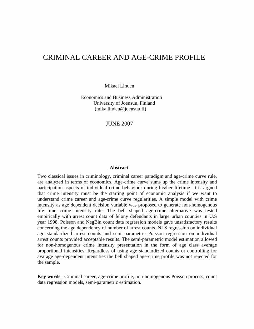
basically tell the story of age dependency of crime participation. The peak is obtained age

20 but other lower peak is found at age 32. Thus the unimodality of aggregate age-crime

profile is not valid in this sample but right skewness is obvious. Next eight pictures (age

distributions of arrested in different arrest number classes) give the explanation for found

density estimate. The peak number of arrests shift toward right and the distributions

normalizes with age. Most importantly the number of arrested decreases fast with the age

and the number of arrests.

22

Figures 3-10. Age Distributions of Arrested with Different Arrest Numbers

23

Figures 11. Distribution of Number of Arrests

.00

.02

.04

.06

.08

.10

.12

.14

0 10 20 30 40 50 60 70 80 90 100 110

NUMBER OF ARREST

Density Estimate of Number of Arrests

Figure 11 shows that arrest number declines rapidly after the first arrest in sample. The

distributions are similar in all age classes (see Appendix IV). Thus shape of relative

crime frequency in different age classes remains same but the number of arrested

participation) is lower in higher age classes. Finally Box –plots in Figures 12 and 13 sum

the information above. Figure 12 shows the distributions of number of arrests at different

ages. Figure 13 tells the story in the opposite way: the age distributions of given arrest

numbers.

Age class crime intensity distributions in Figure 12 are clearly skewed, mean values

increase with the age, and in age classes above 57 years distributions are very diffuse.

However after age 45 the increase ceases. The number of defendants is low in higher age

classes due the voluntary and involuntary drop-out selection of crime careers. The Box-

plots in Figure 13 confirm us the earlier results that crime intensity increases with age but

many outliers are found with arrest number less than 20. Age distributions with high

arrest numbers are also very diffuse. Expected age of defendants increase with number of

arrest when number of arrests is below 25 but after that it seems to decline or stabilize.

24

Figure 12. Distributions of Number of Arrests in Age Classes

-10

0

10

20

30

40

50

60

70

13 17 21 25 29 33 37 41 45 49 53 57 61 65 69 74 78

NUM

BER O

F ARRESTS

AGE

Figure 13. Distribution of Number of Arrests

-20

0

20

40

60

80

100

120

1 5 9 13 17 21 25 29 33 37 41 45 49 53 57 61 65 69 77 89

AG

E

NUMBER OF ARRESTS

Generally the figures support the view that inverted U-shape age-crime profile is valid in

analyzed sample but tail behaviour of marginal distributions of two-dimensional age and

arrest number distribution are diffuse (see also Figure 14). This makes the conditional

25

modeling of number of arrests with given age of arrested, i.e. [ | ]E Y X age= , a

demanding task.

Figure 14. Age and number of arrests in 3D

AGE and NUMBER OF ARRESTS

2517

80

30

25

20

15

220

165

110

55

0

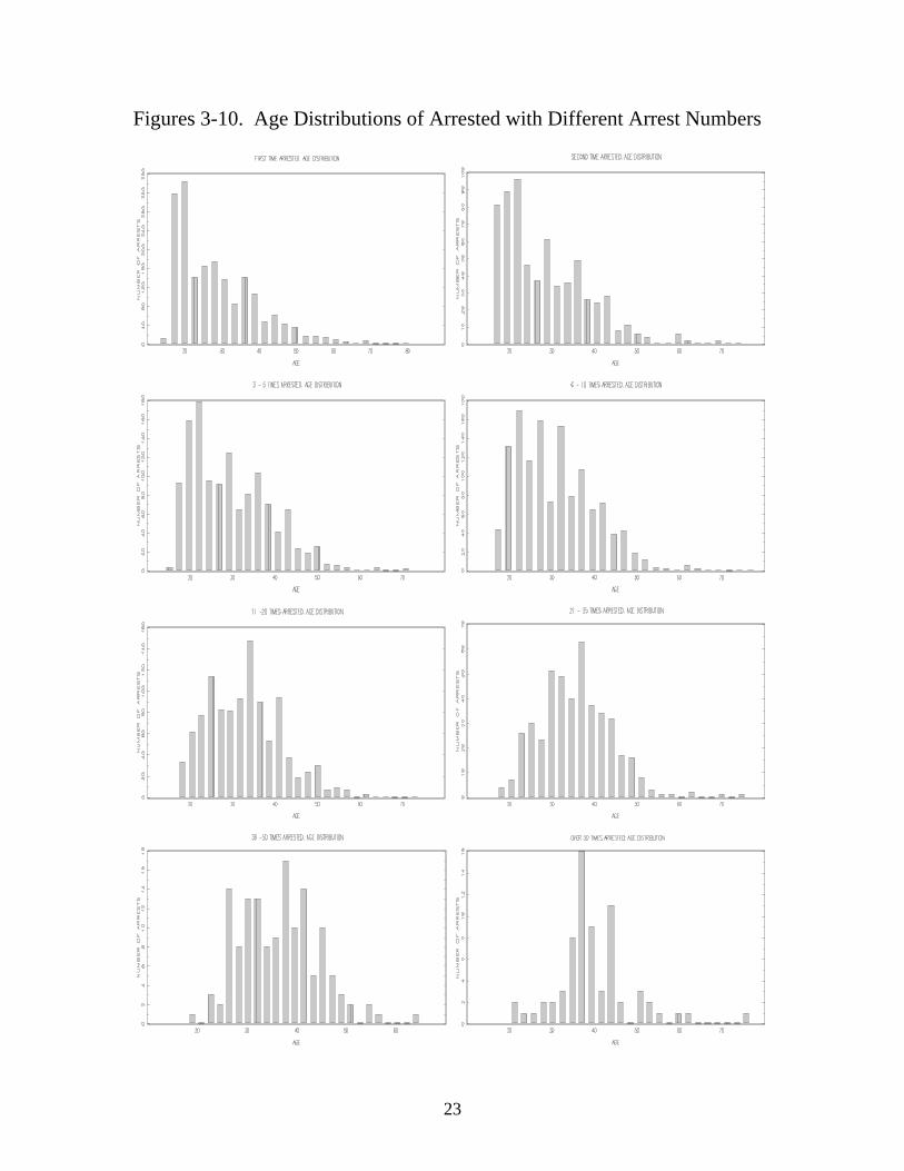
V. Estimation results We first report least square estimation results on age standardized intensities /i iTλ .

Figure 15. below depicts the age distribution of /i Tiλ (see also Appendix V). We notice

that age response to /i Tiλ gives the age-crime profile shape. In Figure 15 number of

arrested per age increases faster than age under age class 27 and after it the converse

happens. The increasing mean intensity values are in accordance with Leung’s

assumption of increasing age-crime intensity. The OLS estimation with different

26

Figure 15. Age and age standardized crime counts

-0.2

0.0

0.2

0.4

0.6

0.8

1.0

13 17 21 25 29 33 37 41 45 49 53 57 61 65 69 74 78

NU

MB

ER

OF

AR

RE

STS

/ AG

E

AGE

covariates show that negative age effects dominates in multivariate regression setting.

Number of prior convictions (PRICONV) does not halter age standardized number of

arrested. Prior prison and jail incarcerations (PRIJAIL, PRIPRIS) do not affect them in

statistically significant way. However the severity of prior arrests (SERARR) increases

standardized arrests and prior convictions effects are non-significant. Non-white males

are most often arrested and larger the state (city) less arrests happen. NLS –estimation of

Poisson type model with 20 1 2( )i i iF T a a T Tα= + + on age standardized arrest counts are

close to OLS estimation results. Note negative corresponds to bell shaped age-crime

profile hypothesis. However the coefficient estimates of PRIJAIL, PRIPRIS, and STATE

lose their statistical significance. Coefficient for SERCONV turns positive and is

statistically significant.

2a

27

Table 3. OLS on PRIARRG = arrests/age: 0 1/i i iT T iλ α α ε= + + +ix 'β

Method: Least Squares, N = 6827 White Heteroskedasticity-Consistent Standard Errors & Covariance

Variable Coefficient Std. Error t-Statistic Prob.

C 0.154841 0.010264 15.08573 0.0000 AGE -0.003618 0.000234 -15.47848 0.0000

PRICONV 0.043868 0.002689 16.31571 0.0000 PRIJAIL 0.004997 0.003504 1.425968 0.1539 PRIPRIS -0.004473 0.004193 -1.066720 0.2861

RACE 0.009234 0.003527 2.617997 0.0089 SERARR 0.083795 0.003423 24.47661 0.0000

SERCONV -0.005002 0.005124 -0.976094 0.3291 SEX -0.034881 0.004407 -7.915146 0.0000

STATE -0.002290 0.000310 -7.382945 0.0000

R-squared 0.605303 Mean dependent var 0.229880 Adjusted R-squared 0.604782 S.D. dependent var 0.315579 S.E. of regression 0.198393 Akaike info criterion -0.395666

Table 4. NLS on PRIARR =arrests/age: 2

0 1 2/ exp[ ]i i i i iT a a T Tλ α ε= + + + +ix 'β

Method: Non-Linear Least Squares, N = 6827 White Heteroskedasticity-Consistent Standard Errors & Covariance ================== ======== ========== ========== ========

Coefficient Std. Error t-Statistic Prob.

C -4.760519 0.227273 -20.94628 0.0000 AGE 0.026478 0.012039 2.199385 0.0279

AGE2 -0.000617 0.000181 -3.410445 0.0007 PRICONV 0.046751 0.006835 6.840137 0.0000 PRIJAIL 0.005105 0.007384 0.691324 0.4894 PRIPRIS 0.009112 0.013265 0.686907 0.4922

RACE 0.073747 0.027966 2.637073 0.0084 SERARR 1.023955 0.041260 24.81730 0.0000

SERCONV 0.217287 0.023041 9.430374 0.0000 SEX -0.176210 0.043011 -4.096840 0.0000

STATE -0.002308 0.002339 -0.986915 0.3237

R-squared 0.534479 Mean dependent var 0.229880 Adjusted R-squared 0.533796 S.D. dependent var 0.315579 S.E. of regression 0.215475 Akaike info criterion -0.230334

28

Table 5. MLE with Poisson model on PRIARR =arrests 2

0 1 2exp[ln ]i i iT a a Tλ α= + +i+ x 'β iT+

Dependent Variable: PRIARR, N = 6827 Method: ML/QML - Poisson Count (Quadratic hill climbing) QML (Huber/White) standard errors & covariance

Variable Coefficient Std. Error z-Statistic Prob.

ln(AGE) 1.00 C -5.226 0.168 -32.30 0.000

AGE -0.0038 0.0081 -0.478 0.636 AGE2 -0.00017 0.00011 -1.578 0.115

PRICONV 0.0637 0.0072 8.851 0.000 PRIJAIL 0.0015 0.0075 0.206 0.836

PRIPRIS -0.0007 0.0125 -0.062 0.951 RACE 0.050 0.0210 2.365 0.018

SERARR 1.365 0.0352 38.31 0.000 SERCONV 1.188 0.0244 7.731 0.000

SEX -0.209 0.0331 -6.031 0.000 STATE -0.0082 0.0018 -4.476 0.000

R-squared - Mean dependent var 7.222 Adjusted R-squared - S.D. dependent var 10.497

Log likelihood -20561.27 Restr. log likelihood -48103.79Test of restriction θ =1

for θ ln(AGE) 98.55 (p-value: 0.00) Over-dispersion test 13.03 (0.00)

Katz-family test 23.51 (0.00) Test against NegBin 998.2 (0.00)

Results of ML–estimation of Poisson and Negative Binomial regression models with

restriction 1θ = against the alternative 1θ > are confusing. The coefficient values and

their statistical significances do not conflict the results for NLS–estimation but age

variables (AGE and AGE2) get non-significant or opposite results compared to OLS/NLS

–estimation rejecting the age-crime profile hypothesis. Over-dispersion and Katz family

tests reject the Poisson alternative. Also the test against NegBin –alternative is rejected.

However Vuong test favors Poisson model against NegBin -alternative with Normal

unobserved heterogeneity with test value of -16.11 (see the likelihood values). Evidently

29

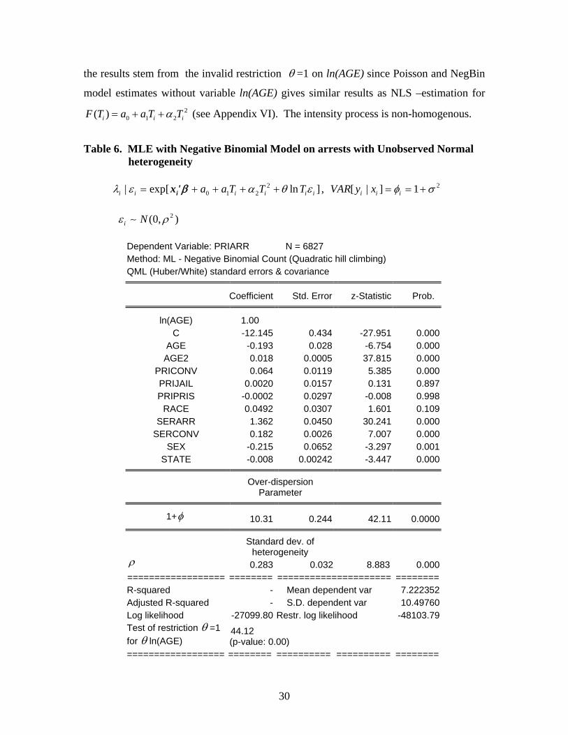
the results stem from the invalid restriction θ =1 on ln(AGE) since Poisson and NegBin

model estimates without variable ln(AGE) gives similar results as NLS –estimation for 2

0 1 2( )i i iF T a a T Tα= + + (see Appendix VI). The intensity process is non-homogenous.

Table 6. MLE with Negative Binomial Model on arrests with Unobserved Normal heterogeneity 2

0 1 2| exp[ ln ]i i i i i ia a T T Tλ ε α θ ε= + + + +ix 'β 2[ | ] 1i i iy x, VAR φ σ= + = 2(0, )i Nε ρ∼

Dependent Variable: PRIARR N = 6827 Method: ML - Negative Binomial Count (Quadratic hill climbing) QML (Huber/White) standard errors & covariance

Coefficient Std. Error z-Statistic Prob.

ln(AGE) 1.00 C -12.145 0.434 -27.951 0.000

AGE -0.193 0.028 -6.754 0.000 AGE2 0.018 0.0005 37.815 0.000

PRICONV 0.064 0.0119 5.385 0.000 PRIJAIL 0.0020 0.0157 0.131 0.897 PRIPRIS -0.0002 0.0297 -0.008 0.998

RACE 0.0492 0.0307 1.601 0.109 SERARR 1.362 0.0450 30.241 0.000

SERCONV 0.182 0.0026 7.007 0.000 SEX -0.215 0.0652 -3.297 0.001

STATE -0.008 0.00242 -3.447 0.000

Over-dispersion

Parameter

1+φ 10.31 0.244 42.11 0.0000

Standard dev. of

heterogeneity ρ 0.283 0.032 8.883 0.000 ================== ======== ===================== ======== R-squared - Mean dependent var 7.222352 Adjusted R-squared - S.D. dependent var 10.49760 Log likelihood -27099.80 Restr. log likelihood -48103.79 Test of restriction θ =1 for θ ln(AGE)

44.12 (p-value: 0.00)

================== ======== ========== ========== ========

30

Results with semiparametric proportional cumulative intensity function are reasonable.

The estimation is conducted for age classes 13 – 56 since above age class 56 the

intensities are very unstable (see Figure 13 or 15). We lose 98 observations of full sample

(1.4% of sample) due to the truncation. Most important finding, compared to earlier

results, is the semi-parametric estimate for that controls much of variability of age

class dependent intensity (see Figure 16). The outcome is more transparent when non-

cumulative intensities are depicted (see Figures 17a and 17b). The semiparametric

presentation is much less in scale and flatter than the non-parametric data estimate for

cumulative intensity (

0ˆ ( )tΛ

*( )tλ

=β 0 ).

Table 7. MLE with Semiparametric Proportional Cumulative Intensity

1

1* 10 ˆ ˆ' '

1

( ) ( ) ( ) ( )ˆ ( ) i i

l li

i

in n i

m mn

l n l i

n T n T n t n Tte e

−− −

== =

− −Λ = +∑∑ ∑x xβ β

Dependent Variable: PRIARR N = 6729 AGE CLASSES

13 – 56 Method: ML (Newton-Raphson ) White Heteroskedasticity-Consistent Standard Errors & Covariance

Coefficient Std. Error z-Statistic Prob.

AGE 0.0342 0.0022 15.59 0.000 AGE2 -0.0004 0.00003 -13.61 0.000

PRICONV 0.066 0.0009 71.032 0.000 PRIJAIL 0.0007 0.0004 1.787 0.043 PRIPRIS -0.0045 0.0007 -6.037 0.000

RACE 0.0380 0.0080 4.728 0.000 SERARR 1.3390 0.0115 116.422 0.000

SERCONV 0.1792 0.0061 29.157 0.000 SEX -0.2232 0.0060 -36.947 0.000

STATE -0.0082 0.0004 -20.627 0.000

R-squared - Mean dependent var 7.2239Log likelihood -12431.32 S.D. dependent var 10.4636================= ======== ========== ========== ========

31

Note that construction of Poisson model with semiparametric intensity assumed that

model does not include a constant term. Every age class a specific constant term, that is

or for , although all classes share the same parametric

presentation for crime counts.

0ˆ ( )tΛ *( )tλ 1 20 .... mT T T< ≤ ≤ ≤

The results imply that the age-crime profile in still bell shaped when estimation controls

both for individual and average age class intensity effects. The result does not support

Leung’s conjecture of increasing intensity with age. The results are more in line with

model implications derived earlier in the paper: both the crime intensity and participation

are decreasing with age. Note that we have not provided 95% confidence intervals for

average age intensity estimates. Anyway we have succeeded to separate age class

dependent intensities and individual control effects on crime counts. The semiparametric

estimation provides more precise estimates than alternative models since the non-

homogenous intensity presentation is also estimated in the presence of the individual

controls, including age, for the counts.

Figure. 16. Cumulative proportional intensities

5753484439353126221713

AGE

350

315

280

245

210

175

140

105

70

35

0

CU

MU

LATI

VE

INTE

NS

ITY

CUMULATIVE INTENSITY FUNCTIONS

Legend

CUMULATIVE INTENSITY (MLE)CUMULATIVE INTENSITY (b=0)

32

Figure 17a. Age class average intensities

5753484439353126221713

AGE

14

13

11

10

8

7

6

4

3

1

0

INTE

NS

ITY

INTENSITY (b=0)

Figure 17b. Semiparametric average age class intensities

5753484439353126221713

AGE

2.0

1.8

1.7

1.5

1.4

1.2

1.0

0.9

0.7

0.6

0.4

INTE

NS

ITY

INTENSITY (MLE)

33

VI. Conclusions Two classical issues in criminology, criminal career paradigm and age-crime curve (or

profile) rule, were re-opened into analysis with economic analysis. Although age-crime

curve and criminal career (or recidivism) are conceptually distinct they are closely

interlinked empirically to each other. The career paradigm can’t be put aside when

analyzed data contains individuals with repeated arrests. Age-crime curve and profile

sum up the crime intensity and participation aspects of individual crime behaviour during

his/her lifetime. The age dependency is relevant for both the intensity and the

participation. The latter is typically considered to produce the observed age-crime curve

as the repeated criminal activity calms down voluntary or involuntary after age of 25.

However this answer is too simple, and partly wrong, since observed individual criminal

intensity, e.g. number of crimes per year, varies substantially also with age. We have

tried argue like Leung (1994) that crime intensity must be the starting point of the proper

analysis, since if want to understand crime career and age-crime curve regularities with

economic terms, the whole crime career is the exposition time during the crimes are

committed. Thus the economic modeling takes the crime intensity as age dependent

decision variable where both the number of crimes and the length of crime career

generate non-homogenous intensity rate.

A simple model that included the salient features of crime career and age-crime curve

was proposed. It was assumed that individuals can control their crime intensity. The

criminal sets his crime intensity rate at level that minimizes his expected time devoted to

criminal activity incurring some costs. By augmenting the basic model with fixed

expected life time during the optimal number of crimes can be committed we were able

to show that increased number of crimes increases the expected life time. The result gives

an explanation to question why old criminals necessarily do not commit less crime per

their age compared to young criminals. Thus their intensity rate can still be high but the

number of old criminals is less among the total number of criminals due the participation

selection effect. The assumption of age dependent subjective time preference and

34

shortening remaining life emphasize the model results where crimes are committed at the

beginning of life time.

In the empirical part of study the arrests count data of felony defendants in large urban

counties in U.S in year 1998 was analyzed with count-data regression methods. It was

shown that Poisson and NegBin models give unsatisfactory results concerning the age

dependency of number of arrest counts as the models are based on constant intensity

rate. Much better results were obtained with NLS–method on individual age standardized

counts, and with semi-parametric Poisson estimation on individual arrest counts where

average age class effects are controlled for age dependency of crime intensity. The

estimates of parametric part of models showed that sex, race, and past criminal record

and its seriousness had the typical, and too often observed, influences on crime counts.

Only the number of prior prison incarcerations reduced the number of arrests.

The parametric part of models also included the individual age effect function 2

0 1 2( )i i if T a a T Tα= + + . The function tested the bell shaped age-crime profile hypothesis

in the presence of age standardized and non-standardized counts, i.e. life time intensities.

The age function estimates indicated that the average age-crime profile is still a bell

shaped in the sample although we control for average class intensities in semi-parametric

model and NLS –approach is based on age standardized arrest counts. The results

rejected the Leung (1994) approach where crime intensity increases with age but

confirmed some of our model predictions. In general the results support the view the

age-crime curve is still alive and well.

35

APPENDIX I

0

1 * 1

0

21

02

2

* 02

[ ] (1 ) [ ] 0

( ) 0 : ,

[ ]where 0 and (1 )

[ ] (1 ) [ ] and

[ ] | (1 ) [ ] ( 1)S S

dE kE T t S SdS

g S S B S B

E TBkt

d E kE T t SdS

d E kE T t BdS

α α

α α

α

α α

α 0.

τ α μ β

βα μ

τ α α μ β

τ α α μ β α β

−

− −

− −

−=

= + − =

⇒

= − = =

= >+

= + −

= + − = − >

APPENDIX II 1

0 [ ] 0, where (1 ) >0. AE T S A ktα α β α μ− − − = = +

Differencing totally this first order condition with respect to [ ] and E T S

2 1 11 2

2 1 11 2

1

2

[ ] ( 1) [ ] [ ] [ ] 0,

where [ ] ( 1) >0 and [ ] 0

[ ] [ ]( 1) 1 [ ] 0 : .[ ] [ ] 1 1

AE T S dS AS E T dE T A dS A dE T

A AE T S A AS E T

AdE T E T E T dS S v vdS A S v S dE T E T

α α α α

α α α α

α α

α α

α αα α α α

− − − − −

− − − − −

− − = − =

= − = >

−⇒ = = = − > = =

− −α

>

Next we analyze the sign of [ ] /dE T dμ . -1

0 [ ] 0, where (1 ) 0. CE T C kt Sα αμ β α− − = = + > Differencing totally this first order condition with respect to [ ] and E T μ

36

11 2

11 2

1

2

[ ] [ ] [ ] [ ] 0,

where [ ] 0 and [ ] 0

[ ] 0.

CE T d C E T dE T C d C dE T

C CE T C C E T

CdE Td C

α α

α α

μ μα μ

μα

μ

− − −

− −

− = −

= > = >

⇒ = >

−

=

>

t

Results for are obtained in similar way. 0[ ] / 0 and [ ] / 0 dE T dk dE T dt> APPENDIX III The discounted expected life time, when * *t T= − is the planned remaining life time, is

( *) ( *) ( *)

0

1 1[ | ] [ [1 ]]tr t r t x r t

te E T t e e dx ee

φφφ

− − − −< ∞ = = −∫ .

Differencing this with respect to t we obtain

( * ) ( * ) ( * )

( * )

1 1 [ [ (1 )]] [ '( ) (1 ) ]

1 [ '( )(1 )] .

r T t t r T t t r T t t

r T t t t

d e e r t e e e e dt

e e r t e dt

φ φ

φ φ

φφ φ

φφ

− − − − − − − − −

− − − −

− = − +

= + −

φ

tφ−

<

The function alters its sign from positive to negative with a value

( ) '( )(1 )tg t e r t eφφ −= + −(0, *), when * and '( ) 0.t T T r t∈ → ∞

For example with 2

2( ) br t at t= − we obtain ( ) [ ] tg t a bt e btφφ −= − + − where (0) 0 g aφ= − > and . ( )g ∞ = −∞

Now, if 0.5, 0.05, and 0.005a bφ = = = , then ( 5.7)g t 0= ≈ .

37

APPENDIX IV Number of Arrest in Different Age Classes

38

APPENDIX V INTENSITY OF CRIME IN DIFFERENT AGE CLASSES Descriptive Statistics for PRIARRG = arrests/age Categorized by values of AGE Included observations: 6827

AGE Mean Std. Dev. Obs.13 0.000000 NA 114 0.047619 0.082479 315 0.024242 0.080403 1116 0.045673 0.102405 2617 0.072591 0.184902 14118 0.104238 0.227648 38819 0.147569 0.197732 36720 0.198899 0.351168 31821 0.179539 0.236061 28322 0.229521 0.284370 28323 0.229865 0.296120 24424 0.257037 0.362554 22525 0.240637 0.279519 25126 0.290617 0.344655 23227 0.299121 0.400833 23628 0.252723 0.335130 22329 0.222257 0.280762 22030 0.304538 0.396268 21331 0.258065 0.285191 21132 0.292271 0.326247 22433 0.268328 0.322297 24834 0.287701 0.310741 22035 0.263172 0.367075 21836 0.295930 0.409346 20237 0.277443 0.335962 21138 0.260249 0.342393 19039 0.251792 0.332567 16140 0.257292 0.296251 16841 0.246377 0.294197 13842 0.288132 0.342016 12843 0.196549 0.274324 12444 0.291924 0.421032 10345 0.247737 0.329405 8146 0.216498 0.288776 7347 0.256714 0.269882 6148 0.178066 0.212285 5349 0.182982 0.226590 5950 0.250980 0.362642 51

39

51 0.153251 0.227062 3852 0.187965 0.272766 3153 0.152740 0.262590 2154 0.125220 0.155589 2155 0.234091 0.332475 1656 0.199176 0.212398 1357 0.008772 0.017544 458 0.064655 0.105380 859 0.096852 0.245385 1460 0.018333 0.041907 1061 0.081967 0.117359 962 0.232719 0.443461 763 0.142857 0.127644 764 0.113281 0.138217 465 0.125641 0.235021 666 0.136364 0.064282 267 0.007463 0.010554 268 0.000000 NA 169 0.032609 0.055974 470 0.069048 0.162234 671 0.018779 0.021514 372 0.027778 NA 174 0.114865 0.162443 275 0.060000 0.065997 276 0.289474 NA 177 0.805195 NA 178 0.089744 NA 180 0.000000 NA 181 0.000000 0.000000 2All 0.229880 0.315579 6827

40

APPENDIX VI Dependent Variable: PRIARR, N = 6827 Method: ML/QML - Poisson Count (Quadratic hill climbing) QML (Huber/White) standard errors & covariance

Variable Coefficient Std. Error z-Statistic Prob.

C -3.206763 0.169363 -18.93422 0.0000AGE 0.052705 0.008837 5.964434 0.0000AGE2 -0.000552 0.000126 -4.391824 0.0000

PRICONV 0.063757 0.007224 8.825754 0.0000PRIJAIL 0.001482 0.007544 0.196398 0.8443PRIPRIS -0.000899 0.012658 -0.071042 0.9434

RACE 0.050533 0.021287 2.373937 0.0176SERARR 1.366285 0.035650 38.32450 0.0000

SERCONV 0.190435 0.024506 7.770815 0.0000SEX -0.207850 0.033163 -6.267530 0.0000

STATE -0.008206 0.001856 -4.420355 0.0000

Log likelihood -20595.94Restr. log likelihood -48103.79

Method: ML - Negative Binomial Count (Quadratic hill climbing) QML (Huber/White) standard errors & covariance

Coefficient Std. Error z-Statistic Prob.

C -3.496442 0.131476 -26.59382 0.0000AGE 0.050857 0.006418 7.923781 0.0000

AGE2 -0.000561 8.85E-05 -6.337929 0.0000PRICONV 0.107470 0.005979 17.97500 0.0000PRIJAIL 0.010028 0.007565 1.325617 0.1850PRIPRIS -0.041233 0.008709 -4.734323 0.0000

RACE 0.026668 0.019696 1.353952 0.1758SERARR 1.485725 0.032041 46.36942 0.0000

SERCONV 0.099808 0.024841 4.017896 0.0001SEX -0.222625 0.032523 -6.845219 0.0000

STATE -0.008750 0.001758 -4.978525 0.0000

Mixture Parameter

1+φ 1 + 0.356 0.315 11.520 0.0000

Log likelihood -15170.91Restr. log likelihood -48103.79

41

References Adda, J. & Cooper, R. (2003) Dynamic Economics, MIT Press. Berkovic, J. & Stern, S. (1991) “Job Exit Behaviour of Older Men”, Econometrica 59, 189-210. BJS (Bureau of Justice Statistics) (1998) “Felony Defendants in Large Urban Counties USA, 1998”, State Court Processing Statistics. U.S. Dept. of Justice. Blumstein, A. (2005) “An Overview of the Symposium and Some Next Steps”, Annals of the American Academy of Political and Social Science 602, 242-258. Blumstein, A. & Cohen, J. (1979) “Estimation of Individual Crime Rates from Arrested Records”, Journal of Criminal Law and Criminology 70, 561-585. Campbell, A. (1995) “A Few Good Men - Evolutionary Psychology and Female Adolescent Aggression”, Ethology and Sociobiology 16, 99-123. Davis, M.L. (1988) “Time and Punishment: An Intertemporal Model of Crime”, Journal of Political Economy 96, 383-390. D’Unger, A.V., Land, K.C. & McCall, P.L. (2002) “Sex Differences in Age Patters of Delinquent/Criminal Careers: Results from Poisson Latent Class Analyses of Philadelphia Cohort Study ”, Journal of Quantitative Criminology 18, 349-375. Fagan, A.A. & Western, J. (2005) “ Escalation and Deceleration of Offending Behaviours from Adolescence to Early Adulthood”, Australian and New Zealand Journal of Criminalogy 38, 59-76. Gottfredson, M. & Hirschi, T. (1990) A General Theory of Crime, Stanford UP. __________________ (1983) ”Age and the Explanation of Crime” American Journal of Sociology 96, 552-584. Heineke, J.M. (1978) “Economic Models of Criminal Behaviour: An Overview” in Economic Models of Criminal Behaviour, J.M. Heineke (ed.), North-Holland. Hopenhayen, H. & Rogerson, R. (1993) “Job Turnover and Policy Evaluation: A General Equilibrium Analysis”, Journal of Political Economy 101, 915-38. Jacob, B., Lefgren, L. & Moretti, E. (2004) “The Dynamics of Criminal Behaviour: Evidence from Weather Shocks”, NBER-WP 10739. Kanazawa, S. (2002) “Why Productivity Fades with Age: The Crime-Genius Connection”, Journal of Research in Personality 37, 257-272. Kyvsgaard, B. (2003) The Criminal Career. The Danish Longitudinal Study. Cambridge University Press. Land, K.C. (1992) “Models of Criminal Careers: Some Suggestions for Moving Beyond the Current Debate”, Criminology 30, 149-155. Lawless, J.F. (1987) “Regression Methods for Poisson Process Data”, JASA 82, 808-815. Lee, D.S. & McCrary, J. (2005) “Crime, Punishment, and Myopia”, NBER-WP 11491. Leung, S. F. (1995) “Dynamic Deterrence Theory”, Economica 62, 65-87. _________ (1994) “An Economic Analysis of the Age-Crime Profile”, Journal of Economic Dynamics and Control 18, 481-497. _________ (1991) “How to Make the Fine Fit the Corporate Crime? An Analysis of Static and Dynamic Punishment Theories”, Journal of Public Economy 45, 243-256. Levitt, S.T. (1999) “The Limited Role of Changing Age Structure in Explaining Aggregate Crime Rates”, Criminology 37, 581-605.

42

Nagin, D.S. & Land, K.C. (1993) “Age, Criminal Careers, and Population Heterogeneity: Specification and Estimation of a Nonparametric, Mixed Poisson Model”, Criminology 31, 327-362. Polinsky, A.M. & Rubinfield, R. (1991) “A Model of Optimal Fines for Repeat Offenders”, Journal of Public Economy 46, 291-306. Rust, J. (1996) “Numerical Dynamic Programming in Economics” in Handbook of Computational Economics Vol. I, 619-729. North-Holland.

43