This is a repository copy of Endogeneity Bias in Marketing Research: Problem, Causes and Remedies.

White Rose Research Online URL for this paper:http://eprints.whiterose.ac.uk/116923/

Version: Accepted Version

Article:

Zaefarian, G orcid.org/0000-0001-5824-8445, Kadile, V orcid.org/0000-0001-9266-3861, Henneberg, SC et al. (1 more author) (2017) Endogeneity Bias in Marketing Research: Problem, Causes and Remedies. Industrial Marketing Management, 65. pp. 39-46. ISSN 0019-8501

https://doi.org/10.1016/j.indmarman.2017.05.006

© 2017 Elsevier Inc. This manuscript version is made available under the CC-BY-NC-ND 4.0 license http://creativecommons.org/licenses/by-nc-nd/4.0/

eprints@whiterose.ac.ukhttps://eprints.whiterose.ac.uk/

Reuse

Items deposited in White Rose Research Online are protected by copyright, with all rights reserved unless indicated otherwise. They may be downloaded and/or printed for private study, or other acts as permitted by national copyright laws. The publisher or other rights holders may allow further reproduction and re-use of the full text version. This is indicated by the licence information on the White Rose Research Online record for the item.

Takedown

If you consider content in White Rose Research Online to be in breach of UK law, please notify us by emailing eprints@whiterose.ac.uk including the URL of the record and the reason for the withdrawal request.

1

Endogeneity Bias in Marketing Research: Problem, Causes and Remedies

Ghasem Zaefarian * Lecturer in Marketing

University of Leeds, Leeds University Business School, Maurice Keyworth Building, Leeds LS2 9JT, United Kingdom

Telephone: +44 (0)113 343 3233 Email: G.Zaefarian@leeds.ac.uk

Vita Kadile

Research Fellow in Marketing University of Leeds, Leeds University Business School

Maurice Keyworth Building, Leeds LS2 9JT, United Kingdom Telephone: +44 (0) 113 343 3217

Email: V.Kadile@leeds.ac.uk

Stephan C. Henneberg

Professor of Marketing and Strategy Queen Mary University of London, School of Business and Management, Business

Ecosystems Research Group London E1 4NS, United Kingdom Telephone: +44 (0)207 882 6544 Email: S.Henneberg@qmul.ac.uk

Alexander Leischnig

Professor of Marketing Intelligence University of Bamberg

Feldkirchenstraße 21, 96052 Bamberg, Germany Telephone: +49 (0)951 863 2970

Email: Alexander.Leischnig@uni-bamberg.de

Submitted to Industrial Marketing Management: November 15, 2016

First revision: March 9, 2017

Second revision: May 12 2017

Accepted: May 24, 2017

Acknowedgement

The authors would like to thank Peter LaPlaca and Matthew Robson for encouraging us to write

about the topic of endogeneity as well as Peter Naudé for his suggestions and help with the

manuscript.

* Corresponding author

2

Endogeneity Bias in Marketing Research: Problem, Causes and Remedies

Abstract

Endogeneity bias represents a critical issue for the analysis of cause and effect

relationships. Although the existence of endogeneity can produce severely biased results, it has

hitherto received only limited attention from researchers in marketing and related disciplines.

Thus, this article aims to sensitize researchers intending to publish in the Industrial Marketing

Management (IMM) journal to the topic of endogeneity. It outlines the problem of endogeneity

bias, and provides an overview of potential sources, i.e. omission of variables, errors-in-

variables, and simultaneous causality. Furthermore, the article shows ways to deal with

endogeneity, including techniques based on instrumental variables as well as instrument-free

approaches. Our methodological contribution relates to providing researchers aiming to publish

in IMM with an initial overview of the causes of and remedies for endogeneity bias, which

should be considered in designing research projects as well as when analysing data to obtain

insights into cause and effect relationships (causal models).

3

1. Introduction

An increasing number of articles in marketing as well as in related fields such as

international business, supply chain management, and operations management have recently

pointed to issues associated with endogeneity (Guide & Ketokivi, 2015; Jean, Deng, Kim, &

Yuan, 2016; Shugan, 2004). Endogeneity constitutes a critical problem for research as it

compromises key conditions for claiming causality (Antonakis, Bendahan, Jacquart, & Lalive,

2010, 2014) and both the direction and the size of its bias are difficult to predict in advance

(Hamilton & Nickerson, 2003). A failure to consider and correct for endogeneity in research

practice can lead to biased and inaccurate results, and poses the risk of drawing incorrect

conclusions about cause and effect relationships between concepts of interest. Even though the

issue is much more predominant in naturally occurring data (e.g. regularly and automatically

collected customer data at the point of purchase or via web browsing) as opposed to market

research data (e.g. data collected through survey questionnaires), and is less of a problem for

experimental data (e.g. Anderson & Simester, 2004), any study involving questionnaire or

survey design is potentially subject to endogeneity bias (Toubia, Simester, Hauser, & Dahan,

2003).

Endogeneity is most commonly described in the context of ordinary least squares (OLS)

estimation, and refers to a situation in which an independent (explanatory) variable correlates

with the structural error term (also referred to as ‘disturbance term’ or ‘residual’) in a model

(Kennedy, 2008; Wooldridge, 2002). In such a situation, the error term is not random and the

estimation is inconsistent, which implies that the coefficient estimate of the independent

variable fails to converge to the true value of the coefficient in the population as sample size

increases. When an independent variable correlates with the error term, the coefficient estimate

includes the effect of the respective independent variable on the dependent variable as well as

the effects of all unobserved factors that correlate with the independent variable and explain

4

the dependent variable, thus rendering its interpretation problematic, or even useless

(Antonakis et al., 2010, 2014). If this correlation is ignored, the estimated effect of the observed

variable is likely to be biased. This bias is referred to as the endogeneity bias (Chintagunta,

Erdem, Rossi, & Wedel, 2006).

Endogeneity is a major concern in many areas of marketing and related research, which

rely on employing regression-based analyses with the aim to draw causal inferences (Jean et

al., 2016). In essence, endogeneity may affect the causal inferences that researchers make with

regard to the hypothesized associations between variables, and failure to account for this may

lead to spurious findings resulting in misleading theoretical as well as managerial implications

(Semadeni, Withers, & Certo, 2014). Against this background, editors and reviewers of various

disciplines in the area of management studies increasingly point to endogeneity as a likely

alternative explanation for results provided in manuscripts they process, and therefore

endogeneity considerations become more and more of a (contributing) reason for manuscript

rejection (e.g. Guide & Ketokivi, 2015; Larcker & Rusticus, 2010; Shugan, 2004). In spite of

the fact that several approaches to address endogeneity have been available for almost three

decades, only fairly recently have some of these remedies been applied in studies published in

marketing journals (Hamilton & Nickerson, 2003), and the number of researchers proactively

correcting for endogeneity still remains very low.

The Industrial Marketing Management (IMM) journal has made significant theoretical

and empirical contributions to the field of industrial and B2B marketing, as well as supply

chain management research. In many respects, the articles published in IMM are rigorous in

terms of method, e.g. by assessing several sources of bias such as non-response and common

method variance, and by incorporating measurement validity and reliability analyses.

However, the issue of endogeneity arguably is a blind spot that has not been sufficiently

addressed in research published in IMM to date. So far we have only found a dozen or so papers

5

published in IMM that tackle the issue of endogeneity in their empirical analyses, with the first

study being published by Streukens, Hoesel, and de Ruyter (2011). We therefore believe that

it is timely for the IMM research community to take the issue of endogeneity seriously. Hence

the objective of our paper is to sensitize researchers and introduce an outline for diagnosing

and correcting for potential endogeneity bias in marketing research. We discuss potential

sources of endogeneity and provide a brief overview of techniques available to account for it,

followed by an assessment of their robustness. These considerations ought to provide

suggestions for researchers in the field of marketing and supply chain management, and

especially for future publications in IMM that examine cause and effect relationships.

Our paper thus contributes to the existing knowledge on endogeneity in two ways. First,

we clarify the notion of endogeneity and its sources using marketing-related examples. Second,

we emphasize the importance of accounting for endogeneity in marketing studies and provide

an overview of remedies available to treat endogeneity bias. Overall, we aim at sensitizing

researchers who aim at publishing in IMM to the hitherto somewhat neglected topic of

endogeneity bias.

2. Sources of Endogeneity

Literature emphasizes three primary instances where the condition of exogeneity

becomes violated and therefore endogeneity occurs: omission of variables, errors-in-variables,

and simultaneous causality (Wooldridge, 2002). The following subsections briefly outline the

problems associated with each of these sources of endogeneity.

2.1 Omission of Variables

Endogeneity may occur due to the omission of variables in a model. Omission of

variables is usually attributable to data unavailability and can result in a violation of the

6

exogeneity assumption if the omitted variable that is associated with the dependent variable is

also correlated with any of the independent variables under investigation (Kennedy, 2008;

Wooldridge, 2002). In such a situation, the error term will be correlated and the coefficient

estimator of the independent variables will be biased. For instance, in investigating the effect

of firm resources on foreign market entry modes, other variables that may affect both firms’

resource slack and foreign market entry mode include managerial experience and market

characteristics. If such variables are omitted from the model and thus not considered in the

analysis, the variations caused by them will be captured by the error term in the model, thus

producing endogeneity problems.

A common form of omitted-variable-based endogeneity is omitting selection (e.g.

Antonakis et al., 2010; Clougherty, Duso, & Muck, 2016; Wooldridge, 2002). This problem

arises when respondents self-select into treatment and non-treatment groups based on

unobserved factors that correlate with the dependent and the independent variables under

investigation (this is also called the ‘choice problem’), which leads to a situation in which the

dependent variable is observable for different parts of the sample on a nonrandom basis

(Clougherty et al., 2016). Prior work shows that many business phenomena are subject to such

self-selection-based endogeneity as they involve organizational choices that are endogenous

and self-selected (Hamilton & Nickerson, 2003; Shaver, 1998). For example, firms may select

a particular relationship governance mechanism (e.g. formal vs. informal) to achieve a high

relationship performance with partner firms based on factors that are unobserved. These factors

may, for example, include the level of trust in the partner or the relationship phase. An analysis

that tests the effect of relationship governance mechanism on relationship performance will

most likely yield biased coefficient estimates unless self-selection is controlled for.

2.2 Errors-in-Variables

7

Besides omission of variables, a further source of endogeneity is errors-in-variables,

which refers to problems that arise when variables are imperfectly measured and their true

values remain unobserved (Wooldridge, 2002). Measurement errors result from the use of

inadequate measurement instruments to capture concepts of interest, or non-

comprehensiveness of the data collection method (Kennedy, 2008). Typical examples include

scale items being improperly adapted to the research context, wrong aggregation of constructs,

failures in survey translation, or non-reliable construct measures. In addition, missing data can

be considered as a form of measurement error (Kennedy, 2008). Errors-in-variables constitute

an issue when the variables on which data can be collected differ from the variables that

influence decisions of relevant actors (Wooldridge, 2002). Measurement error in the dependent

variable can cause biases if it is systematically related to one or more of the independent

variables under investigation; however, it will play a subordinate role if it is uncorrelated with

the independent variables and it is usually of minor relevance as it is captured by the error term

of the model. Measurement error in independent variables is considered as important and the

properties of the OLS estimation depend on particular assumptions about the measurement

error (Wooldridge, 2002). The first assumption is that the measurement error and the observed

independent variable are uncorrelated, and that the error term of the model is uncorrelated with

the actual (unobserved) and the observed independent variable. In this case, estimation yields

consistent coefficients. The second assumption, which is referred to as the ‘classical errors-in-

variables (CEV) assumption’, is that the measurement error is uncorrelated with the actual

(unobserved) independent variable, and that the error term of the model is uncorrelated with

the actual and the observed independent variable. In this case, the observed independent

variable and the measurement error are correlated and the estimation yields inconsistent

coefficient estimates: the coefficient estimate will be biased towards zero (‘attenuation bias’)

8

and the size of this bias depends on the variance of the actual independent variable relative to

the variance in the measurement error.

2.3 Simultaneous Causality

Endogeneity bias may also be caused by simultaneous causality, which occurs when

one (or more) independent variable is jointly determined with the dependent variable, i.e. when

independent variables and dependent variables simultaneously cause each other and causal

effects run reciprocally (Wooldridge, 2002). Because the error term of the model contains all

unobserved factors that influence the dependent variable and, in the presence of simultaneity,

the dependent variable influences the independent variable, the error term is also correlated

with the independent variable, thus leading to endogeneity problems. Using the example

mentioned above, the link between relationship governance mechanisms and relationship

performance may be affected by feedback loops and thus be subject to simultaneity: firms’

relationship governance mechanism may influence relationship performance, but relationship

performance may also affect the choice of firms’ relationship governance mechanism and the

decision to adapt it.

A related issue concerns simultaneity in the analysis of panel data and has been referred

to as dynamic endogeneity (Abdallah, Goergen, & O'Sullivan, 2015). Past realizations of the

dependent variable can influence current realizations of one or more of the independent

variables, thus producing endogeneity issues. For example, the current composition of a sales

team in an organization is likely to be influenced at least to some extent by its past sales

performance. Sales people who failed to achieve sales targets in the past may no longer be part

of the current team and may be replaced by new employees who are expected to perform better.

Consequently, past performance of the sales team or of sales employees (i.e. past realizations

of the dependent variable) has an impact on the current sales team composition. Thus, studying

9

the performance effect of sales team composition creates the risk of drawing the wrong

conclusions if the analysis does not consider dynamic endogeneity effects.

As the preceding discussion reveals, sources of endogeneity are manifold and have

several dimensions. It is therefore important to note that sources of endogeneity can cumulate

and that violation of the condition of exogeneity can have multiple reasons (Bascle, 2008).

Fortunately, prior work, especially in the econometrics literature, reveals a broad set of

techniques that enable researchers to address endogeneity problems. However, these remedies

are often not used, and recent editorials, e.g. in the Journal of International Business Studies

by Reeb, Sakakibara, and Mahmood (2012), or in the Journal of Operations Management by

Guide and Ketokivi (2015), as well as a study by Jean et al. (2016) reveal that many researchers

are either unaware of the matter of endogeneity, or do not know how to correct for it. The next

section will therefore outline different techniques to address endogeneity issues.

3. Addressing Endogeneity

Prior work emphasizes that even low levels of endogeneity can produce severely biased

and inconsistent results that increase the likeliness of making incorrect causal inferences

(Semadeni et al., 2014). It is therefore essential to not only uncover the sources of endogeneity

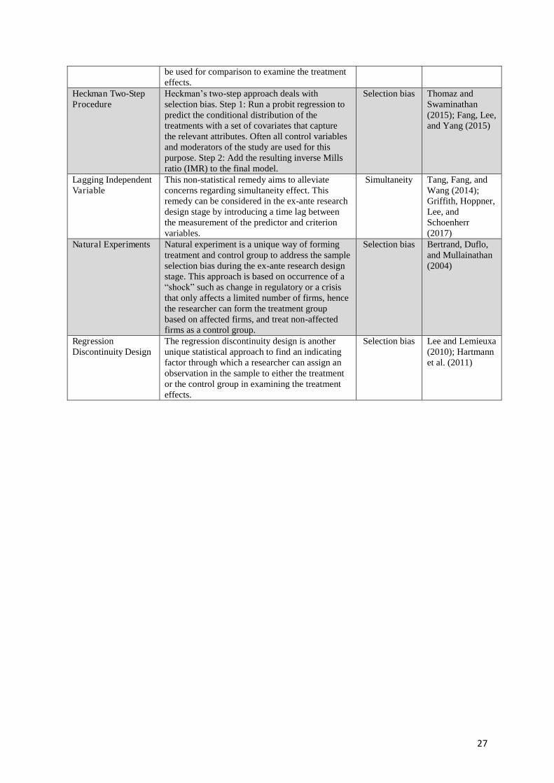
but also to take appropriate actions to address them. Table 1 gives an overview of techniques

to address endogeneity issues, which will be discussed below in greater detail.

Insert Table 1 about here

3.1 Instrumental Variables Techniques

One common approach to address endogeneity issues is the use of instrumental

variables techniques (e.g. Bascle, 2008; Semadeni et al., 2014). The basic idea behind

10

instrumental variables techniques is to decompose the variations in the endogenous

independent variable through the use of instrumental variables by focusing on the variations in

the endogenous independent variable that are uncorrelated with the error term in the model and

disregarding the variations that bias the estimation. Instrumental variables are variables that are

uncorrelated with the structural error term in a model, but which are correlated with the

endogenous independent variable, and that themselves do not represent explanatory variables

in the structural equation (i.e., the original model) (Murray, 2006). An instrumental variable

thus ‘moves around’ the endogenous independent variable, does not directly affect the

dependent variable, but affects it indirectly through the endogenous independent variable

(Rossi, 2014).

A major challenge associated with the instrumental variables techniques is to identify

valid instrumental variables. Validity of instrumental variables depends on two primary

conditions: relevance and exogeneity (Bartels, 1991; Kennedy, 2008; Murray, 2006).

Relevance refers to the degree to which an instrumental variable is sufficiently correlated with

the endogenous independent variable — with strong instrumental variables having a high

correlation and weak instrumental variables having a low correlation with the endogenous

independent variable. To assess the strength of instrumental variables, prior studies recommend

inspection of the first-stage F-statistic (of 2SLS estimation, see below) and compare the values

obtained against thresholds available in the literature (Stock, Wright, & Yogo, 2002; Stock &

Yogo, 2004). Exogeneity is defined as the degree to which an instrumental variable and the

error term in the model are uncorrelated (Murray, 2006). To assess orthogonality the Sargan

(1958) or the more general Hansen’s J-statistic (Hansen, 1982), the Basmann (1960) statistic,

and the difference-in-Sargan statistic (Hayashi, 2000) may be examined (e.g., see Bascle,

2008for further details; Murray, 2006).

11

Instrumental variables techniques may use different estimators. One of the most

commonly used instrumental variables estimators is two-stage least squares.

3.1.1 Two-Stage Least Squares (2SLS) Estimation

2SLS estimation with instrumental variables occurs in two steps. In the first, the

endogenous independent variable is regressed on the chosen instrumental variables and the

regression residual is saved. In the second step, the dependent variable is regressed on the

residual in lieu of the endogenous independent variable (Bascle, 2008; Wooldridge, 2010). An

example would be the following: let us presume one is interested in the relationship between

“Trust” and “Supplier Performance”. In this model “Trust” is the independent variable, which

is likely to be affected by omitted variables, e.g. pertaining to complex antecedent influences,

and thus endogenous, while “Supplier Performance” is the dependent variable. To address

potential endogeneity issues, 2SLS estimation may be used. First, “Trust” is regressed on the

chosen instrumental variables, say “Engagement” and “Responsiveness”, and the residual is

obtained:

Trust = b0 + b1 (Engagement) + b2 (Responsiveness) + e

Trustresidual = Trust – Trustpredicted

In this example, the chosen instrumental variables are those that have been captured

besides the substantive variables in the structural equation, and which are assumed to be

strongly correlated with the endogenous independent variable “Trust”, uncorrelated with the

dependent variable “Supplier Performance”, and do not explain the dependent variable.

Provided that the instrumental variables fulfill the conditions of relevance and exogeneity, the

second step of the 2SLS estimation replaces the endogenous independent variable “Trust” with

“Trustresidual” obtained from step one and then regresses “Supplier Performance” against

“Trustresidual”:

Supplier Performance = b0 + b1 (Trustresidual) + e

12

Whilst correcting for endogeneity using instrumental variables increases the likelihood

of reporting coefficient estimates that are near their true values, these reported estimates are

rarely statistically significant (Semadeni et al., 2014). This occurs because the most

problematic aspect of instrumental variables techniques involves the identification of valid

instrumental variables. It is imperative that in most cases one should resort to theoretical

considerations to determine whether a variable could serve as a valid instrument. However, at

times instrumental variables are selected without sufficient conceptual justification. In practice,

it remains quite difficult to identify variables that correlate strongly with the endogenous

independent variable but not with the error term in the second stage of the technique, which

makes fulfilling the essential criteria for instrument selection difficult. Nonetheless, the 2SLS

technique remains one of the most widely used methods to address endogeneity bias (Li &

Zahra, 2012; Tang & Wezel, 2015).

3.1.2 Three-Stage Least Squares (3SLS) Estimation

3SLS is another instrumental variables estimator for structural equations in which at

least one equation contains endogenous independent variables. 3SLS estimation is similar to

the 2SLS estimation, with the difference being that moderator variables are used as

instrumental variables to obtain residuals for the endogenous independent variable. Hence this

technique involves an additional third stage of regression. For example, suppose one is

interested in examining the moderating effect of “Behavioral Uncertainty” on the effect of

“Trust” on “Supplier Performance”. In this model, “Trust” is likely to be endogenous and

directly affected by the moderator “Behavioral Uncertainty”. 3SLS estimation can be used to

correct for this potential endogeneity. In the first stage, “Trust” is regressed against “Behavioral

Uncertainty” to assess the relationship between the two variables and obtain residuals for

“Trust” that exclude the effect of “Behavioral Uncertainty”. These are specified in the

following equations:

13

Trust = b0 + b1(Behavioral Uncertainty) + e

Trustresidual = Trust – Trustpredicted

In the second stage, “Supplier Performance” is regressed against “Trustresidual”. In the

third stage, an interaction term is entered into the model:

Supplier Performance = b0 + b1(Trustresidual) + c1(Trustresidual × Behavioral Uncertainty)

+ e

Note that to avoid collinearity, we need to mean center the variables before computing

the interaction term. This approach is already used in the marketing and strategy literature

(Bharadwaj, Tuli, & Bonfrer, 2011; Menguc, Auh, & Yannopoulos, 2014; Poppo, Zhou, & Li,

2016).

3.2 Instrument Free Approaches

The challenges associated with identifying valid instruments have led to alternative

approaches for correcting endogeneity, the so-called instrument-free techniques. Ebbes,

Wedel, and Böckenholt (2009) provide an extensive review of instrument free approaches used

to mitigate the concerns associated with endogeneity bias. Some of them include: the Higher

Moments (HM) approach, where instruments are built based on available data in general

regressor-error dependencies models, and can be used together with or in the absence of

traditional instruments (Erickson & Whited, 2002; Lewbel, 1997); the Identification through

Heteroscedasticity (IH) estimator, in which instruments are obtained in a similar manner to

HM, but information of heteroscedasticity is required (Hogan & Rigobon, 2003; Rigobon,

2003); and the Latent Instrumental Variables (LIV) method, whereby the variations in the

endogenous independent variable are separated into exogenous (approximated by a latent

discrete variable) and endogenous parts (Ebbes, Wedel, Böckenholt, & Steerneman, 2005). In

addition, some researchers recommend joint estimation with copulas - another instrument free

method to tackle endogeneity. A copula is a function that ‘couples’ multivariate distributions

14

to their one-dimensional marginal distribution function and captures the correlation between

the independent variable and the error term. Once this correlation is properly handled, the

model is unlikely to be affected by endogeneity problems, and estimates for model parameters

can be obtained (Park & Gupta, 2012).

Amongst instrument free approaches, many scholars prefer the application of the LIV

method (Ebbes et al., 2005; Zhang, Wedel, & Pieters, 2009), since it uses a latent variable

model to account for regressor-error dependencies, and addresses the issues of instrument

availability, weakness, and validity. The LIV estimator belongs to the family of thrifty

instruments estimators that do not require observed instruments (Ebbes et al., 2009; Ebbes et

al., 2005). Furthermore, a clear advantage of the LIV estimator is that it is a likelihood-based

approach unlike the HM and IH approaches, which belong to the family of method-of-moments

estimators. In the LIV solution, a latent variable model is used to separate the endogenous

covariate into systematic parts, whereby one part is uncorrelated with the error term and the

other part is possibly correlated with the error term. This permits achieving an unbiased

estimate of the effect of an endogenous covariate on the dependent variable. This approach was

originally developed in a linear regression setting (Rutz, Bucklin, & Sonnier, 2012) and is also

used by marketing researchers when addressing potential endogeneity bias (Zhang et al., 2009).

3.3 Matching Method

This method specifically focuses on non-random sampling issues between the treatment

and the control group. The idea is that comparison of behavioural data from firms in the sample

that did or did not exhibit certain expected outcomes are affected by selection bias. More

specifically, given the nature of business marketing research, it is nearly impossible to identify

two identical firms and allocate them into treatment and control groups, respectively, based on

the given desired outcome. For example, to study the relationship among collaborative

networks, absorptive capacity, and new product development (NPD), it is virtually impossible

15

to find collaborative networks and absorptive capacity of two identical firms, one with high

NPD performance, and one that does not practice NPD. The non-random sampling issue

explained in this example is addressed through creating a quasi-random sample.

This technique was originally developed for binary treatments (Rosenbaum & Rubin,

1983), however, it has been extended to treatments with more than two categories (Hirano &

Imbens, 2004). Using probit regressions, the matching method pairs every treatment firm with

a firm from the control group to create a quasi-control group and randomizes the data

effectively. To build this quasi-control group, a relatively large secondary dataset of control

firms is needed. For example, Chang, Chung, and Moon (2013) used some 149,000 control

firms to successfully find 1811 matched pairs of firms (statistical twins) out of their 2195

treatment groups. There are different techniques for matching statistical twins (Smith, 1997).

The matching method helps researchers to compare and contrast two statistically twinned firms

to examine the treatment effect. The propensity score matching (PSM) technique has been

widely used in recent studies (e.g. Chang et al., 2013; Garnefeld, Eggert, Helm, & Tax, 2013;

Schilke & Lumineau, 2016).

3.4 Heckman Two-Step Procedure

Heckman’s (1979) two-step procedure addresses endogeneity bias that exists in self-

selected samples. Consider the relationship between “Trust” and “Supplier Performance” as

mentioned above. It is very likely that “Trust” in a relationship with a supplier is a choice or

decision variable, i.e. managers of the buyer firm ‘choose’ to have certain levels of trust in their

relationship with a given supplier. This means that the level of “Trust” in our sample is non-

random and as such it is subject to random selection bias, which causes endogeneity. To address

this endogeneity bias, Heckman (1979) developed a two-step procedure that corrects for this

bias. In the first step of this approach, a probit regression is run to model the conditional

distribution of the treatment with a set of covariates that captures the relevant attributes. The

16

relevance of the chosen set of covariates needs to be theoretically justified. To predict the

propensity scores, some recent studies used all control variables as well as the moderators in

their model (e.g. Schilke & Lumineau, 2016). This procedure needs to be repeated for each

treatment (i.e. independent variable) of the model. In a second step, the self-selection bias is

corrected by including the resulting inverse Mills ratios (IMR) into the final regression models

before testing hypotheses. Alternatively, to assess whether endogeneity biases the results, the

main dependent variable can be regressed on the obtained propensity scores as well as the

predictors and the significant pattern1 can be compared against a rival model wherein the

propensity scores are excluded. If the overall pattern of significance remains the same in the

two models, it can be safely concluded that endogeneity is not a potential threat to the results.

The Heckman’s two-step approach has been commonly used in marketing and

management research (Heide, Kumar, & Wathne, 2014; Schilke & Lumineau, 2016; Thomaz

& Swaminathan, 2015; Verhoef, 2003). However, this approach, despite being useful and

popular among researchers, has some limitations. For example, at least one variable with a non-

zero coefficient in the selection equation in step one should not be included in the final equation

in step two. This variable essentially plays the role of an instrument, which is often not easy to

find or justify, specifically in business marketing research. Furthermore, given that this

approach aims to address selection bias, the first step of Heckman’s technique formulates a

probit model to predict the probability of selection, hence the ‘choice’ variable, i.e. the

predictor needs to be a dummy variable that takes the value of 1 if the treatment is selected,

and 0 otherwise. To overcome this limitation, one solution is to recode the predictor variable

1 To explain the significant pattern further, note that the main model is the focal conceptual model of the study that typically consists of a set of independent variables and perhaps some interaction terms, which are linked to the main dependent variable. The rival model is the same as the main model, with the addition of the correction term residual variable (as such the rival model has one additional variable). If those independent variables and interactions terms that were significant in the main model remain significant in the rival model, and the additional residual variable is not significant, then one can conclude that endogeneity is not an issue.

17

into a dummy one (e.g. Schilke & Lumineau, 2016). Alternatively, Garen (1984) provides

another two-step approach for selectivity-bias correction with a continuous choice variable

(e.g. Robson, Katsikeas, & Bello, 2008).

In the example of trust and supplier performance used above, one would need to regress

trust against a set of factors (such as firm and industry characteristics) that affect trust. The

output from this regression model may predict that a buyer firm with a given set of attributes

is more likely to have trust in the relationship with the focal supplier. In practice, researchers

often include all the control variables, independent constructs, and moderators except for the

main dependent variable(s) into the correction regression model to predict the choice variable.

Then, in the second step, they add the predicted errors from this correction regression equation

into the second-stage performance equation.

3.5 Lagging Independent Variable

Endogeneity due to simultaneity or reversed causality can also be tackled by using the

lagged endogenous regressor technique. A temporal separation through introducing a time lag

between the independent and dependent variables can reduce this bias. Given the example of

collaborative networks and NPD mentioned above, it is likely that there exists a simultaneity

effect between the two. Measuring collaborative networks in year t-1 and NPD in year t (i.e.

the dependent variable is measured in a time-lagged fashion) can significantly alleviate the

endogeneity concern stemming from simultaneity effects. However, this approach comes with

its own limitations. For example, one can argue that the NPD practices in year t-2 can influence

the collaborative networks in year t-1, and are correlated with NPD in year t; as such the lagged

collaborative networks is still endogenous. This criticism limits the potential benefits and

employability of this approach.

3.6 Techniques for Panel Data

18

Endogeneity in panel data research takes a different form in comparison to cross-

sectional research design based on surveys. A panel is typically comprised of thousands of

repeated data observations. This enables researchers to apply complex statistical tests to

remedy potential endogeneity bias (Covin, Garrett, Kuratko, & Shepherd, 2015). One such test

is the Durbin-Wu-Hausman test, which is essentially the equivalent of the 2SLS approach,

which evaluates the consistency of an estimator when compared to an alternative but less

efficient estimator that is already known to be consistent. This way it helps researchers to

evaluate if a statistical model corresponds to the data.

If endogeneity is likely to occur due to omitted variables in the panel data, then the

within-groups estimator could mitigate the existing bias. However, it is important to note that

the within-groups estimator will only produce consistent parameters if the independent

variables are strongly exogenous, i.e. past realizations of the dependent variable are not

correlated with current values of the independent variable (Wintoki, Linck, & Netter, 2012).

Therefore, if the condition of exogeneity of the independent variables is violated, within-group

estimation is not an adequate technique to correct for endogeneity. On the other hand, if

simultaneity is the suspected cause of endogeneity in the panel (i.e. the present observations of

the dependent variable affect the present observations of one or more of the independent

variables, and vice versa), then the whole OLS and within-groups estimators will be biased. A

solution for this situation would be a comparison of the OLS estimator of the coefficient on the

lagged dependent variable with the equivalent within-groups estimator. If both estimators are

very different, then endogeneity is likely to be an issue (Abdallah et al., 2015).

Generalized Method of Moments (GMM) encompasses a system of two sets of

equations developed by Blundell and Bond (1998). It assumes that the error terms are

independently and identically distributed across the data set observations. Notably, GMM is

one of the endogeneity bias remedies that corrects for all three types of endogeneity. However,

19

in contrast to 2SLS and 3SLS, it does not rely on external exogenous instruments, which in

practice may be difficult to identify (Wintoki et al., 2012), but consists of a system of two sets

of equations, each with its own internal instruments (Abdallah et al., 2015). GMM approaches

applied in marketing research provide further insights regarding controlling for endogeneity in

panel data (e.g. Fang, Lee, Palmatier, & Han, 2016; Shah, Kumar, & Kim, 2014).

3.7 Other Remedies

Other approaches employed by some scholars focus on incorporating additional

controls to account for correlation with unobservable factors and increase the robustness of

endogeneity controls (Bharadwaj et al., 2011). Specific controls are chosen following the logic

that they should be correlated with the dependent variable in order to examine whether their

presence in the model is going to influence any of the main effects (e.g. Mizik & Jacobson,

2008).

3.7.1. Natural Experiments

An approach to address the effect of self-selection bias is to study the variable of interest

before and after a particular intervention has occurred. A change in the regulatory environment,

financial crises, sanctions, bans, or natural disasters are among different types of interventions

that may affect a firm as an element of shock. Such interventions are considered as a natural or

quasi-experiment (Reeb et al., 2012). Seeing the shock as the treatment effect, the occurrence

of such interventions allows for comparisons of the behavioral data of the affected focal firm

before and after the shock.

A major concern with this approach is that one can argue that once a shock has occurred,

many factors may change and so the comparison of, for example, post-crisis against pre-crisis

situations is not meaningful. To address this concern, the researcher needs to control for this

by including a set of firms that are not affected by the intervention phenomenon as a control

group and compare the difference in the affected group to the difference in the non-affected

20

group (Reeb et al., 2012). This approach is often referred to as the difference-in-difference

(DD) test and has already been used in marketing research (e.g. Dhar & Baylis, 2011; Rossi &

Chintagunta, 2016; Xu, Forman, Kim, & Ittersum, 2014).

3.7.2. Regression Discontinuity Design

Regression discontinuity (RD) is yet another approach to deal with non-random

treatment effects. This approach was first developed by Thistlethwaite and Campbell (1960) to

estimate treatment effects. The main idea behind this method is to find a factor that can

delineate how an observation becomes part of the treatment group and seeks to exploit the cut-

off point for this identified factor (Reeb et al., 2012). The discontinuity in this method refers to

identifying the threshold or the cut-off point that can distinguish the treatment from the control

group. Early applications of this technique appeared in educational studies. For example,

several studies have used this technique to exploit threshold rules used by educational

institutions to investigate the effect of financial aid and class size (Angrist & Lavy, 1999), and

school district boundaries (Black, 1999). The regression discontinuity design technique enables

researchers to compare firms that are just above the cut-off point against those firms that are

marginally below the cut-off point (for example of use see Hartmann, Nair, & Narayanan,

2011). Note that comparisons between firms that are just below or just above the cut-off point

is similar to the propensity score model.

4. Conclusions

Research has demonstrated what could happen when no actions are taken to correct for

endogeneity (Villas-Boas & Winer, 1999). The outcomes clearly show that not accounting for

endogeneity can result in misleading results, incorrect effects and inflated estimate levels in

the model in comparison with analyses achieved when endogeneity corrections took place.

Thus, if the researcher suspects the presence of endogeneity, the first logical step would be to

21

identify the source of it, in order to proceed with the most suitable treatment. In line with the

approaches mentioned in the previous section of this article, it is important for researchers to

clearly realize which methods they can and should use to address the specific problem of

endogeneity, which they face in their research. While in some cases several techniques might

be equally applicable and suitable to implement, the decision concerning endogeneity

corrections should be based on several factors, such as research design and data collection

instrument, sample size, complexity of the model, and underlying theory and research context.

Additionally to the remedies discussed, researchers are also urged to consider

alternative ways of dealing with endogeneity issues. First of all, the research community

publishing in IMM ought to endeavor to collect better quality data. This could be achieved via

collecting additional relevant data (surveys and experiments) that could help explain

hypothesized effects (Liu, Otter, & Allenby, 2007; Swait & Andrews, 2003). Another solution

could be to make explicit ex ante assumptions about the nature of the endogeneity (i.e. use a

strong theory to enhance conceptual arguments) and directly incorporate that relationship into

the estimation (e.g. Aaker & Bagozzi, 1979).

Overall, analysis and correction for endogeneity bias ought to become standard

practice for causal modeling in articles published in IMM, similar to how non-response bias,

common method bias, and outer measurement model analyses regarding validity and reliability

have become part of the standard quality assurances and reporting templates.

22

References

Aaker, D. A., & Bagozzi, R. P. (1979). Unobservable variables in structural equation models with an

application in industrial selling. Journal of Marketing Research, 147-158.

Abdallah, W., Goergen, M., & O'Sullivan, N. (2015). Endogeneity: How failure to correct for it can

cause wrong inferences and some remedies. British Journal of Management, 26(4), 791-804.

Anderson, E. T., & Simester, D. I. (2004). Long-run effects of promotion depth on new versus

established customers: Three field studies. Marketing Science, 23(1), 4-20.

Angrist, J. D., & Lavy, V. (1999). Using maimonides' rule to estimate the effect of class size on

scholastic achievement. The Quarterly Journal of Economics, 114(2), 533-575.

Antonakis, J., Bendahan, S., Jacquart, P., & Lalive, R. (2010). On making causal claims: A review and

recommendations. The Leadership Quarterly, 21(6), 1086-1120.

Antonakis, J., Bendahan, S., Jacquart, P., & Lalive, R. (2014). And solutions. The Oxford Handbook of

Leadership and Organizations, 93.

Bartels, L. M. (1991). Instrumental and" quasi-instrumental" variables. American Journal of Political

Science, 35(3), 777-800.

Bascle, G. (2008). Controlling for endogeneity with instrumental variables in strategic management

research. Strategic organization, 6(3), 285-327.

Basmann, R. L. (1960). On finite sample distributions of generalized classical linear identifiability test

statistics. Journal of the American Statistical Association, 55(292), 650-659.

Bertrand, M., Duflo, E., & Mullainathan, S. (2004). How much should we trust differences-in-

differences estimates? Quarterly Journal of Economics, 119(1), 249-275.

Bharadwaj, S. G., Tuli, K. R., & Bonfrer, A. (2011). The impact of brand quality on shareholder wealth.

Journal of Marketing, 75(5), 88-104.

Black, S. E. (1999). Do better schools matter? Parental valuation of elementary education. The

Quarterly Journal of Economics, 114(2), 577-599.

Blundell, R., & Bond, S. (1998). Initial conditions and moment restrictions in dynamic panel data

models. Journal of econometrics, 87(1), 115-143.

Chang, S.-J., Chung, J., & Moon, J. J. (2013). When do foreign subsidiaries outperform local firms?

Journal of International Business Studies, 44(8), 853-860.

Chintagunta, P., Erdem, T., Rossi, P. E., & Wedel, M. (2006). Structural modeling in marketing:

Review and assessment. Marketing Science, 25( 6), 604-616.

Clougherty, J. A., Duso, T., & Muck, J. (2016). Correcting for self-selection based endogeneity in

management research: Review, recommendations and simulations. Organizational Research

Methods, 19(2), 286-347.

Covin, J. G., Garrett, R. P., Kuratko, D. F., & Shepherd, D. A. (2015). Value proposition evolution and

the performance of internal corporate ventures. Journal of Business Venturing, 30(5), 749-

774.

Datta, H., Foubert, B., & Heerde, H. J. V. (2015). The challenge of retaining customers acquired with

free trials. Journal of Marketing Research, 52(2), 217-234.

Dhar, T., & Baylis, K. (2011). Fast-food consumption and the ban on advertising targeting children:

The quebec experience. Journal of Marketing Research, 48(5 ), 799-813.

Ebbes, P., Wedel, M., & Böckenholt, U. (2009). Frugal iv alternatives to identify the parameter for an

endogenous regressor. Journal of Applied Econometrics, 24(3), 446-468.

Ebbes, P., Wedel, M., Böckenholt, U., & Steerneman, T. (2005). Solving and testing for regressor-

error (in) dependence when no instrumental variables are available: With new evidence for

the effect of education on income. Quantitative Marketing and Economics, 3(4), 365-392.

Erickson, T., & Whited, T. M. (2002). Two-step gmm estimation of the errors-in-variables model

using high-order moments. Econometric Theory, 18(3), 776-799.

23

Fang, E. E., Lee, J., Palmatier, R., & Han, S. (2016). If it takes a village to foster innovation, success

depends on the neighbors: The effects of global and ego networks on new product launches.

Journal of Marketing Research, 53 (3), 319-337.

Fang, E. E., Lee, J., & Yang, Z. (2015). The timing of codevelopment alliances in new product

development processes: Returns for upstream and downstream partners. Journal of

Marketing, 79(1), 64-82.

Garen, J. (1984). The returns to schooling: A selectivity bias approach with a continuous choice

variable. Econometrica, 52(5), 1199-1218.

Garnefeld, I., Eggert, A., Helm, S. V., & Tax, S. S. (2013). Growing existing customers' revenue streams

through customer referral programs. Journal of Marketing, 77(4), 17-32.

Griffith, D. A., Hoppner, J. J., Lee, H. S., & Schoenherr, T. (2017). The influence of the structure of

interdependence on the response to inequity in buyerにsupplier relationships. Journal of

Marketing Research, 54(1), 124-137.

Guide, V. D. R., & Ketokivi, M. (2015). Notes from the editors: Redefining some methodological

criteria for the journal. Journal of Operations Management, 37 v-viii.

Hamilton, B. H., & Nickerson, J. A. (2003). Correcting for endogeneity in strategic management

research. Strategic organization, 1(1), 51-78.

Hansen, L. P. (1982). Large sample properties of generalized method of moments estimators.

Econometrica: Journal of the Econometric Society, 50(4), 1029-1054.

Hartmann, W., Nair, H. S., & Narayanan, S. (2011). Identifying causal marketing mix effects using a

regression discontinuity design. Marketing Science, 30(6 ), 1079-1097.

Hayashi, F. (2000). Econometrics. Princeton, NJ: Princeton University Press.

Heckman, J. J. (1979). Sample selection bias as a specification error. Econometrica, 47(1), 153-161.

Heide, J. B., Kumar, A., & Wathne, K. H. (2014). Concurrent sourcing, governance mechanisms, and

performance outcomes in industrial value chains. Strategic Management Journal, 35(8),

1164-1185.

Hirano, K., & Imbens, G. W. (2004). The propensity score with continuous treatments. Applied

Bayesian modeling and causal inference from incomplete-data perspectives 226164, 73-84.

Hogan, V., & Rigobon, R. (2003). Using unobserved supply shocks to estimate the returns to

education. Unpublished manuscript.

Jean, R.-J. B., Deng, Z., Kim, D., & Yuan, X. (2016). Assessing endogeneity issues in international

marketing research. International Marketing Review, 33(3), 483-512.

Kennedy, P. (2008). A guide to econometrics (Vol. 2nd ed). Oxford, UK: Blackwell.

Larcker, D. F., & Rusticus, T. O. (2010). On the use of instrumental variables in accounting research.

Journal of Accounting and Economics, 49(3), 186-205.

Lee, D. S., & Lemieuxa, T. (2010). Regression discontinuity designs in economics. Journal of Economic

Literature, 48(2), 281-355.

Lewbel, A. (1997). Constructing instruments for regressions with measurement error when no

additional data are available, with an application to patents and r&d. Econometrica, 65(5),

1201-1213.

Li, Y., & Zahra, S. A. (2012). Formal institutions, culture, and venture capital activity: A cross-country

analysis. Journal of Business Venturing, 27(1), 95-111.

Liu, Q., Otter, T., & Allenby, G. M. (2007). Investigating endogeneity bias in marketing. Marketing

Science, 26(5), 642-650.

Menguc, B., Auh, S., & Yannopoulos, P. (2014). Customer and supplier involvement in design: The

moderating role of incremental and radical innovation capability. Journal of Product

Innovation Management, 31(2), 313-328.

Mizik, N., & Jacobson, R. (2008). The financial value impact of perceptual brand attributes. Journal of

Marketing Research, 45(1), 15-32.

Murray, M. P. (2006). Avoiding invalid instruments and coping with weak instruments. The Journal of

Economic Perspectives, 20(4), 111-132.

24

Park, S., & Gupta, S. (2012). Handling endogenous regressors by joint estimation using copulas.

Marketing Science, 31(4), 567-586.

Pﾗヮヮﾗが Lくが )ｴﾗ┌が Kく )くが わ Lｷが Jく Jく ふヲヰヱヶぶく WｴWﾐ I;ﾐ ┞ﾗ┌ デヴ┌ゲデ さデヴ┌ゲデざい C;ﾉI┌ﾉ;デｷ┗W デヴ┌ゲデが ヴWﾉ;デｷﾗﾐ;ﾉ デヴ┌ゲデが and supplier performance. Strategic Management Journal, 37, 724-741.

Reeb, D., Sakakibara, M., & Mahmood, I. P. (2012). From the editors: Endogeneity in international

business research. Journal of International Business Studies, 43(3), 211-218.

Rigobon, R. (2003). Identification through heteroskedasticity. Review of Economics and Statistics,

85(4), 777-792.

Robson, M. J., Katsikeas, C. S., & Bello, D. C. (2008). Drivers and performance outcomes of trust in

international strategic alliances: The role of organizational complexity. Organization Science,

19(4), 647-665.

Rosenbaum, P. R., & Rubin, D. B. (1983). The central role of the propensity score in observational

studies for causal effects. Biometrika, 41-55.

Rossi, F., & Chintagunta, P. K. (2016). Price transparency and retail prices: Evidence from fuel price

signs in the italian highway system. Journal of Marketing Research, 53(3), 407-423.

Rossi, P. E. (2014). Invited paperねeven the rich can make themselves poor: A critical examination of

iv methods in marketing applications. Marketing Science, 33(5), 655-672.

Rutz, O. J., Bucklin, R. E., & Sonnier, G. P. (2012). A latent instrumental variables approach to

modeling keyword conversion in paid search advertising. Journal of Marketing Research,

49(3), 306-319.

Sargan, J. D. (1958). The estimation of economic relationships using instrumental variables.

Econometrica: Journal of the Econometric Society, 26(3), 393-415.

Schilke, O., & Lumineau, F. (2016). The double-edged effect of contracts on alliance performance.

Journal of Management, 10.1177/0149206316655872 1-32.

Semadeni, M., Withers, M. C., & Certo, S. T. (2014). The perils of endogeneity and instrumental

variables in strategy research: Understanding through simulations. Strategic Management

Journal, 35(7), 1070-1079.

Shah, D., Kumar, V., & Kim, K. H. (2014). Managing customer profits: The power of habits. Journal of

Marketing Research, 51(6), 726-741.

Shaver, J. M. (1998). Accounting for endogeneity when assessing strategy performance: Does entry

mode choice affect fdi survival? Management science, 44(4 ), 571-585.

Shugan, S. M. (2004). Endogeneity in marketing decision models. Marketing Science, 23(1), 1-3.

Smith, H. L. (1997). Matching with multiple controls to estimate treatment effects in observational

studies. Sociological Methodology, 27(1), 325-353.

Stock, J. H., Wright, J. H., & Yogo, M. (2002). A survey of weak instruments and weak identification in

generalized method of moments. Journal of Business & Economic Statistics, 20(4), 518-529.

Stock, J. H., & Yogo, M. (2004). Testing for weak instruments in linear iv regression. Cambridge, MA.:

Working Paper, Department of Economics, Harvard University.

Streukens, S., Hoesel, S. v., & de Ruyter, K. (2011). Return on marketing investments in b2b customer

relationships: A decision-making and optimization approach. Industrial Marketing

Management, 40(1), 149-161.

Swait, J., & Andrews, R. L. (2003). Enriching scanner panel models with choice experiments.

Marketing Science, 22(4), 442-460.

Tang, T., Fang, E., & Wang, F. (2014). Is neutral really neutral? The effects of neutral user-generated

content on product sales. Journal of Marketing, 78(4), 41-58.

Tang, Y., & Wezel, F. C. (2015). Up to standard?: Market positioning and performance of hong kong

films, 1975-1997. Journal of Business Venturing, 30(3), 452-466.

Thistlethwaite, D. L., & Campbell, D. T. (1960). Regression-discontinuity analysis: An alternative to

the ex post facto experiment. Journal of Educational Psychology, 51(6), 309-317.

25

Thomaz, F., & Swaminathan, V. (2015). What goes around comes around: The impact of marketing

alliances on firm risk and the moderating role of network density. Journal of Marketing,

79(5), 63-79.

Toubia, O., Simester, D. I., Hauser, J. R., & Dahan, E. (2003). Fast polyhedral adaptive conjoint

estimation. Marketing Science, 22(3), 273-303.

Verhoef, P. C. (2003). Understanding the effect of customer relationship management efforts on

customer retention and customer share development. Journal of Marketing, 67(4), 30-45.

Villas-Boas, J. M., & Winer, R. S. (1999). Endogeneity in brand choice models. Management science,

45(10 ), 1324-1338.

Wintoki, M. B., Linck, J. S., & Netter, J. M. (2012). Endogeneity and the dynamics of internal

corporate governance. Journal of Financial Economics, 105(3), 581-606.

Wooldridge, J. M. (2002). Econometric analysis of cross section and panel data. Cambridge, MA: MIT

Press.

Wooldridge, J. M. (2010). Econometric analysis of cross section and panel data. Cambridge, MA: MIT

press.

Xu, J., Forman, C., Kim, J. B., & Ittersum, K. V. (2014). News media channels: Complements or

substitutes? Evidence from mobile phone usage. Journal of Marketing, 78(4), 97-112.

Zhang, J., Wedel, M., & Pieters, R. (2009). Sales effects of attention to feature advertisements: A

bayesian mediation analysis. Journal of Marketing Research, 46(5), 669-681.

Zhang, X., Kumar, V., & Cosguner, K. (2017). Dynamically managing a profitable email marketing

program. Journal of Marketing Research, in press.

Zhou, K. Z., & Li, C. B. (2012). How knowledge affects radical innovation: Knowledge base, market

knowledge acquisition, and internal knowledge sharing. Strategic Management Journal,

33(9), 1090-1102.

26

Table1: Approaches to address endogeneity problems

Technique Description of technique Endogeneity

source Exemplary

studies Instrumental Variables: Two-Stage Least Squares (2SLS)

Step 1: Regress the endogenous variable on all chosen instruments, which have previously undergone relevance and exogeneity checks, and obtain the residual for the endogenous variable. Step 2: Replace the endogenous variable with the corresponding residual and regress the dependent variable on it.

All Li and Zahra (2012); Tang and Wezel (2015).

Instrumental Variables: Three-Stage Least Squares (3SLS)

Similar to 2SLS; a moderator is used as instrument to obtain residuals for the predictor. Step 1: Regress each predictor on all moderators, confirm significant relationship between moderatos and the predictor, and obtain residuals for the predictor. Step 2: Replace each predictor with the corresponding residual and regress dependent variable on obtained residuals. Step 3: Add the interaction terms to the model.

All Poppo et al. (2016); Zhou and Li (2012)

Instrument-Free Approaches: Higher Moments

Instruments are obtained from the available data by exploiting higher-order moments.

All Erickson and Whited (2002); Lewbel (1997)

Instrument-Free Approaches: Identification through Heteroscedasticity

Instruments are obtained from the available data by exploiting higher-order moments, but information on heteroscedasticity is required (with the aid of introducing an observed grouping variable which explains heteroscedastic error structure).

All Hogan and Rigobon (2003); Rigobon (2003)

Instrument Free Approaches: Latent Instrumental Variables

A latent variable model is used to separate the endogenous variable into systematic parts, whereby one part is endogenous (possibly correlated with the error) and the other part is exogenous (uncorrelated with the error), which is later used in the equation of interest.

All Ebbes et al. (2005); Zhang et al. (2009)

Instrument Free Approaches: Copulas

Modelling of the joint distribution of the endogenous variable and the error term (by using a density estimation method) to maximize the likelihood of the structural equation of interest. This is achieved by copulas, i.e. functions that “couple” multivariate distributions to their one-dimensional marginal distribution functions and capture the correlation between the variable and the error.

All Datta, Foubert, and Heerde (2015); Zhang, Kumar, and Cosguner (2017)

Generalized Method of Moments

The model is specified as a system of equations, based on different time periods, where the endogenous variable is regressed on the instruments (lagged values) applicable to each equation. Instruments in each equation are different (since in later time periods, additional lagged values of the instruments are available) and not exogenous (are present in the model).

All Fang et al. (2016); Shah et al. (2014)

Matching Method Propensity score matching (PSM) partials out selection bias by creating a quasi-control group. Using a set of firm characteristics in a probit regression, this technique pairs every firm in the treatment group with a statistical twin firm from a large set of non-participant firms to form the quasi-control group. These statistical twins can

Selection bias Garnefeld et al. (2013); Chang et al. (2013)

27

be used for comparison to examine the treatment effects.

Heckman Two-Step Procedure

Heckman’s two-step approach deals with selection bias. Step 1: Run a probit regression to predict the conditional distribution of the treatments with a set of covariates that capture the relevant attributes. Often all control variables and moderators of the study are used for this purpose. Step 2: Add the resulting inverse Mills ratio (IMR) to the final model.

Selection bias Thomaz and Swaminathan (2015); Fang, Lee, and Yang (2015)

Lagging Independent Variable

This non-statistical remedy aims to alleviate concerns regarding simultaneity effect. This remedy can be considered in the ex-ante research design stage by introducing a time lag between the measurement of the predictor and criterion variables.

Simultaneity Tang, Fang, and Wang (2014); Griffith, Hoppner, Lee, and Schoenherr (2017)

Natural Experiments Natural experiment is a unique way of forming treatment and control group to address the sample selection bias during the ex-ante research design stage. This approach is based on occurrence of a “shock” such as change in regulatory or a crisis that only affects a limited number of firms, hence the researcher can form the treatment group based on affected firms, and treat non-affected firms as a control group.

Selection bias Bertrand, Duflo, and Mullainathan (2004)

Regression Discontinuity Design

The regression discontinuity design is another unique statistical approach to find an indicating factor through which a researcher can assign an observation in the sample to either the treatment or the control group in examining the treatment effects.

Selection bias Lee and Lemieuxa (2010); Hartmann et al. (2011)