1

Endmember Extraction from Highly Mixed DataUsing Minimum Volume Constrained Non-negative

Matrix FactorizationLidan Miao, Student Member, IEEE, Hairong Qi,Senior Member, IEEE

Abstract— Endmember extraction is a process to identifythe hidden pure source signals from the mixture. In the pastdecade, numerous algorithms have been proposed to performthis estimation. One commonly used assumption is the presenceof pure pixels in the given image scene, which are detectedto serve as endmembers. When such pixels are absent, theimage is referred to as thehighly mixed data, for which thesealgorithms at best can only return certain data points thatare close to the real endmembers. To overcome this problem,we present a novel method without the pure pixel assumption,referred to as the minimum volume constrained non-negativematrix factorization (MVC-NMF), for unsupervised endmemberextraction from highly mixed image data. Two important factsare exploited: first, the spectral data are non-negative; second,the simplex volume determined by the endmembers is theminimum among all possible simplexes that circumscribe the datascatter space. The proposed method takes advantage of the fastconvergence of NMF schemes, and at the same time eliminatesthe pure pixel assumption. The experimental results based ona set of synthetic mixtures and a real image scene demonstratethat the proposed method outperforms several other advancedendmember detection approaches.

Index Terms— Spectral unmixing, non-negative matrix factor-ization, endmember, convex geometry, simplex.

I. I NTRODUCTION

Since the first launch of an earth observation satellite,remote sensing imagery has been increasingly utilized for min-eral exploration, environmental monitoring, military surveil-lance, etc. A common problem associated with satellite imagesis the wide existence ofmixedpixels [1], within which morethan one type of material is present. Thus, the measuredspectrum of a single pixel is a mixture of several ground coverspectra known asendmembers, weighted by their fractionalabundances. Very often, to utilize the measured hyperspectraldata, one has to decompose these mixed pixels into a set ofendmember signatures and their corresponding proportions.This process is calledspectral unmixingor mixed pixel de-composition, which involves two procedures: the first andmost challenging step is to identify the endmember signatures(endmember extraction); and the second step is to infer theproportions of different endmembers in forming each pixel(abundance estimation).

Manuscript received May 09, 2006; revised September 18, 2006. This workwas supported in part by Office of Naval Research under grant no. N00014-04-1-0797.

The authors are with the Advanced Imaging & Collaborative Informa-tion Processing (AICIP) Group, Department of Electrical and ComputerEngineering, University of Tennessee, Knoxville, TN 37996, USA. (e-mail:lmiao1@utk.edu; hqi@utk.edu)

During the past few decades, a great deal of endmemberextraction algorithms have been proposed [2]. Three projectionpursuit approaches are investigated, including principal com-ponent analysis (PCA) [3], independent component analysis(ICA) [4], [5], and singular value decomposition (SVD) [6].PCA finds a set of orthogonal vectors based on the second-order decorrelation, which best represents the original imagedata in a least squares sense. To investigate the high-orderstatistics of independent sources, ICA looks for a transforma-tion in which the data are all-order statistically independent.And, SVD seeks the projections that best represent the imagedata in a maximum power sense. All these methods havestrong mathematical foundations and fast implementations, butthey share the same problem that the extracted endmembers arenot guaranteed to be non-negative. In addition, the estimatesfrom PCA and SVD do not have the physical meaning of thesource signals.

Another group of algorithms exploits the strong parallelismbetween the linear mixture model and the theory of convexgeometry. Under linear mixing, the observations in a hyper-spectral scene are within a simplex whose vertices correspondto the endmembers [7], [8]. In this sense, the problem ofendmember extraction is equivalent to finding the vertices ofa simplex that encloses the data cloud. There are a variety ofsuch approaches. For example, the minimum volume transform(MVT) [8] finds the convex hull that circumscribes the datacloud and then fits a simplex with the minimum volume toit. The problem with this method is that the identification ofthe convex hull is computationally prohibitive. To speed upthe process, some algorithms [9]–[11] assume the presence ofpurepixels, i.e., pixels containing only one type of endmembermaterials, which correspond to the simplex vertices. Then,the endmembers are extracted by finding the extreme-valuedpixels in the given scene.

Vertex component analysis (VCA) [11] is one of the mostadvanced convex geometry-based endmember detection meth-ods with the pure pixel assumption. Considering the variationsdue to the surface topography, VCA models the data usinga positive cone, whose projection onto a properly chosenhyperplane is a simplex with vertices being the endmembers.After projecting the data onto the selected hyperplane, VCAprojects all image pixels to a random direction and uses thepixel with the largest projection as the first endmember. Theother endmembers are identified by iteratively projecting dataonto a direction orthogonal to the subspace spanned by theendmembers already determined. The new endmember is then

2

selected as the pixel corresponding to the extreme projection.Although the assumption of the presence of pure pixels

improves the algorithm efficiency, in some cases, such as whenthe processing data are with low spatial resolution [12] or ofspecific ground covers [13], it is not reliable to make thisassumption, especially for all endmember classes. Finding theendmembers from suchhighly mixed data is therefore a morechallenging task. One solution suggested is to use the iterativeconstrained endmember (ICE) method [13], which formulatesan optimization problem with an effort to minimize the recon-struction error regularized by a constraint term, i.e., the sum ofvariances of the simplex vertices. Within each iteration, if thenumber of pixels isN , the algorithm then involvesN quadraticprogrammings to estimate the abundances, which makes thismethod unrealistic for large data sets. Another approach [12]uses a finer spatial resolution image (contains pure pixels) asthe auxiliary data to derive the fractional abundances for allimage pixels. Then, the endmember signatures are estimatedusing a least squares method. Although the algorithm showspromising results, the performance highly depends on theregistration between the high and the low resolution image.Additionally, the need of high spatial resolution data appearsas another limitation.

In recent years, non-negative matrix factorization (NMF)[14], [15] has been applied to hyperspectral data unmixing[16]–[18]. As will be described later, NMF finds a set ofnon-negative basis vectors that approximates the original datathrough linear combinations. These basis vectors thus play asimilar role as the endmembers. However, the standard NMFalgorithms do not impose any constraint on these bases exceptfor non-negativity, which is not sufficient enough to lead to awell-defined problem.

In order to render better estimates, the smoothness constraintis investigated in [18]. The algorithm follows the derivationof the standard multiplicative rule [14] while introduces thesmoothness constraint. For each estimated endmember, it findsthe closest signature from a spectral library, and then usesthe matched laboratory signature as the final endmember. Thefractional abundance is then estimated using a constrainedleast squares method. However, finding the best match froma spectral library is not reliable due to the strong atmosphericand environmental variations.

In this paper, we present a new constrained NMF method,which integrates the least squares analysis and the convexgeometry model by incorporating a volume constraint intothe NMF formulation, referred to as the minimum volumeconstrained NMF method (MVC-NMF). Two important factsare exploited: first, the spectral data are non-negative; second,the simplex volume determined by the endmembers is theminimum among all possible simplexes that circumscribe thedata scatter space. The proposed cost function consists of twoparts. One part measures the approximation error betweenthe observed data and the reconstructions from the estimatedendmembers and abundances, and the other part consists ofthe minimum volume constraint. We can think of these twoterms serving as two forces: theexternalforce (minimizing theapproximation error) drives the estimation to move outwardof the data cloud; and theinternal force (minimizing the

simplex volume) acts in the opposite direction by forcing theendmembers to be as close to each other as possible. Throughexperimental validations, we observe that the balance betweenthese two forces effectively guides the learning process toconverge to the true endmember locations.

The rest of the paper is organized as follows. In Section II,we first introduce the linear mixing model widely adoptedin spectral unmixing analysis and give a short review of theNMF technique. We then analyze the solution space of pixelunmixing and NMF from a geometric point of view, whichleads to the formulation of the volume constrained NMFmethod. Section III describes the problem formulation and thelearning strategies. The performance evaluation using a set ofsynthetic images and a real hyperspectral scene are presentedin Sections IV and V, respectively. Section VI concludes thepaper and discusses the future work.

II. N ON-NEGATIVE MATRIX FACTORIZATION FOR

SPECTRAL DATA ANALYSIS

As a blind source separation method, non-negative matrixfactorization has been adopted to solve the problem of mixedpixel decomposition [16]–[18]. The motivation is straight-forward, considering the non-negative property of spectralmeasurement and the very similar mathematical modelingbetween the spectral unmixing analysis and the non-negativematrix factorization. In addition, we present a more informa-tive analysis from a geometric point of view, from which wereason the underlying principle and formulate the proposedMVC-NMF algorithm.

A. Linear Mixing Model

In solving the spectral unmixing problem, the linear mixingmodel (LMM) has gained significant popularity due to itseffectiveness and simplicity. An LMM is valid when theendmembers are distributed as discrete patches, in whichdifferent endmembers do not interfere with each other [2],[19]. Mathematically, the model is given by

x = As + ε (1)

where x ∈ Rl is an observation vector at a single pixelwith l spectral bands.A ∈ Rl×c is the material signaturematrix (source matrix) whose columns,{aj}c

j=1 ∈ Rl, cor-respond to the spectral signatures of different endmembers,andc is the number of endmembers. The abundance vector isdenoted bys ∈ Rc, which satisfies two physical constraints,referred to as the abundance non-negative constraint,sj ≥0, j = 1, 2, . . . , c, and the abundance sum-to-one constraint,∑c

j=1 sj = 1. The possible errors and noises are taken intoaccount by anl-dimensional column vectorε.

In most cases, it is reasonable to assume that the entireimage consists of a few number of endmembers, and all theimage pixels share the same source matrixA. Then, we canarrange the measurement vectors at all pixel locations into thecolumns of anl × N data matrixX (N is the number ofpixels), which results in the following model

X = AS (2)

3

where the columns ofS ∈ Rc×N correspond to the fractionalabundances. Note that we have removed the noise term, sinceit can be incorporated intoA by considering the endmembervariations. When written in this form, it is evident that theunmixing problem is to factorize the measured data matrixinto two low-rank matrices, subjected to the non-negative andthe sum-to-one constraint.

B. Non-negative Matrix Factorization

Given a non-negative matrixY ∈ Rm×n and a positiveinteger r < min(m,n), the task of non-negative matrixfactorization is to find two matricesW ∈ Rm×r and H ∈Rr×n with non-negative elements such that

Y ≈ WH (3)

or equivalently, the columns{yj}nj=1 are expressed as

yj ≈ Whj (4)

where yj ∈ Rm, and hj ∈ Rr. The parameterr is thedesired rank of matrixW, and normally it is assumed tobe knowna priori or can be determined based on the givendataY. Presumably, the columns ofW represent the latentvariables, i.e., physically meaningful non-negative “parts”, ofthe underlying data. This nature has found NMF a wide rangeof applications in data analysis, dimensionality reduction,feature extraction and target recognition, etc. A comparisonbetween models in Eq. 2 and Eq. 3 clearly shows the potentialof applying NMF to decompose mixed pixels.

One natural way to solve the NMF problem is to formulatean optimization problem by minimizing the Euclidean distancebetweenY andWH [14], [15],

minimize f(W,H) =12‖Y −WH‖2F

subject to W º 0,H º 0(5)

where the symbolº denotescomponentwise inequality, i.e.,W º 0 meanswij ≥ 0 for i = 1, 2, . . . , m , j = 1, 2, . . . , r.The operator‖·‖F represents the Frobenius norm given by

‖Y −WH‖2F =m∑

i=1

n∑

j=1

(Yij − (WH)ij)2 (6)

For the above cost function, many learning strategies havebeen proposed, which can be found in a recent comprehensivesurvey paper [20]. The most popular method to solve theoptimization problem of Eq. 5 is the multiplicative rule [14],[15]. The algorithm starts from two positive matrices, andmultiplies the elements ofW andH by some positive factorswithin each iteration. It has been proved that under themultiplicative rule, the distance‖Y−WH‖2F is monotonicallynon-increasing [15].

Aiming at speeding up the convergence of the originaliterative algorithm, a projected gradient bound-constrainedoptimization method is adopted in [21]. Although severalprevious papers [22], [23] have used this technique, they werelack of systematic study and comprehensive comparison withthe standard multiplicative update rule. The algorithm in [21]

is demonstrated to be computationally simpler and convergefaster than the standard learning rules [15].

One hurdle of the NMF problem is the existence of localminima due to the non-convexity of the objective function. Itis apparent that for any non-negative invertible matrix pairD and D−1, the equalityWH = (WD)(D−1H) holds.Thus, the solution highly depends on the initialization ofspecific learning strategies. The seeding algorithms using thespherical K-Means [24] and the Fuzzy C-Means (FCM) [17]have been demonstrated to present better performance thanrandom initializations. The theoretical study of conditionsresulting in unique solution based on positive cone geome-try is investigated in [25]. For many applications, the non-uniqueness of solution can be alleviated by adding additionalconstraints to confine the feasible solution set, such as thesmoothness constraint [18] for better spectral signatures, thesparseness constraint [22] and the non-smoothness constraint[26] for part-based structures. It is apparent that the imposedconstraints are application-dependent.

C. Geometric Interpretation of NMF and Spectral Unmixing

The above algebraic analysis provides a theoretical inter-pretation on why the NMF technique could be used to de-compose mixed pixels. In this section, we present a geometricinterpretation of NMF and spectral unmixing tovisualizethesolution space for both problems. For the multivariate data,such as hyperspectral images, each pixel can be thought ofas a point in anl-dimensional space, whosel coordinates aregiven by the reflectance values at different spectral bands. Thefactorizations in both Eq. 2 and Eq. 3 reveal that, except forthe original Euclidean coordinate system{ej}l

j=1 ∈ Rl (onlyone element ofej is 1, all the others are zeros), there existother sets of basis vectors{vj}c

j=1, vj º 0 in a subspaceRc, c < l, such that all the image points can be approximatedas linear combinations of these bases. Due to the inherentconstraints involved in pixel unmixing and NMF, these vectorspossess different geometric characteristics.

As analyzed in [25], for the problem of non-negative matrixfactorization, all data points lie in a positive simplical conerepresented by

C = {x | x =∑

j

θjvj , θ º 0} (7)

However, the extra abundance sum-to-one constraint in theunmixing model confines the data points to reside within asimplex,

S = {x | x =∑

j

θjvj ,θ º 0,1T θ = 1} (8)

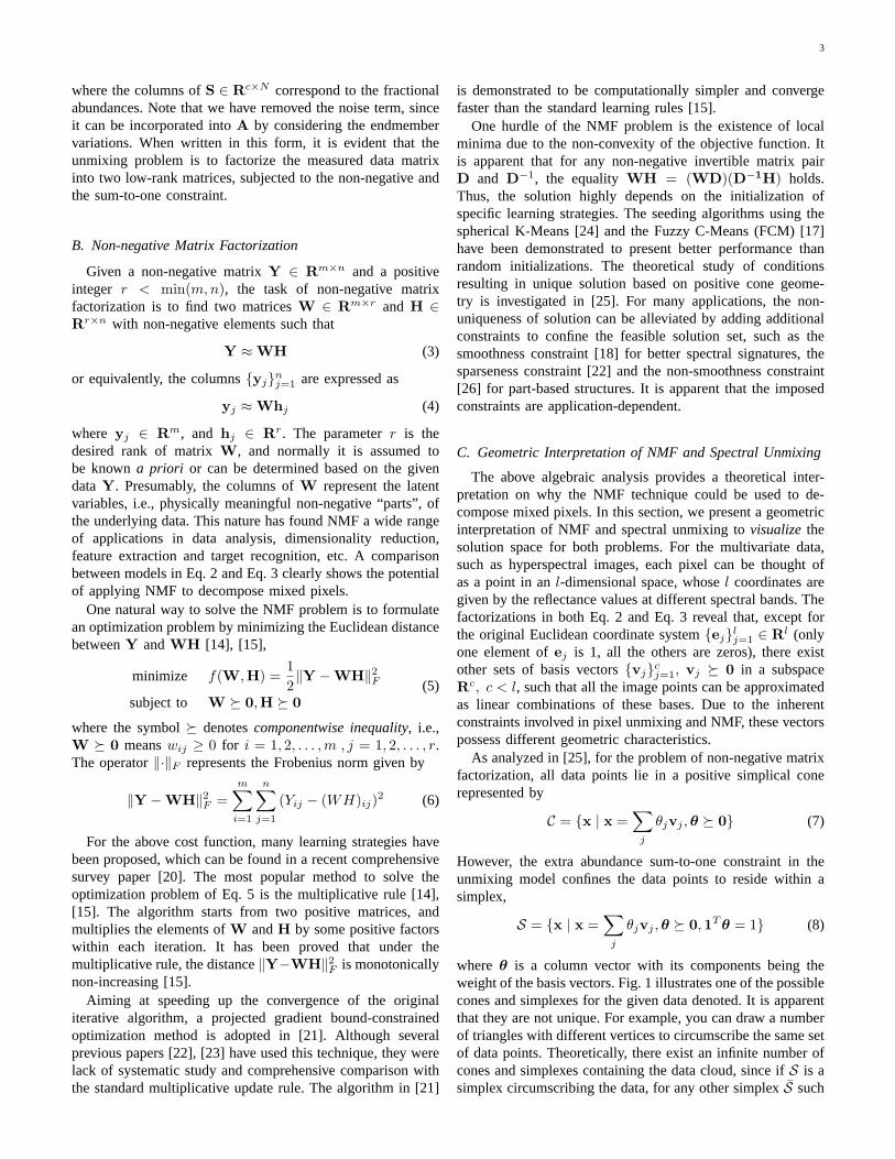
where θ is a column vector with its components being theweight of the basis vectors. Fig. 1 illustrates one of the possiblecones and simplexes for the given data denoted. It is apparentthat they are not unique. For example, you can draw a numberof triangles with different vertices to circumscribe the same setof data points. Theoretically, there exist an infinite number ofcones and simplexes containing the data cloud, since ifS is asimplex circumscribing the data, for any other simplexS such

4

E1

E2

E3

Cone C

Simplex S

Fig. 1. Geometric illustration of possible cones and simplexes that circum-scribe the given data denoted by the dots. The circlesE1 ∼ E3 can beconsidered as possible endmembers.

thatS ⊂ S, S will also contain the data. Then, one immediateand critical question would be what is the criterion for the bestsimplex solution or what properties the best simplex shouldpossess.

In the convex geometry-based endmember extraction al-gorithms, the best simplex is either defined as the one thatcircumscribes the data cloud and at the same time has theminimum volume [8], or defined as the one that inscribes thedata cloud with the maximum volume [10]. It is apparent thatunder the pure pixel assumption [9]–[11], the best simplexis uniquely determined by the pure pixels, which are thevertices of the simplex. The goal of endmember detectionis thus to identify the extreme-valued pixels from the givenimage. However, if all the image pixels are highly mixed, theidentified extreme points would not be the true endmembers,even though they are on the boundary of the data cloud andclose to the real ones. In order to find the true endmemberlocations from the highly mixed data, we have to extendthe searching space outside the given data cloud. In themeanwhile, we should keep the simplex that circumscribesthe data as compact as possible. These observations triggerthe development of the proposed algorithm by incorporatingthe minimum volume constraint into the NMF technique.

III. NMF WITH M INIMUM VOLUME CONSTRAINT

In this section, we describe the proposed minimum volumeconstrained NMF algorithm. To keep the symbols consistentduring the algorithm description, we will use the model inEq. 2 in the rest of the paper.

A. Problem Formulation

Combining the goal of minimum approximation error withthe volume constraint, we arrive at the following constrainedoptimization problem

minimize f(A,S) =12‖X−AS‖2F + λJ(A)

subject to A º 0, S º 0, 1Tc S = 1T

N

(9)

where 1c (1N ) is a c (N )-dimensional column vector ofall 1’s, and J(A) is the penalty function, calculating thesimplex volume determined by the estimated endmembers.The regularization parameterλ ∈ R is used to control thetradeoff between the accurate reconstruction and the volume

constraint. The first term serves as the external force to drivethe search to move outward, so that the generated simplexcontains all data points with relatively small errors. The secondterm serves as the internal force, which constrains the simplexvolume to be small. A solution is found when these twoforces balance each other. One of the expected advantages ofthe volume constrained NMF would be the resistance to thepresence of noise. The noise normally results in a bigger datacloud, which thereby leads to a simplex with larger volumethan the clean data, and the simplex vertices deviate from thetrue endmember locations. By adding the volume constraint,the simplex can be made not to include every data point,particularly, the noisy pixels on the boundary. Therefore, thealgorithm would be more robust to the noise effect than theunconstrained NMF approaches.

1) Volume Determination:In order to calculate the volumedetermined by a set of points, we hereby resort to the connec-tion between the volume and the determinant [27]. Supposewe havec affinely independent pointsa1, . . . ,ac ∈ Rc−1,which means that thec− 1 vectorsa2 − a1, . . . ,ac − a1 arelinearly independent. The volume determined by these pointsis calculated by

V =1

(c− 1)!

∣∣ det([a2 − a1 . . . ac − a1]

)∣∣ (10)

or equivalently,

V =1

(c− 1)!

∣∣ det([ 1 · · · 1

a1 · · · ac

])∣∣ (11)

Problem occurs when thesec points are in anl-space, i.e.,a1, . . . , ac ∈ Rl (c ≤ l), as the determinant is not defined fora non-square matrix. In this case, we make an approximationby calculating the volume formed by a new set of pointsa1, . . . , ac ∈ Rc−1, which is the low dimensional transformof the original data; that is, we adopt PCA to reduce thedimensionality of pointsa1, . . . ,ac from l to c−1 by keepingonly thec− 1 most significant principal components.

It is true that such volume determination can rarely returnthe actual volume formed by the endmembers. But recall thatthe real goal of this volume term is to constrain the simplexsize as compact as possible, provided that the vertices canapproximate the given data set at a certain error tolerance. Inthis sense, the computed volume is not necessarily the actualvalue, as long as it approximates the real one and performs asan internal force. The effectiveness of this constraint will bevalidated by a set of experiments reported in Section IV.

2) Cost Function:For the problem of Eq. 9, the simplexvolume is determined by thec endmembers, each of which isan l-dimensional vector (i.e., the columns ofA). Then,J(A)is formulated as

J(A) =1

2(c− 1)!det2(

[1T

c

A

]) (12)

where the matrixA = (a1, a2, . . . , ac) ∈ R(c−1)×c is a lowdimensional transform ofA given by

A = UT (A− µ1Tc ) (13)

5

The matrixU ∈ Rl×(c−1) is formed by thec−1 most signif-icant principal components (PCs) of dataX through principalcomponent analysis. The column vectorµ is the data mean.Note that both the PCs and the mean vector are calculatedfrom X instead ofA. One reason we formulate it in thisway is that the PCs of the given data points reflect importantshape information of the true simplex, thus the projection ontothis subspace reveals the similarity between the estimated andthe true simplex. In addition, from a computational efficiencypoint of view, the PCs ofX can be obtained through one timecalculation, while the PCs of the source matrixA need to berecalculated constantly asA changes.

To formulate the penalty term as a function ofA, we makethe following transformation. Let

Z =[

1Tc

A

]=

[1T

c

0

]+

[0T

c−1

I

]A (14)

where0 is a (c− 1)× c zero matrix,I is a (c− 1)× (c− 1)identity matrix, and0c−1 a (c− 1)-dimensional zero columnvector. The corresponding matrices are denoted by

C =[

1Tc

0

], B =

[0T

c−1

I

](15)

We then have

Z = C + BUT (A− µ1Tc ) (16)

Substituting the above equation into Eq. 12, and then Eq. 9,we finalize the objective function of the proposed MVC-NMFas

f(A,S) =12‖X−AS‖2F +

τ

2det2(C+BUT (A−µ1T

c )) (17)

with τ = λ(c−1)! , and the matricesC,B,U, and the vectorµ

are constants for the given dataX.

B. Optimization Algorithm Description

1) Initialization: To solve the formulated optimizationproblem, the first essential step is to determine the num-ber of endmembers involved in the mixture data, whichis always a challenge because it is closely related to theunknown noise. In the current research, we resort to thevirtual dimensionality (VD) method [28]. The algorithm aimsat finding the minimum number of spectrally distinct signalsources, which characterize the hyperspectral data from thetarget detection and classification point of view. Based onthe Neyman-Pearson detection theory, a hypothesis test isapplied to pairs of eigenvalues of the sample covariance matrixand the sample correlation matrix. The key is that when nosignal is present in a particular component, the correspondingcorrelation eigenvalue and covariance eigenvalue should beequal; otherwise, the covariance eigenvalue is less than the cor-responding correlation eigenvalue contributed by the correlatedsignals. To remove the second-order statistical correlation, anoise whitening process is incorporated as a preprocessingstep. Although the VD method is effective, it is not guaranteedthat the estimation is100% accurate. Therefore, the sensitivityanalysis of the proposed method to the estimated number of

endmembers is a very important issue. We will perform thisanalysis in Section IV.

The next question is how to initialize matricesA andS. As mentioned earlier, the unconstrained NMF algorithmsare sensitive to initializations due to the existence of localoptima. The algorithm performance highly depends on thedistance between the initial point and the global optimum.In this paper, we will show that by incorporating the proposedvolume constraint, this problem is successfully mitigated. Werandomly choosec points from the given data and arrangethem as the columns of the initialA. The value ofS can alsobe randomly initialized. In the experiments described in thispaper, a zero matrixS is used to start the learning.

2) Learning Rules:Minimizing the objective function inEq. 17 with respect to bothA and S is a combinatorialoptimization problem. We here resort to thealternating non-negative least squaresmethod [18], [21], [23]. This techniquetreats the original optimization problem as two sub-problemswith the following iterative update rule,

Ak+1 = arg minA

f(A,Sk) ≤ f(Ak,Sk)

Sk+1 = arg minS

f(Ak+1,S) ≤ f(Ak+1,Sk)(18)

that is, we alternatively update one matrix, holding the otherone fixed.

For each sub-problem, the projected gradient learning [18],[21], [22] is adopted to impose the non-negative constraint.The method of projected gradient follows the standard gradientlearning to update. When the new estimate does not satisfythe constraint, a projective function is used to project the pointback to the feasible set. For the non-negative constraint, we usea simple but effective functionmax(0, x) to set the negativecomponents to zero and keep the non-negative componentsunchanged. Then, the update rule is expressed as

Ak+1 = max(0, Ak − αk∇Af(Ak,Sk)

)

Sk+1 = max(0, Sk − βk∇Sf(Ak+1,Sk)

) (19)

where the parametersαk andβk are the small learning rates(stepsizes) selected based on the Armijo rule [29].

Let αo be the initial stepsize,σ ∈ (0, 12 ) be the tolerance,

and ρ ∈ (0, 1) the scaling factor that the stepsize is reducedin very iteration. Then, the Armijo rule chooses the stepsizeasαk = ρmkαo, wheremk is the first integer such that

f(Ak+1,Sk)− f(Ak,Sk) ≤ σρmkαo∇f(Ak,Sk)T (Ak+1 −Ak)

The stepsizeβk is selected based on the same procedure.Another important issue in the formulated problem is the

abundance sum-to-one constraint. This is an equality constraintand therefore can be dealt with using the Lagrange multipliersmethod with closed form solutions. In this paper, we adopt amuch simpler but effective method as in [30]. We augment thedata matrixX and the material signature matrixA by a rowof constant denoted by

X =[

Xδ1T

N

], A =

[A

δ1Tc

](20)

whereδ is a positive number to control the effect of the sum-to-one constraint. The learning of abundanceS described in

6

Eq. 19 takes these two augmented matrices as inputs. Asδincreases, the columns ofS are forced to approach the sum-to-one constraint. In order to balance between the estimationaccuracy and the convergence rate, we select a relatively smallδ, typically 10 ∼ 20, which results in abundances with thesummation varying between 0.998 and 1.002.

To implement the gradient learning, the first order derivative∇Af(A,S) and∇Sf(A,S) need to be calculated. Since thepenalty function is independent ofS, the partial derivative∇Sf(A,S) is easy to find,

∇Sf(A,S) = AT (AS−X) (21)

However, more algebraic operations need to be performed tocalculate∇Af(A,S). Taking the partial derivative of Eq. 17with respect toA, we first get

∇Af(A,S) = (AS−X)ST + τ det(Z)∂ det(Z)

∂A(22)

where Z is defined in Eq. 16. It is known that the partialderivative of a scalar with respect to a matrix is still a matrix,

∂ det(Z)∂A

=

∂ det(Z)∂a11

∂ det(Z)∂a12

· · · ∂ det(Z)∂a1c

∂ det(Z)∂a21

∂ det(Z)∂a22

· · · ∂ det(Z)∂a2c

......

...∂ det(Z)

∂al1

∂ det(Z)∂al2

· · · ∂ det(Z)∂alc

(23)

Then, the problem is tailored to compute each element of∂ det(Z)

∂A , which is given by

∂ det(Z)∂aij

= det(Z)Tr

(Z−1 ∂Z

∂aij

)(24)

It is easy to derive that

∂Z∂aij

=∂BUT A

∂aij(25)

Let D = BUT and Z = Z−1, through algebraic manipula-tions, we arrive at

Tr

(Z−1 ∂Z

∂aij

)= zT

j di (26)

wherezTj is thejth row of Z, anddi is theith column ofD.

Combining Eqs. 23, 24, and 26 gives

∂ det(Z)∂A

= det(Z)(ZE)T = det(Z)UBT (Z−1)T (27)

Substitute the above equation into Eq. 22, we obtain thegradient

∇Af(A,S) = (AS−X)ST + τdet2(Z)UBT (Z−1)T (28)

3) Stopping Conditions:For the NMF learning, differentstopping criteria have been exploited. The most commonlyused are the maximum iteration number and the error toler-ance. Several algorithms [21], [23] choose to stop the learningprocess whenever the Euclidean norm of the gradient of theobjective function is less than a threshold. Some implemen-tations [22] use an infinite loop, which needs user interactionto interrupt when some specific requirements are satisfied. For

the proposed minimization problem, we expect the objectivefunction to monotonically decrease. However, in order to avoidbeing trapped in local minima, we also allow certain steps ofincrease of the objective value. When the number of successiveincreasing steps is over a predefined value, the learning isstopped. In addition, we include an iteration limit specified bythe prescribed maximum iteration number.

The proposed MVC-NMF approach is summarized in Al-gorithm 1.

Algorithm 1: Minimum volume constrained NMF

Data : Non-negative mixture dataX ∈ Rl×N with eachcolumn being an observation vector.

Result: Two non-negative matricesA ∈ Rl×c and S ∈Rc×N with sum-to-one constraint1T

c S = 1TN .

//InitializationSetS = 0, i.e., a zero matrix;Set iteration indexk = 0;Estimate the number of endmembersc;Initialize A by randomly selectingc data points fromXto form its columns;

//main loopwhile stop conditions are not metdo

Ak+1 = max(0, Ak − αk∇Af(Ak,Sk));AugmentAk+1 to getAk+1;Sk+1 = max(0, Sk − βk∇Sf(Ak+1,Sk));Increasek by 1.

end

IV. EVALUATION WITH SYNTHETIC IMAGES

In this section, we conduct a series of experiments todemonstrate the effectiveness of the proposed MVC-NMFusing synthetic images. Note that, apart from the extractedendmembers, MVC-NMF deduces the fractional abundance ateach pixel as a by-product. In the following, we will evaluateboth the estimated endmembers and the inferred abundances.We compare with three existing approaches, namely VCA[5], NMF with smoothness constraint (SCNMF) [18], and theprojected gradient NMF method (PGNMF) [21], among whichVCA is a deterministic method, and the other two are bothNMF-based statistical approaches.

Regarding VCA, since it only identifies endmembers, weuse a fully constrained least squares method, called FCLS [30],to find the abundances. The objective of FCLS is to find theabundance vector by minimizing the least squares error‖x−As‖2. The algorithm integrates the constraint1T s = 1 intothe objective function by augmenting both the matrixA with arow vector of all 1’s and the observationx with an element of1. In this way, the original problem is converted to the standardnon-negative constrained least squares, which is solved using astandard active set method [31]. In the following, the combinedprocess of VCA and FCLS is referred to as VCA-FCLS.

For the two NMF approaches SCNMF [21] and PGNMF[18], the sum-to-one constraint is incorporated by the sameaugmenting technique as in Eq. 20. In addition, the last two

7

steps of SCNMF, i.e., finding the best match from a signaturedatabase, and calculating the abundance matrix using a leastsquares method, are eliminated for fair comparison.

A. Performance Metrics

The most widely used metric to measure the shape similaritybetween the true endmember signaturea and its estimatea isthe spectral angle distance (SAD), which is a high dimensionalextension to the two-dimensional geometric angle expressed as

SAD = cos−1

(aT a‖a‖‖a‖

)(29)

Another metric uses an information theoretic measure,spectral information divergence (SID) [32]. The probabilitydistribution vector associated with each endmember signatureis given byp = a∑

j aj. This vector can be used to describe

the variability of the spectral signature. Letp denote theprobability distribution vector of the estimatea. Then, thesimilarity betweena and a can be measured by the relativeentropy

D(a|a) =∑

j

pj log(pj

pj) (30)

Since the relative entropy is not symmetric, the followingmeasure is used

SID = D(a|a) + D(a|a) (31)

Regarding the abundance estimation, we use similar metricsby substituting the endmember signature with the abundancevector of each individual pixel, which gives the following twometrics

AAD = cos−1

(sT s‖s‖‖s‖

)(32)

andAID = D(s|s) + D(s|s) (33)

wheres represents the true abundance vector of a single pixeland s the corresponding estimate. AAD and AID refer tothe abundance angle distance and the abundance informationdivergence, respectively.

B. Creation of Synthetic Images

The synthetic images of size64 × 64 are generated usinga set of spectral reflectances selected from the USGS digitalspectral library [33]. The selection of endmember signatures isarbitrary as long as they are linearly independent. The spectraldata contain 224 spectral bands covering wavelengths from0.38µm to2.5µm with a spectral resolution of 10nm. To createlinear mixtures, we divide the entire image into units of8 ×8 small blocks. The pixels within each block are pure andhave the same type of ground cover, randomly selected asone of the endmember classes. The resulting image is thendegraded by a spatial low pass filter to simulate an image withmixed pixels. With this mixing method, we intend to simulatea hyperspectral scene with endmembers arranged in discretepatches so that a linear mixture model would be appropriate.The low pass filter we used is a simplek× k averaging filter.

Apparently, the value ofk controls the degree of mixing. Inthis paper, we use a9×9 filter to generate highly mixed data.To further remove pure pixels, we replace all the pixels whoseabundance is larger than80% with a mixture made up of allendmembers of equal abundances; that is, each endmemberhas an abundance of1/c in the mixture.

To simulate possible errors and sensor noise, we add zeromean Gaussian noise to the mixture data. Assuming the noiseis both spatially and spectrally uncorrelated, then the noisecovariance matrix is a diagonal matrixσ2I with I being anidentity matrix. Define the SNR asSNR = 10 log10

E[xT x]E[nT n]

,then the noise variance is easy to determine for a particularvalue of SNR, i.e.,σ2 = E[xT x]/(10SNR/10l).

C. Algorithm Evaluation

The proposed MVC-NMF algorithm is evaluated throughsix experiments. The first experiment aims to conduct an over-all comparison of different methods, including an illustrationof the approximation error and the effect of the introducedvolume constraint. In the second experiment, we study theperformance dependence of the NMF-based approaches ondifferent methods of initializations. The third experiment isdesigned to investigate the algorithm robustness to noisecorruptions. In the fourth experiment, we perform sensitivityanalysis of the proposed method to the accurate knowledgeof the number of endmembers. We then vary the numberof endmembers to create mixtures in the fifth experiment,aiming at investigating the algorithm generalizations to datasets with relatively large number of endmembers. In the lastexperiment, we study the algorithm performance when thegiven data contain pure endmember representations. In allthe experiments that follow, the quantitative measures areobtained by averaging 20 random tests. Four endmembers areused to create the synthetic mixtures for rapid computationin all experiments, except when we investigate the algorithmsensitivity to the estimated number of endmembers, and thegeneralization analysis to data sets with comparatively largenumbers of endmembers. All the NMF-based methods areinitialized randomly, except when we study the performancedependence on endmember initializations.

1) Overall comparison of different methods:In this exper-iment, we add 20dB white Gaussian noise to the syntheticmixtures and perform decomposition using different methods.The stopping criteria of PGNMF and MVC-NMF are thesame; that is, the algorithms are terminated when the iterationnumber of successive increase of the objective value is greaterthan 5, or the maximum iteration number, 150, is reached.The experimental results show that these two learning pro-cesses rarely use the maximum allowable number of iterations.Considering the low convergence of SCNMF, we allow themaximum number of iteration to be 300. In all the tests,the SCNMF learning ends up with very large approximationerrors at the 300th iteration, when the learning reaches itsstable state. The regularization parameter of MVC-NMF isselected asτ = 0.01. The parameters in all the other methodsimplemented in this paper follow their original work.

Fig. 2 demonstrates the experimental results, in which weshow both the mean (bar) and the standard deviation (error

8

bar). The SID value generated by MVC-NMF (Fig 2(d)) istoo small to tell, we thus label the result (mean/standarddeviation) aside its bar plot. As can be seen, MVC-NMFproduces the smallest means and standard deviations in termsof all measurement metrics used, indicating that this approachgenerates the most accurate and stable estimates. In addition,VCA-FCLS outperforms SCNMF and PGNMF. In terms ofabundance estimation (measured by AAD and AID), SCNMFproduces the largest means although with relatively smallerdeviations than PGNMF. Regarding the endmember extraction(measured by SAD and SID), it can be seen that the twomeasures present inconsistent comparisons between SCNMFand PGNMF. Overall, SCNMF yields smaller deviations thanPGNMF because of the use of the smoothness constraint,which tends to stabilize the endmember solutions.

VCA−FCLS SCNMF PGNMF MVC−NMF0

5

10

15

20

25

30

35

40

Different methods

AA

D m

easu

re

(a)VCA−FCLS SCNMF PGNMF MVC−NMF

0

1

2

3

4

5

6

Different methods

AID

mea

sure

(b)

VCA−FCLS SCNMF PGNMF MVC−NMF0

2

4

6

8

10

12

14

16

Different methods

SA

D m

easu

re

(c)

VCA−FCLS SCNMF PGNMF MVC−NMF0

0.05

0.1

0.15

0.2

0.25

0.3

0.35

0.4

0.45

0.5

Different methods

SID

mea

sure

0.003 / 0.001

(d)

Fig. 2. Performance comparison in terms of different metrics (SNR=20dB)(a) AAD (b) AID (c) SAD (d) SID.

We next fix the iteration number to 150 for the NMF-based methods and study the effect of the constrained volumeas well as the approximation error generated. In Fig. 3(a),the two constant profiles correspond to the volume derivedby VCA and that calculated using the real endmember set,respectively. As discussed before, VCA is deterministic andthe endmembers are chosen as the extreme points of thegiven data set. Therefore, the volume determined by the VCAestimates is smaller than that of the true endmembers. Theother three curves correspond to the results of the NMF-basedalgorithms. It can be seen that during the first few iterations,both the PGNMF and the MVC-NMF learning expand thesimplex rapidly. After that, the introduced volume constraintin MVC-NMF effectively confines the simplex volume tobe close to the true value. However, the PGNMF learningkeeps increasing the simplex size, which is much larger thanthe actual volume. And, the volume determined by SCNMFgrows very slowly as the learning goes. The approximationerror 1

2‖X−AS‖2F is plotted in Fig. 3(b), where we onlycompare the VCA-FCLS, the PGNMF, and the MVC-NMFlearning, as the SCNMF learning error is comparatively muchlarger even after convergence (more than 5 times that of theVCA-FCLS result). Again, the constant profile illustrates the

approximation error of VCA-FCLS. Note that during the first60 iterations, PGNMF yields smaller approximation errorsthan MVC-NMF and quickly converges to the stable state.After that, MVC-NMF continues to reduce the approximationerror and converges to a state with smaller error than PGNMF.This reveals that the PGNMF learning could be trapped in alocal minimum.

0 50 100 1500

5

10

15

20

25

30

35

Iteration

Vol

ume

TRUEVCASCNMFPGNMFMVC−NMF

(a)

0 50 100 1500

50

100

150

200

250

300

Iteration

Err

or

VCA−FCLSPGNMFMVC−NMF

(b)

Fig. 3. Comparison of the extracted endmembers and the estimation accuracyin terms of (a) Simplex volume (b) Approximation error.

Based on the above comparisons, we observe that thegeneral smoothness constraint adopted in SCNMF does notperform as well as the proposed volume constraint. In addition,SCNMF demonstrates slow convergence rate and much largerapproximation error. Therefore, in the following experiments,we exclude SCNMF for further comparisons and focus onthe comparative analysis between the deterministic (VCA-FCLS) and the statistical (PGNMF and MVC-NMF) methods,and between the unconstrained (PGNMF) and the constrained(MVC-NMF) NMF approaches.

2) Dependence analysis on endmember initializations:The purpose of this experiment is to show how differentinitialization methods could affect the NMF learning process.We study two methods for the endmember initialization, i.e.,random initialization and the use of the endmembers identifiedby VCA. The experimental results are shown in Fig. 4,where we display the deterministic results of VCA-FCLS,and the measures of PGNMF and MVC-NMF with differentinitialization schemes. One immediate observation we madeis that no matter which initialization methods are used, theproposed MVC-NMF always generates the smallest means andstandard deviations. In addition, PGNMF outperforms VCA-FCLS when initialized with the endmembers estimated byVCA, which, however, is not the case when using randominitializations. Another important observation is that MVC-NMF is less sensitive to the selection of the initial pointscompared to PGNMF. This observation leads to the conclusionthat the introduced volume constraint effectively confines thesolution space and converts the original ill-posed problem toa well-posed one.

3) Robustness analysis to noise corruptions:In this ex-periment, a comparative analysis on the issue of algorithmsensitivity to noise is studied by simulating synthetic data withdifferent noise levels. The SNR is varied to be 15dB, 25dB,45dB, and infinity (no noise is added). From the previousresults, we see that the angle distance and the informationdivergence metrics give similar comparison trend. It has alsobeen shown that the information divergence measure is more

9

VCA−FCLS PGNMF MVC−NMF0

5

10

15

20

25

Different methods

AA

D m

easu

re

Random init.VCA init.

(a)VCA−FCLS PGNMF MVC−NMF

0

0.5

1

1.5

2

2.5

3

Different methods

AID

mea

sure

Random init.VCA init.

(b)

VCA−FCLS PGNMF MVC−NMF0

2

4

6

8

10

12

Different methods

SA

D m

easu

re

Random init.VCA init.

(c)VCA−FCLS PGNMF MVC−NMF

0

0.05

0.1

0.15

0.2

0.25

Different methods

SID

mea

sure

Random init.VCA init.

0.004 / 0.002,0.003 / 0.003

(d)

Fig. 4. Performance comparison when PGNMF and MVC-NMF take randomand VCA initializations (SNR=10dB) (a) AAD (b) AID (c) SAD (d) SID.

effective in characterizing the spectral features [34]. Thus, inthe following experiments, we omit the AAD and SAD results.Fig. 5 compares the performance of different methods at var-ious noise levels. We observe, again, that the proposed MVC-NMF outperforms the others for all SNR cases. As the SNRincreases, both VCA-FCLS and MVC-NMF show improvedperformance. However, it is not the case for PGNMF, whichkeeps generating bad estimates no matter how clean the dataare. The reason is related to the ill-posedness of PGNMF,which is the dominating factor that affects its performance.

15 25 45 Inf0

0.5

1

1.5

2

2.5

3

3.5

4

4.5

5

SNR (dB)

AID

mea

sure

VCA−FCLSPGNMFMVC−NMF

(a)

15 25 45 Inf0

0.05

0.1

0.15

0.2

0.25

0.3

0.35

SNR (dB)

SID

mea

sure

VCA−FCLSPGNMFMVC−NMF

(b)

Fig. 5. Performance comparison at different noise levels in terms of (a) AID(b) SID.

4) Sensitivity analysis to the estimated number of endmem-bers: For a given data set, the number of endmembers cannotbe estimated with100% accuracy, especially when some of theendmembers are less prevalent and only present in a small setof pixels. Therefore, it is of importance to analyze the algo-rithm sensitivity to the estimated number of endmembers. Forthis purpose, we create a synthetic image with 6 endmembersand unmix the generated mixture using different numbers ofendmembers, varied from 3 to 9. Denote the actual numberof endmembers byc (c = 6) and the estimated value byc(c = 3, 4, . . . , 9), we compare the extracted endmembers withthe corresponding closest real endmembers whenc < c. Forthe situation ofc > c, we choose thec estimates which mostlyresemble the real endmembers and calculate the differences

in between. The abundances of the selected endmembers arethen used to compute AID. Fig. 6 illustrates the unmixingperformance with differentc values. The abundance estima-tion results shown in Fig. 6(a) demonstrate that the bestperformance of different methods occur whenc = c. As cdeviates fromc, the performances of VCA-FCLS and PGNMFdecrease accordingly. For the proposed MVC-NMF, the sametrend can be observed whenc < c. However, whenc > c,MVC-NMF produces steady estimates regardless of the valueof c. From the endmember extraction point of view, VCA-FCLS renders comparably stable performance as illustrated inFig. 6(b). This outcome is inherently related to the essence ofthe VCA scheme, which finds the extreme-valued pixels basedon geometrical projections. Thus, the identified extreme pointssolely depend on the data distribution. On the other hand, theproposed MVC-NMF aims at finding a convex hull to enclosethe data set. The shape of the convex hull is not only dependenton the data distribution, but also affected by the estimatednumber of endmembers, which determines the number ofextreme points of the convex hull. This dependence is muchobvious whenc < c as illustrated by the worse performanceof the NMF estimations in Fig. 6(b). Whenc > c, the NMF-based methods yield better results compared with the caseswhen c < c. This phenomenon can be explained by inspectingthe endmember profiles. We have observed that among theextractedc endmembers,c− c estimates are very similar withthe others, indicating that the true dimension of the estimatedendmembers is equal toc. Therefore, the increasedc doesnot change the shape of the reconstructed convex hull verymuch, which also explains why MVC-NMF generates steadyabundance estimations whenc > c. This example shows thatthe success of MVC-NMF relies on the correct knowledge ofc.

3 4 5 6 7 8 90

1

2

3

4

5

6

7

8

9

10

Estimated number of endmembers

AID

mea

sure

VCA−FCLSPGNMFMVC−NMF

(a)

3 4 5 6 7 8 90

0.2

0.4

0.6

0.8

1

1.2

Estimated number of endmembers

SID

mea

sure

VCA−FCLSPGNMFMVC−NMF

0.003 / 0.002

(b)

Fig. 6. Illustration of sensitivity to the estimated number of endmembers.The actual number of endmembers is 6 (SNR=20dB). (a) AID (b) SID.

5) Generalization to larger numbers of endmembers:In thisexperiment, the algorithm is evaluated with images containingdifferent numbers of endmembers. We vary the number ofendmembers fromc = 3 to c = 10 and create a set of syn-thetic images. Fig. 7 illustrates the unmixing performance ofdifferent methods, where the SID measures are the logarithmictransforms given byy = log(1+x), with x denoting the actualSID value andy the transformed result. This transformation isused to suppress the big difference between the PGNMF andthe MVC-NMF estimates for better visual comparisons. Ascan be seen that MVC-NMF provides the best performance forimages with different numbers of endmembers, while PGNMF

10

displays the worst results. Examining the results of VCA-FCLS and MVC-NMF, the AID measures increase slightlyas the number of endmembers present in the mixture dataincreases, while the SID measures is less dependent of thisparameter by illustrating very similar results when differentnumbers of endmembers are used.

3 4 5 6 7 8 9 100

1

2

3

4

5

6

7

Number of endmembers

AID

mea

sure

VCA−FCLSPGNMFMVC−NMF

(a)

3 4 5 6 7 8 9 100

0.05

0.1

0.15

0.2

0.25

0.3

0.35

Number of endmembers

SID

mea

sure

VCA−FCLSPGNMFMVC−NMF

(b)

Fig. 7. Performance comparison when applied to images created by mixingdifferent numbers of endmembers (SNR=20dB) (a) AID (b) SID (The SIDplot displays the logarithmic transforms of actual values for better visualcomparisons).

6) Generalization to images containing pure pixel repre-sentations: Although the proposed method is motivated byunmixing highly mixed images, it is important to study itsgeneralization to the mixture data containing pure pixels. Forthis purpose, we take a7×7 low pass filter to create syntheticmixtures so that the created images contain pure pixels. Theexperimental results are illustrated in Fig. 8. Similarly, the SIDresults are displayed in terms of the logarithmic transforms.Note that MVC-NMF generates the smallest mean and slightlyworse (in terms of AID) or the same (in terms of SID) standarddeviation as VCA-FCLS. This result leads to an importantconclusion that MVC-NMF is not specific for unmixing highlymixed data. It can also produce reliable unmixing results whenapplied to hyperspectral images containing pure pixels, whichfurther broadens the application domain of the proposed MVC-NMF method.

VCA−FCLS PGNMF MVC−NMF0

0.5

1

1.5

2

2.5

3

3.5

4

Different methods

AID

mea

sure

(a)VCA−FCLS PGNMF MVC−NMF

0

0.05

0.1

0.15

0.2

0.25

0.3

Different methods

SID

mea

sure

(b)

Fig. 8. Performance comparison when the image contains pure pixels(SNR=20dB) (a) AID (b) SID (The SID results are the logarithmic transformsof actual measures).

V. EVALUATION WITH REAL IMAGE SCENE

In this section, we apply the MVC-NMF algorithm to realhyperspectral data captured by the Airborne Visible/InfraredImaging Spectrometer (AVIRIS) over Cuprite, Nevada. TheAVIRIS sensor is a 224-channel imaging spectrometer withapproximately 10nm spectral resolution covering wavelengthsranging from 0.4µm to 2.5µm. The spatial resolution is 20m.We have chosen this test site for several reasons. First, this

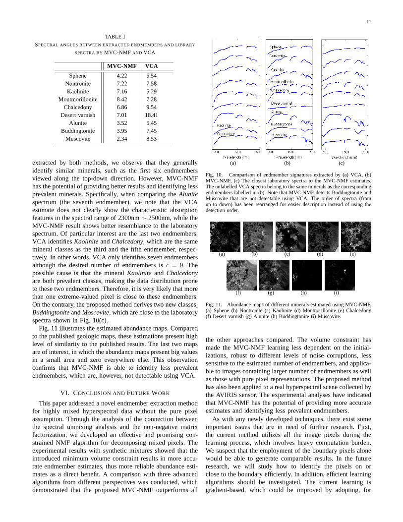
site has been extensively used for remote sensing experimentssince the 1980s, and many research work have been publishedwith high-accuracy ground truth available [11], [35], [36]; sec-ondly, the Cuprite area is a relatively undisturbed hydrothermalsystem with many well exposed minerals. More importantly,some of the minerals are prevalent, while others are highlymixed in a small set of pixels. The selected subscene is shownin Fig. 9, which consists of 200 lines and 200 pixels per line.To improve the unmixing performance, we have removed thelow SNR bands as well as the water vapor absorption bands(including bands 1-2, 104-113, 148-167 and 221-224) fromthe original 224-band data cube. So, a total of 188 bands areused in the experiment.

Fig. 9. Band 30 of the real hyperspectral scene

In order to evaluate the performance of MVC-NMF appliedto real hyperspectral scenes, we perform two comparisons:the comparison between the extracted endmembers and thelaboratory spectra; and the comparison between the derivedabundance maps and the published results. For each detectedendmember, we find the closest match from the spectral librarybased on the spectral correlation defined as

corr =(a− β)T (al − βl)

‖a− β‖‖al − βl‖(34)

wherea andal correspond to the estimated spectrum and thelibrary spectrum. Their mean values, denoted byβ andβl, aresubtracted from the original spectra to give accurate correlationcoefficients. The library spectrum with the highest correlationis chosen as the best match. However, this correlation mightsuffer from mismatch. To mitigate this drawback, we furthervisually compare the derived abundance maps to the detailedmineral maps provided in [36]. If an obvious mismatch occursduring the finding of the closest signature from the spectrallibrary, we rely on the classification based on the abundancedistribution.

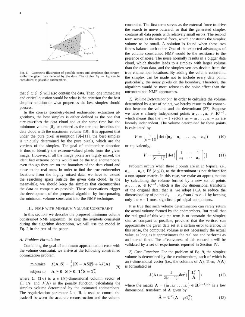
The estimated number of endmembers using the VD method[28] is equal toc = 9. We use the VCA estimates as thestarting points for the MVC-NMF learning. The extractedendmembers by VCA and MVC-NMF are shown in Fig. 10(a)and (b), respectively. Fig. 10(c) displays the closest labo-ratory spectra to the MVC-NMF results. We have labelledthe endmember classes in Fig. 10(b), and the correspondingunlabelled VCA spectra belong to the same mineral classes.The comparisons of MVC-NMF and VCA in terms of spectralangles between extracted endmembers and laboratory signa-tures are summarized in Table I. Quantitatively, MVC-NMFgenerates smaller spectral angles than VCA in most cases,which means its estimates better resemble the laboratory data.

By side-by-side visual comparison of the endmembers

11

TABLE I

SPECTRAL ANGLES BETWEEN EXTRACTED ENDMEMBERS AND LIBRARY

SPECTRA BYMVC-NMF AND VCA

MVC-NMF VCA

Sphene 4.22 5.54Nontronite 7.22 7.58Kaolinite 7.16 5.29

Montmorillonite 8.42 7.28Chalcedony 6.86 9.54

Desert varnish 7.01 18.41Alunite 3.52 5.45

Buddingtonite 3.95 7.45Muscovite 2.34 8.53

extracted by both methods, we observe that they generallyidentify similar minerals, such as the first six endmembersviewed along the top-down direction. However, MVC-NMFhas the potential of providing better results and identifying lessprevalent minerals. Specifically, when comparing theAlunitespectrum (the seventh endmember), we note that the VCAestimate does not clearly show the characteristic absorptionfeatures in the spectral range of 2300nm∼ 2500nm, while theMVC-NMF result shows better resemblance to the laboratoryspectrum. Of particular interest are the last two endmembers.VCA identifiesKaolinite andChalcedony, which are the samemineral classes as the third and the fifth endmember, respec-tively. In other words, VCA only identifies seven endmembersalthough the desired number of endmembers isc = 9. Thepossible cause is that the mineralKaolinite and Chalcedonyare both prevalent classes, making the data distribution proneto these two endmembers. Therefore, it is very likely that morethan one extreme-valued pixel is close to these endmembers.On the contrary, the proposed method derives two new classes,BuddingtoniteandMoscovite, which are close to the laboratoryspectra shown in Fig. 10(c).

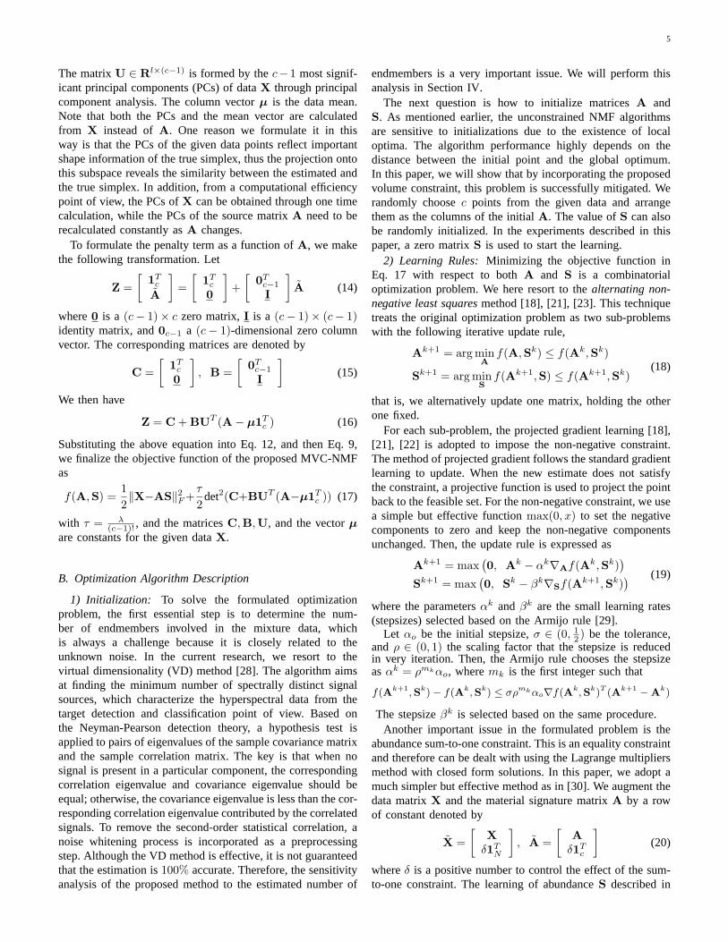
Fig. 11 illustrates the estimated abundance maps. Comparedto the published geologic maps, these estimations present highlevel of similarity to the published results. The last two mapsare of interest, in which the abundance maps present big valuesin a small area and zero everywhere else. This observationconfirms that MVC-NMF is able to identify less prevalentendmembers, which are, however, not detectable using VCA.

VI. CONCLUSION AND FUTURE WORK

This paper addressed a novel endmember extraction methodfor highly mixed hyperspectral data without the pure pixelassumption. Through the analysis of the connection betweenthe spectral unmixing analysis and the non-negative matrixfactorization, we developed an effective and promising con-strained NMF algorithm for decomposing mixed pixels. Theexperimental results with synthetic mixtures showed that theintroduced minimum volume constraint results in more accu-rate endmember estimates, thus more reliable abundance esti-mates as a direct benefit. A comparison with three advancedalgorithms from different perspectives was conducted, whichdemonstrated that the proposed MVC-NMF outperforms all

(a) (b) (c)

Fig. 10. Comparison of endmember signatures extracted by (a) VCA, (b)MVC-NMF, (c) The closest laboratory spectra to the MVC-NMF estimates.The unlabelled VCA spectra belong to the same minerals as the correspondingendmembers labelled in (b). Note that MVC-NMF detects Buddingtonite andMuscovite that are not detectable using VCA. The order of spectra (fromup to down) has been rearranged for easier description instead of using thedetection order.

(a) (b) (c) (d) (e)

(f) (g) (h) (i)

Fig. 11. Abundance maps of different minerals estimated using MVC-NMF.(a) Sphene (b) Nontronite (c) Kaolinite (d) Montnorillonite (e) Chalcedony(f) Desert varnish (g) Alunite (h) Buddingtonite (i) Muscovite.

the other approaches compared. The volume constraint hasmade the MVC-NMF learning less dependent on the initial-izations, robust to different levels of noise corruptions, lesssensitive to the estimated number of endmembers, and applica-ble to images containing larger number of endmembers as wellas those with pure pixel representations. The proposed methodhas also been applied to a real hyperspectral scene collected bythe AVIRIS sensor. The experimental analyses have indicatedthat MVC-NMF has the potential of providing more accurateestimates and identifying less prevalent endmembers.

As with any newly developed techniques, there exist someimportant issues that are in need of further research. First,the current method utilizes all the image pixels during thelearning process, which involves heavy computation burden.We suspect that the employment of the boundary pixels alonewould be able to generate comparable results. In the futureresearch, we will study how to identify the pixels on orclose to the boundary efficiently. In addition, efficient learningalgorithms should be investigated. The current learning isgradient-based, which could be improved by adopting, for

12

example, the second-order methods.

REFERENCES

[1] G. M. Foody, Remote Sensing Image Analysis: Including the SpatialDomain. Kluwer Academic Publishers, 2004, ch. 3, pp. 37–49.

[2] N. Keshava, “A survey of spectral unmixing algorithms,”Lincoln Lab-oratory Journal, vol. 14, no. 1, pp. 55–78, 2003.

[3] M. O. Smith, P. E. Johnson, and J. B. Adams, “Quantitative determi-nation of mineral types and abundances from reflectance spectral usingprincipal components analysis,”J. Geophys. Res., no. 90, pp. C797–C804, 1985.

[4] J. Bayliss, J. A. Gualtieri, and R. Cromp, “Analyzing hyperspectral datawith independent component analysis,” inProc. of SPIE, vol. 3240,1997, pp. 133–143.

[5] J. M. P. Nascimento and J. M. B. Dias, “Does independent componentanalysis play a role in unmixing hyperspectral data,”IEEE Trans.Geosci. Remote Sensing, vol. 43, no. 1, pp. 175–184, Jan. 2004.

[6] G. Healey and D. Slater, “Models and methods for automated ma-terial identification in hyperspectral imagery acquired under unknownillumination and atmospheric conditions,”IEEE Trans. Geosci. RemoteSensing, vol. 37, no. 6, pp. 2706–2717, 1999.

[7] J. W. Boardman, “Automating spectral unmixing of aviris data usingconvex geometry concepts,” inSummaries of the fourth annual JPLairborne geoscience workshop, R. O. Green, Ed., 1994, pp. 11–14.

[8] M. D. Craig, “Minimum-volume transforms for remotely sensed data,”IEEE Trans. Geosci. Remote Sensing, vol. 32, no. 3, pp. 542–552, May1994.

[9] J. W. Boardman, F. A. Kruse, and R. O. Green, “Mapping targetsignatures via partial unmixing of aviris data,” inSummaries of FifthAnnual JPL Airborne Geoscience Workshop, R. O. Green, Ed., vol. 1,1995, pp. 23–26.

[10] M. E. Winter, “Fast autonomous spectral endmember determination inhyperspectral data,” inProc. of 13th international conference on appliedgeologic remote sensing, vol. 2, Vancouver, BC, Canada, 1999, pp. 337–344.

[11] J. M. P. Nascimento and J. M. B. Dias, “Vertex component analysis: afast algorithm to unmix hyperspectral data,”IEEE Trans. Geosci. RemoteSensing, vol. 43, no. 4, pp. 898–910, Apr. 2005.

[12] V. F. Haertel and Y. E. Shimabukuro, “Spectral linear mixing model inlow spatial resolution image data,”IEEE Trans. Geosci. Remote Sensing,vol. 43, no. 11, pp. 2555–2562, Nov. 2005.

[13] M. Berman, H. Kiiveri, R. Lagerstrom, A. Ernst, R. Dunne, and J. F.Huntington, “Ice: A statistical approach to identifying endmembers inhyperspectral images,”IEEE Trans. Geosci. Remote Sensing, vol. 42,no. 10, pp. 2085–2095, Oct. 2004.

[14] D. Lee and S. Seung, “Learning the parts of objects by non-negativematrix factorization,”Nature, vol. 401, pp. 788–791, 1999.

[15] ——, “Algorithms for non-negative matrix factorization,” inAdvancesin Neural Information Processing Systems, vol. 13. MIT Press, 2001,pp. 556–562.

[16] L. C. P. P. Sajda, S. Du, “Recovery of constituent spectra using non-negative matrix factorization,” inProceedings of SPIE, vol. 5207, 2003.

[17] C.-Y. Liou and K. O. Yang, “Unsupervised classification of remotesensing imagery with non-negative matrix factorization,” inICONIP,2005.

[18] V. P. Paura, J. Piper, and R. J. Plemmons, “Nonnegative matrix fac-torization for spectral data analysis,”To appear in Linear Algebra andApplications, 2006.

[19] J. J. Settle and N. A. Drake, “Linear mixing and the estimation of groundcover proportions,”Int. J. Remote sensing, vol. 14, no. 6, pp. 1159–1177,1993.

[20] M. W. Berry, M. Browne, A. N. Langville, V. P. Pauca, and R. J.Plemmons, “Algorithms and applications for approximate nonnegativematrix factorization,”Preprint submitted to Elsevier, 2006.

[21] C.-J. Lin, “Projected gradient methods for non-negative matrix factor-ization.” Department of Computer Science, National Taiwan University”Technical report, 2005.

[22] P. O. Hoyer, “Non-negative matrix factorization with sparseness con-straints,”Journal of Machine Learning Research, vol. 5, pp. 1457–1469,2004.

[23] M. Chu, F. Diele, R. Plemmons, and S. Ragni, “Optimality, computa-tion, and interpretations of nonnegative matrix factorizations,”AvailableOnline: http://www.wfu.edu/ plemmons, 2004.

[24] S. M. Wild, “Seeding non-negative matrix factorizations with thespherical k-means clustering,” M.S. Thesis, Department of AppliedMathematics, University of Colorado, Apr 2003.

[25] D. Donoho and V. Stodden, “When does non-negative matrix factor-ization give a correct decomposition into parts,” inAdvances in NeuralInformation Processing Systems 16, S. Thrun and B. Scholkopf, Eds.Cambridge, MA: MIT Press, 2004.

[26] A. Pascual-Montano, J. Carazo, K. Kochi, D. Lehmann, and R. D.Pascual-Marqui, “Nonsmooth nonnegative matrix factorization (nsnmf),”IEEE Transactions on Pattern Analysis and Machine Intelligence,vol. 28, no. 3, pp. 403–415, Mar 2006.

[27] G. Strang,Linear Algebra and its application, 3rd ed. MassachusettsInstitute of Technology, 1988.

[28] C.-I. Chang and Q. Du, “Estimation of number of spectrally distinctsignal sources in hyperspectral imagery,”IEEE Trans. Geosci. RemoteSensing, vol. 42, no. 3, pp. 608–619, Mar. 2004.

[29] M. P. Bertsekas,Constrained Optimization and Lagrange MultiplierMethods. Academic Press, 1982.

[30] D. C. Heinz and C.-I. Chang, “Fully constrained least squares linearspectral mixture analysis method for material quantification in hyper-spectral imagery,”IEEE Trans. Geosci. Remote Sensing, vol. 39, no. 3,pp. 529–545, Mar. 2001.

[31] R. Bro and S. D. Jong, “A fast non-negativity constrained least squaresalgorithm,” J. Chemom., vol. 11, pp. 393–401, 1997.

[32] C.-I. Chang and D. C. Heinz, “Constrained subpixel target detection forremotely sensed imagery,”IEEE Trans. Geosci. Remote Sensing, vol. 38,no. 3, pp. 1144–1159, May 2000.

[33] R. N. Clark, G. A. Swayze, A. Gallagher, T. V. King, and W. M. Calvin,“The u.s. geological survey digital spectral library: Version 1:0.2 to 3.0µm,” U.S. Geol. Surv.,” Open File Rep. 93-592, 1993.

[34] C. Kwan, B. Ayhan, G. Chen, J. Wang, B. Ji, and C.-I. Chang, “Anovel approach for spectral unmixing, classification, and concentrationestimation of chemical and biological agents,”IEEE Trans. Geosci.Remote Sensing, vol. 44, no. 2, pp. 409–419, Feb. 2006.

[35] G. Swayze, R. Clark, S. Sutley, and A. Gallagher, “Ground-truthingaviris mineral mapping at cuprite, nevada,” inSummaries 3rd Annu.JPL Airborne Geosciences Workshop, vol. 1, 1992, pp. 47–49.

[36] G. Swayze, “The hydrothermal and structural history of the cupritemining district, southwestern nevada: An integrated geological and geo-physical approach,” PhD Dissertation, University of Colorado, Boulder,1997.

Lidan Miao (S’04) received her BS. and MS.degrees in Electrical Engineering from Sichuan Uni-versity, China, in 2000 and 2003, respectively. Since2004, she has been pursuing her PhD degree in theDepartment of Electrical and Computer Engineering,University of Tennessee, Knoxville, TN.

Her current research interests include signal andimage processing, pattern recognition, and remotesensing. She is a student member of IEEE.

Hairong Qi (SM’05) received her Ph.D. degree inComputer Engineering from North Carolina StateUniversity in 1999, B.S. and M.S. degrees in Com-puter Science from Northern JiaoTong University,Beijing, P.R.China in 1992 and 1995 respectively.

She is now an Associate Professor in the De-partment of Electrical and Computer Engineering atthe University of Tennessee, Knoxville. Her currentresearch interests are advanced imaging and collab-orative processing in sensor networks, hyperspectralimage analysis, and bioinformatics. She has pub-

lished over 70 technical papers in archival journals and refereed conferenceproceedings, including a co-authored book in Machine Vision.

Dr. Qi is the recipient of the NSF CAREER award, Chancellor’s Award forProfessional Promise in Research and Creative Achievement. She serves onthe editorial board of Sensor Letters and is the Associate Editor for Computersin Biology and Medicine.