endgame strategies for planetary m...
TRANSCRIPT
ENDGAME STRATEGIES FOR PLANETARY MOON ORBITERS
by
RYAN WOOLLEY
B.S., PHYSICS-ASTRONOMY, BRIGHAM YOUNG UNIVERSITY, 2003
M.S., ASTRONAUTICAL ENGINEERING, UNIVERSITY OF SOUTHERN CALIFORNIA, 2005
A thesis submitted to the
Faculty of the Graduate School of the
University of Colorado in partial fulfillment
of the requirements for the degree of
Doctor of Philosophy
Department of Aerospace Engineering Sciences
2010
This thesis entitled:
Endgame Strategies for Planetary Moon Orbiters
written by Ryan Woolley
has been approved for the
Department of Aerospace Engineering Sciences
Daniel Scheeres
George Born
Steve Nerem
Rodney Anderson
Elizabeth Bradley
Date_______________
The final copy of this thesis has been examined by the signatories, and we find that
both the content and the form meet acceptable presentation standards of scholarly
work in the above-mentioned discipline.
iii
ABSTRACT
Woolley, Ryan Cliff (Ph.D. Aerospace Engineering Sciences)
Endgame Strategies for Planetary Moon Orbiters
Directed by Daniel Scheeres, Professor, Department of Aerospace Engineering
Sciences, University of Colorado at Boulder
Delivering an orbiter to a planetary moon such as Titan or Europa requires an
exorbitant amount of fuel if the trajectory is not carefully and cleverly planned. V-
infinity leveraging maneuvers are an effective means to reduce total Delta-V
requirements to achieve orbit about a planetary satellite. This work seeks to
characterize optimal trajectories making use of flybys, leveraging maneuvers, and
capture orbits in order to minimize fuel requirements. With the aid of customized
tools to construct, map, and analyze sequences of resonances and maneuvers, we
derive heuristics of global optima and formulate a theoretical minimum. The
theoretical minimum, which is found using an infinite series of flybys and leveraging
maneuvers, results in a Delta-V savings of over 70% when compared to a direct
insertion during flyby. We then generate numerical results, which show that the
optimal location for performing V-infinity reduction maneuvers is not necessarily at
apoapsis, due to targeting constraints. By plotting total Delta-V vs. time-of-flight for
tens of thousands of generated sequences, a Pareto front is created of the most
iv
efficient sequences for each given flight time. This Pareto front shows that while
infinite missions are not possible, it is feasible to reduce the total Delta-V by 50%
with only a modest increase in flight time. Increasing the mission duration further
does not result in significant reductions.
It is shown that periodic orbits exist in the restricted three-body problem
whose Jacobi constants correspond to a positive V-infinity in the two-body problem.
This indicates that these orbits are classically hyperbolic and yet are gravitationally
bound to the vicinity of the target body. This dissertation explores the limits and
usefulness of these hyperbolic periodic orbits and their application to the endgame
problem. Families of orbits are generated using a single shooting method and
integrated into the final phase of V-infinity leveraging sequences. Using a hyperbolic
periodic orbit to capture to the vicinity of a target moon following an optimized
sequence of leveraging maneuvers and flybys yields significant fuel savings (60-70%)
over direct trajectories.

DEDICATION
This dissertation is dedicated to my wife, Venessa, and to my beautiful young
children, Jeremy and Chloe. My quest for more education brought you into my life,
and for that I will be eternally grateful.
“…yea, and all things denote there is a God; yea, even the
earth, and all things that are upon the face of it, yea, and its
motion, yea, and also all the planets which move in their
regular form do witness that there is a Supreme Creator.”
Alma 30:44
vi
ACKNOWLEDGEMENTS
First and foremost, I need to thank my wife, Venessa, for loving me
unconditionally and supporting me more than I could have imagined was possible.
Your love and encouragement help me to believe that I can accomplish anything. You
believed in me and helped pick me up when I was discouraged. Your ability to
understand science and engineering constantly amazes me. The conversations we
have had about my research made my project better and allowed me to complete this
dissertation. Your expertise in technical editing has kept this dissertation readable and
intelligible. I cannot thank you enough for all of the help you have provided.
I am also indebted to Dr. Scheeres for his constant support in this research.
He helped me focus my efforts and steered me through the difficulties incumbent
upon projects of this magnitude. His ability to immediately delve right into the
deepest subject matter and recall governing principles and equations always astounds
me.
I began my time at the University of Colorado under the guidance of Dr.
George Born, whose reputation and accomplishments brought me to the university in
the first place. I am grateful for all the time he spent with me as my advisor over the
first two years of my study. Dr. Born was also instrumental in my acquiring a part
time research position at the Laboratory of Atmospheric and Space Physics (LASP),
which funded the majority of my studies here in Colorado. I also met many
vii
wonderful and brilliant people at LASP as well as learning many valuable skills that
will serve me well throughout my career.
I also wish to thank my fellow graduate students with whom I have had the
pleasure to associate. Jeff Parker, Brandon Jones, Rodney Anderson, and Kate Davis
served as excellent TA’s for interplanetary mission design and quickly became
mentors, teammates, and friends that made my experience here all the more
enjoyable.
viii
CONTENTS
1 Introduction........................................................................................................... 1
1.1 Motivation .................................................................................................... 2
1.2 Problem Characterization............................................................................. 4
1.3 Historical Roots............................................................................................ 8
1.3.1 A Brief History of Two-Body Problem .......................................... 9
1.3.2 A Brief History of the Three-Body Problem ................................ 10
1.3.3 Recent Related Work .................................................................... 12
1.4 Contributions of This Dissertation ............................................................. 14
1.5 Dissertation Organization........................................................................... 18
2 Models and Methods........................................................................................... 20
2.1 The Two-Body Problem............................................................................. 20
2.1.1 Orbital Parameters ........................................................................ 23
2.1.2 Orbital Transfers ........................................................................... 25
2.1.3 Lambert’s Problem........................................................................ 27
2.1.4 The Dynamics of a Gravity-Assist Flyby ..................................... 31
2.1.5 Patched Two-Body Trajectories ................................................... 36
2.2 The Three-Body Problem........................................................................... 38
2.2.1 Planar Circular Restricted Three-Body Problem .......................... 38
2.2.2 Equations of Motion and Normalization....................................... 40
ix
2.2.3 Jacobi Constant ............................................................................. 41
2.2.4 Hill’s Problem............................................................................... 41
2.2.5 The Jacobi Integral – PR3BP vs. Hill’s ........................................ 44
2.2.6 Propagating Orbits and the State Transition Matrix ..................... 45
2.2.7 Stability and the Monodromy Matrix ........................................... 47
2.2.8 The Single-Shooting Method........................................................ 48
2.2.9 The Inertial Frame and Tisserand’s Invariant ............................... 49
2.2.10 Normalization Parameters............................................................. 52
2.3 Relationships between the Two- and Three-Body Problems ..................... 53
3 V∞ Leveraging...................................................................................................... 55
3.1 Introduction ................................................................................................ 56
3.2 Models and Normalization ......................................................................... 61
3.3 The V∞ Sphere ............................................................................................ 63
3.3.1 Accessible Regions ....................................................................... 65
3.3.2 Shrinking the V∞ Sphere ............................................................... 67
3.4 Designing V∞ Leveraging Maneuvers ........................................................ 71
3.4.1 The Lambert Solution Technique ................................................. 72
3.4.2 V∞ Leveraging Efficiency ............................................................. 74
3.5 Theoretical Minimum ∆V........................................................................... 79
3.5.1 Practical Considerations................................................................ 83
3.6 Global Search Methodology....................................................................... 85
3.6.1 Simulations ................................................................................... 86
3.7 Results ........................................................................................................ 90
x
3.8 Conclusion.................................................................................................. 97
4 Hyperbolic Periodic Orbits ................................................................................ 99
4.1 Introduction ................................................................................................ 99
4.2 Families of planar periodic orbits with positive V∞’s............................... 101
4.2.1 Hyperbolic Periodic Orbits as Capture Mechanisms .................. 112
4.3 Conclusion................................................................................................ 116
5 Discussion .......................................................................................................... 118
5.1 Overview of Findings............................................................................... 118
5.1.1 Contributions to the Field ........................................................... 119
5.1.2 Areas of Future Research............................................................ 120
6 Bibliography...................................................................................................... 122
7 Appendix A: Nomenclature ............................................................................. 128
8 Appendix B: Coordinate Transformations.................................................... 131
9 Appendix C: Notes on Lambert’s Problem ................................................... 133
9.1 Lambert’s Theorem .................................................................................. 133
9.2 Multi-Revolution Solutions to Lambert’s Problem.................................. 135
10 Appendix D: Tables of V∞ Leveraging Sequences ........................................ 139
xi
LIST OF TABLES
Table 2.1. Normalization Parameters for a Few Moons. ........................................... 53
Table 3.1. Normalization Parameters for a Few Celestial Bodies ............................. 63
Table 3.2. Maneuver Sequence for an Example Tour. This tour has a resonance
sequence of 2:1, 3:1, 4:1, 5:1, 6:1. Maneuvers consist of ∆V’s (DV),
which are performed during fly-by (PFB) or as a leveraging
maneuver (VILM), and fly-bys (FB). Values for V∞ (initial and
final), resonance (initial and final), efficiency, ∆V, times, α, and δmax
are given for each maneuver.................................................................... 87
Table 3.3. The 10 Shortest TOF Sequences for Vc = 0.3. Parentheses represent
phasing orbits and ‘NT’ indicates a resonance that started out non-
tangentially (i.e. α > 0)............................................................................. 92
Table 3.4. The 10 Lowest Total ∆V Sequences for Vc = 0.3. Each resonance in
the sequence includes a leveraging maneuver. ........................................ 93
Table 4.1. Selected Hyperbolic Periodic Orbits at Titan (µ = 2.366e-4). Values
given are for the point of closest approach. rp is given in Titan radii
(negative values correspond to passage on the Saturn side of Titan)
xii
and the other parameters are normalized using the conventions of the
3BP. xr and ry& are in the rotating frame with respect to the
barycenter. P is the orbit period. xi,2 and 2,iy& are inertial with respect
to Titan. V∞ (3-body) is calculated using the approximation in
Equation 2.83 whereas V∞ (2-body) is calculated using Equation 4.1. . 108
Table 10.1. Top Sequences with Vc = 0.3 and no crossing of the δmax line (NX).... 140
Table 10.2. Top Sequences with Vc = 0.3 and phasing (PH). ................................... 142
Table 10.3. Top Sequences with Vc = 0.3 and non-tangential (NT) leveraging ....... 144
Table 10.4. Most efficient sequences for Vc = 0.2. .................................................. 146
Table 10.5. Fastest sequences for Vc = 0.2............................................................... 147
Table 10.6 Fastest sequences for Vc = 0.1................................................................ 148
xiii
LIST OF FIGURES
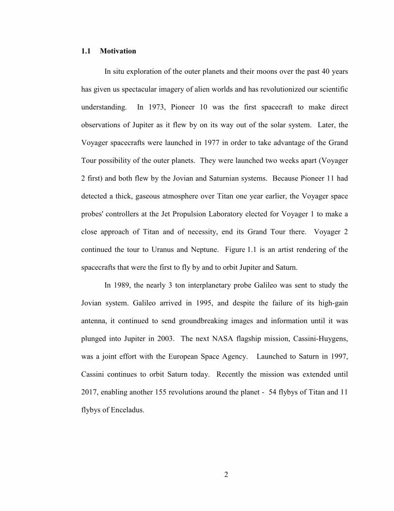
Figure 1.1. Past Missions to the outer planets. Pioneer (1973) and Voyager
(1979) were the first to fly by Jupiter and Saturn, respectively.
Galileo orbited Jupiter from 1995 to 2003 and returned wonderful
data on the whole system. Cassini-Huygens was launched in 2004
and continues to send invaluable data on the Saturnian system,
including Titan........................................................................................... 3
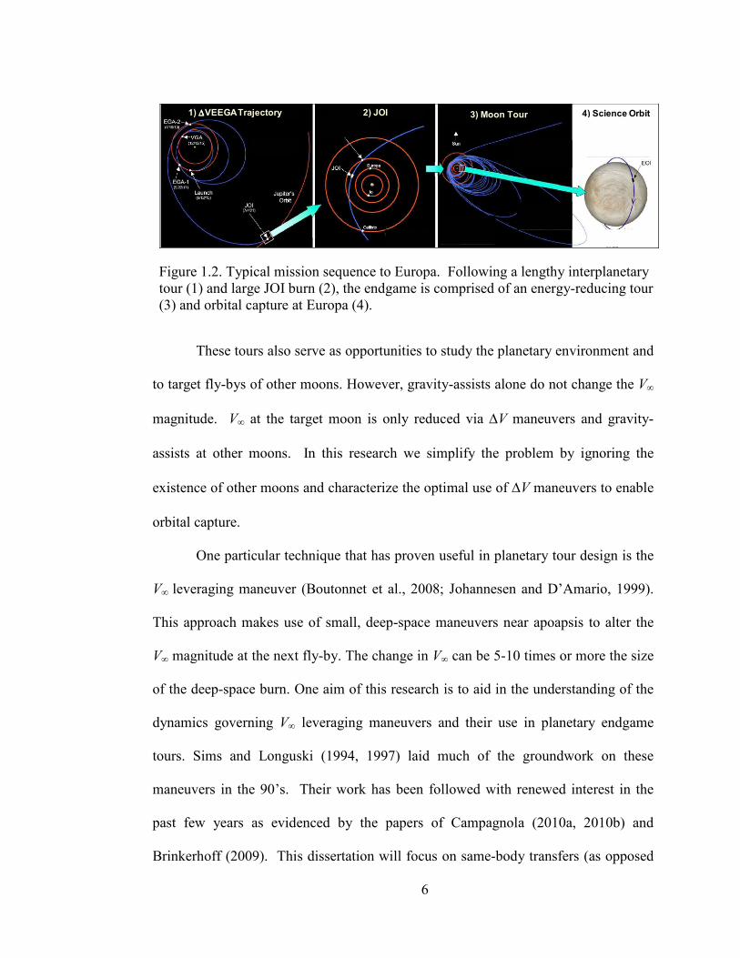
Figure 1.2. Typical mission sequence to Europa. Following a lengthy
interplanetary tour (1) and large JOI burn (2), the endgame is
comprised of an energy-reducing tour (3) and orbital capture at
Europa (4). ................................................................................................. 6
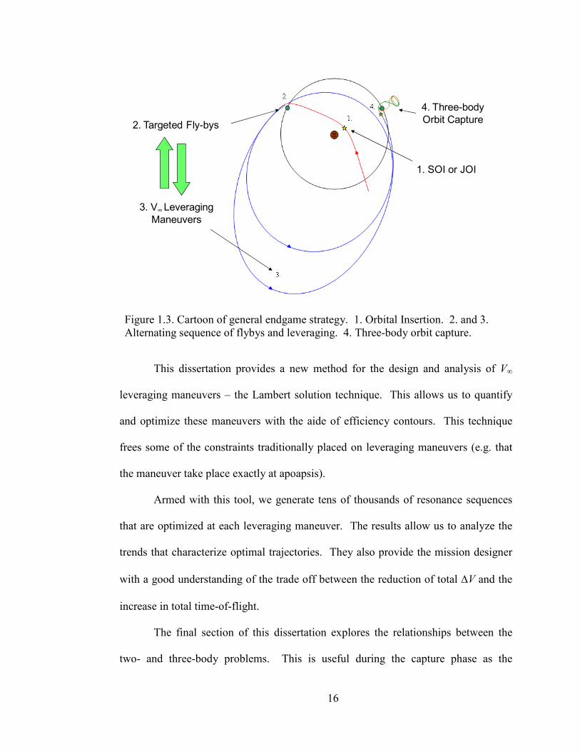
Figure 1.3. Cartoon of general endgame strategy. 1. Orbital Insertion. 2. and 3.
Alternating sequence of flybys and leveraging. 4. Three-body orbit
capture...................................................................................................... 16
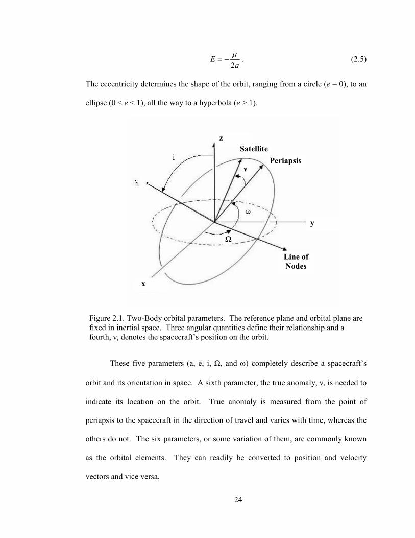
Figure 2.1. Two-Body orbital parameters. The reference plane and orbital plane
are fixed in inertial space. Three angular quantities define their
relationship and a fourth, ν, denotes the spacecraft’s position on the
orbit.......................................................................................................... 24
xiv
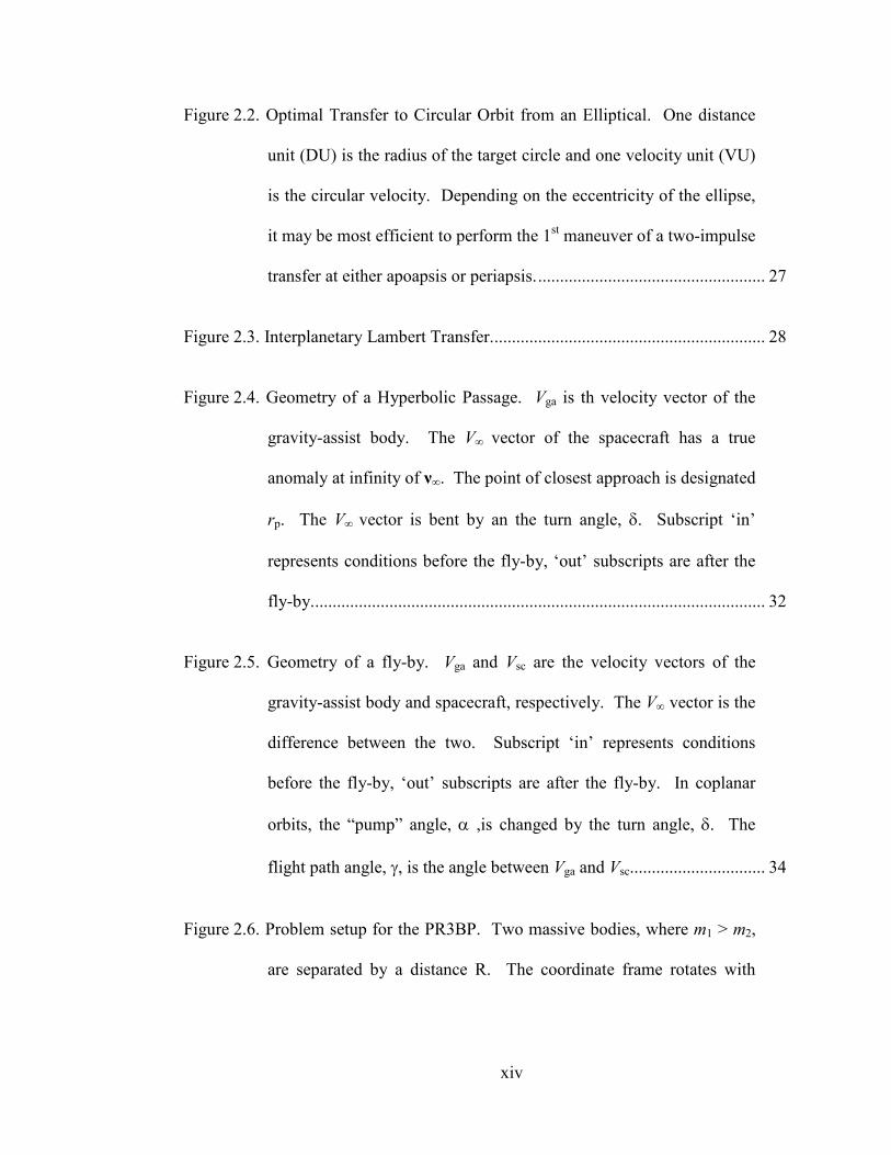
Figure 2.2. Optimal Transfer to Circular Orbit from an Elliptical. One distance
unit (DU) is the radius of the target circle and one velocity unit (VU)
is the circular velocity. Depending on the eccentricity of the ellipse,
it may be most efficient to perform the 1st maneuver of a two-impulse
transfer at either apoapsis or periapsis..................................................... 27
Figure 2.3. Interplanetary Lambert Transfer............................................................... 28
Figure 2.4. Geometry of a Hyperbolic Passage. Vga is th velocity vector of the
gravity-assist body. The V∞ vector of the spacecraft has a true
anomaly at infinity of ν∞. The point of closest approach is designated
rp. The V∞ vector is bent by an the turn angle, δ. Subscript ‘in’
represents conditions before the fly-by, ‘out’ subscripts are after the
fly-by........................................................................................................ 32
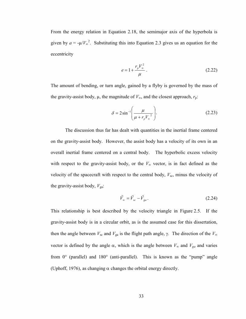
Figure 2.5. Geometry of a fly-by. Vga and Vsc are the velocity vectors of the
gravity-assist body and spacecraft, respectively. The V∞ vector is the
difference between the two. Subscript ‘in’ represents conditions
before the fly-by, ‘out’ subscripts are after the fly-by. In coplanar
orbits, the “pump” angle, α ,is changed by the turn angle, δ. The
flight path angle, γ, is the angle between Vga and Vsc............................... 34
Figure 2.6. Problem setup for the PR3BP. Two massive bodies, where m1 > m2,
are separated by a distance R. The coordinate frame rotates with
xv
angular velocity ω about their barycenter. A small third body, m3,
moves in their vicinity. ............................................................................ 39
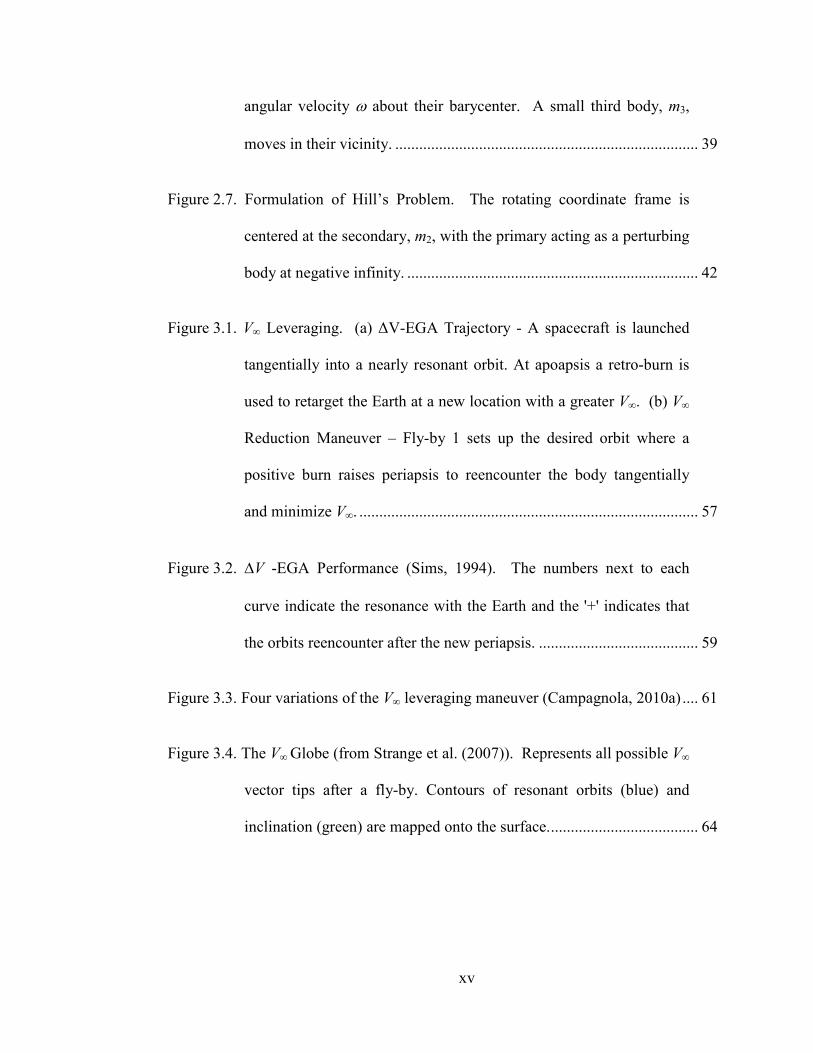
Figure 2.7. Formulation of Hill’s Problem. The rotating coordinate frame is
centered at the secondary, m2, with the primary acting as a perturbing
body at negative infinity. ......................................................................... 42
Figure 3.1. V∞ Leveraging. (a) ∆V-EGA Trajectory - A spacecraft is launched
tangentially into a nearly resonant orbit. At apoapsis a retro-burn is
used to retarget the Earth at a new location with a greater V∞. (b) V∞
Reduction Maneuver – Fly-by 1 sets up the desired orbit where a
positive burn raises periapsis to reencounter the body tangentially
and minimize V∞. ..................................................................................... 57
Figure 3.2. ∆V -EGA Performance (Sims, 1994). The numbers next to each
curve indicate the resonance with the Earth and the '+' indicates that
the orbits reencounter after the new periapsis. ........................................ 59
Figure 3.3. Four variations of the V∞ leveraging maneuver (Campagnola, 2010a) .... 61
Figure 3.4. The V∞ Globe (from Strange et al. (2007)). Represents all possible V∞
vector tips after a fly-by. Contours of resonant orbits (blue) and
inclination (green) are mapped onto the surface...................................... 64
xvi
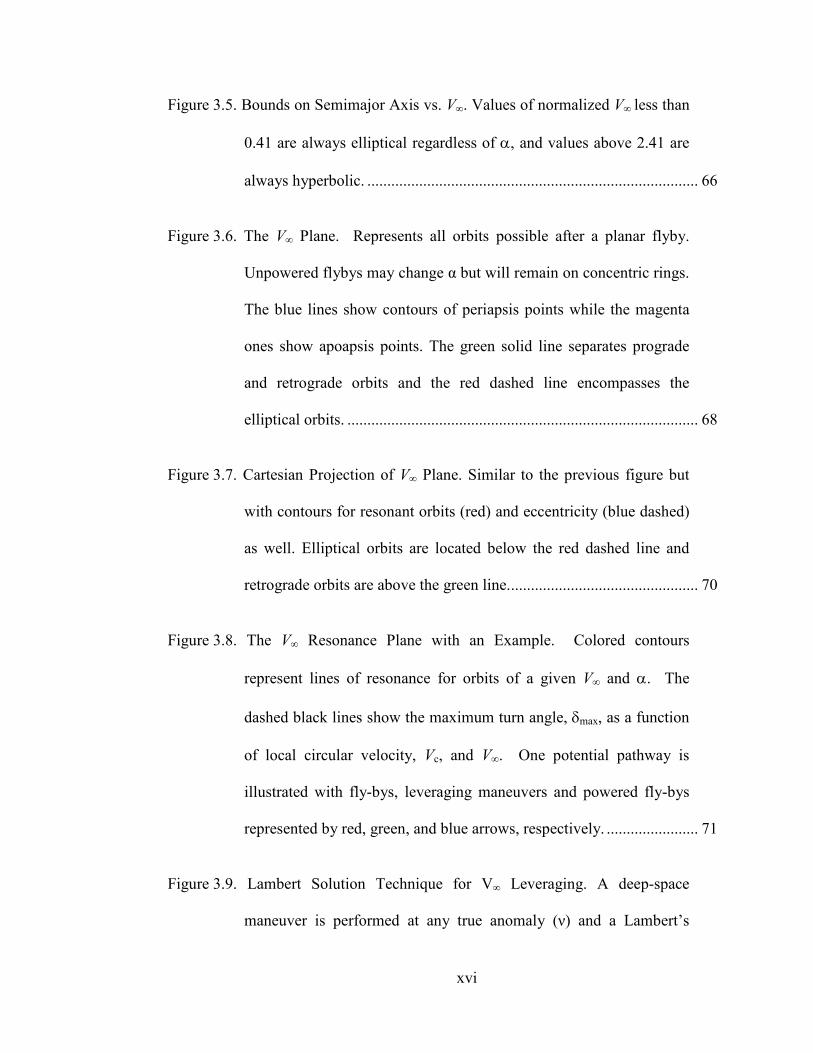
Figure 3.5. Bounds on Semimajor Axis vs. V∞. Values of normalized V∞ less than
0.41 are always elliptical regardless of α, and values above 2.41 are
always hyperbolic. ................................................................................... 66
Figure 3.6. The V∞ Plane. Represents all orbits possible after a planar flyby.
Unpowered flybys may change α but will remain on concentric rings.
The blue lines show contours of periapsis points while the magenta
ones show apoapsis points. The green solid line separates prograde
and retrograde orbits and the red dashed line encompasses the
elliptical orbits. ........................................................................................ 68
Figure 3.7. Cartesian Projection of V∞ Plane. Similar to the previous figure but
with contours for resonant orbits (red) and eccentricity (blue dashed)
as well. Elliptical orbits are located below the red dashed line and
retrograde orbits are above the green line................................................ 70
Figure 3.8. The V∞ Resonance Plane with an Example. Colored contours
represent lines of resonance for orbits of a given V∞ and α. The
dashed black lines show the maximum turn angle, δmax, as a function
of local circular velocity, Vc, and V∞. One potential pathway is
illustrated with fly-bys, leveraging maneuvers and powered fly-bys
represented by red, green, and blue arrows, respectively. ....................... 71
Figure 3.9. Lambert Solution Technique for V∞ Leveraging. A deep-space
maneuver is performed at any true anomaly (ν) and a Lambert’s

xvii
solver is used to determine the direction and magnitude to retarget
the body at any location (θ). .................................................................... 73
Figure 3.10. Efficiency of V∞ Leveraging near 2:1 Resonance. ν is the location of
the burn and θ is the location of reencounter. a) Efficiencies for 2:1 –
note that there are two peaks, with the largest being for -θ. b)
Efficiencies for 1.99:1. c) Efficiencies for 2.01:1 ................................... 75
Figure 3.11. (a) Leveraging efficiencies around 2:1 resonance, (b)-(d) The ∆V∞’s,
ν’s, and θ’s associated with the peak efficiencies in (a). ........................ 76
Figure 3.12. Expanded view of efficiencies (a) and ∆V∞ (b) near 2:1. Numerical
difficulties occur around the integer resonance, causing the location
of the efficiencies to jump to another region. .......................................... 77
Figure 3.13. Efficiencies of orbits with K:1 resonances along with their peak
values. ...................................................................................................... 78
Figure 3.14. Leveraging Efficiencies around 3:2. The blue lines are 3:2(1) and
red are 3:2(2). While it appears that maneuvers performed on the first
orbit are more efficient (a), 2nd orbit maneuvers have a greater
change in V∞ (b) and may be preferable in some instances. .................... 79
Figure 3.15. a) Efficiencies for K:1 (blue), K:2 (red), and K:3 (green) resonances.
The peak efficiencies fall on a line indicating the relationship
xviii
between resonance and efficiency, given by linear fit. b) ∆ V∞ goes
towards zero at each point of maximum efficiency................................. 80
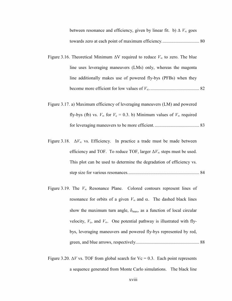
Figure 3.16. Theoretical Minimum ∆V required to reduce V∞ to zero. The blue
line uses leveraging maneuvers (LMs) only, whereas the magenta
line additionally makes use of powered fly-bys (PFBs) when they
become more efficient for low values of V∞............................................ 82
Figure 3.17. a) Maximum efficiency of leveraging maneuvers (LM) and powered
fly-bys (fb) vs. V∞ for Vc = 0.3. b) Minimum values of V∞ required
for leveraging maneuvers to be more efficient. ....................................... 83
Figure 3.18. ∆V∞ vs. Efficiency. In practice a trade must be made between
efficiency and TOF. To reduce TOF, larger ∆V∞ steps must be used.
This plot can be used to determine the degradation of efficiency vs.
step size for various resonances............................................................... 84
Figure 3.19. The V∞ Resonance Plane. Colored contours represent lines of
resonance for orbits of a given V∞ and α. The dashed black lines
show the maximum turn angle, δmax, as a function of local circular
velocity, Vc, and V∞. One potential pathway is illustrated with fly-
bys, leveraging maneuvers and powered fly-bys represented by red,
green, and blue arrows, respectively........................................................ 88
Figure 3.20. ∆V vs. TOF from global search for Vc = 0.3. Each point represents
a sequence generated from Monte Carlo simulations. The black line
xix
represents a Pareto front comprised of the most efficient sequences.
Note the rapid drop in ∆V for the shorter TOFs followed by a
flattening after about 5 time units. ........................................................... 91
Figure 3.21. Pareto front broken into the 3 overarching rules for Vc = 0.2: NX –
Sequences do not cross the δmax line (α always returns to zero), PH –
Phasing orbits are used when α > δmax, NT – Non-tangent orbits are
used when α > δmax. ................................................................................. 95
Figure 3.22. Pareto fronts for various values of Vc.................................................... 96
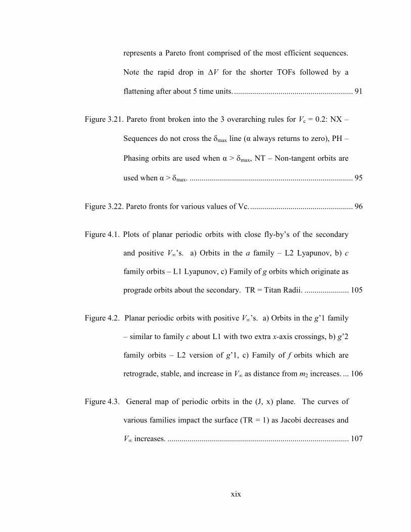
Figure 4.1. Plots of planar periodic orbits with close fly-by’s of the secondary
and positive V∞’s. a) Orbits in the a family – L2 Lyapunov, b) c
family orbits – L1 Lyapunov, c) Family of g orbits which originate as
prograde orbits about the secondary. TR = Titan Radii. ...................... 105
Figure 4.2. Planar periodic orbits with positive V∞’s. a) Orbits in the g’1 family
– similar to family c about L1 with two extra x-axis crossings, b) g’2
family orbits – L2 version of g’1, c) Family of f orbits which are
retrograde, stable, and increase in V∞ as distance from m2 increases. ... 106
Figure 4.3. General map of periodic orbits in the (J, x) plane. The curves of
various families impact the surface (TR = 1) as Jacobi decreases and
V∞ increases. .......................................................................................... 107
xx
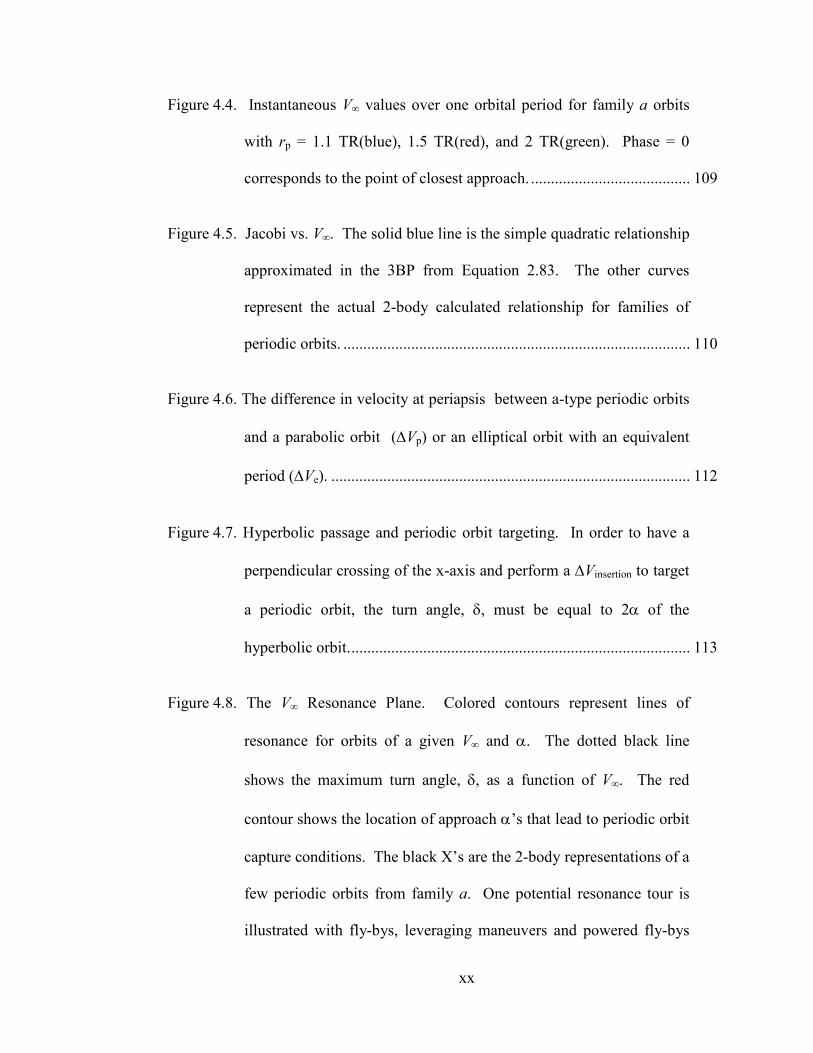
Figure 4.4. Instantaneous V∞ values over one orbital period for family a orbits
with rp = 1.1 TR(blue), 1.5 TR(red), and 2 TR(green). Phase = 0
corresponds to the point of closest approach. ........................................ 109
Figure 4.5. Jacobi vs. V∞. The solid blue line is the simple quadratic relationship
approximated in the 3BP from Equation 2.83. The other curves
represent the actual 2-body calculated relationship for families of
periodic orbits. ....................................................................................... 110
Figure 4.6. The difference in velocity at periapsis between a-type periodic orbits
and a parabolic orbit (∆Vp) or an elliptical orbit with an equivalent
period (∆Ve). .......................................................................................... 112
Figure 4.7. Hyperbolic passage and periodic orbit targeting. In order to have a
perpendicular crossing of the x-axis and perform a ∆Vinsertion to target
a periodic orbit, the turn angle, δ, must be equal to 2α of the
hyperbolic orbit...................................................................................... 113
Figure 4.8. The V∞ Resonance Plane. Colored contours represent lines of
resonance for orbits of a given V∞ and α. The dotted black line
shows the maximum turn angle, δ, as a function of V∞. The red
contour shows the location of approach α’s that lead to periodic orbit
capture conditions. The black X’s are the 2-body representations of a
few periodic orbits from family a. One potential resonance tour is
illustrated with fly-bys, leveraging maneuvers and powered fly-bys
xxi
represented by red, green, and blue arrows, respectively. The dotted
blue arrow shows a direct insertion maneuver to a parabolic orbit,
whereas the dashed red and blue arrows show an alternative approach
and capture to a hyperbolic periodic orbit. ............................................ 114
Figure 9.1. Universal variables solution regions for Lambert’s problem. ................ 136
Figure 9.2. Type III inbound (red) and outbound (green) transfer trajectories......... 137
1
1 Introduction
The Cassini-Huygens spacecraft entered orbit about Saturn on July 1, 2004.
On Christmas day of that year, the Huygens probe was released and made its way
towards the surface of Titan. The data sent back from Huygens and Cassini about this
amazing moon were nothing short of astounding. They revealed an icy world with
methane seas and a thick organic haze, with rugged shorefronts and winding canyons.
Scientific interest in Titan exploded and the community called for plans to send a
dedicated orbiter.
Missions being studied by the National Aeronautics and Space Administration
(NASA) at the time (e.g. Titan Explorer) required the use of aerocapture, an unproven
technology, to enable a spacecraft to enter orbit about Titan. Studies had shown that
aerocapture would allow 2.4 times as much mass to be delivered when compared to
an all-propulsive trajectory (Edwards, 2005). However, in 2007, it was decided that
aerocapture was too great of a risk, both technologically and in cost, to be included in
baseline architectures. The problem of how to minimize the fuel requirements of a
chemical trajectory to a Titan orbit in order to enable a mission without aerocapture
became the impetus for this research.
2
1.1 Motivation
In situ exploration of the outer planets and their moons over the past 40 years
has given us spectacular imagery of alien worlds and has revolutionized our scientific
understanding. In 1973, Pioneer 10 was the first spacecraft to make direct
observations of Jupiter as it flew by on its way out of the solar system. Later, the
Voyager spacecrafts were launched in 1977 in order to take advantage of the Grand
Tour possibility of the outer planets. They were launched two weeks apart (Voyager
2 first) and both flew by the Jovian and Saturnian systems. Because Pioneer 11 had
detected a thick, gaseous atmosphere over Titan one year earlier, the Voyager space
probes' controllers at the Jet Propulsion Laboratory elected for Voyager 1 to make a
close approach of Titan and of necessity, end its Grand Tour there. Voyager 2
continued the tour to Uranus and Neptune. Figure 1.1 is an artist rendering of the
spacecrafts that were the first to fly by and to orbit Jupiter and Saturn.
In 1989, the nearly 3 ton interplanetary probe Galileo was sent to study the
Jovian system. Galileo arrived in 1995, and despite the failure of its high-gain
antenna, it continued to send groundbreaking images and information until it was
plunged into Jupiter in 2003. The next NASA flagship mission, Cassini-Huygens,
was a joint effort with the European Space Agency. Launched to Saturn in 1997,
Cassini continues to orbit Saturn today. Recently the mission was extended until
2017, enabling another 155 revolutions around the planet - 54 flybys of Titan and 11
flybys of Enceladus.
3
3
Figure 1.1. Past Missions to the outer planets. Pioneer (1973) and Voyager (1979) were the first to fly by Jupiter and Saturn, respectively. Galileo orbited Jupiter from 1995 to 2003 and returned wonderful data on the whole system. Cassini-Huygens was launched in 2004 and continues to send invaluable data on the Saturnian system, including Titan.
NASA has sanctioned dozens of studies for over a decade to determine the
next flagship mission (> $1B) to follow Galileo and Cassini. Some examples include
Europa Orbiter, JIMO, and the Titan Explorer. The Outer Planets Assessment Group
(OPAG) was established by NASA in late 2004 to identify scientific priorities and
pathways for exploration in the outer solar system. The group consists of a 15-person
steering committee, which actively solicits input from the scientific community and
reports its findings to NASA Headquarters. OPAG has held numerous meetings to
determine scientific benefits and technological feasibility for dedicated missions to
most of the outer planets.
4
In 2007-2008 NASA and ESA put forth various concepts for missions to
Saturn and Jupiter. In February 2009, NASA and ESA officials selected the Europa
Jupiter System Mission (EJSM) as the next Outer Planet Flagship Mission, but it was
also decided to continue pursuing another potential mission to the Saturnian system.
Both missions require the delivery of large payloads to useful scientific orbits about
planetary moons, a task that can require an excessive amount of fuel if the trajectory
and implementation are not carefully and cleverly planned.
This dissertation makes extensive use of normalized quantities and
generalizing assumptions so as to make the results applicable to any three-body
system and not just the Saturn-Titan System. The hope is that the principles and
concepts set forth in this research will aide in the global effort to explore the many
interesting moons of the solar system.
1.2 Problem Characterization
The final phase of a trajectory to a science orbit is known as the “endgame.”
This phase is very challenging and often tedious for mission designers (Sweetser et
al., 1997). Typical science orbits require close proximity to the surface and high
inclinations to provide global coverage for mapping purposes. These orbits are very
costly (fuel-wise) to achieve via direct insertion. Furthermore, since delivering the
desired scientific payloads requires large amounts of fuel, missions are limited by
launch vehicle capabilities. There are a variety of techniques and tools available to
5
aide in the reduction of the total required ∆V1. Recently much work has been done to
determine how to optimally apply these techniques to meet mission requirements and
to minimize manual effort (Sims et al., 1997; Ross and Grover, 2007a; Brinckerhoff
and Russell, 2009; Campagnola and Russell, 2010a; Ross and Scheeres, 2007;
Casalino et al., 1998).
In practice, missions to planetary moons such as Europa and Titan employ the
use of extensive tours with multiple gravity-assists in order to reduce hyperbolic
excess velocity2 (hereafter referred to as V∞) at the final moon encounter, enabling a
feasible orbit insertion. Figure 1.2 shows the trajectory of the Europa Explorer
(Clark, et al., 2007). The mission begins with a flyby of Venus and two at Earth en
route to Jupiter. Upon arrival, a flyby of Callisto is used to lower the fuel needed for
the large Jupiter orbit insertion (JOI) burn. Following capture in the Jovian system,
the spacecraft begins a tour of highly elliptical orbits using flybys of the massive
moons to remove orbital energy and to set up the final insertion at Europa. The
energy-reducing tour and final capture (steps 3 and 4 in Figure 1.2) make up the
“endgame”.
1 The cost of impulsive maneuvers can be expressed in terms of mass, but this measure is dependent on the dry mass of the spacecraft and the efficiency (Isp) of the engine. Instead, it is more common to express the effects of impulsive maneuvers in terms of the magnitude of the change in velocity they
produce, known as ∆V, which can be used as a surrogate for fuel usage. _ 2 See Appendix A: Nomenclature at the end of this dissertation for a description of symbols used
6
1) ∆∆∆∆VEEGA Trajectory 2) JOI 3) Moon Tour 4) Science Orbit
Figure 1.2. Typical mission sequence to Europa. Following a lengthy interplanetary tour (1) and large JOI burn (2), the endgame is comprised of an energy-reducing tour (3) and orbital capture at Europa (4).
These tours also serve as opportunities to study the planetary environment and
to target fly-bys of other moons. However, gravity-assists alone do not change the V∞
magnitude. V∞ at the target moon is only reduced via ∆V maneuvers and gravity-
assists at other moons. In this research we simplify the problem by ignoring the
existence of other moons and characterize the optimal use of ∆V maneuvers to enable
orbital capture.
One particular technique that has proven useful in planetary tour design is the
V∞ leveraging maneuver (Boutonnet et al., 2008; Johannesen and D’Amario, 1999).
This approach makes use of small, deep-space maneuvers near apoapsis to alter the
V∞ magnitude at the next fly-by. The change in V∞ can be 5-10 times or more the size
of the deep-space burn. One aim of this research is to aid in the understanding of the
dynamics governing V∞ leveraging maneuvers and their use in planetary endgame
tours. Sims and Longuski (1994, 1997) laid much of the groundwork on these
maneuvers in the 90’s. Their work has been followed with renewed interest in the
past few years as evidenced by the papers of Campagnola (2010a, 2010b) and
Brinkerhoff (2009). This dissertation will focus on same-body transfers (as opposed
7
to multi-moon tours) where only one body is used during the endgame. We will also
confirm some of the findings of the research mentioned above. The results are
presented with the mission designer in mind who wishes to quickly evaluate the
possibilities and trade space before moving to a more detailed trajectory.
In order to better visualize the optimization of the endgame design process,
we propose the use of a three-dimensional “V∞ Sphere” as a guide map. This map is
based on the “V∞ Globe”3 as proposed by Strange and Russell (2007). As spacecraft
maneuvers are performed the magnitude of the V∞ vector, which will later be shown
to be analogous to the Jacobi constant, is modified. Strategically placed maneuvers
will reduce the size of the V∞ Globe at the next encounter, which can be thought of as
the next layer of the V∞ Sphere. The contours delineating post fly-by orbit parameters
on the surface of the V∞ Globe trace out three-dimensional surfaces as the size of the
sphere shrinks. Getting to the center of this sphere using the minimal amount of fuel
is the ultimate goal of the endgame design process.
Traditional planetary capture methods require that this V∞ Sphere be reduced
to zero, which is not possible using fly-bys alone. With the additional use of V∞
leveraging maneuvers, it is possible to greatly reduce the amount of fuel required to
bring down the V∞ magnitude and ultimately capture into an orbit about the body.
With the V∞ Sphere providing a map for potential orbit sequences, the problem
becomes how to optimally shrink the sphere. V∞ leveraging maneuvers are typically
performed at the spacecraft's apoapsis and tangent to the orbit. Sweetser (1993)
3 We will use the term “globe” to denote a surface, whereas “sphere” is used to denote the entire 3-
dimensional object.
8
showed that this maximizes the change in Jacobi constant. However, our numerical
investigations have shown that this is slightly suboptimal due to the targeting
restraints when solving Lambert's problem.
In the 2-body problem (2BP), V∞ at the target moon is a constant in the
absence of perturbations or leveraging maneuvers, much like the Jacobi constant in
the 3-body problem (3BP). Since gravity assists and the transition to gravitational
capture are essentially expressions of third body effects, it makes more sense to
analyze them using three-body techniques. In the patched 2BP, V∞ = 0 corresponds to
a parabolic orbit or the limit of gravitational capture. Relationships between the
Jacobi and V∞ yield the possibility of bound, periodic, or quasi-periodic orbits with a
positive V∞. If such orbits exist, then they would amount to hyperbolic orbits in the
2-body sense yet be bound to the vicinity of the secondary. Targeting a “hyperbolic
periodic” orbit during the final phase of a leveraging maneuver sequence would result
in a lower required insertion ∆V. After a spacecraft has been inserted on to a periodic
capture orbit, it may be required to then transfer to a low science orbit, which is
beyond the scope of this dissertation. It is noted, however, that much research has
been done on these types of transfers (see Davis (2009) and Russell (2006)).
1.3 Historical Roots
The purpose of this section is to provide a brief history of previous work in
astrodynamics that has lead to modern day mission design and to show the
background leading up to this dissertation.
9
1.3.1 A Brief History of Two-Body Problem
Great minds throughout the ages have been interested in the celestial motions
they observed in the night sky. In 1601, Johannes Kepler became the director of the
Prague Observatory following the death of Tycho Brahe. Using Brahe’s meticulously
collected data, Kepler formulated his famous three laws of planetary motion:
1) Every planet moves in an elliptical orbit, with the sun at one focus.
2) The radius vector sweeps out equal areas in equal times.
3) The square of the period is proportional to the cube of the semimajor axis.
Later that century, Newton (1687) would go on to devise his three laws of motion and
put forth his theory of gravitation:
2
21
r
mGmF = (1.1)
where G is the universal gravitational constant and r is the distance between mass 1
(m1) and mass 2 (m2). Armed with his newly invented calculus and laws of
gravitation, Newton set out to explain Kepler’s laws. He succeeded in
mathematically and geometrically describing the laws that govern planetary motion
and derived many of the equations that are used today.
In 1744, Leonhard Euler went on to find the full analytical solution to the two-
body equations. He was also one of the first to derive the equations defining the
change in osculating elements with time, giving rise to the analytic theory of
perturbed motions (Euler, 1744). In works published in 1761 and 1771, Johann
Lambert used a geometrical approach to generalize Euler’s formulas to include
elliptical and hyperbolic orbits. Therefore, solving for the orbit between two known
position vectors is usually known as Lambert’s problem (see 2.1.3). General
10
understanding of orbit determination in the 2BP was further enhanced by the works of
Lagrange (1778), Laplace (1880), and Gauss (1802).
One of the most well known transfers in the two-body problem is the
Hohmann transfer. Hohmann (1925) proposed a theory which suggests that the
minimum cost transfer between two circular orbits, in terms of fuel expenditure, can
be achieved by employing two burns: the first maneuver is tangential to the initial
orbit, and the second maneuver is tangential to the final orbit. The Hohmann transfer
represents the minimum change in velocity between most coplanar orbits.
1.3.2 A Brief History of the Three-Body Problem
The 3BP is a classic problem of celestial mechanics, wherein we are interested
in the motion of a third particle in the presence of two massive bodies. One of the
earliest contributors to the 3BP was Sir Isaac Newton (1687), in the years after he
published his theory of gravitation. The problem of ocean navigation required an
understanding of the motion of the Moon, which is strongly affected by both the
Earth and the Sun and, hence, beyond the scope of the basic 2BP. This problem was
of great interest throughout the eighteenth century and was approached in basically
two ways: by an infinite series expansion to describe the solution (Clairaut, 1752) or
by variation of parameters (Euler, 1744). It was Euler who first used rotating
coordinates to frame the problem. However, it was not until 1772 that Lagrange
(1867-1892) demonstrated a reduction of the problem from its original form, with 18
unknowns, to a problem of order 7 in the rotating frame. Lagrange proposed the
assumptions that lead to the “restricted” model, allowing closed form solutions and
more detailed analyses of celestial motions (Barrow-Green, 1997).
11
It was also Lagrange who first identified the five equilibrium points in the
circularly restricted three-body problem (CR3BP): the three collinear points (which
were also described by Euler in 1772) and two equilateral points. This is why they
are usually denoted the Lagrange points.
The next significant contribution to the 3BP did not appear until Carl Jacobi in
1836. He discovered the only integral of the motion in the CR3BP, which bears his
name as the Jacobi Constant. Jacobi's work was further extended by Hill (1878) who
used this lone integral to define curves of zero velocity that limit the motion of the
third particle. Hill's investigations focused on the Moon and, thus, constrained the
Moon's motion to certain regions of space around the two main bodies (the Sun and
the Earth).
Another significant step in understanding the three-body problem came about
due to a mathematical competition to honor the 60th birthday King Oscar II of
Sweden and Norway in 1889. Henri Poincaré was awarded the prize for his study of
the CR3BP. What set his work apart was that he shifted from a quantitative aspect to
a more qualitative assessment. While Poincaré (1890) was interested in finding
solutions to the three-body problem, his approach differed from all previous
developments, since he was more interested in the nature of the solutions than in the
actual solutions themselves. His mathematical work showed that an infinite number
of periodic orbits exist in the 3BP. Poincaré also introduced an innovative method,
the Poincaré section (or stroboscopic map) to study the behavior of solutions as time
tends to infinity (Barrow-Green, 1997). Poincaré is considered by many to be the
father of dynamical systems theory.
12
Around the turn of the century, there was much work being done in the field
of dynamical systems theory. Tisserand (1896) used it to study and identify comets
and their orbits. Lyapunov (1892) and Levi-Civita (1901), were interested in a more
general theory of the stability of motion, and in the case of Levi-Civita, its application
to the CR3BP. Their work laid the foundation for modern efforts to compute the
invariant manifolds associated with periodic orbits in the 3BP. Other notable
researchers in the areas of periodic orbits and general solutions include Darwin (1897,
1911), Sundman (1912), and Strömgren (1935).
Continuing advancements in the determination of periodic orbits and the
advent of modern computers and technology led to the launch of the ISEE-3
spacecraft in 1978 (Farquhar, 1998). It was the first spacecraft to be inserted into a
halo orbit in the vicinity of the L1 Sun-Earth libration point. Since then many
spacecraft have benefited from orbits determined by dynamical systems theory,
including SOHO, ACE, and Genesis. Other researchers that have contributed
significantly to the understanding of periodic orbits include Hénon (1965-1970),
Szebehely (1967), and Broucke (1968).
1.3.3 Recent Related Work
In the past few decades, many new techniques have been developed in support
of missions to the outer planets and their moons. In the late 1990’s and early 2000’s,
a multitude of papers were published concerning mission designs to Europa and other
moons of Jupiter. Most of these were in support of the Europa Orbiter or Jupiter Icy
Moons Orbiter (JIMO) missions. In 1997, Ted Sweetser and others spelled out “a
plethora of astrodynamic challenges” facing trajectory design for a Europa Orbiter.
13
Mission designers and theorists alike set to work tackling these problems incumbent
upon sending an orbiter to a small planetary moon.
The first challenge facing designers was the daunting task of finding a tour
design that reduced the Jovicentric energy while simultaneously meeting all the other
mission criteria. In 1999, Johannesen and D’Amario of JPL published the reference
trajectory of the Europa Orbiter, which was the baseline for most studies of the day.
However, this was only a point design4 and inflexible to schedule or requirement
changes. Heaton and others at Purdue set to work on an automated process that took
in constraints on total time of flight and radiation dosage (Heaton, et al., 2000). They
found an enormous number of possible sequences and documented the most
promising.
The dynamics of the multi-moon environment lends itself well to optimization
techniques and the application of dynamical systems theory. A number of researchers
tackled this problem including Ross and Grover (2007b), who looked at low thrust
and multiple gravity-assists to navigate the unstable manifolds on near-ballistic
trajectories, with the aid of Keplerian maps. Papers by Strange and Longuski (2002)
and Strange, Russell, and Buffington (2007) also put forth graphical methods for the
design of tours with gravity-assists, including the V∞ Globe (see Section 3.3).
Another problem identified early on was the stability of suitable science
orbits. Scheeres, Guman, and Villac (2000, 2001) studied orbital stability using
numerical and analytical techniques. They found that impact orbits only occur within
~45° of a polar orbit, but with certain initial conditions, impact can be delayed for a
4 The launch date for Europa Orbiter was set for 2003.
14
considerable length of time. Gomez, Lara, and Russell (2006) took a dynamical
systems approach to find orbits that were stable and met mission criteria by using
averaged manifolds of unstable frozen orbits. Achieving these low orbits directly
using an insertion maneuver is often very costly, fuel-wise. That is why Russell and
Lam (2005, 2006) looked in to the use of unstable, periodic orbits as an intermediate
capture mechanism. This idea of using quasi-periodic orbits for orbital capture was
also studied by Nakamiya, et al. (2007), with applications to periodic orbits about
libration points.
Most recently, the well established technique of V∞ leveraging has been
applied to the planetary moon tour problem (Brinkerhoff and Russell, 2009). Used in
conjunction with resonant gravity-assists, it becomes a pathfinding problem to find
optimal tour sequences. Campagnola and Russell (2010a, 2010b) developed
Tisserand leveraging graphs and phase-free formulae in order to analyze the endgame
to the multi-body gravity-assist problem. Their results help find the minimum ∆V
transfers between two moons and have been applied to enable an Enceladus5 orbiter
(Strange et al, 2009a; Campagnola et al., 2010c).
1.4 Contributions of This Dissertation
As shown by the previous section, much work has been done that is applicable
to mission design of planetary moon orbiters. However, some techniques are
developed as solutions to very specific, mathematically interesting problems. These
theoretical discoveries can be quite clever, but fail to be implemented in the practical
5 Enceladus is difficult to orbit in that it is very small and close to Saturn.
15
realm as mission designers are not given the big picture nor the tools to easily
incorporate them into their studies. Other techniques are well developed, but are only
applicable to one small phase of the problem and are difficult to mesh with other
techniques. This dissertation seeks to connect multiple techniques together so that
they can be seen as a whole. From there, mission designers will be able to quickly
assess the usefulness of techniques across the trade space.
As was mentioned previously, the tour design problem lends itself well to
optimization schemes. However, optimization schemes are only as accurate as their
inputs and often times can only provide local optima, unbeknownst to the user. In
order to avoid these pitfalls it is important to have a firm understanding of the big
picture to be able to describe the problem accurately. Most trajectory optimization
software requires the input of a relatively good initial guess. In this work we seek to
characterize the trade space and provide approximations of global minima as inputs to
high fidelity optimizers.
The cartoon in Figure 1.3 shows the stages of our overall endgame strategy.
The trajectory begins with a highly elliptical orbit following Saturn or Jupiter Orbit
Insertion (JOI). Next, an alternating sequence of targeted flybys and leveraging
maneuvers are used to reduce the V∞ at the target moon. The design of these
sequences is aided by the use of a map – the V∞ Sphere. Finally, a three-body capture
orbit is used to reduce ∆V requirement to capture to the moon’s vicinity.
16
1. SOI or JOI
2. Targeted Fly-bys
3. V∞ Leveraging
Maneuvers
4. Three-body
Orbit Capture
Figure 1.3. Cartoon of general endgame strategy. 1. Orbital Insertion. 2. and 3. Alternating sequence of flybys and leveraging. 4. Three-body orbit capture.
This dissertation provides a new method for the design and analysis of V∞
leveraging maneuvers – the Lambert solution technique. This allows us to quantify
and optimize these maneuvers with the aide of efficiency contours. This technique
frees some of the constraints traditionally placed on leveraging maneuvers (e.g. that
the maneuver take place exactly at apoapsis).
Armed with this tool, we generate tens of thousands of resonance sequences
that are optimized at each leveraging maneuver. The results allow us to analyze the
trends that characterize optimal trajectories. They also provide the mission designer
with a good understanding of the trade off between the reduction of total ∆V and the
increase in total time-of-flight.
The final section of this dissertation explores the relationships between the
two- and three-body problems. This is useful during the capture phase as the
17
transition to the target moon’s sphere of influence is better understood in the three-
body realm. We show that hyperbolic periodic orbits do exist and can be more useful
as capture mechanisms than standard two-body orbits. We also provide common
terminology and metrics that allow us seamlessly connect the capture portion of a
trajectory to the tour sequence and evaluate its usefulness.
Portions of this research have been presented at the following conferences:
1. AAS/AIAA Astrodynamics Specialist Conference, Pittsburgh,
Pennsylvania, August 2009. AAS Paper 09-377, “Shrinking the V-
infinity Sphere: Endgame Strategies for Planetary Moon Orbiters.”
2. AAS/AIAA Spaceflight Mechanics Meeting, San Diego, CA, February
2010. AAS Paper 10-219, “Optimal Pathways for Sequences of V-
infinity Leveraging Maneuvers.”
3. AAS George H. Born Symposium, Boulder, CO, May 13-14, 2010.
“Hyperbolic Periodic Orbits in the Three-Body Problem and Their
Application to Orbital Capture.”
It is also contained in the following (submitted) journal papers:
1. Woolley, R.C. and D.J. Scheeres, “Applications of V-infinity
Leveraging Maneuvers to Endgame Strategies for Planetary Moon
Orbiters,” Journal of Guidance, Control, and Dynamics, Submitted
Mar. 2010.
2. Woolley, R.C and D.J. Scheeres, “Hyperbolic Periodic Orbits in the
Three-Body Problem and Their Application to Orbital Capture,” The
Journal of the Astronautical Sciences. (Pending submission).
18
1.5 Dissertation Organization
This dissertation is organized as follows: Chapter 2 reviews the models and
methods used throughout this research. As the majority of the results are meant to
rapidly characterize a trade space and to be used for preliminary analysis, 2BP
equations are largely used. However, the transition to the sphere of influence of the
secondary during capture is better suited to the 3BP. Therefore, a discussion of the
3-body approximation and trajectory design along with the relevant equations are put
forth. The chapter is concluded with the mathematical relationship between integrals
of motion in the two- and three-body problems.
Chapter 3 describes the use of V∞ leveraging maneuvers during endgame
sequences. The V∞ Sphere, Globe, and Plane are introduced as maps of all possible
orbits resulting from same body transfers. With the aid of these maps, we tackle the
problem of finding sequences of leveraging maneuvers, flybys, and resonant orbits
that lead to V∞ = 0. A novel method for analyzing the leveraging maneuvers using a
Lambert’s solver is put forth. This method allows us to better understand the
dynamics involved in designing the most efficient maneuvers. Using maximum
efficiency plots, a theoretical minimum capture ∆V is derived.
Since the minimum also requires an infinite flight time, we then look at
feasible sequences that may be used in tour design at Saturn or Jupiter. The
combinatorics of the pathfinding problem lead to an infinite number of possible
sequences. A Monte Carlo-type simulation is used to generate tens of thousands of
19
sequences and to analyze their characteristics. It was found that it is possible to
reduce the total ∆V by 50% with only a modest increase in total time-of-flight.
Increasing the mission duration further does not result in significant reductions.
Chapter 4 looks at ways to use three-body dynamics to become captured to the
vicinity of the target moon without having to reduce V∞ to zero first. Simple periodic
orbits exist in the 3BP that are hyperbolic in the 2BP during the point of closest
approach. Using these orbits as a capture mechanism, it is possible to expend
approximately 25% less fuel during the insertion maneuver when compared to a
similar elliptical orbit.
Chapter 5 draws conclusions from this research and its applications in the
practical realm. We also suggest areas of future research that would be beneficial to
the study of endgame strategies.
20
2 Models and Methods
In order to perform analyses of endgame strategies, this dissertation makes use
of the equations of motion from the Two-Body model and the Circular Restricted
Three-Body model. The Two-Body model is used for analyzing the motion of a
spacecraft in the presence of one massive body and excludes any other perturbations.
It is accurate under the assumptions listed in Section 2.1 and can be “patched”
together to simulate trajectories with multiple bodies. It is the primary model used in
the analysis in Chapter 3. The Circular Restricted Three-Body model assumes two
massive bodies in circular orbits about their common barycenter. This approximates
most planets and moons in our solar system quite well. The augmented equations of
motion in this model allow for more complex orbits and it is the model used for
analyses in Chapter 4.
2.1 The Two-Body Problem
The two-body problem (2BP) is the starting point for nearly all reference
books in the field of astrodynamics. The basic problem describes the motion of two
point-masses in mutual gravitational attraction. It is very well suited for quick
approximations of trajectories in practical applications (including this dissertation) as
most celestial bodies are spherically symmetric and the gravitational forces of one
21
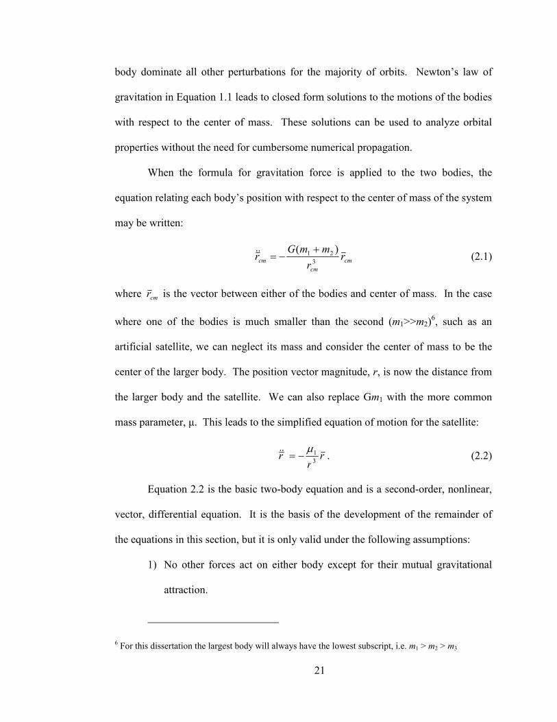
body dominate all other perturbations for the majority of orbits. Newton’s law of
gravitation in Equation 1.1 leads to closed form solutions to the motions of the bodies
with respect to the center of mass. These solutions can be used to analyze orbital
properties without the need for cumbersome numerical propagation.
When the formula for gravitation force is applied to the two bodies, the
equation relating each body’s position with respect to the center of mass of the system
may be written:
cm
cm
cm rr
mmGr
3
21 )( +−=&& (2.1)
where cmr is the vector between either of the bodies and center of mass. In the case
where one of the bodies is much smaller than the second (m1>>m2)6, such as an
artificial satellite, we can neglect its mass and consider the center of mass to be the
center of the larger body. The position vector magnitude, r, is now the distance from
the larger body and the satellite. We can also replace Gm1 with the more common
mass parameter, µ. This leads to the simplified equation of motion for the satellite:
rr
r3
1µ−=&& . (2.2)
Equation 2.2 is the basic two-body equation and is a second-order, nonlinear,
vector, differential equation. It is the basis of the development of the remainder of
the equations in this section, but it is only valid under the following assumptions:
1) No other forces act on either body except for their mutual gravitational
attraction.
6 For this dissertation the largest body will always have the lowest subscript, i.e. m1 > m2 > m3
22
2) The bodies are spherically symmetric with uniform density and can
therefore be treated point masses.
3) The mass of the smaller body is negligible compared to the central body.
4) The coordinate system must be inertial.
Manipulating Equation 2.2 gives what is known as the trajectory equation,
which describes the shape of all two-body orbits:
)cos(1
)1( 2
νe
ear
+−
= , (2.3)
where a is the semimajor axis, e is the eccentricity, and ν is the true anomaly. It
shows that all trajectories are conic sections: circles, ellipses, parabolas, or
hyperbolas. The shape that an orbit will take, and whether it is gravitationally bound
or unbound to the central body, is determined by the specific mechanical energy.
This energy is computed by subtracting the potential energy7 from the kinetic energy:
r
vE
µ−=
2
2
, (2.4)
where v is the velocity of the satellite with respect to the central body. When energy
is positive the orbit is hyperbolic and the satellite will escape the system. If energy is
negative then the satellite is gravitationally bound and will follow an elliptical or
circular orbit. Zero energy denotes a parabolic orbit where velocity goes to zero at an
infinite distance and represents the boundary of gravitational capture.
The simplifying assumptions of the 2BP allow it to be a very well-
characterized system. One way to look at it is to consider that all particles have 6
7 Since potential energy is negative, it is actually added to kinetic, which is positve
23
degrees of freedom: 3 in position and 3 in velocity. If 6 constants, or integrals of
motion, can be defined, then the motion can be known for any given time. The 2BP
has 12 degrees of freedom, but since we assume that the first body is massive and
fixed at the barycenter, the conservation of linear momentum allows us to eliminate 6.
Conservation of energy (Equation 2.4) provides the first integral, and conservation of
angular momentum along with Kepler’s first two laws provide the remaining 5. Keep
in mind this only provides a complete solution to the relative motion of the two
bodies due to the assumptions listed above.
2.1.1 Orbital Parameters
Since we know that the angular momentum vector, h = r x v8, is constant, the
plane of the orbit is fixed in space. The r and v vectors lie in this plane which is
normal to h. Now let us define a reference plane that is fixed in inertial space. The
angle between the planes is fixed and is called the inclination, i. Two more angular
parameters define their relative orientation, as shown in Figure 2.1. The first, the
longitude of the ascending node, Ω, is the angle between the x-axis (arbitrarily
defined) and the line of nodes between the planes. The second is the argument of
periapsis, ω, which measures the angle between the line of nodes and the point of
periapsis.
The size and shape of an orbit are determined by two parameters – semimajor
axis, a, and eccentricity, e. The semimajor axis is determined by the energy of an
orbit as shown by the equation
8 v = r& , or dr/dt
24
a
E2
µ−= . (2.5)
The eccentricity determines the shape of the orbit, ranging from a circle (e = 0), to an
ellipse (0 < e < 1), all the way to a hyperbola (e > 1).
Figure 2.1. Two-Body orbital parameters. The reference plane and orbital plane are fixed in inertial space. Three angular quantities define their relationship and a fourth, ν, denotes the spacecraft’s position on the orbit.
These five parameters (a, e, i, Ω, and ω) completely describe a spacecraft’s
orbit and its orientation in space. A sixth parameter, the true anomaly, ν, is needed to
indicate its location on the orbit. True anomaly is measured from the point of
periapsis to the spacecraft in the direction of travel and varies with time, whereas the
others do not. The six parameters, or some variation of them, are commonly known
as the orbital elements. They can readily be converted to position and velocity
vectors and vice versa.
x
y
z
Satellite
Periapsis
Line of
Nodes
ν
Ω
25
2.1.2 Orbital Transfers
One of the basic goals of space exploration missions is to get from one place
to another. The mechanism for doing so is known as a transfer orbit. The most basic
and common transfer is from one circular orbit to another co-planar circular orbit. In
practice most orbits are not exactly circular nor co-planar, but the analysis of such
transfers is a good approximation of many realistic orbits.
The most fundamental and most often used transfer is known as the Hohmann
transfer. It is the most energy efficient two-impulse maneuver for transferring
between two coplanar circular orbits under most circumstances. The Hohmann
transfer ellipse is half of an orbit that is tangent to both circles at its apse line. The
periapsis and apoapsis are the radii of the inner and outer circles, respectively. The
transfer can take place in either direction, for the same total ∆V.
For the case of starting on the smaller orbit, a ∆V maneuver is required to
boost the spacecraft to the transfer ellipse. The semimajor axis of this ellipse is
simply at = ½(a1 + a2), where ‘1’ and ‘2’ represent the smaller and larger orbits,
respectively. After coasting for 180 degrees towards the outer orbit, another ∆V
maneuver is applied to boost the spacecraft’s velocity to that of the larger circular
orbit. The total ∆V required for a Hohmann transfer is given by
−−+
−−=∆
tt
Hohmannaaaaaa
V121112
2211
µµ . (2.6)
If the ratio between the outer radius and the inner radius is greater than 11.94,
it may be more efficient to use what is known as the bi-elliptic transfer. This transfer
uses two coaxial semi-ellipses which extend beyond the outer target orbit. Each of
26
the ellipses is tangent to one of the circular orbits and they are tangent to each other at
the apoapsis of both. The reasoning is that the ∆V that takes place very far from the
central body will be very small due to the decreased potential. In fact, as the apoapsis
approaches infinity the ∆V goes to zero in what is known as a bi-parabolic transfer.
These are not practical as they require an infinite amount of time. The total ∆V
required for a bi-elliptical transfer is given by
+−−
+−
+=∆ −
)1(
2)1(
1)(2
1 βββ
αα
αββαµ
aV ellipticbi . (2.7)
where α = ra/a1, β = a2/a1, and ra is the location of the distant apoapsis burn. Bi-
elliptic transfers are always more efficient than Hohmann transfers when α is greater
than 15.58, as well as for large values of β when α is greater than 11.94.
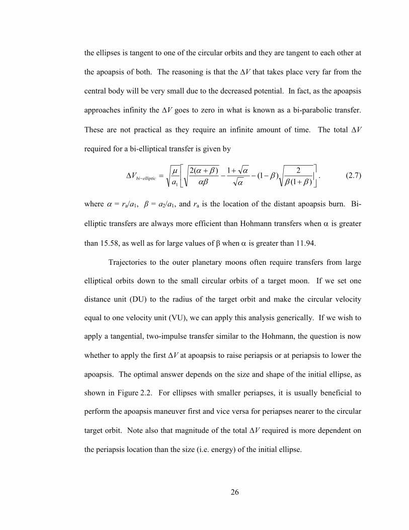
Trajectories to the outer planetary moons often require transfers from large
elliptical orbits down to the small circular orbits of a target moon. If we set one
distance unit (DU) to the radius of the target orbit and make the circular velocity
equal to one velocity unit (VU), we can apply this analysis generically. If we wish to
apply a tangential, two-impulse transfer similar to the Hohmann, the question is now
whether to apply the first ∆V at apoapsis to raise periapsis or at periapsis to lower the
apoapsis. The optimal answer depends on the size and shape of the initial ellipse, as
shown in Figure 2.2. For ellipses with smaller periapses, it is usually beneficial to
perform the apoapsis maneuver first and vice versa for periapses nearer to the circular
target orbit. Note also that magnitude of the total ∆V required is more dependent on
the periapsis location than the size (i.e. energy) of the initial ellipse.
27
0.1 0.2 0.3 0.4 0.5 0.6 0.7 0.8 0.9 11
1.5
2
2.5
3
3.5
4
0.2 0.2
0.2
0.30.3
0.3
0.3
0.4
0.4
0.4
0.4
0.5
0.5
0.5
0.5
0.6
0.6
0.6
0.6
0.7
0.7
0.7
0.7
0.8
0.8
0.8
0.9
0.9
0.9
11
1
Periapsis (DU)
Apoa
psi
s (
DU
)
1
1
1
1
1.5
1.5
1.5
2
2
2
2
Separator
Min ∆V (VU)
a
Apoapsis 1st
Periapsis 1st
Figure 2.2. Optimal Transfer to Circular Orbit from an Elliptical. One distance unit (DU) is the radius of the target circle and one velocity unit (VU) is the circular velocity. Depending on the eccentricity of the ellipse, it may be most efficient to perform the 1st maneuver of a two-impulse transfer at either apoapsis or periapsis.
2.1.3 Lambert’s Problem
According to the theorem of J. H. Lambert, the transfer time, ∆t, from one
point in space to another is independent of the orbit’s eccentricity and depends only
on the sum of the magnitudes of the position vectors, the semimajor axis, and the
length of the chord connecting the points. If we are given ∆t and two points, then
Lambert’s problem is to find the trajectory joining them. The trajectory is determined
once we find the velocity vector at the first point, because the position and velocity of
any point on an orbit are determined by r1 and v1. A proof of Lambert’s theorem is
given in Appendix C.
28
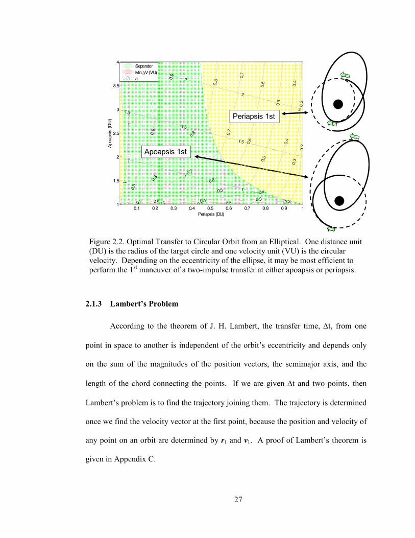
A primary application of Lambert’s problem is that of interplanetary mission
design. Known ephemeredes of the planets give the start and end positions when the
launch and arrival dates are specified. Solving Lambert’s problem defines the orbital
elements of the desired transfer orbit. It also gives the magnitude and direction of the
∆V required to achieve the transfer and to arrive at the desired orbit. Figure 2.3
shows an example of an interplanetary Lambert transfer from Earth to Mars. With
the launch and arrival dates and positions known, solving Lambert’s problem yields
the ∆V required to leave Earth orbit and to arrive at an orbit about Mars.
Figure 2.3. Interplanetary Lambert Transfer.
The time required for the transfer can be written
[ ])sin(sin2 00
3
0 EEeEEka
tt −−−+=− πµ
(2.8)
29
where k is the number of complete revolutions and E is the eccentric anomaly given
in radians. The subscript ‘0’ refer to values at the initial time. We now must find the
correct values of a, E0, E and e that will give the desired transfer time. With the latter
three parameters given by the problem definition, it only remains to find the
semimajor axis.
There are many ways to go about solving Equation 2.8 (Prussing and Conway,
1993; Schaub and Junkins, 1993), but the use of (∆E)2 allows for well-behaved
iteration and is the chosen method for the universal formulation (Battin, 1987). Such
formulation allows transfers to be elliptical, parabolic, or hyperbolic without a priori
information.
What follows is a derivation of how Lambert’s problem is solved using a
universal variables formulation. A similar derivation may be found in Bate, Mueller,
and White (1971) and Vallado (1997). For now the 2kπ term in Equation 2.8, which
is used for multiple revolutions, will be omitted. (See Section 9.2 in the Appendix for
a discussion of multi-revolution solutins). First we begin by defining the universal
variables x and S
3)(
sin
E
EES
Eax
∆
∆−∆=
∆= (2.9)
where ∆E = E – E0. Substituting x3S into Equation 2.8 and rearranging yields
)sin(sinsin 0
333 EEeaEaSxt −+∆+=∆µ . (2.10)
Using the trigonometric identity
00 sincoscossinsin EEEEE −=∆ . (2.11)

30
and multiplying Equation 2.10 by (1-e2)1/2(1-ecosE0)(1-ecosE) over itself and
collecting terms gives
2
0
0
02
0
0
233
1
)cos1)(cos1(
cos1
cos
cos1
sin1
cos1
cos
cos1
sin1
e
EeEe
Ee
Ee
Ee
Ee
Ee
Ee
Ee
EeaSxt
−
−−=Ψ
Ψ
−
−
−−
−−−
−
−+=∆µ
(2.12)
At this point we can use the true anomaly relationships
1cos
coscos
−−
=Ee
Eeν and
Ee
Ee
cos1
sin1sin
2
−−
=ν (2.13)
along with a similar trigonometric identity to Equation 2.11 and r = a(1 - ecosE) to
yield
AySxea
rrrrSxt +=
−
∆−
∆−
∆+=∆ 3
2
003
)1(
cos1
cos1
sin ν
ν
νµ . (2.14)
where A and y have been introduced for convenience. The transfer time is now just a
function of x, S, A, and y. Two new variables, z = ∆E2 and C = (1/z)(1-cos∆E), allow
us to write
)cos1(
)1(
sin
0
0
2/3
ν∆+=
−++=
−=
=
rrA
C
zSArry
z
zzS
Cy
x
. (2.15)
where A is positive for ∆ν < π and negative for ∆ν > π.
With r0 and r given, all that remains is to iterate on z until the desired ∆t is
attained. Each iteration of z is used to update C, S, y, and x (A is not a function of z
31
and is only calculated once). Once the desired transfer time is achieved, v0 and v can
be found by using the f and g functions
g
rfrv 0
0
rrr −
= and g
rrgv 0
rr&r −
= (2.16)
where
0
1r
yf −= ,
r
yg −= 1& and
µy
Ag = . (2.17)
2.1.4 The Dynamics of a Gravity-Assist Flyby
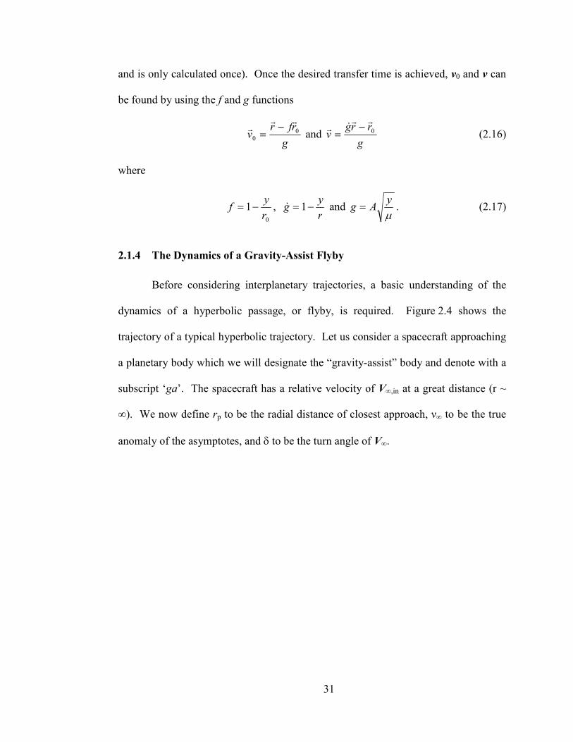
Before considering interplanetary trajectories, a basic understanding of the
dynamics of a hyperbolic passage, or flyby, is required. Figure 2.4 shows the
trajectory of a typical hyperbolic trajectory. Let us consider a spacecraft approaching
a planetary body which we will designate the “gravity-assist” body and denote with a
subscript ‘ga’. The spacecraft has a relative velocity of V∞,in at a great distance (r ~
∞). We now define rp to be the radial distance of closest approach, ν∞ to be the true
anomaly of the asymptotes, and δ to be the turn angle of V∞.
32
Figure 2.4. Geometry of a Hyperbolic Passage. Vga is th velocity vector of the gravity-assist body. The V∞ vector of the spacecraft has a true anomaly at infinity of ν∞. The point of closest approach is designated rp. The V∞ vector is bent by an the
turn angle, δ. Subscript ‘in’ represents conditions before the fly-by, ‘out’ subscripts are after the fly-by.
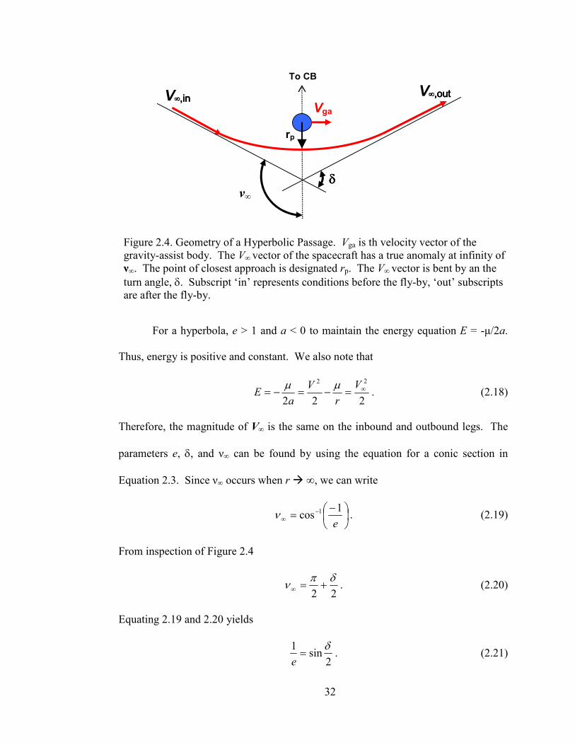
For a hyperbola, e > 1 and a < 0 to maintain the energy equation E = -µ/2a.
Thus, energy is positive and constant. We also note that
222
22∞=−=−=
V
r
V
aE
µµ. (2.18)
Therefore, the magnitude of V∞ is the same on the inbound and outbound legs. The
parameters e, δ, and ν∞ can be found by using the equation for a conic section in
Equation 2.3. Since ν∞ occurs when r ∞, we can write
−= −
∞e
1cos 1ν . (2.19)
From inspection of Figure 2.4
22
δπν +=∞ . (2.20)
Equating 2.19 and 2.20 yields
2
sin1 δ
=e
. (2.21)
ν∞
Vga
V∞,in∞,in∞,in∞,in V∞,out∞,out∞,out∞,out
To CB
δδδδ
rp
33
From the energy relation in Equation 2.18, the semimajor axis of the hyperbola is
given by a = -µ/V∞2. Substituting this into Equation 2.3 gives us an equation for the
eccentricity
µ
2
1∞+=
Vre
p. (2.22)
The amount of bending, or turn angle, gained by a flyby is governed by the mass of
the gravity-assist body, µ, the magnitude of V∞, and the closest approach, rp:
+=
∞
−2
1sin2Vrpµ
µδ . (2.23)
The discussion thus far has dealt with quantities in the inertial frame centered
on the gravity-assist body. However, the assist body has a velocity of its own in an
overall inertial frame centered on a central body. The hyperbolic excess velocity
with respect to the gravity-assist body, or the V∞ vector, is in fact defined as the
velocity of the spacecraft with respect to the central body, Vsc, minus the velocity of
the gravity-assist body, Vga:
gasc VVVrrr
−=∞ . (2.24)
This relationship is best described by the velocity triangle in Figure 2.5. If the
gravity-assist body is in a circular orbit, as is the assumed case for this dissertation,
then the angle between Vsc and Vga is the flight path angle, γ. The direction of the V∞
vector is defined by the angle α, which is the angle between V∞ and Vga and varies
from 0° (parallel) and 180° (anti-parallel). This is known as the “pump” angle
(Uphoff, 1976), as changing α changes the orbital energy directly.
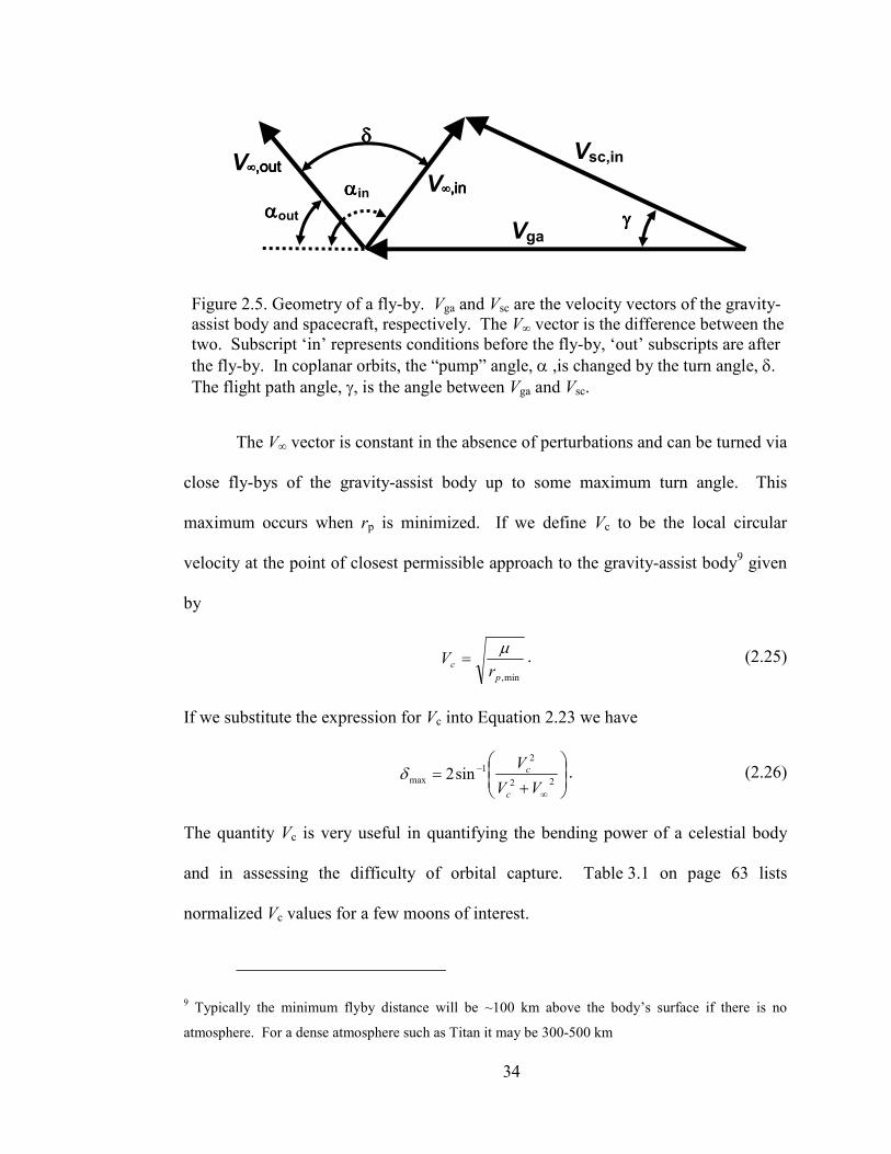
34
Figure 2.5. Geometry of a fly-by. Vga and Vsc are the velocity vectors of the gravity-assist body and spacecraft, respectively. The V∞ vector is the difference between the two. Subscript ‘in’ represents conditions before the fly-by, ‘out’ subscripts are after
the fly-by. In coplanar orbits, the “pump” angle, α ,is changed by the turn angle, δ.
The flight path angle, γ, is the angle between Vga and Vsc.
The V∞ vector is constant in the absence of perturbations and can be turned via
close fly-bys of the gravity-assist body up to some maximum turn angle. This
maximum occurs when rp is minimized. If we define Vc to be the local circular
velocity at the point of closest permissible approach to the gravity-assist body9 given
by
min,p
cr
Vµ
= . (2.25)
If we substitute the expression for Vc into Equation 2.23 we have
+=
∞
−22
21
max sin2VV
V
c
cδ . (2.26)
The quantity Vc is very useful in quantifying the bending power of a celestial body
and in assessing the difficulty of orbital capture. Table 3.1 on page 63 lists
normalized Vc values for a few moons of interest.
9 Typically the minimum flyby distance will be ~100 km above the body’s surface if there is no
atmosphere. For a dense atmosphere such as Titan it may be 300-500 km
ααααout
Vga
Vsc,in
V∞,in∞,in∞,in∞,in
V∞,out∞,out∞,out∞,out ααααin
γγγγ
δδδδ
35
The outgoing direction after a flyby can be controlled by fine tuning the
approach condition via small orbital maneuvers. This is known as B-plane targeting.
Typically these maneuvers only require a few m/s of ∆V or less. The new V∞ vector
also leads to a new Vsc vector that may be longer or shorter than prior to the flyby.
This means that the orbital parameters and energy with respect to the central body can
be modified to suit mission needs for a negligible cost in fuel. For this reason flybys
are often called gravity-assists. The boost gained by a gravity assist is given by
=∆ ∞2
sin2δ
VV fb. (2.27)
The realm of possible orbital parameters following a flyby can be plotted on a map
called a V∞ Sphere, as described in Section 3.3.
Orbital Capture. Many scientific missions end with an orbit about a target
planet or moon. This can be achieved by reducing energy during hyperbolic passage.
The simplest method of establishing a circular orbit with one decelerating impulse is
to adjust the approach parameters such that the distance of closest approach is equal
to the final orbit radius, rc. When this point is reached an orbital insertion maneuver
is performed to slow the spacecraft. The size of the maneuver is given by
cc rr
VVµµ
−+=∆ ∞
22 . (2.28)
This maneuver may be optimized when the final orbit radius is not critical.
To minimize ∆V, we take the derivative of Equation 2.28 with respect to rc and set it
equal to zero, noting that V∞ is constant
36
02
1
23
2
2
=+
+
−
=∂∆∂
∞c
c
c
c r
rV
r
r
V µ
µ
µ
. (2.29)
This indicates that the minimum ∆V occurs when
2
2
∞
=V
rc
µ (2.30)
and has the value
2
min∞=∆
VV . (2.31)
2.1.5 Patched Two-Body Trajectories
The patched two-body approximation is a method to simplify trajectory
calculations for spacecraft in a multiple body environment. The simplification is
achieved by dividing space into various parts by assigning each of the n bodies (e.g.
the Sun, planets, moons) its own sphere of influence. When the spacecraft is within
the sphere of influence of a smaller body, only the gravitational force between the
spacecraft and that smaller body is considered, otherwise the gravitational force
between the spacecraft and the larger body is used. This reduces an unsolvable n-
body problem to multiple solvable two-body problems, for which the solutions are the
well-known conic sections of the Keplerian orbits. This method gives a good
approximation of trajectories for interplanetary spacecraft missions.
Defining the sphere of influence (SOI) of the smaller body is not as simple as
calculating the location where its gravitational pull is stronger than that of the larger.
If this were the case, then the moon would fall 50% outside of the Earth’s SOI, which
is obviously not true. The correct definition of SOI, due to Laplace, involves
37
considering the spacecraft to be in orbit about one body and calculating the perturbing
force due to the other body. This allows us to determine the ratio of the disturbing
acceleration to the central body attraction. The resulting analysis yields the
approximate radius of the SOI
Rm
mrSOI
5/2
1
2
= , (2.32)
where R is the distance between the two bodies and m1 >> m2.
The SOI is both very large and extremely small, depending on your frame of
reverence. Relative to the size of m2 it is so large so as to consider it at infinity.
Relative to m1, it is essentially a point and of little consequence. Because it is so
large in the first case, the velocity relative to m2 exiting the SOI on an escape
hyperbola is considered to be the V∞ vector. This vector is then added to the smaller
body’s orbital velocity to obtain the spacecraft’s velocity with respect to the larger
body. This velocity, along with the position upon exiting the SOI, determines the
Keplerian orbit about m1 until the SOI of a smaller body is again entered.
As a simplification due to the smallness of the SOI in the larger reference
frame, the effects of a flyby can be considered to be instantaneous and occur exactly
at the location of the smaller body. This is called a zero sphere-of-influence method
of patched conics. This eliminates the need to calculate the actual location of the SOI
boundary crossing and convert to the new reference frame. We can also assume that
the B-plane targeting that controls the turn angle, δ, is negligible and occurs
automatically to meet the mission design’s needs. This method is used in the analysis
of V∞ leveraging in Chapter 3.
38
2.2 The Three-Body Problem
In this section the equations governing the PR3BP and planar Hill’s Problem
are set forth. Using consistent notation and quantities it is possible to show their
equivalences under specified assumptions. Writing the 3BP Jacobi integral in an
inertial coordinate system permits a derivation of Tisserand’s criterion and also
allows a relationship with 2BP orbital parameters and quantities, specifically V∞.
2.2.1 Planar Circular Restricted Three-Body Problem
The primary body, m1, and the secondary body, m2, are assumed to be in
circular orbits relative to each other and their center of mass, or barycenter, as
illustrated in Figure 2.6. They are separated by a distance R. The coordinate frame,
X-Y, rotates with constant angular velocity, ω, given by
3
21
R
µµω
+= , (2.33)
where µ1(or2) = Gm1(or2) and G is the gravitational constant. A massless third body, m3,
is located at
22 YXr += (2.34)
22
22
22
11
)(
)(
YRXr
YRXr
+−=
++= (2.35)
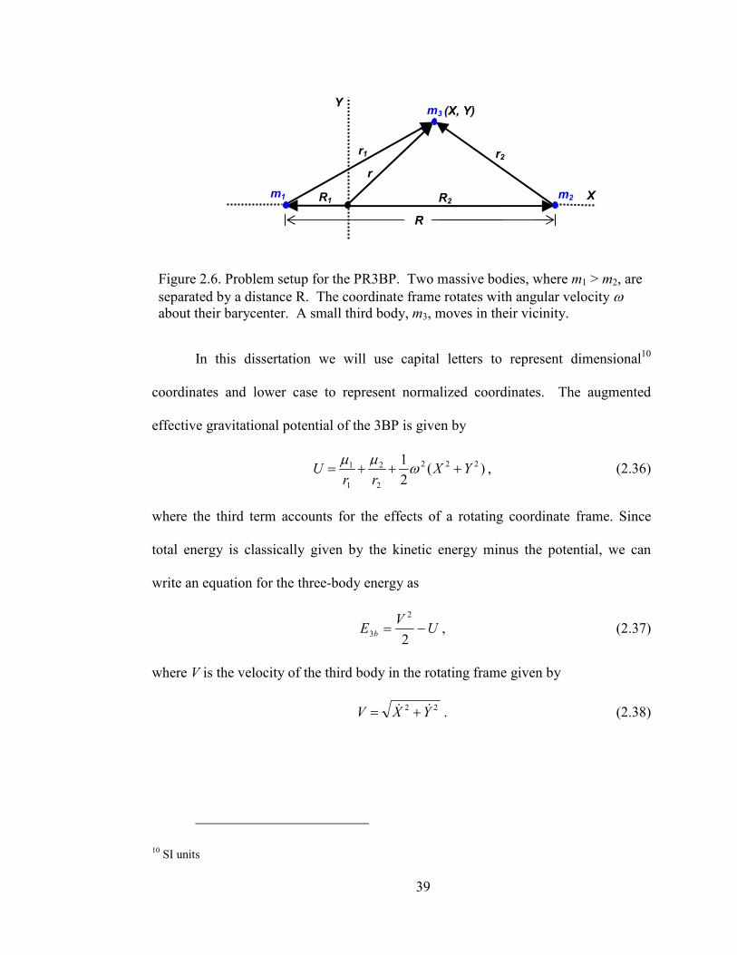
39
Figure 2.6. Problem setup for the PR3BP. Two massive bodies, where m1 > m2, are
separated by a distance R. The coordinate frame rotates with angular velocity ω about their barycenter. A small third body, m3, moves in their vicinity.
In this dissertation we will use capital letters to represent dimensional10
coordinates and lower case to represent normalized coordinates. The augmented
effective gravitational potential of the 3BP is given by
)(2
1 222
2
2
1
1 YXrr
U +++= ωµµ
, (2.36)
where the third term accounts for the effects of a rotating coordinate frame. Since
total energy is classically given by the kinetic energy minus the potential, we can
write an equation for the three-body energy as
UV
E b −=2
2
3 , (2.37)
where V is the velocity of the third body in the rotating frame given by
22 YXV && += . (2.38)
10 SI units
R1
R
r
r1
m2
r2
X
Y (X, Y) m3
m1 R2

40
2.2.2 Equations of Motion and Normalization
To scale the equations to any system, we introduce the mass parameter, µ,
given by
121
2 <<+
=µµ
µµ . (2.39)
We also set R = 1, m1 + m2 = 1, and ω = 1. This gives us R1 = µ, R2 = 1-µ, and the
orbital period P = 2π/ω = 2π. We can now write the equations of motion
3
2
3
1
3
2
3
1
)1(2
1)1(2
r
y
r
yyxy
r
x
r
xxyx
µµ
µµ
µµ
−−−+−=
+−−
+−−+=
&&&
&&&
(2.40)
where
22
2
22
1
)1(
)(
yxr
yxr
++−=
++=
µ
µ (2.41)
in normalized units. Last, the energy and Jacobi in nondimensional units can no be
written:
21
2222
3
1)(
2
1)(
2
1
rryxyxE
µµ−
−−+−+= && (2.42)
22
21
22
3
2)1(2yx
rryxJ && −−+
−++=
µµ (2.43)
where the subscript ‘3’ has been used to designate the non-dimensional form. For
orbits that are very close to m2, normalized energy, E3, is usually around -1.5 and J3 is
around 3. In order to readily convert between the dimensional and nondimensional
forms of the Jacobi, we can use the relation
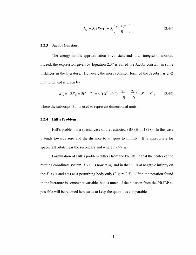
41
+==
RJRJJ b
213
2
33 )(µµ
ω . (2.44)
2.2.3 Jacobi Constant
The energy in this approximation is constant and is an integral of motion.
Indeed, the expression given by Equation 2.37 is called the Jacobi constant in some
instances in the literature. However, the most common form of the Jacobi has a -2
multiplier and is given by
22
2
2
1
12222
33
22)(22 YX
rrYXVUEJ bb
&& −−+++=−=−=µµ
ω , (2.45)
where the subscript ‘3b’ is used to represent dimensional units.
2.2.4 Hill’s Problem
Hill’s problem is a special case of the restricted 3BP (Hill, 1878). In this case
µ tends towards zero and the distance to m1 goes to infinity. It is appropriate for
spacecraft orbits near the secondary and where µ1 >> µ2.
Formulation of Hill’s problem differs from the PR3BP in that the center of the
rotating coordinate system, X’-Y’, is now at m2 and in that m1 is at negative infinity on
the X’ axis and acts as a perturbing body only (Figure 2.7). Often the notation found
in the literature is somewhat variable, but as much of the notation from the PR3BP as
possible will be retained here so as to keep the quantities comparable.
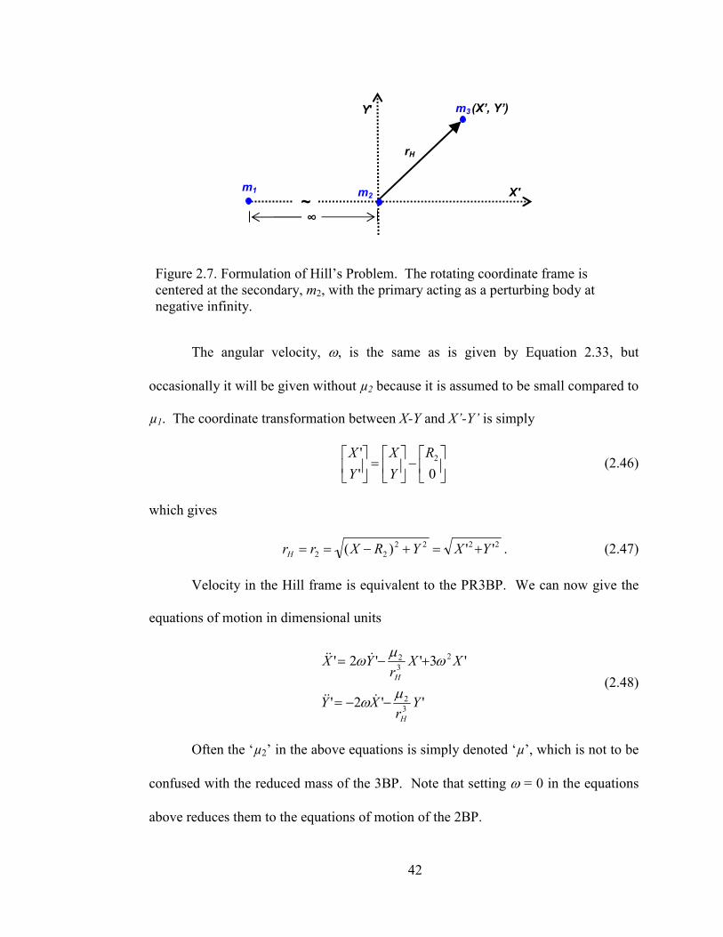
42
Figure 2.7. Formulation of Hill’s Problem. The rotating coordinate frame is centered at the secondary, m2, with the primary acting as a perturbing body at negative infinity.
The angular velocity, ω, is the same as is given by Equation 2.33, but
occasionally it will be given without µ2 because it is assumed to be small compared to
µ1. The coordinate transformation between X-Y and X’-Y’ is simply
−
=
0'
' 2R
Y
X
Y
X (2.46)
which gives
2222
22 '')( YXYRXrrH +=+−== . (2.47)
Velocity in the Hill frame is equivalent to the PR3BP. We can now give the
equations of motion in dimensional units
''2'
'3''2'
3
2
2
3
2
Yr
XY
XXr
YX
H
H
µω
ωµ
ω
−−=
+−=
&&&
&&&
(2.48)
Often the ‘µ2’ in the above equations is simply denoted ‘µ’, which is not to be
confused with the reduced mass of the 3BP. Note that setting ω = 0 in the equations
above reduces them to the equations of motion of the 2BP.
m3
X'
Y' (X’, Y’)
∞ ~
rH
m2 m1

43
The Jacobi integral in Hill’s problem is most commonly given by
222
2
, '2
3
2X
r
VJ
H
dH ωµ
−−= . (2.49)
Here, ‘H,d’ in the subscripts denotes the dimensional nature of the quantity. A lone
‘H’ will be used when referring to the normalized value. Note once again that setting
ω = 0 yields the equation for energy in the two-body problem.
Hill Normalization
Normalization in Hill’s problem is different from that of the PR3BP. Here the
length unit is not the separation between the primaries but is given by11
3
1
2
2
=
ωµ
l . (2.50)
The unit of time is given by τ = 1/ω. Using Equation 2.50 to normalize the distance
between m2 and m3, the realm of accuracy of Hill’s approximation is given by
3/1
1
32
+<
m
mmrH . (2.51)
These scale factors allow us to write the nondimensional equations of motion
3
3
''2'
'3'
'2'
H
H
r
yxy
xr
xyx
−−=
+−=
&&&
&&&
(2.52)
where x’, y’, and rH are normalized by dividing by the length unit in Equation 2.50.
The normalized Jacobi in Hill’s approximation is given by
11 l is approximately 1.5 times the distance to L1 or L2 and represents the radius of the Hill sphere.
44
22
'2
31
2x
r
VJ
H
H −−= . (2.53)
This most common form of the Jacobi, unlike the three-body formulation, is
similar to the two-body energy (kinetic minus potential) and does not contain the ‘-2’
multiplier. In his series on numerical exploration of the restricted problem, Hénon
(1969) uses the designation Γ as the integral of motion in Hill’s problem:
222 ''2
'3 yxr
xH
&& −−+=Γ , (2.54)
which is given here using our notation. When compared to Equation 2.53, it can be
seen that Γ = -2JH, which is analogous to the relationship between energy and Jacobi
in the 3BP.
We can readily convert between the dimensional and nondimensional forms of
the Jacobi by using the relationships
32
2
2
, )()( ωµω HHdH JlJJ == . (2.55)
2.2.5 The Jacobi Integral – PR3BP vs. Hill’s
Since velocity is equivalent in both reference frames, we start with Equation
2.45 plus 2 times Equation 2.49 to get
[ ]2222
1
1
2
22,3 '3)(2222 XYX
rrrJJ
H
dHb −+++−=+ ωµµµ
. (2.56)
Next we institute the Hill’s problem assumptions by presuming that the spacecraft is
close to the secondary and R2>>R1. These assumptions yield r1 ≅ R and rH = r2.
Substituting these relationships into Equation 2.56, we have
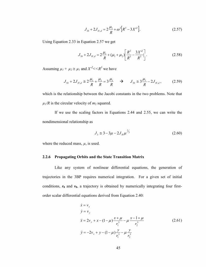
45
[ ]2221,3 '322 XR
RJJ dHb −+=+ ω
µ. (2.57)
Using Equation 2.33 in Equation 2.57 we get
−++=+
3
2
3
2
211
,3
'3)(22
R
X
R
R
RJJ dHb µµ
µ. (2.58)
Assuming µ1 + µ2 ≅ µ1 and X’2<<R
3 we have
RRR
JJ dHb111
,3 322µµµ
=+≅+ dHb JR
J ,1
3 23 −≅µ
, (2.59)
which is the relationship between the Jacobi constants in the two problems. Note that
µ1/R is the circular velocity of m2 squared.
If we use the scaling factors in Equations 2.44 and 2.55, we can write the
nondimensional relationship as
32
3 233 µµ HJJ −−≅ (2.60)
where the reduced mass, µ, is used.
2.2.6 Propagating Orbits and the State Transition Matrix
Like any system of nonlinear differential equations, the generation of
trajectories in the 3BP requires numerical integration. For a given set of initial
conditions, r0 and v0, a trajectory is obtained by numerically integrating four first-
order scalar differential equations derived from Equation 2.40:
3
2
3
1
3
2
3
1
)1(2
1)1(2
r
y
r
yyvy
r
x
r
xxvx
vy
vx
x
y
y
x
µµ
µµ
µµ
−−−+−=
+−−
+−−+=
=
=
&&
&&
&
&
(2.61)
46
where r1 and r2 are given by Equation 2.41.
From differential equation theory, any State Transition Matrix (STM or Ф)
defines, given the initial conditions, the solution to a set of linear differential
equations of the form
stAsr&r )(= (2.62)
where s is the state vector s = [x y x& y& ]T and A is a matrix that is a function of time.
The solution to this equation is
)(),()( 00 tstttsrr
Φ= (2.63)
where the STM, Ф, is the solution to the matrix differential equation
),()(),( 00 tttAtt Φ=Φ& . (2.64)
A Taylor series expansion of the 3BP equations of motion (Equation 2.40)
yields variational equations that can be integrated to find the STM. This linearization
determines and equation that governs how a small difference from a given solution
will behave. The solution to this variational equation is in the form of Equation 2.63,
but with s(t) replaced with δs(t).
While special cases occur where the STM can be found analytically, it is
typically found numerically using Equation 2.64, where the matrix A(t) is equal to
)(
)()(
ts
tstA r
&r
∂∂
= . (2.65)
In the PCR3BP, A(t) is equal to
Ω=
2
0)(
xxU
ItA , (2.66)
where
47
∂∂
∂∂
∂∂
∂∂
=
y
y
x
y
y
x
x
x
U xx &&
&&&&
and
−=Ω
01
10. (2.67)
2.2.7 Stability and the Monodromy Matrix
The STM from the initial time (t0) to the time after one period (t0 + P) is
referred to as the monodromy matrix. After being propagated for one full orbit, the
matrix contains information about every region that a spacecraft would pass through
along that orbit. The stability of a periodic orbit may be determined by analyzing the
eigenvalues of the orbit’s monodromy matrix. A random perturbation in the state of a
spacecraft on an unstable orbit will cause the particle’s state to exponentially diverge
from that of the original orbit over time.
The monodromy matrices of periodic orbits in the PCR3BP have four
eigenvalues: λ, 1/λ, 1, and 1. The fact that these eigenvalues occur in reciprocal pairs
is a consequence of the symplectic nature of the STM, while the pair of values equal
to one is a result of Jacobi integral of motion. The stability of an orbit is related to the
absolute value of the real component of each eigenvalues. If a value exists that is
greater than 1, this indicates that an orbit is unstable to perturbations along the
corresponding eigenvector. If the value is less than 1 then an orbit is considered to be
stable in that direction. In fact, the eigenvalues of Keplerian orbits are all equal to 1,
indicating that any perturbation neither grows nor decays.
The instability of periodic orbits indicates that both stable and unstable
manifolds exist, which lead to and leave from them, respectively. These manifolds
contain the set of all trajectories that a spacecraft may take if it is perturbed in the
48
direction of the orbit’s unstable eigenvector. They are invariant, meaning that a point
on the manifold will remain on the manifold as time evolves. Periodic orbits can be
useful as capture mechanisms as a spacecraft can arrive nearly ballistically on an
stable manifold, and then depart after a time on a stable manifold towards a lower
orbit.
2.2.8 The Single-Shooting Method
The search for periodic orbits in the 3BP is typically an iterative process. An
initial guess is propagated to some point where we check for some indicator of
periodicity (usually a form of symmetry). Knowledge of the dynamics of the system
allows for an educated update to the initial conditions and the process is repeated.
This continues until periodicity conditions are met and a solution is found. In this
section we lay out the equations for a form of differential correction known as the
single-shooting method.
The basic algorithm, described by Howell (1984), is modified here for the
planar case. It uses the symmetry about the x-axis in the CRTBP in order to search for
periodic orbits. This means that if a trajectory intersects the x-axis twice with a
velocity perpendicular to the x-axis, the trajectory will be periodic. In this method, a
point on the x-axis with initial conditions close to the desired orbit is integrated
forward in time until it returns to the x-axis. The requirement that the intersection
with the x-axis be perpendicular (i.e. x& = 0) imposes constraints that can be used to
modify the initial conditions. This process is repeated until a periodic orbit within the
desired tolerances is obtained. Howell found that if | x& | < 10-8, then the orbit can be
considered periodic.
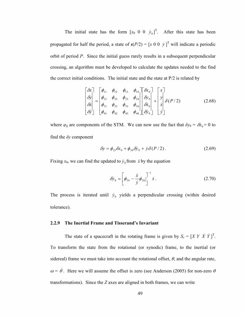
49
The initial state has the form [x0 0 0 0y& ]T. After this state has been
propagated for half the period, a state of s(P/2) = [x 0 0 y& ]T will indicate a periodic
orbit of period P. Since the initial guess rarely results in a subsequent perpendicular
crossing, an algorithm must be developed to calculate the updates needed to the find
the correct initial conditions. The initial state and the state at P/2 is related by
)2/(
0
0
0
0
44434241
34333231
24232221
14131211
P
y
x
y
x
y
x
y
x
y
x
y
x
δ
δδδδ
φφφφφφφφφφφφφφφφ
δδδδ
+
=
&
&
&
&
&
& (2.68)
where φij are components of the STM. We can now use the fact that δy0 = 0x&δ = 0 to
find the δy component
)2/(024021 Pyyxy δδφδφδ && ++= . (2.69)
Fixing x0, we can find the updated to 0y& from x& by the equation
xy
xy &
&
&&&
1
24340
−
−= φφδ . (2.70)
The process is iterated until 0y& yields a perpendicular crossing (within desired
tolerance).
2.2.9 The Inertial Frame and Tisserand’s Invariant
The state of a spacecraft in the rotating frame is given by Sr = [X Y X& Y& ]T.
To transform the state from the rotational (or synodic) frame, to the inertial (or
sidereal) frame we must take into account the rotational offset, θ, and the angular rate,
ω = θ& . Here we will assume the offset is zero (see Anderson (2005) for non-zero θ
transformations). Since the Z axes are aligned in both frames, we can write
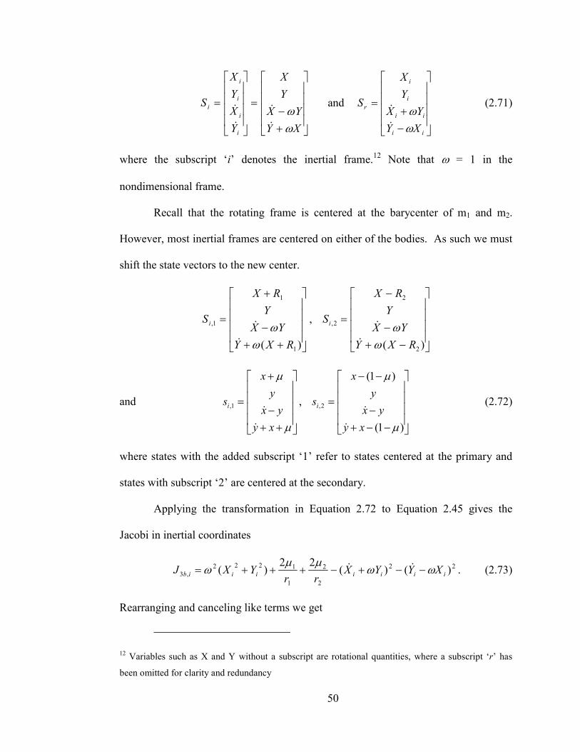
50
+
−=
=
XY
YX
Y
X
Y
X
Y
X
S
i
i
i
i
i
ωω
&
&
&
& and
−
+=
ii
ii
i
i
r
XY
YX
Y
X
S
ωω
&
& (2.71)
where the subscript ‘i’ denotes the inertial frame.12 Note that ω = 1 in the
nondimensional frame.
Recall that the rotating frame is centered at the barycenter of m1 and m2.
However, most inertial frames are centered on either of the bodies. As such we must
shift the state vectors to the new center.
++
−
+
=
)( 1
1
1,
RXY
YX
Y
RX
S i
ωω
&
&,
−+
−
−
=
)( 2
2
2,
RXY
YX
Y
RX
Si
ωω
&
&
and
++
−
+
=
µ
µ
xy
yx
y
x
si
&
&1, ,
−−+
−
−−
=
)1(
)1(
2,
µ
µ
xy
yx
y
x
si
&
& (2.72)
where states with the added subscript ‘1’ refer to states centered at the primary and
states with subscript ‘2’ are centered at the secondary.
Applying the transformation in Equation 2.72 to Equation 2.45 gives the
Jacobi in inertial coordinates
22
2
2
1
1222
,3 )()(22
)( iiiiiiib XYYXrr
YXJ ωωµµ
ω −−+−+++= && . (2.73)
Rearranging and canceling like terms we get
12 Variables such as X and Y without a subscript are rotational quantities, where a subscript ‘r’ has
been omitted for clarity and redundancy
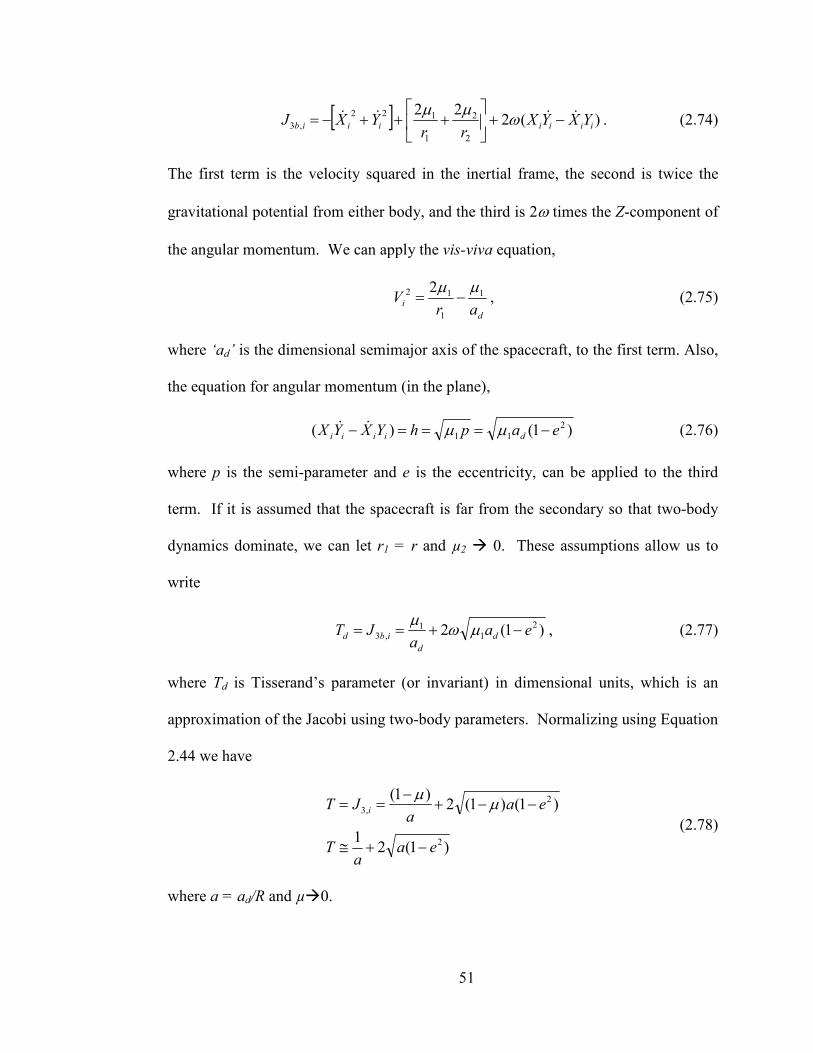
51
[ ] )(222
2
2
1
122
,3 iiiiiiib YXYXrr
YXJ &&&& −+
+++−= ω
µµ. (2.74)
The first term is the velocity squared in the inertial frame, the second is twice the
gravitational potential from either body, and the third is 2ω times the Z-component of
the angular momentum. We can apply the vis-viva equation,
d
iar
V 1
1
12 2 µµ−= , (2.75)
where ‘ad’ is the dimensional semimajor axis of the spacecraft, to the first term. Also,
the equation for angular momentum (in the plane),
)1()( 2
11 eaphYXYX diiii −===− µµ&& (2.76)
where p is the semi-parameter and e is the eccentricity, can be applied to the third
term. If it is assumed that the spacecraft is far from the secondary so that two-body
dynamics dominate, we can let r1 = r and µ2 0. These assumptions allow us to
write
)1(2 2
11
,3 eaa
JT d
d
ibd −+== µωµ
, (2.77)
where Td is Tisserand’s parameter (or invariant) in dimensional units, which is an
approximation of the Jacobi using two-body parameters. Normalizing using Equation
2.44 we have
)1(21
)1()1(2)1(
2
2
,3
eaa
T
eaa
JT i
−+≅
−−+−
== µµ
(2.78)
where a = ad/R and µ0.
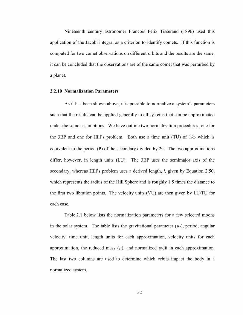
52
Nineteenth century astronomer Francois Felix Tisserand (1896) used this
application of the Jacobi integral as a criterion to identify comets. If this function is
computed for two comet observations on different orbits and the results are the same,
it can be concluded that the observations are of the same comet that was perturbed by
a planet.
2.2.10 Normalization Parameters
As it has been shown above, it is possible to normalize a system’s parameters
such that the results can be applied generally to all systems that can be approximated
under the same assumptions. We have outline two normalization procedures: one for
the 3BP and one for Hill’s problem. Both use a time unit (TU) of 1/ω which is
equivalent to the period (P) of the secondary divided by 2π. The two approximations
differ, however, in length units (LU). The 3BP uses the semimajor axis of the
secondary, whereas Hill’s problem uses a derived length, l, given by Equation 2.50,
which represents the radius of the Hill Sphere and is roughly 1.5 times the distance to
the first two libration points. The velocity units (VU) are then given by LU/TU for
each case.
Table 2.1 below lists the normalization parameters for a few selected moons
in the solar system. The table lists the gravitational parameter (µ2), period, angular
velocity, time unit, length units for each approximation, velocity units for each
approximation, the reduced mass (µ), and normalized radii in each approximation.
The last two columns are used to determine which orbits impact the body in a
normalized system.
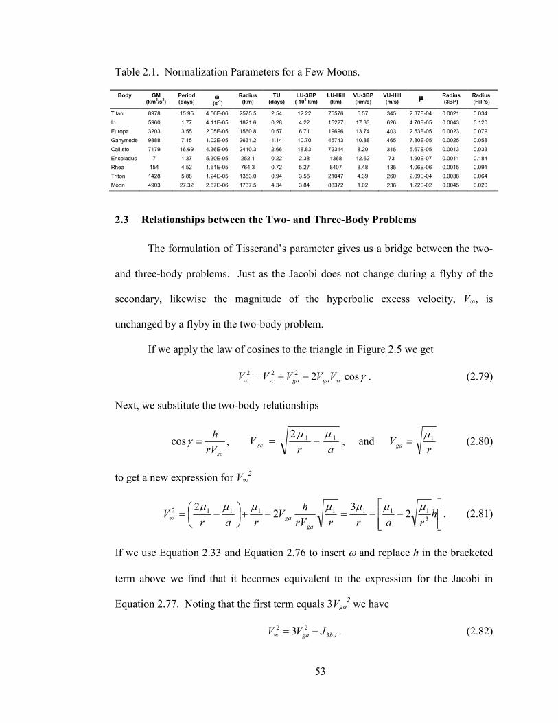
53
Table 2.1. Normalization Parameters for a Few Moons.
Body GM (km
3/s
2)
Period (days)
ωωωω (s
-1)
Radius (km)
TU (days)
LU-3BP ( 10
5 km)
LU-Hill (km)
VU-3BP (km/s)
VU-Hill (m/s)
µµµµ Radius (3BP)
Radius (Hill's)
Titan 8978 15.95 4.56E-06 2575.5 2.54 12.22 75576 5.57 345 2.37E-04 0.0021 0.034
Io 5960 1.77 4.11E-05 1821.6 0.28 4.22 15227 17.33 626 4.70E-05 0.0043 0.120
Europa 3203 3.55 2.05E-05 1560.8 0.57 6.71 19696 13.74 403 2.53E-05 0.0023 0.079
Ganymede 9888 7.15 1.02E-05 2631.2 1.14 10.70 45743 10.88 465 7.80E-05 0.0025 0.058
Callisto 7179 16.69 4.36E-06 2410.3 2.66 18.83 72314 8.20 315 5.67E-05 0.0013 0.033
Enceladus 7 1.37 5.30E-05 252.1 0.22 2.38 1368 12.62 73 1.90E-07 0.0011 0.184
Rhea 154 4.52 1.61E-05 764.3 0.72 5.27 8407 8.48 135 4.06E-06 0.0015 0.091
Triton 1428 5.88 1.24E-05 1353.0 0.94 3.55 21047 4.39 260 2.09E-04 0.0038 0.064
Moon 4903 27.32 2.67E-06 1737.5 4.34 3.84 88372 1.02 236 1.22E-02 0.0045 0.020
2.3 Relationships between the Two- and Three-Body Problems
The formulation of Tisserand’s parameter gives us a bridge between the two-
and three-body problems. Just as the Jacobi does not change during a flyby of the
secondary, likewise the magnitude of the hyperbolic excess velocity, V∞, is
unchanged by a flyby in the two-body problem.
If we apply the law of cosines to the triangle in Figure 2.5 we get
γcos2222
scgagasc VVVVV −+=∞ . (2.79)
Next, we substitute the two-body relationships
scrV
h=γcos ,
arV sc
112 µµ−= , and
rVga
1µ= (2.80)
to get a new expression for V∞2
−−=−+
−=∞ h
rarrrV
hV
rarV
ga
ga 3
11111112 23
22 µµµµµµµ
. (2.81)
If we use Equation 2.33 and Equation 2.76 to insert ω and replace h in the bracketed
term above we find that it becomes equivalent to the expression for the Jacobi in
Equation 2.77. Noting that the first term equals 3Vga2 we have
ibga JVV ,3
22 3 −=∞ . (2.82)
54
Now we have an expression for the relationship between the Jacobi and V∞. Vga is
constant for a circular orbit and yields a simple quadratic relationship. We can
normalize the expression by dividing each term by Vga2, noting that Vga
2 = (1-µ)(Rω)2
which is close to the term in Equation 2.44. Now we have
ii JJv ,3,3
2 31
13 −≅
−−=∞ µ
, (2.83)
where the lower-case v denotes the normalized quantity. Recall that µ<<1. Solving
Equations 2.82 and 2.83 for J we have
22
,3 3 ∞−= VVJ gaib and )3)(1( 2
,3 ∞−−= vJ i µ . (2.84)
V∞ and Hill’s Problem. Having derived the relationships between the PR3BP
and Hill’s Problem (Eqs. 2.59 and 2.60), we can now write the equivalence between
V∞ and JH:
dHJV ,
2 2=∞ and HJvµ
µ−
=∞1
23/2
2 ,13 (2.85)
and solving for J:
2
2
,∞=
VJ dH and 2
3/22
1∞
−= vJ H µ
µ. (2.86)
The relationships in Equations 2.84 and 2.86 indicate that V∞ is positive when
J3 goes below 3 or when JH is positive. These orbits are hyperbolic in the two-body
formulation but are bound to the “vicinity” when third body effects are taken into
account.
13 Equation 2.54 yields the relationship Γ−
−=∞ µ
µ1
3/22v .
55
3 V∞ Leveraging
In this chapter we start by introducing the concept of V∞ leveraging. We then
go on to describe the V∞ Sphere and the V∞ Plane, which serve as a map for the range
of all possible orbits accessible via leveraging maneuvers and fly-bys. In the next
section we mathematically describe V∞ leveraging maneuvers and present a new
analysis method using a Lambert’s Solver. From this, we plot contours of leveraging
maneuver efficiencies and present a method using only the most efficient V∞
leveraging maneuvers, fly-bys, and powered fly-bys14 to calculate the theoretical
minimum ∆V required to reduce V∞ to zero given an infinite flight time. Then we
explore the domain of finite tour sequences and compare the results to the theoretical
minimum. As is often the case in trajectory design, a trade must be made between
performance (minimizing ∆V) and time-of-flight (TOF).
In order to create the data to characterize this trade space, a Monte-Carlo type
simulation was set up to generate random sequences of resonances15 (not restricted to
integer resonances) along with associated fly-bys and V∞ leveraging maneuvers.
Pathway sequences are created in the simulation by following a predetermined rule or
14 A tangential ∆V maneuver performed at periapsis of the fly-by. Powered fly-bys become more
efficient than leveraging maneuvers for small values of V∞
15 This is similar to “resonance hopping” tours found in the literature

56
set of rules. For example, a sequence may require that only integer resonances be
used and that non-tangential leveraging is not allowed. Each rule can be treated like a
heuristic where some trade between reduced fuel usage and increased flight time is
being made. Intuitively, there is a general trend towards decreasing ∆V by increasing
TOF. However, some pathway rules are not as effective as others in trading ∆V for
time and lead to contradictions to this trend.
Total ∆V is plotted versus TOF to create a Pareto front and to reveal the trends
that prove to be most efficient for V∞ leveraging sequencing. The derived heuristics
would be valuable to mission designers for both quick-look evaluations and in finding
a globally optimized solution given a set of mission parameters.
3.1 Introduction
V∞ leveraging is the use of a deep-space maneuver to modify the V∞ of the
spacecraft upon reencounter. These maneuvers are typically used in conjunction with
gravity-assists in order to change the spacecraft's energy and reduce the total ∆V for a
mission. The first example of such a maneuver was introduced by Hollenbeck (1975)
in the form of the ∆V-EGA (Delta-V Earth-Gravity-Assist). In this maneuver a
spacecraft is launched on a nearly resonant orbit with Earth, usually 2:1. A small
deep-space maneuver (~0.5 km/s) is then performed at aphelion to lower the
perihelion and reencounter Earth non-tangentially with a V∞ greater than that at
launch. As shown in Figure 3.1a, this fly-by can occur before or after the new
perihelion. In this manner the Earth can be used as a gravity-assist body to bend the
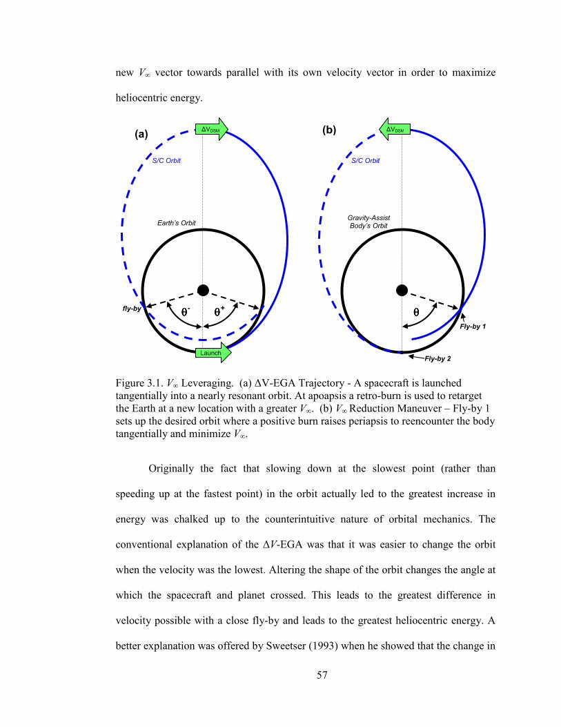
57
new V∞ vector towards parallel with its own velocity vector in order to maximize
heliocentric energy.
Figure 3.1. V∞ Leveraging. (a) ∆V-EGA Trajectory - A spacecraft is launched tangentially into a nearly resonant orbit. At apoapsis a retro-burn is used to retarget the Earth at a new location with a greater V∞. (b) V∞ Reduction Maneuver – Fly-by 1 sets up the desired orbit where a positive burn raises periapsis to reencounter the body tangentially and minimize V∞.
Originally the fact that slowing down at the slowest point (rather than
speeding up at the fastest point) in the orbit actually led to the greatest increase in
energy was chalked up to the counterintuitive nature of orbital mechanics. The
conventional explanation of the ∆V-EGA was that it was easier to change the orbit
when the velocity was the lowest. Altering the shape of the orbit changes the angle at
which the spacecraft and planet crossed. This leads to the greatest difference in
velocity possible with a close fly-by and leads to the greatest heliocentric energy. A
better explanation was offered by Sweetser (1993) when he showed that the change in
Gravity-Assist Body’s Orbit
S/C Orbit
θθθθ
∆VDSM
Fly-by 2
Fly-by 1
(b)
fly-by
Earth’s Orbit
S/C Orbit
θθθθ- θθθθ+
∆VDSM
Launch
(a)
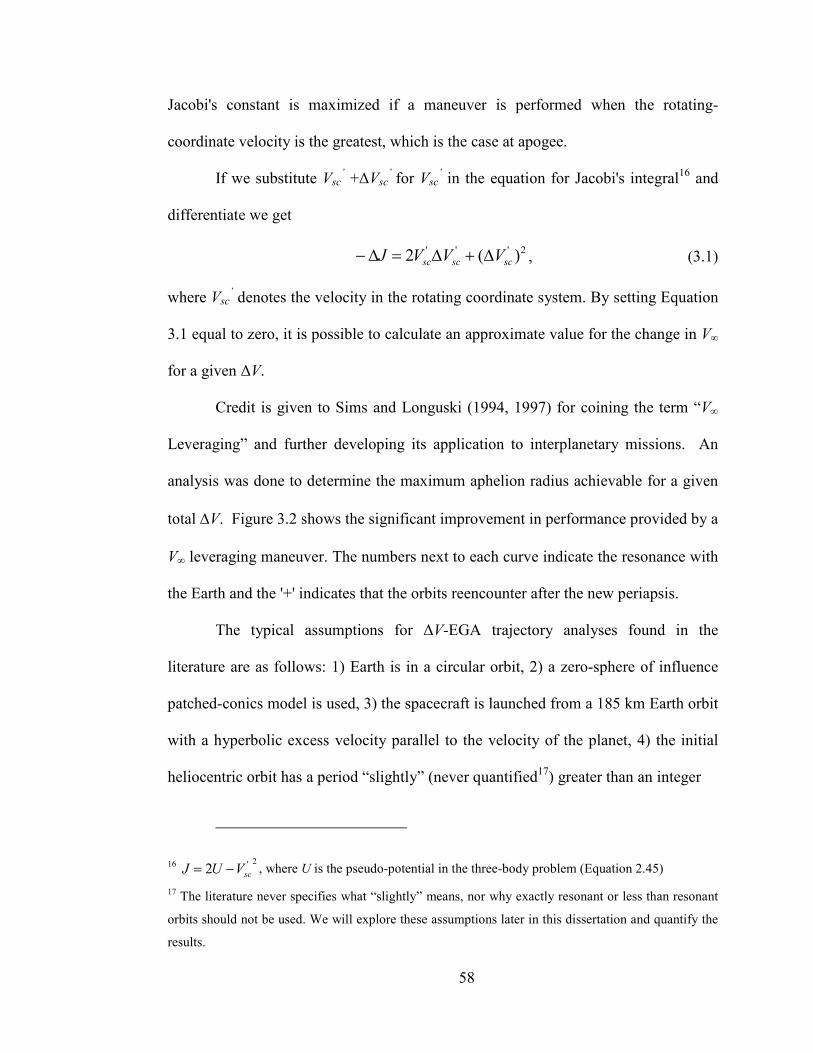
58
Jacobi's constant is maximized if a maneuver is performed when the rotating-
coordinate velocity is the greatest, which is the case at apogee.
If we substitute Vsc’ +∆Vsc
’ for Vsc
’ in the equation for Jacobi's integral16 and
differentiate we get
2''' )(2 scscsc VVVJ ∆+∆=∆− , (3.1)
where Vsc’ denotes the velocity in the rotating coordinate system. By setting Equation
3.1 equal to zero, it is possible to calculate an approximate value for the change in V∞
for a given ∆V.
Credit is given to Sims and Longuski (1994, 1997) for coining the term “V∞
Leveraging” and further developing its application to interplanetary missions. An
analysis was done to determine the maximum aphelion radius achievable for a given
total ∆V. Figure 3.2 shows the significant improvement in performance provided by a
V∞ leveraging maneuver. The numbers next to each curve indicate the resonance with
the Earth and the '+' indicates that the orbits reencounter after the new periapsis.
The typical assumptions for ∆V-EGA trajectory analyses found in the
literature are as follows: 1) Earth is in a circular orbit, 2) a zero-sphere of influence
patched-conics model is used, 3) the spacecraft is launched from a 185 km Earth orbit
with a hyperbolic excess velocity parallel to the velocity of the planet, 4) the initial
heliocentric orbit has a period “slightly” (never quantified17) greater than an integer
16 2'2 scVUJ −= , where U is the pseudo-potential in the three-body problem (Equation 2.45)
17 The literature never specifies what “slightly” means, nor why exactly resonant or less than resonant
orbits should not be used. We will explore these assumptions later in this dissertation and quantify the
results.
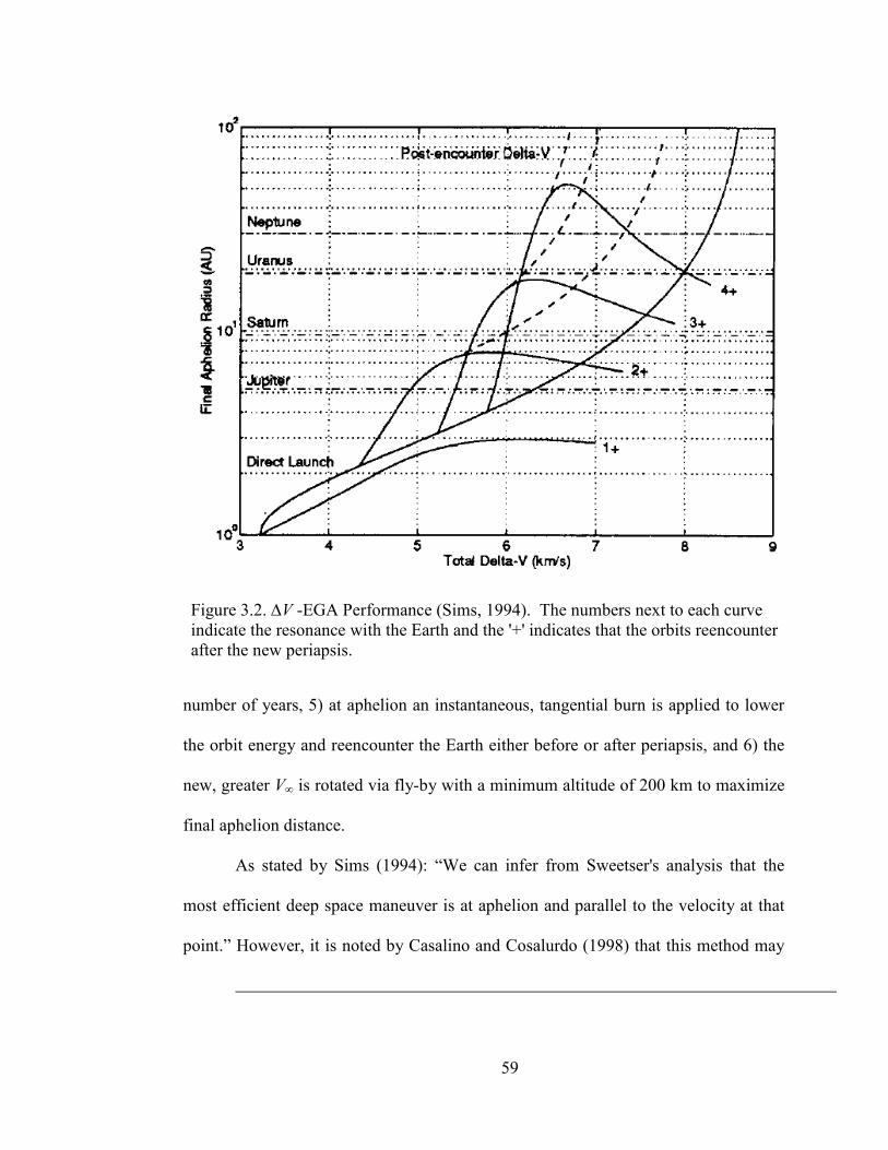
59
Figure 3.2. ∆V -EGA Performance (Sims, 1994). The numbers next to each curve indicate the resonance with the Earth and the '+' indicates that the orbits reencounter after the new periapsis.
number of years, 5) at aphelion an instantaneous, tangential burn is applied to lower
the orbit energy and reencounter the Earth either before or after periapsis, and 6) the
new, greater V∞ is rotated via fly-by with a minimum altitude of 200 km to maximize
final aphelion distance.
As stated by Sims (1994): “We can infer from Sweetser's analysis that the
most efficient deep space maneuver is at aphelion and parallel to the velocity at that
point.” However, it is noted by Casalino and Cosalurdo (1998) that this method may
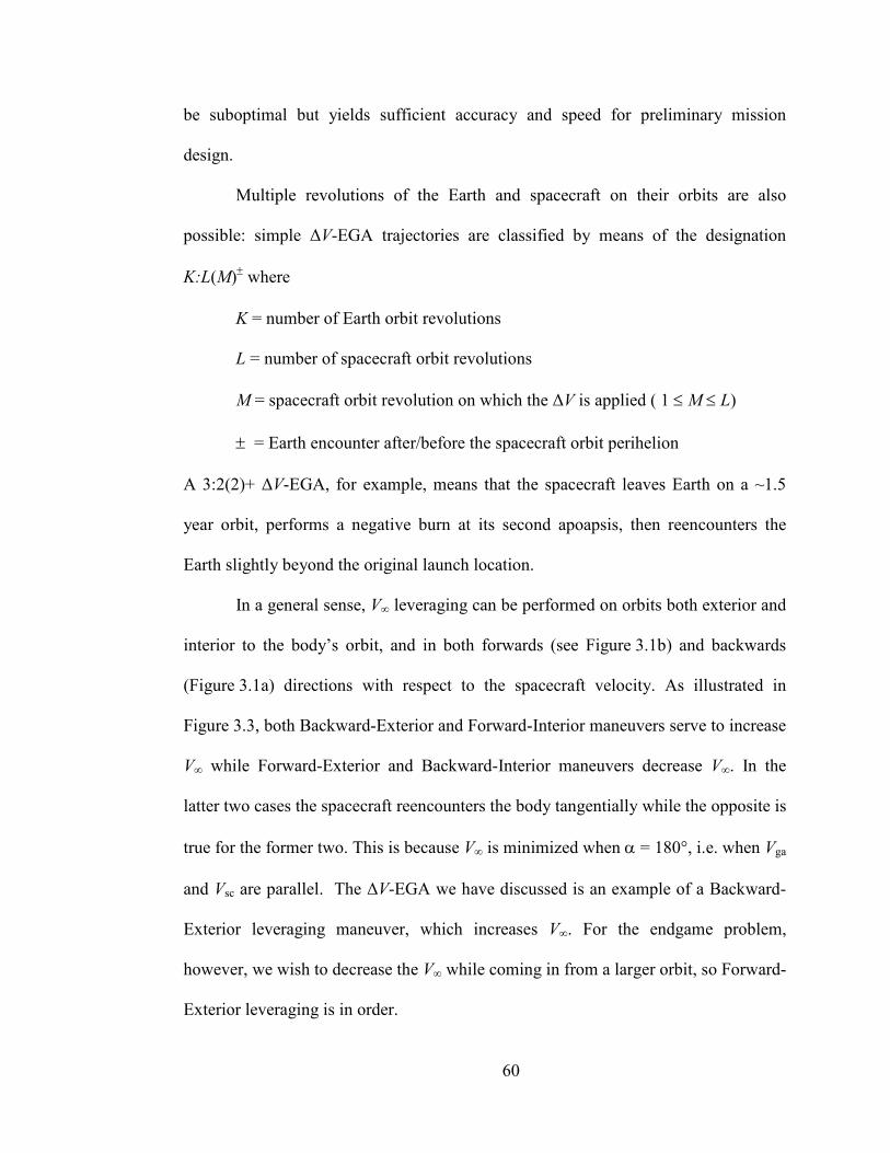
60
be suboptimal but yields sufficient accuracy and speed for preliminary mission
design.
Multiple revolutions of the Earth and spacecraft on their orbits are also
possible: simple ∆V-EGA trajectories are classified by means of the designation
K:L(M)± where
K = number of Earth orbit revolutions
L = number of spacecraft orbit revolutions
M = spacecraft orbit revolution on which the ∆V is applied ( 1 ≤ M ≤ L)
± = Earth encounter after/before the spacecraft orbit perihelion
A 3:2(2)+ ∆V-EGA, for example, means that the spacecraft leaves Earth on a ~1.5
year orbit, performs a negative burn at its second apoapsis, then reencounters the
Earth slightly beyond the original launch location.
In a general sense, V∞ leveraging can be performed on orbits both exterior and
interior to the body’s orbit, and in both forwards (see Figure 3.1b) and backwards
(Figure 3.1a) directions with respect to the spacecraft velocity. As illustrated in
Figure 3.3, both Backward-Exterior and Forward-Interior maneuvers serve to increase
V∞ while Forward-Exterior and Backward-Interior maneuvers decrease V∞. In the
latter two cases the spacecraft reencounters the body tangentially while the opposite is
true for the former two. This is because V∞ is minimized when α = 180°, i.e. when Vga
and Vsc are parallel. The ∆V-EGA we have discussed is an example of a Backward-
Exterior leveraging maneuver, which increases V∞. For the endgame problem,
however, we wish to decrease the V∞ while coming in from a larger orbit, so Forward-
Exterior leveraging is in order.
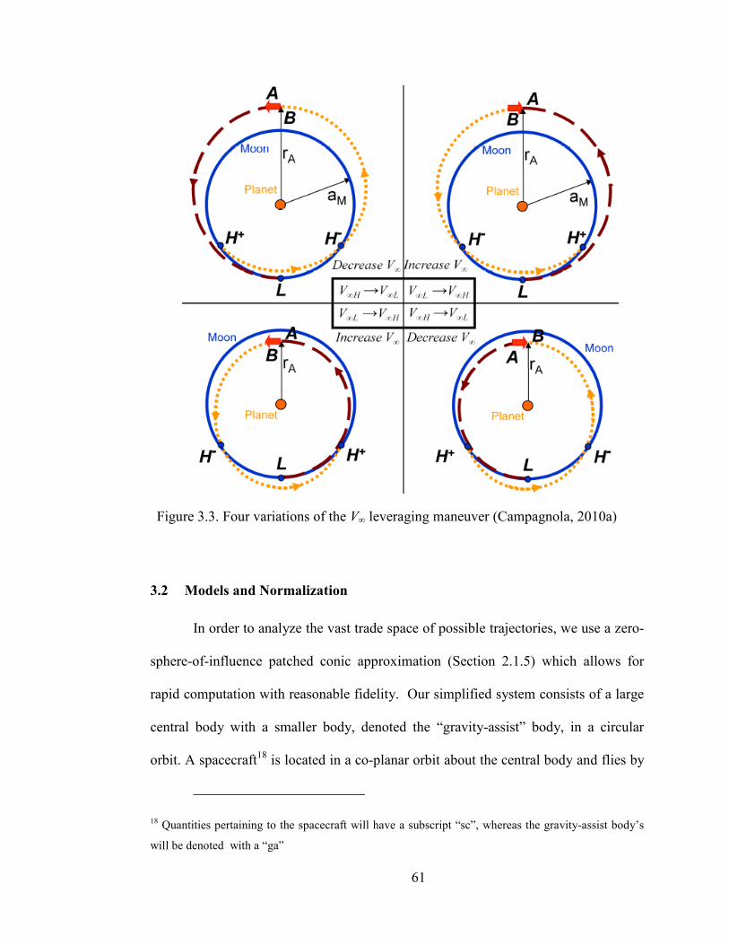
61
Figure 3.3. Four variations of the V∞ leveraging maneuver (Campagnola, 2010a)
3.2 Models and Normalization
In order to analyze the vast trade space of possible trajectories, we use a zero-
sphere-of-influence patched conic approximation (Section 2.1.5) which allows for
rapid computation with reasonable fidelity. Our simplified system consists of a large
central body with a smaller body, denoted the “gravity-assist” body, in a circular
orbit. A spacecraft18 is located in a co-planar orbit about the central body and flies by
18 Quantities pertaining to the spacecraft will have a subscript “sc”, whereas the gravity-assist body’s
will be denoted with a “ga”
62
the gravity-assist body with the ultimate goal of gravitational capture at that body.
The spacecraft is governed by the two-body equations of motion and is perturbed
instantaneously during encounters with the gravity-assist body.
The hyperbolic excess velocity with respect to the gravity-assist body, or the
V∞ vector, is constant in the absence of perturbations and can be turned via close fly-
bys of the gravity-assist body up to the maximum turn angle, given by Equation 2.26.
The direction of the V∞ vector is defined by the angle α, which is the angle between
V∞ and Vga and varies from 0° (parallel) and 180° (anti-parallel) (See Figure 2.5).
Because the V∞ vectors before and after have the same length, the locus of all possible
V∞’s after fly-by lie on a sphere centered at the head of Vga.
Changing α via fly-by, coined “orbit pumping” by Uphoff et. al.(1976),
changes the orbital energy and period about the central body. Post-fly-by orbital
parameters are controlled through suitable selection of encounter conditions such that
δmax given in Equation 2.26 yields a new V∞,out vector that results in the desired
outgoing velocity and period. The contours of all possible post-fly-by orbit
parameters (inclination, period, resonance, periapsis, etc.) can be mapped onto the
surface of a sphere (or V∞ globe) as an aid to mission design (Strange et al., 2007).
Sequences of same-body transfers can be mapped across the surface of this globe in
steps equal to or less than δmax.
The normalized units described by Section 2.2.10 are used throughout this
dissertation so that the results can be applied to any system with the proper scaling.
Recall that normalization is achieved by dividing length, velocity, and time by the
semimajor axis (a), circular velocity (Vga), and period (P) of the gravity-assist body,
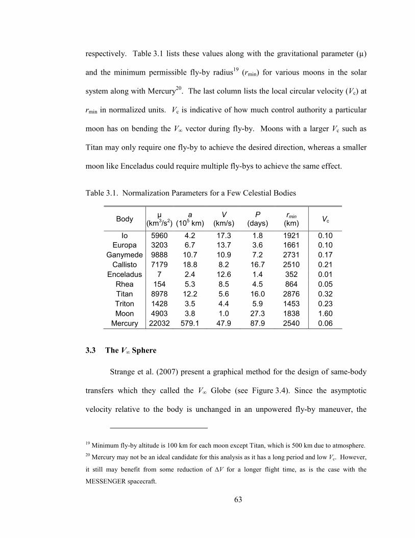
63
respectively. Table 3.1 lists these values along with the gravitational parameter (µ)
and the minimum permissible fly-by radius19 (rmin) for various moons in the solar
system along with Mercury20. The last column lists the local circular velocity (Vc) at
rmin in normalized units. Vc is indicative of how much control authority a particular
moon has on bending the V∞ vector during fly-by. Moons with a larger Vc such as
Titan may only require one fly-by to achieve the desired direction, whereas a smaller
moon like Enceladus could require multiple fly-bys to achieve the same effect.
Table 3.1. Normalization Parameters for a Few Celestial Bodies
Body µ
(km3/s2) a
(105 km) V
(km/s) P
(days) rmin
(km) Vc
Io 5960 4.2 17.3 1.8 1921 0.10
Europa 3203 6.7 13.7 3.6 1661 0.10
Ganymede 9888 10.7 10.9 7.2 2731 0.17
Callisto 7179 18.8 8.2 16.7 2510 0.21
Enceladus 7 2.4 12.6 1.4 352 0.01
Rhea 154 5.3 8.5 4.5 864 0.05
Titan 8978 12.2 5.6 16.0 2876 0.32
Triton 1428 3.5 4.4 5.9 1453 0.23
Moon 4903 3.8 1.0 27.3 1838 1.60
Mercury 22032 579.1 47.9 87.9 2540 0.06
3.3 The V∞ Sphere
Strange et al. (2007) present a graphical method for the design of same-body
transfers which they called the V∞ Globe (see Figure 3.4). Since the asymptotic
velocity relative to the body is unchanged in an unpowered fly-by maneuver, the
19 Minimum fly-by altitude is 100 km for each moon except Titan, which is 500 km due to atmosphere.
20 Mercury may not be an ideal candidate for this analysis as it has a long period and low Vc. However,
it still may benefit from some reduction of ∆V for a longer flight time, as is the case with the
MESSENGER spacecraft.
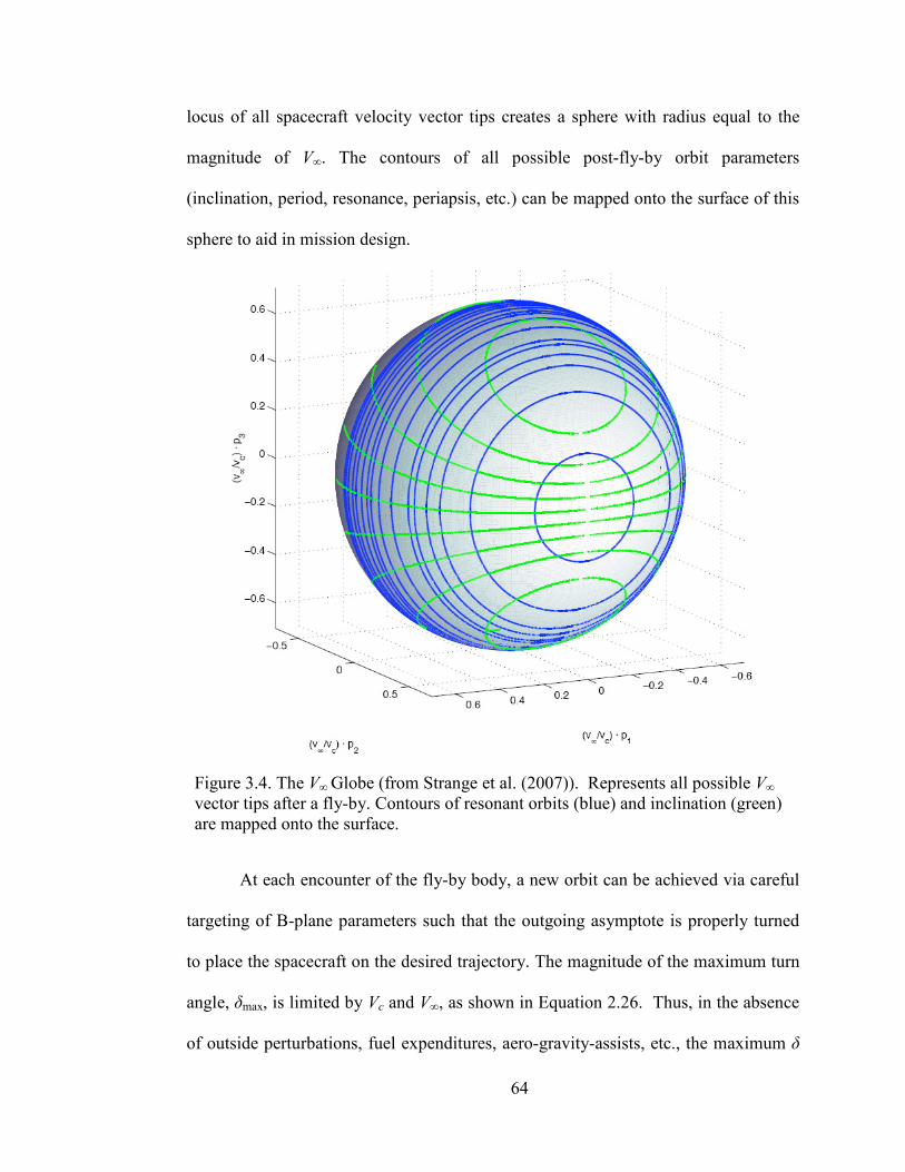
64
locus of all spacecraft velocity vector tips creates a sphere with radius equal to the
magnitude of V∞. The contours of all possible post-fly-by orbit parameters
(inclination, period, resonance, periapsis, etc.) can be mapped onto the surface of this
sphere to aid in mission design.
Figure 3.4. The V∞ Globe (from Strange et al. (2007)). Represents all possible V∞ vector tips after a fly-by. Contours of resonant orbits (blue) and inclination (green) are mapped onto the surface.
At each encounter of the fly-by body, a new orbit can be achieved via careful
targeting of B-plane parameters such that the outgoing asymptote is properly turned
to place the spacecraft on the desired trajectory. The magnitude of the maximum turn
angle, δmax, is limited by Vc and V∞, as shown in Equation 2.26. Thus, in the absence
of outside perturbations, fuel expenditures, aero-gravity-assists, etc., the maximum δ
65
represents the angular “step” size21 across the surface of the V∞ Globe. The
individual orbits of a tour can be plotted along the surface of the globe as points
separated by less than the maximum turn angle.
The entire surface of the V∞ Globe is not accessible in practice, even if an
unlimited number of fly-bys are used. For example, there is a region which separates
prograde and retrograde orbits that impacts the central body, making it practically
impossible to reverse an orbit from retrograde to prograde using a gravity-assist. If V∞
is great enough, there is a large area on the globe where the orbit becomes hyperbolic
with respect to the central body and escapes the system.
3.3.1 Accessible Regions
Using the law of cosines for the triangle made up of the velocity vectors in
Figure 2.5, we get
αcos2222
gagasc VVVVV ∞∞ ++= . (3.2)
If we utilize the normalized form of the vis-viva equation to solve for Vga in terms of
Vsc and asc we can substitute and rearrange Equation 3.2 to get an equation for the
inverse semimajor axis in terms of V∞ and α:
αcos21 21
∞∞− −−= VVasc .22 (3.3)
With V∞ fixed and α limited to 0°-180°, we now have bounds on asc:
∞∞−
∞∞ −−≤≤+− VVaVV sc 2121 212. (3.4)
21 As an example, at the end of its prime mission, the Cassini probe had a V∞ of 5.8 km/s and a
maximum δ of 8°.
22 For a more detailed derivation see Strange et al. (2007)
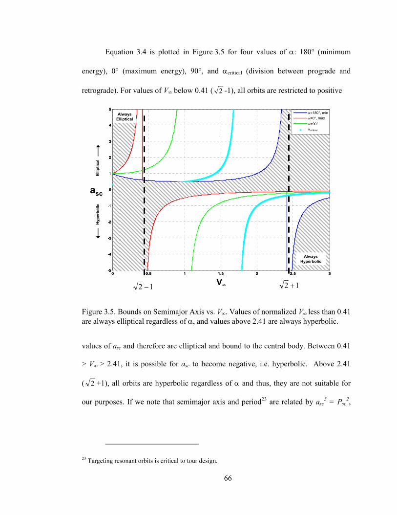
66
Equation 3.4 is plotted in Figure 3.5 for four values of α: 180° (minimum
energy), 0° (maximum energy), 90°, and αcritical (division between prograde and
retrograde). For values of V∞ below 0.41 ( 2 -1), all orbits are restricted to positive
0 0.5 1 1.5 2 2.5 3-5
-4
-3
-2
-1
0
1
2
3
4
5
Vinf
/ Vga
asc /
rga
min,a=180
max,a=0
a=90
a=ac
asc
V∞
α=180°, min
α=0°, max
α=90°
αcritical
0 0.5 1 1.5 2 2.5 3-5
-4
-3
-2
-1
0
1
2
3
4
5
Vinf
/ Vga
asc /
rga
min,a=180
max,a=0
a=90
a=ac
asc
V∞
0 0.5 1 1.5 2 2.5 3-5
-4
-3
-2
-1
0
1
2
3
4
5
Vinf
/ Vga
asc /
rga
min,a=180
max,a=0
a=90
a=ac
0 0.5 1 1.5 2 2.5 3-5
-4
-3
-2
-1
0
1
2
3
4
5
Vinf
/ Vga
asc /
rga
min,a=180
max,a=0
a=90
a=ac
asc
V∞
α=180°, min
α=0°, max
α=90°
αcritical
Always
Elliptical
Always
Hyperbolic
Hyp
erb
oli
cE
llip
tical
Figure 3.5. Bounds on Semimajor Axis vs. V∞. Values of normalized V∞ less than 0.41
are always elliptical regardless of α, and values above 2.41 are always hyperbolic.
values of asc and therefore are elliptical and bound to the central body. Between 0.41
> V∞ > 2.41, it is possible for asc to become negative, i.e. hyperbolic. Above 2.41
( 2 +1), all orbits are hyperbolic regardless of α and thus, they are not suitable for
our purposes. If we note that semimajor axis and period23 are related by asc3 = Psc
2,
23 Targeting resonant orbits is critical to tour design.
12 − 12 +
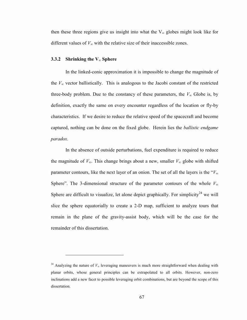
67
then these three regions give us insight into what the V∞ globes might look like for
different values of V∞ with the relative size of their inaccessible zones.
3.3.2 Shrinking the V∞ Sphere
In the linked-conic approximation it is impossible to change the magnitude of
the V∞ vector ballistically. This is analogous to the Jacobi constant of the restricted
three-body problem. Due to the constancy of these parameters, the V∞ Globe is, by
definition, exactly the same on every encounter regardless of the location or fly-by
characteristics. If we desire to reduce the relative speed of the spacecraft and become
captured, nothing can be done on the fixed globe. Herein lies the ballistic endgame
paradox.
In the absence of outside perturbations, fuel expenditure is required to reduce
the magnitude of V∞. This change brings about a new, smaller V∞ globe with shifted
parameter contours, like the next layer of an onion. The set of all the layers is the “V∞
Sphere”. The 3-dimensional structure of the parameter contours of the whole V∞
Sphere are difficult to visualize, let alone depict graphically. For simplicity24 we will
slice the sphere equatorially to create a 2-D map, sufficient to analyze tours that
remain in the plane of the gravity-assist body, which will be the case for the
remainder of this dissertation.
24 Analyzing the nature of V∞ leveraging maneuvers is much more straightforward when dealing with
planar orbits, whose general principles can be extrapolated to all orbits. However, non-zero
inclinations add a new facet to possible leveraging orbit combinations, but are beyond the scope of this
dissertation.
68
A planar slice of the V∞ Sphere, shown in Figure 3.6, depicts all the V∞ vector
tips of orbits lying in the plane of the gravity-assist body. The polar angle is the pump
angle (α), and the radial magnitude is V∞. The V∞ magnitudes, periapses (rp), and
apoapses (ra) are in normalized units. Orbits to the left of the green line are retrograde
Figure 3.6. The V∞ Plane. Represents all orbits possible after a planar flyby. Unpowered flybys may change α but will remain on concentric rings. The blue lines show contours of periapsis points while the magenta ones show apoapsis points. The green solid line separates prograde and retrograde orbits and the red dashed line encompasses the elliptical orbits.
with the dotted area around the line indicating orbits that would impact a typical
central body (Rcb/aga = 0.05). The red dotted line separates the elliptical orbit region
from the hyperbolic.
0.5
1
1.5
2
2.5
30
210
60
240
90
270
120
300
150
330
180 0
0.0
5
0.05
0.05
0.0
5
0. 1
0.1
0.1
0. 1
0.2
0.20
.2
0.2
0.2
0.4
0.4
0.4
0.4
0.4
0.6
0.6
0.6
0.6
0.6
0.7
0.7
0.7
0.7
0.7
0.8
0.8
0.8
0.80.8
0.9
0.90.9
0.9
0.9
1.05
1.05
1.05
1.1
1.1
1.1
1.2
1.2
1.2
1.5
1.5
1.5
1.5
2
2
2
2
4
4
44
4
7
7
77
7
20
20
20
20
20
Vinf=2.41
rp
ra
αααα
V∞
1 1.5
HYPERBOLIC
ELLIPTICAL
Prograde Retrograde
2
69
A spacecraft is constrained to a concentric ring in the absence of a ∆V
maneuver. It can move along the ring in steps of δmax or less for free (i.e. no fuel
required) during fly-bys. Each fly-by would of necessity target a resonant orbit
(contours not depicted here for clarity) in order to return in a finite amount of time.
∆Vs place the spacecraft on a smaller ring which can then be traversed in steps of the
new δmax. An endgame tour could be represented by points creating a zigzagging path
towards the center of the map, at which point V∞ would equal zero and the spacecraft
would be at the limit of gravitational capture. The object now is to find the path that
requires the minimum total ∆V.
The same planar map in a Cartesian projection is shown in Figure 3.7. In this
projection the spacecraft can move left and right (changing α) on horizontal lines for
free, or expend fuel in order to move lower (lowering V∞). Prograde, elliptical orbits
are those found below the green and red lines, respectively. It can be seen why
retrograde orbits are not used in tours as they cannot reach V∞ = 0 without becoming
prograde first, which is prohibitively expensive, fuel-wise. In addition to the apses,
contours for eccentricity and resonance (Psc/Pga) given by
( ) 2/32 cos21−
∞∞ −−== αVVRP
P
ga
sc , (3.5)
are plotted on this map.
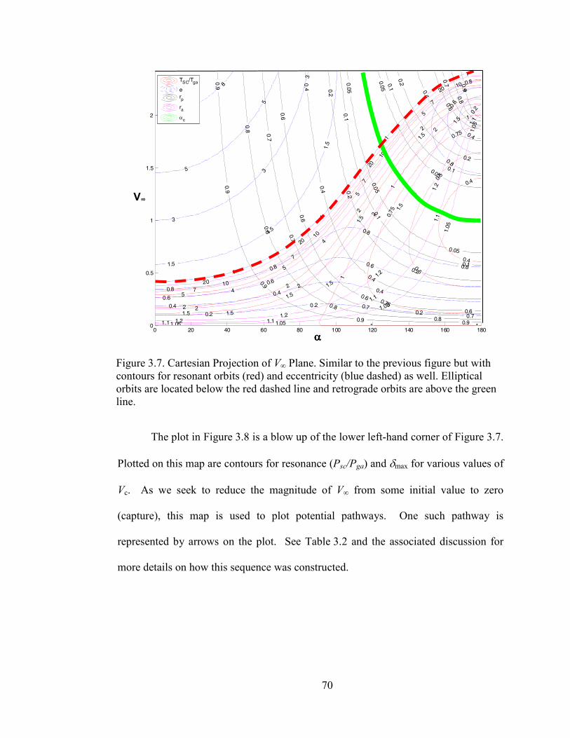
70
Figure 3.7. Cartesian Projection of V∞ Plane. Similar to the previous figure but with contours for resonant orbits (red) and eccentricity (blue dashed) as well. Elliptical orbits are located below the red dashed line and retrograde orbits are above the green line.
The plot in Figure 3.8 is a blow up of the lower left-hand corner of Figure 3.7.
Plotted on this map are contours for resonance (Psc/Pga) and δmax for various values of
Vc. As we seek to reduce the magnitude of V∞ from some initial value to zero
(capture), this map is used to plot potential pathways. One such pathway is
represented by arrows on the plot. See Table 3.2 and the associated discussion for
more details on how this sequence was constructed.
0 20 40 60 80 100 120 140 160 1800
0.5
1
1.5
2
0.4
0.4
0.5
0.5
0.75
0.75
0.75
1
1
1
1 1
1.5
1.5
1.5
1.5
2
2
2
2
5
5
5
5
10
10
10
10
α
V∞
0.2
0.2
0.2
0.2
0.4
0.40.4
0.4
0.6
0.6
0.6
0.6
0.8
0.8
0.8
0.8
0.8
0.8
1
1
1
1
1.5
1.5
1.5
3
3
3
5
5
8
0.0
5
0.0
5
0.05
0.0
5
0.05
0. 1
0.1
0.1
0.1
0.1
0.2
0.2
0.2
0.2
0.2
0. 4
0.4
0.4
0.4
0.6
0.6
0.6
0.6
0.6
0.7
0.7
0.7
0.7
0.7
0.8
0.8
0.8
0.8
0.8
0.9
0.9
0.9
0.90.9
0.9
1.05 1.05
1.05
1.0
5
1.0
5
1.1 1.1
1.1
1.1
1.1
1.21.2
1.2
1.2
1.5
1.5
1.5
1.5
2
2
2
2
4
4
4
4
7
7
7
7
20
20
20
20
0
0
TSC/Tga
e
rp
ra
αc
V∞
αααα
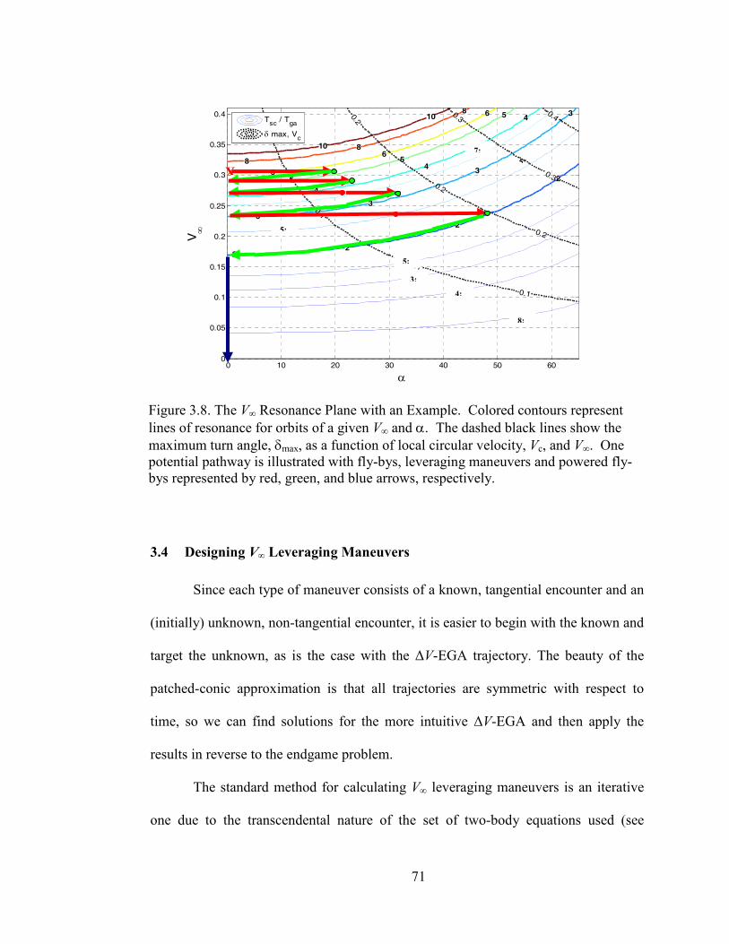
71
0 10 20 30 40 50 600
0.05
0.1
0.15
0.2
0.25
0.3
0.35
0.4
22
2
2
3
3
3
3
4
4
4
5
5
5
6
6
6
8
8
8
10
10
α
V∞
0.1
0.1
0.1
0.1
0.2
0.2
0.2
0.3
0.3
0.4Tsc
/ Tga
δ max, Vc
Figure 3.8. The V∞ Resonance Plane with an Example. Colored contours represent
lines of resonance for orbits of a given V∞ and α. The dashed black lines show the
maximum turn angle, δmax, as a function of local circular velocity, Vc, and V∞. One potential pathway is illustrated with fly-bys, leveraging maneuvers and powered fly-bys represented by red, green, and blue arrows, respectively.
3.4 Designing V∞ Leveraging Maneuvers
Since each type of maneuver consists of a known, tangential encounter and an
(initially) unknown, non-tangential encounter, it is easier to begin with the known and
target the unknown, as is the case with the ∆V-EGA trajectory. The beauty of the
patched-conic approximation is that all trajectories are symmetric with respect to
time, so we can find solutions for the more intuitive ∆V-EGA and then apply the
results in reverse to the endgame problem.
The standard method for calculating V∞ leveraging maneuvers is an iterative
one due to the transcendental nature of the set of two-body equations used (see
X
7:
5:
5:
5:
3:
4:
8:
72
Hollenbeck, 1975). After the spacecraft is launched to a slightly longer than resonant
orbit, a guess is made at the value of a burn (∆VDSM) performed anti-parallel at
aphelion. The trajectory is then propagated to where it intersects Earth’s orbit, both
before and after perihelion. The Earth is then propagated to see if a reencounter
occurs at either point. If not then ∆VDSM is modified, and the process is repeated until
they converge. See Sims (1997) for a more detailed description.
V∞ leveraging analyses found in the literature focus on tangential transfers
where the orbits of the spacecraft and gravity-assist body are tangent to begin or end
the maneuver. This is because a tangential transfer results in the greatest change in
V∞ for a given transfer orbit size. However, occasionally it is more desirable to
perform a non-tangential transfer (α ≠ 0 at either end), particularly in sequences of
leveraging maneuvers where Vc of the moon is low, which makes it difficult to bend α
back to zero without requiring multiple fly-bys and a long TOF.
3.4.1 The Lambert Solution Technique
In order to more completely explore the trade space, a different approach to
leveraging design was used. We desired to free the constraints on the location and
direction of ∆VDSM. To do so a universal variables solution to Lambert’s Problem was
implemented in MATLAB (see Section 2.1.3) This was done by first propagating the
orbits of the gravity-assist body and the spacecraft to produce a specified number of
ephemeris points per orbit (nominally 360). Next, the program loops through every
combination of starting points on the spacecraft orbit and targets points on the
gravity-assist body’s orbit using the Lambert Solver to find the ∆V direction and
magnitude required to complete the transfer.
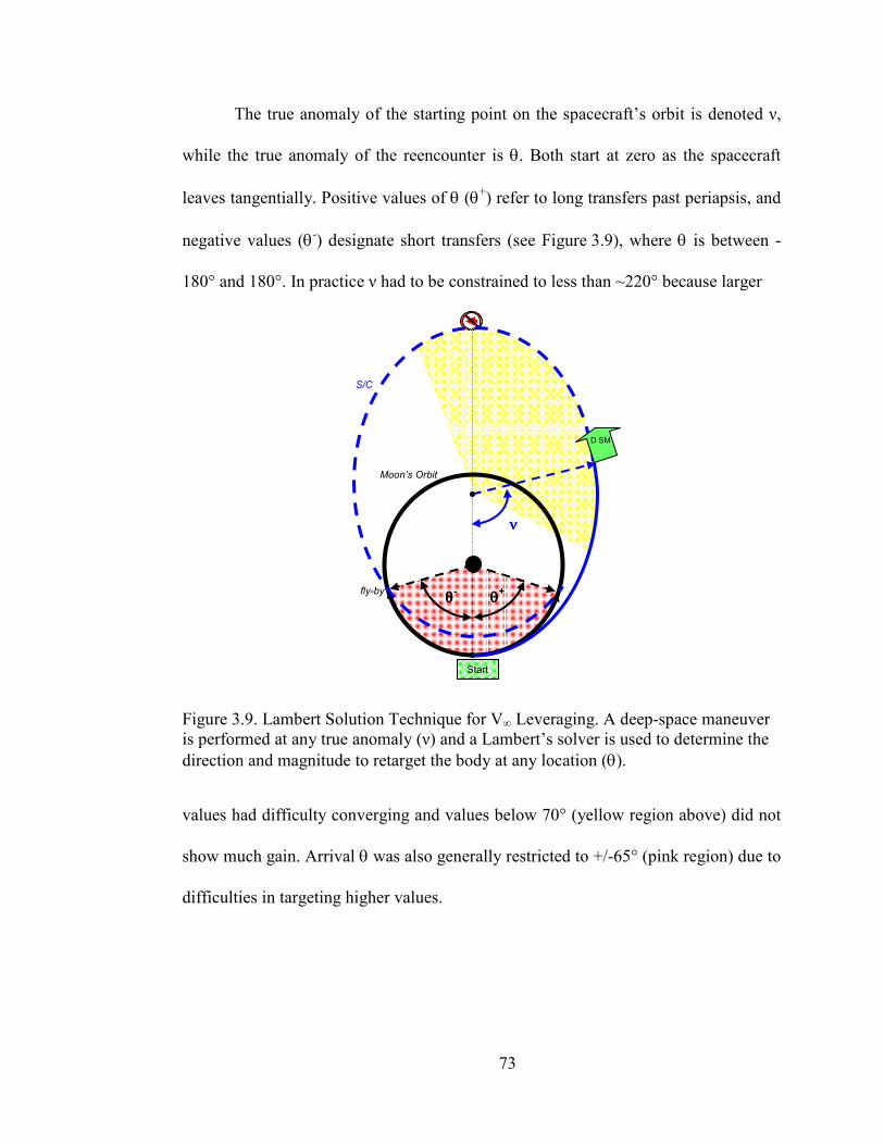
73
The true anomaly of the starting point on the spacecraft’s orbit is denoted ν,
while the true anomaly of the reencounter is θ. Both start at zero as the spacecraft
leaves tangentially. Positive values of θ (θ+) refer to long transfers past periapsis, and
negative values (θ-) designate short transfers (see Figure 3.9), where θ is between -
180° and 180°. In practice ν had to be constrained to less than ~220° because larger
Figure 3.9. Lambert Solution Technique for V∞ Leveraging. A deep-space maneuver is performed at any true anomaly (ν) and a Lambert’s solver is used to determine the
direction and magnitude to retarget the body at any location (θ).
values had difficulty converging and values below 70° (yellow region above) did not
show much gain. Arrival θ was also generally restricted to +/-65° (pink region) due to
difficulties in targeting higher values.
fly-by
Start
Moon’s Orbit
S/C
νννν
θθθθ- θθθθ+
D SM
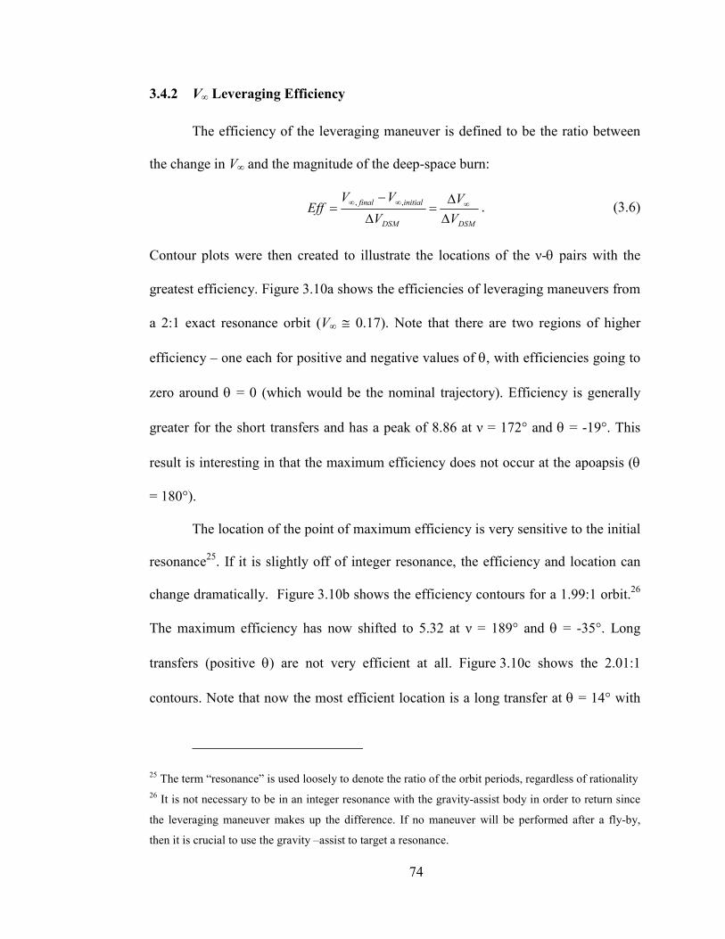
74
3.4.2 V∞ Leveraging Efficiency
The efficiency of the leveraging maneuver is defined to be the ratio between
the change in V∞ and the magnitude of the deep-space burn:
DSMDSM
initialfinal
V
V
V
VVEff
∆
∆=
∆
−= ∞∞∞ ,,
. (3.6)
Contour plots were then created to illustrate the locations of the ν-θ pairs with the
greatest efficiency. Figure 3.10a shows the efficiencies of leveraging maneuvers from
a 2:1 exact resonance orbit (V∞ ≅ 0.17). Note that there are two regions of higher
efficiency – one each for positive and negative values of θ, with efficiencies going to
zero around θ = 0 (which would be the nominal trajectory). Efficiency is generally
greater for the short transfers and has a peak of 8.86 at ν = 172° and θ = -19°. This
result is interesting in that the maximum efficiency does not occur at the apoapsis (θ
= 180°).
The location of the point of maximum efficiency is very sensitive to the initial
resonance25. If it is slightly off of integer resonance, the efficiency and location can
change dramatically. Figure 3.10b shows the efficiency contours for a 1.99:1 orbit.26
The maximum efficiency has now shifted to 5.32 at ν = 189° and θ = -35°. Long
transfers (positive θ) are not very efficient at all. Figure 3.10c shows the 2.01:1
contours. Note that now the most efficient location is a long transfer at θ = 14° with
25 The term “resonance” is used loosely to denote the ratio of the orbit periods, regardless of rationality
26 It is not necessary to be in an integer resonance with the gravity-assist body in order to return since
the leveraging maneuver makes up the difference. If no maneuver will be performed after a fly-by,
then it is crucial to use the gravity –assist to target a resonance.
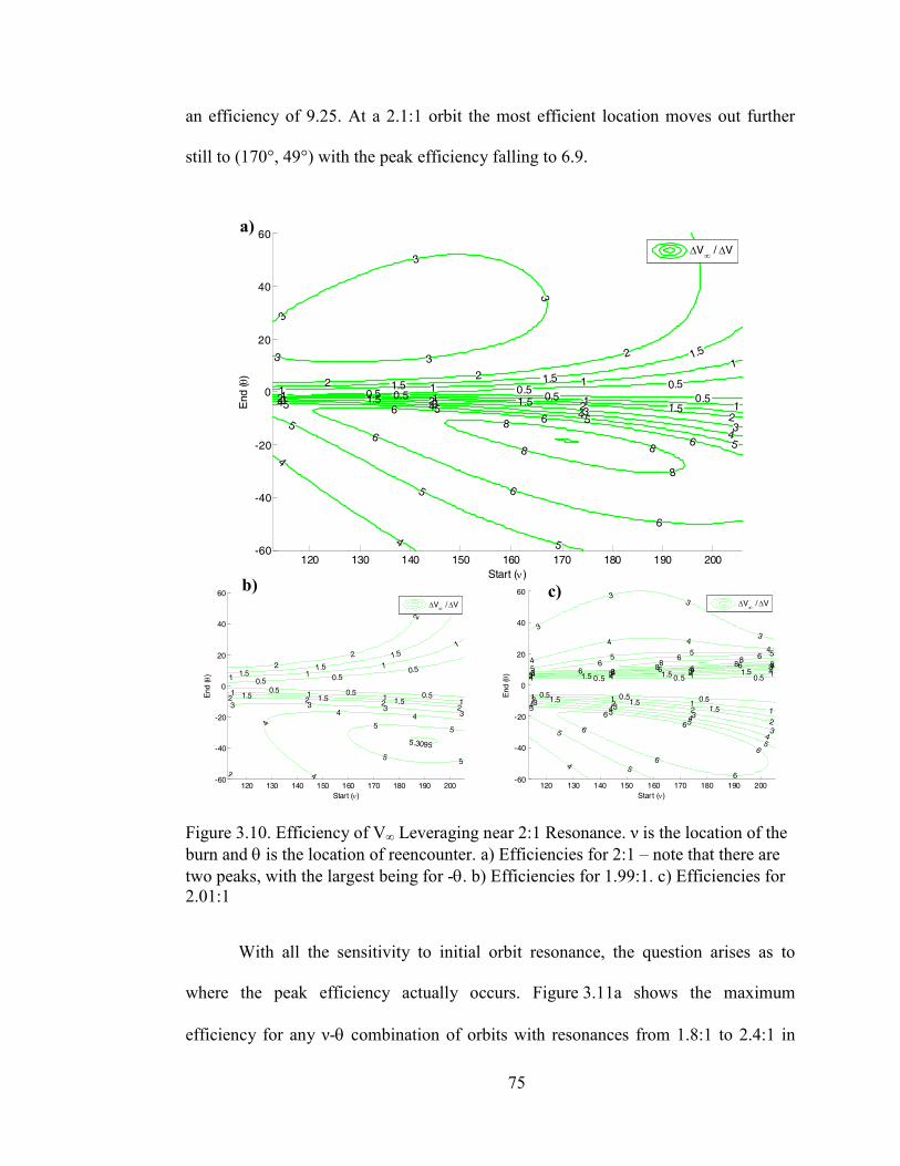
75
an efficiency of 9.25. At a 2.1:1 orbit the most efficient location moves out further
still to (170°, 49°) with the peak efficiency falling to 6.9.
Figure 3.10. Efficiency of V∞ Leveraging near 2:1 Resonance. ν is the location of the
burn and θ is the location of reencounter. a) Efficiencies for 2:1 – note that there are
two peaks, with the largest being for -θ. b) Efficiencies for 1.99:1. c) Efficiencies for 2.01:1
With all the sensitivity to initial orbit resonance, the question arises as to
where the peak efficiency actually occurs. Figure 3.11a shows the maximum
efficiency for any ν-θ combination of orbits with resonances from 1.8:1 to 2.4:1 in
120 130 140 150 160 170 180 190 200-60
-40
-20
0
20
40
60
0.5 0.5 0.5
0.5 0.5 0.5
1 1 1 1
1 11
1
1.5 1.5 1.5
1.5 1.51.5
2 2 2 2
2 22
2
3
33
3
3 3 33
33
3
3
4
4
4 44
4 4 44
44
4
4
5
5
5
55 5
5 5 55
5 5
5
5
666
6 66
6
6
6
6
6
6
888 8
Start (ν)
End (
θ)
∞
∆V∞ / ∆V
120 130 140 150 160 170 180 190 200-60
-40
-20
0
20
40
60
0.5 0.50.5
0.5 0.5 0.5
11
1
1
1 1 11
1.5
1.5
1.51.5
1.5 1.5 1.5
2
2
2
2 2 22
3
3 3 33
4
4
44
55
55
5.3095
Start (ν)
End (
θ)
∆V∞ / ∆V
120 130 140 150 160 170 180 190 200-60
-40
-20
0
20
40
60
0.50.50.5 0.5 0.5 0.5
1 11
1
1 1 1 1
1.51.5
1.5
1.5 1.51.5
2
2
22
2 2 22
3
3
333
3 33
3
4
4
4 44
4
5
5
5
5 55
56
66
6
6
6
8
8
8
8
Start (ν)
End (
θ)
∞
∆V∞ / ∆V
a)
b) c)
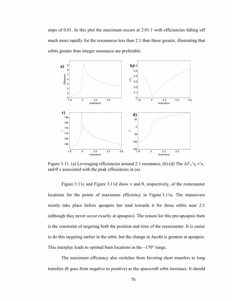
76
steps of 0.01. In this plot the maximum occurs at 2.01:1 with efficiencies falling off
much more rapidly for the resonances less than 2:1 than those greater, illustrating that
orbits greater than integer resonance are preferable.
Figure 3.11. (a) Leveraging efficiencies around 2:1 resonance, (b)-(d) The ∆V∞’s, ν’s,
and θ’s associated with the peak efficiencies in (a).
Figure 3.11c and Figure 3.11d show ν and θ, respectively, of the reencounter
locations for the points of maximum efficiency in Figure 3.11a. The maneuvers
mostly take place before apoapsis but tend towards it for those orbits near 2:1
(although they never occur exactly at apoapsis). The reason for this pre-apoapsis burn
is the constraint of targeting both the position and time of the reencounter. It is easier
to do this targeting earlier in the orbit, but the change in Jacobi is greatest at apoapsis.
This interplay leads to optimal burn locations in the ~170° range.
The maximum efficiency also switches from favoring short transfers to long
transfers (θ goes from negative to positive) as the spacecraft orbit increases. It should
1.8 2 2.2 2.4 2.6
160
165
170
175
180
185
resonance
ν
1.8 2 2.2 2.4-150
-100
-50
0
50
resonance
θ
1.8 2 2.2 2.42
3
4
5
6
7
8
9
resonance
Effic
iency
1.8 2 2.2 2.4 2.60
0.1
0.2
0.3
0.4
0.5
0.6
resonance
∆V
∞
a) b)
c) d)
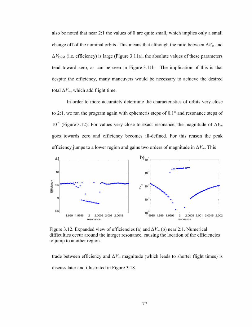
77
also be noted that near 2:1 the values of θ are quite small, which implies only a small
change off of the nominal orbits. This means that although the ratio between ∆V∞ and
∆VDSM (i.e. efficiency) is large (Figure 3.11a), the absolute values of these parameters
tend toward zero, as can be seen in Figure 3.11b. The implication of this is that
despite the efficiency, many maneuvers would be necessary to achieve the desired
total ∆V∞, which add flight time.
In order to more accurately determine the characteristics of orbits very close
to 2:1, we ran the program again with ephemeris steps of 0.1° and resonance steps of
10-4 (Figure 3.12). For values very close to exact resonance, the magnitude of ∆V∞
goes towards zero and efficiency becomes ill-defined. For this reason the peak
efficiency jumps to a lower region and gains two orders of magnitude in ∆V∞. This
1.999 1.9995 2 2.0005 2.001 2.0015
8.5
9
9.5
10
resonance
Eff
icie
ncy
1.9985 1.999 1.9995 2 2.0005 2.001 2.0015 2.00210
-5
10-4
10-3
10-2
10-1
resonance
∆V
∞
Figure 3.12. Expanded view of efficiencies (a) and ∆V∞ (b) near 2:1. Numerical difficulties occur around the integer resonance, causing the location of the efficiencies to jump to another region.
trade between efficiency and ∆V∞ magnitude (which leads to shorter flight times) is
discuss later and illustrated in Figure 3.18.
a) b)
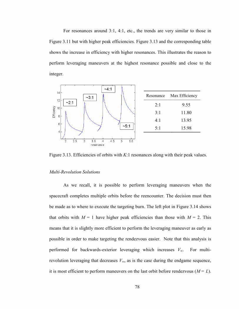
78
For resonances around 3:1, 4:1, etc., the trends are very similar to those in
Figure 3.11 but with higher peak efficiencies. Figure 3.13 and the corresponding table
shows the increase in efficiency with higher resonances. This illustrates the reason to
perform leveraging maneuvers at the highest resonance possible and close to the
integer.
Resonance Max Efficiency
2:1 9.55
3:1 11.80
4:1 13.95
5:1 15.98
Figure 3.13. Efficiencies of orbits with K:1 resonances along with their peak values.
Multi-Revolution Solutions
As we recall, it is possible to perform leveraging maneuvers when the
spacecraft completes multiple orbits before the reencounter. The decision must then
be made as to where to execute the targeting burn. The left plot in Figure 3.14 shows
that orbits with M = 1 have higher peak efficiencies than those with M = 2. This
means that it is slightly more efficient to perform the leveraging maneuver as early as
possible in order to make targeting the rendezvous easier. Note that this analysis is
performed for backwards-exterior leveraging which increases V∞. For multi-
revolution leveraging that decreases V∞, as is the case during the endgame sequence,
it is most efficient to perform maneuvers on the last orbit before rendezvous (M = L).
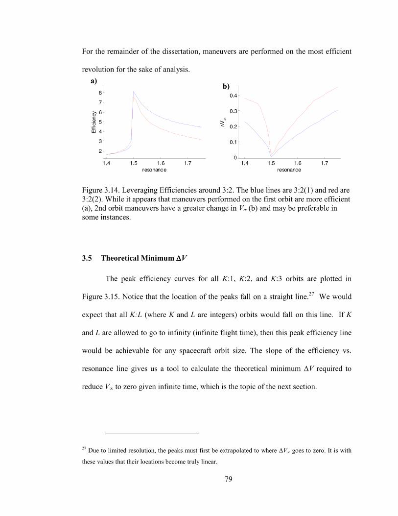
79
For the remainder of the dissertation, maneuvers are performed on the most efficient
revolution for the sake of analysis.
Figure 3.14. Leveraging Efficiencies around 3:2. The blue lines are 3:2(1) and red are 3:2(2). While it appears that maneuvers performed on the first orbit are more efficient (a), 2nd orbit maneuvers have a greater change in V∞ (b) and may be preferable in some instances.
3.5 Theoretical Minimum ∆∆∆∆V
The peak efficiency curves for all K:1, K:2, and K:3 orbits are plotted in
Figure 3.15. Notice that the location of the peaks fall on a straight line.27 We would
expect that all K:L (where K and L are integers) orbits would fall on this line. If K
and L are allowed to go to infinity (infinite flight time), then this peak efficiency line
would be achievable for any spacecraft orbit size. The slope of the efficiency vs.
resonance line gives us a tool to calculate the theoretical minimum ∆V required to
reduce V∞ to zero given infinite time, which is the topic of the next section.
27 Due to limited resolution, the peaks must first be extrapolated to where ∆V∞ goes to zero. It is with
these values that their locations become truly linear.
1.4 1.5 1.6 1.7
2
3
4
5
6
7
8
resonance
Eff
icie
ncy
1.4 1.5 1.6 1.70
0.1
0.2
0.3
0.4
resonance
∆V
∞
b) a)
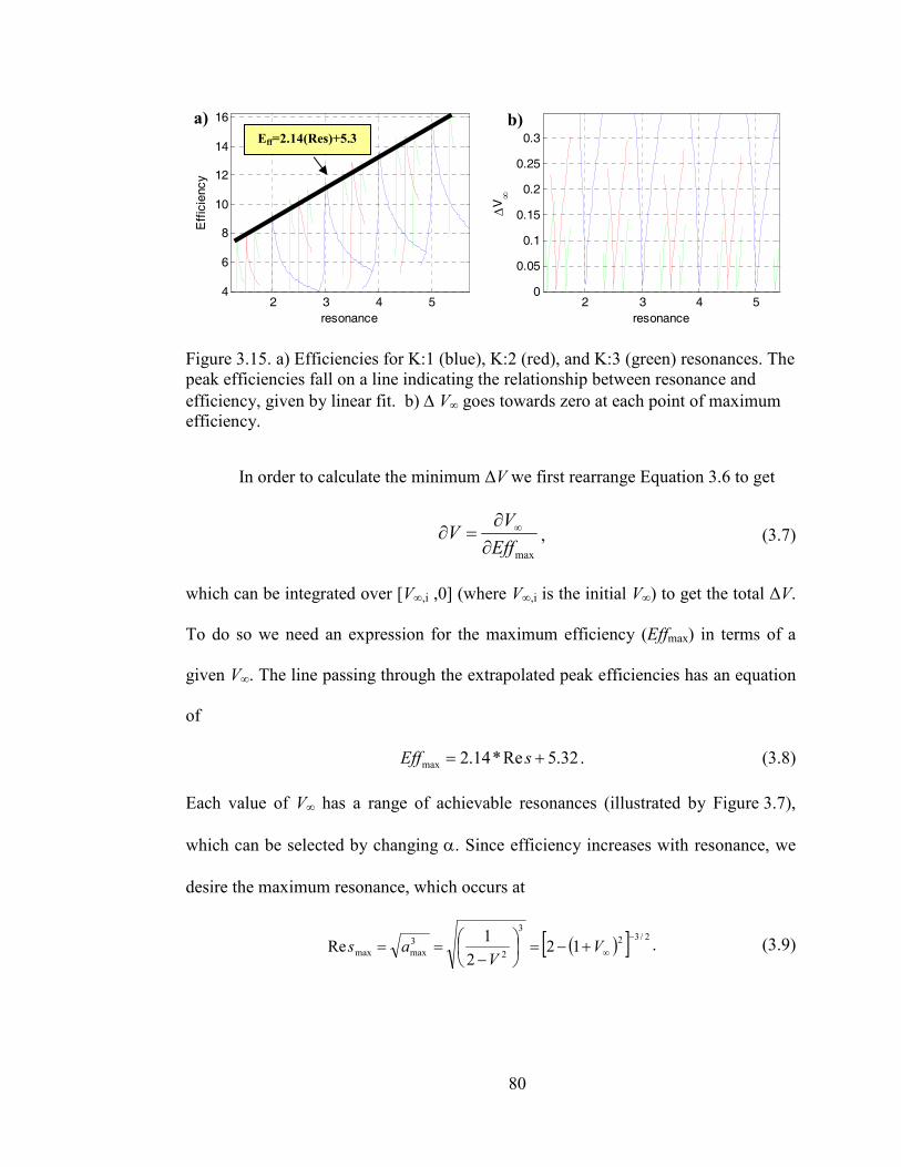
80
2 3 4 54
6
8
10
12
14
16
resonance
Eff
icie
ncy
2 3 4 50
0.05
0.1
0.15
0.2
0.25
0.3
resonance
∆V
∞
Figure 3.15. a) Efficiencies for K:1 (blue), K:2 (red), and K:3 (green) resonances. The peak efficiencies fall on a line indicating the relationship between resonance and
efficiency, given by linear fit. b) ∆ V∞ goes towards zero at each point of maximum efficiency.
In order to calculate the minimum ∆V we first rearrange Equation 3.6 to get
maxEff
VV
∂
∂=∂ ∞
, (3.7)
which can be integrated over [V∞,i ,0] (where V∞,i is the initial V∞) to get the total ∆V.
To do so we need an expression for the maximum efficiency (Effmax) in terms of a
given V∞. The line passing through the extrapolated peak efficiencies has an equation
of
32.5Re*14.2max += sEff . (3.8)
Each value of V∞ has a range of achievable resonances (illustrated by Figure 3.7),
which can be selected by changing α. Since efficiency increases with resonance, we
desire the maximum resonance, which occurs at
( )[ ] 2/32
3
2
3
maxmax 122
1Re
−
∞+−=
−
== VV
as . (3.9)
Eff=2.14(Res)+5.3
a) b)
81
Now we can write an expression for Effmax(V∞) by substituting Equation 3.928
into Equation 3.8 and by defining the equation
[ ] 32.5)1(214.22/32
max ++−=−
∞VEff . (3.10)
The integral for the minimum ∆V can now be expressed as
∫∞
∞=∆iV
dVEff
V,
0max
min
1. (3.11)
The integral above can be solved numerically and is depicted by the blue line
in Figure 3.16. We would begin to create the trajectory to achieve this minimum ∆V
by using fly-bys to bring α to zero and to maximize the resonance for the initial V∞.
The maximum resonance could be something like 186:37, but that is inconsequential
since time is not restricted. On one of the 37 orbits, an infinitesimal ∆V would be
applied to bring about a reduction in V∞ as efficiently as possible. This process would
then continue in infinitesimal steps until V∞ goes to zero. The total ∆V required to
reduce any V∞ above 0.41 (but below 2.41) is 0.034. This is because the orbits above
V∞ = 0.41 can be made to perform their leveraging maneuvers at infinity for zero fuel.
28 Note that Resmax and Effmax go to infinity as V∞ approaches √2 -1 (~0.41).
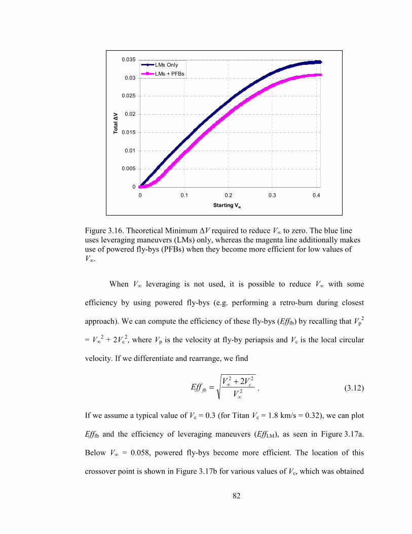
82
0
0.005
0.01
0.015
0.02
0.025
0.03
0.035
0 0.1 0.2 0.3 0.4
Starting V∞∞∞∞
To
tal ∆
V
LMs Only
LMs + PFBs
Figure 3.16. Theoretical Minimum ∆V required to reduce V∞ to zero. The blue line uses leveraging maneuvers (LMs) only, whereas the magenta line additionally makes use of powered fly-bys (PFBs) when they become more efficient for low values of V∞.
When V∞ leveraging is not used, it is possible to reduce V∞ with some
efficiency by using powered fly-bys (e.g. performing a retro-burn during closest
approach). We can compute the efficiency of these fly-bys (Efffb) by recalling that Vp2
= V∞2 + 2Vc
2, where Vp is the velocity at fly-by periapsis and Vc is the local circular
velocity. If we differentiate and rearrange, we find
2
22 2
∞
∞ +=
V
VVEff c
fb . (3.12)
If we assume a typical value of Vc = 0.3 (for Titan Vc = 1.8 km/s = 0.32), we can plot
Efffb and the efficiency of leveraging maneuvers (EffLM), as seen in Figure 3.17a.
Below V∞ = 0.058, powered fly-bys become more efficient. The location of this
crossover point is shown in Figure 3.17b for various values of Vc, which was obtained
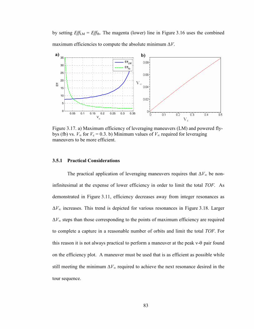
83
by setting EffLM = Efffb. The magenta (lower) line in Figure 3.16 uses the combined
maximum efficiencies to compute the absolute minimum ∆V.
0.05 0.1 0.15 0.2 0.25 0.3 0.350
5
10
15
20
25
30
35
V∞
Eff
EffLM
Efffb
Figure 3.17. a) Maximum efficiency of leveraging maneuvers (LM) and powered fly-bys (fb) vs. V∞ for Vc = 0.3. b) Minimum values of V∞ required for leveraging maneuvers to be more efficient.
3.5.1 Practical Considerations
The practical application of leveraging maneuvers requires that ∆V∞ be non-
infinitesimal at the expense of lower efficiency in order to limit the total TOF. As
demonstrated in Figure 3.11, efficiency decreases away from integer resonances as
∆V∞ increases. This trend is depicted for various resonances in Figure 3.18. Larger
∆V∞ steps than those corresponding to the points of maximum efficiency are required
to complete a capture in a reasonable number of orbits and limit the total TOF. For
this reason it is not always practical to perform a maneuver at the peak ν-θ pair found
on the efficiency plot. A maneuver must be used that is as efficient as possible while
still meeting the minimum ∆V∞ required to achieve the next resonance desired in the
tour sequence.
b) a)
Vc
V∞
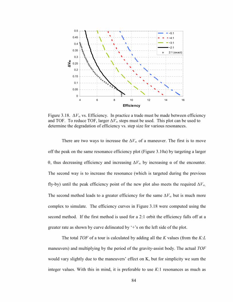
84
0
0.05
0.1
0.15
0.2
0.25
0.3
0.35
0.4
0.45
0.5
4 6 8 10 12 14 16
Efficiency
∆V
∞∞ ∞∞
~5:1
~4:1
~3:1
~2:1
2:1 (exact)
Figure 3.18. ∆V∞ vs. Efficiency. In practice a trade must be made between efficiency and TOF. To reduce TOF, larger ∆V∞ steps must be used. This plot can be used to determine the degradation of efficiency vs. step size for various resonances.
There are two ways to increase the ∆V∞ of a maneuver. The first is to move
off the peak on the same resonance efficiency plot (Figure 3.10a) by targeting a larger
θ, thus decreasing efficiency and increasing ∆V∞ by increasing α of the encounter.
The second way is to increase the resonance (which is targeted during the previous
fly-by) until the peak efficiency point of the new plot also meets the required ∆V∞.
The second method leads to a greater efficiency for the same ∆V∞ but is much more
complex to simulate. The efficiency curves in Figure 3.18 were computed using the
second method. If the first method is used for a 2:1 orbit the efficiency falls off at a
greater rate as shown by curve delineated by ‘+’s on the left side of the plot.
The total TOF of a tour is calculated by adding all the K values (from the K:L
maneuvers) and multiplying by the period of the gravity-assist body. The actual TOF
would vary slightly due to the maneuvers’ effect on K, but for simplicity we sum the
integer values. With this in mind, it is preferable to use K:1 resonances as much as

85
possible since they are ~50% more efficient than K:2 resonances of equivalent
duration and even more efficient than for larger L values.
3.6 Global Search Methodology
An endgame tour sequence begins with a spacecraft in an elliptical orbit about
the central body and in some (usually large) resonance with the gravity-assist body.
A series of reducing resonances are targeted using alternating fly-bys (both un-
powered and powered) and V∞ leveraging maneuvers until V∞ = 0. For our purposes
we reverse the process by beginning with V∞ = 0 and work outwards towards the
large resonance. As an arbitrary metric, we chose an end point of a 6:1 orbit with V∞
= 0.3027 and α = 0. The total ∆V and TOF for the tour sequence is accumulated for
comparisons.
To begin, a powered fly-by (more efficient for low V∞’s) is used to boost the
spacecraft to a starting resonant orbit. Then a leveraging maneuver is performed
around apoapsis to target the next fly-by at a new location with a new, higher V∞
corresponding to the next resonance in the desired sequence. The value of the V∞
being targeted is calculated by
12 3/2
, −−= −∞ newnew RV . (3.13)
The act of performing the leveraging maneuver also brings the orbits out of
tangency, increasing α at the new encounter which can be approximated29 by
29 This is an approximation because the leveraging maneuver also changes the resonance by a few
percent thus making R not a constant in the derivation. During our simulations we calculate the true
value of α numerically.
86
−−=
∞
−∞−
new
newnew
V
RV
,
3/22
,1
2
1cosα . (3.14)
Equations 3.13 and 3.14 are each just rearrangements of Equation 3.5 except that
Equation 3.5 has α set to zero. We bring these equations into agreement and achieve
the new resonance by using the fly-by to bend the V∞ vector and to rotate α back to
zero. If α is greater than δmax, an intermediate α and R must be chosen as a “phasing
orbit” until α can be reduced to zero on a subsequent fly-by. Phasing orbits increase
the tour duration but not the total ∆V. Sometimes multiple phasing orbits may be
required. Once the orbits are again tangent, the process is repeated to target the next
resonance until the desired end point is achieved.
3.6.1 Simulations
Endgame tours can be constructed by a limitless number of combinations of
resonance orbits, leveraging maneuvers, fly-bys, phasing orbits, etc. One such
sequence constructed “by hand” is depicted in Table 3.2 below and on the V∞ Plane in
Figure 3.8, (which is repeated as Figure 3.19 below for convenience). This tour uses
the following resonant orbits: 2:1, 3:1, 4:1, 5:1, 6:1. The tour begins with a powered
fly-by to boost the spacecraft to a 2:1 orbit. Around apoapsis a leveraging maneuver
is applied to change the V∞ of the next encounter from 0.171 to 0.233. The maneuver
also causes α to go from 0° to 48.6°. This is illustrated by following the 2:1
resonance line in Figure 3.19 starting at α = 0° and V∞ = 0.17 up until the line crosses
V∞ = 0.233 (which corresponds to a 3:1 orbit when α = 0) at α = 48.6°.
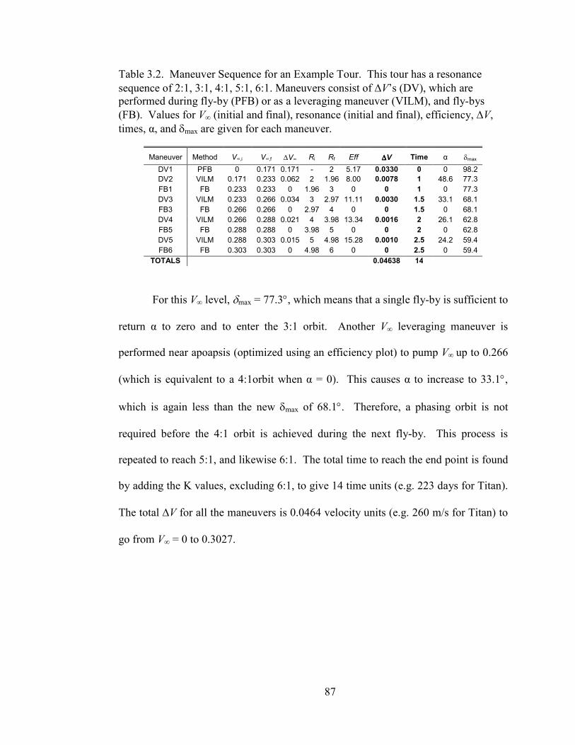
87
Table 3.2. Maneuver Sequence for an Example Tour. This tour has a resonance
sequence of 2:1, 3:1, 4:1, 5:1, 6:1. Maneuvers consist of ∆V’s (DV), which are performed during fly-by (PFB) or as a leveraging maneuver (VILM), and fly-bys
(FB). Values for V∞ (initial and final), resonance (initial and final), efficiency, ∆V,
times, α, and δmax are given for each maneuver.
Maneuver Method V∞,i V∞,f ∆V∞ Ri Rf Eff ∆∆∆∆V Time α δmax
DV1 PFB 0 0.171 0.171 - 2 5.17 0.0330 0 0 98.2
DV2 VILM 0.171 0.233 0.062 2 1.96 8.00 0.0078 1 48.6 77.3
FB1 FB 0.233 0.233 0 1.96 3 0 0 1 0 77.3
DV3 VILM 0.233 0.266 0.034 3 2.97 11.11 0.0030 1.5 33.1 68.1
FB3 FB 0.266 0.266 0 2.97 4 0 0 1.5 0 68.1
DV4 VILM 0.266 0.288 0.021 4 3.98 13.34 0.0016 2 26.1 62.8
FB5 FB 0.288 0.288 0 3.98 5 0 0 2 0 62.8
DV5 VILM 0.288 0.303 0.015 5 4.98 15.28 0.0010 2.5 24.2 59.4
FB6 FB 0.303 0.303 0 4.98 6 0 0 2.5 0 59.4
TOTALS 0.04638 14
For this V∞ level, δmax = 77.3°, which means that a single fly-by is sufficient to
return α to zero and to enter the 3:1 orbit. Another V∞ leveraging maneuver is
performed near apoapsis (optimized using an efficiency plot) to pump V∞ up to 0.266
(which is equivalent to a 4:1orbit when α = 0). This causes α to increase to 33.1°,
which is again less than the new δmax of 68.1°. Therefore, a phasing orbit is not
required before the 4:1 orbit is achieved during the next fly-by. This process is
repeated to reach 5:1, and likewise 6:1. The total time to reach the end point is found
by adding the K values, excluding 6:1, to give 14 time units (e.g. 223 days for Titan).
The total ∆V for all the maneuvers is 0.0464 velocity units (e.g. 260 m/s for Titan) to
go from V∞ = 0 to 0.3027.
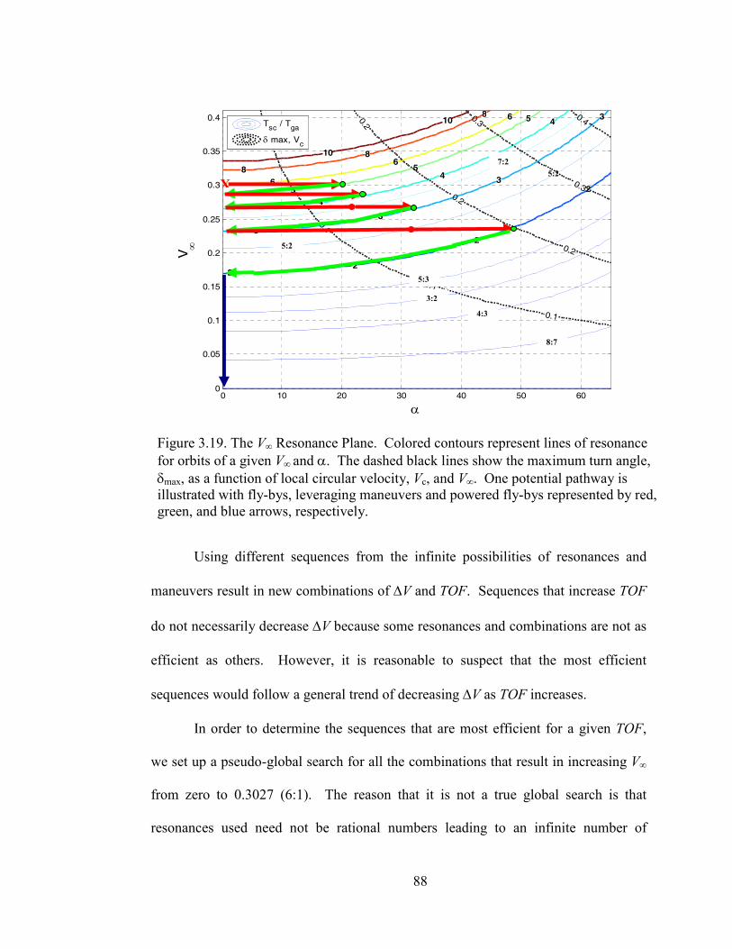
88
0 10 20 30 40 50 600
0.05
0.1
0.15
0.2
0.25
0.3
0.35
0.4
22
2
2
3
3
3
3
4
4
4
5
5
5
6
6
6
8
8
8
10
10
α
V∞
0.1
0.1
0.1
0.1
0.2
0.2
0.2
0.3
0.3
0.4Tsc
/ Tga
δ max, Vc
Figure 3.19. The V∞ Resonance Plane. Colored contours represent lines of resonance
for orbits of a given V∞ and α. The dashed black lines show the maximum turn angle,
δmax, as a function of local circular velocity, Vc, and V∞. One potential pathway is illustrated with fly-bys, leveraging maneuvers and powered fly-bys represented by red, green, and blue arrows, respectively.
Using different sequences from the infinite possibilities of resonances and
maneuvers result in new combinations of ∆V and TOF. Sequences that increase TOF
do not necessarily decrease ∆V because some resonances and combinations are not as
efficient as others. However, it is reasonable to suspect that the most efficient
sequences would follow a general trend of decreasing ∆V as TOF increases.
In order to determine the sequences that are most efficient for a given TOF,
we set up a pseudo-global search for all the combinations that result in increasing V∞
from zero to 0.3027 (6:1). The reason that it is not a true global search is that
resonances used need not be rational numbers leading to an infinite number of
X
7:2
5:2
5:3
5:2
3:2
4:3
8:7
89
pathways. To thoroughly explore the trade space, we set up a Monte Carlo-like
algorithm that uses random number generators to select the next maneuver of a
sequence from a range or set of possibilities.
The algorithm begins by assuming that V∞ = 0 (parabolic orbit) and Vc = 0.3
(Titan-like). A random number generator selects K and L values such that K/L = R >
6. They are also restricted to values less than 24, with lower values being more
heavily weighted in order to favor shorter flight times. The required ∆V is then
calculated for a powered fly-by to reach the generated R.
Next the number generator selects a resonance and associated V∞ to target. A
V∞ leveraging efficiency plot such as the one in Figure 3.10a is generated for the
initial resonance. The most efficient ν-θ pair that also results in the desired ∆V∞ is
then selected as the next leveraging maneuver. The associated ∆V and duration (~K)
is added to the totals, and α for the next encounter is calculated. If α is less than δmax,
then the fly-by is used to bend α back to zero, and the process is repeated. If α is
greater than δmax, then a choice is made whether to target a phasing orbit, use a
powered fly-by, or to begin the next leveraging maneuver from a non-tangential orbit
(using the smallest α achievable with the one fly-by).
If a phasing orbit is used, then a script is called that selects the intermediate
resonance to use from the range dictated by α and δmax. A heavier weight is placed on
resonances with lower K values as well as those that use a larger δ so that α can reach
zero in as few phasing orbits as possible. This sequence selection and calculation
process continues until R = 6 and α = 0. The total ∆V, TOF, and resonance sequence
are output for each iteration.
90
The algorithm just described can be tailored to obey one of three overarching
rules: (1) No Crossing δmax (NX) - the use of phasing orbits is disallowed by requiring
that next target resonance in a sequence does not cause α to cross the δmax line for the
given value of Vc on the plot shown in Figure 3.19. This means that the orbits can
always return to tangency at the cost of smaller ∆V∞ steps and more leveraging
maneuvers. (2) Phasing Orbits (PH) - crossing of the δmax line is allowed but requires
that phasing orbits be used until α returns to zero before another leveraging maneuver
can be performed. The sequence given in Table 3.2 is an example of this rule. (3)
Non-Tangential (NT) - the third overarching rule is opposite from the second one in
that no phasing orbits are allowed and leveraging maneuvers are performed from
orbits that begin from a non-tangential state.
3.7 Results
Our Monte-Carlo simulations generated tens of thousands of unique paths,
most of which are not useful for practical tours as they are either extremely long in
duration, less effective than a direct powered fly-by, or are much less efficient than an
alternate sequence of an equivalent duration. Figure 3.20 is a plot of ∆V vs. TOF for
all the simulated cases with Vc = 0.3. The lowest total ∆V across the range of TOFs
creates a Pareto front indicated by the solid line. This front represents the trade
between fuel and duration in the tour design process.
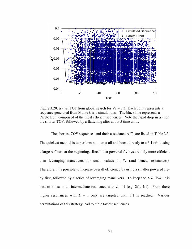
91
0.04
0.05
0.06
0.07
0.08
0.09
0.1
0 20 40 60 80 100
TOF
∆∆ ∆∆V
Simulated Sequence
Pareto Front
Figure 3.20. ∆V vs. TOF from global search for Vc = 0.3. Each point represents a sequence generated from Monte Carlo simulations. The black line represents a
Pareto front comprised of the most efficient sequences. Note the rapid drop in ∆V for the shorter TOFs followed by a flattening after about 5 time units.
The shortest TOF sequences and their associated ∆V’s are listed in Table 3.3.
The quickest method is to perform no tour at all and boost directly to a 6:1 orbit using
a large ∆V burn at the beginning. Recall that powered fly-bys are only more efficient
than leveraging maneuvers for small values of V∞ (and hence, resonances).
Therefore, it is possible to increase overall efficiency by using a smaller powered fly-
by first, followed by a series of leveraging maneuvers. To keep the TOF low, it is
best to boost to an intermediate resonance with L = 1 (e.g. 2:1, 4:1). From there
higher resonances with L = 1 only are targeted until 6:1 is reached. Various
permutations of this strategy lead to the 7 fastest sequences.
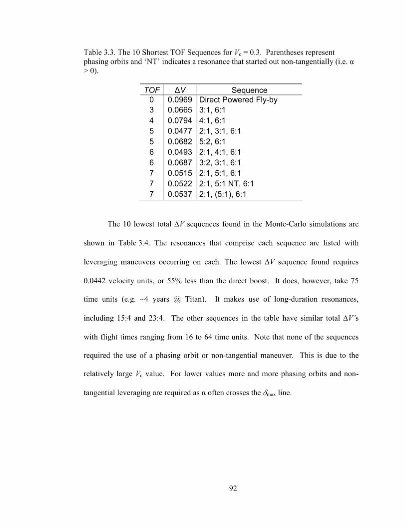
92
Table 3.3. The 10 Shortest TOF Sequences for Vc = 0.3. Parentheses represent phasing orbits and ‘NT’ indicates a resonance that started out non-tangentially (i.e. α > 0).
TOF ∆V Sequence
0 0.0969 Direct Powered Fly-by
3 0.0665 3:1, 6:1
4 0.0794 4:1, 6:1
5 0.0477 2:1, 3:1, 6:1
5 0.0682 5:2, 6:1
6 0.0493 2:1, 4:1, 6:1
6 0.0687 3:2, 3:1, 6:1
7 0.0515 2:1, 5:1, 6:1
7 0.0522 2:1, 5:1 NT, 6:1
7 0.0537 2:1, (5:1), 6:1
The 10 lowest total ∆V sequences found in the Monte-Carlo simulations are
shown in Table 3.4. The resonances that comprise each sequence are listed with
leveraging maneuvers occurring on each. The lowest ∆V sequence found requires
0.0442 velocity units, or 55% less than the direct boost. It does, however, take 75
time units (e.g. ~4 years @ Titan). It makes use of long-duration resonances,
including 15:4 and 23:4. The other sequences in the table have similar total ∆V’s
with flight times ranging from 16 to 64 time units. Note that none of the sequences
required the use of a phasing orbit or non-tangential maneuver. This is due to the
relatively large Vc value. For lower values more and more phasing orbits and non-
tangential leveraging are required as α often crosses the δmax line.
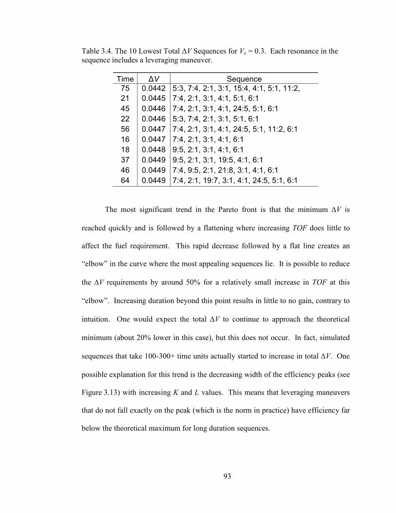
93
Table 3.4. The 10 Lowest Total ∆V Sequences for Vc = 0.3. Each resonance in the sequence includes a leveraging maneuver.
Time ∆V Sequence
75 0.0442 5:3, 7:4, 2:1, 3:1, 15:4, 4:1, 5:1, 11:2,
21 0.0445 7:4, 2:1, 3:1, 4:1, 5:1, 6:1
45 0.0446 7:4, 2:1, 3:1, 4:1, 24:5, 5:1, 6:1
22 0.0446 5:3, 7:4, 2:1, 3:1, 5:1, 6:1
56 0.0447 7:4, 2:1, 3:1, 4:1, 24:5, 5:1, 11:2, 6:1
16 0.0447 7:4, 2:1, 3:1, 4:1, 6:1
18 0.0448 9:5, 2:1, 3:1, 4:1, 6:1
37 0.0449 9:5, 2:1, 3:1, 19:5, 4:1, 6:1
46 0.0449 7:4, 9:5, 2:1, 21:8, 3:1, 4:1, 6:1
64 0.0449 7:4, 2:1, 19:7, 3:1, 4:1, 24:5, 5:1, 6:1
The most significant trend in the Pareto front is that the minimum ∆V is
reached quickly and is followed by a flattening where increasing TOF does little to
affect the fuel requirement. This rapid decrease followed by a flat line creates an
“elbow” in the curve where the most appealing sequences lie. It is possible to reduce
the ∆V requirements by around 50% for a relatively small increase in TOF at this
“elbow”. Increasing duration beyond this point results in little to no gain, contrary to
intuition. One would expect the total ∆V to continue to approach the theoretical
minimum (about 20% lower in this case), but this does not occur. In fact, simulated
sequences that take 100-300+ time units actually started to increase in total ∆V. One
possible explanation for this trend is the decreasing width of the efficiency peaks (see
Figure 3.13) with increasing K and L values. This means that leveraging maneuvers
that do not fall exactly on the peak (which is the norm in practice) have efficiency far
below the theoretical maximum for long duration sequences.
94
To this point we have primarily discussed simulation results for Vc = 0.3
because this work is especially meant to be applicable to the Titan-Saturn system,
where there is only one significant body available for gravity assists and Vc,Titan =
0.32. Changing Vc dramatically alters the control the gravity-assist body has on the
V∞ vector and hence, limits (or enables) orbital parameters after a single fly-by. The
points and Pareto front in Figure 3.20 are a conglomeration of all the sequences
generated, allowing for all three of the overarching rules described in the previous
section. In this case, where Vc = 0.3, the first rule, NX (or no crossing of the δmax
line), is almost always the most beneficial as α rarely approaches the δmax line.
However, if we break the front into those sequences that use phasing (PH), non-
tangential maneuvers (NT), and a mix for Vc = 0.2, we can see in Figure 3.21 that
each strategy can be equally beneficial for reducing the total ∆V and creating an
efficient sequence with none being clearly better than the others.
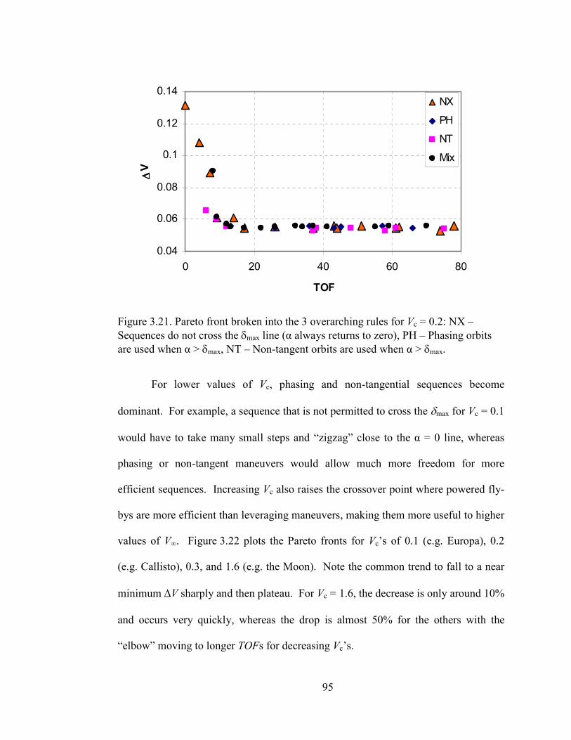
95
0.04
0.06
0.08
0.1
0.12
0.14
0 20 40 60 80
TOF
∆∆ ∆∆V
NX
PH
NT
Mix
Figure 3.21. Pareto front broken into the 3 overarching rules for Vc = 0.2: NX –
Sequences do not cross the δmax line (α always returns to zero), PH – Phasing orbits
are used when α > δmax, NT – Non-tangent orbits are used when α > δmax.
For lower values of Vc, phasing and non-tangential sequences become
dominant. For example, a sequence that is not permitted to cross the δmax for Vc = 0.1
would have to take many small steps and “zigzag” close to the α = 0 line, whereas
phasing or non-tangent maneuvers would allow much more freedom for more
efficient sequences. Increasing Vc also raises the crossover point where powered fly-
bys are more efficient than leveraging maneuvers, making them more useful to higher
values of V∞. Figure 3.22 plots the Pareto fronts for Vc’s of 0.1 (e.g. Europa), 0.2
(e.g. Callisto), 0.3, and 1.6 (e.g. the Moon). Note the common trend to fall to a near
minimum ∆V sharply and then plateau. For Vc = 1.6, the decrease is only around 10%
and occurs very quickly, whereas the drop is almost 50% for the others with the
“elbow” moving to longer TOFs for decreasing Vc’s.
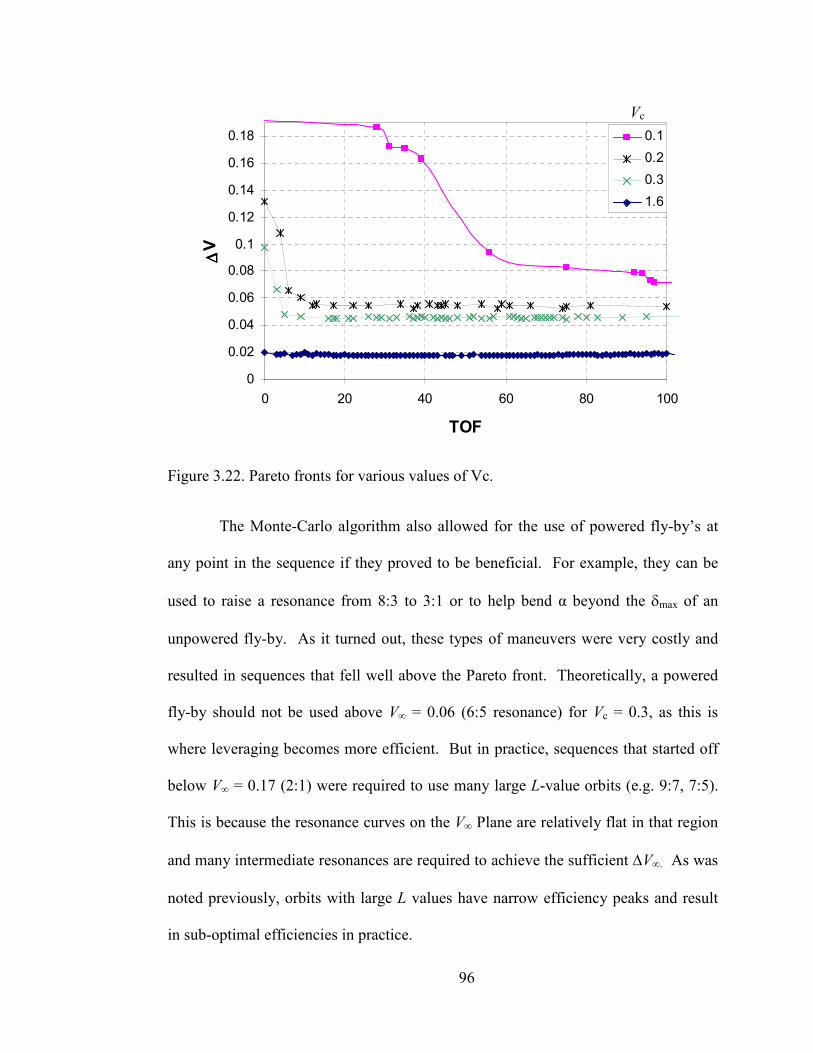
96
0
0.02
0.04
0.06
0.08
0.1
0.12
0.14
0.16
0.18
0 20 40 60 80 100
TOF
∆∆ ∆∆V
0.1
0.2
0.3
1.6
Figure 3.22. Pareto fronts for various values of Vc.
The Monte-Carlo algorithm also allowed for the use of powered fly-by’s at
any point in the sequence if they proved to be beneficial. For example, they can be
used to raise a resonance from 8:3 to 3:1 or to help bend α beyond the δmax of an
unpowered fly-by. As it turned out, these types of maneuvers were very costly and
resulted in sequences that fell well above the Pareto front. Theoretically, a powered
fly-by should not be used above V∞ = 0.06 (6:5 resonance) for Vc = 0.3, as this is
where leveraging becomes more efficient. But in practice, sequences that started off
below V∞ = 0.17 (2:1) were required to use many large L-value orbits (e.g. 9:7, 7:5).
This is because the resonance curves on the V∞ Plane are relatively flat in that region
and many intermediate resonances are required to achieve the sufficient ∆V∞. As was
noted previously, orbits with large L values have narrow efficiency peaks and result
in sub-optimal efficiencies in practice.
Vc
97
3.8 Conclusion
V∞ leveraging is a useful tool in the design of planetary moon endgame
strategies. If applied properly it is possible to significantly reduce the total ∆V
required to send an orbiter to a planetary moon such as Titan. In this dissertation we
present theoretical calculations that show that the total ∆V required can be up to 10
times or more the change in ∆V∞. While the theoretical minima require infinite
durations, they do serve to illustrate a lower bound on the fuel required to place a
spacecraft into a captured orbit. As the V∞ decreases, leveraging maneuvers become
less and less efficient. Below a certain point, it was shown that powered fly-bys
become a more efficient means of V∞ reduction.
In addition, we have developed tools to construct, map, and analyze sequences
of leveraging maneuvers and to compare them to the theoretical minimum. The
reduction in fuel requirements comes at the expense of added flight time. Tens of
thousands of sequences were generated using a Monte-Carlo type simulation and the
total ∆V and TOF pairs were accumulated. By plotting these pairs we were able to
generate a Pareto front of most efficient sequences for a given flight time.
Reducing a 6:1 orbit to V∞ = 0 using a direct burn during fly-by would require
0.097 velocity units, whereas an infinite series of fly-bys and leveraging maneuvers
(theoretical minimum) would reduce the total ∆V required to 0.028, a savings of over
70%. Since infinite missions are not possible, it is helpful to the mission designer to
know that it is possible to reduce the total ∆V by 50% with a TOF of only 5-10 time
units. Increasing the mission duration further does not result in significant reductions.

98
The V∞ Sphere and V∞ Plane are useful design tools in that they allow the
designer to quickly see what types of orbits are possible given a set of input
parameters. Post fly-by orbits can be targeted by noting the change of α required on
the V∞ Plane. Sequences of leveraging maneuvers and fly-bys can be plotted as points
on the map.
The maneuver sequences detailed in this dissertation are restricted to orbits
confined to the plane of the gravity-assist body and are very theoretical in nature. In
practice planetary tours make use of inclined orbits, fly by other moons, and must
take into account many other factors. Because of this, the more “optimal” tour
sequences generated here are not necessarily what would be used in true mission
design. However, the tools and results are instructive for preliminary analyses and
for understanding the trends that lead to optimal tour design.
99
4 Hyperbolic Periodic Orbits
4.1 Introduction
Following the success of the Galileo and Cassini missions to the Jovian and
Saturnian system, respectively, there has been much talk and planning for a dedicated
orbiter mission to one of the moons of interest, such as Titan, Europa, or Enceladus.
Trajectories of such orbiters typically employ multiple gravity assists during
interplanetary flight and elaborate and lengthy tours in the planetary system in order
to reduce fuel requirements before the final orbital insertion. Such tour design is a
complicated and time consuming process. However, recent studies have shown the
usefulness of V∞ leveraging maneuvers in the reduction of fuel requirements, and as a
result, tools for rapid implementation have been developed (Campagnola et al., 2010;
Woolley and Scheeres, 2010). Endgame tours typically make use of alternating
leveraging maneuvers and gravity assists at the target moon to decrease resonance
towards unity and ultimately capture (Ross and Scheeres, 2007). However, while
leveraging is very efficient for higher resonances, it becomes less so at lower
resonances and can require long flight times.
In the previous chapter, sequences of leveraging maneuvers were designed
using linked-conics for rapid calculations with reasonable accuracy. In the 2-body
problem (2BP), hyperbolic excess velocity (V∞) at the target moon is a constant in the
100
absence of perturbations or leveraging maneuvers, much like the Jacobi constant in
the 3-body problem (3BP). In the first section, we review the mathematical
relationships between integrals of motion in the 2BP, planar restricted 3BP (PR3BP),
and Hill’s problem.
Since gravity assists and the transition to gravitational capture are essentially
expressions of third body effects, it makes more sense to analyze them using three-
body techniques. Our previous work on leveraging sequences ended when V∞ = 0,
which corresponds to a parabolic orbit or the limit of gravitational capture in the
patched 2BP. However, relationships between the Jacobi and V∞ yield the possibility
of bound, periodic, or quasi-periodic orbits with a positive V∞. If such orbits exist,
then they would amount to hyperbolic orbits in the 2-body sense yet be bound to the
vicinity of the secondary. Targeting a “hyperbolic periodic” orbit during the final
phase of a leveraging maneuver sequence would result in a lower required insertion
∆V.
In a series of papers, Hénon (1965, 1969, 1970) classified families of planar
periodic orbits in the restricted 3BP and explored their limits as the Jacobi goes to ±
∞. A few families continue to exist well into the realm of positive V∞’s. Distant
retrograde orbits exist for all values of V∞ in Hill’s approximation, but they grow ever
distant from the primary, they do not exhibit stable and unstable manifolds, and they
are difficult to target. Lyapunov and direct quasi-periodic orbits also exhibit positive
V∞’s, but the radius of closest approach goes towards zero as energy increases.
Depending on the normalized radius of target body, minimum allowable altitude
orbits still yield relatively high V∞ values.
101
In this chapter the limits and usefulness of hyperbolic periodic orbits are
explored along with their application to the endgame problem. Orbits are generated
using a single shooting method in the PR3BP and integrated into the final phase of
leveraging sequences found in Chapter 3. Results are scaled as to be applicable to
most systems, but are applied to the Titan-Saturn system where appropriate.
4.2 Families of planar periodic orbits with positive V∞’s
Placing an orbiter directly into a scientific30 orbit about a planetary moon can
be prohibitively expensive fuel-wise, often requiring thousands of m/s in ∆V. That is
why typical orbiter mission designs usually include an extensive (months to years)
tour about the planet, making use of gravity-assists and strategically placed
maneuvers in order to reduce the V∞ at the target body (Campagnola and Russell,
2010a; Ross and Scheeres, 2007; Johannesen and D’Amario, 1999). When V∞ is
sufficiently low, a capture maneuver is performed to place the spacecraft in an orbit
(often loosely) bound to the target moon. Using patched 2BP dynamics, V∞ must, by
definition be reduced below zero. However, if third-body perturbations are taken into
account, periodic orbits exist which exhibit positive V∞’s in the 2-body sense. These
orbits arise from the 3BP approximation and can be related to the 2BP using the
relationships detailed in the previous section. These “hyperbolic periodic” orbits
have higher energies than traditional capture orbits and therefore require less fuel to
achieve.
30 Usually low, circular, and near-polar.

102
Periodic orbits in the 3BP have been studied extensively by many researchers,
more notably Poincare (ed. 1993), Szebehely (1967), and Hénon (1969). There are a
number of methods to find periodic orbits, both specific solutions and continuous
families. One common approach involves systematically scanning the phase space
immediately surrounding a known solution. Initial conditions are propagated, and the
trajectory is checked for conditions of symmetry which indicate periodicity. If
conditions are nearly met, a differential corrector method is used to converge on the
exact solution. The new solution is then used as the seed, and the process is repeated
to find all the solutions of one family within a specified range. Often times families
intersect at bifurcation point and care must be taken to distinguish between the two.
A second approach to finding periodic orbits makes use of a brute force global scan
over a grid of parameters to find those initial conditions that result in conditions of
periodicity (Russell, 2005). This second method is much more computationally
expensive, but modern computers have made it practical and fruitful.
In this dissertation we are interested in finding those periodic orbits which
have higher energies so as to be hyperbolic in the 2BP and require less fuel to
achieve. Hénon found five families of simple periodic (crossing the x-axis only
twice) planar orbits which he denotes: a, c, f, g, and g’. Families a and c are
Lyapunov orbits about the libration points L2 and L1, respectively. Family f
represents retrograde orbits about the secondary, while g and g’ originate as simple
prograde orbits and evolve to more complex ones with four x-axis crossings as energy
103
increases. Each of these families can be extended to Γ31 = -∞, where Γ < 0
corresponds to a positive V∞. However, for families a, c, g, and g’, the minimum
approach radius, rp, goes to zero as this limit is realized. For the moons listed in
Table 2.1, Γ becomes negative before the normalized radius is reached, indicating the
existence of positive V∞ periodic orbits.
In order to generate these periodic orbits, we set up a simple grid search for
orbits which originate on the x-axis close to the secondary with 0x& = 0. A single
shooting method (Howell, 1984) was employed to vary 0y& until the subsequent x-axis
crossing was again perpendicular, indicating a symmetric periodic orbit (see Section
2.2.8). The equations of motion of the PR3BP (Equation 2.40) were used with the
value of µ from Titan.32 The x value was increased until the orbits no longer had
positive V∞ values. Retrograde orbits, which comprise family f, increase in V∞ as the
distance from the moon increases. However, because these orbits are highly stable, it
can be difficult to transfer from them to a science orbit. Lam and Whiffen (2005) and
Demeyer and Gurfil (2007) describe of the use of Lyapunov orbits as a transfer
mechanism.
Orbits generated are characterized by their family and by the point of closest
approach which is given in Titan radii (TR) so as to readily illustrate the actual flyby
distance and to indicate if a collision occurs. One Titan radius is equal to 0.0021 LU,
which is very similar to the scaled radii of Europa and Ganymede. Other moons’
31 Recall that Γ = -2*JH, which is the Jacobi constant in Hill’s Problem
32 All the plots throughout this dissertation will use µTitan = 2.37e-4, but the results will be similar for
nearly all of the outer-planetary moons as µ << 1.
104
radii can be deduced from the data in Table 2.1. In practice, a radius of around 1.1
TR approximates the minimum allowable flyby distance.
Low-Jacobi, high-energy Lyapunov orbits are roughly kidney-bean shaped
with a hyperbolic component near the secondary and with a distant component similar
to a large prograde or retrograde orbit. Family a, L2-centered orbits, and family c,
L1-centered orbits, for a few energy levels are shown in Figure 4.1a and b. Note that
L2 orbits are prograde at the point of closest approach and retrograde at the opposite
x-axis crossing, whereas the reverse is true for L1 orbits. Also note that L1 orbits are
larger for equivalent TR levels. The orbits in family g in Figure 4.1c start out as a
prograde orbit close to the secondary, but there is twist in the orbit both above and
below which causes the direction to be retrograde for the majority of the orbit. These
orbits may be of interest since a close fly-by occurs on both the near and far sides of
the moon.
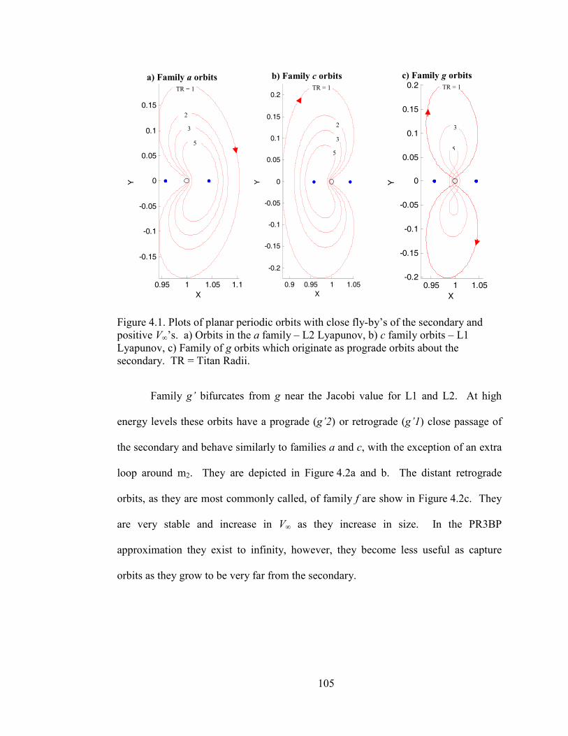
105
0.95 1 1.05 1.1
-0.15
-0.1
-0.05
0
0.05
0.1
0.15
X
Y
0.9 0.95 1 1.05
-0.2
-0.15
-0.1
-0.05
0
0.05
0.1
0.15
0.2
X
Y
0.95 1 1.05-0.2
-0.15
-0.1
-0.05
0
0.05
0.1
0.15
0.2
X
Y
Figure 4.1. Plots of planar periodic orbits with close fly-by’s of the secondary and positive V∞’s. a) Orbits in the a family – L2 Lyapunov, b) c family orbits – L1 Lyapunov, c) Family of g orbits which originate as prograde orbits about the secondary. TR = Titan Radii.
Family g’ bifurcates from g near the Jacobi value for L1 and L2. At high
energy levels these orbits have a prograde (g’2) or retrograde (g’1) close passage of
the secondary and behave similarly to families a and c, with the exception of an extra
loop around m2. They are depicted in Figure 4.2a and b. The distant retrograde
orbits, as they are most commonly called, of family f are show in Figure 4.2c. They
are very stable and increase in V∞ as they increase in size. In the PR3BP
approximation they exist to infinity, however, they become less useful as capture
orbits as they grow to be very far from the secondary.
TR = 1 TR = 1 TR = 1
3
2
5
2
3
5
3
5
a) Family a orbits b) Family c orbits c) Family g orbits
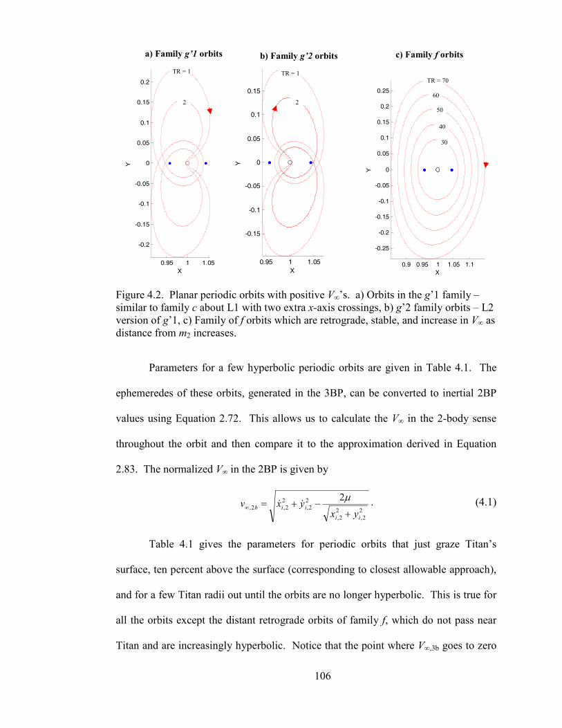
106
0.95 1 1.05
-0.2
-0.15
-0.1
-0.05
0
0.05
0.1
0.15
0.2
X
Y
0.95 1 1.05
-0.15
-0.1
-0.05
0
0.05
0.1
0.15
X
Y
0.9 0.95 1 1.05 1.1
-0.25
-0.2
-0.15
-0.1
-0.05
0
0.05
0.1
0.15
0.2
0.25
X
Y
Figure 4.2. Planar periodic orbits with positive V∞’s. a) Orbits in the g’1 family – similar to family c about L1 with two extra x-axis crossings, b) g’2 family orbits – L2 version of g’1, c) Family of f orbits which are retrograde, stable, and increase in V∞ as distance from m2 increases.
Parameters for a few hyperbolic periodic orbits are given in Table 4.1. The
ephemeredes of these orbits, generated in the 3BP, can be converted to inertial 2BP
values using Equation 2.72. This allows us to calculate the V∞ in the 2-body sense
throughout the orbit and then compare it to the approximation derived in Equation
2.83. The normalized V∞ in the 2BP is given by
2
2,
2
2,
2
2,
2
2,2,
2
ii
iib
yxyxv
+−+=∞
µ&& . (4.1)
Table 4.1 gives the parameters for periodic orbits that just graze Titan’s
surface, ten percent above the surface (corresponding to closest allowable approach),
and for a few Titan radii out until the orbits are no longer hyperbolic. This is true for
all the orbits except the distant retrograde orbits of family f, which do not pass near
Titan and are increasingly hyperbolic. Notice that the point where V∞,3b goes to zero
a) Family g’1 orbits b) Family g’2 orbits c) Family f orbits
TR = 1 TR = 1 TR = 70
2 2 60
50
40
30
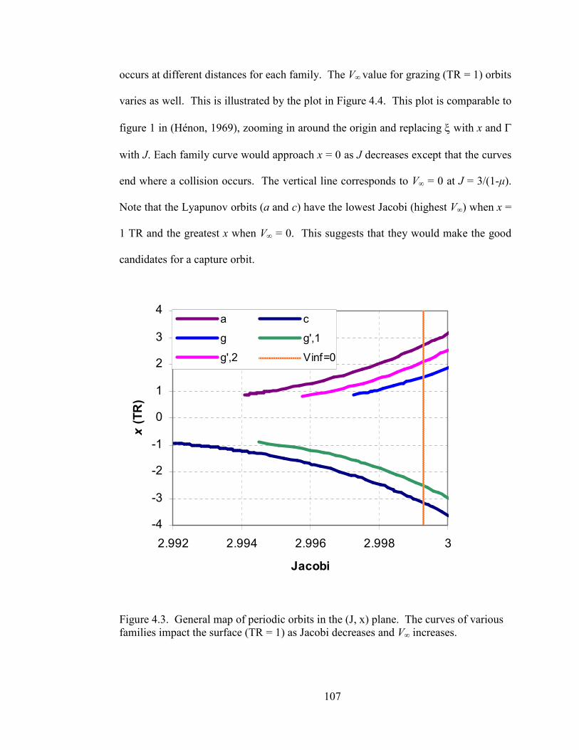
107
occurs at different distances for each family. The V∞ value for grazing (TR = 1) orbits
varies as well. This is illustrated by the plot in Figure 4.4. This plot is comparable to
figure 1 in (Hénon, 1969), zooming in around the origin and replacing ξ with x and Γ
with J. Each family curve would approach x = 0 as J decreases except that the curves
end where a collision occurs. The vertical line corresponds to V∞ = 0 at J = 3/(1-µ).
Note that the Lyapunov orbits (a and c) have the lowest Jacobi (highest V∞) when x =
1 TR and the greatest x when V∞ = 0. This suggests that they would make the good
candidates for a capture orbit.
-4
-3
-2
-1
0
1
2
3
4
2.992 2.994 2.996 2.998 3
Jacobi
x (
TR
)
a c
g g',1
g',2 Vinf=0
Figure 4.3. General map of periodic orbits in the (J, x) plane. The curves of various families impact the surface (TR = 1) as Jacobi decreases and V∞ increases.
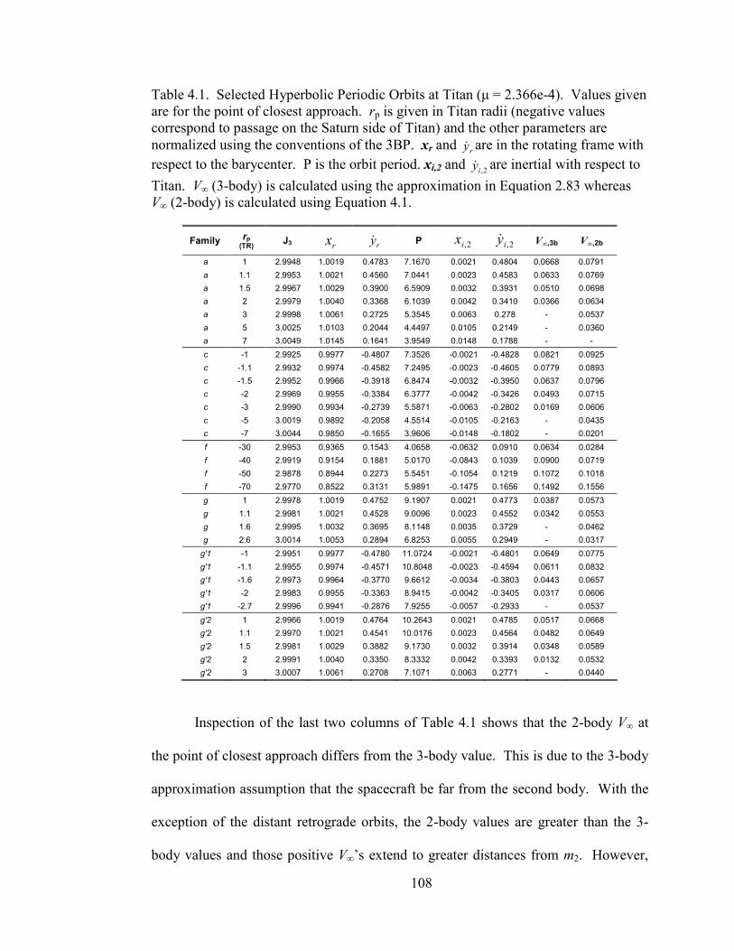
108
Table 4.1. Selected Hyperbolic Periodic Orbits at Titan (µ = 2.366e-4). Values given are for the point of closest approach. rp is given in Titan radii (negative values correspond to passage on the Saturn side of Titan) and the other parameters are
normalized using the conventions of the 3BP. xr and ry& are in the rotating frame with
respect to the barycenter. P is the orbit period. xi,2 and 2,iy& are inertial with respect to
Titan. V∞ (3-body) is calculated using the approximation in Equation 2.83 whereas V∞ (2-body) is calculated using Equation 4.1.
Family rp
(TR) J3 rx ry& P 2,ix 2,iy& V∞,3b V∞,2b
a 1 2.9948 1.0019 0.4783 7.1670 0.0021 0.4804 0.0668 0.0791
a 1.1 2.9953 1.0021 0.4560 7.0441 0.0023 0.4583 0.0633 0.0769
a 1.5 2.9967 1.0029 0.3900 6.5909 0.0032 0.3931 0.0510 0.0698
a 2 2.9979 1.0040 0.3368 6.1039 0.0042 0.3410 0.0366 0.0634
a 3 2.9998 1.0061 0.2725 5.3545 0.0063 0.278 - 0.0537
a 5 3.0025 1.0103 0.2044 4.4497 0.0105 0.2149 - 0.0360
a 7 3.0049 1.0145 0.1641 3.9549 0.0148 0.1788 - -
c -1 2.9925 0.9977 -0.4807 7.3526 -0.0021 -0.4828 0.0821 0.0925
c -1.1 2.9932 0.9974 -0.4582 7.2495 -0.0023 -0.4605 0.0779 0.0893
c -1.5 2.9952 0.9966 -0.3918 6.8474 -0.0032 -0.3950 0.0637 0.0796
c -2 2.9969 0.9955 -0.3384 6.3777 -0.0042 -0.3426 0.0493 0.0715
c -3 2.9990 0.9934 -0.2739 5.5871 -0.0063 -0.2802 0.0169 0.0606
c -5 3.0019 0.9892 -0.2058 4.5514 -0.0105 -0.2163 - 0.0435
c -7 3.0044 0.9850 -0.1655 3.9606 -0.0148 -0.1802 - 0.0201
f -30 2.9953 0.9365 0.1543 4.0658 -0.0632 0.0910 0.0634 0.0284
f -40 2.9919 0.9154 0.1881 5.0170 -0.0843 0.1039 0.0900 0.0719
f -50 2.9878 0.8944 0.2273 5.5451 -0.1054 0.1219 0.1072 0.1018
f -70 2.9770 0.8522 0.3131 5.9891 -0.1475 0.1656 0.1492 0.1556
g 1 2.9978 1.0019 0.4752 9.1907 0.0021 0.4773 0.0387 0.0573
g 1.1 2.9981 1.0021 0.4528 9.0096 0.0023 0.4552 0.0342 0.0553
g 1.6 2.9995 1.0032 0.3695 8.1148 0.0035 0.3729 - 0.0462
g 2.6 3.0014 1.0053 0.2894 6.8253 0.0055 0.2949 - 0.0317
g'1 -1 2.9951 0.9977 -0.4780 11.0724 -0.0021 -0.4801 0.0649 0.0775
g'1 -1.1 2.9955 0.9974 -0.4571 10.8048 -0.0023 -0.4594 0.0611 0.0832
g'1 -1.6 2.9973 0.9964 -0.3770 9.6612 -0.0034 -0.3803 0.0443 0.0657
g'1 -2 2.9983 0.9955 -0.3363 8.9415 -0.0042 -0.3405 0.0317 0.0606
g'1 -2.7 2.9996 0.9941 -0.2876 7.9255 -0.0057 -0.2933 - 0.0537
g'2 1 2.9966 1.0019 0.4764 10.2643 0.0021 0.4785 0.0517 0.0668
g'2 1.1 2.9970 1.0021 0.4541 10.0176 0.0023 0.4564 0.0482 0.0649
g'2 1.5 2.9981 1.0029 0.3882 9.1730 0.0032 0.3914 0.0348 0.0589
g'2 2 2.9991 1.0040 0.3350 8.3332 0.0042 0.3393 0.0132 0.0532
g'2 3 3.0007 1.0061 0.2708 7.1071 0.0063 0.2771 - 0.0440
Inspection of the last two columns of Table 4.1 shows that the 2-body V∞ at
the point of closest approach differs from the 3-body value. This is due to the 3-body
approximation assumption that the spacecraft be far from the second body. With the
exception of the distant retrograde orbits, the 2-body values are greater than the 3-
body values and those positive V∞’s extend to greater distances from m2. However,

109
this relationship does not hold true over the entire orbit. If the instantaneous V∞,2b is
calculated over the whole 3-body orbit, we can see that it varies widely. Figure 4.4
shows the V∞ values over three a-type orbits with rp = 1.1, 1.6, and 2 TR. For lower
energy orbits, the V∞,2b curve actually goes to zero for those times that the spacecraft
is far from the secondary, indicating that the periodic orbit is hyperbolic near closest
0 0.2 0.4 0.6 0.8 10
0.02
0.04
0.06
0.08
0.1
0.12
Orbit Phase
V∞∞ ∞∞ (
VU
)
2-Body
3-Body
Figure 4.4. Instantaneous V∞ values over one orbital period for family a orbits with rp = 1.1 TR(blue), 1.5 TR(red), and 2 TR(green). Phase = 0 corresponds to the point of closest approach.
approach and gravitationally bound elsewhere. The fact that V∞,2b > V∞,3b at t = 0 is
true for all orbits (excluding f) where V∞,3b > 0, further bolstering the rationale to use
hyperbolic periodic orbits as a capture mechanism.
TR =
1.1
2
1.5
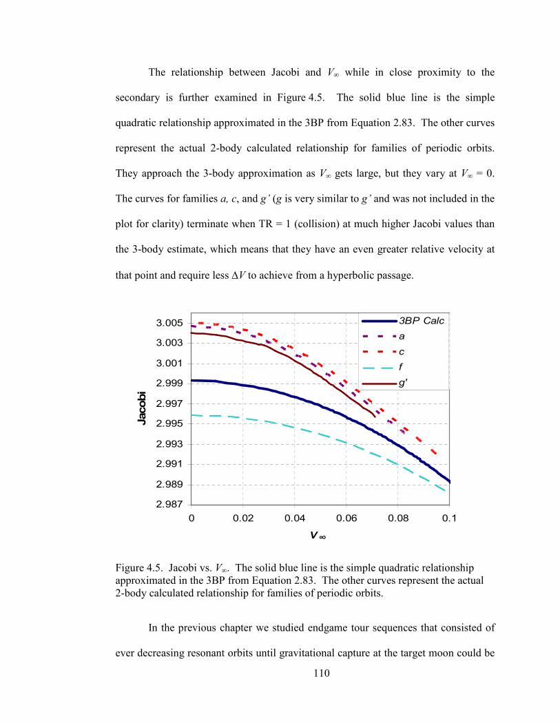
110
The relationship between Jacobi and V∞ while in close proximity to the
secondary is further examined in Figure 4.5. The solid blue line is the simple
quadratic relationship approximated in the 3BP from Equation 2.83. The other curves
represent the actual 2-body calculated relationship for families of periodic orbits.
They approach the 3-body approximation as V∞ gets large, but they vary at V∞ = 0.
The curves for families a, c, and g’ (g is very similar to g’ and was not included in the
plot for clarity) terminate when TR = 1 (collision) at much higher Jacobi values than
the 3-body estimate, which means that they have an even greater relative velocity at
that point and require less ∆V to achieve from a hyperbolic passage.
2.987
2.989
2.991
2.993
2.995
2.997
2.999
3.001
3.003
3.005
0 0.02 0.04 0.06 0.08 0.1
V∞
Jacobi
3BP Calc
a
c
f
g'
Figure 4.5. Jacobi vs. V∞. The solid blue line is the simple quadratic relationship approximated in the 3BP from Equation 2.83. The other curves represent the actual 2-body calculated relationship for families of periodic orbits.
In the previous chapter we studied endgame tour sequences that consisted of
ever decreasing resonant orbits until gravitational capture at the target moon could be
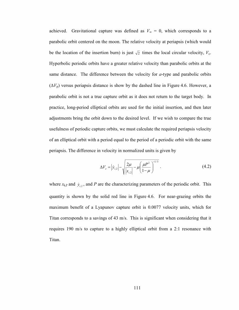
111
achieved. Gravitational capture was defined as V∞ = 0, which corresponds to a
parabolic orbit centered on the moon. The relative velocity at periapsis (which would
be the location of the insertion burn) is just 2 times the local circular velocity, Vc.
Hyperbolic periodic orbits have a greater relative velocity than parabolic orbits at the
same distance. The difference between the velocity for a-type and parabolic orbits
(∆Vp) versus periapsis distance is show by the dashed line in Figure 4.6. However, a
parabolic orbit is not a true capture orbit as it does not return to the target body. In
practice, long-period elliptical orbits are used for the initial insertion, and then later
adjustments bring the orbit down to the desired level. If we wish to compare the true
usefulness of periodic capture orbits, we must calculate the required periapsis velocity
of an elliptical orbit with a period equal to the period of a periodic orbit with the same
periapsis. The difference in velocity in normalized units is given by
3/1
2
2,
2,1
2−
−−−=∆
µµ
µµ P
xyV
i
ie& . (4.2)
where xi,2 and 2,iy& , and P are the characterizing parameters of the periodic orbit. This
quantity is shown by the solid red line in Figure 4.6. For near-grazing orbits the
maximum benefit of a Lyapunov capture orbit is 0.0077 velocity units, which for
Titan corresponds to a savings of 43 m/s. This is significant when considering that it
requires 190 m/s to capture to a highly elliptical orbit from a 2:1 resonance with
Titan.
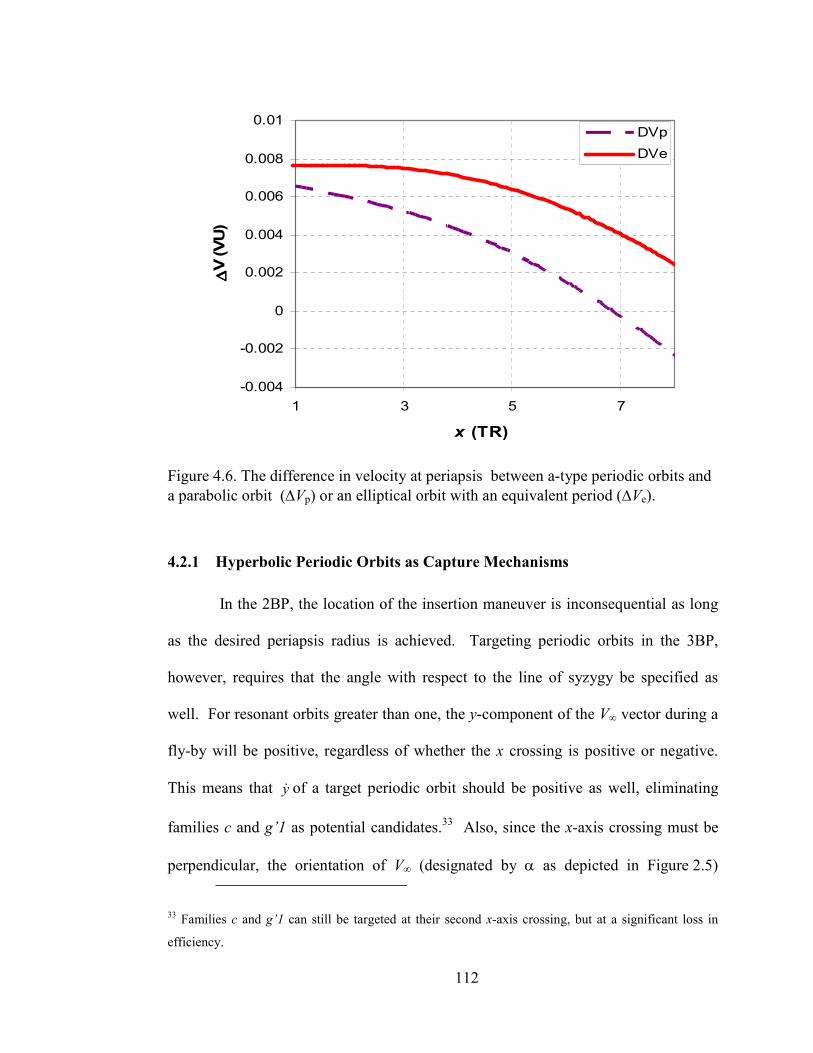
112
-0.004
-0.002
0
0.002
0.004
0.006
0.008
0.01
1 3 5 7
x (TR)
∆∆ ∆∆V
(V
U)
DVp
DVe
Figure 4.6. The difference in velocity at periapsis between a-type periodic orbits and
a parabolic orbit (∆Vp) or an elliptical orbit with an equivalent period (∆Ve).
4.2.1 Hyperbolic Periodic Orbits as Capture Mechanisms
In the 2BP, the location of the insertion maneuver is inconsequential as long
as the desired periapsis radius is achieved. Targeting periodic orbits in the 3BP,
however, requires that the angle with respect to the line of syzygy be specified as
well. For resonant orbits greater than one, the y-component of the V∞ vector during a
fly-by will be positive, regardless of whether the x crossing is positive or negative.
This means that y& of a target periodic orbit should be positive as well, eliminating
families c and g’1 as potential candidates.33 Also, since the x-axis crossing must be
perpendicular, the orientation of V∞ (designated by α as depicted in Figure 2.5)
33 Families c and g’1 can still be targeted at their second x-axis crossing, but at a significant loss in
efficiency.
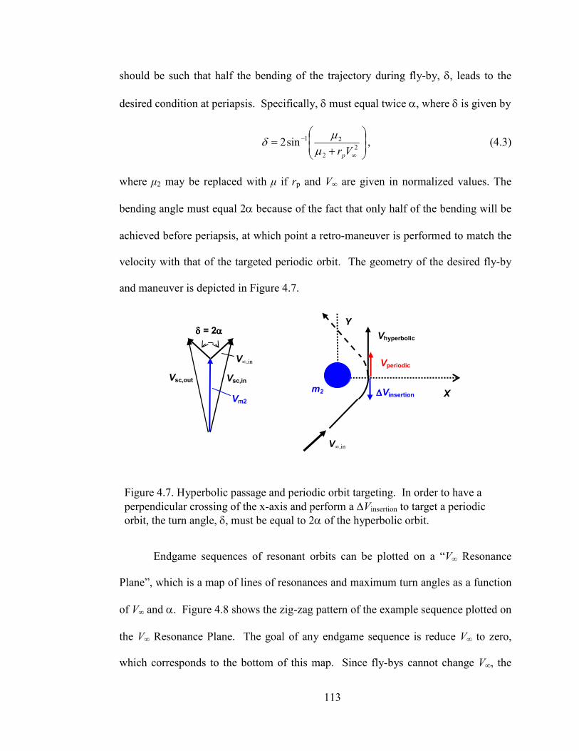
113
should be such that half the bending of the trajectory during fly-by, δ, leads to the
desired condition at periapsis. Specifically, δ must equal twice α, where δ is given by
+=
∞
−2
2
21sin2Vrpµ
µδ , (4.3)
where µ2 may be replaced with µ if rp and V∞ are given in normalized values. The
bending angle must equal 2α because of the fact that only half of the bending will be
achieved before periapsis, at which point a retro-maneuver is performed to match the
velocity with that of the targeted periodic orbit. The geometry of the desired fly-by
and maneuver is depicted in Figure 4.7.
Figure 4.7. Hyperbolic passage and periodic orbit targeting. In order to have a
perpendicular crossing of the x-axis and perform a ∆Vinsertion to target a periodic
orbit, the turn angle, δ, must be equal to 2α of the hyperbolic orbit.
Endgame sequences of resonant orbits can be plotted on a “V∞ Resonance
Plane”, which is a map of lines of resonances and maximum turn angles as a function
of V∞ and α. Figure 4.8 shows the zig-zag pattern of the example sequence plotted on
the V∞ Resonance Plane. The goal of any endgame sequence is reduce V∞ to zero,
which corresponds to the bottom of this map. Since fly-bys cannot change V∞, the
X
Vhyperbolic
m2
Vperiodic
∆∆∆∆Vinsertion
V∞,in
Y
Vm2
Vsc,in Vsc,out
V∞,in
δδδδ = 2αααα
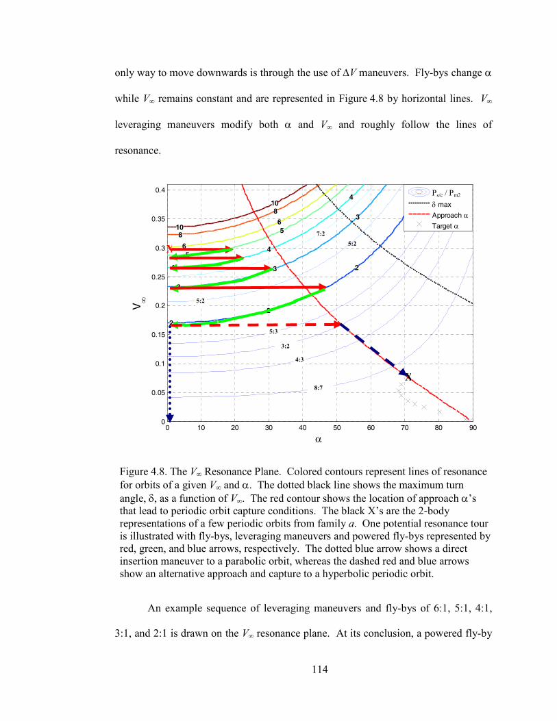
114
only way to move downwards is through the use of ∆V maneuvers. Fly-bys change α
while V∞ remains constant and are represented in Figure 4.8 by horizontal lines. V∞
leveraging maneuvers modify both α and V∞ and roughly follow the lines of
resonance.
0 10 20 30 40 50 60 70 80 900
0.05
0.1
0.15
0.2
0.25
0.3
0.35
0.42
2
2
2
3
3
3
4
4
4
5
5
6
6
8
8
10
10
α
V∞
T
sc / T
ga
δ max
Approach αTarget α
Figure 4.8. The V∞ Resonance Plane. Colored contours represent lines of resonance
for orbits of a given V∞ and α. The dotted black line shows the maximum turn
angle, δ, as a function of V∞. The red contour shows the location of approach α’s that lead to periodic orbit capture conditions. The black X’s are the 2-body representations of a few periodic orbits from family a. One potential resonance tour is illustrated with fly-bys, leveraging maneuvers and powered fly-bys represented by red, green, and blue arrows, respectively. The dotted blue arrow shows a direct insertion maneuver to a parabolic orbit, whereas the dashed red and blue arrows show an alternative approach and capture to a hyperbolic periodic orbit.
An example sequence of leveraging maneuvers and fly-bys of 6:1, 5:1, 4:1,
3:1, and 2:1 is drawn on the V∞ resonance plane. At its conclusion, a powered fly-by
X
X
5:2
7:2
5:2
5:3
3:2
4:3
8:7
Ps/c / Pm2
115
maneuver is performed to reduce V∞ to zero. This sequence requires 0.046 VU (258
m/s @ Titan) in ∆V, of which 0.033 (190 m/s) are needed for the final maneuver, and
88 TU (223 days) to perform. This result can be compared to a direct insertion
maneuver from the 6:1 resonance (V∞ = 0.3048) to V∞ = 0, which requires 0.097 VU
(540 m/s). The added flight time of the resonance tour buys over 50% in ∆V savings.
There are hundreds of possible resonance sequences that result in up to 60%
∆V savings for only a modest increase in total flight time (Woolley and Scheeres,
2010). The problem is that the final insertion maneuver in each sequence typically
uses around 75% of the total sequence ∆V requirement. If a hyperbolic periodic orbit
is targeted at the end of the sequence then about 0.007 VU (~40 m/s) can be saved.
This is about 25% of the final insertion maneuver, or an additional 8% savings versus
the direct insertion approach.
The sequence plotted on Figure 4.8 concludes at V∞ = 0, shown by the
vertical, blue dotted arrow. An alternate conclusion to a periodic orbit is shown by
the red and blue dashed arrows. The red one represents a fly-by designed to set up
the final insertion approach geometry by targeting the α = ½δmax line depicted by the
red contour. Halfway through the subsequent fly-by, an insertion maneuver matches
the velocity to that of the periodic orbit and capture occurs. This is represented by the
blue dashed arrow that terminates at the bold X, which still has a positive V∞.
The δmax and approach α lines are calculated for a specific radius of periapsis,
in this case rp = 1.1 TR. Capture can take place at greater distances, but this is
usually at a loss in efficiency, as ∆V maneuvers are most efficient were velocity is the
greatest. The other X’s near the bottom right-hand corner of the plot represent the
116
target conditions for other periodic orbits with increasing periapses. They are each the
termination point of a corresponding approach α line and represent the 2-body
conditions that result in a 3-body “exit” from the V∞ Resonance Plane.
4.3 Conclusion
Periodic orbits in the PR3BP that exist near the secondary and are hyperbolic
in the 2BP are useful as capture mechanisms at planetary moons. We have shown
that most families of simple periodic orbits have increasingly positive V∞’s as their
periapses approach the radius of the target moon. Lyapunov orbits (families a and c)
have the highest V∞ for a given periapsis distance, and family a is the most suitable
for capture from resonance orbits greater than one due to its approach geometry
conditions. Targeting a “hyperbolic periodic” orbit during the final phase of a
leveraging maneuver sequence results in a lower required insertion ∆V, on the order
of 20-25%.
This dissertation explores the limits and usefulness of hyperbolic periodic
orbits and their application to the endgame problem. Orbits were generated using a
single shooting method in the planar restricted problem and integrated into the final
phase of leveraging sequences found in Section 3.6. We showed that using a
hyperbolic periodic orbit to capture to the vicinity of a target moon following an
optimized sequence of leveraging maneuvers and fly-bys yields significant fuel
savings (60-70%) over direct trajectories.
We have only presented simple planar periodic orbits, yet an infinite number
of more complex periodic and quasi-periodic orbits exist. It is unlikely that higher
117
order planar orbits will result in higher V∞’s at the same distances as Lyapunov orbits,
however, they may exhibit properties that are much more desirable from a mission
design standpoint. Depending on a mission’s requirements (∆V, duration, science
objectives, lighting angles, communications, etc.), any of the 3-body periodic orbits
may exhibit both pros and cons for mission optimization. There also exist 3-
dimensional periodic orbits that can be used as efficient capture and transfer
mechanisms for orbiters wishing to achieve low, highly-inclined science orbits about
a planetary moon.
118
5 Discussion
5.1 Overview of Findings
V∞ leveraging is a useful tool in the design of planetary moon endgame
strategies. If applied properly it is possible to significantly reduce the total ∆V
required to send an orbiter to a planetary moon such as Titan. In this dissertation we
present theoretical calculations that show that the total ∆V required can be up to 10
times or more the change in ∆V∞. While the theoretical minima require infinite
durations, they do serve to illustrate a lower bound on the fuel required to place a
spacecraft into a captured orbit. As the V∞ decreases, leveraging maneuvers become
less and less efficient. Below a certain point, it was shown that powered fly-bys
become a more efficient means of V∞ reduction.
In addition, we have developed tools to construct, map, and analyze sequences
of leveraging maneuvers and to compare them to the theoretical minimum. The
reduction in fuel requirements comes at the expense of added flight time. Tens of
thousands of sequences were generated using a Monte-Carlo type simulation and the
total ∆V and TOF pairs were accumulated. By plotting these pairs we were able to
generate a Pareto front of most efficient sequences for a given flight time.
Reducing a 6:1 orbit to V∞ = 0 using a direct burn during fly-by would require
0.097 velocity units, whereas an infinite series of fly-bys and leveraging maneuvers
119
(theoretical minimum) would reduce the total ∆V required to 0.028, a savings of over
70%. Since infinite missions are not possible, it is helpful to the mission designer to
know that it is possible to reduce the total ∆V by 50% with a TOF of only 5-10 time
units. Increasing the mission duration further does not result in significant reductions.
Periodic orbits in the PR3BP that exist near the secondary and are hyperbolic
in the 2BP are useful as capture mechanisms at planetary moons. We have shown
that most families of simple periodic orbits have increasingly positive V∞’s as their
periapses approach the radius of the target moon. Lyapunov orbits (families a and c)
have the highest V∞ for a given periapsis distance, and family a is the most suitable
for capture from resonance orbits greater than one due to its approach geometry
conditions. Targeting a “hyperbolic periodic” orbit during the final phase of a
leveraging maneuver sequence results in a lower required insertion ∆V, on the order
of 20-25%.
5.1.1 Contributions to the Field
The V∞ Sphere and V∞ Plane are useful design tools in that they allow the
designer to quickly see what types of orbits are possible given a set of input
parameters. Post fly-by orbits can be targeted by noting the change of α required on
the V∞ Plane. Sequences of leveraging maneuvers and fly-bys can be plotted as points
on the map.
This dissertation provides a new method for the design and analysis of V∞
leveraging maneuvers – the Lambert solution technique. This allows us to quantify
and optimize these maneuvers with the aide of efficiency contours. This technique
120
frees some of the constraints traditionally placed on leveraging maneuvers (e.g. that
the maneuver take place exactly at apoapsis).
Armed with this tool, we generated tens of thousands of resonance sequences
that are optimized at each leveraging maneuver. The results allow us to analyze the
trends that characterize optimal trajectories. They also provide the mission designer
with a good understanding of the trade off between the reduction of total ∆V and the
increase in total time-of-flight.
The final section of this dissertation explored the relationships between the
two- and three-body problems. This is useful during the capture phase as the
transition to the target moon’s sphere of influence is better understood in the three-
body realm. We showed that hyperbolic periodic orbits do exist and can be more
useful as capture mechanisms than standard two-body orbits. We also provided
common terminology and metrics that allow seamless connection of the capture
portion of a trajectory to the tour sequence and to evaluate its usefulness.
5.1.2 Areas of Future Research
The maneuver sequences detailed in this dissertation are restricted to orbits
confined to the plane of the gravity-assist body and are very theoretical in nature. In
practice planetary tours make use of inclined orbits, fly by other moons, and must
take into account many other factors. Because of this, the more “optimal” tour
sequences generated here are not necessarily what would be used in true mission
design. However, the tools and results are instructive for preliminary analyses and
for understanding the trends that lead to optimal tour design.
121
We have only presented simple planar periodic orbits, yet an infinite number
of more complex periodic and quasi-periodic orbits exist. It is unlikely that higher
order planar orbits will result in higher V∞’s at the same distances as Lyapunov orbits,
however, they may exhibit properties that are much more desirable from a mission
design standpoint. Depending on a mission’s requirements (∆V, duration, science
objectives, lighting angles, communications, etc.), any of the 3-body periodic orbits
may exhibit both pros and cons for mission optimization. There also exist 3-
dimensional periodic orbits that can be used as efficient capture and transfer
mechanisms for orbiters wishing to achieve low, highly-inclined science orbits about
a planetary moon.
122
6 Bibliography
Anderson, R.L., Low Thrust Trajectory Design for Resonant Flybys and Captures
Using Invariant Manifolds. PhD, University of Colorado, 2005.
Barrow-Green, J. Poincaré and the Three Body Problem. American Mathematical Society - London Mathematical Society, Providence, Rhode Island, 1997.
Bate, R., D. Mueller, and J. White, Fundamentals of Astrodynamics, New Dover Publications, New York, 1971, pp. 198-233.
Battin, R.H., An Introduction to the Mathematics and Methods of Astrodynamics, AIAA Education Series, AIAA, New York, 1987.
Boutonnet, A., P. d. Pascale, and E. Canalias, “Desing of the Laplace Mission,” Paper IAC-08-C1.6, 59th IAC, Glasgow, Scottland, 2008.
Breakwell, J.V. and J.V. Brown, “The ‘Halo’ Family of 3-Dimensional Periodic Orbits in the Earth-Moon Restricted 3-Body Problem,” Celestial Mechanics, vol. 20, p. 389, 1979.
Brinckerhoff, A.T. and R.P. Russell, “Pathfinding and V∞ Leveraging for Planetary Moon Tour Missions,” AIAA/AAS Space Flight Mechanics Meeting, AAS Paper 09-222, Savannah, Georgia, February 2009.
Campagnola, S. and R.P. Russell, “Endgame Problem Part 1: V∞-Leveraging Technique and the Leveraging Graph,” Journal of Guidance, Control, and
Dynamics, Vol. 33, No. 2, pp. 463-475, March-April 2010a.
Campagnola, S. and R.P. Russell, “Endgame Problem Part 2: Multi-body Technique and the Tisserand-Poincaré Graph,” Journal of Guidance, Control, and
Dynamics, Vol. 33, No. 2, pp. 476-486, March-April 2010b.
Campagnola, S., N.J. Strange, and R.P. Russell, “A Fast Tour Design Method Using Non-Tangent V-Infinity Leveraging Transfers,” AAS/AIAA Spaceflight
Mechanics Meeting, AAS Paper 10-164, San Diego, CA, February 2010c.
123
Casalino, L., G. Colasurdo, and D. Pastrone, “Optimization of Delta-V Earth-Gravity-Assist Trajectories,” Journal of Guidance, Control, and Dynamics, Vol. 21, No. 6, November 1998.
Chobotov, V., “Orbital Mechanics”, AIAA Education Series, 1991.
Clark, K. C., R. Greeley, R. Pappalardo, and C. Jones, “2007 Europa Explorer Mission Study: Final Report,” Task Order #NMO710851, JPL D-41283, November 1, 2007.
Colasurdo, G., L. Casalino, and E. Fantino, “Minimum-fuel Escape from Two-Body Sun-Earth System.” Journal of Guidance, Control, and Dynamics, Vol. 22, No. 5, September 1999.
Curtis, H. D., Orbital Mechanics for Engineering Students, Elsevier, 2005.
Danby, J.M.A., Fundamentals of Celestial Mechanics, Willmann-Bell, Inc., Richmond, VA, 1992.
Darwin, G. H., “Periodic Orbits,” Acta Mathematica, Vol. 21, pp. 99–242, 1897.
Darwin, G. H., “Periodic Orbits,” Scientific Papers, Vol. 4, Cambridge University Press, Cambridge, Mass., 1911.
Davis, K. E., Locally Optimal Transfer Trajectories Between Libration Point Orbits
Using Invariant Manifolds, PhD, University of Colorado, 2009.
Demeyer, J. and P. Gurfil, "Transfer to Small Distant Retrograde Orbits," in New
Trends in Astrodynamics and Applications III, E. Belbruno, Ed., vol. 886, pp. 20-31, Princeton, New Jersey 2007.
Edwards, W. et al., “Titan Explorer: The Next Step in the Exploration of a Mysterious World,” Final Report for NASA Vision Mission Study, NRA-03-OSS-01, Presented at the Outer Planets Assessment Group, October 6-7, 2005.
Euler, L., Theoria Motuum Planetarum et Cometarum, Berlin, 1744.
Farquhar, R. W. “The Flight of ISEE-3/ICE: Origins, Mission History, and a Legacy.” AIAA Paper 98-4464, AIAA/AAS Astrodynamics Specialist
Conference and Exhibit, Boston, Massachusetts, August 1998.
Gomez, G., M. Lara, and R. Russell, “A Dynamical Systems Approach to the Design of the Science Orbit Around Europa,” ISTS, 2006.
Heaton, A.F., N. J. Strange, J. M. Longuski, and E. P. Bonfiglio, “Automated Design of the Europa Orbiter Tour,” AIAA Paper 2000-4034, 2000.
124
Hénon, M., “Exploration Numérique du Probléme des Trois Corps, I. Masses égales, Orbites Périodiques,” Ann. d'Astrophys. Vol. 28, pp. 499-511, 1965a.
Hénon, M., “Exploration Numérique du Probléme des Trois Corps, II. Masses égales, stabilité des orbites périodiques,” Ann. d'Astrophys. Vol. 28, pp. 992-1000, 1965b.
Hénon, M., “Exploration Numérique du Probléme des Trois Corps, III. Masses Egales, Orbites Non Périodiques,” Bull. Astron., Volume 1(1), pp. 57–80, 1966a.
Hénon, M., “Exploration Numérique du Probléme des Trois Corps, IV. Masses Egales, Orbites Non Périodiques,” Bull. Astron., Volume 1(2), pp. 49–66, 1966b.
Hénon, M., “Generating Families in the Restricted Three-Body Problem,” Lecture
Notes in Physics, Vol. 52, Springer, Berlin, 1997.
Hénon, M., “New Families of Periodic Orbits in Hill’s Problem of Three Bodies,” Celestial Mechanics and Dynamical Astronomy, Vol. 85, pp. 223-246, 2003.
Hénon, M., “Numerical Exploration of the Restricted Problem. VI. Hill's Case: Non-Periodic Orbits.” Astronomy and Astrophysics. Vol. 1, pp. 24-36, 1970.
Hénon, M., “Numerical Exploration of the Restricted Problem.V. Hill’s Case: Periodic Orbits and Their Stability.” Astronomy and Astrophysics, Vol. 1, pp. 223–238, 1969.
Hill, G.W., “Researches in the Lunar Theory,” American Journal of Mathematics, Vol. 1, No. 1, 1878, pp. 5–26.
Hollenbeck, G.R., “New Flight Techniques for Outer Planet Missions,” AAS/AIAA
Astrodynamics Specialist Conference, AAS Paper 75-087. July 1975.
Howell, K.C., “Three-Dimensional, Periodic, ‘Halo’ Orbits,” Celestial Mechanics, vol. 32, pp. 53-71, 1984.
Johannesen, J.L. and L.A. D'Amario, “Europa Orbiter Mission Trajectory Design,” AAS/AIAA Astrodynamics Specialist Conference, AAS Paper 99-360, Girdwood, Alaska, August 1999.
Lagrange, J., “Essai sur le probléme des trois corps,” Gallica, Volume 6, pp. 272–292, 1867-1892.
125
Lam, T. and G. J. Whiffen, "Exploration of Distant Retrograde Orbits around Europa," AAS/AIAA Space Flight Mechanics Meeting, AAS Paper 05-110, January 2005.
Lyapunov, A. M., “The General Problem of the Stability of Motion,” Comm. Soc.
Math. Kharkow, 1892.
Nakamiya, M., D.J. Scheeres, H. Yamakawa, and M. Yoshikawa, "Analysis of Capture Trajectories into Periodic Orbits about Libration Points," AAS/AIAA
Spaceflight Mechanics Meeting, AAS Paper 07-228, Sedona, Arizona, 2007.
Newton, I., Philosophiae Naturalis Principia Mathematica, Londoni, 1687.
Poincaré, H., “Sur le probléme des trois corps et les équations de la dynamique,” Acta
Math., Volume 13,, pp. 1–27, 1890.
Poincaré, H., New Methods of Celestial Mechanics, 1. Periodic and Asymptotic
Solutions, edited by F. Goroff, D. L., American Institute of Physics, USA, 1993.
Prussing, J.E. and B.A. Conway, Orbital Mechanics, Oxford University Press, 1993.
Ross, S.D. and D.J. Scheeres, “Multiple Gravity Assists, Capture, and Escape in the Restricted Three-Body Problem,”
SIAM Journal on Applied Dynamical
Systems, Vol. 6, No. 3, pp. 576-596, 2007a.
Ross, S.D. and P. Grover, “Fuel-optimal Trajectories in a Planet-Moon Environment using Multiple Gravity Assists,” International Symposium on Space Flight
Dynamics, 2007b.
Russell, R.P. and T. Lam, “Designing Capture Trajectories to Unstable Periodic Orbits Around Europa,” AAS/AIAA Space Flight Mechanics Meeting, AAS Paper 06-189, Tampa, Florida, 2006.
Russell, R.P., "Global Search for Planar and Three-Dimensional Periodic Orbits Near Europa," AAS/AIAA Astrodynamics Specialist Conference, AAS Paper 05-290, Lake Tahoe, California, August 2005.
Schaub, H.P. and J.L. Junkins, Analytical Mechanics of Space Sytems, AIAA Education Series, AIAA, Virginia, 2003.
Scheeres, D.J. and M.D. Guman, "Stability Analysis of the Europa Orbiter," Spaceflight Mechanics 2000, Part II, Advances in the Astronautical Sciences
Series, vol. 105, pp. 855-868. Univelt, 2000.
126
Scheeres, D.J., M.D. Guman, and B. F. Villac, “Stability Analysis of Planetary Satellite Orbiters: Application to the Europa Orbiter,” Journal of Guidance,
Control, and Dynamics, vol. 24, no. 4, pp. 778–787, 2001.
Sims, J.A. and J.M. Longuski, “Analysis of V-infinity Leveraging for Interplanetary Missions,” AIAA/AAS Astrodynamics Conference, AAS Paper 94-3769, Scottsdale, AZ, 1994.
Sims, J.A., J.M. Longuski, and A.J. Staugler, “V∞ Leveraging for Interplanetary Missions: Multiple-Revolution Orbit Techniques,” Journal of Guidance
Control and Dynamics, Vol. 20, No. 3, pp. 409-415, 1997.
Strange, N. J. and J. M. Longuski, "Graphical Method for Gravity-Assist Trajectory Design," Journal of Spacecraft and Rockets, vol. 39, no. 1, pp. 9-16, 2002.
Strange, N.J., R. Russell, and B. Buffington, “Mapping the V∞ Globe,” AIAA/AAS
Space Flight Mechanics Meeting, AAS Paper 07-277, 2007.
Strange, N.J., S. Campagnola, and R. Russell, "Leveraging Flybys of Low Mass Moons to Enable an Enceladus Orbiter," AAS/AIAA Astrodynamics Specialist
Conference, AAS Paper 09-435, August 2009a.
Strange, N.J., T.R. Spilker, D.F. Landau, T. Lam, D.T. Lyons, and J.J. Guzman, “Mission Design for the Titan Saturn System Mission Concept," AAS/AIAA
Astrodynamics Conference, AAS Paper 09-356, Pittsburgh, PA, Aug. 2009b.
Strömgren, E., “Connaissance actuelle des orbites dans le probléme des trios corps,” Bulletin Astronomica. Vol. 9, No. 87, 1935.
Sundman, K., “Nouvelle Recherches sur le Probléme des Trois Corps,” Acta
Societatis Scientiarum Fennicae, Volume 35, 1909.
Sweetser, T.H., “Jacobi's Integral and Delta-V-Earth-Gravity-Assist Trajectories,” AAS/AIAA Astrodynamics Specialist Conference, AAS Paper 93-635, Victoria, BC, Canada, August 1993.
Sweetser, T.H., R. Maddock, J. Johannesen, J. Bell, P. A. Penzo, A. Wolf, S. N. Williams, S. Matousek, and S. Weinstein, "Trajectory Design for a Europa Orbiter Mission: A Plethora of Astrodynamic Challenges," Advances in the
Astronautical Sciences, vol. 95, pp. 901-920, 1997.
Szebehely, V., Theory of Orbits. The Restricted Problem of Three Bodies, Academic Press, New York, 1967.
Tisserand, F.F, Traite’ de Mechanique Celeste, Vol. 4. Gauthier-Villars et fils, 1896.
127
Uphoff, C., P. H. Roberts, and L. D. Friedman, “Orbit Design Concepts for Jupiter Orbiter Missions,” Journal of Spacecraft and Rockets, Vol. 13, No. 6, 1976, pp. 348-355.
Vallado, D.A. Fundamentals of Astrodynamics and Applications, Space Technology Library, Microcosm Press, El Segundo, California, 2001.
Villac, B. F. and D. J. Scheeres, "Escaping trajectories in the Hill Three Body Problem and Applications," Journal of Guidance, Control, and Dynamics, vol. 26, no. 2, pp. 224-232, 2003.
Villac, B. F., "Dynamics in the Hill Problem with Applications to Spacecraft Maneuvers," PhD, University of Michigan, 2003.
Wertz, J., Mission Geometry; Orbit and Constellation Design and Management, Space Technology Library, Microcosm Press, El Segundo, California, 2001.
Wiesel, W. E.. Modern Astrodynamics. Aphelion Press, Beavercreek, Ohio, 2004.
Woolley, R.C. and D.J. Scheeres, “Hyperbolic Periodic Orbits in the Three-Body Problem and Their Application to Orbital Capture,” AAS George H. Born Symposium, Boulder, CO, May 13-14, 2010.
Woolley, R.C. and D.J. Scheeres, “Optimal Pathways for Sequences of V-infinity Leveraging Maneuevers,” AAS/AIAA Spaceflight Mechanics Meeting, AAS Paper 10-219, San Diego, CA, February 2010.
Woolley, R.C. and D.J. Scheeres, “Shrinking the V-infinity Sphere: Endgame Strategies for Planetary Moon Orbiters,” AAS/AIAA Astrodynamics Specialist
Conference, AAS Paper 09-377, Pittsburgh, Pennsylvania, August 2009.
128
7 Appendix A: Nomenclature
δ Turn angle of the V∞ vector during a fly-by
ω Angular velocity of secondary body about the primary
τ One time unit, defined by 1/ω
γ Flight path angle between Vga and Vsc
Γ Hénon’s notation for Jacobi constant in Hill’s Problem
δmax The maximum turn angle of a fly-by when rmin is used
a, e, i Semimajor axis, eccentricity, and inclination of an orbit
E Specific mechanical energy (or Eccentric anomaly in 2.1.3)
G Universal gravitation constant
h Angular momentum
J3b, JH Jacobi constant expressed in the 3BP or Hill’s problem, respectively
k Integer constant
K Number of m2 orbit revolutions during leveraging maneuver
l Length unit in Hill’s problem
L Number of spacecraft orbit revolutions during leveraging maneuver
L1, L2 Referring to the 1st and 2nd collinear Lagrangian or Libration points
LU,TU,VU Abbrev. for normalized Length Unit, Time Unit, and Velocity Unit
M Spacecraft orbit revolution number on which the ∆V is applied
129
m1, m2, m3 Referring to the primary, secondary, or spacecraft, respectively
p Semi-parameter
P, Psc, Pga Period of the spacecraft/gravity-assist body
R Distance between the primary, m1, and secondary, m2.
r, r1, r2 Distance from the barycenter, primary, or secondary, respectively
rc Circular radius of final orbit
rga, aga Radius and semimajor axis of the gravity-assist body, which are
equivalent
rmin Minimum allowable fly-by radius of the gravity-assist body
rp Radius of closest approach to the gravity-assist body
rSOI Radius of a body’s sphere-of-influence
S, C, A Universal variables
S, s State vector
Si, Sr Inertial or rotational state vector, respectively
T, Td Non-dimensional and dimensional Tisserand’s Parameter, respectively
TR Periapsis distance equal to one Titan radius
U Augmented effective gravitational potential energy
V∞ Hyperbolic excess velocity of the spacecraft with respect to m2
Vc The local circular velocity at rp around m2
Vga Velocity of the gravity-assist body (circular)
Vp S/C Velocity at periapsis during a fly-by
Vsc Spacecraft velocity with respect to the central body
X, Y Spacecraft coordinates in dimensional units
130
x, y Spacecraft coordinates in non-dimensional units
α The angle between V∞ and Vga
Γ Alternative designation of Jacobi constant
∆V The change in velocity during a maneuver
θ True anomaly of reencounter during a leveraging maneuver
λ Eigenvalue (specifically of the Monodromy STM)
µ Reduced mass of the system - m2/(m1+m2)
µ1 , µ2 Gravitational parameter (GM) of the primary (1) and secondary (2)
ν True anomaly
Ω Longitude of ascending node
Ф State Transition Matrix (STM)
131
8 Appendix B: Coordinate Transformations
The state of a spacecraft in the rotating frame is given by
==
=
y
x
y
x
TsT
Y
X
Y
X
S n
dr
n
dr
&
&
&
& (8.1)
where sr is the state in nondimensional units and Tdn is the transformational matrix
=
R
R
R
R
T n
d
ωω000
000
000
000
(8.2)
To transform the state from the rotational (or synodic) frame to the inertial (or
sidereal) frame we must take into account the rotational offset, θ, and the angular rate,
ω = θ& . Here we will assume the offset is zero (see Anderson (2005) for non-zero θ
transformations). Since the Z axes are aligned in both frames we can write
+
−=
=
XY
YX
Y
X
Y
X
Y
X
S
i
i
i
i
i
ωω
&
&
&
& and
+
−=
=
xy
yx
y
x
y
x
y
x
s
i
i
i
i
i
&
&
&
& (8.3)
where the subscript ‘i’ denotes the inertial frame. (A subscript ‘r’ has been omitted
from the rotational quantities for clarity and redundancy). Notice that ω = 1 in the
nondimensional frame. The relations in (2.72) can be reversed:
132
−
+=
ii
ii
i
i
r
XY
YX
Y
X
S
ωω
&
& and
−
+=
ii
ii
i
i
r
xy
yx
y
x
s
&
& (8.4)
Recall that the rotating frame is centered at the barycenter of m1 and m2.
However, most inertial frames are centered on either of the bodies. As such we must
shift the state vectors to the new center.
++
−
+
=
)( 1
1
1,
RXY
YX
Y
RX
S i
ωω
&
&,
−+
−
−
=
)( 2
2
2,
RXY
YX
Y
RX
Si
ωω
&
&
and
++
−
+
=
µ
µ
xy
yx
y
x
si
&
&1, ,
−−+
−
−−
=
)1(
)1(
2,
µ
µ
xy
yx
y
x
si
&
& (8.5)
Where states with the added subscript ‘1’ refer to states centered at the primary and
likewise, ‘2’, for the secondary.
133
9 Appendix C: Notes on Lambert’s Problem
Lambert’s problem is concerned with the determination of an orbit that passes
between two positions within a specified time-of-flight. This classic astrodynamic
problem is also known as the orbital two-point boundary value problem (TPBVP) or
the flyby and rendezvous problems.
9.1 Lambert’s Theorem
The theorem states that the time to traverse a trajectory depends only upon the
length of the semimajor axis a of the transfer trajectory, the sum ri+ rf of the
distances of the initial and final positions relative to a central body, and the length c
of the chord joining these two positions. This relationship can be stated as follows:
tof = tof(ri+ rf, c, a) (9.1)
Using a geometrical approach starting from Kepler’s second law (orbits sweep
out equal areas in equal times), we can derive the following form of Kepler’s
equation
)sin(3
0 EeEa
tt −=−µ
(9.2)
from which we can write
134
)]sin(sin[ 00
3
EEeEEa
t −−−=∆µ
(9.3)
where E is the eccentric anomaly associated with radius r, E0 is the eccentric anomaly
at r0 , and t = 0 when r = r0. At this point we introduce the following trigonometric
sum and difference identities:
2cos
2cos2coscos
2sin
2sin2coscos
2cos
2sin2sinsin
βαβαβα
βαβαβα
βαβαβα
+−=+
+−−=−
+−=−
(9.4)
If we let E = α and E0 = β and substitute the first trig identity into Equation
9.3, we have the following equation:
+−−−=∆
2cos
2sin2 00
0
3 EEe
EEEE
at
µ (9.5)
If we manipulate the elliptic relationships given by
21sin
)(cos
)cos1(
eEay
eEax
Eear
−=
−=
−=
(9.6)
we obtain:
a
c
a
rrE
a
c
a
rrE
221sin
221cos
00
0
+
+−=
−
+−=
(9.7)
Next, we make use of the following three relationships:
135
22
0
2
0
2
00
2
0000
000
2222sin
2sin
2cos1
2sin
2sin
2sin
21
2cos
2cos
=
−+
−=
+−
+−
−=
+−
+−=
+−
a
c
a
yy
a
xxEEEE
EEe
EEEEEE
rrEEEE
(9.8)
along with the trigonometric half angle formulas and several additional substitutions
to derive the time-of-flight form of Lambert’s theorem
[ ])sin(sin 00
3
EEeEEa
t −−−=∆µ
. (9.9)
If we wish to take into account multiple revolutions the time is given by
[ ])sin(sin2 00
3
EEeEEka
t −−−+=∆ πµ
(9.10)
where k is the number of complete revolutions and E is given in radians. The process
of solving Lambert’s theorem for any two position vectors and transfer time is done
using iterations on a universal variable formulation (Vallado, 1997; Prussing and
Conway, 1993).
9.2 Multi-Revolution Solutions to Lambert’s Problem
The universal variables solution to Lambert’s problem, as discussed in Section
2.1.3, only admits hyperbolic and elliptical solutions of less than one full revolution.
This is due to the omission of the 2kπ term of Equation 2.8. The parameter z
increases monotonically with total TOF until z = (2π)2 and TOF ∞. This is shown
in Figure 9.1. When z is negative the solution is hyperbolic and elliptical when it is
greater than zero. However, for long transfer times, it is possible to complete
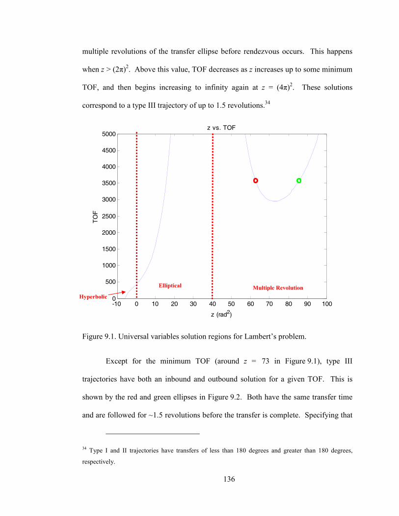
136
multiple revolutions of the transfer ellipse before rendezvous occurs. This happens
when z > (2π)2. Above this value, TOF decreases as z increases up to some minimum
TOF, and then begins increasing to infinity again at z = (4π)2. These solutions
correspond to a type III trajectory of up to 1.5 revolutions.34
-10 0 10 20 30 40 50 60 70 80 90 1000
500
1000
1500
2000
2500
3000
3500
4000
4500
5000z vs. TOF
z (rad2)
TO
F
Figure 9.1. Universal variables solution regions for Lambert’s problem.
Except for the minimum TOF (around z = 73 in Figure 9.1), type III
trajectories have both an inbound and outbound solution for a given TOF. This is
shown by the red and green ellipses in Figure 9.2. Both have the same transfer time
and are followed for ~1.5 revolutions before the transfer is complete. Specifying that
34 Type I and II trajectories have transfers of less than 180 degrees and greater than 180 degrees,
respectively.
Hyperbolic
Multiple Revolution Elliptical
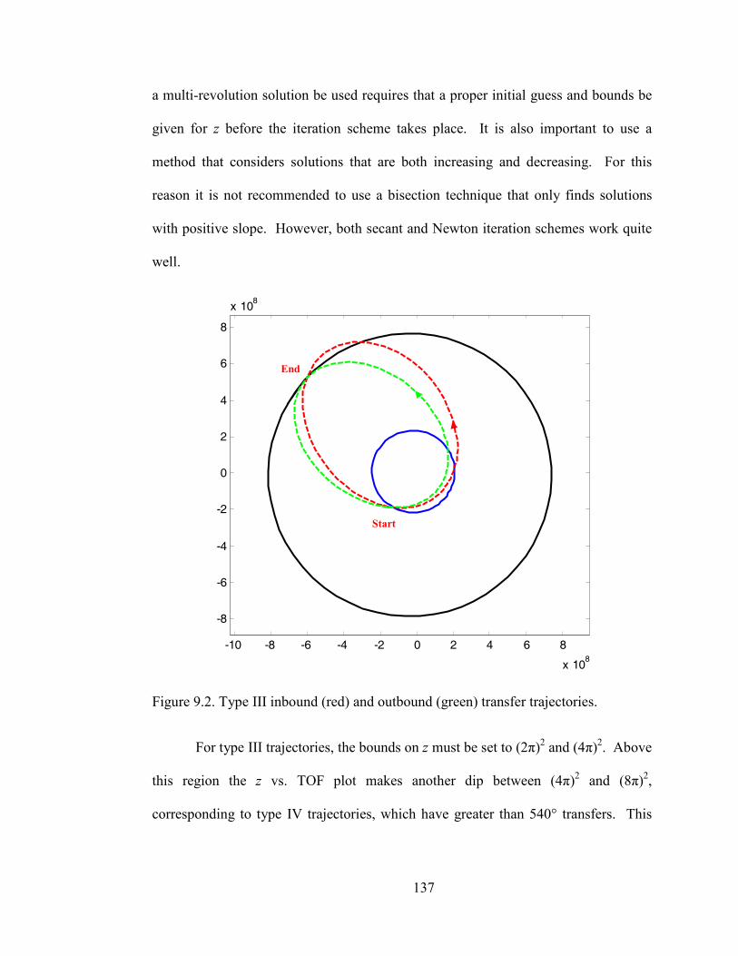
137
a multi-revolution solution be used requires that a proper initial guess and bounds be
given for z before the iteration scheme takes place. It is also important to use a
method that considers solutions that are both increasing and decreasing. For this
reason it is not recommended to use a bisection technique that only finds solutions
with positive slope. However, both secant and Newton iteration schemes work quite
well.
-10 -8 -6 -4 -2 0 2 4 6 8
x 108
-8
-6
-4
-2
0
2
4
6
8
x 108
Figure 9.2. Type III inbound (red) and outbound (green) transfer trajectories.
For type III trajectories, the bounds on z must be set to (2π)2 and (4π)2. Above
this region the z vs. TOF plot makes another dip between (4π)2 and (8π)2,
corresponding to type IV trajectories, which have greater than 540° transfers. This
Start
End

138
trend continues with asymptotes at (16π)2, (32π)2, and so on, marking the boundaries
for higher revolution transfers.
139
10 Appendix D: Tables of V∞ Leveraging Sequences
These tables contain some of the most efficient sequences found during the
Monte Carlo simulations. In each table the total time (in TU35), total ∆V (in VU36),
and resonance sequence are listed. The resonances are listed in decimal form. For
example, “2” is 2:1, “3.75” is 15:4, etc. The sequences begin at V∞ = 0 and progress
outward until a 6:1 resonance with α = 0 is achieved. The zeros after the “6” are
merely place holders in the output.
The sequences where a zero is listed before 6:1 is reached indicates that a
phasing orbit was required. The resonance immediately preceding that zero is a
phasing resonance where no leveraging maneuver is performed. Sequences with
values less than one indicate that a non-tangential maneuver was used. This is where
α does not return to zero after a flyby, and a leveraging maneuver is performed on the
subsequent resonance. The value that is less than one is the magnitude of α in
degrees, divided by 100, for the resonance immediately following.
35 The time units here are the period of the gravity-assist body (P), not P/2π as used in the 3BP.
36 One velocity unit is equal to the circular velocity of the gravity-assist body.
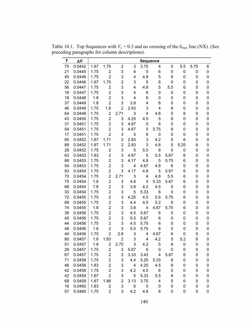
140
Table 10.1. Top Sequences with Vc = 0.3 and no crossing of the δmax line (NX). (See preceding paragraphs for column descriptions).
T ∆∆∆∆V Sequence
75 0.0442 1.67 1.75 2 3 3.75 4 5 5.5 5.75 6
21 0.0445 1.75 2 3 4 5 6 0 0 0 0
45 0.0446 1.75 2 3 4 4.8 5 6 0 0 0
22 0.0446 1.67 1.75 2 3 5 6 0 0 0 0
56 0.0447 1.75 2 3 4 4.8 5 5.5 6 0 0
16 0.0447 1.75 2 3 4 6 0 0 0 0 0
18 0.0448 1.8 2 3 4 6 0 0 0 0 0
37 0.0449 1.8 2 3 3.8 4 6 0 0 0 0
46 0.0449 1.75 1.8 2 2.63 3 4 6 0 0 0
64 0.0449 1.75 2 2.71 3 4 4.8 5 6 0 0
43 0.0450 1.75 2 3 4.25 4.5 5 6 0 0 0
31 0.0451 1.75 2 3 4.67 5 6 0 0 0 0
54 0.0451 1.75 2 3 4.67 5 5.75 6 0 0 0
17 0.0451 1.75 2 3 5 6 0 0 0 0 0
65 0.0452 1.67 1.71 2 2.83 3 4.2 5 6 0 0
89 0.0452 1.67 1.71 2 2.83 3 4.8 5 5.25 6 0
28 0.0452 1.75 2 3 5 5.5 6 0 0 0 0
63 0.0453 1.83 2 3 4.67 5 5.5 5.67 6 0 0
89 0.0453 1.75 2 3 4.17 4.8 5 5.75 6 0 0
54 0.0453 1.75 2 3 4 4.67 4.8 6 0 0 0
83 0.0454 1.75 2 3 4.17 4.8 5 5.67 6 0 0
70 0.0454 1.75 2 2.71 3 4 4.8 5.5 6 0 0
75 0.0454 1.8 2 3 4.6 5 5.33 5.67 6 0 0
68 0.0454 1.8 2 3 3.8 4.2 4.5 5 6 0 0
33 0.0454 1.75 2 3 5 5.33 6 0 0 0 0
72 0.0455 1.75 2 3 4.25 4.5 5.5 5.75 6 0 0
69 0.0455 1.75 2 3 4.4 4.5 5.2 6 0 0 0
74 0.0455 1.8 2 3 3.8 4 4.67 5.75 6 0 0
38 0.0456 1.75 2 3 4.5 5.67 6 0 0 0 0
40 0.0456 1.75 2 3 5.5 5.67 6 0 0 0 0
44 0.0456 1.75 2 3 4.5 5.75 6 0 0 0 0
48 0.0456 1.8 2 3 5.5 5.75 6 0 0 0 0
44 0.0456 1.75 2 2.8 3 4 4.67 6 0 0 0
80 0.0457 1.6 1.83 2 3 4 4.2 5 5.2 6 0
51 0.0457 1.8 2 2.75 3 4.2 5 6 0 0 0
29 0.0457 1.75 2 3 5.67 6 0 0 0 0 0
67 0.0457 1.75 2 3 3.33 3.43 4 5.67 6 0 0
71 0.0458 1.75 2 3 4.4 5.25 5.33 6 0 0 0
46 0.0458 1.83 2 3 4 4.25 4.5 6 0 0 0
42 0.0458 1.75 2 3 4.2 4.5 6 0 0 0 0
42 0.0459 1.67 2 3 5 5.33 5.5 6 0 0 0
69 0.0459 1.67 1.86 2 3.13 3.75 4 5 6 0 0
16 0.0460 1.83 2 3 6 0 0 0 0 0 0
57 0.0460 1.75 2 3 4.2 4.8 6 0 0 0 0
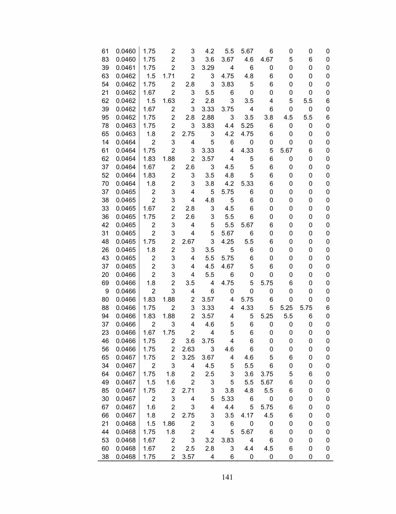
141
61 0.0460 1.75 2 3 4.2 5.5 5.67 6 0 0 0
83 0.0460 1.75 2 3 3.6 3.67 4.6 4.67 5 6 0
39 0.0461 1.75 2 3 3.29 4 6 0 0 0 0
63 0.0462 1.5 1.71 2 3 4.75 4.8 6 0 0 0
54 0.0462 1.75 2 2.8 3 3.83 5 6 0 0 0
21 0.0462 1.67 2 3 5.5 6 0 0 0 0 0
62 0.0462 1.5 1.63 2 2.8 3 3.5 4 5 5.5 6
39 0.0462 1.67 2 3 3.33 3.75 4 6 0 0 0
95 0.0462 1.75 2 2.8 2.88 3 3.5 3.8 4.5 5.5 6
78 0.0463 1.75 2 3 3.83 4.4 5.25 6 0 0 0
65 0.0463 1.8 2 2.75 3 4.2 4.75 6 0 0 0
14 0.0464 2 3 4 5 6 0 0 0 0 0
61 0.0464 1.75 2 3 3.33 4 4.33 5 5.67 6 0
62 0.0464 1.83 1.88 2 3.57 4 5 6 0 0 0
37 0.0464 1.67 2 2.6 3 4.5 5 6 0 0 0
52 0.0464 1.83 2 3 3.5 4.8 5 6 0 0 0
70 0.0464 1.8 2 3 3.8 4.2 5.33 6 0 0 0
37 0.0465 2 3 4 5 5.75 6 0 0 0 0
38 0.0465 2 3 4 4.8 5 6 0 0 0 0
33 0.0465 1.67 2 2.8 3 4.5 6 0 0 0 0
36 0.0465 1.75 2 2.6 3 5.5 6 0 0 0 0
42 0.0465 2 3 4 5 5.5 5.67 6 0 0 0
31 0.0465 2 3 4 5 5.67 6 0 0 0 0
48 0.0465 1.75 2 2.67 3 4.25 5.5 6 0 0 0
26 0.0465 1.8 2 3 3.5 5 6 0 0 0 0
43 0.0465 2 3 4 5.5 5.75 6 0 0 0 0
37 0.0465 2 3 4 4.5 4.67 5 6 0 0 0
20 0.0466 2 3 4 5.5 6 0 0 0 0 0
69 0.0466 1.8 2 3.5 4 4.75 5 5.75 6 0 0
9 0.0466 2 3 4 6 0 0 0 0 0 0
80 0.0466 1.83 1.88 2 3.57 4 5.75 6 0 0 0
88 0.0466 1.75 2 3 3.33 4 4.33 5 5.25 5.75 6
94 0.0466 1.83 1.88 2 3.57 4 5 5.25 5.5 6 0
37 0.0466 2 3 4 4.6 5 6 0 0 0 0
23 0.0466 1.67 1.75 2 4 5 6 0 0 0 0
46 0.0466 1.75 2 3.6 3.75 4 6 0 0 0 0
56 0.0466 1.75 2 2.63 3 4.6 6 0 0 0 0
65 0.0467 1.75 2 3.25 3.67 4 4.6 5 6 0 0
34 0.0467 2 3 4 4.5 5 5.5 6 0 0 0
64 0.0467 1.75 1.8 2 2.5 3 3.6 3.75 5 6 0
49 0.0467 1.5 1.6 2 3 5 5.5 5.67 6 0 0
85 0.0467 1.75 2 2.71 3 3.8 4.8 5.5 6 0 0
30 0.0467 2 3 4 5 5.33 6 0 0 0 0
67 0.0467 1.6 2 3 4 4.4 5 5.75 6 0 0
66 0.0467 1.8 2 2.75 3 3.5 4.17 4.5 6 0 0
21 0.0468 1.5 1.86 2 3 6 0 0 0 0 0
44 0.0468 1.75 1.8 2 4 5 5.67 6 0 0 0
53 0.0468 1.67 2 3 3.2 3.83 4 6 0 0 0
60 0.0468 1.67 2 2.5 2.8 3 4.4 4.5 6 0 0
38 0.0468 1.75 2 3.57 4 6 0 0 0 0 0
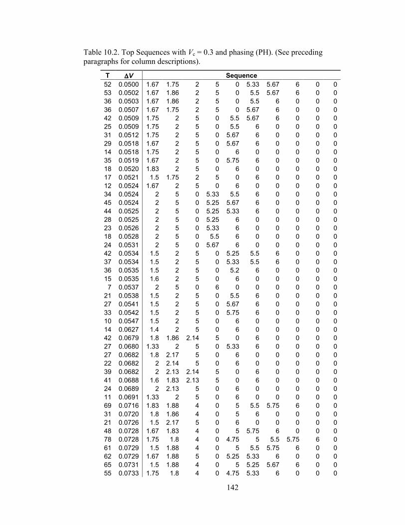
142
Table 10.2. Top Sequences with Vc = 0.3 and phasing (PH). (See preceding paragraphs for column descriptions).
T ∆∆∆∆V Sequence
52 0.0500 1.67 1.75 2 5 0 5.33 5.67 6 0 0
53 0.0502 1.67 1.86 2 5 0 5.5 5.67 6 0 0
36 0.0503 1.67 1.86 2 5 0 5.5 6 0 0 0
36 0.0507 1.67 1.75 2 5 0 5.67 6 0 0 0
42 0.0509 1.75 2 5 0 5.5 5.67 6 0 0 0
25 0.0509 1.75 2 5 0 5.5 6 0 0 0 0
31 0.0512 1.75 2 5 0 5.67 6 0 0 0 0
29 0.0518 1.67 2 5 0 5.67 6 0 0 0 0
14 0.0518 1.75 2 5 0 6 0 0 0 0 0
35 0.0519 1.67 2 5 0 5.75 6 0 0 0 0
18 0.0520 1.83 2 5 0 6 0 0 0 0 0
17 0.0521 1.5 1.75 2 5 0 6 0 0 0 0
12 0.0524 1.67 2 5 0 6 0 0 0 0 0
34 0.0524 2 5 0 5.33 5.5 6 0 0 0 0
45 0.0524 2 5 0 5.25 5.67 6 0 0 0 0
44 0.0525 2 5 0 5.25 5.33 6 0 0 0 0
28 0.0525 2 5 0 5.25 6 0 0 0 0 0
23 0.0526 2 5 0 5.33 6 0 0 0 0 0
18 0.0528 2 5 0 5.5 6 0 0 0 0 0
24 0.0531 2 5 0 5.67 6 0 0 0 0 0
42 0.0534 1.5 2 5 0 5.25 5.5 6 0 0 0
37 0.0534 1.5 2 5 0 5.33 5.5 6 0 0 0
36 0.0535 1.5 2 5 0 5.2 6 0 0 0 0
15 0.0535 1.6 2 5 0 6 0 0 0 0 0
7 0.0537 2 5 0 6 0 0 0 0 0 0
21 0.0538 1.5 2 5 0 5.5 6 0 0 0 0
27 0.0541 1.5 2 5 0 5.67 6 0 0 0 0
33 0.0542 1.5 2 5 0 5.75 6 0 0 0 0
10 0.0547 1.5 2 5 0 6 0 0 0 0 0
14 0.0627 1.4 2 5 0 6 0 0 0 0 0
42 0.0679 1.8 1.86 2.14 5 0 6 0 0 0 0
27 0.0680 1.33 2 5 0 5.33 6 0 0 0 0
27 0.0682 1.8 2.17 5 0 6 0 0 0 0 0
22 0.0682 2 2.14 5 0 6 0 0 0 0 0
39 0.0682 2 2.13 2.14 5 0 6 0 0 0 0
41 0.0688 1.6 1.83 2.13 5 0 6 0 0 0 0
24 0.0689 2 2.13 5 0 6 0 0 0 0 0
11 0.0691 1.33 2 5 0 6 0 0 0 0 0
69 0.0716 1.83 1.88 4 0 5 5.5 5.75 6 0 0
31 0.0720 1.8 1.86 4 0 5 6 0 0 0 0
21 0.0726 1.5 2.17 5 0 6 0 0 0 0 0
48 0.0728 1.67 1.83 4 0 5 5.75 6 0 0 0
78 0.0728 1.75 1.8 4 0 4.75 5 5.5 5.75 6 0
61 0.0729 1.5 1.88 4 0 5 5.5 5.75 6 0 0
62 0.0729 1.67 1.88 5 0 5.25 5.33 6 0 0 0
65 0.0731 1.5 1.88 4 0 5 5.25 5.67 6 0 0
55 0.0733 1.75 1.8 4 0 4.75 5.33 6 0 0 0
143
28 0.0733 1.6 1.83 4 0 5 6 0 0 0 0
25 0.0734 1.5 1.86 4 0 5 6 0 0 0 0
46 0.0734 1.67 1.75 4 0 4.5 5 5.33 6 0 0
68 0.0734 1.5 1.6 1.88 5 0 5.25 5.33 6 0 0
36 0.0735 1.5 1.86 4 0 5 5.5 6 0 0 0
39 0.0735 1.75 1.8 4 0 4.75 6 0 0 0 0
27 0.0736 1.8 4 0 4.67 6 0 0 0 0 0
47 0.0737 1.83 1.88 5 0 5.33 6 0 0 0 0
42 0.0737 1.75 4 0 4.5 5 5.67 6 0 0 0
23 0.0740 1.67 1.8 4 0 5 6 0 0 0 0
34 0.0742 1.67 1.8 4 0 5 5.5 6 0 0 0
60 0.0742 1.8 4 0 4.8 5.75 6 0 0 0 0
62 0.0743 1.67 1.8 4 0 5 5.33 5.75 6 0 0
29 0.0743 1.5 1.6 1.8 4 0 5 6 0 0 0
36 0.0743 1.75 1.8 4 0 5 5.5 6 0 0 0
61 0.0749 1.8 1.86 5 0 5.5 5.75 6 0 0 0
56 0.0751 1.8 4 0 5 5.25 5.67 6 0 0 0
35 0.0754 1.75 4 0 4.75 5 6 0 0 0 0
51 0.0754 1.6 1.83 5 0 5.33 5.5 6 0 0 0
46 0.0755 1.75 4 0 4.75 5 5.5 6 0 0 0
37 0.0755 1.5 1.86 5 0 5.33 6 0 0 0 0
35 0.0756 1.67 1.75 4 0 4.75 6 0 0 0 0
34 0.0757 1.5 1.88 5 0 5.5 6 0 0 0 0
51 0.0757 1.75 4 0 4.75 5 5.33 6 0 0 0
23 0.0757 1.5 1.63 3 0 4 6 0 0 0 0
81 0.0759 1.5 1.63 3 0 4 4.67 5 5.33 5.75 6
30 0.0761 1.75 4 0 4.75 6 0 0 0 0 0
49 0.0762 1.5 1.86 5 0 5.5 5.67 6 0 0 0
32 0.0762 1.5 1.86 5 0 5.5 6 0 0 0 0
21 0.0764 1.67 1.75 4 0 5 6 0 0 0 0
44 0.0765 1.67 1.75 4 0 5 5.75 6 0 0 0
91 0.0766 1.67 1.75 4 0 5 5.2 5.33 5.5 5.67 6
40 0.0767 1.5 3 0 3.57 4 5 6 0 0 0
58 0.0767 1.67 1.75 4 0 5 5.2 5.5 6 0 0
27 0.0769 1.67 4 0 4.33 5 6 0 0 0 0
60 0.0769 1.67 4 0 4.33 4.4 5 5.5 6 0 0
61 0.0769 1.67 4 0 4.33 5 5.5 5.75 6 0 0
68 0.0769 1.5 3 0 3.57 4 5.33 5.67 6 0 0
44 0.0770 1.67 4 0 4.33 5 5.67 6 0 0 0
80 0.0770 1.67 4 0 4.33 4.5 4.6 5 5.25 6 0
38 0.0771 1.5 1.86 5 0 5.67 6 0 0 0 0
36 0.0771 1.5 1.63 3 0 4 4.33 6 0 0 0
56 0.0771 1.5 3 0 3.57 4 5.25 6 0 0 0
27 0.0772 1.8 1.86 5 0 6 0 0 0 0 0
73 0.0773 1.67 4 0 4.33 4.67 5.25 5.33 6 0 0
54 0.0773 1.67 4 0 4.33 5.25 5.5 6 0 0 0
29 0.0773 1.5 1.6 3 0 4 5.5 6 0 0 0
45 0.0773 1.5 1.6 3 0 4 5.33 5.5 6 0 0
44 0.0774 1.5 1.86 5 0 5.75 6 0 0 0 0 47 0.0775 1.6 1.83 5 0 5.75 6 0 0 0 0
144
Table 10.3. Top Sequences with Vc = 0.3 and non-tangential (NT) leveraging. (See preceding paragraphs for column descriptions).
T ∆∆∆∆V Sequence
43 0.0505 1.8 2 0.06 5.25 5.5 6 0 0
30 0.0506 1.75 2 0.06 5.25 6 0 0 0
51 0.0507 1.75 2 0.05 5.2 5.33 6 0 0
62 0.0507 1.83 2 0.05 5.2 5.75 6 0 0
31 0.0507 1.67 1.75 2 0.06 5.67 6 0 0
36 0.0509 1.75 2 0.07 5.4 6 0 0 0
41 0.0509 1.6 1.67 2 0.05 5.2 6 0 0
37 0.0512 1.75 2 0.05 5.6 6 0 0 0
33 0.0512 1.67 2 0.05 5.2 6 0 0 0
26 0.0512 1.75 2 0.06 5.67 6 0 0 0
39 0.0512 1.8 2 0.05 5.6 6 0 0 0
34 0.0515 1.67 2 0.07 5.4 6 0 0 0
7 0.0522 2 0.1 5 6 0 0 0 0
62 0.0523 2 0.05 5.2 5.5 5.75 6 0 0
39 0.0523 2 0.05 5.2 5.5 6 0 0 0
34 0.0524 2 0.06 5.25 5.5 6 0 0 0
51 0.0524 2 0.05 5.2 5.75 6 0 0 0
46 0.0524 2 0.06 5.25 5.75 6 0 0 0
40 0.0525 2 0.06 5.25 5.67 6 0 0 0
28 0.0525 2 0.05 5.2 6 0 0 0 0
23 0.0525 2 0.06 5.25 6 0 0 0 0
44 0.0525 2 0.05 5.2 5.33 6 0 0 0
52 0.0527 2 0.07 5.4 5.75 6 0 0 0
29 0.0528 2 0.07 5.4 6 0 0 0 0
30 0.0531 2 0.05 5.6 6 0 0 0 0
19 0.0531 2 0.06 5.67 6 0 0 0 0
55 0.0537 1.5 2 0.07 5.4 5.75 6 0 0
49 0.0538 1.5 2 0.07 5.4 5.67 6 0 0
32 0.0538 1.5 2 0.07 5.4 6 0 0 0
39 0.0550 2 0.1 5 5.25 5.5 6 0 0
51 0.0551 2 0.1 5 5.25 5.75 6 0 0
28 0.0552 2 0.1 5 5.25 6 0 0 0
39 0.0553 1.4 1.5 2 0.07 5.4 6 0 0
34 0.0598 1.33 1.57 2 0.06 5.67 6 0 0
44 0.0679 1.33 2 0.06 5.25 5.67 6 0 0
34 0.0685 1.33 2 0.05 5.6 6 0 0 0
30 0.0715 1.75 1.8 0.08 4.5 5 6 0 0
42 0.0721 1.75 1.8 0.08 4.5 5.67 6 0 0
95 0.0722 1.8 1.86 0.1 4.8 5.25 5.5 5.67 6
67 0.0722 1.75 1.86 0.1 4.8 5.75 6 0 0
67 0.0724 1.8 1.86 0.1 4.8 5.25 6 0 0
85 0.0724 1.67 1.75 1.83 0.1 4.8 5.25 5.67 6
63 0.0724 1.8 1.86 0.1 4.8 5.67 6 0 0
69 0.0725 1.8 1.86 0.1 4.8 5.75 6 0 0
145
46 0.0726 1.8 1.86 0.1 4.8 6 0 0 0
81 0.0731 1.67 1.75 0.08 4.4 4.75 5 5.75 6
45 0.0731 1.6 1.86 0.1 4.8 6 0 0 0
39 0.0732 1.67 1.75 0.08 4.4 5 6 0 0
28 0.0732 1.8 0.07 4.67 5 6 0 0 0
73 0.0732 1.67 1.75 0.08 4.4 5 5.5 5.75 6
27 0.0733 1.8 1.86 0.1 5 6 0 0 0
92 0.0735 1.67 1.75 0.08 4.4 4.8 5.5 5.75 6
89 0.0736 1.67 1.75 0.08 4.4 5.25 5.5 5.75 6
71 0.0736 1.6 1.83 0.1 4.8 5.5 5.67 6 0
65 0.0736 1.67 1.75 0.08 4.4 5 5.2 6 0
44 0.0736 1.67 1.86 0.05 5.2 6 0 0 0
68 0.0737 1.67 1.75 0.08 4.4 4.6 5.5 6 0
57 0.0738 1.5 1.86 0.1 4.8 5.67 6 0 0
50 0.0738 1.67 1.75 0.08 4.4 5.33 6 0 0
43 0.0739 1.6 1.83 0.1 4.8 6 0 0 0
51 0.0739 1.67 1.75 0.08 4.4 5.67 6 0 0
40 0.0739 1.5 1.86 0.1 4.8 6 0 0 0
57 0.0739 1.67 1.75 0.08 4.4 5.75 6 0 0
34 0.0741 1.67 1.75 0.08 4.4 6 0 0 0
35 0.0741 1.83 0.1 4.8 6 0 0 0 0
21 0.0741 1.75 0.08 4.5 5 6 0 0 0
44 0.0742 1.67 1.75 0.08 4.5 5.75 6 0 0
40 0.0742 1.67 1.75 0.06 4.6 5 6 0 0
63 0.0743 1.67 1.75 0.06 4.6 5 5.75 6 0
70 0.0743 1.75 0.08 4.5 5 5.25 5.5 5.67 6
51 0.0745 1.75 1.8 0.1 4.8 5.5 6 0 0
42 0.0745 1.75 0.08 4.5 5 5.25 6 0 0
49 0.0746 1.75 0.08 4.5 5.33 5.67 6 0 0
56 0.0746 1.75 1.8 0.1 4.8 5.33 6 0 0
32 0.0747 1.75 0.08 4.5 5.33 6 0 0 0
63 0.0747 1.75 1.8 0.1 4.8 5.75 6 0 0
42 0.0748 1.5 1.63 1.75 0.07 4.67 5 6 0
16 0.0749 1.75 0.08 4.5 6 0 0 0 0
49 0.0752 1.8 0.1 4.8 5.33 6 0 0 0
33 0.0753 1.8 0.1 4.8 6 0 0 0 0
40 0.0755 1.6 1.83 0.06 5.25 6 0 0 0
43 0.0755 1.83 1.88 0.06 5.67 6 0 0 0
61 0.0761 1.5 1.71 0.08 4.4 4.8 6 0 0
58 0.0762 1.5 1.83 0.06 5.25 5.75 6 0 0
51 0.0762 1.67 1.75 1.83 0.08 5.6 6 0 0
65 0.0764 1.5 1.63 0.13 3.8 4.17 5 6 0
49 0.0765 1.6 1.86 0.08 5.6 6 0 0 0
70 0.0767 1.67 1.75 0.1 4.8 5.5 5.75 6 0
69 0.0768 1.5 1.63 0.13 3.8 4.17 4.5 6 0
30 0.0771 1.6 1.83 0.08 5.5 6 0 0 0
79 0.0772 1.5 1.67 0.08 4.25 5 5.2 5.75 6
60 0.0773 1.75 1.8 0.07 5.4 5.67 6 0 0
43 0.0773 1.75 1.8 0.07 5.4 6 0 0 0
65 0.0773 1.5 0.09 3.5 4 4.25 4.6 5.5 6
146
Table 10.4. Most efficient sequences for Vc = 0.2.
T ∆∆∆∆V Sequence
37 0.05262 1.5 1.6 1.67 2 3 0.09 5.33 6 0 0 0
58 0.05264 1.4 1.5 1.78 2 0.15 3 0.08 4.4 5 6 0
74 0.05275 1.5 1.8 2 3 4.33 5 5.5 5.6 6 0 0
100 0.05413 1.5 1.6 2 2.71 2.75 3 5 0 5.2 5.75 6
75 0.05421 1.5 1.6 2 2.67 3 0.1 4.8 5.33 5.5 6 0
26 0.05446 1.67 1.75 2 0.13 3 4 0 5 6 0 0
44 0.05451 1.5 2 3 4 5 5.4 6 0 0 0 0
48 0.05456 1.5 1.6 2 2.67 3 0.1 4.8 6 0 0 0
81 0.05457 1.67 1.75 2 2.86 3 0.08 5.25 5.75 6 0 0
61 0.05460 1.5 2 3 4 5.2 5.75 6 0 0 0 0
22 0.05467 1.5 1.67 2 3 0 4 5 6 0 0 0
17 0.05487 1.5 2 3 4 0 5 6 0 0 0 0
66 0.05490 1.67 1.75 2 0.13 3 5 0 5.25 5.75 6 0
37 0.05491 1.67 2 3 4 5.75 6 0 0 0 0 0
38 0.05493 1.67 1.89 2 3 0.1 5.5 6 0 0 0 0
17 0.05494 1.6 2 3 4 6 0 0 0 0 0 0
61 0.05495 1.5 1.71 2 0.08 3.2 3.5 4 4.25 6 0 0
61 0.05496 1.5 2 3 4.5 5 5.33 5.75 6 0 0 0
43 0.05499 1.67 1.75 2 0.13 3 5 0 5.25 6 0 0
37 0.05500 1.5 2 3 4 4.5 5.33 6 0 0 0 0
12 0.05505 1.5 2 0.14 3 4 6 0 0 0 0 0
26 0.05514 1.67 2 3 3.5 4 5 6 0 0 0 0
54 0.05531 1.5 2 3 0.05 4.75 5.4 6 0 0 0 0
38 0.05532 1.5 2 3 0.07 4.67 5.33 6 0 0 0 0
45 0.05532 1.4 1.43 1.75 2 0.13 3 5 0 5.5 6 0
41 0.05536 1.5 2 3 0.09 5.33 5.67 6 0 0 0 0
48 0.05540 1.5 2 3 0.06 4.6 5.67 6 0 0 0 0
34 0.05543 1.5 2 3 5 0 5.25 6 0 0 0 0
41 0.05544 1.5 2 3 5 0 5.6 6 0 0 0 0
59 0.05547 1.5 2 0.13 3 0.1 4.8 5.4 6 0 0 0
13 0.05558 1.5 2 3 5 0 6 0 0 0 0 0
55 0.05561 1.5 2 3 4 0 4.75 4.8 6 0 0 0
26 0.05562 1.5 2 3 4 0 4.67 6 0 0 0 0
62 0.05563 1.5 2 2.71 3 4.5 5.2 6 0 0 0 0
18 0.05563 1.6 2 3 0.1 5 6 0 0 0 0 0
83 0.05564 1.5 1.67 2 0.19 3.8 4.5 4.6 5 5.67 6 0
109 0.05566 1.5 2 2.78 3 4.33 5.2 5.25 5.33 6 0 0
51 0.05568 1.75 2 3 3.8 4 5 5.5 6 0 0 0
37 0.05570 1.5 1.6 2 3 0 3.5 4.5 5 6 0 0
43 0.05575 1.75 2 3 4 5.4 6 0 0 0 0 0
70 0.05579 1.67 2 3 5 0 5.4 5.6 6 0 0 0
47 0.05580 1.5 2 2.67 2.86 3 0.1 5.5 6 0 0 0
59 0.05581 1.67 2 3 5 0 5.25 5.75 6 0 0 0
57 0.05583 1.5 2 0.17 3 5 0 5.4 5.67 6 0 0
44 0.05585 1.5 2 3 4.17 5.5 6 0 0 0 0 0
97 0.05585 1.5 2 2.63 3 0.1 4.8 5.25 5.75 6 0 0
78 0.05587 1.5 1.56 1.86 2 2.78 4 5.67 6 0 0 0
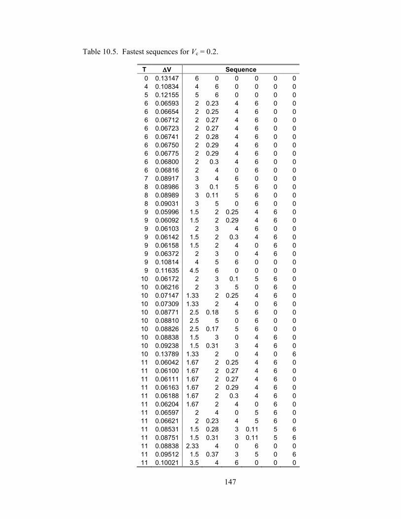
147
Table 10.5. Fastest sequences for Vc = 0.2.
T ∆∆∆∆V Sequence
0 0.13147 6 0 0 0 0 0
4 0.10834 4 6 0 0 0 0
5 0.12155 5 6 0 0 0 0
6 0.06593 2 0.23 4 6 0 0
6 0.06654 2 0.25 4 6 0 0
6 0.06712 2 0.27 4 6 0 0
6 0.06723 2 0.27 4 6 0 0
6 0.06741 2 0.28 4 6 0 0
6 0.06750 2 0.29 4 6 0 0
6 0.06775 2 0.29 4 6 0 0
6 0.06800 2 0.3 4 6 0 0
6 0.06816 2 4 0 6 0 0
7 0.08917 3 4 6 0 0 0
8 0.08986 3 0.1 5 6 0 0
8 0.08989 3 0.11 5 6 0 0
8 0.09031 3 5 0 6 0 0
9 0.05996 1.5 2 0.25 4 6 0
9 0.06092 1.5 2 0.29 4 6 0
9 0.06103 2 3 4 6 0 0
9 0.06142 1.5 2 0.3 4 6 0
9 0.06158 1.5 2 4 0 6 0
9 0.06372 2 3 0 4 6 0
9 0.10814 4 5 6 0 0 0
9 0.11635 4.5 6 0 0 0 0
10 0.06172 2 3 0.1 5 6 0
10 0.06216 2 3 5 0 6 0
10 0.07147 1.33 2 0.25 4 6 0
10 0.07309 1.33 2 4 0 6 0
10 0.08771 2.5 0.18 5 6 0 0
10 0.08810 2.5 5 0 6 0 0
10 0.08826 2.5 0.17 5 6 0 0
10 0.08838 1.5 3 0 4 6 0
10 0.09238 1.5 0.31 3 4 6 0
10 0.13789 1.33 2 0 4 0 6
11 0.06042 1.67 2 0.25 4 6 0
11 0.06100 1.67 2 0.27 4 6 0
11 0.06111 1.67 2 0.27 4 6 0
11 0.06163 1.67 2 0.29 4 6 0
11 0.06188 1.67 2 0.3 4 6 0
11 0.06204 1.67 2 4 0 6 0
11 0.06597 2 4 0 5 6 0
11 0.06621 2 0.23 4 5 6 0
11 0.08531 1.5 0.28 3 0.11 5 6
11 0.08751 1.5 0.31 3 0.11 5 6
11 0.08838 2.33 4 0 6 0 0
11 0.09512 1.5 0.37 3 5 0 6
11 0.10021 3.5 4 6 0 0 0
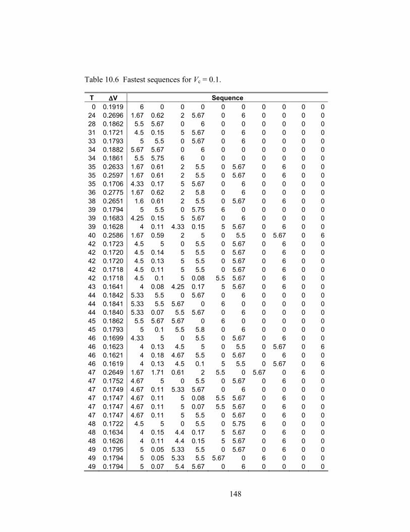
148
Table 10.6 Fastest sequences for Vc = 0.1.
T ∆∆∆∆V Sequence
0 0.1919 6 0 0 0 0 0 0 0 0 0
24 0.2696 1.67 0.62 2 5.67 0 6 0 0 0 0
28 0.1862 5.5 5.67 0 6 0 0 0 0 0 0
31 0.1721 4.5 0.15 5 5.67 0 6 0 0 0 0
33 0.1793 5 5.5 0 5.67 0 6 0 0 0 0
34 0.1882 5.67 5.67 0 6 0 0 0 0 0 0
34 0.1861 5.5 5.75 6 0 0 0 0 0 0 0
35 0.2633 1.67 0.61 2 5.5 0 5.67 0 6 0 0
35 0.2597 1.67 0.61 2 5.5 0 5.67 0 6 0 0
35 0.1706 4.33 0.17 5 5.67 0 6 0 0 0 0
36 0.2775 1.67 0.62 2 5.8 0 6 0 0 0 0
38 0.2651 1.6 0.61 2 5.5 0 5.67 0 6 0 0
39 0.1794 5 5.5 0 5.75 6 0 0 0 0 0
39 0.1683 4.25 0.15 5 5.67 0 6 0 0 0 0
39 0.1628 4 0.11 4.33 0.15 5 5.67 0 6 0 0
40 0.2586 1.67 0.59 2 5 0 5.5 0 5.67 0 6
42 0.1723 4.5 5 0 5.5 0 5.67 0 6 0 0
42 0.1720 4.5 0.14 5 5.5 0 5.67 0 6 0 0
42 0.1720 4.5 0.13 5 5.5 0 5.67 0 6 0 0
42 0.1718 4.5 0.11 5 5.5 0 5.67 0 6 0 0
42 0.1718 4.5 0.1 5 0.08 5.5 5.67 0 6 0 0
43 0.1641 4 0.08 4.25 0.17 5 5.67 0 6 0 0
44 0.1842 5.33 5.5 0 5.67 0 6 0 0 0 0
44 0.1841 5.33 5.5 5.67 0 6 0 0 0 0 0
44 0.1840 5.33 0.07 5.5 5.67 0 6 0 0 0 0
45 0.1862 5.5 5.67 5.67 0 6 0 0 0 0 0
45 0.1793 5 0.1 5.5 5.8 0 6 0 0 0 0
46 0.1699 4.33 5 0 5.5 0 5.67 0 6 0 0
46 0.1623 4 0.13 4.5 5 0 5.5 0 5.67 0 6
46 0.1621 4 0.18 4.67 5.5 0 5.67 0 6 0 0
46 0.1619 4 0.13 4.5 0.1 5 5.5 0 5.67 0 6
47 0.2649 1.67 1.71 0.61 2 5.5 0 5.67 0 6 0
47 0.1752 4.67 5 0 5.5 0 5.67 0 6 0 0
47 0.1749 4.67 0.11 5.33 5.67 0 6 0 0 0 0
47 0.1747 4.67 0.11 5 0.08 5.5 5.67 0 6 0 0
47 0.1747 4.67 0.11 5 0.07 5.5 5.67 0 6 0 0
47 0.1747 4.67 0.11 5 5.5 0 5.67 0 6 0 0
48 0.1722 4.5 5 0 5.5 0 5.75 6 0 0 0
48 0.1634 4 0.15 4.4 0.17 5 5.67 0 6 0 0
48 0.1626 4 0.11 4.4 0.15 5 5.67 0 6 0 0
49 0.1795 5 0.05 5.33 5.5 0 5.67 0 6 0 0
49 0.1794 5 0.05 5.33 5.5 5.67 0 6 0 0 0
49 0.1794 5 0.07 5.4 5.67 0 6 0 0 0 0