En-Route Sector Metering using a Game-theoretic Approach

Goutam Satapathy*, Vikram Manikonda*, John Robinson#, Todd Farley#

*Intelligent Automation Inc. #NASA Ames Research Center7519 Standish Place, Suite 200 Moffett Field, CA 94035-1000

Rockville, Maryland 20879 jerobinson@~rc.nasa.govgoutam@i-a-i.cora, vikram@i-a-i.com ffarle¥@~rc.nasa.gov

AbstractCurrently, Traffic Management Coordinators in theAir Route Traffic Control Centers establish flowconstraints at various sector meter fixes, based ontheir best estimates of the predicted traffic demandinto their sector. Sector flow rates are not coordinatedbetween neighboring sectors or centers. Incorrectsector metering rates can lead often lead to a cascadeeffect resulting in delays in the schedules of aircraftseveral sectors away. In this paper we develop anapproach for dynamic sector metering based on gametheory. The approach is based on a Bayesian gamewith communication, wherein the sectors determinemutually beneficial metering rates (based oncollaboration and exchange of metering rates andnegotiated Scheduled Times of Arrival) chosen so asto optimize delay, controller workload and capacity.We formalize the model for a simplified scenarioconsisting of two sectors belonging to two differentcenters, attempting to set the flow rates at theirboundaries. The simplified models for the two-player(sector) game capture the coupling of dynamicsbetween the two sectors and possible interactionsbetween incoming and outgoing traffic flows. Theinbound aircraft from other sectors and outbound flowrate restriction to other sectors are generated from astochastic time series model. To demonstratefeasibility we implement our approach on a simplifiedversion of agent-based decision support to capturesinter center/sector communication and decentralizeddecision-making

Introduction

As air traffic congestion and delay have increased in thepost-deregulation era, the air transportation community hassought to identify more efficient methods of Traffic FlowManagement (TFM) in order to best utilize existingcapacity. Advanced TFM strategies have the potential toimprove system throughput and reduce delay withoutrequiting substantial rework of the National AirspaceSystem (NAS) infrastructure (e.g., airspace redesign,Communication, Navigation and Surveillance (CNS)upgrades, etc.) and without imposing new aircraft equipagerequirements.

Copyright © 2000, American Association for Artificial Intelligence(www.aaai.org). All rights reserved.

Currently, Traffic Management Coordinators (TMCs) the Air Route Traffic Conlrol Centers (ARTCC) establishflow constraints at various sector meter fixes, based ontheir best estimates of the predicted traffic demand, orsectors affected by adverse weather conditions. Arrivalrates into a sector are usually determined for sectors closeto airports with high demand, and these rates typically flowdown (radially outward) to en route sectors. Typicallycontrollers add a safety buffer to this rate to accommodatefor any unforeseen circumstances. Sector flow rates are notcoordinated between neighboring sectors or centers basedon the estimated demand on their sectors. Furthermore,metering times at sectors are assigned based on miles-in-trail restrictions (distance-based spacing). While thisapproach works reasonably well for low traffic densities,for higher densities (coupled with the dynamics anduncertainty of the traffic) this approach fails. Inappropriatesector metering rates near a busy airport can often lead to acascade effect resulting in delays in the schedules ofvarious aircraft several sectors away. In addition, it hasbeen observed that fixed miles-in-trail restrictions based onquantization to maintain the metering rates can beinefficient. Controller workload can be improved by givingthe controller the flexibility to impose variable in-trailrestrictions between aircraft, as long as an average meteringrate over a certain duration is maintained, and safety is notcompromised.

Time-based spacing (or "metering") of arrival traffic flowshas been shown to be more efficient than distance-basedspacing, or "in-trail restrictions," as shown by Sokkappa ina theoretical study (Sokakapa. 1989). Sokkappa’s findingswere validated by Swenson, who documented significantimprovements in delay and throughput versus in-trailspacing using NASA’s Traffic Management Advisor(TMA) in operational field tests at Dallas-Fort WorthInternational Airport (DFW) (Swenson, Hoang, et. 1997)

Researchers at NASA Ames Research Center are pursuinga distributed scheduling concept to implement time-basedmetering in constrained, transition airspace (Farley, Foster,Hoang and Lee 2001). Instead of relying on a single,monolithic scheduler to compute a workable and efficientschedule for the entire region, as is the ease for currenttime-based metering systems, a distributed scheduling

66

From: AAAI Technical Report WS-02-06. Compilation copyright © 2002, AAAI (www.aaai.org). All rights reserved.

scheme relies on a loosely integrated network ofschedulers, each governing small airspace regions. Ascheduler might govern an area as small as a singleairspace sector or as large as an enroute Center. Theenvisioned time-based metering operation will be moresensitive to local ATC constraints and goals, but will stillenable facilities to implement an efficient, time-basedmetering approach to air traffic management on a regionalscale.

A key challenge in this work is to determine how---and towhat extent--to couple the distributed schedulers in orderto generate a set of schedules which are individuallyworkable and collectively beneficial. That is, collectivelythey produce a significant throughput benefit.

This paper develops a game-theoretic approach forcoupling distributed scheduling algorithms. The approachis based on a Bayesian game with communication, whereindistributed schedulers negotiate acceptance rates tooptimize system-wide delay, controller workload, andthroughput. One instance of the scheduler is assumed to becomputing trajectory projections (estimated boundary-crossing times, or ETAs (Estimated Time of Arrival)) each defined airspace region. The ETAs are exchangedbetween neighboring agents and are compared againstnegotiated acceptance rates. Overflow situations areresolved by negotiating changes in acceptance rates or byassigning delay to the offending aircraft. For the purposesof this initial investigation, a model was formalized basedon a simplified airspace consisting of two neighboringsectors (Figure 1). The sectors set acceptance rates forarrivals across the shared boundary to their respectivesector. This simplified model for a two-player (i.e., two-sector) game captured the coupling of dynamics betweenthe two sectors, and it captured the possible interactions

} ulanIImmmm~mulllllmu¯~I

oj

J

Figure 1: A layout of the airwa~,s in two sectors for the twoplayer game-theoretic model for sector metering

between incoming and outgoing traffic flows. The inboundaircraft from other (non-playing) sectors and the outboundflow rate restrictions imposed by those other sectors weregenerated from a stochastic time-series model. Themetering times assigned within each sector to comply withthe negotiated acceptance rates were not based upon fixed,in-trail spacing restrictions. Rather, they were based uponassignment of minimum delay subject to the negotiated

acceptance rates and minimum separation requirementsonly. Uncertainty in arrival time estimates was included.Low fidelity models for computation of estimated andscheduled boundary-crossing times (ETAs and STAs,(Scheduled Time of Arrival) respectively), trajectoryconflicts, and controller advisories were also developed. Asimplified implementation of the algorithms is adopted forthis study, capturing inter-sector communication anddecentralized decision-making.

Due to space restriction, we only briefly describe thedomain. Readers may refer to (Nolan, 1994) for a moredetailed description of current NAS operations.

Notation

SiC" : Sector i in center Cu

mf : Sector meter fix (inbound or outbound)ctrl: A control point (A control point is an intersection

or merging point of two airways or a bifurcationpoint of an airway).

m,: The indices of the inbound meter fixes withrespect to the sector

mo: The indices of the outbound meter fixes withrespect to the sector

r=y, r,,,, rmo : The sector meter fix flow rate through

meter fix mfor meter fix indexed by m~ or moAt: The time unit in the specified flow rate (i.e., 10

minutes if the flow rate is specified as 4/10minutes).

sarc,: Sector arrival rate - the rate at which aircraft

enter the sector S/c" . This is equal to the sum of

flow rates into the sector S/c’- E r,,, .

sdrc~ : Sector departure rate - the rate at which

aircra~ depart the sectorsc" . This is equal to the

sum of flow rates from the sector S/C" into other

sectors- E r,,o-mo E~u

c : The capacity of a sector - the maximum numberof aircraft that can be present in a sector at agiven time. It differs from sector to sectordepending the sector controller’s ability tomanage aircraftThe absolute value of time when a stage gamestarts. (The game theoretic approaches proposedfor the sector metering problem consists ofseveral stage games and is played an infinitenumber of times.)The duration of the stage game

to~

AT:

67

s: The minimum aircraft separation distance basedon safety requirements

v,,~: The maximum cruise speed of an aircraft.v~n: The minimum cruise speed of an aircraft.

The minimum separation time that must be keptbased on FAA’s restriction on the minimumseparation distance and the assumption ofuniform cruise speed maintained by all aircraft(Note that 6 is not same s/v,=).

j, k: The aircraft are indexed in such a way that thePSTA of a low indexed aircraft is earlier than thePSTA of a higher indexed aircraft.

!: A control point in sector’s airways. The controlpoints are indexed as/1, 12, .... li, ... such that theSTAs of the incoming aircraft must bedetermined at li before l~+1.

du, :The distance between two control points.

d,,,m, :The distance between two meter fixes.dmd" :The distance between a meter fix and a control

point.aj,m, :Thefh aircraft entering at meth inbound meter fix

ETAo~,mf : Expected Time of Arrival of an aircrafljat a meter fix mf, a control point, inbound oroutbound meter fix

STAoj,~.mf : Scheduled Time of Arrival of an aircraftj

at a meter fix mf(STA is always equal or greaterthan ETA)

PSTAoj,,,,m, : Predicted STA of the aircraft aj,m, at

meth inbound meter fix such that PSTAoj,~,mr <

PSTA%~.,,,m. (Predicted STAs are used only

for optimization)

PSTAo/~,t, : Predicted STA of the aircraft a/,me at lwcontrol point. (Predicted STAs are used only foroptimization)

PSTAoj,.,,m,: Predicted STA of the aircraft a/,m, at

moth outbound meter fix. (Predicted STAs areused only for optimization)

PETA%,,.mo : Predicted ETA of the aircraft a/,me at

moth outbound meter fix, given that

PETAoj~.m, = PSTAoj,,,mt " (Predicted ETAs

are used only for optimization)B(/, u, at, az): A beta probability distribution over l_<x_<

u, where at and a2 are the two shape parameters

Formulation of the sector metering problem asa game-theoretic problem

Game-theoretic models are well suited to determiningsector metering rates across sector boundaries as thisinvolves negotiation between the sectors. It is only bynegotiating the flow rates that sector controllers can reducetheir workload and increase airspace safety. For example,one sector can negotiate with another sector to set a flowrate so that the former sector controller does not getoverloaded with advisories, while the latter sector does notobtain any significant increase in its workload by holdingor delaying aircraft. In this paper we formalize ourapproach using a simplified scenario consisting of twosectors belonging to two different centers, attempting to setthe flow rates at their boundary. The simplified model forthe two-player (sector) game captures the coupling dynamics between the two sectors and possible interactionsbetween incoming and outgoing traffic flows. Figure 1shows the layout of the scenario chosen as a basis of ourformulation.

In Figure 1 S~/" denotes Sector i in center u, rnf denotesthe sector meter fix, ctri denotes a control point. The solidand the dashed lines show airways in the west-east andeast-west directions respectively. The problem in thiscontext is described as

The sectors Scl and SIq play a game to set an

equilibrium flow (acceptance) rate across their sectorboundary, that should be maintained for duration ofAT seconds into the future. After the AT seconds,they play the game again to set the sector flow ratesfor the next AT seconds.

The flow rate is said to be in equilibrium if, given rmL, thesector Sq cannot change rmf’ in order to increase itsutility, and given rmf’ the sector "Sc2 cannot change rmf~ in

order to increase its y utility. Here rm/, denotes the sectormeter fix flow rate through the meter fix. Note that we haveassumed that the two sectors lie in two different centers. Inthis paper, we model the game as a Bayesian game withCommunication.

Bayesian Game with CommunicationIn this formulation, the game consists of two instances ofTMA, one for each sector controller deciding a rate that isfixed for a duration of AT see (the duration of the game).Each controller will "push" aircraft into the other sectorand schedule aircraft to the sector boundary such that theactual time of arrival at the sector boundary conforms tothe rate (action). Note that "conforming to a flow rate" an important part of the action. For example, if the decisionis to push 2 aircraft per AT, then the sector can push thetwo aircraft immediately, one after the other, and not sendany aircraft for the rest of the interval. Alternatively, the

68

sector could send one aircraft at the beginning of theinterval and the other towards the end. The way the sectorconforms to the flow rate will affect the utility of the othersector. Figure 2 summarizes the various components of thegame.

This game can be modeled as a strategic game withincomplete information. Recall, in a strategic game, playerstake actions simultaneously and independently. In a gamewith incomplete information (i.e., payoff/ utility due totheir actions are not known to each other - Bayesiangames) and absence of common knowledge (i.e., priorprobabilities of the opponents’ action that is known to orassumed by each player is not a common knowledge), thenotion of equilibrium is hard to define. In fact, the gameswithout common knowledge played by two players can bedescribed as each player playing distinctly different gameswithout each other’s knowledge and hence equilibriumcannot be defined in such cases. Therefore, we transformthe Bayesian game to be played by the sector

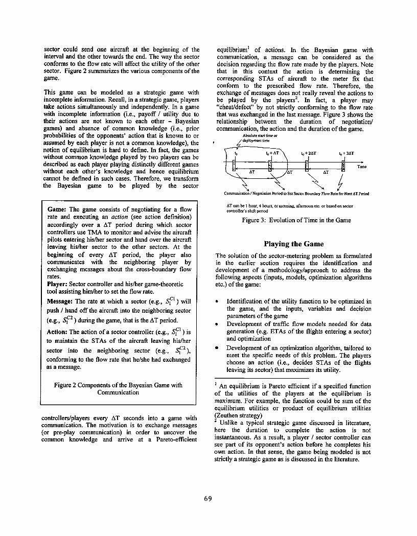
Game: The game consists of negotiating for a flowrate and executing an action (see action definition)accordingly over a AT period during which sectorcontrollers use TMA to monitor and advise the aircraftpilots entering his/her sector and hand over the aircraftleaving his/her sector to the other sectors. At thebeginning of every AT period, the player alsocommunicates with the neighboring player byexchanging messages about the cross-boundary flowrates.Player: Sector controller and his/her game-theoretictool assisting him/her to set the flow rate.

Message: The rate at which a sector (e.g., ci )will

push / hand off the aircraft into the neighboring sector

(e.g., S~t2 ) during the game, that is the AT period.

Action: The action of a sector controller (e.g., cl )is

to maintain the STAs of the aircraft leaving his/her

sector into the neighboring sector (e.g., SC2),conforming to the flow rate that he/she had exchangedas a message.

Figure 2 Components of the Bayesian Game withCommunication

controllers/players every AT seconds into a game withcommunication. The motivation is to exchange messages(or pre-play communication) in order to uncover thecommon knowledge and arrive at a Pareto-efficient

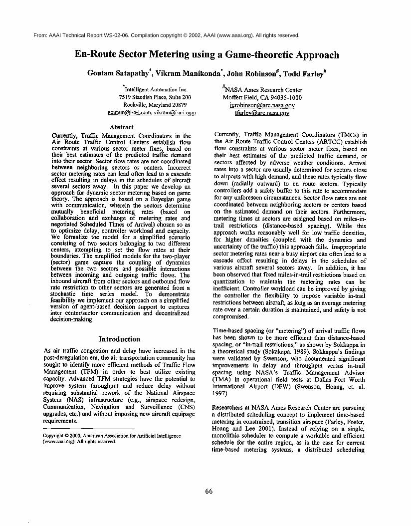
equilibrium ~ of actions. In the Bayesian game withcommunication, a message can be considered as thedecision regarding the flow rate made by the players. Notethat in this context the action is determining thecorresponding STAs of aircraft to the meter fix thatconform to the prescribed flow rate. Therefore, theexchange of messages does not really reveal the actions tobe played by the players z. In fact, a player may"cheat/defect" by not strictly conforming to the flow ratethat was exchanged in the last message. Figure 3 shows therelationship between the duration of negotiation/communication, the action and the duration of the game.

Absolute start time or

7T

~’xAT

Communication / Negotiation Period to Set Sector Botmdary Flow Rate for Next AT Period

AT can be I hour, 4 hours, or morning, aftemoon etc. or based on sector¢or~oller’s shift Ix’riod

Figure 3: Evolution of Time in the Game

Playing the Game

The solution of the sector-metering problem as formulatedin the earlier section requires the identification anddevelopment of a methodology/approach to address thefollowing aspects (inputs, models, optimization algorithmsetc.) of the game:

¯ Identification of the utility function to be optimized inthe game, and the inputs, variables and decisionparameters of the game

¯ Development of traffic flow models needed for datageneration (e.g. ETAs of the flights entering a sector)and optimization

¯ Development of an optimization algorithm, tailored tomeet the specific needs of this problem. The playerschoose an action (i.e., decides STAs of the flightsleaving its sector) that maximizes its utility.

An equilibrium is Pareto efficient if a specified functionof the utilities of the players at the equilibrium ismaximum. For example, the function could be sum of theequilibrium utilities or product of equilibrium utilities

IZeuthen strategy)Unlike a typical strategic game discussed in literature,

here the duration to complete the action is notinstantaneous. As a result, a player / sector controller cansee part of its opponent’s action before he completes hisown action. In that sense, the game being modeled is notstrictly a strategic game as is discussed in the literature.

69

In the following subsections we discuss the technicalapproach adopted in this paper to address these aspects ofthe game

Sector Utility

We measure a sector’s utility as a wei~ted sum of thefollowing elements (e.g., for sector S~ , components ofthe utility function are):1. Aircraft delay due to traffic, i.e.

E E PSTAaia~.mo -PETAaj~",’too ]for each

aircraft ay,m, leaving the sector at a meter fix

indexed by mo

2, Ratio of estimated number of aircraft at agiven time to capacity, i.e.

( [x°+( E r=- E rmo)XAT]/cl" E rra,

(same as Sarsc. ) and E rmo (same as sdrsc. )moEff"

are the arrival and departure rates of the sectorand c is the capacity of the sector. Xo is the numberof aircraft at the beginning of AT period, i.e., justprior to to.

3. Workload on the sector controller (Number ofadvisories issued)

Variables, and Decision parametersThe variables and decision parameters of interest to us inthis game include capacity, sector arrival rate, sectordeparture rate, ETAs and STAs to meter fixes. A keydesign issue is the ability to either measure or accuratelyestimate these variables. In some settings, some of theseparameters can be directly obtained from high fidelityTMA tools such as Center-TRACON Automation System(CTAS) (Erzberger 1994). However, for the purpose of investigation, we developed some simple approaches todetermine these parameters.

l, Capacity (c): This is an upper bound on the number aircraft that can be present in a sector at a given time,and is limited by the ability of the sector controller tomanage more that a certain number of aircraft. Withimproved decision support tools, it is expected that thisnumber will increase.

2. sar: The Sector arrival rate is the rate at which aircraftare entering into a sector, sar is the sum of the sector

inflow rates. Thus, sarff, = rmf° + r,,fc + r,,f, and

sar~2 = rmf" + r~f f + rmfy .In this paper, rmA , rmA , r~f ,and rmff are calculated from a time series model that

predicts the inflow rate through the inbound meter fixfor every AT period. These flow rates are notnegotiable, rmf. and r,,,fyon the other hand are

negotiable and are determined through a stage game.

3. sdr: The sector departure rate is the rate at which theaircraft are departing a sector, sdr is the sum of sectoroutflow rates. Thus, sdrff, = rmA + rmfa + rmfy, and

sdrs~12 =rmfg +rmA +rraf~ In the proposed set up

rmA , rmfa, rmf , and rmfh are calculated for every game

(i.e., for every AT period) based on a time seriesmodel. These rates are also not negotiable. Based onthe set-up of the game, we may consider some rates ascompletely inflexible (hard constraints) and some thatcan change subject to a penalty.

4. PETAoj,~,,,o : The Predicted ETA is the ETA of anaircraft ay.m" (that has not yet entered the sector’s

airspace) at the outbound meter fix mo,. Note thatETAs are calculated as soon as the aircraft enters thesector’s airspace. ETAs of the aircraft at the sector

boundary leaving the sectors Scl and Slc2 are

typically calculated using extensions of the RouteAnalyzer (RA) and Trajectory Synthesis (TS) modulesof the CTAS - Dynamic Planner (DP) (Wong 2000).These tools must be used to calculate PETAs too.However, in our experimental setup, we calculate thePETAs of the aircraft leaving the sectors S1c~ and

Sc2 based on a simple calculation that does not

consider speed restriction at merging points and therestrictions due to aircraft models and weather modelsin the calculation of PETAs, as is done currently withCTAS tools.

5. PSTAojm,mo : The Predicted STA of an aircraft at a

meter fix or control point is the STA of the aircraft thathas not yet entered the sector’s airspace, but ispredicted to enter the sector airspace through aninbound meter fix at a certain time in the future.Hence, PSTA of that aircraft is calculated assuming

the entry-time of several such aircraft. PSTAo/m.m, is

used to denote the PST of an aircraft aj,m, at the

inbound meter fix me. PSTA~j~,,,m, is calculated given

the flow rate rm, (which in turn is given by a time

7O

.

series). Given PSTAaj,~.m, of several such aircraft for

all inbound meter fixes, PSTAaj,~ :,o at the outbound

meter fLX mo can be computed using extensions ofexisting tools such as the DP. While the use of DP willprovide a more accurate computation of PSTAs, due totime constraints in this effort we used relatively lowfidelity heuristics to determine the PSTAs.

We measure the sector controller workload by thenumber of advisories issued by the controller and thecomplexity of those advisories (i.e., must the aircraftbe prescribed a holding pattern or does it need to bediverted before it is returned to the original airway?).We assume that an advisory is issued when anaircraft’s STA at any control point or exit point is notequal to its ETA. The complexity of the advisory ishard to measure, and at this stage of the developmentwe do not consider complexity while computing theworkload. Any advisory that results in a holdingpattern is treated with an equal weight.

Repeated Strategic Bayesian GameA Bayesian game with communication is similar to anextensive game (Osborne and Rubinstein 1994). In thecase of an extensive game, one player exchanges amessage, the other player responds with a message, and thisexchange continues for a finite number of iterations until aterminal state is reached. The players then take the actionsimultaneously. Every AT seconds (duration of the game),the game with communication is played in the extensiveform as follows (since the Bayesian game is played afterevery AT, it is called a repeated Bayesian game):

1. A sector, say SC’ predicts rmL, calculatesoptimal rmf~ and exchanges it with Sc’ . This

involves

a. Predicting PSTA~j,/x.mL of each aircraft

aj,~L using a set of probability distributions

that conforms to rmL.

b. Calculating optimal PSTA~/,.,.mfy using

PSTAo,,.:r.mL

c. Calculating rmfy using PSTA~j,,,.mf~ and

sending r,,f, to Sc2.

2.Given rsf r, Sc2 calculates an optimal rmL and

exchanges it with Sc’ .

3.Now Slq calculates rmf~ using the given r,,fx and

SO on

The game reaches a terminal point when, given the arrivalrate from the other sector, a sector’s calculated rate ofdeparture to the other sector remains the same as thatcomputed earlier. Figure 4 shows a tree called an extensive

Figure 4: Extensive game tree of the Bayesian game withcommunication

tree representing the sequential actions of each sector-player. The design of the game involves desiL, ning theextensive tree in such a way that it leads to fasterconvergence to a terminal point.

In the above description of the Bayesian game withcommunication as an extensive game, the game starts withonly one of the sector players initiating a messageexchange (Satapathy 1999). However, in a strategic gameform of the Bayesian game with communication, theprediction and computation is started by both sectorssimultaneously and independently. Hence, in a strategicgame form of the Bayesian game, two such extensive gametrees can be constructed that progress simultaneously. Theconvergence occurs when both trees lead to a terminalpoint simultaneously. Note that it is possible that we maybe unable to design the game such that it converges. Insuch a case, we impose a hard constraint on the number oftimes the messages can be exchanged and study the Pareto-efficient equilibrium of the strategic game played after theexchange of messages. The design task requiresdetermining suitable constraints on the number of times themessages can be exchanged so that it results in equilibriumcloser to the Pareto-efficient equilibrium. In this paper, weadopt a strategic form of the Bayesian game discussedabove. The primary tasks associated with this game-theoretic formulation of determining equilibrium flow rateis to develop algorithms to:

1. Predict a probability distribution over the differentpossible sets of arrival times of the aircraft arrivingfrom the neighboring sector that conforms to a flowrate.

2. Calculate the optimal outbound flow rate given all theconstraints discussed in formulation.

71

Development of traffic flow models needed fordata generation and optimization

Figure 5 presents the details of input data required foroptimization to compute the flow rate. Details with respectto the sectorslCi, are shown. The inputs are:

1. The inbound flow rates at the meter fixes mfa and

mfc, and PSTAs conforming to these flow rates.

2. The inbound flow rate at the meter fix mfx from the

sector Sc2 and the PSTAs conforming to the flow rate.

3. The outbound flow rate at the meter fixes mfb and

tufa that the sector controller Slq must maintain.

Based on this input data, the sector sC~ calculates the

optimal STAs at the meter fix mfy and thus calculates theoptimal sector boundary flow rate from the computedoptimal STAs. These optimal STAs are exchanged with thesector sIC2as Negotiable STAs (NSTAs). The optimal

STAs sent by opponent sectors are called NSTA because

the sector Stq believes that these will be the STAs of the

aircraft at the meter fix mfy in the AT period. The sector

Sc2 is free to calculate PSTAs based on these NSTAs that

conform to the exchanged optimal flow rate, or generatePSTAs that conform to the exchanged optimal flow rate.

Similarly; the sector Stc2 exchanges the optimal flow rate

at meter fix mfx and the NSTAs of the aircraft leaving

through mfx. The sector SIc~ calculates PSTAs based on

these NSTAs that conform to the exchanged optimal flowrate and uses the calculated PSTAs as inputs to theoptimization routine as illustrated in Figure 5. We describeour approach for the input data collection and generationand the optimization routine in the following subsections.

The PSTAs of the aircraft entering from the opponent(sector) can be estimated based on NSTAs given by theopponent. However, in order for the opponent sector tosend NSTAs, it needs to calculate NSTAs using theoptimization routine, which in turn requires PSTAs from itsopponent sector and other non-playing sectors. Because ofthe cyclical dependency of the data requirement, i.e., thedata required for optimization depends on data output fromthe optimization, we resolve the issue by allowing thesectors to only exchange the set of aircraft (for the firstoptimization iteration) that they believe will enter fromtheir own sector to a neighboring sector during the ATperiod. This set of aircrat~ can be calculated based on the

PSTAs of the aircraft entering from the non-playingsectors. The PSTAs of the aircraft entering from non-playing sectors can be estimated based on the pastobservations. We describe each estimation procedurebelow:

o~..~.. ~,o IRoutine I

Figure 5: The input data to sector controller’s optimizationroutine to calculate optimal outbound flow rate at the meter

Estimation of the PSTAs from non-nlaving sectors basedon past observations:The estimation of the PSTAs of aircrat~ from non-playingsectors involves three parts:

1. Prediction of flow-rate at a meter-fix that feeds aircraftfrom a non-playing sector

2. Generation of aircraft with its trajectory that will enterthrough the meter-fix

3. Estimation of PSTA of the aircraft that conforms to thepredicted flow rate

The flow rate from non-playing sectors can only bepredicted since no negotiation occurs between the sector-player and non-playing sector. We assume that the flowrates can be predicted from a time series model constructedusing the historical data. The assumption that a time-seriesmodel is an accurate flow rate prediction model is areasonable assumption. This assumption can be validatedgiven the Enhanced Traffic Management System (ETMS)and Traffic Management Unit (TMU) log data. Note thatthe order of the time series is as important as the accuracyof the prediction model. Generally, higher order time seriesmodels are more accurate, but the parameters of higherorder models are difficult to estimate given the ETMS andTMU log data. For simplicity, we assume a first-order timeseries, which can be expressed as follows:

r,, (n) = /l + q~ rm, (n 1)+ s(n- 1)

72

t?

Inl~u~l flow rote (r) -

m~mum sq~u-~on dJsu~c~

Figure 6: Estimation of PSTAs of the inbound aircraft fromthe probability distribution functions

where n is the index of the nth stage game, g and ~ are theparameters of the first order time series. The parameter 6 israndomly generated from a Gaussian distributionconstructed from the difference between the last (n-l)predictions using the same time series model and the last(n-l) actual observations. Note that the order of the timeseries does not affect the convergence of iterativeoptimization, but it affects the fidelity of the solution.

rate. One requires a probability function(s) to represent thetime when the aircraft arrive at the sector meter fix. Asshown in Figure 7, the PSTA of the aircraft a0can lieanywhere in the AT period, but the probability of PSTA ata particular time is given by a probability distributionfunction (the red curve). Having PSTA of o set ( as shownby red dot), the PSTA of I can be set t o l ie anywherebetween a0 + 5 (where ~i captures the minimum allowableseparation distance) and (t0+AT) as long as PSTA al does not violate the inbound flow rate calculated basedon the moving average method. The PSTAs of the otheraircraft are estimated in a similar fashion.

The estimates of PSTAs of the aircraft are determined byusing a set of probability distribution functions asillustrated in Figure 7. The model estimates PSTAs of allaircraft entering a given meter fix (e.g., me) such that theflow rate of less than or equal to r,, is maintained. Forsimplicity, rra, is denoted by r and PS~Aaj~,,.~ is denotedby PSTA/

If r = 0,No aircraft needs to be generated, return.

elsePSTAo = to +bo where, bo 13 B(O, AT, a°,a°)

For allj > 0,

If PSTAj_~ +d~ < t o +ATGeneratej~ aircraft and assign PSTAs as follows:

PSTAj =

PSTAj_I +g~+b/ where, b/13 B(O,to +AT-PSTA/_l-8,a[,aj2)J

if )~g((PSTAj_1 + ~; - PSTAj_t),At) r

l=l

PSTAk +At+bj where, b/[3 B(O,to +AT-PSTAk -At-5,ctlJ,ctj)

otherwisewhere,

g(a,b) = 1 if a ___ = 0 otherwise

andPSTAj+c~-PSTAk < At < PSTA/+g/-PSTAk_~

ElseDo not generate any more aircraft for the AT period.

Figure 7 The model to estimate PSTAs of the aircraft at a particular meter fix, given its flow rate

The second and third part of the problem is how to estimatea set of PSTAs at the sector meter fix, given a predictedflow rate, and how to assign those PSTAs to randomlygenerated aircraft (objects). There can be a number PSTAs of the aircraft arriving at the inbound meter fixes(e.g., mfa and mf~ ) that will conform to a specified flow

The model in Figure 7 estimates PSTAs onlyprobabilistically. In order to estimate the PSTAs accurately(i.e., the PSTAs to be used in optimization do not varysignificantly from the actual STA during the execution ofthe game), we need to ensure that the variance of thedistributions is as low as possible. If the variance of thedistribution (which is the error associated with the

73

prediction) is low, then b.- in the model can be substitutedwith the mean of the distn/bution i.e., /.tbj. Thus, the PSTAof the aircraft at the meter fixes can be ~stimated given thepredicted inbound flow rates. The model assumes that theprobability distributions associated with the estimation ofeach PSTA do not change from one stage game to theother, or the shape parameters of the distributions (al anda:) can be calculated from historical data and pastobservations (e.g., time series models).

Only a subset of the set of aircraft that is generated usingthis model can enter the neighboring sector¯ This subset iscalculated as follows: LetPSTAa~" ~_, be the estimated

¯ oj ¢, oPSTA of the a,,,, aircraft. The aircraft a, ,, will enter theneighboring sec’to~" between to and (to+AT),’ i~" PSTAa~,, :toocalculated for the sector boundary meter fix mo usmg

PSTAaj~,m, ,. the distance between mo and me andmaximum cruise velocity of the aircraft ay.m, is less than(to+AT).

Estimation of the PSTAs given the set of aircraft:Estimation of PSTAs given the set of aircraft that entersbetween to and (to+AT) is similar to the estimation PSTAs based on the past observation. The only differenceis that the aircraft need not be generated. However, theflow rates still need to be predicted from a times-series likemodel and PSTAs assigned to the aircraft that conform tothat flow rate. This approach is followed when theneighboring sector submits a set of aircraft that are likely toenter between to and (to+AT). In this model, as in theprevious case, if PSTAj_t + c~ < (t o + AT) then.PSTA/=(t0+AT) or PSTAj =PSTA/_I +8, whicheveris greater.

Estimation of the PSTAs based on exchanged NSTAs:.The exchanged NSTAs and the flow rate are used toestimate PSTAs for next optimization cycle¯ Neither theNSTAs exchanged during communication nor the finalNSTA that have been converged upon can be assumed tobe the same as PSTAs. This is because the STAs during theexecution of the game need not necessarily conform to theexchanged NSTAs. The difference between STAs observedduring the execution and the exchanged NSTAs is capturedin a correction model which is applied to the estimation ofPSTAs. We assume that a time series model is appropriateto model the difference between STAs and NSTAs for thejth aircraft entering at every nth stage game. Therefore, theplayers are required to develop a time series model of thevariation of the difference between NSTA and actual STA(STA-NSTA) with each stage-game played, for each jthaircraft. Note that the NSTA in the time series model mustbe the NSTA that the players converge to before the gameis played. Figure 8 illustrates how the (STA-NSTA) of twoaircraft indexed 1 and 2 varies with the games that havebeen played.

In Figure 8, the indices of the games plotted on the x-axisrepresent consecutive games. In other words, the game

indexed 2 is the game played for the period between (to 2AT) and (to + 3AT) and the game index 1 (i.e., previousgame) is the game played for the period between (to + AT)and (to + 2AT). In such cases, the time series may not makemuch sense since the aircraft indexed 1 in the gameindexed 1 does not have any relationship with the aircraftindexed 1 in the game indexed 2. This is especially true ifthe AT is short (e.g., lhr). Therefore, one may divide a dayinto several AT slots or stages, and represent the x-axis inFigure 8 as the games played at a particular AT stage overseveral consecutive days. By modeling the (STA-NSTA) this way, we can extract the trends/patterns associated witha particular flight.

/--- 4~ stage game

# of Games played -I~ # of Games played -~

Figure 8: Variation of(STA-NSTA) of two aircraftindexed 1 and 2 with the each game

Let 0stA (n) denote this correction time series modelU /,/th

where n is the stage game. This time series essentiallypredicts or estimates how much the actual STA will differfrom the NSTA. The PSTAj at the (n+l)th AT period game,given NSTAj of the neighboring sector-player, are nowcalculated from a model similar to the model shown inFigure 7.

The estimated PSTAo is the same asNSTAi + 0STA (n) for¯ J . jall atrcraft except when the optimal flow rate (ropt) sent by

the neighboring sector-player is violated¯ In this case,PSTA/ is PSTAk + At + b" (added to delay PSTA/to later time that does not violate the flow rate). This additionis justified, because according to a sector-player’s pastobservation, the sector-player believes that aircraft willenter at the estimated PSTAs and will also maintain theflow rate¯ In other words, a sector believes that theneighboring sector-player will push the aircraft at itsestimated PSTAs, since exchanged NSTAs only serve as asource of reference.

The error in the estimation is captured by the Gaussianerror present in the time-series model¯ Similar to theestimation of PSTAs, where the error in the estimation isdue to the large variance in the probability distribution, theerror in this estimation is due to the inaccuracies inherent inthe time series.

Optimization algorithmThe following data is available for the maximizationproblem:

74

1. PSTA‘,j,,.,,, of the aircraft aj,,,, at meth inbound meter 1.

fix such that PSTA‘,j,~,,,, < PSTA‘,/.,,,,m, ̄

2. Trajectories of each aircraft a/,m, (e.g., we denote

trajectory of an aircraft al 3 as [3, 1~, 15. 2]. This meansthe aircraft enters at the’ 3’d inbound meter fix andleaves at 2"d meter fix by passing through the controlpoints/2, Is). Let the trajectory of an aircraft aj,m, be

f

2.denoted by a set

that p~ is a control point except Po and /~eo/~,l which

are meter fixes. 3.

3. The rate of outbound flow at the moth outbound meterfix (r~o).

4. Minimum aircraft separation distance based on safety

Calculate ETAs of each aircraft at the control pointsand meter fixes using the following formula (Note thatcontrol points must be contained in the trajectory of

the aircraft aj,m, ):

ETA,,/.., ,too = PSTAa/~..,mr +dm, mo / Vm~,

ETA‘,j~,,t, = PSTAj, m, + din,2, / Vm~x

Create a bucket Bo and add all the aircraft along withETAs into the bucket as STAs of the correspondingaircraft at specified control points and meter fixesk

Use the algorithm shown in Figure 9 to create (branch)a list of buckets from Bo. Initially, the list of bucketcontains only B~

4. A bucket is infeasible if it violate the following

¯ ") For each bucket B, from the list of bucketsFor each control point 1~ (this set of points includes both control points and outbound meter fixes)~̄ Separate the aircraft into two buckets/~, and Bk such that/~k contains ETAs of those aircraft whose

trajectory contains It and Bk does not aircraft with point 1~

¯ "~ Sort the aircraft in /~k by the ascending order of STA‘,j.,t, of the aircraft a/,. such thatSTA%..t’ < STA‘,/~,..,t,

"̄) Starting fromj = 0, if Vm~ (STA%,..t, - STA%.,t, < s,then make twocopies of/~k

¯ ") In one copy (/~ ), replace STAa/.,..,t, by STA%.,t, + s / Vmax and in the other (/~ ) replaceSTA%.,t’ by STAoj.i..,t~ -S/Vmax

"̄) Adjust STA‘,/.j..,t of aj+l,, at all control points l that comes after 1~ to compensate the delay at

l,."̄) Adjust STA%..t of a j.. at all control points l that comes before li to ensure early arrival at l~.

¯ ") Add Bk to ~ and ~, and replace k i n the list o f buckets with t hese two buckets¯ ~ Apply bucket elimination procedure to eliminate infeasible buckets.

¯ ") Repeat until the condition Vma~ (STA%,..,t, - STA‘,/..t, ) < s for all aircraft holds for all the buckets

Figure 9: Steps of the Branch and Bound Algorithm

requirement (s).5. Maximum allowable cruise speed (v,,~).6. Capacity (C) of the sector.

It is required to determine STA‘, m of the aircrafti;" o th

aj.o[with trajectory containing mo] at ttie mo outboundmeter fix. The following steps illustrates the branch andbound algorithm:

constraints:

Vm~ (STA‘,/.,t~ - PSTAaj:.m. ) din.t,,

Vmax (STAa/.,t., - STA%.,t, ) < dt~t,.,STA%.,t’ < PSTAa/e.m,

So bucket contains both ETAs and STAs of the aircraft,but both are equal in Bo

75

Eg((STA%.,mo -PSTAok ,),0)/C > 1 for all ak, andOj°

aj, as long as PSTAoj...,, < PSTAa,..., (This constraint

evaluates the number of aircraft present in the sector’sairspace when an aircraft enters the sector’s airspace)

/ COIC ,,The calculated flow rate at mo t rmo ) does not violate r,,~.

The flow rate a,tc.r~ Is calculated by the following equation:

Vaj.., if(STA%..m° < (to + AT)),

r~a/c = max( ~ g(STAa,...,no -, 0))a,.. ^(STA,t..~0 >STA,I...u0) STAaj..,rao )

5¯ For each bucket from the list of remaining buckets,calculate the utility value. Pick the bucket withmaximum utility. Note that rerouting is required, if wehave following conditions:

Vmin (STAa;..,t, - STAa;.. ,m, ) > din, t, and

Vmin (STAa;...tm - STAa;.. ,t~ ) > dt~t,÷~

In our two sector-player game setup, the sector Scl sendsthe optimal STAa. m as NSTAo m to Slc2 (where mo is

C2 °. o . "’. omfx) and I sends optimal S TAo masNSTAo. ,, toS~la (where mo is mf~) as long as optfma°l STAs is less’ t~an(to + AT). The sectors also exchange optimal flow rate c°tc

calculated using optimal STAo.:,r... The optimal flow ~tecalculated using a moving average method is as follows:the number of aircraft counted to cross the sector boundarymeter fix mo between STAo. m and (STAo ,, - At) is the

¯ .*. o ".°. o -flow rate when the a|rcraft a.. crosses the meter fix mo.The average of all such flow rate over the number ofaircraft crossing between to and (to + AT) is the optimalflow rate rmo at the meter fix mo for the period between toand (to + AT).

Figure 10 illustrates how optimization routine is invokediteratively until both sector converges to and equilibrium

flow rate and STAs. The sector Slcl converges to a flow

rate~ ~ rmo if at the z~h iteration, it findsmo eS~, ’

rmo(i)D r~o(i-1)" Si milarly, Th e sector

sC2converges to a ~ r,,o if at the t~h iteration, itmoE~ll2

finds E rmo (i) 0 E rm° (i- I). Note that both sectormoe~ll2 moC~2

need to converge at the same iteration in order to determine

,K--aan agreed-upon 2.a rm. and 2.a %0 " In that case, the

,,o~ff’ motif2

flow rate E r,.oiS E rmo(i)and E r,.o is"o~’ "o~111 moe~"

E r~o(i ) . The sectors also need to converge atmo eS~l2

equilibrium PSTAs. The sector S~lI converges to

equilibrium STA, if STAa~...,mo(i)0 STAaj....mo(i-1) for

each aircraft a/,. leaving any of the outbound meter fixes

between to and (to + AT). The same is true for the sectorSc2

NSTAs and Flow ratefrom the opponent Send~

sectot-~aye~ opt~al ST/ks

Rou~

.[ mama. PsrAs

(no,H~yeO ~cto~

Figure 1 O: Iterative optimization process until calculatedflow rate for two consecutive iterations are the same

The number of iterations required for convergence can beassessed from the airspace dynamics (i.e., how frequentlythe flow rates change from one stage game to another andthe trajectories of the aircraft) and the predictability of thePSTAs. We study this through simulation described in thenext section.

Implementation for Game SimulationTo study the robustness, sensitivity, stability (i.e.convergence) and uniqueness of the solution (i.e.equilibrium sector boundary flow rate), we developed andimplemented software for optimization and simulation ofthe two-player game. As a part of the simulator we modeledsome features of decision support tools and sectorcontroller rules used for issuing holding directives. Thesimulation and the optimization were adequatelycoupled/interfaced since the optimization routine requiresdata (set of aircraft still flying the airspace whenoptimization gets started prior to AT) from simulation andvice versa. In the following sections we discuss theimplementation aspect of the software in some detail.

User set parameters

The user is allowed to set up AT, start time (to), flow rateunit (At), minimum separation distance (s), minimumaircraft cruise velocity (Vmi,), maximum aircraft cruisevelocity (v,~), capacity (C), and weights in the utility

76

function. The default values of these parameters are: AT =lhr (3600 seconds), to = 00:02, At = 20 minutes, s = 5miles,Vm~n = 6miles/min, (v~ = llmiles/min, c = 10. Theparameters such as airway segment information are readfrom files (sectorl_config.txt & sector2_config.txt). Eachmeter fix has its own configuration file that sets upparameters required for the time series model for flow rategeneration, the Gaussian error parameters associated withthe time series model, the shape parameters of the Betaprobability distributions used to determine PSTAs of theincoming aircraft, and the list of trajectories that can berandomly assigned to the aircraft entering through thatmeter-fix (this is true only for the inbound meter fix fromthe non-playing sectors). The choice of these parameters isdiscussed at length in the following section.

Data collection and generation

Tuning parameters for estimation of the PSTAs based onhast observationsThe first set of parameters required for the estimation of thePSTAs based on past observation are the values of la, dp,and the mean and variance of the Gaussian error e of thetime series model. These parameters can be determinedbased on ETMS data. We used several combinations of IX(0 - 8), d~ (0.0 - 0.25), Gaussian error mean (0 - 2) Gaussian variance (0 - 0.44) for our experimental design.In a time series analysis, the mean and variance of theGaussian error is calculated based on the past observations,but in our experimental design we used the constantGanssian mean and variance. When the value of the ~b,Gaussian mean and variance is 0.0 then the maximuminflow rate at the inbound meter fix for which the timeseries is relevant is Ix at the specified flow rate unit (At). there is some non-zero Gaussian variance associated withit, then the maximum inflow rate at the meter fix oscillatesaround ~t. The value of the ~b indicates how strongly the nth

stage flow rate depends on the (n-l) th stage.

The model described in Figure 7 estimates the PSTAs ofeach aircraft given the flow rate from the time series modelfor the nth stage game. The shape parameters of theprobability distributions are set in such a way that thedistribution is more skewed towards the left for the firstfew aircraft entering the meter fix starting from to andgradually the skew shifts towards the right as the PSTAscalculated from the model as described in Figure 7approach (to + AT). For example, for the meter fix mf~ theshape parameters are arranged as: (2, 40), (3, 42), (5, (6, 36), (8, 34), (10, 33), (12, 32) .... As far optimization is concerned, the PSTAj of the jth aircraft isdetermined by replacing bj (refer to the model described inFigure 7) by the mean of the distribution bj, which isdefined by the shape parameters as: (cq/(cq+c~2)). When PSTAj is determined to lie between to and (to + AT), aircraft object is generated which is assigned with thatPSTAj to be the time at which it is expected to enter themeter fix. Each aircraft generated is assigned a trajectory.

The inbound meter fix configuration file lists all thetrajectories that can be assigned to an aircraft if an aircraftoriginates from that meter fix. For example, the aircraftoriginating at the meter fix mf~ can have two trajectories -mf~---~trlo---~trla--~mfy---~trlf---~fh and mf~--octrla---~trla--~mfy--gctrlf---~fg. The trajectories are assigned at random.

The generated aircraft objects are sent to the neighboringsector, if their PSTAj at the entering meter fix will result intheir exiting into the neighboring sector between to and (to AT). Each sector obtains a list of such aircraft objects thatjust contains information about the sequence, but does nothave information regarding the time at which the aircraftwould enter the opponent’s sector though the sectorboundary meter fix. The sectors predict their flow rate andtime of entry (i.e. PSTAj at the sector boundary meter fix).

Tuning parameters for estimation of the PSTAs given theset of aircraftThe set of aircraft objects sent by a sector is the sum of twosubsets:1. The subset of the generated aircraft objects for the

period between to and (to + AT) whose PSTAj at thesector boundary meter fix is between to and (to + AT).

2. The subset of aircraft objects that are already in theairspace, but whose ETAs at the sector boundary meterfix is between to and (to + AT)

Estimation and assignment of PSTAj at the sector boundarymeter fix to each of the aircraft objects sent by theneighboring sector is similar to the previous case. Thevalues of ~t, d~, and the mean and variance of the Gaussianerror 6 of the time series model reflect the number ofinbound meter fixes of the neighboring sector feeding intoa particular sector boundary meter fix. For example, if/-Gf, and /tmf~ are the values of /.t of the two time series

models for the meter fix mf~ and mf~. then the/~ of the timeseries model for mfy is approximately (/G/o +Pr#c)"Similarly other parameters of the time series model for mfyreflect a similar relation with the parameters of the timeseries model for the meter fix mf~ and mf~. The shapeparameters of the probability distributions that determinethe PSTAj of each ff aircraft for the optimization arehowever set independently of the shape parameters of theprobability distributions that determines the PSTAs at mf~and mf~

Tuning parameters for estimation of the PSTAs based onexchanged NSTAsThe NSTAs are exchanged after the first optimizationiteration. The PSTAs are calculated from NSTAs and theoptimal flow rate sent by the opponent sector. Hence, thereis no need to predict the flow rate or generated PSTAsusing a probability distribution. Instead a time series modelis used as a correction model to convert an NSTA to aPSTA. The parameters of this time series model (i.e., Ix, ~bl,

77

~Pz, dp3 ... etc. depending the order of the model) must bebuilt or trained with data assuming several games havebeen played so that we have (STAj -NSTAj) data for each

fh aircraft. However, in order to play the games, we needto assume a time series model with its parameters thatapproximately reflects a realistic situation~. For thisexperimental design, we assumed a first order time seriesmodel with la = 20, dpl = 0.5, Ganssian error mean = 0, andGaussian variance = 10000. Note that the variance reflectsthe reliability of the correction model. A variance of 10000indicates that the PSTAs calculated using the correctionmodel might lie between _+300 seconds. For thisexperimental design we kept the same la and d~ for eachffaircraft.

Optimization

The optimization routine is invoked with the flightinformation of all the aircraft that will be flying through thesector’s airspace between to and (to + AT). For example, theoptimization routine of the sector Scl takes intoconsideration the following aircrat~ into its initial bucket:

I. The set of aircraft entering through mf, between to and(to + AT) as calculated by the model - "Estimation PSTAs based on past observations".

2. The set of aircraft entering through mf~ between to and(to + AT) as calculated by the model - "Estimation PSTAs based on past observations"

3. The set of aircraft entering through mf~ between to and(to + AT) as calculated by the model - "Estimation PSTAs given the set of aircraft" (for the fastoptimization routine) or by the model - "Estimation ofPSTAs given the NSTAs" (for subsequentoptimization iteration).

4. The set of aircraft that has entered the airspace prior toto and are still in the airspace after to.

A bucket is branched off into two buckets as described inthe optimization routine. Figure 11 illustrates how a bucketis branched off into two buckets. Each new bucket ofaircraft is considered further if the new STAs assigned tothe aircraft indicating STAs at the control points can bemaintained without exceeding the maximum cruisevelocity.

The control point STAs assigned to the aircraft may needto be increased or adjusted depending on the holding

One way to estimate the parameters of the time series is tocollect the difference between STAs (not ETAs) at thesector boundary when an aircraft departs an airport andwhen it actually arrives at the sector boundary. Thisinformation can be collected from ETMS data and sectorcontroller’s log file.

ALi A.~I2A Z0, 2740, 32~0, 37401 AR2.1’~d2Z20,. ................. ]ALl Y~I I g40, 21 ~0, 2670, 3160] ARI 2,’-~ 19~0 ....................I,hl,t 2~:1114~ I ~ 2070, 2r~I AP,2~I’/30 ................... I

1250,1~401 ARI.I~I420,16~) .......... ]Jl)eL~y carl b~ al~ol-t~tl I 150,16401.~RLI~ [1/,0~ 1410,1510, lg30Iby reducing vdocit~- | ..................|,AIAI~I ...................... I /orDelay needs to be incr~sed/

dependlng on holding pallern ~

//t,,i r i~’~ ~ with I~[]e di~l-eao4~ 150 ~ This Call become in feasibhBut requited time difference 300 based on {in fe&’~ible hi Ibis ¢x~e)rain separation time

Figure 11: Illustration of how a bucket is branched intotwo buckets and what values are changed (In this case

STAs at the control points are changed)

pattern to be enforced. Some other rules applied to checkthe validity of the STAs are illustrated in Figure 12. Forexample, in merging airways, the aircraft to be held dependon the location of the other aircraft causing it hold.

If thifis is delayed then this must also be delayed/ /°’°’°°’°’°’;I’O,o...0oO..,.o.o.,..°

: ......... If tJds is delayed so that it has to be held" [ close to the control point#

" ~then ti~s must also be delayed." ~ .......:o.,......,~....o

X ,<This must be hel

4~

Figure 12: Safety criteria applied to adjust the STAs

Software and Simulation of the GameWe implemented the optimization and simulation modulesusing OpenCybeleTM agent infrastructure in order toimplement the interface easily (Refer www.openeybele.orgfor more details on OpenCybele). OpenCybele allows easydecomposition of problem into agents and activities andallows the programmers to write decision support tools thatrun concurrently with the simulation threads. In theimplementation, the optimization for the two sectors takesplace concurrently in different execution threads.

The simulator is used to simulate the behavior of a sectorcontroller issuing advisories to aircraft and introducingrandomness to the time of entry of aircraft from non-playing sectors. The main features of the simulator are asfollows:1.The rates at which aircraft are injected into the sectors

during the simulation are different from the rates used inthe optimization algorithm. This implies that the valuesof ~t, dp, and Gaussian error parameters of the time seriesmodel used for simulation are slightly different from the

78

ones used in optimization. This was done to show therobustness of our algorithm. We conjecture that a largedifference in the aircraft-feed rate will demonstrate theneed to develop accurate time series model or mandateexchange of NSTA similar to the exchange of NSTA bythe two sector players in this experimental setup.

2. The probability distributions shape parameters used tocalculate PSTAs is slightly different in simulation todemonstrate the robustness of the algorithm.

3.The simulator contains features to issue controladvisories such as (1) reduce speed or (2) hold aircraft. The simulator does not issue tactical advisoriessuch as how to hold an aircraft due to limited time andresource. Since this part of the simulation can beeventually be replaced by other high fidelity TMA tools.

Analysis of Simulation ResultsWe ran several simulation scenarios, by changing themaximum inflow rate at meter fixes mf~, mf~, mf,, and mj~to analyze the sector boundary flow rates determined by thegame. These scenarios are described as follows:1.The IX and ~ of the time series model that restrains the

maximum flow rate of aircraft through mf~ is set to 8 and0.2 respectively. The mean and variance of the Gassuainerror associated with model is set to 0 and 0.111. Theflow rate through all other inbound meter fixes is set tozero for both sectors. Because of this setting, oneobserves at most (8+_2) aircraft entering per 20 minutes

into the sector Sc’ and at most (8_+2) aircraft are leaving

per 20 minutes into the sector SiG from Sq which

happens to be the negotiated sector boundary flow rate

from Sc~ to Sc2. The sector boundary flow rate from

Sc2 to Sci is zero. In the next stage game which occurs

after (AT/Simulation speed) seconds (i.e., 3600/20 =

seconds), the maximum flow rate into the sector q will

be at most (8 + 0.2x(8+_2) +_2) aircraft per 20 minutes.

2. The IX and d~ of the time series model that restrains themaximum flow rate of aircraft through mf~ and mf~ are setto 5 and 0.2 respectively. The mean and variance of theGassuain error associated with both models is set to 0and 0.111. In this scenario, one may sometimes observeholding at the merging control point ctrlb. As a result, the

sector boundary flow rate from SG to Sc’ will be lessthan the sum of the inflow rate through meter fixes mfoand mf~. The maximum inflow rate through one of thesemeter fixes will be (5+_2). In the next stage game, themaximum inflow rate will be (5 + 0.2x(5+_2) +_2) and on. Note that during game execution, one may observeholding prior to the outbound meter fixes mfg and mj~ in

the sector S~. This holding is due to the flow rate

restriction set for the outbound flow rate through meterfixes mfg and mJ~. The IX and dp of the time series modelthat sets this flow rate for every stage game are 3 and 0.2respectively.

3. In the third scenario, IX and ~b of the time series modelthat restrains the maximum flow rate of aircraft throughmf~ and mf~ are both set to 4 and 0.2 respectively and thetx and dp of the time series model that restrains themaximum flow rate of aircraft through mf~ are set to 3and 0.2. In this scenario, one may observe a non-zeronegotiated sector boundary flow rate being set from bothsectors. As the game continues, one may observe that thenegotiated sector boundary flow rate from the sector

from Sq to S~ will keep on rising higher than the

negotiated sector boundary flow rate from the sector

from S~ to SIci . One may also observe that there will

be aircraft holding in sector S~ prior to sector boundarymeter fix mf~ and on the segment connecting mf~ and colein order to maintain the low sector boundary flow rate at

mf~. That means, SIc2 will witness some advisories due tothe sector boundary flow restriction, which it would nothave occured if there were no aircraft injected to the

sector Sq and/or east-west airway intersecting west-east

airway at control points ctrl~ and ctrlc.

4.In the fourth scenario, aircraft enter through all theinbound meter fixes. Ix and dp of the time series modelthat restrains the maximum flow rate of aircraft throughmf~ and mfc are set to 6 and 0.2 respectively and the IXand d~ of the time series model that restrains themaximum flow rate of aircraft through mf~ and mj) is setto 3 and 0.2. Because of the high inflow rate of aircraft

into the sector Sq in addition to some aircraft from S~

to Sc~, one may observe that the flow rate from S~ to

Sc~ is much less than the sum of the inflow rate through

mf~ and mJ~ Similar to the third scenario, the sectorboundary flow rate through meter fix mf~ does notincrease with stage game as the flow rate through meterfix mfy increases. One may argue that the number of

advisories incurred by the sector S~ due to low flow

rate set at meter fix mf~ will decrease as a result ofincreasing the flow rate. However, by increasing flow

rate, the sector Sc~ will try to increase its flow rate

through mfy. Consequently, the sector S~ will incuradditional advisories for holding aircraft prior to theoutbound meter fLx mfg and mJ~ because of the low flowrate restriction at the meter fix mfg and m/~ compared to

79

the sector boundary flow rate at mfr In summary, the

sector S~ does not gain by increasing the flow rate at

mf~ but the sector Sct gains by low flow rate set at the

meter fix mf~.

Observe that the metering times (i.e., time at which theaircraft enter or scheduled to enter) are not calculatedbased on miles-in-trail restriction in order to maintain theflow rate. The metering times are calculated based on amoving average method so that the maximum flow rate isthe set flow rate. In other words, in any given flow rate unit(e.g., 20 minutes), the number of aircraft crossing a meterfix does not exceed the flow rate set for that meter fix. Thisis an important migration from current technique of settingmetering times that creates an unnecessary number ofadvisories. The un-equal intervals of the scheduled arrivaland departure times of aircraft demonstrate that we do notfollow miles-in-trail restriction. However, we observedminimum separation distance between two aircraft. We alsonoticed that the average delay occurred in a particular ATperiod for both sectors are low while the density remainsreasonably high.

An important and intuitive observation is that computationtime for optimization does not depend on the number ofaircraft, but their expected PSTA at the time of entry thatmay lead to holding and thus require the need to createmore buckets. Therefore, if the initial bucket containsPSTAs of the aircraft that lead to conflict (minimumseparation distance violation) at every control pointbetween every two aircraft then the computation time mayincrease exponentially. However, the likelihood of such ascenario is not high in real world.

Also observe that the time (i.e., the number of optimizationiterations) it takes for the sectors to converge to a solution0aSTAs at the sector boundary & the flow rate) depends onthe following - (1) parameters of the correction model, (2)capacity constraints, (3) outbound flow rate constraint, and(4) the number of control points involving east-westairways intersecting west-east airways. In our experimentalset up, since we did not consider capacity and outboundflow rate constraints in our optimization, and since the rightsector does not have any control points involving east-westairway intersecting west-east airways, our optimizationconverges after every two iterations. This is because thefight sector accepts any flow rate that the left sector sends.Lastly, we believe that the time for convergence dependson how many sectors are negotiating concurrently, and isimportant aspect to consider in multi-sector negotiation.

Conclusions

In this paper we developed a theoretical framework forsector metering based on a Bayesian game withcommunication, and implemented the optimization andsimulation in OpenCybele agent infrastructure. For specific

scenarios, we also demonstrated how the sector boundaryflow rates are negotiated after every AT period dependingon the rate at which aircraft are injected and the number ofaircraft present in the airspace from the previous ATperiod. The sector boundary rates are not calculated basedon miles-in-trail restriction. Based on our preliminaryobservations, discussions with Subject Matter Expertise(SME) and Aviation Consultants regarding theseobservations we conclude that our the approach providesan innovative and feasible solution to collaborative sectormetering to reduce delays, improve efficiency andcontroller workload.

Future work includes the extension of the two-sector gameand the development a DST for multi-sector metering usingmore realistic sector/center geometries, traffic flowinteractions and ETMS data to tune the time series andoptimization models. Issues related to convergence of thegame, stability and sensitivity of the algorithms, and real-time issues will be addressed. High fidelity models for thesector utility will be developed.

Acknowledgments

This research is supported in part by the NASA SBIRPhase I contract NAS2-01025. The opinions presented arethose of the authors and do not necessarily reflect the viewsof the sponsors.

References

Erzberger, H. 1994. Center-TRACON Automation System(CTAS), presented at the Capacity TechnologySubcommittee, FAA Research and Development AdvisoryCommittee, Washington, DC, July.Farley, T. C., J. D. Foster, T. Hoang, K. K. Lee. 2001. ATime-Based Approach to Metering Arrival Traffic toPhiladelphia, AIAA-2001-5241, First AIAA AircraftTechnology, Integration, and Operations Forum, LosAngeles, California, October 16-18.Nolan, M. S. 1994. Fundamentals of Air Traffic Control,Belmont, California, Wadsworth Publishing Company.Osborne, M. J. and Rubinstein A. 1994 A Course in gametheory, The MIT Press: Cmpbridge, MA.Sokakapa, B. G. 1989. The impact of Metering Methods onAirport Throughput, MITRE MP-89W000222Swenson, H. N., Hoang, T., Engelland, S., Vincent, D.,Sanders, T., Sanford, B., and Heere, K. 1997. Design andOperational Evaluation of the Traffic Control Center, FirstUSA/Europe Traffic Management R&D Seminar, Sacaly,france, June.G. Satapathy, Distributed and collaborative logisticsplanning and replanning under uncertainty: a multiagentbased approach, PhD Thesis, Industrial Engineering,Pennsylvania State University, University Park, PA, 1999.Wong, G. L. 2000. The Dynamic Planner: The Sequencer,Scheduler, and Runway Allocator for Air Traffic ControlAutomation NASA/TM-2000-209586, April.

80