emulating natural forest landscape disturbances

Emulating Natural

Forest Landscape

Disturbances

Concepts and Applications

Edited by

AJITH H. PERERA,

LlSA J. BUSE,AND

MlCHAEL G.WEBER

COLUMBlA UNIVERSITY PRESS NEW YORK

About This File: This file was created by scanning the printed publication. Misscans identifiedby the software have been corrected; however, some mistakes may remain.

DlSCLAlMER

The opinions expressed in this text are those of the individual

authors and do not necessarily reflect official views or

policies of the funding agencies or the institutions with

which the authors are affiliated.

Columbia University Press

Publishers since I893

New York Chichester, West Sussex

© 2004 Columbia University Press

All rights reserved.

LIBRARY OF CONGRESS CATALOGING-IN-PUBLICATION DATA

Emulating natural forest landscape disturbances: concepts

and applications /edited by Ajith H. Perera, Lisa J. Buse,

and Michael G. Weber.

p. cm.

Includes bibliographical references (p. ).

lSBN 0-231-12916-5 (cloth: alk. paper)

1. Forest management—United States. 2. Forest

ecology—United States. 3. Ecological disturbances—

United States. 4. Forest management—Canada. 5. Forest

ecology—Canada. 6. Ecological disturbances—Canada.

I. Perera, Ajith H. II. Buse, Lisa J. III. Weber, Michael G.

SD143.E5 2004

634.9’2—dc22 2003068813

Columbia University Press books are printed on durable and

acid-free paper.

Printed in the United States of America

10 9 8 7 6 5 4 3 2 1

Human settlement and management activitieshave altered the patterns and processes of forestlandscapes across the inland northwest region ofthe United States (Hessburg et al. 2000C; Hess-burg and Agee in press). As a consequence, manyattributes of current disturbance regimes (e.g.,the frequency, duration, severity, and extent offires) differ markedly from those of historicalregimes, and current wildlife species and habi-tat distributions are inconsistent with theirhistorical distributions. Just as human-causedchanges in ecological processes have led to alter-ations in landscape patterns, changes in pat-terns have produced alterations in ecosystemprocesses, and particularly in forest disturbance(Kimmins, chapter 2, this volume). Today’s pub-lic-land managers face substantial societal andscientific pressure to restore landscape patternsof structure, composition, and habitats that willrestore some semblance of natural processesand revitalize the productivity of terrestrialecosystems. Motivations for restoration stemfrom genuine concerns over the functioning ofecological systems and aversion to the risks anduncertainties associated with current condi-tions, but our lack of knowledge of the ecosys-tem’s former characteristics and variability lim-its our efforts. In this chapter, we present oneapproach to estimating the extent to whichpresent forest landscape patterns have departedfrom the baseline conditions that existed beforemodern management began (around 1900). Ourgoal is to approximate the range and variation ofthese historical patterns and use that knowl-edge to evaluate present forest conditions and as-sess the ecological importance of departures.

Background

For a long time, ecologists asserted that ecosys-tem dynamics could be explained by theories of stable equilibria and “the balance of nature”hypothesis (e.g., Milne and Milne 1960; Love-lock 1987), but these explanations are no longerconsidered valid. Wu and Loucks (1995) proposedan alternative framework they termed the hier-archical patch dynamics paradigm, which com-prises five elements. We briefly paraphrase theseelements here, because our approach is based ontheir framework:

1. Ecological systems can be viewed as nested, dis-continuous hierarchies of patch mosaics (Allenand Starr 1982; Ahl and Allen 1996). The clearly divisible scales associated with this hierarchical organization have been referred to as loose vertical coupling between levels.This loose coupling makes it possible to dis-assemble complex systems into their con-stituent levels for study without significant loss of information.

2. The dynamics of ecosystems are an emergentproperty of the patch dynamics that occur at each level in the hierarchy. However, most of the energy and material exchange occurswithin individual levels of a hierarchy.

3. Across a broad range of spatial and temporalscales, patterns enable and constrain ecologicalprocesses, and ecological processes create, main-tain, modify, and destroy patterns. Patterns andprocesses are tightly linked, and particularpatterns and processes are linked to certainspatial and temporal scales.

CHAPTER 13

Using a Decision Support System to Estimate Departures of Present Forest Landscape Patterns from Historical Reference ConditionAn Example from the lnland Northwest Region of the United States

PAUL F. HESSBURG, KEiTH M. REYNOLDS,R. BRlON SALTER, and MERRlCK B. RlCHMOND

158 PAUL F. HESSBURG et al.

4. At all spatial scales, ecosystems exhibit tran-sient patch dynamics and nonequilibrium be-havior because of the stochastic properties of the geological and climatic processes thatsupport ecosystems.

5. Lower level processes are incorporated intohigher level structures and processes in the hier-archy of patch dynamics. This incorporationintegrates the effects of lower level (e.g., site)processes and higher level constraints im-posed by the geological and climatic systemsto generate quasi-equilibrium patch dy-namics at all levels. These dynamics becomemanifest as a finite range of conditions that is somewhat predictable, as long as theunderlying processes and higher-level con-straints remain substantially unchanged.

Objectives

In our case study, we have developed an approachto estimating the quasi-equilibrium conditionsassociated with one level in a forest’s hierarchyof patch dynamics. For simplicity, we have calledthese conditions the reference conditions and havecalled the typical variation in these conditionsthe reference variation. We chose the range oneither side of the median that contained 80%of the historical values (hereafter, the medianrange) of metrics of spatial patterns as our esti-mate of reference variation because most histor-ical observations typically clustered in this range.

Our study focused on forest landscapes andthe spatial patterns of their structural classes(i.e, successional stages or stand developmentphases), cover types, and related conditions. Wefocused on these patterns because importantchanges in the dynamics of altered forest ecosys-tems are often reflected in the structures of theliving and dead elements of the landscape (Spies1998). The processes that underlie this focus areforest disturbances, including fires, forest diseasesand insect outbreaks, unusual weather, and her-bivory. Geological and climatic inputs constrainthe forest patterns and related disturbances. Wedetermined that environmental constraints oc-cur at a subregional scale. (See the Methods sec-tion for the basis of these assertions.)

We describe a repeatable, quantitative method(outlined in table 13.1) for estimating the rangeand variation in historical forest vegetation pat-terns and in vulnerability to disturbance. Ourobjective is to estimate a reference variation thatallows us to evaluate the direction, magnitude,

and potential ecological importance of some ofthe changes we have observed in present-day for-est landscape patterns. To automate our ap-proach, we programmed estimates of referencevariation for one ecological subregion into the Eco-system Management Decision-Support (EMDS)system (Reynolds 1999a, 2001a). To illustrate thisapproach, we compared the current patterns foran example watershed from the same subregionwith the estimates of reference variation, whichallowed us to identify vegetation changes thatlay beyond the range of the estimates. Changesthat fell in the range of the estimates were as-sumed to lie within the natural variation of theinteracting ecosystem’s geological disturbanceand climatic processes. Changes that lay beyondthe range of the estimates were termed departuresthat could be explored in more detail to deter-mine their potential ecological implications.

Methods

Stratifying lnland Northwest Watersheds

To identify sample landscapes constrained bysimilar environmental contexts, we used the eco-logical subregions of Hessburg et al. (2000a) tostratify subwatersheds (about 5000-10,000 ha)of the eastern Washington Cascades into geologicand climatic zones (figure 13.1 Subwatersheds(figure 13.2) were used as the basic sampling unitsbecause they provided a rationale for subdivid-ing land areas that share similar climate, geol-ogy, topography, and hydrology, and enabledfuture use of our study data and results in inte-grated terrestrial and hydrologic evaluations ofthe landscape. Subwatersheds compose the sixthlevel in the established hierarchy of U.S. water-sheds (Seaber et al. 1987) Lehmkuhl andRaphael (1993) showed that some spatial patternattributes are influenced by the size of the areabeing analyzed when analysis areas are toosmall. We used subwatersheds or logical subwa-tershed pairs larger than 4000 ha to avoid thisbias.

We selected the ecological subregion (ESR) 4,the Eastern Cascades, Warm/Wet/Low Solar Moistand Cold Forest subregion (hereafter, the Moist& Cold Forests subregion) as the geoclimaticzone in which we sampled and estimated refer-ence conditions. Landscapes of this subregionare dominated by Moist (67% of the area) andCold (21% of the area) forest potential vegetationtypes, with total annual precipitation of 11oo-3000 mm (wet), generally warm growing seasontemperatures (mean annual daytime temperature,

D E P A R T U R E S F R O M H I S T O R l C A L L A N D S C A P E P A T T E R N S 159

5-9°C), and relatively low levels of solar radia-tion (frequently overcast skies, 200-250 W.m-2

Hessburg et al. 2000a). The subregion contains93 subwatersheds. To map historical and currentvegetation, we randomly selected18 subwater-sheds to represent about 20% (194%) of thetotal number of subwatersheds and about 20%(22.3%) Of the subregion’s area (figure 13.3).

One test of the validity and scaling of an eco-logical stratification is to evaluate how well thestratification reduces the variance of some ofthe ecological patterns and processes that it con-

strains. To evaluate the effectiveness of our sub-region map at reducing variation in the area offire regimes, we used GIS software to combinethe subregion map with a predicted historical(about 1800) map of fire severity for the sameareas (Hann et al. 1997). We then calculated themean subwatershed area (percentage of total)and the variance of each severity class for thesubwatersheds of six subregions of the easternCascades. The results showed that our subregionsreduced the subwatershed variation in fire sever-iry in all but a single instance (table 13.2). In that


TABLE 13.1. Approach for Estimating the Departure of Present Forest Landscape Patterns from Historical Reference Conditions1

Step Action References

1 Stratify the inland Northwest United States subwatersheds (5000-10,000 ha) into ecological subregions by using a published hierarchy

2 Map the historical vegetation of a large random sample ofthe subwatersheds of one subregion (the Moist and Cold Forests ESR4 subregion) from 1930s-1940s aerialphotography

3 Statistically reconstruct the vegetation attributes of all patches of sampled historical subwatersheds that showed any evidence of timber harvesting

4 Analyze spatial patterns for each reconstructed historicalsubwatershed by calculating a finite, descriptive set of class and landscape metrics in a spatial analysis program (FRAGSTATS)

5 Observe the data distributions from the analysis of spatial patterns for the historical subwatersheds and definereference conditions, based on the typical range of the clustered data

6 Define reference variation as the range on either side of the median that contains 80% of the historical values of the class and landscape metrics for the sample of historical subwatersheds

7 Estimate reference variation for spatial patterns of ESR4forest composition (cover types) and structure (stand development phases); model the accumulation of ground fuel (loading) and several attributes of fire behavior

8 Program the ESR4 reference conditions into a decision-support model (EMDS)

9 Map the current vegetation patterns of an example watershed (Wenatchee_13, from the Wenatchee River basin, also from ESR4)

10 Objectively compare a multiscale set of vegetation maps of the example watershed with corresponding reference variation estimates in the decision-support model

1The historical reference conditions are from around 19oo.

Hessburg et al. (2000a)

Hessburg et al. (1999b)

Moeur and Stage (1995)

McGarigal and Marks (1995); Hessburg et al. (1999b)

Hessburg et al. (1999a,b)


Hessburg et al. (1999a,b); Huff et al. (1995); O’Hara et al. (1996); Ottmar et al. (in press)

Reynolds (1999a,b, 2001a,b) Hessburg et al. (1999b)


FIG U R E 1 3.2. Hierarchical organization of subbasins(fourth level), watersheds (fifth level), and subwater-sheds (sixth level) in the eastern Washington Cas-cades of the western United States (see also Seaber et al. 1987). The example shows the Wenatchee Riversubbasin at the fourth level, the Little Wenatchee River watershed at the fifth level, and our case studysubwatershed (Wenatchee_13) at the sixth level (see also figure 13.4).

case (ESR11, the Dry & Moist Forests subregion), the variance of high severity fires exceeded the overall variance among subregions. This can beexplained by the broad variation in topography and climatic gradients among subwatersheds; some had little or no high elevation terrain,


whereas others had a considerable area of thisterrain. For example, in subregion ESR11, dry andmoist forests potential vegetation types eitherdominated the area of a subwatershed or wereassociated with high elevation cold forest typesor low elevation dry shrublands and, grasslands,both of which were historically areas with highseverity fires.

Mapping Historical, Current,and Potential Vegetation

For each selected subwatershed, we mapped his-torical (1930s-1940s) and current (1990s) vege-tation by interpreting aerial photographs. Theresulting vegetation attributes let us derive forestcover types (sensu Eyre 1980), structural classes(sensu O’Hara et al. 1996; Oliver and Larson 1996),and potential vegetation for individual patchesusing the methods of Hessburg et al. (1999b,2000b). The potential vegetation representedthe most shade tolerant tree species that wouldprovide the dominant cover in the absence ofdisturbance (e.g., Arno et al. 1983). Vegetationtypes were assigned to patches at least 4 ha in sizeby means of stereoscopic examination of color(current) or black and white (historical) aerialphotographs. The scales of these photographswere 1:12,000 (current) and 1:20,000 (historical).Photointerpreters used available field inventoryplot data to inform and correct errors in theirvisual interpretations. The attributes of the inter-preted vegetation were the same as those reported

FIG U R E 1 3.1. Map of the eco-logical subregions of the easternWashington Cascades in the western United States. The ecological subregions (ESR) are:4, Warm/Wet/Low Solar Moistand Cold Forests; 5, Warm/Moist/Moderate Solar Moist andCold Forests; 6, Cold/Wet/Lowand Moderate Solar Cold Forests; 11, Warm/Dry andMoist/Moderate Solar Dry andMoist Forests; 13, Warm andCold/Moist/Moderate Solar Moist Forests; 53, Cold/Moist/Moderate Solar Cold Forests.Adapted from Hessburg et al.(2000c).

FlGURE 13.3. The subwatersheds sampled in the ESR4 (Moist and Cold Forests) ecological subregion.Note the location of Wenatchee_13, the subwatershedused in our case study.

by Hessburg et al. (1999b). Patches were delin-eated on clear overlays, and were georeferenced.Overlay maps were then scanned, edited, edgematched, and imported into GIS software to produce vector coverages with patch attributes.

Reconstructing the Attributes of Partially Harvested Historical Patches

Nine of the 18 historical subwatersheds (about77% of the total area) showed evidence of tim-ber harvesting, and nearly all this harvesting was light-to-moderate selection cutting. To re-

construct the preharvest vegetation attributes,we used Moeur and Stage’s (1995) most similarneighbor inference procedure. Their algorithm is amultivariate procedure that identifies the patchthat comes closest to matching a set of detaileddesign attributes and a set of broad-scale globalattributes. This stand-in patch is chosen basedon a measure of similarity that summarizes themultivariate relationships between the globaland design attributes. Canonical correlationanalysis is used to derive the similarity function.This analysis lets us define the historical valuesfor each harvested patch as equal to the valuesfor the design attributes of the correspondingstand-in patch.

The attributes of the reconstructed harvestedpatches comprised the total crown cover, over-story crown cover, canopy layers, and the over-story and understory size classes (seedlings/saplings, <27 cm dbh; poles, 12.7-22.6 Cm dbh;small trees, 22.7-40.4 Cm dbh; medium trees,405-635 cm dbh; large trees, >635 cm dbh).The global attributes comprised the total annualprecipitation (mm), mean annual daytime fluxof shortwave solar radiation (W.m-2), and meanannual daytime temperature (°C) for 1989, whichwas considered a “normal” weather year (Thorn-ton et al. 1997); the slope, aspect, and elevation;the potential vegetation group; and the landformfeature (e.g., dissected glaciated slope, alpine gla-cial outwash, scoured glaciated slope, meltwatercanyon or coulee). Modal values for each globalattribute were assigned to individual patchesin the maps in the GIS software. We obtained2-km raster maps for the I989 temperature, pre-cipitation, and solar radiation from the Univer-sity of Montana (Thornton et al. 1997) and a 1-kmraster map of the potential vegetation groupsdeveloped by Hann et al. (1997) from the InteriorColumbia Basin Ecosystem Management Project(www.icbemp.gov). Maps of slope, aspect, andelevation were derived from a 90-m-resolutiondigital elevation model by using standard meth-ods. Landform features were photointerpretedfrom 1:12,ooo scale color resource aerial photog-raphy by Wenatchee National Forest geology andsoils personnel (Carl Davis, Wenatchee NationalForest, Wenatchee, Washington, pers. comm.)and verified by sampling in the field.

Associating Fuel and Fire Behavior Attributes withPatches Based on Vegetation Characteristics

By using established classification rules (Ottmaret al. 1996; Schaaf 1996), we assigned vegetationpatches to one of 192 fuel condition classes ac-


Source: Historical fire severity classes are from Hann et al.(1997) 1S = the population variance associated with the mean area occupied by a fire severity class. Ssubregion = S for the

subwatersheds of the indicated subregion. Sall subregion =

S for the subwatersheds of all six subregions.

cording to their cover type, structural class, andtype (or absence) of prior logging. Fuel classeswere used to compute the patch’s fuel con-sumption, energy release component, particu-late emissions (particulate matter [PM]2.5 andPM10 µ), crown fire potential, and fire behaviorattributes for average prescribed burns and wild-fires based on published procedures (Huff et al.1995; Hessburg et al. 2000c). Equations for esti-mating fuel consumption for both burn scenar-ios were taken from the CONSUME 2.o model(Ottmar et al. 1993, www.fs.fed. us/pnw/fera/products) and the First Order Fire Effects model(Reinhardt et al. 1996, www.frames. gov/tools/FOFEM). The attributes of fire behavior associ-ated with each vegetation patch were the rate of spread, flame length, and Byram’s fireline in-tensity (Rothermel 1983) We computed theseattributes for an average wildfire scenario byusing the equations of the National Fire DangerRating System (Rothermel 1972; Deeming et al.1977; Cohen and Deeming 1985).

2A quotient of 1 indicates that the variance associated with the mean area occupied by a fire severity class in subwatersheds of a subregion equals that of all sub-regions combined; a value <1 indicates that the variance in a subregion is less than the composite value; a value >1indicates that the variance in a subregion is greater than the composite value.

Estimating the Reference Conditions

We used the FRAGSTATS software (McGarigal andMarks 1995) to characterize spatial patterns in 18different maps of the historical subwatersheds ofthe Moist Sr Cold Forests subregion: (1) physiog-nomic conditions; (2) cover types; (3) structuralclasses; (4) cover types combined with structuralclasses; (5) potential vegetation types combinedwith cover types and structural classes; (6) canopylayers; (7) total crown cover; (8) patches of late-successional, old, and other forest; (g) patcheswith and without large remnant trees after wild-fires; (10) fuel loading; (11-14) crown fire poten -tial, fireline intensity, rate of spread, and flameLength in an average wildfire; and (15-18) crownfire potential, fireline intensity, rate of spread,and flame length under prescribed burning.

We chose five class metrics to display the areaand connectivity of the classes in each map: thepercentage of the total area, patch density per10,000 ha, mean patch size (ha), mean nearest-


neighbor distance (m), and edge density (m.ha-1).These metrics characterized the spatial patternsof individual classes in a landscape mosaic, suchas the ponderosa pine (Pinus ponderosa Laws.)cover type in a landscape map of all cover types.Mean, median, full range, and reference varia-tion statistics were computed for the 18 sub-watersheds sampled for the subregion by usingthe S-PLUS software (Statistical Sciences 1993).

We characterized the features of each mappedlandscape mosaic by using nine metrics. Land-scape metrics characterized the spatial patternrelationships among the classes that composedthe landscape mosaics (all cover types). Of thenine metrics for which we chose to displaylandscape patterns, six were already availablein FRAGSTATS and three were added to theFRAGSTATS source code. We evaluated map pat-terns using the following parameters:

• Patch richness: patch richness (PR) and rela-tive patch richness (RPR) (McGarigal andMarks 1995);

• Diversity: Shannon’s diversity index (SHDI)(McGarigal and Marks 1995) and Hill’s trans-formation of Shannon’s index, N1 (Hill 1973)which is less sensitive to the occurrence ofrare patch types than SHDI;

• Dominance: Hill’s inverse of Simpson’s lambda, N2 (Simpson 1949; Hill (1973), whichcombines measures of diversity and domi-nance and is the least sensitive of the threediversity measures to the occurrence of rarepatch types;

• Evenness: a modified Simpson’s evennessindex (MSIEI) (McGarigal and Marks 1995),which measures relative to maximum even-ness, the evenness of patch types, includingrare ones, and Alatalo’s evenness index (R21)(Alatalo 1981), which measures the evennessamong the dominant patch types;

• Interspersion and juxtaposition: an index ofinterspersion and juxtaposition (IJI) (Mc-Garigal and Marks 1995); and

• Contagion: an index of contagion (CONTAG)(McGarigal and Marks 1995), which measuresdispersion and interspersion of patch types.

We also evaluated the influence of rare anddominant classes on our measures of diversityand evenness. We supplemented the FRAGSTATSsource code with the equations for computingthe N1, N2, and R21 metrics. The mean, median,full range, and reference variation were againcomputed for the above mentioned landscape

FIG U RE 13.4. Map of the Wenatchee_13 subwater-shed, a sixth-level drainage (hydrological unit des-ignation: 170200111102) of the Wenatchee River subbasin of eastern Washington State in the western United States. (Refer to figure 13.2 for the geographi-cal context for this figure.)

metrics for the subregion by using the S-PLUSsoftware.

In the Results and Discussion section of thischapter, we use the estimates of reference varia-tion to quantify spatial patterns in the departuresof 18 different maps of an example subwatershed(Wenatchee_13) in its current condition. The95537-ha Little Wenatchee River and RainyCreek subwatershed, Wenatchee_13, lies in theWenatchee River subbasin of the eastern Cas-cades of Washington (figure 13.4) The westernedge of Wenatchee_13 abuts the crest of theCascades, and the eastern edge abuts the dryand mesic forests of the lower Wenatchee drain-age. We evaluated the current conditions inWenatchee_13 against the estimates of referencevariation by using a decision-support model.Our goal was to identify the subset of all vegeta-tion changes that may have important ecologicalimplications (departures). Finally, we conducteda transition analysis on the historical and cur-rent maps of cover type and structural class todiscover the path of each change (tables 13.3 and13.4)To conduct the transition analysis, we ras-terized the maps of historical and current covertype (or structural class) to a pixel size of 30 m.These 30-m raster versions were combined in a


Notes: Wenatchee_13 is a subwatershed of ecological sub-region ESR4 (Moist and Cold Forests). Values representthe percentage of the subwatershed area that transformsfrom one cover type in its historical condition to anothercover type in the current condition, with values roundedto one decimal place.

1Cover types: ABAM, amabilis fir (Abies amabilis [Dougl.]Forbes); ABGR, grand fir (Abies grandis [Dougl.] Lindl.);ABLA2, alpine fir (Abies lasiocarpa [Hook.] Nutt.) andEngelmann spruce (Picea engelmannii Parry); Herb, all

single coverage, so that each pixel had a histori-cal and current cover type (or structural class).We computed the number of pixels for eachunique type of historical-to-current transition,divided this number by the total number of pixels, and multiplied that result by 100 to derivea percentage of the subwatershed area.

Evaluating the Wenatchee_13 Landscape

We used the EMDS software (Reynolds 1999a,2001b) to compare current spatial patterns inWenatchee_13 with the reference conditions forthe subregion. The current conditions weredepicted by using 18 maps that represented amultiscale cross section of the conditions withrespect to vegetation, fuel, and potential fire be-havior. Each map was evaluated in EMDS againsta corresponding set of estimates of referencevariation.

Programming estimates of reference variation for the subregion

EMDS (version 3.0) is a decision-support systemfor integrated landscape evaluation and plan-

herbland cover types and structural classes combined;Other, all nonforest and nonrangeland and anthro-pogenic types combined; PIPO, ponderosa pine (Pinusponderosa Laws.); PSME, Douglas-fir (Pseudotsuga men-ziesii [Mirb.] Franco); Shrub, all shrubland cover typesand structural classes combined; TSHE, western hemlock(Tsuga heterophylla [Raf.] Sarg.); TSME, mountainhemlock (Tsuga mertensiana [Bong.j Carr.).

2Totals may not add to 100% because of rounding errors.

ning. The application provides support for land-scape evaluation through logic and decision en-gines integrated with the ArcGIS 8.1 GIS software(Environmental Systems Research Institute, Red-lands, California). In our application, the NetWeaver logic engine (Reynolds 1999b) evaluateddata representing the current conditions of thelandscape (which can be represented by data dis-tributions, ranges of conditions, states, or math-ematical functions) against a knowledge base wedesigned using the NetWeaver Developer Systemto derive interpretations of ecosystem conditions.

We had two main reasons for using EMDS inthe present application. First, logic-based modelsaccommodate large, multiscale analytical prob-lems. In this study, for example, the class andlandscape metrics that defined the referenceconditions for the 18 evaluations were coded inNetWeaver using more than 2700 parameters.Second, although the knowledge bases evalu-ated by EMDS can be large and complex, thelogic engine lets users trace the results using abrowser interface that conveys the basis for eachconclusion. Due to space limitations, we refer


Notes: Wenatchee_13 is a subwatershed of ecological sub-region ESR4 (Moist and Cold Forests). Values representthe percentage of the subwatershed area that convertsfrom a structural class in the historical condition toanother class in the current condition, rounded to onedecimal place.

1Structural classes: Herb, all herbland cover types andstructural classes combined; ofms, “old forest, multi-

readers to Reynolds (2001a,b) for detailed dis-cussions of decision-support systems and theadvantages of performing landscape evaluationsin EMDS.

Results and Discussion

In our evaluation of patterns in the forest land-scape, we examined the characteristics of the 18landscape mosaics, as well as the spatial patternsof the component classes. Before we examinedthe products of the EMDS-based evaluations ofWenatchee_13, we first compared several differ-ent historical and current maps to assess obviouschanges. We hoped to determine whether themost visible changes represented departures orwere within the bounds of reference variation.We examined the following maps:

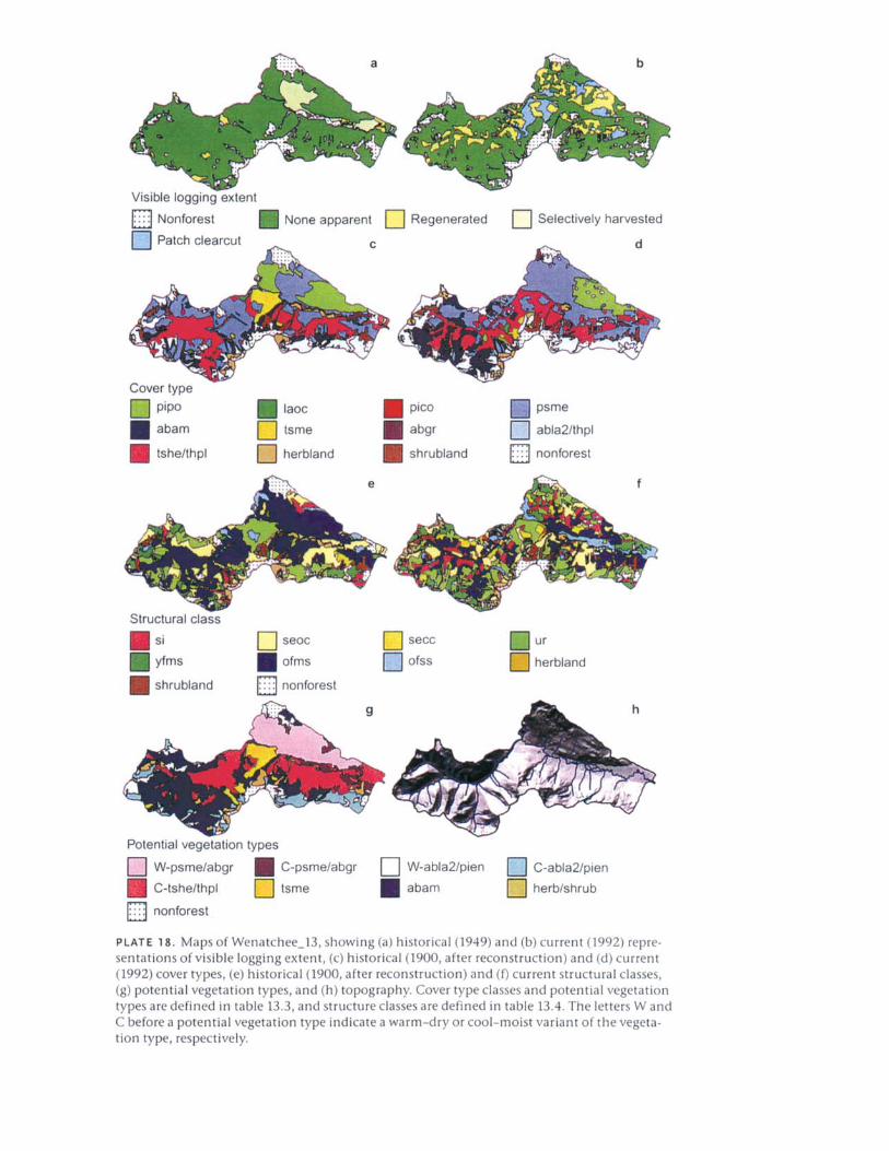
• Historical (1949, prior to reconstruction withmost-similar-neighbor analysis) and current(1992) visible logging extent (color plates 18aand b, respectively);

• Historical (after reconstruction with mostsimilar-neighbor analysis) and current covertypes (color plates 18c and d, respectively);

• Historical and current structural classes(color plates 18e and f, respectively);

story”; ofss, “old forest, single story”; Other, all non-forest and nonrangeland and anthropogenic types com-bined; secc, “stem exclusion, closed-canopy” seoc, “stemexclusion, open-canopy” Shrub, all shrubland covertypes and structural classes combined; si, stand initia-tion; ur, understory reinitiation; yfms, “young forest,multistory.”

2Totals may not add to 100% because of rounding errors.

• Potential vegetation types (color plate 18g);• Topography (color plate 18h);• Historical (after reconstruction with most-

similar-neighbor analysis) and current (1992)fuel loading (color plates 19a and b, respec-tively; and

• Historical and current crown fire potential(color plates 19c and d, respectively), flamelength (color plates 19e and f, respectively),and fireline intensity (color plates 19g and h,respectively) under an average wildfire scenario.

In the map of visible logging extent, selectioncutting had affected about 7.7% of the area. Se-lection cutting had a relatively minor influenceon structural conditions in the harvested areas,as fewer than half of the harvested “old forest,multistory” patches were sufficiently influencedto change their structural designation, and thosethat were affected were converted to “stem exclu-sion, open-canopy” or “old forest, single-story”structures. However, early selection cutting sig-nificantly modified cover types. Selection cuttingapparently targeted large overstory ponderosapine growing in the warm-dry and cool-moist


Douglas-fir (Pseudotsuga menziesii [Mirb.] Franco)/grand fir (Abies grandis [Dougl.] Lindl.) potentialvegetation types and converted much of the har-vested area to a Douglas-fir cover type. An addi-tional 23.7% of the current subwatershed areahas been influenced by timber harvesting, andthe most recent cutting has been patch clear-cutting to promote regeneration in the samepotential vegetation types.

The historical cover type and structural classmaps (color plates 18c,e) show simple, conta-gious patterns of land cover and forest structurereflecting the relatively simple patterns of po-tential vegetation types (color plate 18g) andtopography (color plate 18h). Both the simplepatterns and the high historical area of “old for-est, multistory” patches (38%, table 13.4) suggestthat fires have been infrequent in Wenatchee_13.The current logging extent, cover type, and struc-tural class maps (color plates 18b,d, and f, re-spectively) show a landscape fragmented into 49 regeneration units based on the type of har-vesting (minimum, 2.25 ha; maximum, 302 ha;median, 11.8 ha). A significant area of the pon-derosa pine cover type has been converted toDouglas-fir (4.6%), and 18% of the “old forest,multistory” area has been lost to the westernhemlock (Tsuga heterophylla [Raf.] Sarg.)-westernred cedar (Thuja plicata Donn), Douglas-fir, andponderosa pine cover types (see table 13.3).

Historical maps of fuel loading (color plate 19a),crown fire potential (color plate 19c), flamelength (color plate 19e), and fireline intensity(color plate 19g) depict a landscape that dis-played large contiguous areas with a very high(>30 Mg.ha-1) fuel loading and the potential forcrown fires under an average wildfire scenario,high to extreme flame lengths >6 m), and high to extreme fireline intensities (>1038 kW.m-1). It is evident from looking at the historical fuel(color plate 19a), fire behavior (color plate 19c),and structural class (color plate 19e) maps thatfires seldom burned in the Wenatchee_13watershed, but when they did, they were proba-bly significant: moderate severity fires with a large stand-replacement component (see table13.2, ESRLF). Current conditions suggest that pastmanagement activities in Wenatchee_13 havereduced the likelihood of stand-replacing fires,their attendant ecological effects, and the scalesof those effects.

EMDS Evaluation of Wenatchee_13

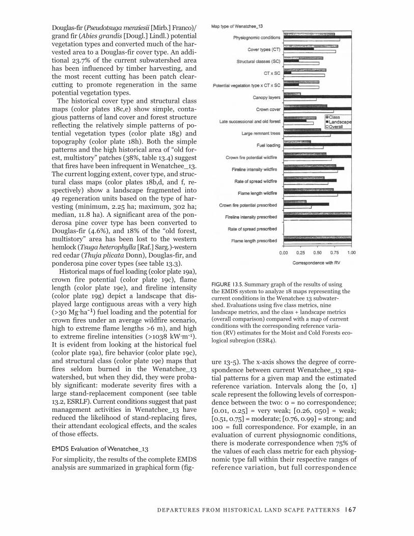
For simplicity, the results of the complete EMDSanalysis are summarized in graphical form (fig-

FIGURE 13.5. Summary graph of the results of using the EMDS system to analyze 18 maps representing thecurrent conditions in the Wenatchee 13 subwater-shed. Evaluations using five class metrics, nine landscape metrics, and the class + landscape metrics(overall comparison) compared with a map of currentconditions with the corresponding reference varia-tion (RV) estimates for the Moist and Cold Forests eco-logical subregion (ESR4).

ure 13-5). The x-axis shows the degree of corre-spondence between current Wenatchee_13 spa-tial patterns for a given map and the estimatedreference variation. Intervals along the [0, 1]scale represent the following levels of correspon-dence between the two: 0 = no correspondence;[0.01, 0.25] = very weak; [0.26, 050] = weak;[0.51, 0.75] = moderate; [0.76, 0.99] = strong; and100 = full correspondence. For example, in anevaluation of current physiognomic conditions,there is moderate correspondence when 75% ofthe values of each class metric for each physiog-nomic type fall within their respective ranges ofreference variation, but full correspondence


when 100% of the values for the landscape metrics fall within these ranges.

Evaluations of cover types

Evaluations of the current cover type conditionsshow strong overall correspondence; the corre-spondence is strong when the five class metricsare evaluated against estimates of reference vari-ation for all cover types, and weak when the ninelandscape metrics are evaluated (figure 13.5).Chief among the departures for the class metricsare the elevated patch densities for the Douglas-fir, grand fir, western hemlock-western red cedar,shrubland, and nonforest cover types. Weak cor-respondence between the current cover typemosaic and estimates of reference variation is a

result of elevated cover type richness, which isindicated by departures in patch richness anddiversity (table 13.5).

Physiognomic conditions

Physiognomic conditions show strong overallcorrespondence; correspondence was full whenlandscape metrics are evaluated, and moderatewhen class metrics are evaluated (figure 135)When we traced the basis of the latter conclusionin EMDS, we learned that the patch densities ofshrubland and nonforest and the edge density offorest (increased by the increased number of cutting units and their boundaries) are wellabove the limits of reference variation. Frag-mentation of forest cover types is so widespread


Notes: Corresponding reference variation (RV) and fullrange estimates developed for ESR4 B the Moist and ColdForests subregion are also shown. Values in bold lie out-side RV.

1CONTAG, contagion index; UI, interspersion and jux-taposition index (see also McGarigal and Marks 1995);

MSIEI, modified Simpson’s evenness index; N1, Hill’s N1index = eSHDI; N2, Hill’s N2 index = 1/SIDI; PR, patch rich-ness; R21, Alatalo’s evenness index = (N2 - 1)/(N1 - 1);RPR, relative patch richness; SHDI, Shannon diversityindex.

that it affected the edge density of the forestphysiognomy.

Structural Glass Conditions

Structural class conditions show only moderateoverall correspondence between current con-ditions and estimates of reference variation,moderate correspondence when class metrics areevaluated, and very weak correspondence whenthe landscape metrics are evaluated. Key depar-tures for the class metrics are the elevated patchdensity and reduced mean patch size. Weak correspondence between the current structuralclass mosaic and the estimates of reference vari-ation is a result of elevated diversity, dominance,evenness, interspersion, and juxtaposition ofstructural classes, and of dramatically reducedcontagion.

Combined cover type-structural class conditions

The combined map of cover type and structuralclass shows moderate overall correspondencebetween current conditions and estimates of reference variation; correspondence is moderatewhen class metrics are evaluated, and very weakwhen the landscape metrics are evaluated. Keydepartures for the class metrics are elevatedpatch densities and reduced mean patch sizes formost cover type-structural class combina-tions, but the mean nearest-neighbor distance isalso reduced for most classes. In addition, thereare departures in the percentage of total area inthe ponderosa pine, western larch (Larix occiden-taIis Nutt.), grand fir, and amabilis fir (Abies am-nbilis [Dougl.] Forbes) stand-initiation structures,representing an expanded area of new forest,and in intermediate forest structures (“stem ex-clusion, open-canopy,” “stem exclusion, closedcanopy,” and “young forest, multistory”) associ-ated with the ponderosa pine, grand fir, andwestern hemlock-western red cedar cover types.

Weak correspondence between the currentcombined cover type-structural class mosaic andthe estimates of reference variation is a result ofincreased richness, diversity, dominance, even-ness, interspersion, and juxtaposition of struc-tural class patches and of reduced contagion.The combined potential vegetation type-covertype-structural class mosaic shows nearly iden-tical results (figure 13.5).

Fragmented landscapes

The common finding among each of the 18 mapevaluations is that the landscape had becomehighly fragmented, an observation that is consis-

tently indicated by reduced contagion, elevatedpatch densities and mean nearest-neighbor dis-tances, and reduced mean patch sizes. Nowhereis this better indicated than in the evaluations offuel loading, crown fire potential, and fire be-havior patterns. For example, fuel loading showsmoderate overall correspondence between cur-rent conditions and estimates of reference vari-ation; correspondence is full when landscapemetrics are evaluated, and weak when class metrics are evaluated. When we traced the basisof the conclusions in EMDS, we learned thatpatch density and mean patch size in all fuelloading classes are well outside of the referencevariation (color plate 19b).

Departures in Landscape Patterns forWenatchee_13

Reduced area of old forest

Tables 13.3 and 13.4 display all cover type andstructural class transitions from the historical tothe current conditions. Early selection cuttingapparently targeted large, easily accessed over-story ponderosa pine growing in warm-dry and cool-moist Douglas-fir-grand fir potentialvegetation types, and large overstory Douglas-fir growing in cool-moist western hemlock-western red cedar and amabilis fir potential veg-etation types. Most of the recent regenerationcutting has been in the same environments.Analysis of the transitions from historical to current structural classes (see table 13.4) showsa net IS% reduction in “old forest, multistory”structures and corresponding increases in standinitiation (6.9%), “stem exclusion, open-canopy”(3.9%), “stem exclusion, closed-canopy” (2.2%),understory reinitiation (4.9%), and “young for-est, multistory” (3.0%) structures.

Reduced cover of large, early seral overstory trees

Similarly, analysis of the transitions from histor-ical to current cover types (see table 13.3) showsa net 3.7% reduction in the ponderosa pine covertype and an increase (4.6%) in the Douglas-fircover type. A combined cover type-structuralclass transition analysis showed a total transitionof large, early seral overstory Douglas-fir coverequal to 11.7% of the subwatershed area to lateseral cover comprising amabilis fir (3.6%), grandfir (0.5%), alpine fir (Abies lasiocarpa [Hook.]Nutt.)-Engelmann spruce (Picea engelmanniiParry) (2.4%), and western hemlock-western redcedar (5.2%) understory cover types. This transi-tion can also be seen in table 13.3, and it reflects


the removal of large Douglas-fir overstories from“old forest, multistory” patches.

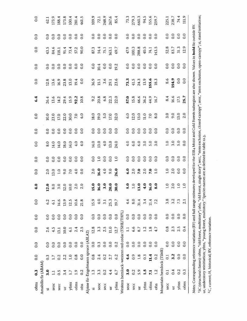
In table 13.6, we compare current and histori-cal values of three class metrics (percentage oftotal area, patch density, and mean patch size)for a partial list of cover type-structural classcombinations with corresponding estimates ofreference variation. For example, the estimatedpercentage area of the ponderosa pine stand-initiation class is 0.0-1.1% of the total area. Inthe current condition, this class occupies 1.4% ofthe area, and the current area is above the es-timates for reference variation. This increaseddominance of ponderosa pine stand-initiationstructures resulted from regeneration harvests.

Also in table 13.6, we display historical valuesof the class metrics and the full range of histori-cal values for each class and metric. Significanthistorical and current departures from referencevariation are highlighted in bold. Class metricsfor several current and historical cover type-structural class combinations lie outside the esti-mated reference variation. Structural classes ofthe ponderosa pine, Douglas-fir, and westernhemlock-red cedar cover types exhibit the great-est departures, because these classes contain thegreatest area of “old forest, multistory” structures,and old forests were targeted for early selectioncutting, and more recently, for regeneration har-vests (Hessburg et al. 1999b; Hessburg and Ageein press) (see tables 13.3, 13.4) In the historicalcondition, there was no area of “stem exclusion,closed canopy” or understory reinitiation patchesin the ponderosa pine cover type, and the area in“young forest, multistory” patches was small(0.2%). A likely explanation is that historicalsurface fires and dry site conditions on sites withsouthern aspects maintained open-canopy ratherthan closed-canopy stem-exclusion structures(Agee 1993). The net effect was a simplified land-scape mosaic on lower montane sites with south-ern aspects; ponderosa pine land cover was his-torically dominated by “old forest, multistory”and “old forest, single story” structures, andtrace amounts of stand initiation, “stem exclu-sion, open canopy,” and “young forest, multi-story” structural classes (see tables 13.4, 13.6).

Working with unique or borderline watersheds of a subregion

The estimates of reference variation for areas of ponderosa pine, Douglas-fir, and westernhemlock-western red cedar “old forest, multi-story” patch types ranged, respectively, from 0%to 2.3, 12.5, and 1.8%, but the historical areas of

these structures were 8.5, 16.9, and 11.41 respec-tively; these values lie well above the estimatedrange of reference variation. Wenatchee_13 issomewhat unusual among the historical sub-watersheds we sampled because 38% of thewatershed comprised “old forest, multistory”structures (see table 13.4) and this area was ag-gregated in a few large patches (table 13.6). Thisobservation suggests that it may be appropriateto consider the full range of values for the classand landscape metrics when evaluating opportu-nities to restore the area, connectivity, and pat-tern of old forests and perhaps other attributes ofsome Moist and Cold Forest subregion land-scapes. Unique fire ecology, landform features, orenvironments may make some landscapes of asubregion appear atypical. We discuss some rea-sons for this in our Conclusions section.

Relevance of Departures in Landscape Patterns

At relatively fine to broad spatial and temporalscales, the response of terrestrial species to land-scapes and their patterns indicates whether theseenvironments are more or less suitable to theirparticular needs. Changes in the patterns of veg-etation at certain spatial and temporal scalesmay have a direct bearing on species migration,colonization, the availability of habitats andfood, and the persistence of a species in a land-scape (Wisdom et al. 2000). As patterns changesignificantly, different suites of species may befavored. Such changes also influence the spatialand temporal scales and parameters of distur-bance regimes. As tables 13.5 and 13.6 show,variability in the spatial patterns of historicallandscapes was commonplace. Variable land-scape patterns at subwatershed, watershed, sub-regional, and regional scales probably providealternating periods and patterns of plenty andneed that may help native species to developbroad genetic and phenotypic diversity and nec-essary adaptations as long as habitats do notbecome overly fragmented or isolated in space ortime (Swanson et al. 1994). Natural variability invegetation patterns, climate, and geological sys-tems is also linked to natural variation in distur-bance regimes.

After evaluating the classes in the 18 mapswith respect to reference variation, we character-ized departures in spatial patterns for each land-scape mosaic. For example, we compared theoverall current cover type-structural class mosaicof Wenatchee_13 with corresponding estimatesof reference variation (table 13.5). Current valuesof eight of the nine landscape metrics lie beyond


these limits; historical values of five metrics alsoshow evidence of departures. In the We-natchee_13 historical condition, all richness and diversity metrics are above the estimates ofreference variation for the subregion. Thus We-natchee_13, at least in this temporal snapshot,displayed a richer and more diverse array of covertype-structural class patches than ordinarily oc-curred in similar subwatersheds of the subregionin the period for which we characterized refer-ence variation. This was probably true of otherwatersheds and landscape attributes at othertimes. In the historical condition, Wenatchee_13displayed nearly 47% of the total possible num-ber of cover type-structural class combinationsthat were present in the entire subregion (rela-tive patch richnesshistorical; table 13.5); in the

current condition, more than 55% of those pos-sibilities are displayed. The historical value ofabsolute patch richness exceeds the estimatedreference variation by more than four covertype-structural class patch combinations, andseven cover type-structural class combinationsdeveloped in the landscape as a consequence ofmanagement activities.

In the historical Wenatchee_13, three indicesregistered as lying above the reference variation:Shannon’s diversity index, which measures theproportional abundance of classes and the equi-table distribution of area; N1, a transformationof Shannon’s diversity index; and N2, the in-verse of Simpson’s lambda, a metric that repre-sents dominance and diversity. Current valuesfor the three metrics also lie above the limits ofthe full range of variation. Timber harvestingcoupled with fire exclusion has created manynew cover type-structural class combinations.For example, a comparison of historical and cur-rent values of N2 indicates that the number ofdominant cover type-structural class combina-tions increased from about 14 to 25 (table 13.5).

A comparison of the historical and currentvalues of the evenness metrics (modified Simp-son’s evenness index and Alatalo’s R21 evennessindex) shows significantly elevated evennessamong the cover type-structural class combina-tions. The modified Simpson’s index is sensitive tochanges in the evenness of all classes, in-cluding rare ones; Alatalo’s index is sensitive tochanges in the evenness of the dominant classes.Harvesting activities increased the complexityand evenness of patterns in the cover type-structural class mosaic. Considering only thedominant 25 cover type-structural class combi-nations (N2current), the current mosaic displays

9o% of the maximum possible evenness for thenumber of classes in the subregion (R2current).

The historical mosaic displays 73% of the maxi-mum possible evenness (table 13.5).

The current value of the contagion metric alsolies outside the range of the estimates of refer-ence variation, but unlike other landscape met-rics, contagion decreased when compared withits historical value. Contagion was apparentlyreduced by timber harvesting (color plate 18b)and perhaps by fire exclusion, which fragmentedthe historical areas of “old forest, multistory”structures. Timber harvests had homogenized thesimple, contagious patterns of forest structure inthe historical landscape.

Conclusions

A scientific and social consensus is emergingthat land managers must restore more naturalconditions to forests. One approach focuses man-agement and restoration efforts on emulatingnatural disturbance, but restoring the role of dis-turbance requires to some extent emulation ofthe range and variation in the vegetation condi-tions that support it. Before settlement of the re-gion, fire played a dominant role in sculptingvegetation patterns and the associated pro-cesses. Before restoring the natural role of dis-turbance, managers must restore more naturalvariation in the spatial and temporal patterns ofvegetation.

We estimated reference variation conserva-tively so as to define an approximate range ofecologically justifiable conditions (e.g., Landreset al. 1999; Parsons et al. 1999; Swetnam et al. 1999)and to identify ecologically important changes in pattern features (e.g., extents and patterns ofold forest or early seral species). When preparingrestoration prescriptions,. reference conditionsshould be used as a general rather than a rigidguide, and restored landscapes should reflectbroad variation in patterns rather than the modalconditions.

Our selection of a range statistic was arbitrary;other variance measures could be used. We usedthe median because the right-skewed distribu-tions of reference variation required a measureof central tendency that defined a representativerange of conditions. We excluded extremes bynot using the full range of variation.

The sampling method used to define the ref-erence conditions substitutes space for time.Broad sampling of spatial patterns of vegeta-tion from similar environments with similar disturbance and climatic regimes should reveal a


representative cross section of temporal varia-tion in these patterns (Pickett 1989). In effect,variation observed over broad spaces and narrowtimes may be as effective as observing variationover broad times and narrow spaces; both let usinfer variations in spatial pattern at a single lo-cation or across a single landscape over time.Particularly when we try to explain the influenceof processes, sampling locations must have comparable biophysical and climatic conditions(Pickett 1989). We addressed this concern by strat-ifying our reconstructed historical subwatershedsinto subregions with similar climate, geology,biology, and disturbance regimes. The remain-ing potential pitfalls include an inadequate timedepth, locally incompatible disturbance and cli-mate histories, convergent environmental his-tories, and nonhomogeneous environments.

Comparing current values of spatial patternmetrics with estimates of reference variation re-veals ecologically important departures. Compar-ing historical values with these estimates revealsunique landscapes or landscape conditions thatlie outside the typical reference conditions. Atyp-ical cases should be frequent, because region-alizations define homogeneous ecoregions; inreality, these overlap somewhat, and each re-sembles neighboring ecoregions to some extent(e.g., see Hessburg et al. 2000a). It is difficult tomap intergradations between the cores of eco-regions, where atypical landscapes and patternsoften appear. To minimize this problem, we an-alyzed reference variation, but the full range ofconditions could be used to evaluate apparentlyatypical conditions.

Regionally synchronous weather or distur-bance (convergent environmental histories),which are often related, would simplify esti-mates of a region’s reference variation. For thisreason, estimates should ultimately include vari-ations resulting from stochastic features and rareevents. This can be done by temporally and spa-tially broadening samples where data are avail-able and by process modeling (e.g., Keane et al.2002b, chapter 5, this volume), in which simu-lated vegetation conditions contribute to com-puting reference variation. We simulated vege-tation and disturbance conditions in a few ecoregions and found that estimates such asthose presented in this chapter correspond rea-sonably well with the simulated results. How-ever, the possibility for errors or uncertainties inthe spatial data remains, and can lead to estima-tion and prediction errors.

Managers can use our approach to perform similar evaluations elsewhere. To do so, it is es-sential to associate estimates of reference vari-ation with specific potential vegetation types,because distributions of cover type-structuralclass combinations vary significantly; fire, in-sect, and pathogen disturbances, which accountfor much of the natural variation in vegetationspatial patterns, strongly correlate with the en-vironmental setting (Pickett and White 1985).Hessburg et al. (1999b) illustrated how referencevariation can be computed for potential vege-tation type-cover type-structural class combi-nations and how that information can identifybiophysical environments and guide revisions tocover type-structural class patterns.

Empirical estimates of reference variation serveseveral useful functions. Managers can use themto:• Evaluate current conditions and estimate

potential consequences for native species andprocesses (Morgan et al. 1994; Landres et al.1999);

• Assess scenarios that differ from referenceconditions and evaluate the potential op-portunities and risks for native species,processes, and ecosystem productivity;Develop and evaluate specific restorationgoals (Allen et al. 2002);

• Develop strategies and conservation andrestoration priorities at multiple geographicscales; and

• Monitor progress in ecosystem managementat relevant geographic scales.

A decision-support system, such as EMDS, canautomate landscape evaluations at several scales.At a regional scale, fully integrated knowledgebases can represent reference conditions for sub-regions. Landscape evaluations can reveal sub-regions that contain the land areas with impor-tant or extensive departures from natural rangesand thereby guide the strategic allocation of plan-ning and restoration resources (e.g., Reynoldsand Hessburg 2004). At a Subregional scale, eval-uating a few critical attributes of all watershedscan identify priorities for more complete evalua-tion. At a subwatershed or landscape scale, eval-uations, such as the one in this chapter, can helpmap alternative restoration scenarios and con-trast them with estimates of reference variationbefore choosing and implementing the mostsuitable approach.



Acknowledgments

The Sustainable Management Systems Programof the U.S. Department of Agriculture ForestService’s Pacific Northwest Research Stationprovided financial support for this study. The

authors thank Dave W. Peterson, Jim Agee, EdDepuit, and three anonymous reviewers for their helpful comments and reviews of earlierdrafts.

emulating natural forest landscape disturbances

Documents