Economic Modelling 29 (2012) 2583–2590

Contents lists available at SciVerse ScienceDirect

Economic Modelling

j ourna l homepage: www.e lsev ie r .com/ locate /ecmod

Empirical mode decomposition–based least squares support vector regression forforeign exchange rate forecasting

Chiun-Sin Lin a, Sheng-Hsiung Chiu b, Tzu-Yu Lin b,⁎a Department of Business and Entrepreneurial Management, Kainan University, No.1 Kainan Road, Luzhu Shiang, Taoyuan 33857, Taiwanb Department of Management Science, National Chiao Tung University, No. 1001, Ta-Hsueh Road, Hsinchu City 30010, Taiwan

⁎ Corresponding author. Tel.: +886 921865025.E-mail address: blackmallows@gmail.com (T.-Y. Lin)

0264-9993/$ – see front matter © 2012 Elsevier B.V. Allhttp://dx.doi.org/10.1016/j.econmod.2012.07.018

a b s t r a c t

a r t i c l e i n f o

Article history:Accepted 11 July 2012

Keywords:Empirical mode decompositionLeast-squares support vector regressionForeign exchange rate forecastingIntrinsic mode function

To address the nonlinear and non-stationary characteristics of financial time series such as foreign exchangerates, this study proposes a hybrid forecasting model using empirical mode decomposition (EMD) and leastsquares support vector regression (LSSVR) for foreign exchange rate forecasting. EMD is used to decomposethe dynamics of foreign exchange rate into several intrinsic mode function (IMF) components and one residualcomponent. LSSVR is constructed to forecast these IMFs and residual value individually, and then all these fore-casted values are aggregated to produce the final forecasted value for foreign exchange rates. Empirical resultsshow that the proposed EMD-LSSVR model outperforms the EMD-ARIMA (autoregressive integrated movingaverage) as well as the LSSVR and ARIMA models without time series decomposition.

© 2012 Elsevier B.V. All rights reserved.

1. Introduction

Financial time series forecasting has come to play an importantrole in the world economy as a result of its ability to forecast economicbenefits and influence countries' economic development; it hasattracted increasing attention from academic researchers and businesspractitioners for its theoretical possibilities and practical applications(Hadavandi et al., 2010; Lu et al., 2009). Since the breakdown of finan-cial market boundaries in order to enhance the efficiency of capitalfunding, for example, the Bretton Woods system of monetary manage-mentwas officially ended in the 1973; currencies traded internationallyhas become crucial economic indices for international trade, financialmarkets, the alignment of economic policy by governments, and corpo-rate financial decision-making. However, it is widely known that finan-cial time series forecasting has shortcomings, including its inherentnonlinearity and non-stationarity (Huang et al., 2010; Lu et al., 2009).Therefore, financial time series forecasting is one of the most challeng-ing tasks in the financial markets.

For modeling financial time series, autoregressive integratedmoving average (ARIMA) models have been popular and are widelychosen for academic research observing the behavior of foreignexchanges and stock markets, because of their statistical propertiesand forecasting performance (Khashei et al., 2009). However, someproblems arise when forecasting financial time series with ARIMAmodels, as follows. First is the characteristic linear limitation of ARIMAmodels, in contrast to real-word financial time series, which are often

.

rights reserved.

nonlinear (Khashei et al., 2009; Zhang, 2001; Zhang et al., 1998) andare rarely pure linear combinations. Second is the robustness limitationof ARIMA models—the ARIMA model selection procedure dependsgreatly on the competence and experience of the researchers to yielddesired results. Unfortunately, choice among competing models canbe arbitrated by similar estimated correlation patterns and may fre-quently reach inappropriate forecasting results.

With the recent development of machine-learning algorithms,several methods have been utilized that work more effectively thanthe traditional linear model in time series forecasting problems. Forexample, the support vector machine (SVM) is a novel machine-learning approach. SVM's generalization capability in obtaining aunique solution (Lu et al., 2009) and structural risk minimizationprinciple (SRM) in achieving high performance (Duan and Stanley,2011) have drawn attention to SVM's research applications. Supportvector regression (SVR) is the regression model of SVM (Vapnik,2000). It has been applied to investigate the forecasting ability of finan-cial time series. Lu et al. (2009) used SVR to construct a stock price fore-casting model, and Huang et al. (2010) and Ni and Yin (2009) bothimplemented SVR in exchange rate forecasting models. However,the training phrase of SVR is a time-consuming process when thereis a lot of data to deal with. Therefore, least squares support vectorregression (LSSVR), proposed by Suykens and Vandewalle (1999),has been applied in much literature as an alternative (He et al., 2010;Khemchandani et al., 2009); it is a simplified version of traditionalSVR that alters inequality constraints into equal conditions and employsa squared loss function, which is a differential setting relative to tradi-tional SVR (Wang et al., 2011), to achieve higher calculation speedand efficiency while retaining the advantage of the structural risk min-imization principle.

2584 C.-S. Lin et al. / Economic Modelling 29 (2012) 2583–2590

When we model financial time series using LSSVR or ARIMA, wemust remember that these financial time series are inherentlynonlinear and non-stationary. If we ignore this problem, it will resultinworse forecasting. The property offinancial time series and the divideand conquer principle (Yu et al., 2008) are important in constructing afinancial time series forecasting model. Therefore, hybrid models arewidely used to solve the limitations in financial time series forecasting.Empirical mode decomposition (EMD) is suitable for financial timeseries in terms of finding fluctuation tendency, which simplifies theforecasting task into several simple forecasting subtasks. EMD as atime–frequency resolution approach offers a new way by which the-stationary and nonlinear behavior of time series can be decomposedinto a series of valuable independent time resolutions (Tang et al.,2012). It also can reveal the hidden patterns and trends of time series,which can effectively assist in designing forecasting models for variousapplications (An et al., 2012; Guo et al., 2012). Guo et al. (2012), for ex-ample, decomposed wind-speed series using EMD and then forecastedthem using a feed-forward neural network, whereas Chen et al.(2012) proposed an EMD approach combined with an artificial neuralnetwork for tourism-demand forecasting.

In this paper, EMD and LSSVR are used to present a financial timeseries forecasting model for foreign exchange rate, in which consider-ation of the decomposed financial time series structure will increasethe accuracy and practicability of the proposed model in terms of over-coming the nonlinearity and non-stationarity limitations to the linearstatistical model. The proposed approach is compared with the com-bination of EMD and ARIMA as well as with the existing LSSVR andARIMA models, and it is shown that the proposed model can yieldmore accurate results. Three financial time series are used as illustrativeexamples, as follows: USD/NTD exchange rate, JPY/NTD exchange rate,and RMB/NTD exchange rate.

2. Methodology

2.1. Empirical mode decomposition

Empirical mode decomposition (EMD) is a nonlinear signal-transformation method developed by Huang et al. (1998, 1999). It isused to decompose a nonlinear and non-stationary time series intoa sum of intrinsic mode function (IMF) components with individualintrinsic time scale properties. According to Huang et al. (1998),each IMF must satisfy the following two conditions. First, the number

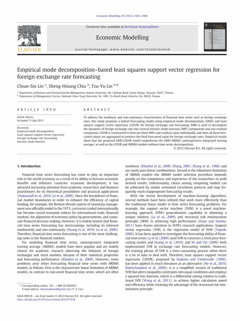
Foreign ExchaData

EMD

IMF1 IMF2 IMFn...

SVR1 SVR2 SVRn...

Prediction R

Fig. 1. The proposed EMD-LSSVR forecast

of extreme values and zero-crossings either are equal or differ at themost by one; and second, the mean value of the envelope constructedby the local maxima and minima is zero at any point. The detail-decomposition process of EMD is presented by Huang et al. (1998).Suppose that a data time series can be decomposed according to the fol-lowing procedure.

(1) Identify all the local maxima and minima of x(t).(2) Obtain the upper envelope xu(t) and the lower envelope xl(t)

of the x(t).(3) Use the upper envelope xu(t) and the lower envelope xl(t) to

compute the first mean time series m1(t), that is, m1(t)=[xu(t)+xl(t)]/2.

(4) Evaluate the difference between the original time series x(t) andthe mean time series and get the first IMF h1(t), that is, h1(t)=x(t)−m1(t).Moreover,we seewhetherh1(t) satisfies the two con-ditions of an IMF property. If they are not satisfied, we repeat steps1–3 of the decomposition procedure to eventually find the firstIMF.

(5) After we obtain the first IMF, a repeat of the above steps is neces-sary to find the second IMF, until we reach the final time seriesr(t) as a residue component that becomes a monotonic function,which is suggested for stopping the decomposition procedure(Huang et al., 1999).

The original time series x(t) can be reconstructed by summing upall the IMF components and one residue component as Eq. (1), asfollows.

x tð Þ ¼Xni¼1

hi tð Þ þ r tð Þ: ð1Þ

2.2. Least squares support vector regression

The support vector machine (SVM) developed by Vapnik (1995,2000) is based on the SRM principle. It aims to minimize the upperbound of the generalization error, instead of the empirical error as inother neural-network methods such as back-propagation networks(BPN). SVM explores not only the problem of classification but also theregression application of forecasting. Vapnik et al. (1997) proposed sup-port vector regression (SVR) as an SVM regression estimation model,introducing the concept of the ε-loss function.

nge Rate

-1 IMFn R n

-1 SVRn SVRn+1

esults

Input

Outputput

ing model for foreign exchange rate.

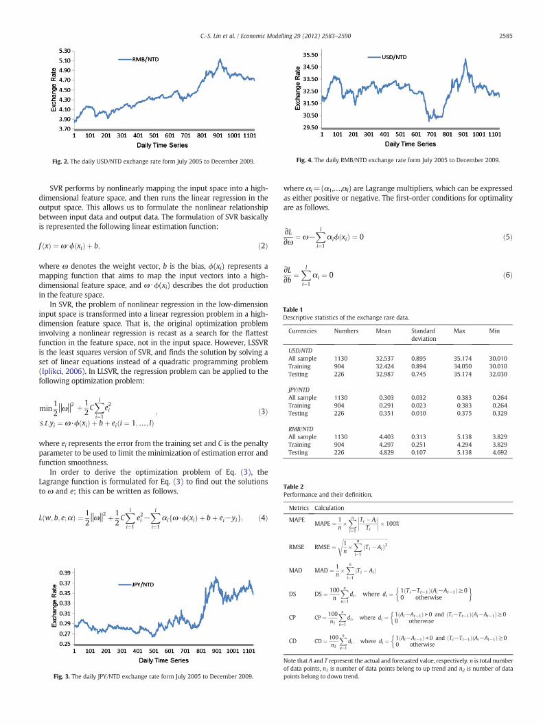
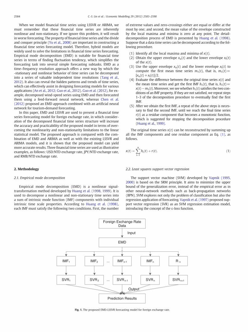
Fig. 2. The daily USD/NTD exchange rate form July 2005 to December 2009. Fig. 4. The daily RMB/NTD exchange rate form July 2005 to December 2009.

Table 1Descriptive statistics of the exchange rare data.

Currencies Numbers Mean Standarddeviation

Max Min

USD/NTDAll sample 1130 32.537 0.895 35.174 30.010Training 904 32.424 0.894 34.050 30.010Testing 226 32.987 0.745 35.174 32.030

JPY/NTDAll sample 1130 0.303 0.032 0.383 0.264Training 904 0.291 0.023 0.383 0.264Testing 226 0.351 0.010 0.375 0.329

RMB/NTDAll sample 1130 4.403 0.313 5.138 3.829Training 904 4.297 0.251 4.294 3.829Testing 226 4.829 0.107 5.138 4.692

Table 2Performance and their definition.

Metrics Calculation

MAPEMAPE ¼ 1

n�Xni¼1

Ti � Ai

Ti

��������� 100%

2585C.-S. Lin et al. / Economic Modelling 29 (2012) 2583–2590

SVR performs by nonlinearly mapping the input space into a high-dimensional feature space, and then runs the linear regression in theoutput space. This allows us to formulate the nonlinear relationshipbetween input data and output data. The formulation of SVR basicallyis represented the following linear estimation function:

f xð Þ ¼ ω⋅ϕ xið Þ þ b; ð2Þ

where ω denotes the weight vector, b is the bias, ϕ(xi) represents amapping function that aims to map the input vectors into a high-dimensional feature space, and ω⋅ϕ(xi) describes the dot productionin the feature space.

In SVR, the problem of nonlinear regression in the low-dimensioninput space is transformed into a linear regression problem in a high-dimension feature space. That is, the original optimization probleminvolving a nonlinear regression is recast as a search for the flattestfunction in the feature space, not in the input space. However, LSSVRis the least squares version of SVR, and finds the solution by solving aset of linear equations instead of a quadratic programming problem(Iplikci, 2006). In LLSVR, the regression problem can be applied to thefollowing optimization problem:

min12‖ω‖2 þ 1

2CXli¼1

e2i

s:t:yi ¼ ω·ϕ xið Þ þ bþ ei i ¼ 1;…; lð Þ; ð3Þ

where ei represents the error from the training set and C is the penaltyparameter to be used to limit the minimization of estimation error andfunction smoothness.

In order to derive the optimization problem of Eq. (3), theLagrange function is formulated for Eq. (3) to find out the solutionsto ω and e; this can be written as follows.

L w; b; e;αð Þ ¼ 12‖ω‖2 þ 1

2CXli¼1

e2i −Xli¼1

αi ω·ϕ xið Þ þ bþ ei−yif g; ð4Þ

Fig. 3. The daily JPY/NTD exchange rate form July 2005 to December 2009.

where αi=(α1,…,αl) are Lagrange multipliers, which can be expressedas either positive or negative. The first-order conditions for optimalityare as follows.

∂L∂ω ¼ ω−

Xli¼1

αiϕ xið Þ ¼ 0 ð5Þ

∂L∂b ¼

Xli¼1

αi ¼ 0 ð6Þ

RMSE RMSE ¼ffiffiffiffiffiffiffiffiffiffiffiffiffiffiffiffiffiffiffiffiffiffiffiffiffiffiffiffiffiffiffiffiffiffiffiffiffi1n�Xni¼1

Ti � Aið Þ2s

MAD MAD ¼ 1n�Xni¼1

Ti � Aij j

DS DS ¼ 100n

Xnu¼1

di; where di ¼ 1 Ti−Tt−1ð Þ Ai−At−1ð Þ≥00 otherwise

� �

CP CP ¼ 100n1

Xnu¼1

di; where di ¼ 1 AI−At−1ð Þ≻0 and Ti−Tt−1ð Þ Ai−At−1ð Þ≥00 otherwise

�

CD CD ¼ 100n2

Xnu¼1

di; where di ¼ 1 AI−At−1ð Þ≺0 and Ti−Tt−1ð Þ Ai−At−1ð Þ≥00 otherwise

�

Note that A and T represent the actual and forecasted value, respectively. n is total numberof data points, n1 is number of data points belong to up trend and n2 is number of datapoints belong to down trend.

2586 C.-S. Lin et al. / Economic Modelling 29 (2012) 2583–2590

∂L∂ei

¼ C·ei−αi ¼ 0 ð7Þ

∂L∂αi

¼ ω·ϕ xið Þ þ bþ ei−yi ¼ 0: ð8Þ

By solving the above linear system, the forecasting formulation ofLSSVR can be represented in the following equation:

f xð Þ ¼Xli¼1

αiK xi; xj� �

þ b; ð9Þ

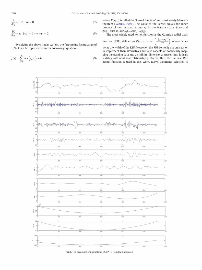
Fig. 5. The decomposition results for

where K(xi,xj) is called the “kernel function” andmust satisfy Mercer'stheorem (Vapnik, 1995). The value of the kernel equals the innerproduct of two vectors, xi and xj, in the feature space ϕ(xi) andϕ(xj); that is, K(xi,xj)=ϕ(xi)⋅ϕ(xj).

The most widely used kernel function is the Gaussian radial basis

function (RBF), defined as K xi; xj� ¼ exp

−‖xi−xj‖2

2σ2

!, where σ de-

notes the width of the RBF. Moreover, the RBF kernel is not only easierto implement than alternatives, but also capable of nonlinearly map-ping the training data into an infinite-dimensional space; thus, it dealssuitably with nonlinear relationship problems. Thus, the Gaussian RBFkernel function is used in this work. LSSVR parameter selection is

USD/NTD from EMD approach.

2587C.-S. Lin et al. / Economic Modelling 29 (2012) 2583–2590

most important, so that we can see that the established LLSVR modelwith Gaussian RBF kernel function goes well, because these parameterscan significantly affect generalized performance. Grid search (He et al.,2010), one of the most useful methods for parameter optimization,is applied to find the optimal parameters, C and σ, in LSSVR modelconstruction.

3. Proposed EMD-LSSVR model

Many studies have used least squares support vector regression inpractice problems (Khemchandani et al., 2009; Lin et al., in press). Infinancial time series forecasting, however, the major problems are inher-ent nonlinearity and non-stationary properties affecting the robustness of

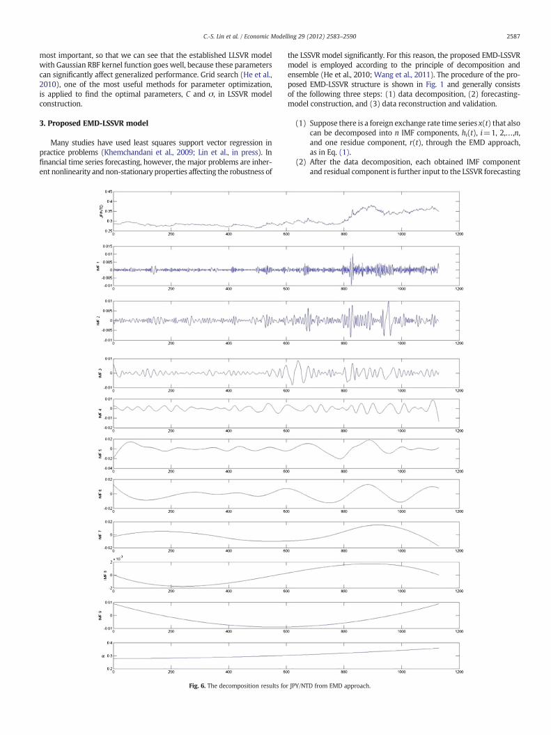
Fig. 6. The decomposition results fo

the LSSVR model significantly. For this reason, the proposed EMD-LSSVRmodel is employed according to the principle of decomposition andensemble (He et al., 2010; Wang et al., 2011). The procedure of the pro-posed EMD-LSSVR structure is shown in Fig. 1 and generally consistsof the following three steps: (1) data decomposition, (2) forecasting-model construction, and (3) data reconstruction and validation.

(1) Suppose there is a foreign exchange rate time series x(t) that alsocan be decomposed into n IMF components, hi(t), i=1, 2,…,n,and one residue component, r(t), through the EMD approach,as in Eq. (1).

(2) After the data decomposition, each obtained IMF componentand residual component is further input to the LSSVR forecasting

r JPY/NTD from EMD approach.

2588 C.-S. Lin et al. / Economic Modelling 29 (2012) 2583–2590

model; consequently, the corresponding forecasted values for allIMF and residual components are acquired from the forecastingtool.

(3) The forecasted value of each IMF and residual component in theprevious stage can be reconstructed as a sum of superposition ofall components, which can be used as the final forecasting result,and then compared with the original time series according toseveral criteria for measuring the performance capability of thisproposed model.

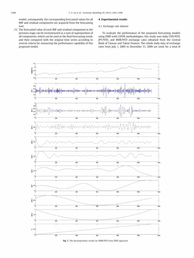
Fig. 7. The decomposition results for

4. Experimental results

4.1. Exchange rate dataset

To evaluate the performance of the proposed forecasting modelsusing EMD with LSSVR methodologies, this study uses daily USD/NTD,JPY/NTD, and RMB/NTD exchange rates obtained from the CentralBank of Taiwan and Yahoo Finance. The whole daily data of exchangerates from July 1, 2005 to December 31, 2009 are used, for a total of

RMB/NTD from EMD approach.

Table 4The parameter selection of single LSSVR forecasting model.

Kernel USD/NTD JPY/NTD RMB/NTD

RBF C σ C σ C σ64 0.25 64 0.125 64 0.0312

Table 5The exchange rate forecasting results using EMD-LSSVR, EMD-ARIMA, LSSVR andARIMA models.

Models Indicators

2589C.-S. Lin et al. / Economic Modelling 29 (2012) 2583–2590

1130 data points, as illustrated in Figs. 2–4 for each of the three ratesrespectively. These datasets are also divided into training group andtesting group in separate foreign exchange rate categories. The first904 data points (80% of the total dataset) are used as the traininggroup and the remaining 226 data points are used as the testinggroup. Table 1 shows some basic summary statistics for total, training,and testing data within the three foreign exchange rate datasets.

4.2. Performance criteria

Following Lu et al. (2009) and Tay and Cao (2001), the followingperformance measures are used and evaluated respectively: appliedmean absolute percentage error (MAPE), root‐mean‐square error(RMSE), mean absolute difference (MAD), directional symmetry(DS), correct uptrend (CP), and correct downtrend (CD) for consider-ation. The definition of these criteria can be summarized in Table 2.MAPE, RMSE, and MAD are measures of the deviation between theactual and forecasted value. They can be used to evaluate forecastingerror. The smaller the values of the criteria, the closer the forecastedvalue to the actual value. DS provides the correctness of the forecasteddirection of the exchange rate in terms of percentage, while CP andCD provide the correctness of the forecasted up trend and down trendsof exchange rate, also in terms of percentage. DS, CP, and CD can be uti-lized to provide forecasting accuracy.

4.3. Forecasting results

In this section, the forecasting results of the EMD-LSSVR model arecompared to those of other linear and nonlinearmodels. First is anotherhybrid forecasting model, one that integrates EMD with ARIMA. EMDis applied to decompose the foreign exchange rate time series, andgathered components that have a monotonic function, enhancing theforecasting ability of LSSVR and ARIMA. The others are the singleLSSVR and ARIMA models without algorithms or treatments for fore-casting. That is, the single LSSVR and ARIMA model were directly ap-plied to forecast future exchange rates. The purpose of doing so is toexplore the problem of financial time series forecasting based on linearand nonlinearmodels, whether we can preprocess forecasting variablesusing the EMD approach or not, thus helping to further managerialapplications.

The modeling steps of the proposed EMD-LSSVR are shown inSection 3. Using the EMD approach in the data decomposition, thethree foreign exchange rate time series can be decomposed into nineindependent IMFs and one residue component, respectively, as illus-trated in Figs. 5–7. These decomposition results may enhance themodel's forecasting ability in terms of the divide and conquer concept(Yu et al., 2008). Then, the decomposed forecasting variables, the inde-pendent IMFs, and residual components from the previous step, areused in LSSVR model construction. Parameter selection is essential forLSSVR model construction; we employ the Gaussian RBF as the kernel

Table 3The parameter selection of EMD-LSSVR forecasting model.

Kernel USD/NTD JPY/NTD RMB/NTD

RBF Set C σ Set C σ Set C σ

1 0.5 0.00390625 1 8 0.00390625 1 0.5 0.0156252 64 1 2 1 0.00390625 2 0.5 0.003906253 64 1 3 64 0.5 3 1 0.00781254 16 0.5 4 64 0.5 4 64 15 64 1 5 64 1 5 32 16 64 1 6 64 1 6 64 17 64 1 7 64 1 7 32 18 64 1 8 64 1 8 64 19 64 1 9 64 0.015625 9 32 0.2510 64 1 10 64 1 10 64 1

function of LSSVR. The parameter combination (C and σ) was selectedby grid search, as suggested in He et al. (2010) and Van Gestel et al.(2004). The optimal values of C and σ for each EMD-LSSVR forecastingmodel are presented in Table 3. At the reconstruction step, we combineall forecasted values from the individual EMD-LSSVRmodels in order tocompare them with the actual foreign exchange rate date, so as to vali-date the forecasting ability of the EMD-LSSVR model.

The same EMD-based methodology steps are also fed into ARIMA inorder to build the hybrid linear foreign exchange rate forecastingmodel, namely, the EMD-ARIMA model, the results of which are com-pared with those of the EMD-LSSVR model. As well, the pure LSSVRand ARIMA models are applied for comparison. The optimal parametercombination selected for the single LSSVRmodel is listed in Table 4, andthe performance evaluation of each forecasting model is based on theseveral performance criteria from Section 4.2, as listed in Table 2. Theperformance measurements of the selected forecasting models aregiven in Table 5.

4.4. Comparison of forecasting results

In order to verify the forecasting capability of the proposed EMD-LSSVRmodel, the EMD-ARIMA, LSSVR and ARIMAmodels are employedfor comparison, using three foreign exchange rate data sets: (1) theUSD/NTD exchange rate data set, (2) the JPY/NTD exchange rate dataset, and (3) the RMB/NTD exchange rate data set. MAPE, RMSE, MAD,DS, CP and CD, which are computed from the equations mentioned inTable 2, are used as performance indicators to further survey the fore-casting performance of the proposed EMD-LSSVE model as comparedto other linear and nonlinear models.

Take the USD/NTD exchange rate as an example-the forecastingresults using EMD-LSSVR, EMD-ARIMA, LSSVR, and ARIMA are comput-ed and listed in Table 5, where can be seen that the MAPE, RMSE, andMAD of the EMD-LSSVR model are, respectively, 0.21%, 0.0188, and0.0135. These values are the smallest of all the forecasting models,that the deviation between actual and forecasted values in the EMD-LSSVR model is the smallest. Moreover, EMD-LSSVR also has higher

MAPE (%) REMSE MAD DS (%) CP (%) CD (%)

USD/NTDEMD-LSSVR 0.48 0.0109 0.0081 86.37 87.88 86.28EMD-ARIMA 1.21 0.0173 0.0159 80.78 74.46 84.19LSSVR 1.06 0.0262 0.0231 83.54 82.12 83.42ARIMA 11.06 0.1039 0.1020 73.53 74.77 73.09

JPY/NTDEMD-LSSVR 0.57 0.0026 0.0020 86.37 87.63 82.74EMD-ARIMA 2.29 0.0183 0.0150 83.89 82.54 86.17LSSVR 2.94 0.0267 0.0212 81.77 78.55 82.22ARIMA 7.19 0.0302 0.0400 73.67 76.17 70.75

RMB/NTDEMD-LSSVR 0.48 0.0109 0.0081 86.37 87.88 86.28EMD-ARIMA 1.21 0.0173 0.0159 80.78 74.46 84.19LSSVR 1.06 0.0262 0.0231 83.54 82.12 83.42ARIMA 11.06 0.1039 0.1020 73.53 74.77 73.09

Table 6Percentage improvement of forecasting performance of the proposed EMD-LSSVRmodel in comparison with other forecasting models.

Models Indicators

MAPE REMSE MAD DS CP CD

USD/NTDEMD-ARIMA 82.79 62.85 66.67 8.02 15.71 3.56LSSVR 91.03 79.76 80.93 5.01 4.01 7.00ARIMA 98.23 81.01 81.38 17.51 13.06 26.91

JPY/NTDEMD-ARIMA 75.11 85.79 86.67 2.96 6.17 3.98LSSVR 80.61 90.26 90.57 5.63 11.56 0.63ARIMA 92.07 91.39 95.00 17.24 15.05 16.95

RMB/NTDEMD-ARIMA 60.33 36.99 49.06 6.92 18.02 2.48LSSVR 54.72 58.40 64.94 3.39 7.01 3.43ARIMA 95.66 89.51 92.06 14.46 17.53 18.05

2590 C.-S. Lin et al. / Economic Modelling 29 (2012) 2583–2590

DS, CP, and CD ratios, 87.26%, 85.88%, and 89.38%, respectively. DS, CP,and CD provide a good measure of forecasting consistency of movingexchange rate trends. In sum, it can be concluded that EMD-LSSVRprovides better forecasting accuracy and direction criteria for USD/NTD exchange rate than EMD-ARMA, LSSVR, or ARIMA. In addition,the results of EMD-LSSVR are consistentwith the principle of decompo-sition and ensemble (He et al., 2011; Wang et al., 2010). Time seriesdecomposition may enhance forecasting ability. For example, in termsof DS indicators from the USD/NTD exchange rate forecasting, asshown in Table 6, relative to the comparison models, the improvementpercentages of the proposed model are 8.02%, 5.01% and 17.51%,respectively.

The forecasting results and performance comparisons of the fourforecasting models for JPY/NTD and RMB/NTD are also reported inTables 5 and 6. In addition, we see that the decomposition of timeseries in EMD can enhance the forecasting ability of nonlinear andlinear models.

5. Conclusions

There has been increasing attention given to finding an effectivemodel to address the problem of financial time series forecasting interms of nonlinear and non-stationary characteristics. In this paper, anEMD-based LSSVR forecastingmodel is proposed. EMD is used to detectthemoving trend of financial time series data and improve the forecast-ing success of LSSVR. Through empirical comparison of several modelsof foreign exchange rate forecasting, the proposed EMD-LSSVR modeloutperforms EMD-ARIMA, LSSVR and ARIMA on several criteria. Thus,it can be concluded that the proposed EMD-LSSVR model may be aneffective tool for financial time series forecasting.

References

An, X., Jiang, D., Zhao, M., Liu, C., 2012. Short-time prediction of wind power using EMDand chaotic theory. Communications in Nonlinear Science and Numerical Simulation17 (2), 1036–1042.

Chen, C.F., Lai, M.C., Yeh, C.C., 2012. Forecasting tourism demand based on empiricalmode decomposition and neural network. Knowledge-Based System 26, 281–287.

Duan, W.Q., Stanley, H.E., 2011. Cross-correlation and the predictability of financialreturn series. Physica A 390 (2), 290–296.

Guo, Z., Zhao, W., Lu, H., Wang, J., 2012. Multi-step forecasting for wind speed using amodified EMD-based artificial neural network model. Renewable Energy 37 (1),241–249.

Hadavandi, E., Shavandi, H., Ghanbari, A., 2010. Integration of genetic fuzzy systemsand artificial neural networks for stock price forecasting. Knowledge-Based System23 (8), 800–808.

He, K., Lai, K.K., Yen, J., 2010. A hybrid slantlet denoising least squares support vectorregression model for exchange rate prediction. Procedia Computer Science 1 (1),2397–2405.

Huang, N.E., Shen, Z., Long, S.R., Wu, M.C., Shih, H.H., Zheng, Q., Yen, N.C., Tung, C.C., Liu,H.H., 1998. The empirical mode decomposition and the Hilbert spectrum fornonlinear and nonstationary time series analysis. Proceedings of the Royal SocietyA: Mathematical, Physical and Engineering Sciences 454, 903–995.

Huang, N.E., Shen, Z., Long, S.R., 1999. A new view of nonlinear water waves: the Hilbertspectrum. Annual Review of Fluid Mechanics 31, 417–457.

Huang, S.C., Chuang, P.J., Wu, C.F., 2010. Chaos-based support vector regressions forexchange rate forecasting. Expert Systems with Applications 37 (12), 8590–8598.

Iplikci, S., 2006. Dynamic reconstruction of chaotic systems from inter-spike intervalsusing least square support vector machine. Physica D 216, 282–293.

Khashei, M., Bijari, M., Ali Raissi Ardali, G., 2009. Improvement of auto-regressive inte-grated moving average models using fuzzy logic and artificial neural networks(ANNs). Neurocomputing 72 (4–6), 956–967.

Khemchandani, R., Jayadeva, Chandra, S., 2009. Regularized least squares fuzzy supportvector regression forfinancial time series forecasting. Expert Systemswith Applications36 (1), 132–138.

Lin, K.P., Pai, P.F., Lu, Y.M., Chang, P.T., in press. Revenue forecasting using a least-squaressupport vector regressionmodel in a fuzzy environment. Information Sciences. http://dx.doi.org/10.1016/j.ins.2011.09.003

Lu, C.J., Lee, T.S., Chiu, C.C., 2009. Financial time series forecasting using independentcomponent analysis and support vector machine. Decision Support Systems 47(2), 115–125.

Ni, H., Yin, H., 2009. Exchange rate prediction using hybrid neural networks and tradingindications. Neurocomputing 72 (13–15), 2815–2823.

Suykens, J.A.K., Vandewalle, J., 1999. Least squares support vector machine classifier.Neural Processing Letters 9 (3), 293–300.

Tang, B., Dong, S., Song, T., 2012. Method for eliminating mode mixing of empiricalmode decomposition based on the revised blind source separation. Signal Processing92 (1), 248–258.

Tay, F.E.H., Cao, L., 2001. Application of support vector machines in financial time seriesforecasting. Omega 29 (4), 309–317.

Van Gestel, T., Suykens, J.A.K., Baesens, B., Viaene, S., Vanthienen, J., Dedene, G., DeMoor, B., Vandewalle, J., 2004. Benchmarking least squares support vector machineclassifier. Machine Learning 54 (1), 5–32.

Vapnik, V., 1995. The Nature of Statistical Learning Theory, First ed. Springer-Verlag,New York.

Vapnik, V., 2000. The Nature of Statistical Learning Theory, second ed. Springer-Verlag,New York.

Vapnik, V., Golowich, S., Smola, A., 1997. Support vectormethod for function approximation,regression estimation, and signal processing. 2000 In:Mozer, M., Vapnik, V. (Eds.), TheNature of Statistical Learning Theory, Second ed. Springer-Verlag, New York.

Wang, S., Yu, L., Tang, L., Wang, S., 2011. A novel seasonal decomposition based leastsquares support vector regression ensemble learning approach for hydropowerconsumption forecasting in China. Energy 36 (11), 6542–6554.

Yu, L., Wang, S.Y., Lai, K.K., 2008. Forecasting crude oil price with EMD-based neuralnetwork ensemble learning paradigm. Energy Economics 30 (5), 2623–2635.

Zhang, G.P., 2001. An investigation of neural networks for linear time series forecasting.Computers and Operations Research 28 (12), 1183–1202.

Zhang, G., Patuwo, B.E., Hu, M.Y., 1998. Forecasting with artificial neural networks: thestate of the art. International Journal of Forecasting 14 (1), 35–62.