Empirical Macroeconomics

Part 1: IntroductionLecture 1: The Classical Linear Regression Model

Prof. Dr. Maik Wolters

Friedrich-Schiller-University Jena

Purpose of this Course

Learn the most important econometric techniques used in empirical macroeconomics.

Understand basic econometric theory

Apply econometric techniques to actual macroeconomic questionsusing the software Eviews

Evaluate the specification of your regression model

At the end of the course you should be able to do your ownapplied data analysis.

You should be able to get started reading academic papers in empirical macroeconomics.

You should be familiar with fundamental regression techniquesso that you are able to study more advanced topics orspecialized techniques on your own.

2

OutlinePart 1: Introduction

Lecture 1: The Classical Linear Regression Model

Lecture 2: Freeing up the Classical Assumptions / Model Specification

Part 2: Nonsperical Errors / Instrumental Variable Methods

Lecture 3: Nonsperical Errors

Lecture 4: IV Estimation

Part 3: Time Series Econometrics

Lecture 5: Two Macroeconomomic Applications

Lecture 6: Univariate Time Series Analysis

Lecture 7: Non-stationarity

Lecture 8: Vector Autoregressions

Part 4: Time Series Filter

Lecture 9: Trend and Cycle Decomposition

Lecture 10: Applications: Output Gap Estimation, Core Inflation3

Tutorial

The course is accompanied by a weekly tutorial

Lecturer: Josefine Quast

Time and place:

Group 1: Wednesday, 16:15-17:45, PC-Pool C (room 2.17)

Group 2: Thursday, 14:15-15:45, PC-Pool C (room 2.17)

Purpose

1. Exercises on important econometric concepts taught in thelecture

2. Applying regression techniques on the computer using thesoftware Eviews.

4

Literature

Main Textbook

Verbeek, M. (2012). A Guide to Modern Econometrics, John Wiley & Sons, Ltd.

Other introductory econometrics books

Wooldridge, J.M. (2008). Introductory Econometrics: A Modern Approach. South-Western CENGAGE Learning.

Stock, J.H., and Watson, M.W. (2011). Introduction to Econometrics, Pearson.

Pindyck, R.S., and Rubinfeld, D.L. (2000). Econometric Models andEconomic Forecasts, McGraw-Hill Publishing.

Enders, W. (2015). Applied Time Series Econometrics, Wiley.

Kennedy, P. (2008). A Guide to Econometrics, John Wiley and Sons.

5

Literature

Excellent supplementary textbooks (much more detailed, very good to look thingsup):

Greene, W.H. (2012). Econometric Analysis, 7th edition, Pearson.

Wooldridge, J.M. (2002), Econometric Analysis of Cross Section and Panel Data, MIT Press.

Hamilton, J.D. (1994). Time Series Analysis, Princeton University Press.

Lütkepohl, H. (2007). New Introduction to Multiple Time Series Analysis, Springer.

Hayashi, F. (2000). Econometrics, Princeton University Press

Kilian, L., and H. Lütkepohl (2017), Structural Vector Autoregressive Analysis, Cambridge University Press.

Koop, G. (2003), Bayesian Econometrics, Wiley.

Canova, F. (2007), Methods for Applied Macroeconomic Research, Princeton University Press.

Durbin, J., and S.J. Koopman (2012). Time Series Analysis by State Space Methods. Oxford University Press, 2nd edition.

Herbst, E., and F. Schorfheide (2015). Bayesian Estimation of DSGE Models, Princeton Universtiy Press.

6

The Role of Math / Econometric Theory

This is an applied course with the goal of enabling you to do your own data analysis

However, understanding fundamental of econometric / probability theory is necessary in order to apply econometrictechniques correctly.

We will study some econometric theory using math, but not in order for you to become an econometric theorist, but to applyregression techniques competently.

7

Learning Objective of Today‘s Lecture

1. Repetition of fundamental regression concepts.

2. Understanding the Ordinary Least Squares Method.

3. Enabling you to set up a first simple regression model and

conduct hypothesis tests.

8

Literature

Required reading:

Verbeek, chapter 2, pp. 7-30; chapter 3, pp.51-54.

Optional reading:

If you are not familiar with mathematical basics and simple probability theory, please review the refresher lecture from last week and/or appendices A and B at the end of the book.

On the interpretation of regression models: Verbeek, chapter 3, pp. 51-54.

9

Econometrics

Economic theory suggests important relationships, often with policy implications, but virtually never suggests clear quantitative magnitudes of causal effects.

The goal of most empirical studies in economics is to determine whether a change in one variable, say 𝑥, causes a change in another variable, say 𝑦.

How does another year of education change earnings?

Does lowering the business property tax rate cause an increase in city economic activity?

What is the effect on output growth of a 1 percentage point increase in interest rates by the ECB?

What is the effect on output growth of a 1 percent increase in governmentspending?

Given current macroeconomic data, what is the most likely value of outputgrowth and inflation next period (forecasting).

10

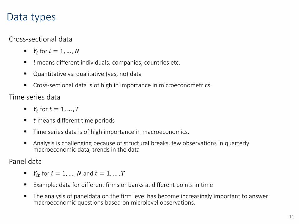
Data types

Cross-sectional data

𝑌𝑖 for 𝑖 = 1,… ,𝑁

𝑖 means different individuals, companies, countries etc.

Quantitative vs. qualitative (yes, no) data

Cross-sectional data is of high in importance in microeconometrics.

Time series data

𝑌𝑡 for 𝑡 = 1,… , 𝑇

𝑡 means different time periods

Time series data is of high importance in macroeconomics.

Analysis is challenging because of structural breaks, few observations in quarterly macroeconomic data, trends in the data

Panel data

𝑌𝑖𝑡 for 𝑖 = 1,… ,𝑁 and 𝑡 = 1, … , 𝑇

Example: data for different firms or banks at different points in time

The analysis of paneldata on the firm level has become increasingly important to answermacroeconomic questions based on microlevel observations.

11

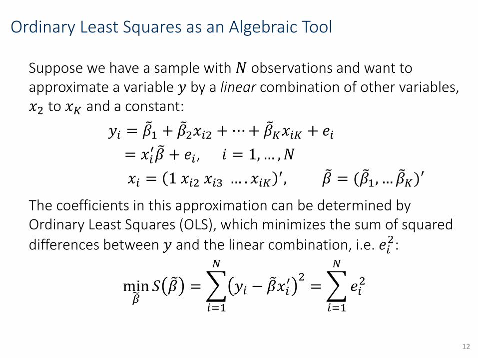
Ordinary Least Squares as an Algebraic Tool

Suppose we have a sample with 𝑁 observations and want to approximate a variable 𝑦 by a linear combination of other variables, 𝑥2 to 𝑥𝐾 and a constant:

𝑦𝑖 = 𝛽1 + 𝛽2𝑥𝑖2 +⋯+ 𝛽𝐾𝑥𝑖𝐾 + 𝑒𝑖

= 𝑥𝑖′ 𝛽 + 𝑒𝑖, 𝑖 = 1,… ,𝑁

𝑥𝑖 = 1 𝑥𝑖2 𝑥𝑖3 … . 𝑥𝑖𝐾′, 𝛽 = ( 𝛽1, … 𝛽𝐾)′

The coefficients in this approximation can be determined by Ordinary Least Squares (OLS), which minimizes the sum of squared

differences between 𝑦 and the linear combination, i.e. 𝑒𝑖2:

min 𝛽

𝑆 𝛽 =

𝑖=1

𝑁

𝑦𝑖 − 𝛽𝑥𝑖′ 2

=

𝑖=1

𝑁

𝑒𝑖2

12

First Order Condition:

This is the Ordinary Least Squares (OLS) estimator. It gives the best linear approximation of 𝑦 from 𝑥2 to 𝑥𝐾 and a constant.

The resulting linear combination of 𝑥𝑖 is given by 𝑦𝑖 = 𝑥𝑖′𝑏 and is the best linear

approximation of 𝑦 from 𝑥2,…,𝑥𝐾 and a constant.

It holds that the error term is orthogonal to the regressors:

So far, pure algebraic derivation with only one assumption that 𝑥𝑖𝑥𝑖′ is

invertible, i.e. none of the 𝑥𝑖𝑘 is an exact linear combination of the other ones and thus redundant.

13

0)~

'(21

ii

N

i

i xyx

i

N

i

i

N

i

ii yxxx

11

' ~

i

N

i

i

N

i

ii yxxxb

1

1

1

'

0)(1

'

1

i

N

i

iii

N

i

i exbxyx

~

)~

(S

Graphical representation for 𝐾 = 2

One can show that , i.e. 𝑏2 is the ratio of the sample covariance between 𝑥 and 𝑦 and the sample variance of 𝑥.

The intercept is determined so as to make the averageapproximation error equal to zero. 14

2

1

12

)(

))((

xx

yyxxb

N

i i

N

i ii

Matrix Notation

In (advanced) econometrics textbooks often matrix notation isused:

The OLS estimator of 𝛽 in Matrix notation is given by:

𝑏 = 𝑋′𝑋 −1𝑋′𝑦

We can decompose 𝑦 as

𝑦 = 𝑋𝑏 + 𝑒

Where it holds that 𝑋′𝑒 = 0 (from the FOC of OLS derivation)

Fitted (or predicted) values: 𝑦 = 𝑋𝑏

15

NN

i

NKN

K

y

y

y

x

x

xx

xx

X

1

'

'

2

112

,

1

1

Ne

e

e 1

By construction, OLS produces the best linear approximation of 𝑦from 𝑥2 to 𝑥𝐾 and a constant. However, without additional assumptions, this approximation has limited value:

The coefficients do not have an economic interpretation

We cannot make statistical statements about these coefficients

The approximation is valid within a given set of observations only

The linear relationship has no general validity outside the current set of values (e.g. in the future or for units not in the sample).

Next, we want to analyse economic relationships that are moregenerally valid than the sample they happen to have.

We want to draw conclusions about what happend if one of the variables actually changes, rather than to describe some historical relation.

Therefore, we introduce a statistical model, the linear regression model.

16

The Linear Regression Model

We now start with a linear relationship between 𝑦 and 𝑥1 ≡ 1 (a constant), 𝑥2 to 𝑥𝐾, which we assume to be generally valid:

The model is a statistical model and is called the population regression model. The error term 𝜀𝑖 contains all influences that are not included explicitly in the model.

The unknown coefficients 𝛽𝑘 have a meaning and measure how we expect 𝑦 to change if 𝑥𝑘 changes (and all other 𝑥 values remain the same, i.e. we apply the ceteris paribus concept).

As a result, OLS produces an estimator for the unknown population parameter vector 𝛽.

17

iiKKii xxy 221

iii xy '

Xy

An estimator is a random variable,

because the sample is randomly drawn from a larger population.

because the data are generated by some random process.

A new sample means a new estimate.

When we consider the different estimates for many different samples, we obtain the sampling distribution of the OLS estimator.

18

The sampling process describes how a sample is taken from thepopulation:

1. 𝑥𝑖 are considered as fixed, i.e. deterministic. A new sample onlyimplies new values for 𝜀𝑖, or equivalently for 𝑦𝑖. Experimental setting, not very relevant for economics, but simplifyingassumption.

2. New sample implies new values for both 𝑥𝑖 and 𝜀𝑖, i.e. each time a new set of 𝑁 observations for (𝑦𝑖 , 𝑥𝑖) is drawn.

Highly relevant in cross-section econometrics

In time series econometrics a random sample of time periods does not make sense. A sample is rather one realization of what could havehappened in a given time span. In a time series context we will need tomake assumption about the way the data are generated (rather thansampled).

19

Important common assumption: 𝐸 𝜀𝑖 𝑥𝑖 = 0 (we say that 𝑥 is exogenous).

It then holds that:

𝐸 𝑦𝑖 𝑥𝑖 = 𝑥𝑖′𝛽

The regression line 𝑥𝑖′𝛽 is an estimate of the conditional expectation of 𝑦𝑖 given the

values for 𝑥𝑖.

We are usually interested in the partial effect of one variable 𝑥𝑘 on 𝐸 𝑦 𝑥1, … , 𝑥𝐾holding all other regressors constant. The partial effect is given by

𝜕 𝐸 𝑦 𝑥1, … , 𝑥𝐾 𝜕𝑥𝑘 = 𝛽𝑘.

Causation vs. Correlation: Simply finding that two variables are correlated is rarely enough to conclude that a change in one variable causes a change in another. There might be a third variable causing correlated changes in the two variables studied.

The notion of ceteris paribus—that is, holding all other (relevant) factors fixed—is at the crux of establishing a causal relationship. What is the (isolated) effect of varying𝑥𝑘 on 𝑦 when holding other influencing factors, i.e. control variables, fixed. Ceteris paribus analysis entails estimating conditional expected values (alternatively we could run controlled experiments, but this is rarely possible in economics, so that we use econometrics instead of lab experiments).

20

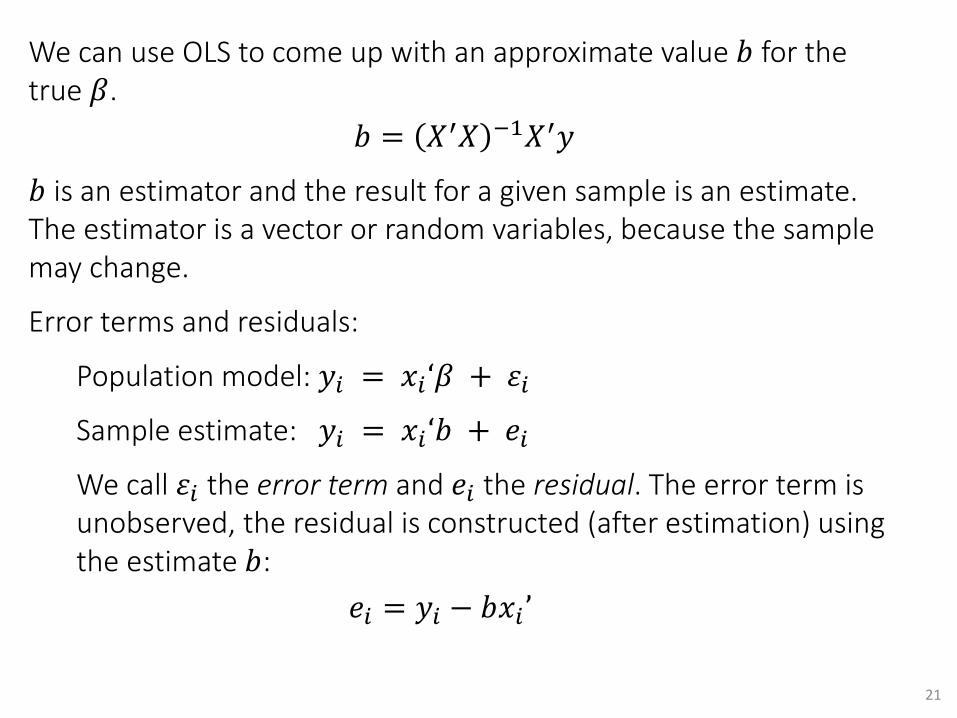
We can use OLS to come up with an approximate value 𝑏 for thetrue 𝛽.

𝑏 = 𝑋′𝑋 −1𝑋′𝑦

𝑏 is an estimator and the result for a given sample is an estimate. The estimator is a vector or random variables, because the sample may change.

Error terms and residuals:

Population model: 𝑦𝑖 = 𝑥𝑖‘𝛽 + 𝜀𝑖

Sample estimate: 𝑦𝑖 = 𝑥𝑖‘𝑏 + 𝑒𝑖

We call 𝜀𝑖 the error term and 𝑒𝑖 the residual. The error term is unobserved, the residual is constructed (after estimation) using the estimate 𝑏:

𝑒𝑖 = 𝑦𝑖 − 𝑏𝑥𝑖 ’

21

Small Sample Properties of the OLS Estimator

Is OLS a good estimator?

The answer to this question depends upon the assumptions we are willing to make.

The most standard and most convenient ones are given by the Gauss-Markov assumptions.

Note that these assumptions are very strong and often not satisfied. Under the Gauss-Markov assumptions, the OLS estimator has nice properties.

Later, we shall discuss how essential the Gauss-Markov assumptions are and how they can be relaxed.

22

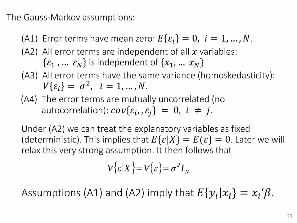
The Gauss-Markov assumptions:

(A1) Error terms have mean zero: 𝐸 𝜀𝑖 = 0, 𝑖 = 1,… ,𝑁.

(A2) All error terms are independent of all 𝑥 variables: {𝜀1 , … 𝜀𝑁} is independent of {𝑥1, … 𝑥𝑁}

(A3) All error terms have the same variance (homoskedasticity): 𝑉 𝜀𝑖 = 𝜎2, 𝑖 = 1,… ,𝑁.

(A4) The error terms are mutually uncorrelated (no autocorrelation): 𝑐𝑜𝑣{𝜀𝑖 , , 𝜀𝑗} = 0, 𝑖 ≠ 𝑗.

Under (A2) we can treat the explanatory variables as fixed (deterministic). This implies that 𝐸{𝜀|𝑋} = 𝐸(𝜀} = 0. Later we will relax this very strong assumption. It then follows that

Assumptions (A1) and (A2) imply that 𝐸 𝑦𝑖 𝑥𝑖} = 𝑥𝑖 ‘𝛽.

23

N

2IσεVXεV

1. Unbiasedness under assumptions (A1) and (A2): 𝐸{𝑏} = 𝛽

Proof: 𝐸 𝑏 = 𝐸 𝑋′𝑋 −1𝑋′𝑦 = 𝐸 𝑋′𝑋 −1𝑋′ 𝑋𝛽 + 𝜀

= 𝐸 𝛽 + 𝑋′𝑋 −1𝑋′𝜀 = 𝛽 + 𝐸 𝑋′𝑋 −1𝑋′𝜀 = 𝛽

Note that unbiasedness holds even if (A3) and (A4) are violated.

2. Under A(1), A(2), A(3) and A(4) the variance of the OLS estimator is given by

𝑉 𝑏 = 𝜎2 𝑋′𝑋 −1

Proof: 𝑉 𝑏 = 𝐸 [𝑏 − 𝛽][𝑏 − 𝛽]′ = 𝐸{ 𝑋′𝑋 −1𝑋′𝑦 − 𝛽 [ 𝑋′𝑋 −1𝑋′𝑦 − 𝛽]′}

= 𝐸 𝑋′𝑋 −1𝑋′ 𝑋𝛽 + 𝜀 − 𝛽 𝑋′𝑋 −1𝑋′ 𝑋𝛽 + 𝜀 − 𝛽 ′

= 𝐸{ 𝛽 + 𝑋′𝑋 −1𝑋′𝜀 − 𝛽 𝛽 + 𝑋′𝑋 −1𝑋′𝜀 − 𝛽 ′}

= 𝐸 𝑋′𝑋 −1𝑋′𝜀𝜀′𝑋 𝑋′𝑋 −1

= 𝑋′𝑋 −1𝑋′(𝜎2𝐼𝑁)𝑋 𝑋′𝑋 −1

= 𝜎2 𝑋′𝑋 −1

3. Gauss-Markov Theorem (based on A(1)-A(4)):

The OLS estimator 𝑏 is BLUE: best linear unbiased estimator for 𝛽, i.e. minimum variance linear unbiased estimator.

24

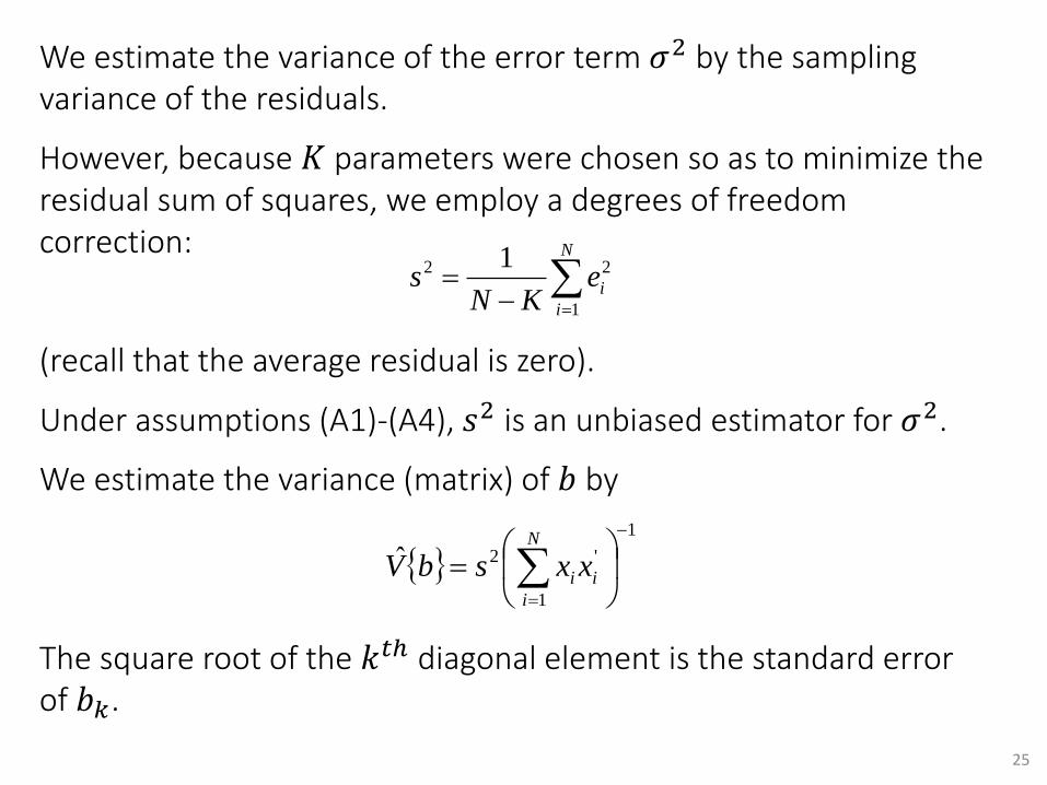
We estimate the variance of the error term 𝜎2 by the sampling variance of the residuals.

However, because 𝐾 parameters were chosen so as to minimize the residual sum of squares, we employ a degrees of freedom correction:

(recall that the average residual is zero).

Under assumptions (A1)-(A4), 𝑠2 is an unbiased estimator for 𝜎2.

We estimate the variance (matrix) of 𝑏 by

The square root of the 𝑘𝑡ℎ diagonal element is the standard error of 𝑏𝑘.

25

N

i

ieKN

s1

22 1

1

1

'2ˆ

N

i

ii xxsbV

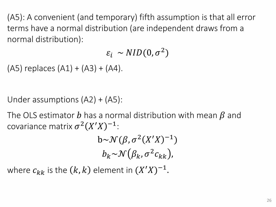
(A5): A convenient (and temporary) fifth assumption is that all error terms have a normal distribution (are independent draws from a normal distribution):

𝜀𝑖 ~ 𝑁𝐼𝐷(0, 𝜎2)

(A5) replaces (A1) + (A3) + (A4).

Under assumptions (A2) + (A5):

The OLS estimator 𝑏 has a normal distribution with mean 𝛽 and covariance matrix 𝜎2 𝑋′𝑋 −1:

b~𝒩(𝛽, 𝜎2 𝑋′𝑋 −1)

𝑏𝑘~𝒩 𝛽𝑘 , 𝜎2𝑐𝑘𝑘 ,

where 𝑐𝑘𝑘 is the 𝑘, 𝑘 element in (𝑋′𝑋)−1.

26

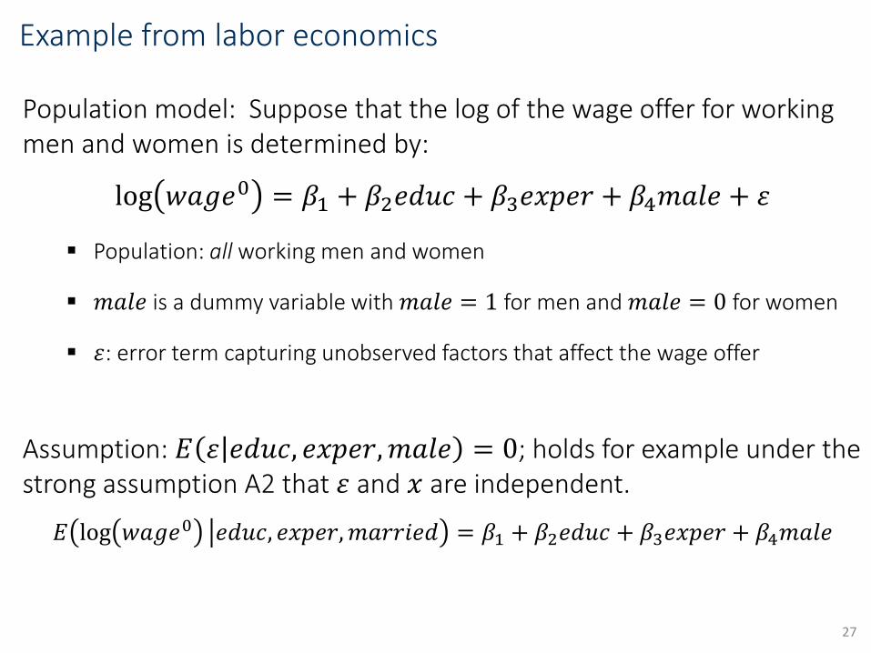
Example from labor economics

Population model: Suppose that the log of the wage offer for workingmen and women is determined by:

log 𝑤𝑎𝑔𝑒0 = 𝛽1 + 𝛽2𝑒𝑑𝑢𝑐 + 𝛽3𝑒𝑥𝑝𝑒𝑟 + 𝛽4𝑚𝑎𝑙𝑒 + 𝜀

Population: all working men and women

𝑚𝑎𝑙𝑒 is a dummy variable with 𝑚𝑎𝑙𝑒 = 1 for men and 𝑚𝑎𝑙𝑒 = 0 for women

𝜀: error term capturing unobserved factors that affect the wage offer

Assumption: 𝐸 𝜀 𝑒𝑑𝑢𝑐, 𝑒𝑥𝑝𝑒𝑟,𝑚𝑎𝑙𝑒 = 0; holds for example under thestrong assumption A2 that 𝜀 and 𝑥 are independent.

𝐸 log 𝑤𝑎𝑔𝑒0 𝑒𝑑𝑢𝑐, 𝑒𝑥𝑝𝑒𝑟,𝑚𝑎𝑟𝑟𝑖𝑒𝑑 = 𝛽1 + 𝛽2𝑒𝑑𝑢𝑐 + 𝛽3𝑒𝑥𝑝𝑒𝑟 + 𝛽4𝑚𝑎𝑙𝑒

27

We are interested in expected changes of the dependent variable when changing a regressor:

By how much dow we expect the wage offer to change, foranother year of schooling, holding fixed all other explanatoryvariables.

Partial effect: 𝜕𝐸 log 𝑤𝑎𝑔𝑒0 𝑒𝑑𝑢𝑐, 𝑒𝑥𝑝𝑒𝑟,𝑚𝑎𝑙𝑒

𝜕𝑒𝑑𝑢𝑐= 𝛽2

Without the assumption 𝐸 𝜀 𝑥 = 0 the error term, i.e. unoberserved factors, have an effect on 𝐸 𝑦 𝑥 so that we cannotestimate partial effects from the observed data.

In this case𝜕𝐸 log 𝑤𝑎𝑔𝑒0 𝑒𝑑𝑢𝑐, 𝑒𝑥𝑝𝑒𝑟,𝑚𝑎𝑙𝑒

𝜕𝑒𝑑𝑢𝑐= 𝛽2 +

𝜕𝜀

𝜕𝑒𝑑𝑢𝑐

28

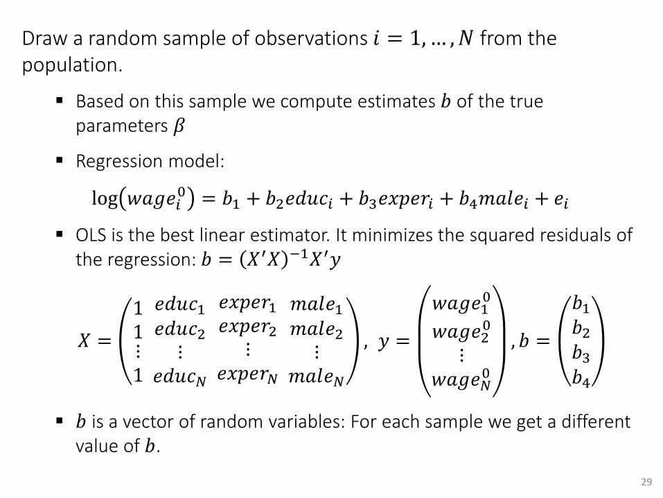
Draw a random sample of observations 𝑖 = 1,… ,𝑁 from thepopulation.

Based on this sample we compute estimates 𝑏 of the trueparameters 𝛽

Regression model:

log 𝑤𝑎𝑔𝑒𝑖0 = 𝑏1 + 𝑏2𝑒𝑑𝑢𝑐𝑖 + 𝑏3𝑒𝑥𝑝𝑒𝑟𝑖 + 𝑏4𝑚𝑎𝑙𝑒𝑖 + 𝑒𝑖

OLS is the best linear estimator. It minimizes the squared residuals ofthe regression: 𝑏 = 𝑋′𝑋 −1𝑋′𝑦

𝑋 =

11⋮1

𝑒𝑑𝑢𝑐1𝑒𝑑𝑢𝑐2⋮

𝑒𝑑𝑢𝑐𝑁

𝑒𝑥𝑝𝑒𝑟1𝑒𝑥𝑝𝑒𝑟2

⋮𝑒𝑥𝑝𝑒𝑟𝑁

𝑚𝑎𝑙𝑒1𝑚𝑎𝑙𝑒2

⋮𝑚𝑎𝑙𝑒𝑁

, 𝑦 =

𝑤𝑎𝑔𝑒10

𝑤𝑎𝑔𝑒20

⋮𝑤𝑎𝑔𝑒𝑁

0

, 𝑏 =

𝑏1𝑏2𝑏3𝑏4

𝑏 is a vector of random variables: For each sample we get a different value of 𝑏.

29

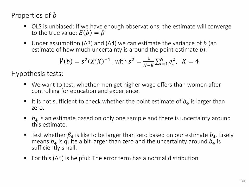
Properties of 𝑏

OLS is unbiased: If we have enough observations, the estimate will convergeto the true value: 𝐸 𝑏 = 𝛽

Under assumption (A3) and (A4) we can estimate the variance of 𝑏 (an estimate of how much uncertainty is around the point estimate 𝑏):

𝑉 𝑏 = 𝑠2 𝑋′𝑋 −1 , with 𝑠2 =1

𝑁−𝐾 𝑖=1𝑁 𝑒𝑖

2, 𝐾 = 4

Hypothesis tests:

We want to test, whether men get higher wage offers than women after controlling for education and experience.

It is not sufficient to check whether the point estimate of 𝑏4 is larger thanzero.

𝑏4 is an estimate based on only one sample and there is uncertainty aroundthis estimate.

Test whether 𝛽4 is like to be larger than zero based on our estimate 𝑏4. Likelymeans 𝑏4 is quite a bit larger than zero and the uncertainty around 𝑏4 issufficiently small.

For this (A5) is helpful: The error term has a normal distribution.

30

Goodness-of-fit

The quality of the linear approximation offered by the model can be measured by the 𝑅2.

The 𝑅2 indicates the proportion of the variance in 𝑦 that can be explained by the linear combination of x variables.

In formula:

Where 𝑦𝑖 = 𝑥𝑖′𝑏 and 𝑦 = (

1

𝑁) 𝑖 𝑦𝑖 denotes the sample mean of 𝑦𝑖.

If the model contains an intercept (as usual), it holds that

31

N

i i

N

i i

i

i

yyN

yyN

yV

yVR

1

2

1

2

2

)()1/(1

)ˆ()1/(1

ˆ

ˆˆ

iii eVyVyV ˆˆˆˆ

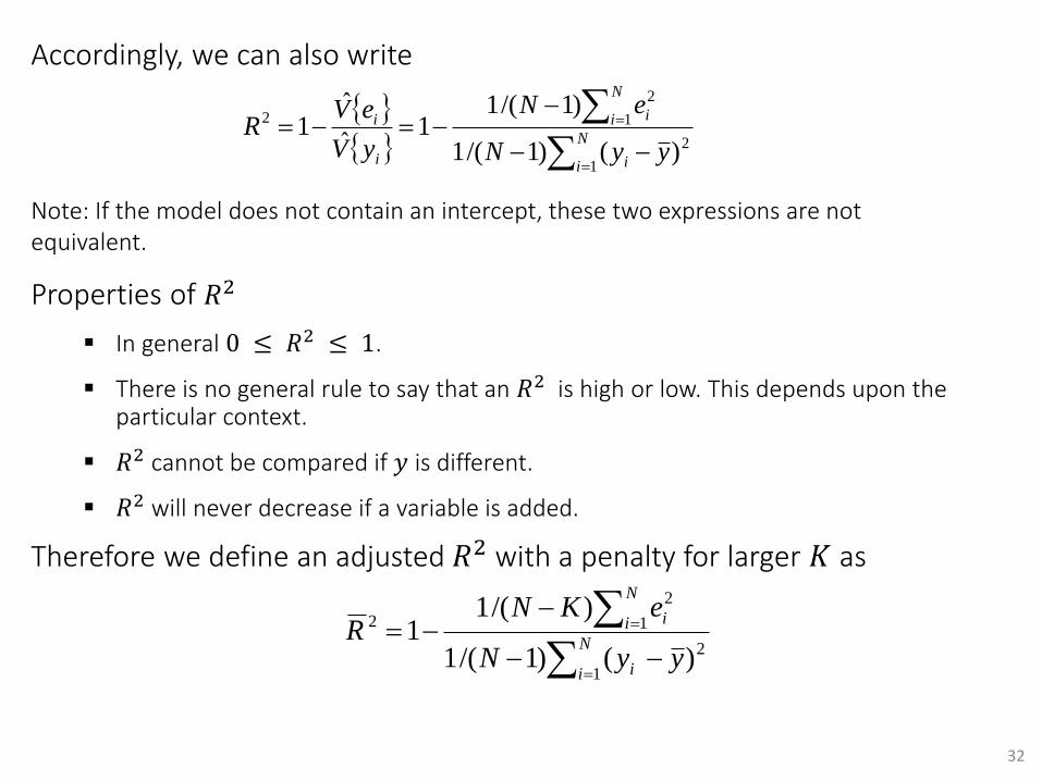
Accordingly, we can also write

Note: If the model does not contain an intercept, these two expressions are not equivalent.

Properties of 𝑅2

In general 0 ≤ 𝑅2 ≤ 1.

There is no general rule to say that an 𝑅2 is high or low. This depends upon the particular context.

𝑅2 cannot be compared if 𝑦 is different.

𝑅2 will never decrease if a variable is added.

Therefore we define an adjusted 𝑅2 with a penalty for larger 𝐾 as

32

N

i i

N

i i

i

i

yyN

eN

yV

eVR

1

2

1

2

2

)()1/(1

)1/(11

ˆ

ˆ1

N

i i

N

i i

yyN

eKNR

1

2

1

2

2

)()1/(1

)/(11

Hypothesis Testing

Often, economic theory implies certain restrictions upon our coefficients. For example, 𝛽𝑘 = 0.

We can check whether our estimates deviate “significantly” from these restrictions by means of a statistical test.

If they do, we will reject the null hypothesis that these restrictions are true.

To perform a test, we need a test statistic. A test statistic is something we can compute from our sample and has a known distribution if the null hypothesis is true.

33

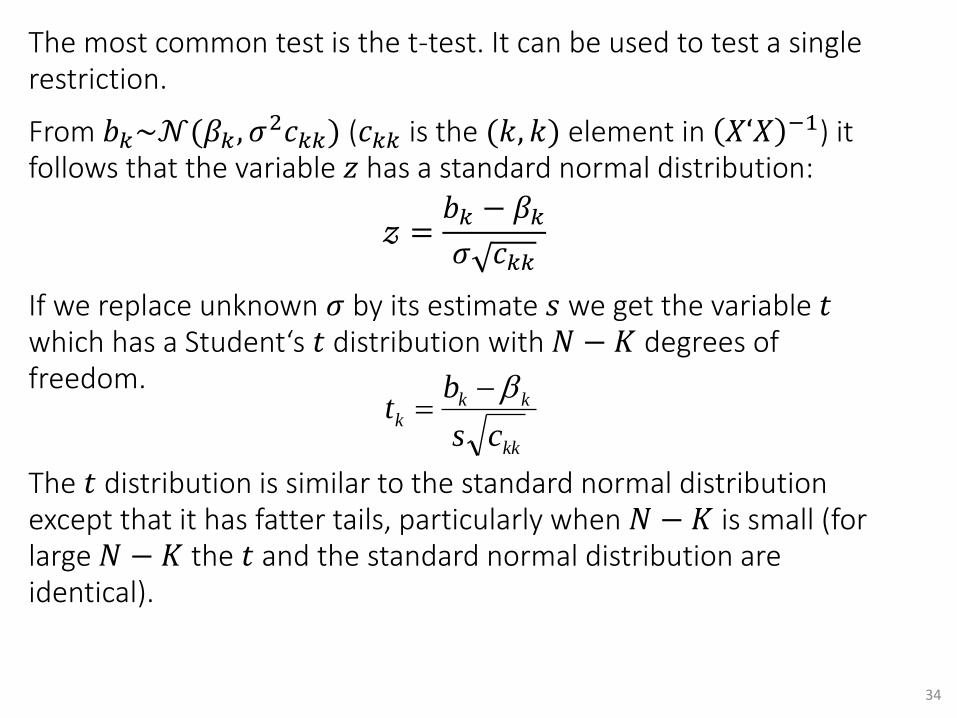
The most common test is the t-test. It can be used to test a single restriction.

From 𝑏𝑘~𝒩(𝛽𝑘 , 𝜎2𝑐𝑘𝑘) (𝑐𝑘𝑘 is the (𝑘, 𝑘) element in 𝑋‘𝑋 −1) it

follows that the variable 𝑧 has a standard normal distribution:

𝓏 =𝑏𝑘 − 𝛽𝑘𝜎 𝑐𝑘𝑘

If we replace unknown 𝜎 by its estimate 𝑠 we get the variable 𝑡which has a Student‘s 𝑡 distribution with 𝑁 − 𝐾 degrees of freedom.

The 𝑡 distribution is similar to the standard normal distributionexcept that it has fatter tails, particularly when 𝑁 − 𝐾 is small (forlarge 𝑁 − 𝐾 the 𝑡 and the standard normal distribution areidentical).

34

kk

kkk

cs

bt

Suppose the null hypothesis is 𝐻0: 𝛽𝑘 = 𝑞 for some given value 𝑞.

Consider the test statistic

𝑡 =𝑏𝑘 − 𝑞

𝑠𝑒(𝑏𝑘).

If the null hypothesis is true, and under the Gauss-Markov assumptions (A1) - (A4) + normality (A5), 𝑡 has a 𝑡-distribution with 𝑁 − 𝐾 degrees of freedom.

We will reject the null hypothesis if the probability of observing a value of |𝑡| or larger is smaller than a given significance level 𝛼, often 5%. From this, one can define the critical values 𝑡𝑁−𝐾;𝛼/2:

Approximating the t-distribution with a standard normal distribution, wereject at the 5% level if

This is a two-sided test, critical values for one-sided test are determinedfrom:

(reject if 𝑡𝑘 > 1.64 based on standard normal approximation)35

2/;KNk ttP

.96.1kt

;KNk ttP

Regression packages typlically report the following 𝑡-value for null hypothesis 𝛽𝑘 = 0:

𝑡𝑘 =𝑏𝑘

𝑠𝑒(𝑏𝑘)

If assumption (A5) does not hold, but the other assumptions (A1)-(A4) hold, the 𝑡-distribution only holds approximately.

The approximation error becomes smaller if the sample size 𝑁becomes larger. We refer to this as asymptotic theory as 𝑁 goes to infinity (𝑁 → ∞).

36

A confidence interval can be defined as the interval of all values for q for which the null hypothesis that 𝛽𝑘 = 𝑞 is not rejected by the t-test.

With probability 1 − 𝛼 the following holds:

Using a standard normal approximation, a 95% confidence interval for𝛽𝑘 is given by:

In repeated sampling, 95% of these interval will contain the true value𝛽𝑘

37

2/;2/;)(

KN

k

kkKN t

bse

bt

)()( 2/;2/; kKNkkkKNk bsetbbsetb

)(96.1),(96.1 kkkk bsebbseb

Suppose we want to test whether 𝐽 coefficients are jointly equal to zero.

The easiest way to obtain a test statistic for this is to estimate the model twice:

once without the restrictions,

once with the restrictions imposed, i.e. with omitting the corresponding 𝑥 variables.

Let the 𝑅2 of the two models be given by 𝑅12 and 𝑅0

2 , respectively. Note that 𝑅1

2 ≥ 𝑅02.

38

The restrictions are unlikely to be valid if the difference between the two 𝑅2 is “large”.

A test statistic can be computed as

Under the null hypothesis (and assumptions (A1)-(A5)), 𝐹 has an 𝐹-distribution with 𝐽 and 𝑁 − 𝐾 degrees of freedom.

We reject if 𝐹 is too large.

For example, with 𝑁 − 𝐾 = 60 and 𝐽 = 3, we reject if

𝐹 > 2.76 (95% confidence).

39

)()1(

)(

2

1

2

0

2

1

KNR

JRR

F

Summary

OLS can be used to approximate a linear combination between different variables, for example to draw a trend line.

For economic applications, we impose additional assumptions, so that weget a statistical model. There is some true population model and OLS canbe used to estimate parameters of the true model.

Under the Gauss-Markov Assumptions OLS has nice properties.

We can interpret a regression model as estimates of conditionalexpectations.

Partial effects have a clear economic interpretation. Based on thestatistical properties of the model we can make statements not onlyabout the given sample, but about the population model, i.e. aboutgeneral economic questions and not only about the specific data that weobserve.

There is uncertainty around the OLS estimates (we just observe one of many samples).

Based on a normality assumption we can construct hypothesis tests(without normality assumption the test are approximately valid).

40