empirical likelihood - mathematicsmai/sta709/owen2005.pdf · fields institute seminar 26 sketch of...

Fields Institute Seminar 1

Empirical Likelihood

Art B. Owen

Department of Statistics

Stanford University

University of Ottawa, May 9 2005


Thanks to

• University of Ottawa

• Fields Institute

• Mayer Alvo

• Jon Rao

This talk

• based on the book “Empirical Likelihood” (2001)∗

• starts with central topics, spirals out, ends with challenges

∗ Chapman & Hall/CRC holds copyright on figures here. They appear with

permission. Book available at www.amazon.com or www.crcpress.com. Book

website at www-stat.stanford.edu/∼owen/empirical



Empirical likelihood provides:• likelihood methods for inference, especially

– tests, and

– confidence regions,

• without assuming a parametric model for data

• competitive power even when parametric model holds



Parametric likelihoodsData have known distribution fθ with unknown parameter θ

Pr(X1 = x1, . . . , Xn = xn) = f(x1, . . . , xn; θ)

Pr(x1 ≤ X1 ≤ x1 + ∆, . . . , xn ≤ Xn ≤ xn + ∆) ∝ f(x1, . . . , xn; θ)

f(· · · ; ·) known, θ ∈ Θ ⊆ Rp unknown

Likelihood function

L(θ) = L(θ; x1, . . . , xn) = f(x1, . . . , xn; θ)

“Chance, under θ, of getting the data we did get”



Likelihood examples

Xi ∼ Poi(θ), θ ≥ 0

L(θ) =n∏

i=1

e−θθxi

xi!

Yi ∼ N(β0 + β1xi, σ2) xi fixed

L(β0, β1, σ) =n∏

i=1

1√2πσ

e−1

2σ2 (yi−β0−β1xi)2



Likelihood inference

Maximum likelihood estimate

θ = arg maxθ

L(θ; x1, . . . , xn)

Likelihood ratio inferences

−2 log(L(θ0)/L(θ)) → χ2(q) Wilks

Typically . . . Neyman-Pearson, Cramer-Rao, . . .

1. θ asymptotically normal

2. θ asymptotically efficient

3. Likelihood ratio tests powerful

4. Likelihood ratio confidence regions small



Other likelihood advantages• can model data distortion: bias, censoring, truncation

• can combine data from different sources

• can factor in prior information

• obey range constraints: MLE of correlation in [−1, 1]

• transformation invariance

• data determined shape for θ | L(θ) ≥ rL(θ)• incorporates nuisance parameters



UnfortunatelyWe might not know a correct f(· · · ; θ)

No reason to expect that new data belong to one of our favorite families

Wrong models sometimes work (e.g. Normal mean via CLT) and sometimes fail

(e.g. Normal variance)

Also,Usually easy to compute L(θ), but . . .

Sometimes hard to find θ

Sometimes hard to compute maxθ2 L((θ1, θ2)) (Profile likelihood)



Nonparametric methodsAssume only Xi ∼ F where

• F is continuous, or,

• F is symmetric, or,

• F has a monotone density, or,

• · · · other believable, but big, family

Nonparametric usually means infinite dimensional parameter

Sometimes lose power (e.g. sign test), sometimes not



Nonparametric maximum likelihood

For Xi IID from F , L(F ) =n∏

i=1

F (xi)

The NPMLE is F =1n

n∑i=1

δxi

where δx is a point mass at x

Kiefer and Wolfowitz, 1956



ProofDistinct values zj appear nj times in sample, j = 1, . . . , m

Let F (zj) = pj ≥ 0 and F (zj) = pj = nj/n with some pj = pj

log(

L(F )

L(F )

)=

m∑j=1

nj log(

pj

pj

)

= n

m∑j=1

pj log(

pj

pj

)

< nm∑

j=1

pj

(pj

pj− 1

)

= 0.



Other NPMLEs

Kaplan-Meier Right censored survival times

Lynden-Bell Left truncated star brightness

Hartley-Rao Sample survey data

Grenander Monotone density for actuarial data



Nonparametric likelihood ratios

Likelihood ratio: R(F ) = L(F )/L(F )

Confidence region: T (F ) | R(F ) ≥ rProfile likelihood: R(θ) = supR(F ) | T (F ) = θConfidence region: θ | R(θ) ≥ r

In parametric setting, −2 log(r) = χ2,1−α(q)



Suppose there are no tiesLet wi = F (xi) wi ≥ 0

∑ni=1 wi ≤ 1

L(F ) =n∏

i=1

wi L(F ) =n∏

i=1

1/n R(F ) =n∏

i=1

nwi

R(θ) = sup n∏

i=1

nwi | T (F ) = θ

If there are ties . . .

L(F ) → L(F ) ×∏j

nnj

j and, L(F ) → L(F ) ×∏j

nnj

j

R and R unchanged



For the meanT (F ) =

∫xdF (x), x ∈ R

d

T (F ) = 1n

∑ni=1 xi

We get T (F ) | R(F ) ≥ ε = Rd, ∀r < 1

Let Fε,x = (1 − ε)F + εδx

For any r < 1,

R(Fε,x) = L((1−ε) bF+εδx)

L( bF )≥ (1 − ε)n ≥ r for small enough ε

Then let δx range over Rd



Fix for the meanRestrict to F (x1, . . . , xn) = 1 i.e.

∑ni=1 wi = 1

Confidence region is

Cr,n = n∑

i=1

wixi | wi ≥ 0,n∑

i=1

wi = 1,n∏

i=1

nwi > r

Profile likelihood

R(µ) = sup n∏

i=1

nwi | wi > 0,n∑

i=1

wi = 1,n∑

i=1

wixi = µ

We have a multinomial on the n data points, hence n − 1 parameters



Multinomial likelihood for n = 3

MLE at center LR= i/10, i = 0, . . . , 9University of Ottawa, May 9 2005


Empirical likelihood theoremSuppose that Xi ∼ F0 are IID in R

d

µ0 =∫

xdF0(x)

V0 =∫

(x − µ0)(x − µ0)T dF0(x) finite

rank(V0) = q > 0

Then as n → ∞−2 logR(µ0) → χ2

(q)

same as parametric limit



Cavendish’s measurements of Earth’s density

4.0 4.5 5.0 5.5 6.0

02

46

Density



Profile empirical likelihood

Density

5.0 5.2 5.4 5.6

0.0

0.2

0.4

0.6

0.8

1.0



Dipper, Cinclus cinclusPossibly copyrighted picture of a dipper bird went here

Eats larvae of Mayflies, Stoneflies, Caddis flies, other



Dipper diet means

Caddis fly larvae

Sto

nefly

larv

ae

0 100 200 300

020

040

060

080

0

Mayfly larvae

Oth

er in

vert

ebra

tes

0 200 600 1000

020

040

060

080

0

Caddis fly larvae

Sto

nefly

larv

ae

0 100 200 300

020

040

060

080

0

Mayfly larvae

Oth

er in

vert

ebra

tes

0 200 600 1000

020

040

060

080

0

IlesUniversity of Ottawa, May 9 2005


Convex Hull

H = H(x1, . . . , xn) = n∑

i=1

wixi | wi ≥ 0,n∑

i=1

wi = 1

µ ∈ H =⇒ logR(µ) = −∞If µ ∈ H we get R(µ) by Lagrange multipliers



Lagrange multipliers

G =n∑

i=1

log(nwi) − nλ′( n∑

i=1

wi(xi − µ))

+ γ( n∑

i=1

wi − 1)

∂

∂wiG =

1wi

− nλ′(xi − µ) + γ = 0

∑i

wi∂

∂wiG = n + γ = 0 =⇒ γ = −n

Solving,

wi =1n

11 + λ′(xi − µ)

Where λ = λ(µ) solves

0 =n∑

i=1

xi − µ

1 + λ′(xi − µ)



Convex duality

L(λ) ≡ −n∑

i=1

log(1 + λ′(xi − µ)) = log R(F )

∂L

∂λ= −

n∑i=1

xi − µ

1 + λ′(xi − µ)

Maximize log R or minimize L

∂2L

∂λ∂λ′ =n∑

i=1

(xi − µ)(xi − µ)′

(1 + λ′(xi − µ))2

L is convex and d dimensional =⇒ easy optimization



Sketch of ELT proof

WLOG q = d, and anticipate a small λ

0 =1n

n∑i=1

xi − µ

1 + (xi − µ)′λ1/(1 + ε) = 1 − ε + ε2 − ε3 · · ·

.=1n

n∑i=1

(xi − µ) − (xi − µ)(xi − µ)′λ, so,

λ.= S−1(x − µ), where,

S =1n

n∑i=1

(xi − µ)(xi − µ)′

Left out: how E(‖X‖2) < ∞ implies small λ(µ0)



Sketch continued

−2 logn∏

i=1

nwi = −2 logn∏

i=1

11 + λ′(xi − µ)

= 2n∑

i=1

log(1 + λ′(xi − µ)) log(1 + ε) = ε − (1/2)ε2 + · · ·

.= 2n∑

i=1

(λ′(xi − µ) − 1

2λ′(xi − µ)(xi − µ)′λ

)

= n(2λ′(x − µ) − λ′Sλ

)= n

(2(x − µ)′S−1(x − µ) − (x − µ)′S−1SS−1(x − µ)

)= n(x − µ)′S−1(x − µ)

→ χ2(d)



Typical coverage errors1. Pr(µ0 ∈ Cr,n) = 1 − α + O

(1n

)as n → ∞

2. One-sided errors of O(

1√n

)cancel

3. Bartlett correction DiCiccio, Hall, Romano

(a) replace χ2,1−α by(1 + a

n

)χ2,1−α for carefully chosen a

(b) get coverage errors O(

1n2

)(c) a does not depend on α

(d) data based a gets same rate

same as for parametric likelihoods



Calibrating empirical likelihoodPlain χ2,1−α undercovers

F 1−αd,n−d is a bit better

Bartlett correction asymptotics slow to take hold

Bootstrap seems to work best



Bootstrap calibration

Recipe

Sample X∗i IID F

Get −2 logR(x; x∗1, . . . , x

∗n)

Repeat B = 1000 times

Use 1 − α sample quantile

Results

Regions get empirical likelihood shape and bootstrap size

Coverage error O(n−2)Same error rate as bootstrapping the bootstrap

Sets in faster than Bartlett correction

Need further adjustments for one-sided inference



Bootstrap (and χ2) calibrated Dipper regions

Caddis fly larvae

Sto

nefly

larv

ae

0 100 200 300

020

040

060

080

0

Mayfly larvae

Oth

er in

vert

ebra

tes

0 200 600 1000

020

040

060

080

0

Caddis fly larvae

Sto

nefly

larv

ae

0 100 200 300

020

040

060

080

0

Mayfly larvae

Oth

er in

vert

ebra

tes

0 200 600 1000

020

040

060

080

0



Resampled −2 logR(µ) values vs χ2

0 5 10 15

05

1015

20

••••••••••••••••••••••••••••••••••••••••••••••••••••••••••••••

•••••••••••••••••••••••••••••••••••••••••••••••••••••••••••••

••••••••••••••••••••••••••••••••••••••••••••••••••••••••••••••••••••••••••••••••••••••••••••••••••••••••••••••••••••••••••••••••••••••••••••••••••••••••••••••••••••••••••••••••••••••••••••••••••••••••••••••••••••••••••••••••••••••••••••••••••••••••••••••••

•••••••••••••••••••••••••••••••••••••••

•••

•

•

0 5 10 15

05

1015

20

•••••••••••••••••••••••••••••••••••••••••••••••••••••••••••••••••••••••••••••••••••••••••••••••••••••••••••••••••••••••••••

••••••••••••••••••••••••••••••••••••••••••••••••••••••••••••••••••••••••••••••••••••••••••••••••••••••••••••••••••••••••••••••••••••••••••••••••••••••••••••••••••••••••••••••••••••••••••••••••••••••••••••••••••••••••••••••••••••••••••••••••••••••••••••••••••••••••••••••••••••••••••••••••••

•••••••••••••••••••••••••••••••

••••

•

0 5 10 15

05

1015

20

•••••••••••••••••••••••••••••••••••••••••••••••••••••••••••••••••••••••••••••••••••••••

•••••••••••••••••••••••••••••••••••••••••••••••••••••••••••••••••••••••••••••••••••••••••••••••••••••••••••••••••••••••••••••••••••••••••••••••••••••••••••••••••••••••••••••••••••••••••••••••••••••••••••••••••••••••••••••••••••••••••••••••••••••••••••••••••••••••••••••••••••••••••••••••••••••••••••••••••••••••••••••••••••••••••••••••••••••••••••••••••••••••••••••••••••••••••••••••••••••••••••••••••••••••••••••••••••••••••••••••••••••••••••••••••••••••••••••••••••••••••••••••••••••••••••••••••••••

Caddis vs Stonefly Mayfly vs other all four



Smooth functions of means

σ =√

E(X2) − E(X)2

ρ =E(XY ) − E(X)E(Y )√

E(X2) − E(X)2√

E(Y 2) − E(Y )2

θ = h(E(U, V, . . . , Z)

Generally

X = (U, V, . . . , Z)

θ = E(h(X))

θ = h(x) .= h(E(X)) + (x − E(X))′∂

∂xh(E(X))

h nearly linear near E(X) =⇒ θ nearly a mean



S&P 500 returns

Trading day

0 50 100 150 200 250

1250

1350

1450

•

••

••

•

•

••

•

•

•

•

•

••••

•••

•

•

•

•

•

•

••

•

•

•

•

•

•

•

•

•

•

••

•

•

••

•

•

•

••

•

•

•

••

••••

•

•••

•

•

•

•

••

•

••

••

•••

•••

• ••

•

••••

••

•

•••• •

•

•

••

•

•

••

••

••

••

•

•

••

•

•

•

•

•

••

•

•

•

•

••

•

•

•

• •

•

•

• ••

•

•

•

•

•

•

••

•

•

•

•

•

•

•

•

•••

•

•

••

• •

••

••

••

•

••

•

••

•

•

•

•

•

••

•

•

••

•

••

•

•

••

•

•

•

•

•

•

•

•

••

••

•

• ••

•

••

•

•

••

•

•

•

••

•

• •

•

••

••

••

••

• •

•

••

•

•

•

•

•••

•••

•••

••

••

•

N(0,1) Quantile

-3 -2 -1 0 1 2 3

-0.0

6-0

.02

0.02

Return = log(xi+1/xi)Nearly N(0, σ2) but heavy tails

Volatility σ is Standard deviation of returns



S&P 500 returns

Annualized Volatility of SP500 (Percent)

18 20 22 24 26 28 30

0.0

0.2

0.4

0.6

0.8

1.0

Solid = Empirical likelihood

Dashed = Normal likelihood



Estimating equationsMore powerful and general than smooth functions

Define θ via E(m(X, θ)) = 0

Define θ via 1n

∑ni=1 m(xi, θ) = 0

Usually dim(m) = dim(θ)

Basic examples: dim(m) = dim(θ) = 1

m(X, θ) Statistic

X − θ Mean

1X∈A − θ Probability of set A

1X≤θ − 12 Median

∂∂x log(f(X ; θ)) MLE under f

−2 logR(θ0) → χ2Rank(V ar(m(X,θ0))) University of Ottawa, May 9 2005


Empirical likelihood for a median

Median pounds of milk

2000 3000 4000 5000

0.0

0.2

0.4

0.6

0.8

1.0

LR is constant between observations



Est. eq. with nuisance parametersFor θ = (ρ) and ν = (µx, µy, σx, σy)E(m(X, θ, ν)) = 0 = 1

n

∑ni=1 m(Xi, θ, ν)

Correlation example

0 = E(X − µx)

0 = E(Y − µy)

0 = E((X − µx)2 − σ2x)

0 = E((Y − µy)2 − σ2y)

0 = E((X − µx)(Y − µy) − ρσxσy)

Profile empirical likelihood R(θ) = supν R(θ, ν)Typically −2 logR(θ0) → χ2

dim(θ)



Huber’s robust estimation

0 =1n

n∑i=1

ψ(xi − µ

σ

)0 =

1n

n∑i=1

[ψ

(xi − µ

σ

)2

− 1]

Like mean for small obs, median for outliers

ψ(z) =

⎧⎨⎩z, |z| ≤ 1.35

1.35 sign(z), |z| ≥ 1.35.

R(µ) = maxσ

max n∏

i=1

nwi | 0 ≤ wi,∑

i

wi = 1,∑

i

wiψ(xi − µ

σ

)= 0,

∑i

wi

[ψ

(xi − µ

σ

)2

− 1]

= 0



Newcomb’s passage times of light

-40 -20 0 20 40

0.0

1.0

2.0

3.0

Passage time

From StiglerUniversity of Ottawa, May 9 2005


EL for mean and Huber’s location

Passage time

-20 0 20 40

0.0

0.2

0.4

0.6

0.8

1.0



Maximum empirical likelihood estimates

Hartley & Rao 1968 means & finite populations

Owen 1991 means IID

Qin & Lawless 1993 estimating eqns IID

Simple MELEs

Observe (Xi, Yi) pairs with mean (µx, µy) and µx = µx0 known

Let wi maximize∏n

i=1 nwi st:

wi ≥ 0 and∑n

i=1 wi = 1 and∑n

i=1 wixi = µx

MELE µy =n∑

i=1

wiyi.= Y − ΣyxΣ−1

xx (X − µx0)



Side or auxiliary information

Known parameter Estimating equation

mean X − µx

α quantile 1X≤Q − α

P (A | B) (1A − ρ)1B

E(X | B) (X − µ)1B



Overdetermined equations

E(m(X, θ)) = 0, dim(m) > dim(θ)

Approaches:

1. Drop dim(m) − dim(θ) equations

2. Replace m(X, θ) by m(X, θ)A(θ) where

A a dim(m) × dim(θ) matrix (IE pick dim(θ) linear comb. of m)

3. GMM: estimate the optimal A

4. MELE: θ = arg maxθ maxwi

∏i nwi st

∑ni=1 wim(xi, θ) = 0

MELE has same asymptotic variance as using optimal A(θ)

Bias scales more favorably with dimensions for MELE than for A methods



Qin and Lawless resultdim(m) = p + q ≥ p = dim(θ) MELE θ

−2 log(R(θ0)/R(θ)) → χ2(p) conf regions for θ0

−2 logR(θ) → χ2(q) goodness of fit tests when q > 0

Requires considerable smoothness

What happens for IQR = Q0.75 − Q0.25 ?

0 = E(1X≤Q.75 − 0.75) = E(1X≤Q.25 − 0.25)

0 = E(1X≤Q.25+IQR − 0.75) = E(1X≤Q.25 − 0.25)

Need to max over Q.25



Euclidean log likelihoodReplace −∑n

i=1 log(nwi) by

E = −12

n∑i=1

(nwi − 1)2

Reduces to Hotelling’s T 2 for the mean Owen

Reduces to Huber-White covariance for regression

Reduces to continuous updating GMM Kitamura

Quadratic approx to EL, like Wald test is to parametric likelihood

Allows wi < 0, and so

1. confidence regions for means can get out of the convex hull

2. confidence regions no longer obey range restrictions



Exponential empirical likelihoodReplace −∑n

i=1 log(nwi) by

KL =n∑

i=1

wi log(nwi)

relates to entropy and exponential tilting

Hellinger distance

n∑i=1

(w1/2i − n−1/2)2



Renyi, Cressie-Read

2λ(λ + 1)

n∑i=1

((nwi)−λ − 1)

λ Method

−2 Euclidean log likelihood

→ −1 Exponential empirical likelihood

−1/2 Freeman-Tukey

→ 0 Empirical likelihood

1 Pearson’s



Alternate artificial likelihoodsAll Renyi Cressie-Read familiies have χ2 calibrations. Baggerly

Only EL is Bartlett correctable Baggerly

−2∑n

i=1 log(nwi) Bartlett correctable if

log(1 + z) = z − 12z2 +

13z3 − 1

4z4 + o(z4), as z → 0

Corcoran



Regression

E(Y | X = x) .= β0 + β1x

Models (Freedman)

Correlation (Xi, Yi) ∼ FXY IID

Regression xi fixed, Yi ∼ FY |X=(1,xi) indep

Correlation model

β = E(X ′X)−1E(X ′Y )

β =( 1

n

n∑i=1

X ′iXi

)−1 1n

n∑i=1

X ′iYi

β and β well defined even for lack of fit



Cancer deaths vs population, by county

Population (1000s)

0.5 5.0 50.0

15

1050

Population (1000s)

0.5 5.0 50.0-5

00

50

Nearly linear regression nonconstant residual variance

Royall via Rice



Estimating equations for regression

E(X ′(Y − X ′β)) = 0,1n

n∑i=1

X ′i(Yi − X ′

iβ) = 0

R(β) = max n∏

i=1

nwi |n∑

i=1

wiZi(β) = 0, wi ≥ 0,n∑

i=1

wi = 1

Zi(β) = X ′i(Yi − X ′

iβ)

need E(‖Z‖2) ≤ E(‖X‖2(Y − X ′β)2

)< ∞

Don’t need:

normality, constant variance, exact linearity



For cancer data

Pi = population of i’th county in 1000s

Ci = cancer deaths of i’th county in 20 years

Ci.= β0 + β1Pi

β1 = 3.58 =⇒ 3.58/20 = 0.18 deaths per thousand per year

β0 = −0.53 near zero, as we’d expect



Regression through the origin

Ci.= β1Pi

Residuals should have mean zero and be orthogonal to P i

We want two equations in one unknown β1

Equivalently, side information β0 = 0

Least squares regression through origin does not solve both equations

MELE β1 = arg maxβ1R(β1)

R(β1) = max n∏

i=1

nwi |n∑

i=1

wi(Ci − Piβ1) = 0,

n∑i=1

wiPi(Ci − Piβ1) = 0,n∑

i=1

wi = 1, wi ≥ 0



Regression parameters

Intercept

-10 -5 0 5

0.0

0.2

0.4

0.6

0.8

1.0

Cancer Rate

3.0 3.2 3.4 3.6 3.8 4.0

0.0

0.2

0.4

0.6

0.8

1.0

Intercept nearly 0, MELE smaller than MLE

CI based on conditional empirical likelihood

Constraint narrows CI for slope by over half



Fixed predictor regression model

E(Yi) = µi.= β0 + β1xi fixed, and V (Yi) = σ2

i

With lack of fit µi = β0 + β1xi

No good definition of ‘true’ β given L.O.F.

Zi = xi(Yi − x′iβ) have

1. mean E(Zi) = xi(µi − x′iβ) 0 may be the common value

2. variance V (Zi) = xix′iσ

2i non-constant, even if σ2

i constant



Triangular array ELT

Z11

Z12 Z22

Z13 Z23 Z33

......

.... . .

Z1n Z2n Z3n · · · Znn

......

.... . .

Row n has indep Z1n, . . . , Znn, common mean 0 not ident distributed

Different rows have different distns

Still get − logR(Common mean = 0) → χ2dim(Z) under mild conditions

Applies for fixed x regression: Zin = xi(Yi − x′iβ)



Variance modellingWorking model Y ∼ N(x′β, e2z′γ)

0 =1n

n∑i=1

xi(yi − x′iβ) e−2z′

iγ (weight ∝ 1/var)

0 =1n

n∑i=1

zi

(1 − exp(−2z′iγ)(yi − x′

iβ)2)

For cancer data

xi = (1, Pi) zi = (1, log(Pi))

E(Yi) = β0 + β1Pi

√V (Yi) = exp(γ0 + γ1 log(Pi)) = eγ0P γ1

i

and β0 = 0



Heteroscedastic model

Cancer Rate

3.2 3.4 3.6 3.8 4.0

0.0

0.2

0.4

0.6

0.8

1.0

Standard Deviation Power

0.5 0.7 0.9

0.0

0.2

0.4

0.6

0.8

1.0

Left: solid curve accounts for nonconstant variance

Right: solid curve forces β0 = 0, and,

rules out γ1 = 1/2 (Poisson) and γ1 = 1 (Gamma)



Nonlinear regression

Time

Ca

upta

ke

0 5 10 15

01

23

45

y.= f(x, θ) ≡ θ1(1 − exp(−θ2x))



Nonlinear regression regions

Theta(1)

The

ta(2

)

3.5 4.0 4.5 5.0 5.5 6.0

0.10

0.20

0.30

0 =n∑

i=1

wi(Yi − f(xi, θ))∂

∂θf(xi, θ)

Don’t need: normality or constant varianceUniversity of Ottawa, May 9 2005


Logistic regression• Giant cell arteritis is a type of vasculitis (inflamation of blood or lymph vessels)

• Not all vasculitis is GCA

• Try to predict GCA from 8 binary predictors

Pr(GCA) .= τ(X ′β) =exp(β0 + β1X1 + · · · + β8X8)

1 + exp(β0 + β1X1 + · · · + β8X8)

Likelihood estimating equations reduce to: Zi(β) = Xi(Yi − τ(X ′β))



Logistic regression coefficients

GCA Intercept

-25 -20 -15 -10 -5

0.0

0.2

0.4

0.6

0.8

1.0

Headache

0 2 4 6 8

0.0

0.2

0.4

0.6

0.8

1.0

Temporal artery

0 2 4 6 8 10 12

0.0

0.2

0.4

0.6

0.8

1.0

Polymyal rheumatism

-2 0 2 4 6

0.0

0.2

0.4

0.6

0.8

1.0

Artery biopsy

2 4 6 8 10 12

0.0

0.2

0.4

0.6

0.8

1.0

Erythrocyte sedimentation rate

-2 0 2 4 6 8

0.0

0.2

0.4

0.6

0.8

1.0

Claudication

0 5 10 15

0.0

0.2

0.4

0.6

0.8

1.0

Age > 50

0 2 4 6 8 10 12 14

0.0

0.2

0.4

0.6

0.8

1.0

Scalp tenderness

-6 -4 -2 0 2 4 6

0.0

0.2

0.4

0.6

0.8

1.0



Prediction accuracy

Smoothed P(Err|Y=0)

0.0 0.04 0.08

0.0

0.2

0.4

0.6

0.8

1.0

Smoothed P(Err|Y=1)

0.0 0.10 0.20 0.30

0.0

0.2

0.4

0.6

0.8

1.0



Biased samplingExamples

1. Sample children, then record family sizes.

2. Draw blue line over cotton, sample fibers that are partly blue.

3. When Y = y it is recorded as X with prob. u(y), lost with prob. 1 − u(y).

Y ∼ F , observe X ∼ G, but we really want F

G(A) =

∫A

u(y) dF (y)∫u(y) dF (y)

L(F ) =n∏

i=1

G(xi) =n∏

i=1

F (xi) u(xi)∫u(x) dF (x)



NPMLE

G(xi) =1n

(for simplicity, suppose no ties)

G(xi) ∝ F (xi) × u(xi)

F (xi) =u−1

i∑nj=1 u−1

j

For the mean

µ =∑n

i=1 xi/ui∑ni=1 1/ui

Horvitz-Thompson estimator is NPMLE

µ =( 1

n

n∑i=1

x−1i

)−1

when ui ∝ xi, so length bias =⇒ harmonic mean



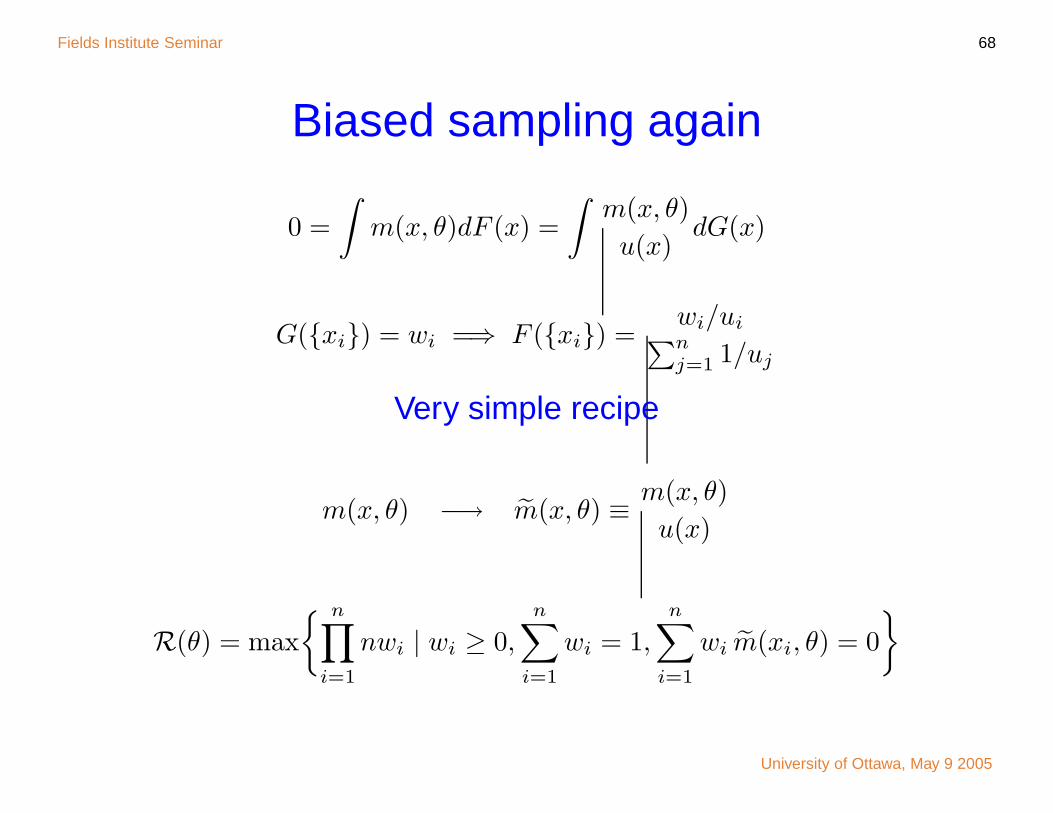
Biased sampling again

0 =∫

m(x, θ)dF (x) =∫

m(x, θ)u(x)

dG(x)

G(xi) = wi =⇒ F (xi) =wi/ui∑nj=1 1/uj

Very simple recipe

m(x, θ) −→ m(x, θ) ≡ m(x, θ)u(x)

R(θ) = max n∏

i=1

nwi | wi ≥ 0,n∑

i=1

wi = 1,n∑

i=1

wi m(xi, θ) = 0



Transect sampling of shrubs (Muttlak & McDonald)

2 4 6 8 10 12

02

46

8

Original Shrub Widths

2 4 6 8 10 12

04

8

Reweighted Shrub Widths



Mean shrub width

0.5 1.0 1.5

0.0

0.2

0.4

0.6

0.8

1.0

0 =n∑

i=1

wixi − µ

xiSolid

0 =n∑

i=1

wi(xi − µ) Dotted



Standard dev. of shrub width

0.2 0.4 0.6 0.8 1.0

0.0

0.2

0.4

0.6

0.8

1.0

0 =n∑

i=1

wi(xi − µ)2 − σ2

xiSolid

0 =n∑

i=1

wi((xi − µ)2 − σ2) Dotted



Multiple biased samplesPopulation k sampled from F with bias uk(·), k = 1, . . . , s

Xik ∼ Gk, i = 1, . . . , nk, k = 1, . . . , s

Gk(A) =

∫A

uk(y) dF (y)∫uk(y) dF (y)

, k = 1, . . . , s

Examples

1. clinical trials with varying enrolment criteria

2. mix of length biased and unbiased samples

3. telescopes with varying detection limits

4. sampling from different frames

NPMLEs Vardi and ELTs Qin by multiplying likelihoodsUniversity of Ottawa, May 9 2005


TruncationExtreme sample bias with

u(x) =

⎧⎨⎩1, x ∈ T

0, x ∈ T

Examples

1. Heights of military recruits, above a mininum

2. Swim times of olympic qualifiers, below a maximum

3. Star too dim to be seen

L(F ) =n∏

i=1

F (xi)∫Ti

dF (x)=

n∏i=1

F (xi)∑j:xj∈Ti

F (xj)



CensoringInstead of exact value, only find that Xi ∈ Ci

Ci = xi incorporates uncensored values

Famous example: right censoring of survival time

Ci =

⎧⎨⎩Xi, Xi ≤ Yi

(Yi,∞), Xi > Yi

Censoring vs truncation

Censoring: Swim times over 3 minutes reported as (3,∞)

Truncation: Swim times over 3 minutes not reported at all



Coarsening at randomFollowing truncation to set Ti,

1. Set Ti partitioned into subsets Ci,ω , ω ∈ Ωi

2. Xi is drawn

3. We only learn which Ci contained Xi

Conditional likelihood for censoring

L(F ) =n∏

i=1

∫Ci

dF (x)∫Ti

dF (x)=

n∏i=1

∑j:xj∈Ci

F (xj)∑j:xj∈Ti

F (xj)conditional on the coarsening



More examplesLeft truncation:

xi = brighness of star

yi = distance

(xi, yi) observed ⇐⇒ xi ≥ h(yi)

Double censoring:

xi = age when child learns to read

yi = age when observation ends, right censoring

zi = age when observation begins, left censoring

Observe xi or [0, zi) or (y,∞]

Left truncation and right censoring:

As above but only non-readers are observed



Some NPMLEsKaplan-Meier for right censored data

F ((−∞, t]) = 1 −∏

j|tj≤t

rj − dj

rj

rj = Number alive at tj−dj = Number dying at tj

Lynden-Bell (conditional likelihood) for left truncated data

F ((−∞, t]) = 1 −n∏

i=1

(1 − 1xi≤t∑n

=1 1y<xi≤x

)

Can have F ((−∞, x(i)] = 1 for some i < n



Some ELTsData type Statistic Reference

Right censoring Survival prob Thomas & Grunkemeier, Li, Murphy

Left truncation Survival prob Li

Left trunc, right cens Mean Murphy & van der Vaart

Right censoring proportional hazard param Murphy & van der Vaart

Right censoring integral vs cum hazard Pan & Zhou



Acute myelogenous leukemia (AML)Embury et al. Weeks until relapse for 11 with maintainance chemotherapy and 12non-maintained

20 week remission probabilities

0.0 0.2 0.4 0.6 0.8 1.0

0.0

0.4

0.8

Increase in 20 week remission probability

-0.5 0.0 0.5 1.0

0.0

0.4

0.8

Increase in median time to relapse

-50 0 50

0.0

0.4

0.8



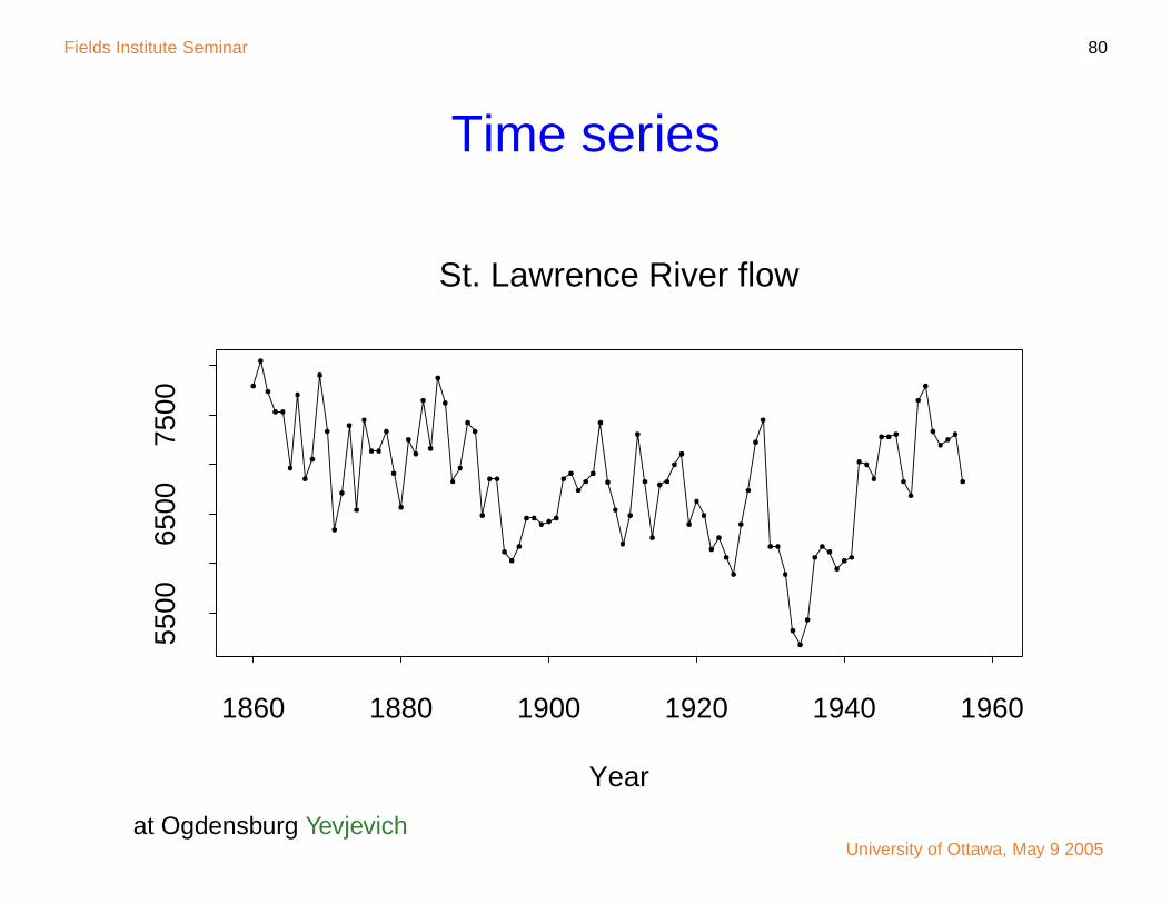
Time series

Year

1860 1880 1900 1920 1940 1960

5500

6500

7500

St. Lawrence River flow

at Ogdensburg YevjevichUniversity of Ottawa, May 9 2005


Reduce to independence

Yi − µ = β1(Yi−1 − µ) + · · · + βk(Yi−k − µ) + εi

E(εi) = 0

E(ε2i ) = exp(2τ)

E(εi(Yi−j − µ)) = 0

j βj −2 logR(βj = 0)

1 0.627 30.16

2 −0.093 0.48

3 0.214 4.05



Blocking of time seriesBlock i of observations, out of n = (T − M)/L + 1 blocks

Bi =(Y(i−1)L+1, . . . , Y(i−1)L+M

)M = length of blocks

L = spacing of start points

Large M = L =⇒ block dependence small

Large M =⇒ block dependence predictable given L

Blocked estimating equation, replace m by b

b(Bi, θ) =1M

M∑j=1

m(X(i−1)L+j, θ)

−2( T

nM

)logR(θ0) → χ2 as M → ∞, MT−1/2 → 0 Kitamura



Bristlecone pinePossibly copyrighted picture of a bristlecone pine went here



5405 years of Bristlecone pine tree ring widths

Campito tree ring data

0 to 100 in 0.01 mm Fritts et al.



Probability of sharp decrease

0.010 0.015 0.020 0.025 0.030 0.035 0.040

0.0

0.2

0.4

0.6

0.8

1.0

Sharp ≡ drop of over 0.2 mm from average of previous 10 years.



MELEs for finite population sampling1. use side information

(a) population means, totals, sizes

(b) stratum means, totals, sizes

2. take unequal sampling probabilities

3. use non-negative observation weights

Hartley & Rao, Chen & Qin, Chen & Sitter

More finite population results

ELTs −2(1 − n

N

)R(µ) → χ2 Zhong & Rao

EL variance ests via pairwise inclusion probabilities Sitter & Wu

Multiple samples varying distortions Zhong, Chen, & Rao



EL hybrids (mostly Jing Qin)Part of the problem parametric

We want to use that knowledge

Rest of the problem non-parametric



One parametric sample, one notY well studied and has parametric distribution

X new and/or does not follow parametric distribution

Xi ∼ F, i = 1, . . . , n

Yj ∼ G(y; θ), j = 1, . . . , m

0 =∫ ∫

h(x, y, φ)dF (x)dG(y; θ)

e.g. φ = E(Y ) − E(X)



Multiply the likelihoods

L(F, θ) =n∏

i=1

F (xi)m∏

j=1

g(yj ; θ)

R(F, θ) = L(F, θ)/L(F , θ)

R(φ) = maxF,θ

R(F, θ) such that

0 =n∑

i=1

wi

∫h(xi, y, φ)dG(y; θ)

Qin gets an ELT



Parametric model for data ranges

X ∼⎧⎨⎩f(x; θ) x ∈ P0

??? x ∈ P0

Examples

• Extreme values with exponential tails on P0 = [T,∞)

• Normal data on P0 = [−T, T ] with outliers

L =n∏

i=1

f(xi; θ)xi∈P0 wxi ∈P0i

Define R using

1 =∫

P0

dF (x; θ) +n∑

i=1

wi1x∈P0

Qin & Wong get an ELT for means



More hybridsParametric Nonparametric

g(y | x; θ) X ∼ F

x ∼ f(x; θ) y | x ∼ Gx Few x vals

x ∼ f(x; θ) (y − µ(x))/σ(x) ∼ G



Bayesian empirical likelihood (Lazar)Prior θ ∼ π(θ)x ∼ F nonparametric

Posterior ∝ π(θ)R(θ)

Here we have informative prior nonparametric likelihood

Reverse of common practice

Posterior regions asymptotically properly calibrated

Justify via least favorable families



Curve estimation problems

fh(x) =1

nhd

n∑i=1

K(xi − x

h

)density

µh(x) =1

nhd

n∑i=1

K(xi − x

h

)Yi regression

Triangular array ELT applies Bias adjustment issues

Dimensions and geometry

Dim(x) Dim(y) Estimate Region

1 ≥ 2 space curve confidence tube

≥ 2 1 (hyper)-surface confidence sandwich



Trajectories of mean blood pressure

Men

Diastolic

Sys

tolic

70 75 80

120

130

140

150

Women

Diastolic

Sys

tolic

70 75 80

120

130

140

150

dots at ages 25, 30, . . . , 80data from Jackson et al., courtesy of Yee



Confidence tube for men’s mean SBP, DBP

30 40 50 60 70 80

Age

120

130

140

150

SBP

6570

7580

85D

BP

Mean blood pressure confidence tube



Empirical likelihood vs bootstrap1. EL gives shape of regions for d > 1

2. EL Bartlett correctable, bootstrap not

3. EL can be faster, but,

4. EL optimization can be hard



Why use anything else?1. Computation is hard

2. Convex hull is binding



Computation

logR(θ) = maxν

logR(θ, ν)

= maxν

minλ

L(θ, ν, λ), where,

L(θ, ν, λ) = −n∑

i=1

log(1 + λ′m(xi, θ, ν)

)

Inner and outer optimizations n dimensional

Used NPSOL, expensive and not public domain (but it works)



Convex hullconfidence regions nested inside convex hull of data

restrictive if d not small

not so bad for one and two dimensional subparameters

possible remedies

1. Empirical likelihood t Baggerley

2. Hybrid with Euclidean likelihood


empirical likelihood - mathematicsmai/sta709/owen2005.pdf · fields institute seminar 26 sketch of...

Documents