emissions analysis of freight transport comparing land-side and

Emissions Analysis of Freight Transport Comparing Land-Side and Water-Side Short-Sea Routes: Development and Demonstration of a Freight Routing and Emissions Analysis Tool (FREAT) FINAL REPORT Prepared for: The United States Department of Transportation Research and Special Programs Administration (Under DTRS56-05-BAA-0001 Full Proposal) Submitted by: James J. Corbett, Ph.D., P.E. University of Delaware James J. Winebrake, Ph.D. Rochester Institute of Technology Jill Hatcher Rochester Institute of Technology Alex E. Farrell, Ph.D. University of California Berkeley

DOT Network Report -- Final

1

Table of Contents

List of Tables ................................................................................................................................. 2 List if Figures................................................................................................................................. 2 1 Summary Information.......................................................................................................... 3

1.1 Contact Information........................................................................................................ 3 1.2 Objective and Summary of Work .................................................................................... 3 1.3 List of Participant Organizations ................................................................................... 3

2 Project Overview................................................................................................................... 4 2.1 Background..................................................................................................................... 4 2.2 Emissions Analysis and Network Optimization .............................................................. 5

3 Methodology ........................................................................................................................ 11 3.1 Overview ....................................................................................................................... 11 3.2 Route Data .................................................................................................................... 12 3.3 Data Relevant to Travel Time ....................................................................................... 15 3.4 Data Relevant to Travel Cost........................................................................................ 18 3.5 Data Relevant to Emissions .......................................................................................... 20 3.6 Freight Data.................................................................................................................. 22

4 The Model: Using Solver .................................................................................................... 22 4.1 Overview ....................................................................................................................... 22 4.2 Elements of the Solver Worksheet................................................................................. 22 4.3 Calculating Travel Time ............................................................................................... 24 4.4 Calculating Travel Cost................................................................................................ 26 4.5 Calculating Pollutant Emissions................................................................................... 27 4.6 Formulae in Optimization Columns.............................................................................. 27 4.7 Defining the Constraints in a Network Flow Model..................................................... 27 4.8 Solver Results................................................................................................................ 30

5 Model Demonstration and Modified Cases ...................................................................... 30 5.1 Comparison of the Top Three Optimal Solutions for Each Objective .......................... 30 5.2 Modified Case Study A: Imposing Drayage Cost Penalties on Same-Mode Route Connections............................................................................................................................... 32 5.3 Modified Case Study B: Seeking Alternate, Less Congested Routes ............................ 32

6 Discussion of the Model’s Capabilities and Limitations ................................................. 36 6.1 Capabilities ................................................................................................................... 36 6.2 Limitations .................................................................................................................... 36

7 Conclusion ........................................................................................................................... 37 8 References............................................................................................................................ 40 9 Appendix: Full list of route segments for project case study.......................................... 43


2

List of Tables Table 1. Description of the Model Inputs and Outputs................................................................................. 9 Table 2. Node Reference List .................................................................................................................... 12 Table 3. Selected Part of Master Route List and Distances ....................................................................... 13 Table 4. State- and Port-Specific Speed Limits (mph) .............................................................................. 15 Table 5. Percentage of Maximum Speed Limits........................................................................................ 16 Table 6. Drayage Time .............................................................................................................................. 16 Table 7. Defining the Congestion Index for Each Node............................................................................ 17 Table 8. Defining the Congestion Index for Each Route Segment ............................................................ 18 Table 9. Rate-per-Mile ($/mile) ................................................................................................................. 18 Table 10. Drayage Cost.............................................................................................................................. 19 Table 11. Emission Factors and other Designates ..................................................................................... 21 Table 12. Summary of Emission Factors (g/TEU-mi) ............................................................................... 21 Table 13. Quantity of TEU Containers ...................................................................................................... 22 Table 14. Components of the Solver Worksheet and their Functions........................................................ 23 Table 15. Network Flow Constraints ......................................................................................................... 28 Table 16. Mathematical Representation of Net Flow Constraints ............................................................. 28 Table 17. Example Trip Layout ................................................................................................................. 28 Table 18. Example Optimization Results .................................................................................................. 30 Table 19. The Original Cost Optimal Solution .......................................................................................... 34 Table 20. The Original Cost Optimal Solution: Route Selection............................................................... 34 Table 21. Drayage Cost Altered Case: The New Optimal Solution........................................................... 34 Table 22. Drayage Cost Altered Case: Route Selection ............................................................................ 34 Table 23. Congestion Index (CI) Selections for Case Study 2 .................................................................. 35 Table 24. Optimization Results for Case Study 2 ...................................................................................... 35 Table 25. Resulting Trip Layout for Case Study 2 .................................................................................... 36 List if Figures Figure 1. a) Modal share in 1997; and b) change since 1980 in domestic ton-miles carried by

mode........................................................................................................................................ 4 Figure 2. Emissions from U.S. freight transportation..................................................................... 6 Figure 3. Emissions trends from multimodal freight modes as a percent of total mobile source

emissions a) combined truck, marine, and rail; b) for heavy-duty diesel trucks; and c) for marine vessels. ........................................................................................................................ 7

Figure 4. Schematic of the FREAT Model ..................................................................................... 8 Figure 5. Freight Network Nodes and Routes from “A” to “B” (Solid – onroad trucking, dashed –

rail)........................................................................................................................................ 10 Figure 6. Exploring Tradeoffs for Different Objectives ............................................................... 11 Figure 7. Example Solver Parameters Dialog Box ...................................................................... 29 Figure 8. Comparison of the 2nd and 3rd Optimal Solutions to the Optimal within Each Measured

Output ................................................................................................................................... 31 Figure 9. Comparison of 1st, 2nd and 3rd Optimal Solutions to Single-constraint Solutions across

Other Measures ..................................................................................................................... 33 Figure 10. Constraints Used in Case Study 2 .............................................................................. 35 Figure 11. Time and CO2 Tradeoffs Among Optimal Solutions ................................................. 38 Figure 12. Mode share comparison for various solutions according to distance traveled and CO2

emissions............................................................................................................................... 39


3

Emissions Analysis of Freight Transport Comparing Land-Side and Water-Side Short-Sea Routes: a Freight Routing and Emissions Analysis Tool

(FREAT)

(DRAFT) FINAL REPORT 1 Summary Information

1.1 Contact Information University of Delaware Point of Contact: Dr. James J. Corbett Mailing Address:

Graduate College of Marine Studies 305 Robinson Hall University of Delaware Newark, DE 19716

Telephone Number: 302-831-0768 Fax Number: 302-831-6838 Email Address: [email protected]

Rochester Institute of Technology Dr. James J. Winebrake Mailing Address:

STS/Public Policy Department 92 Lomb Memorial Dr. Rochester Institute of Technology Rochester, NY 14623

Telephone Number: 585-475-4648 Fax Number: 585-475-2510 Email Address: [email protected]

1.2 Objective and Summary of Work This study develops the Freight Routing and Emissions Analysis Tool (FREAT), a

spreadsheet-based decision tool that can assist in evaluating the economic, environmental, and congestion issues associated with alternative land-side and water-side freight transport routes. FREAT develops the methodology and tools for: (1) quantifying emissions from multimodal land-side and water-side freight transport alternatives; (2) evaluating tradeoffs among pollutant emissions, costs, and travel time for moving freight between two points; and, (3) identifying preferred modal combinations within a network of travel paths that would lead to either minimum emissions, minimum costs, or minimum travel time. The decision tool applies an optimization solver to compare routes for various decision objectives (e.g., minimize emissions, minimize costs, or minimize time) and constraints. For emissions, total fuel cycle emissions of GHGs and other pollutants are included. We demonstrate the FREAT model through a case study comparing freight modes along the I-95 corridor. This work supports national and international efforts to understand the value and implications of multimodal freight transportation within an integrated analytic framework. Results identify potential to improve freight service and environmental stewardship in multimodal transportation through a rebalance of modal shares in some cargoes and routes.

1.3 List of Participant Organizations James J. Corbett, Ph.D. (Lead) University of Delaware Center for Marine Policy Studies Ph: (302) 831-0768 E: [email protected]

James J. Winebrake, Ph.D. Rochester Institute of Technology STS/Public Policy Department Ph: (540) 475-4648 E: [email protected]

Alex E. Farrell, Ph.D. University of California, Berkeley Energy Resources Group Ph: (510) 882-6984 E: [email protected]


4

2 Project Overview

2.1 Background Demand for freight transportation is increasing, but not equally across all modes.

According to the Freight Analysis Framework [Federal Highway Administration and Lambert, 2002],1 domestic freight volumes will grow by more than 65 percent from 1998 levels by the year 2020, increasing from 13.5 billion tons (in 1998) to 22.5 billion tons (in 2020). International freight is forecast to grow even faster than domestic trade. However, since 1980 truck freight has doubled (an average annual increase of 3.7%) while domestic waterborne freight has declined by nearly 30% (an average annual decline of 1.8%) [Bureau of Transportation Statistics, 2004].2 Figure 1 illustrates these changes. This translates into significant emissions of greenhouse gases (and other pollutant emissions) for the transportation sector. Trucking alone accounts for nearly 20% of the total CO2 from transportation; domestic waterborne freight movements accounts for less than 5% [Davis, 2003].

a)

0

10

20

30

40

50

60

70

Value Tons Ton-miles

Perc

ent

Truck (private and for-hire) Parcel, postal and courierWater Air (including truck and air)Rail (includes truck and rail) PipelineOther and unknown

b)

0

50

100

150

200

250

1980 1985 1990 1995 2000

Inde

x: 1

980=

100

Intercity truckClass I railWater Oil pipeline

Figure 1. a) Modal share in 1997; and b) change since 1980 in domestic ton-miles carried by mode.

1 See Freight Analysis Framework documents at http://ops.fhwa.dot.gov/freight/freight_analysis/faf/. 2 BTS Pocket Guide to Transportation 2003, http://www.bts.gov/publications/pocket_guide_to_transportation/2003/.


5

The publicly available GeoFreight tool projects that regional growth in truck freight traffic

(and possibly congestion) will be significantly greater than forecasted growth in waterborne freight [Department of Transportation et al., 2003].3 For example, along the East Coast (I-95 Corridor) from Maine to Florida, GeoFreight forecasts for 2010 suggest that modal intensity of highway trucking along I-95 is more than 100 times greater than domestic shipping along the same route (with an intensity index of 0.01 for shipping compared to an intensity index of 1.12 for trucking).4 The I-95 highway corridor also has some of the most congested roads in the nation, which translates into wasted fuel, and increased environmental impacts, such as road dust and oil and more greenhouse gas and criteria pollutant emissions as trucks moving freight are stuck in traffic.

It has been widely acknowledged in the U.S. and in Europe that adjusting the modal share of freight transport can significantly address regional mobility, congestion, and environmental problems [Donnelly and Mazières, 1999; European Commission, 1999; Intergovernmental Panel on Climate Change et al., 2007; Maritime Administration, 2003; 2004; Yonge, 2004].5 Climate change comparisons among modes have also been made [Skjølsvik et al., 2000], but less clearly quantified for U.S. intermodal freight transportation. Current efforts by the U.S. Department of Transportation to investigate and promote short-sea shipping alternatives would benefit from additional focused study comparing the emissions of greenhouse gases and other pollutants among freight modes.

2.2 Emissions Analysis and Network Optimization

2.2.1 Problem Statement Emissions associated with transporting freight can be significant [Energy Information

Administration, 1998; Organisation for Economic Co-Operation and Development (OECD) and Hecht, 1997; Skjølsvik et al., 2000]; in fact, U.S. EPA data suggests that heavy duty truck, rail, and water transport together account for more than 20% of CO2 emissions, about 50% of recent NOx emissions and nearly 40% of the PM emissions from all mobile sources [Environmental Protection Agency, 2005a; Environmental Protection Agency, 2005b]. The distribution of NOx and PM10 emissions in freight transportation is shown in Figure 2 [Cambridge Systematics Inc., 2005]. The largest portion of national emissions from freight comes from heavy-duty vehicles, which produce two-thirds of NOx and PM-106 emissions. Emissions from marine vessels account for 18% of freight NOx emissions and 24% of freight PM-10 emissions, followed by railroads at 15% NOx and 12% PM10.

With demand for freight services increasing, emissions from freight transportation are expected to increase. Air quality impacts from this growing transportation sector need to be studied and effectively modeled for planning purposes. One notable model is the EPA’s Freight Logistics Environmental and Energy Tracking (FLEET) Performance Model, part of the SmartWay Transport Partnership. Through the Partnership, freight carriers can use the FLEET 3 See Geofreight information at http://www.fhwa.dot.gov/freightplanning/geofreight.htm 4 Geofreight’s “use intensity index” is a relative number useful for comparisons. Indices less than 1 signify low intensity. Indices above 2 signify high intensity. This may not reflect local intensity at bottlenecks at ports and other intermodal facilities. 5 Also see U.S. DOT Maritime Administration, http://www.marad.dot.gov/Programs/shortseashipping.html. 6 Particulate matter with a diameter of 10 microns or less.


6

Performance Model to assess either a trucking or rail carrier’s environmental performance with respect to CO2, NOx, or PM emissions. The FLEET Performance Model also allows evaluation of the payoffs of using emissions reduction strategies and fuel savings, demonstrating the financial and environmental benefits of reducing their emissions [U.S. Environmental Protection Agency, 2007].

0%

10%

20%

30%

40%

50%

60%

70%

80%

90%

100%

NOx PM-10 GHGs

Heavy-Duty Trucks Freight Railroad Marine Freight Air Freight

Figure 2. Emissions from U.S. freight transportation.

Figure 3 shows that recent trends suggest little change in modal contribution to CO2; longer-term trends show increased NOx emissions until about 2002 (mostly from heavy duty trucks 2002), but significant PM2.5 reductions (mostly a result of heavy-duty trucking emission reductions). As emissions from these alternatives become more important in local pollution and GHG inventories, decision makers will need tools to compare alternative shipping modes, both separately and in combinations serving logistics supply chains. Unfortunately, insufficient research exists directly comparing alternative land-side and water-side shipping options. The PIs comparisons of land-side and water-side commuting alternatives in California and New York [Farrell et al., 2002b] are among the recently emerging peer-reviewed tools that rigorously analyze the land-side v. water-side modal mix. This work develops the tools needed for the step from passenger transportation comparisons to multimodal freight comparisons that will significantly contribute to the policy analysis and research in this area.


7

0%

10%

20%

30%

40%

50%

60%

1965 1970 1975 1980 1985 1990 1995 2000 2005

Perc

etn

of e

mis

sion

s fr

om a

ll m

obile

sou

rces

NOx Combined HD Truck, Marine, Rail NOx Heavy-Duty Diesel VehiclesNOx Marine Vessels PM2.5 Combined HD Truck, Marine, RailPM2.5 Heavy-Duty Diesel Vehicles PM2.5 Marine VesselsCO2 Combined HD Truck, Marine, Rail CO2 Heavy-Duty Diesel Vehicles

Figure 3. Emissions trends from multimodal freight modes as a percent of total mobile source emissions a) combined truck, marine, and rail; b) for heavy-duty diesel trucks; and c) for marine vessels [Environmental Protection Agency, 2005a; Environmental Protection Agency, 2005b].

In addition, the project scope defined several criteria that should be addressed in the

development of a decision tool that can analyze water-side v. land-side alternatives. We call this tool the Freight Routing and Emissions Analysis Tool (FREAT). These criteria are:

(1) The tool should be user-friendly and available to a wide-audience. We have built

the tool in MS Excel.

(2) The tool should include total fuel cycle emissions. Total fuel-cycle analysis involves consideration of energy use and emissions from the extraction of feedstock (e.g., oil from the well) to the processing of that feedstock into fuel products, to the ultimate use of the fuel in operation. Although recognized as an important analytical approach, EPA (through its MOVES work) has only recently begun to incorporate TFC analyses for light-duty vehicles into its modeling regimen.7 A new model (TEAMS), partly funded by DOT Center for Climate Change and Environmental Forecasting, is also available that conducts total fuel cycle analyses for marine vessels (see http://climate.volpe.dot.gov/areas.html) [Winebrake et al., 2007].

(3) The tool should help evaluate a rich array and diversity of decision questions. In

particular, the tool should include not only parametric analysis, but also optimization routines that allow decision makers to evaluate optimal decisions under various objectives and constraints.

7 The total fuel cycle analysis approach promoted by EPA is reflected in Argonne National Lab’s GREET model for light-duty vehicles.


8

(4) The model can be used to aid in group and multi-lateral decision making by incorporating the objective functions, constraints, and data preferred by different interested parties. By being built on a transparent, well-known platform, the FREAT model can facilitate better analysis and decision-making.

This study creates a decision tool that can assist in evaluating the economic, environmental, and congestion issues associated with alternative land-side and water-side freight transport routes.

FREAT is a spreadsheet-based decision tool that meets these criteria. A final outcome of

our work is the enclosed Excel model (discussed below) that uses optimization routines to assist decision makers in evaluating the environmental, economic, energy use, and temporal, and other tradeoffs associated with intermodal freight transportation.

2.2.2 Research Approach The overall modeling approach we used is demonstrated in Figure 4 and Table 1. We

developed a spreadsheet based model that will accept freight and route data, characteristics of land-side and water-side short-sea shipping alternatives, and environmental data. This information is processed and sent through an optimization algorithm. Users are able to modify default assumptions.

LandsideOperation

Data

LandsideEmissions

Data

Output

OptimizationModel

Freight/RouteData

WatersideOperation

Data

WatersideEmissions

Data

LandsideOperation

Data

LandsideEmissions

Data

Output

OptimizationModel

Freight/RouteData

WatersideOperation

Data

WatersideEmissions

Data

Figure 4. Schematic of the FREAT Model

We develop a common intermodal model using default assumptions representative of current fleets, although the tool allows users to specify modal inputs for activity, power, and emissions. We have used a similar approach without the additional benefits of optimization techniques and a total fuel cycle context for intermodal analyses of freight [Skjølsvik et al., 2000]. This flexible approach allows users to update inputs to the tool with their own information or to use insights from other mobile source models such as the federal EPA MOVES model, or California’s EMFAC2002 model, both of which we have used in previous multimodal studies [Farrell et al., 2002a; Farrell et al., 2003; WestStart-CALSTART et al., 2001; Winebrake et al., 2005]. We have also incorporated best estimates of data related to intermodal freight


9

movement [Environmental Protection Agency, 1997; Sawyer et al., 2000; Yanowitz et al., 1999; Yanowitz et al., 2000], and with related modeling efforts in Europe, such as the Swedish Network for Transportation and the Environment (Nätverket för Transporter och Miljön, or NTM).8

Table 1. Description of the FREAT Model Inputs and Outputs

Freight/Route Data – involves data related to the type of freight, volume/weight considerations, and other characteristics of freight that help dictate the types of land-side or water-side technologies that can be used, as well as the route characteristics and requirements needed to move such freight.

Land-side Factors (Operations and Emissions) – involves data and analysis related to the movement of the freight on land, including mode, fuel type, emissions control technologies, and emissions factors (based on end-use and total fuel cycle emissions).

Water-side Factors (Operations and Emissions) – involves data and analysis related to the movement of the freight on water, particularly short-sea routes. This includes vessel type, fuel type, route characteristics, emissions control technologies, and emissions factors (based on end-use and total fuel cycle emissions)

Land-Side and Water-Side Optimization Model and Output – provides an optimization module that allows decision makers to identify optimal routes, modes, and technologies in order to move freight between two points. The optimization module will allow users to optimize modes/routes based on minimizing costs, minimizing emissions, or minimizing travel time. The results allow for comparative analysis of land-side v. water-side movement of freight under various assumptions, constraints, and optimization objectives.

The optimization aspect of the model is important, and for that reason we discuss it in

detail here. Through the optimization routine, we allow decision makers to consider water-side and land-side shipping alternatives under various objectives and constraints. This research builds on previous work related to travel optimization [Xu et al., 2003a; Xu et al., 2003b]; however, our model includes explicit environmental objectives that address greenhouse gas and pollutant reduction goals. We model discrete freight volumes that may be transported by different multimodal combinations within an optimization framework that considers emissions, technologies, and costs. This extends optimization modeling for environmental and transportation goals, building on team expertise developed over several multimodal analyses [Corbett and Chapman, 2003; Farrell et al., 2003; Farrell et al., 2005; Skjølsvik et al., 2000; Winebrake et al., 2005].

2.2.3 Illustration of Modeling Context Our model can be illustrated through a simple example. Figure 5 shows a network of

alternative pathways to move freight from point A to point B. Freight can move along pathways through each node (shown by the circles). Certain routes (represented by lines connecting the nodes) may be accessible only by truck, or ship, or rail. Some routes may be accessible by multiple modes. Nodes can be associated with metropolitan traffic characteristics, descriptive of

8 See http://www.ntm.a.se/.


10

congestion delays, engine load and emissions patterns that may differ from open freeway, long-haul rail, and/or interport segments.

A BA B

Figure 5. Freight Network Nodes and Routes from “A” to “B” (Solid – onroad trucking, dashed – rail)

The decision maker may wish to analyze alternative pathways from A to B under various

assumptions, constraints, and objectives. For example, one may want to know what pathway leads to the least cost transport of freight from A to B, a traditional context for the application of optimization routines. To analyze this, each route from node i to node j must include a dataset that helps characterize that route. That dataset would include information about mode accessibility, costs, average speed, distance, emissions, among others. For a least cost example, we can set up a network optimization model of the form:

∑ ⋅ijk

ijkijk XCmin

where Cijk is the cost of moving freight from node i to node j using mode k; and Xij is a binary variable that takes on a value of “1” if mode k is used to move freight from i to j, and “0” otherwise. (We have simplified this example for this report; cost components are calculated in the model based on variable, fixed, and other components that affect cost). This model is controlled through constraints (not included here for brevity) that ensure that freight leaves A and gets to B. Other constraints (for example, not allowing water modes to operate between land-bound nodes) are allowed in the model design.

In this work, we model this network system with other optimization objectives. For example, the user may want to explore the pathway (again, characterized by routes and modes) that minimizes emissions of greenhouse gases (or other pollutants). The user then would use a model with the following objective:

∑ ⋅ijk

ijkijk XEmin


11

where Eijk is the emissions associated with moving freight from node i to node j using mode k. (Again, for simplicity we don’t show all the equations associated with calculating the emissions; but they are calculated within the model based on emissions factors and other variables).

Other objectives that FREAT will allow are energy consumption and travel time. The model allows users choice among traditional objectives of cost and time or environmental and energy objectives. This aspect of our research extends significantly beyond prior multimodal analyses and case studies that are primarily descriptive [Corbett and Fischbeck, in preparation 2005; Organisation for Economic Co-Operation and Development (OECD) and Hecht, 1997; Schipper and Marie-Lilliu, 1999; Schipper et al., 1997; Skjølsvik et al., 2000].

One could use the model for numerous types of decision analysis. For example, the user could simply identify optimal routes to meet a particular objective under varying constraints and assumptions. Users could also use it to explore tradeoff curves, an example of which is shown in Figure 6. This curve demonstrates the tradeoff between costs and GHG emissions. Along the curve are representative “optimal solutions”; these solutions correspond to a particular pathway (routes, mode, technologies) for moving freight from A to B. Finally, users can explore the impact of alternative technologies on identical routes—e.g., one could run one route analysis using diesel fuel and then run the identical route using biodiesel to compare emissions impacts. We demonstrate the model and its many uses through a case study discussed in the next section.

Greenhouse Gas Emissions

Cos

t

Four different solutions for exploring the tradeoff between Cost and GHG Emissions.

Greenhouse Gas Emissions

Cos

t

Four different solutions for exploring the tradeoff between Cost and GHG Emissions.

Figure 6. Exploring Tradeoffs for Different Objectives

3 Methodology

3.1 Overview The FREAT model, designed with a Microsoft Excel interface, is equipped to perform

nonlinear optimization of travel time, travel cost, VOC, CO, NOx, PM, SOx, and CO2 emissions. The foundation of the model is the selection of a set of nodes and route segments that, in the optimization process, combine to create the most optimal trip layout. The characterization and definition of these nodes and route segments is a core element of the model.

The model is outfitted with two main worksheets: the Inputs worksheet, and the Solver worksheet. The Inputs worksheet is the source of all interchangeable data used in the optimization process, which takes place on the Solver worksheet. On the Solver worksheet,


12

optimization of travel time, travel cost, and emissions of VOC, CO, NOx, PM, SOx, and CO2 take place. The following section describes the components of the Inputs worksheet, the source of the data therein, and the functions in the Solver worksheet. Regarding the Tables that are from the Inputs sheet and are listed in the following sections, take note that cells shaded in gray are cells that the model user can alter at any time. Cells that are not colored are automatic, and should not be altered.

3.2 Route Data

3.2.1 Route Structure The first data category on the Inputs worksheet is Route Data. Transportation

infrastructure representation is perhaps the most important element of the model. This is because the selection of freight nodes and routes segments, as well as their distances, is a major factor in minimizing the time, cost, and emissions of transporting freight from an origin to a destination. This section contains data relevant to the master route list and node definitions.

Table 2 displays the master node references, each attributed by an identifier number as well as the city name and its abbreviation. These nodes, arranged in a combination of origins and destination nodes, are the building blocks of the route segments. For demonstration purposes and to meet project scope, we present the model using 11 nodes on the East Coast.

Table 2. Node Reference List

City Abbrev. City Name State Node #

NYC New York NY 1

PHL Philadelphia PA 2

WLM.DE Wilmington DE 3

BLT Baltimore MD 4

RCH Richmond VA 5

NFK Norfolk VA 6

WLM.NC Wilmington NC 7

FLO Florence SC 8

CHL Charleston SC 9

SAV Savannah GA 10

JAX Jacksonville NC 11

Shown as Section 1.1 on the Inputs worksheet

Table 3 displays the first ten route segments of the Master Route List (MRL) and distances. The MRL is made up of route segments, with its own origin node and destination node, the mode used, and the total distance of that segment. Distances are disaggregated by (1) the distance in the origin state, (2) the distance in the destination state, and (3) the distance in through-states and on the open sea. Distance in through-states account for distances in a state in


13

between the origin and destination states; because speeds may vary in these regions, distances in through-states must be considered. Similarly, ship routes are separated by the distance in the reduced speed zone (RSZ) in the origin port, RSZ in the destination port, and the open sea in between. It is necessary to separate the distances in this way because there are different speed limits in each state or RSZ according to the state in which a port resides.

3.2.2 National Transportation Atlas Database The National Transportation Atlas Database (NTAD) was a major source of data used in

the selection of nodes and route segments. The 2005 version of NTAD contains a comprehensive collection of transportation-related geospatial data, which provided information about highway, railway, and waterway routes, and their distances. Furthermore, NTAD data designated route capacities, their purposes, (e.g., which waterways were for deep-sea vessels only), their operating conditions (e.g., open, closed, or under construction), and more. These data were collected extensively by various entities, including the U.S. Army Corps of Engineers, the Federal Highway Administration, the Research and Innovative Technology Administration’s Bureau of Transportation Statistics, the Federal Railroad Administration, as well as the U.S. Bureau of the Census and the Bureau of Economic Analysis.

Table 3. Selected Part of Master Route List and Distances9

Distances (mi)

Route ID Mode

Origin Node

Origin City

DestinationNode

DestinationCity

Thru State/Open Sea

OriginState

Destination State

Thru State/Open Sea Total

1 Rail 1 NYC 2 PHL NJ 10 23 20 53 2 Truck 1 NYC 2 PHL NJ 5 21 58 84 3 Ship 1 NYC 6 NFK OS 18 339 44 401 4 Ship 1 NYC 7 WLM.NC OS 18 80 319 417 5 Ship 1 NYC 9 CHL OS 18 58 618 694 6 Ship 1 NYC 10 SAV OS 18 72 681 771 7 Ship 1 NYC 11 JAX OS 18 103 769 890 8 Rail 2 PHL 3 WLM.DE None 8 7 0 15 9 Truck 2 PHL 3 WLM.DE None 25 10 0 35

10 Ship 2 PHL 6 NFK OS 105 44 166 315 … … … … … … … … … … … 51 Ship 10 SAV 11 JAX OS 72 103 88.6 263.652 Truck 10 SAV 11 JAX OS 109 30 0 139

Shown as Section 1.2 on the Inputs worksheet

NTAD data were mapped using ArcGIS, a geographical information systems software. Because freight transportation using I-95 along the Eastern seaboard was the case study for our model, the entire stretch of I-95, starting in New York City, NY, and ending in Jacksonville, FL, was isolated on a map using ArcGIS and used as the basis for selecting nodes, and truck, rail, and waterway routes. In the future, one may wish to conduct a similar analysis as represented here in an ArcGIS environment.

9 To see the full list of route segments, please refer to the Appendix.


14

3.2.3 Node and Route Selection The 11 nodes selected, shown in Table 2, were selected primarily on the basis of their

proximity to I-95 and their accessibility to ports via highway and railway. Furthermore, these nodes represent well-populated cities with an abundance of intermodal terminals where cargo exchanges take place. This was determined from another data component in NTAD— the characteristics of intermodal terminals and facilities were provided, and the diversity of transportation services10 provided in the region of these nodes played a role in its selection.

Route data provided by NTAD, particularly the route type and distance, guided the selection and omission of highway, railway, and waterway routes. For instance, interstate or U.S. highway connectors from I-95 to port nodes were preferred over state highways because they are more likely to have higher speed limits, fewer weight restrictions, and higher traffic capacities.

For rail, there were a number of NTAD segments that were labeled as inactive. To ensure that we selected active rail routes for the case study, we chose rail routes that were primarily owned or operated by CSX Transportation, Inc (CSX). Because CSX is an intermodal company serving some major ports in the East, it was a reliable guide in selecting commercial rail routes for the model. In applying this model in other regions, a similar practice of choosing the dominant rail carrier for that region would provide a good proxy for the commercial rail network in that region.

NTAD data differentiates waterway routes by function, type, and direction. Waterway routes used by deep-draft vessels were selected over those that were for shallow-draft vessels or for pleasure crafts. Those attributed as sealanes, intracoastal waterways, and harbor lanes were also selected. Additionally, some routes were identified as northbound only lanes; care was exercised to select only southbound lanes (as our case study involved an example of moving freight from NY to Jacksonville) and differentiate incoming lanes to ports between outgoing lanes from ports. The user is able to create additional nodes and routes segments depending on the case being evaluated.

An important attribute about the highway, railway, and waterway routes selected for the model is that they are actual commercial routes, but they do not necessarily represent authentic points of intermodal transfers. Availability of actual intermodal freight services on the East Coast is complex, given that freight transportation companies have different affiliations in different locations that provide different services. For instance, CSX and Norfolk Southern are the two major railroads operating on the East Coast. Therefore, CSX may only have rail-maritime services in Philadelphia, but Norfolk Southern may have truck-rail-maritime services. Routes for each mode were selected to represent a real-life collection of transportation modes and options.

The I-95 demonstration is designed for optimization considering 52 route segments, of which ten were displayed in Table 3. The number of possible connecting segments via any one mode at each node is not the same throughout. For example, one may travel from Florence (FLO) to Charleston (CHL) via rail or truck, but the only options to get out of CHL are via rail or ship, not truck. These slight variations in segment options make it more likely for the model to evaluate intermodal route segments.

10 Transportation services include drayage, storage, and on-site cargo lifts and transport.


15

3.3 Data Relevant to Travel Time

3.3.1 Defining Speed Limits Data that contributes to calculation of travel time in the model are in Section 2.0 on the

Inputs worksheet. The first component is speed limit specifications, shown below as Table 4. Speed limits play a vital role in the optimization of travel time, as they determine the rate of travel in different states and regions. This section is where actual, maximum speed limits for each state and port are assigned. Highway speed limits were provided by the National Institute for Highway Safety. In Table 4, the speed limits are disaggregated by mode. Also, truck and rail speed limits are determined according to the state, but for ships, port authorities determine those limits according to port size, berths, and other factors. Note that we define an upper bound speed limit for the open sea zone, corresponding to upper-ranges for modern containership speeds.

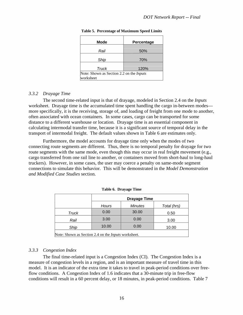
Freight carriers may not travel at the maximum speed at all times during travel. Thus, the model user has the opportunity to designate a more accurate representation of actual travel speeds for each mode, as shown in Table 5. The user can define a percentage; it may be the same across all three modes, or differentiated to reflect actual conditions such as traffic and capacity restrictions. Default values represent empirical information suggesting that trucks on I-95 travel faster than posted truck limits (similar to automobiles), that rail travels at slower average speeds due to community and crossing limits, and that ships operate near steady-state designed sea speeds. Adjustments made according to the maximum speed limit and the percentage of the maximum speed limit are calculated in Section 2.3 on the Inputs worksheet.

Table 4. State- and Port-Specific Speed Limits (mph)

State/Port Rail Ship Truck NY 70 50 NJ 70 55 PA 70 55 DE 70 55 MD 70 55 VA 70 55 NC 70 55 SC 70 60 GA 70 55 FL 70 65

NYC 25 PHL 25

WLM.DE 25 BLT 25 NFK 25

WLM.NC 25 CHL 25 SAV 25 JAX 25 OS 25

Notes: OS = Open Sea. Shown as Section 2.1 on the Inputs worksheet.


16

Table 5. Percentage of Maximum Speed Limits

Mode Percentage

Rail 50%

Ship 70%

Truck 120% Note: Shown as Section 2.2 on the Inputs worksheet

3.3.2 Drayage Time The second time-related input is that of drayage, modeled in Section 2.4 on the Inputs

worksheet. Drayage time is the accumulated time spent handling the cargo in-between modes—more specifically, it is the receiving, storage of, and loading of freight from one mode to another, often associated with ocean containers. In some cases, cargo can be transported for some distance to a different warehouse or location. Drayage time is an essential component in calculating intermodal transfer time, because it is a significant source of temporal delay in the transport of intermodal freight. The default values shown in Table 6 are estimates only.

Furthermore, the model accounts for drayage time only when the modes of two connecting route segments are different. Thus, there is no temporal penalty for drayage for two route segments with the same mode, even though this may occur in real freight movement (e.g., cargo transferred from one rail line to another, or containers moved from short-haul to long-haul truckers). However, in some cases, the user may coerce a penalty on same-mode segment connections to simulate this behavior. This will be demonstrated in the Model Demonstration and Modified Case Studies section.

Table 6. Drayage Time

Drayage Time

Hours Minutes Total (hrs)

Truck 0.00 30.00 0.50

Rail 3.00 0.00 3.00

Ship 10.00 0.00 10.00

Note: Shown as Section 2.4 on the Inputs worksheet.

3.3.3 Congestion Index The final time-related input is a Congestion Index (CI). The Congestion Index is a measure of congestion levels in a region, and is an important measure of travel time in this model. It is an indicator of the extra time it takes to travel in peak-period conditions over free-flow conditions. A Congestion Index of 1.6 indicates that a 30-minute trip in free-flow conditions will result in a 60 percent delay, or 18 minutes, in peak-period conditions. Table 7


17

shows the base Congestion Index for each node as provided by the Texas Transportation Institute’s 2005 Urban Mobility Study [Schrank and Lomax, 2005].11 Because the study did not provide an index for all the cities used in this model, cities without its own index values were assigned a substitute Congestion Index according to the nearest city of relative size with its own Congestion Index.

The default Congestion Index is included only for truck routes, but the user has the option of inserting a user-defined Congestion Index for any node and/or route segment, including those for rail and ship. This option is shown in Table 8. In the Peak Period? column, the user can designate whether or not the Congestion Index should be included in travel time calculations. If the value in Peak Period? is “1”, then the Average CI will calculate the average of the Congestion Index of the origin and destination nodes, but if and only if it is a truck route. If the value is zero, the travel time for that route segment will be calculated under free-flow conditions (i.e., the Congestion Index will not be used in optimization). In the User-Defined CI, the user can insert an alternate Congestion Index value for any route segment. In the Override Average CI? column, the user inserts a value of 1 if the user-defined Congestion Index value is preferred in travel time calculations. The Final CI column indicates the Congestion Index that will be used in actual travel time calculations. We note that congestion indices may change dramatically over time.

Table 7. Defining the Congestion Index for Each Node

Base Congestion Index (CI) Node Rail Ship Truck

NYC 0.00 0.00 1.43

PHL 0.00 0.00 1.36

WLM.DE 0.00 0.00 1.36

BLT 0.00 0.00 1.37

RCH 0.00 0.00 1.08

NFK 0.00 0.00 1.22

WLM.NC 0.00 0.00 1.18

FLO 0.00 0.00 1.06

CHL 0.00 0.00 1.18

SAV 0.00 0.00 1.18

JAX 0.00 0.00 1.17

Note: Shown as Section 2.5.1 on the Inputs worksheet.

11 Texas Transportation Institute names its congestion index the Travel Time Index (TTI). While we use TTI values in this study, users can input their own values; therefore, we use the more generic term Congestion Index.


18

Table 8. Defining the Congestion Index for Each Route Segment

Route ID Mode

Origin Node

Origin City

Dest. Node

Dest. City

Base CI inOrigin City

Base CIIn Dest.

City Peak

Period?*Average

CI

User-Defined

CI

OverrideAverage

CI?* Final

CI 1 Rail 1 NYC 2 PHL 0 0 1 0.00 0 0 1.002 Truck 1 NYC 2 PHL 1.43 1.36 1 1.40 0 0 1.403 Ship 1 NYC 6 NFK 0 0 1 0.00 0 0 0.004 Ship 1 NYC 7 WLM.NC 0 0 1 0.00 0 0 0.005 Ship 1 NYC 9 CHL 0 0 1 0.00 0 0 0.00

* 1=yes, 2=no. Note: Shown as Section 2.5.2 on the Inputs worksheet

3.4 Data Relevant to Travel Cost

3.4.1 Rate-per-Mile The first cost-related input is the rate-per-mile (RPM) for each mode, as shown in Table

9. The RPM is an often-used cost measure in freight transportation. The RPM may be specified differently for each mode. We use a consistent RPM for each mode, and do not adjust for different freight types or different locations throughout the East Coast. This was also supported by the data we received as discussed below.

Table 9. Rate-per-Mile ($/mile)

Mode RPM

Truck $1.73

Rail $1.09

Ship $1.12 Note: Shown as Section 3.1 on the Inputs worksheet

RPM data were extracted from a 2006 report that examined the market viability of short-sea shipping on four traffic corridors, including the Atlantic Coast corridor, the Gulf of Mexico to the Atlantic Coast corridor, Pacific Coast corridor, and the Great Lakes corridor [Global Insight Inc. and Reeve & Associates, 2006]. The study produced a shipper cost per highway mile for truck, intermodal rail, and status quo as well as “best in class” short-sea shipping rates for all four corridors. For purposes of this case study, truck, rail, and status quo short-sea rates attributed to North/South Atlantic transportation were used. Users may input different RPM values based on the type of transportation technologies and study regions.

3.4.2 Drayage Cost Another cost component in travel cost calculation is drayage cost, which is the cost of an

intermodal cargo transfer from one mode to another. The cost of drayage is separate from the


19

actual shipping cost, and is generally consisted of fuel surcharges, waiting time (i.e., time the container is at rest and waiting to be moved), access charges, labor, and other cost factors. Additionally, the structure of the drayage rate may vary by the freight company offering the service, and by local unions. Default drayage cost is displayed in Table 10. The user has the ability to modify these costs as appropriate for the case being studied.

Table 10. Drayage Cost in $/TEU-transfer

Ending Mode ($/TEU)

Starting Mode Rail Ship Truck

Rail $0 $105 $225

Ship $105 $0 $105

Truck $225 $105 $0 Note: Shown as Section 3.2 on the Inputs worksheet

In a report titled Cross Border Short-sea Shipping Study, conducted by Cambridge Systematics, Inc. [2007], the drayage rates, inclusive of fuel surcharges, were collected for short-sea shipping carriers in the Cascades region of the U.S. Pacific Northwest and Canada. These rates were used as the drayage rates for truck-ship and ship-truck service in the model. The source of ship-rail and rail-ship drayage rates is a report titled, Inland Port Feasibility Study. This report encompassed a market analysis of intermodal transportation, particularly between ships and rail, in the San Joaquin Valley and the Port of Oakland, CA [Tioga Group Inc. et al., 2003]. With respect to truck-rail and rail-truck drayage rates, specific data were not available, so an estimate was used.

3.4.3 Cost Factors in Intermodal Transportation The cost system is inherently complex and sensitive to market changes. Some of the

costs of intermodal transportation include [Plauche]:

- Variable Costs: o Lift costs (the cost of lifting freight on and off a train within a terminal.) o Fuel costs

- Fixed Costs: o Maintenance of way (track) costs o Costs of risk (damaged lading) o Rail car costs o Crew costs (engineers and conductors to drive the train) o Locomotive costs (ownership and maintenance costs) o Terminal switching

- Depreciation

Additionally, the breakdown of costs of supplying transportation of freight to a customer is rarely made available. Thus, this model does not attempt to incorporate each of these elements,


20

but instead use an all-inclusive cost that is representative of all the fixed and variable costs. Providing an all-inclusive cost to customers is customary in the industry. For this reason, the model incorporates a single cost factor for each of three modes; this cost factor is assumed to be on a per-mile basis, and can be altered by the user.

3.5 Data Relevant to Emissions Emissions data were collected from a variety of sources, including two transportation-

related models. The first model, developed in 1995 by the U.S. Department of Energy’s Office of Transportation Technologies and Argonne National Laboratory, is the GREET model. GREET is an analytical tool that estimates total fuel-cycle energy use and emissions associated with transportation technologies and fuels [Wang, 2001]. The second model used was the Total Energy & Emissions Analysis for Marine Systems (TEAMS) model, developed in 2005 by James J. Winebrake, Ph.D. and Patrick E. Meyer of Rochester Institute of Technology, and James J. Corbett, Ph.D. of the University of Delaware, in sponsorship by the Research and Special Programs Administration (now the Research and Innovative Technology Administration) under the U.S. Department of Transportation. TEAMS is similar to GREET, with the exception that it calculates total fuel-cycle emissions and energy consumption for marine systems, including ferry boats and container ships.

In the model inputs worksheet, emission factors are input in grams per TEU-mile.12 However, we found that emission factors may not always be provided in those units. Thus, the emission factors for rail, ship, and truck are calculated differently, as shown in Table 11. The GREET model, from which rail and truck emission factors were derived, were provided in grams per million Btu (mmBtu). GREET also provided the Btu/ton-mile for a typical container via rail. Included with a pre-determined tonnage per TEU, the model converts the emission factor into units of grams per TEU-mile. The inclusion of tons per TEU enables the consideration of different weights carried per TEU—because they are not always the same, depending on the goods being carried, and the mode on which it is transported.

Lastly, Table 12, also in Section 4.2, shows a summary of all emission factors are consolidated into a single table. The values displayed here are important, not only because they are derived from the calculations in the previous, but also because they are used in optimization of emissions. Both models were used to extract emissions factors for VOC, CO, NOx, PM, SOx, and CO2. Given the global nature of CO2 and the local/regional nature of our other pollutants, we use total fuel cycle emissions for CO2 and simple end-use (tailpipe, engine stack, or vessel stack) emissions for all other pollutants.

Emissions factors were collected in units of grams per TEU-mile. This is a measure of the emissions output for each mile one TEU is transported.

12 A TEU, or twenty-foot equivalent unit, is a common defined container unit for shipping cargo, and at its standard, it is 20 feet long, 8'6" feet high and 8 feet wide. However, container sizes have increased to accommodate the need to ship more freight across longer distances. In this model, the standard dimensions of a TEU are considered.


21

Table 11. Emission Factors and other Designates

Rail Designations

Pollutant g/mBtu Btu/ton-mi tons/TEU g/TEU-mi VOC 73 370 5.0 0.14 CO 213 370 5.0 0.39 NOx 1,517 370 5.0 2.81 PM10 36 370 5.0 0.07 SOx 17 370 5.0 0.03 CO2 78,363 370 5.0 144.97

Ship Designations Pollutant grams/ship-mi TEU/ship g/TEU-mi VOC 1,493 5,000.0 0.30 CO 6,869 5,000.0 1.37 NOx 39,626 5,000.0 7.93 PM10 1,173 5,000.0 0.23 SOx 19,559 5,000.0 3.91 CO2 1,464,151 5,000.0 292.83

Truck Designations

Pollutant g/mBtu TEU/truck g/TEU-mi VOC 0.68 2.0 0.34 CO 3.27 2.0 1.64 NOx 13.73 2.0 6.86 PM10 0.24 2.0 0.12 SOx 0.44 2.0 0.22 CO2 2,002 2.0 1,001.00

Note: Shown as Sections 4.1.1, 4.1.2, and 4.1.3 on the Inputs worksheet

Table 12. Summary of Emission Factors (g/TEU-mi)

Pollutant Mode VOC CO NOx PM10 SOx CO2 Truck 0.34 1.64 6.86 0.12 0.22 1,001.00 Rail 0.14 0.39 2.81 0.07 0.03 144.97 Ship 0.30 1.37 7.93 0.23 3.91 292.83

Note: Shown as Section 4.2 on the Inputs worksheet


22

3.6 Freight Data The last data component on the Inputs worksheet is that of the quantity of TEU containers

being shipped, shown below in Table 13. Emissions quantities are calculated in units of TEUs per mile, so it is necessary to clarify the number of actual containers being shipped. The default value is “1”. This ensures that a truck can be assigned the cargo in all optimization runs; the model therefore implicitly assumes that capacity in rail or shipping will be met by other freight so that a larger train is not assumed to move 1 TEU only.

Table 13. Quantity of TEU Containers

TEUs

All Modes 1 Note: Shown as Section 5.1 on the Inputs worksheet

4 The Model: Using Solver

4.1 Overview At the core of this model is Solver, an optimizing agent bundled with Microsoft Excel.

While the model will run with the standard Excel-based Solver add-in, we also tested the model using Premium Solver— an advanced version of the standard Excel Solver— that is available for purchase. Solver is able to perform optimization on many types of spreadsheet models, including non-linear, linear, and discontinuous functions. Premium Solver can handle up to 500 decision variables and 250 constraints in a smooth nonlinear model [Frontline Solvers, 2006]. With Premium Solver, it is possible to significantly expand the current version of the model for more specialized analysis; with standard Excel Solver Add-in, the tool still works for simple networks. This report assumes that the user has some working understanding of optimization modeling and the Excel Solver add-in.

4.2 Elements of the Solver Worksheet The Solver’s purpose is to find the best—or optimal— solution with the variables it is

given. The optimal solution is one that either maximizes or minimizes an objective function and satisfies given constraints [Frontline Solvers, 2006]. In this model, Solver optimizes for eight separate objectives: travel time, travel cost, and six different pollutant emissions. For each objective, the Solver must solve for the optimal combination of route segments—which are the decision variables in the model—that minimizes the objective function (e.g., least cost, least travel time, least emissions) in a complete trip from New York City to Jacksonville (or other origin-destination provided by the user). Furthermore, the Solver must satisfy certain constraints discussed in more detail in the following sections.

The Solver worksheet is divided into five main sections. Each section has a set of columns, each with its own function. The components of these sections are shown in Table 14.


23

Table 14. Components of the Solver Worksheet and their Functions

Category Function Route Selection

Select_Route? Indicates whether or not the route segment is selected. A value of 1 indicates the segment is selected, and 0 otherwise. The cells in this column are referred to as the decision variables.

Route Data Route Characteristics Provides information about route segments.

Route ID Numerical reference for each route segment, consisting of the mode, origin node, and destination node. The values in this column are the only values in the entire sheet that are entered manually.

Mode Indicates the mode used in the route segment. Orig_Node Indicates the node of origin. Orig_City Indicates the name of the origin city. Dest_Node Indicates the destination node. Dest_City Indicates the name of the destination city.

Distances Provides distance information for route segments. Orig_State Indicates the name of the state in which the origin resides. For ship routes, this refers to the

distance between the origin port and the boundary to the open sea. Dest_State Indicates the name of the state in which the destination resides. For ship routes, this refers

to the distance between the boundary of the open sea and the destination port. Thru_State Indicates the state that lies between the origin and destination states. This mostly applies to

ship routes, as it indicates the distance on the open sea. Travel Time Zone Identification This section provides information about route segments that are used in the Base Travel

Time calculations. Orig_State Indicates the origin state in the route segment. Dest_State Indicates the destination state in the route segment. Thru_State Indicates the through state in the route segment. For ship routes, it indicates whether a

portion of the route segment is spent on the open sea. Preliminary Travel

Time This section is where preliminary travel time calculations are performed. Preliminary travel time is measured in hours and does not include the travel time index and drayage times. Also, the preliminary travel time is only calculated for the mode indicated in the Route Data category.

Rail Calculates the preliminary travel time spent on the corresponding route segment via rail. Ship Calculates the preliminary travel time spent on the corresponding route segment via ship. Truck Calculates the preliminary travel time spent on the corresponding route segment via truck.

Congestion Index Indicates the final Congestion Index (CI) as determined on the Inputs sheet. Drayage Time Obtains the drayage time for each mode as determined in Section 2.4 of the Inputs sheet.

Drayage time is retrieved only for the mode indicated in the corresponding route segment. Drayage time is measured in hours.

Rail Indicates the drayage time for the corresponding route segment via rail. Ship Indicates the drayage time for the corresponding route segment via ship. Truck Indicates the drayage time for the corresponding route segment via truck.

Total Travel Time Calculates the total travel time of a route segment. Base Calculates the preliminary travel time and the CI, and is used in calculating the total travel

time. Rail Drayage Calculates the drayage time if an intermodal switch is made to rail. Ship Drayage Calculates the drayage time if an intermodal switch is made to ship. Truck Drayage Calculates the drayage time if an intermodal switch is made to truck. Total Calculates the total travel time of the route segment by summing the base travel time with

the drayage time associated with an intermodal switch, if one does occur. This column, in conjunction with the Route Selection column, is used by the Solver to optimize travel time.


24

Category Function Travel Cost Calculations Drayage Cost Obtains the cost of drayage for each mode as determined in Section 3.2 of the Inputs sheet.

Drayage cost is retrieved only for the mode indicated in the corresponding route segment. Drayage cost is measured in dollars per intermodal switch from the primary mode to the secondary mode.

Switch to Rail Cost of switching from the primary mode to rail. Switch to Ship Cost of switching from the primary mode to ship.

Switch to Truck Cost of switching from the primary mode to truck. Segment Cost Calculates the base and total segment cost for each route segment.

Base Obtains from Section 3.1 of the Inputs sheet the rate-per-mile (RPM) for the mode indicated in the segment, and multiplies it with the total segment distance.

Rail Drayage Indicates the drayage cost for the corresponding route segment via rail. Ship Drayage Indicates the drayage cost for the corresponding route segment via ship. Truck Drayage Indicates the drayage cost for the corresponding route segment via truck.

Total Calculates the total segment cost by summing the base segment cost with the drayage cost associated with an intermodal switch, if one does occur. This column, in conjunction with the Route Selection column, is used to optimize travel cost.

Emissions Calculations Base Emissions Obtains the product of the emission factor for the segment mode, the TEU specified in

Section 5.1 of the Inputs sheet, and the total distance for the segment. Emissions for each pollutant are given in units of grams emitted per TEU-mile. The Solver uses each of these five columns, in conjunction with the Route Selection column, to optimize for individual pollutant emissions.

VOC Total emissions for the pollutant VOC. CO Total emissions for the pollutant CO. NOx Total emissions for the pollutant NOx. PM Total emissions for the pollutant PM. SOx Total emissions for the pollutant SOx. CO2 Total emissions for the pollutant CO2.

Calculating Intermodal Switches (this section is hidden from view on the Solver worksheet) First Mode Indicates the mode used in the primary route segment if the route segment is selected (has a

value of 1 in the Select Route? column). If the route segment is not selected (has a value of 0), then the cell returns a value of 0.

Second Mode Indicates whether the First Mode is equal to zero; if it does, then it means the route segment is not selected so the cell returns a value of zero; otherwise, it returns the First Mode value.

Switch? Identifies whether or not the Second Mode is equal to the mode used in the route segment in the above route segment (one row above), and returns a value of zero to indicate no intermodal switch; otherwise, it returns a value of 1.

Intermodal Switches

Sums up the Switch? column to indicate the total number of intermodal switches.

4.3 Calculating Travel Time The total travel time from origin to destination is calculated as the sum of the travel times

of individual route segments linking origin and destination. The travel time of a given origin-destination route is calculated as the product of the base travel time ti,m for each segment i and Xi,m, the binary variable representing the route segment’s selection by the model, added by the drayage time Dm,i for the mode used in segment i. The equation for this is shown below.


25

Equation 1. Calculation of Total Travel Time for Selected Route Segments

( )∑ +⋅=mi

mimimi DtXT,

,,,

Where:

T Is the total travel time of the origin-destination route. Xi,m Is a binary variable equal to “1” if route segment i is selected using mode m, and “0” otherwise. ti,m Is the base travel time in route segment i using mode m. Di,m Is the drayage time of the mode m used in route segment i.

The equation to calculate the base travel time ti,m is shown in Equation 2. The base travel time for a given route segment is the sum of the travel time within each travel zone, multiplied by the Congestion Index (CIm,i) for the mode used in route segment i.

Equation 2. Calculation of the Base Travel Time for a Route Segment

zimz z

zmimi CI

kd

t ,,,,

, ⋅⎟⎟⎠

⎞⎜⎜⎝

⎛=∑

Where: z Is the set of travel zones {1, 2, 3} where 1=origin state/origin RSZ, 2=destination state/destination

RSZ, and 3=through-state/open sea. di,m,z Is the distance of route segment i, using mode m in zone z.

kz Is the travel speed used in travel zone z. CIm,i,z Is the Congestion Index of mode m used in route segment i, zone z.

The equation to calculate drayage time Di,m is shown in Equation 3. The drayage time for a given route segment is zero if the mode mi-1 used in the first segment is the same as the mode mi used in the next segment. This indicates that no intermodal switch has occurred. However, an intermodal switch has occurred if mi-1 is not equal to mi. In this case, the drayage time for the first route segment (Dm,i-1) is applied if Xi-1,m and Xi,m (the binary decision variables indicating whether the route segments i-1 and i have been selected), both equal 1.

Equation 3. Calculation of Drayage Time for a Given Mode in a Route Segment

If ii mm =−1 , then 0, =miD

If ii mm ≠−1 , then imiimi XDXDii⋅⋅=

−−− 1,11,

Where: Di,m Is the drayage time for mode m used in route segment i. mi-1 Is the mode m used in the first route segment (i-1). mi Is the mode m used in the second route segment (i). Xi-1 Is a binary variable equal to “1” if the first route segment is selected, and “0” otherwise. Xi Is a binary variable equal to “1” if the second route segment is selected, and “0” otherwise.


26

4.4 Calculating Travel Cost The equation for the total travel cost of all selected route segments is calculated as the sum

of the costs of individual, selected, route segments. The equation for this is shown below.

Equation 4. Calculation of Total Travel Cost for All Selected Route Segments

( )∑ +⋅=mi

mimimi WJXU,

,,,

Where: U Is the total travel cost of the route from origin to destination.

Xi,m Is a binary variable equal to “1” if route segment i is selected my mode m, and “0” otherwise. Ji,m Is the base travel cost of route segment i by mode m in dollars. Wi,m Is the drayage cost of mode m used in the route segment in dollars.

The base travel cost for a given route segment, Ji,m, is represented by the equation:

Equation 5. Calculation of the Base Travel Cost for a Route Segment

mimimi dAJ ,,, ⋅=

Where: Ai,m Is the rate per mile A of the mode m used in route segment i. di,m Is the distance in segment i using mode m.

Furthermore, the drayage cost Wi,m is calculated according to Equation 6 similar to the drayage time discussed above. Drayage time is applied only if the mode used in one route segment is different than the mode used in the next route segment.

Equation 6. Calculation of Drayage Cost for a Given Mode in a Route Segment

If ii mm =−1 , then 0, =miW

If ii mm ≠−1 , then imiiimi XWXWi⋅⋅=

−−− 1,11,

Where: Ws,m Is the drayage cost for mode m used in segment s. m1 Is the mode m used in the first route segment. m2 Is the mode m used in the second route segment. C1 Is a binary variable equal to “1” if the first route segment is selected, and “0” otherwise. C2 Is a binary variable equal to “1” if the second route segment is selected, and “0” otherwise.


27

4.5 Calculating Pollutant Emissions For emissions, the calculation for each of the six pollutants is shown in the equation below.

Equation 7. Calculation of Emissions

( )∑ ⋅⋅⋅=mi

mimimnn XdwEFE,

,,,

Where: En Is emissions of pollutant type n in grams.

EFn,m Is the emission factor of pollutant n used with mode m in grams/TEU-mile. w Is the quantity of TEUs being transported.

di,m Is the distance traveled by mode m along segment i in miles. Xi,m Is a binary variable equal to “1” if segment i is selected by mode m, and “0” otherwise.

4.6 Formulae in Optimization Columns The Total Travel Time, Total Segment Cost, and all six of the emissions optimization

columns have their own unique formulae that are sensitive to changes. In each column, the cells are uniquely set up so that they all direct to the same group of possible secondary route segments. This is because the destination node in the primary segment becomes the origin node in the secondary segment. Therefore, care should be exercised in ensuring that these formulae direct to the correct cells; otherwise, the Solver will not evaluate all segment options that are actually available. This is the reason why the route segment list on the Solver worksheet is not listed in order by Route_ID, but instead by, first, the Orig_Node, the mode, and then the Dest_Node. If the order of this route list is altered, the formulae in each of the cells within the Total Travel Time and Total Segment Cost columns will not direct to the correct decision variables in the Route_Select? column, and thus will be incorrect.

4.7 Defining the Constraints in a Network Flow Model

4.7.1 Net Flow Constraints In a network flow model such as this one, there is a balance between supply and demand

at each node. Node 1, which is the node for NYC, has a supply of 1, and node 11 (JAX) has a demand of –1 (illustrated in Table 15) All the other nodes that lie between nodes 1 and 11 have a value of 0. Recall that each route segment, or arc, is a connection between two nodes. This instructs the model that the net flow (inflow - outflow) at each node must be equivalent to its supply or demand. In other words, each network flow constraint indicates that the flow into a given node less the flow out of that same node must be equal to the supply or demand at that node. Thus, the Solver is required to optimize for an objective by choosing the most optimal route that begins with node 1 (NYC), and ends at node 11 (JAX), and for all other nodes, there must be an incoming and an outgoing arc at that node. The mathematical structure of each arc constraint is shown below in Table 16.

Suppose after running the mode for travel time minimization, the Solver chose the trip layout shown in Table 17. All the node constraints would be satisfied. Net flow at node 1 equals (-1), satisfying the node 1 constraint. Net flows at nodes 2 and 10 equal zero, satisfying node 2 and 10 constraints. And net flow at node 11 equals 1, satisfying the node 11 constraint. Thus, maintaining the balance of flow in these constraints is imperative in ensuring the effectiveness of


28

the model. This ensures that the Solver always chooses a combination of routes, or arcs, that have the origin and destination nodes as specified by the model user. The user can change the origin and destination points of the model by placing a (-1) at the origin and a (+1) at the destination, with zeroes (0) at all other nodes.

Table 15. Network Flow Constraints

Node Net Flow Supply/Demand1 0 -1 2 0 0 3 0 0 4 0 0 5 0 0 6 0 0 7 0 0 8 0 0 9 0 0

10 0 0 11 0 1

Table 16. Mathematical Representation of Net Flow Constraints

Constraint Mathematical Representation Node 1 -X12 – Y16 – Y17 – Y19 – Y1,10 – Y1,11 – Z12 = -1 Node 2 +X23 + Y26 + Y27 + Y29 + Y2,10 + Y2,11 + Z23 – X12 – Z12 = 0 Node 3 +X34 + Y36 + Y37 + Y39 + Y3,10 + Y3,11 + Z34 – X23 – Z23 = 0 Node 4 +X45 + Y46 + Y47+ Y49 + Y4,10 + Y4,11 + Z45 – X34 – Z34 = 0 Node 5 +X56 + X57 + X58 + Z56 + Z57 + Z58 – X45 – Z45 = 0 Node 6 +X68 + Y67 + Y69 + Y6,10 + Y6,11 + Z68 – X56 – Y16 – Y26 – Y36 – Y46 – Z56 = 0 Node 7 +Z79 + Z7,10 + Z7,11 – X57 – Y17 – Y27 – Y37 – Y47 – Y67 – Z57 = 0 Node 8 +X89 + Z89 + Z8,10 – X58 – X68 – Z58 – Z68 = 0 Node 9 +X9,10 + Y9,10 + Y9,11 – X89 – Y19 – Y29 – Y39 – Y49 – Y69 – Y79 – Z89 = 0 Node 10 +X10,11 + Y10,11 + Z10,11 – X9,10 – Y1,10 – Y2,10 – Y3,10 – Y4,10 – Y6,10 – Y7,10 – Y9,10 – Z8,10 = 0 Node 11 -X10,11 – Y1,11 – Y2,11 – Y3,11 – Y4,11 – Y6,11 – Y7,11 – Y9,11 – Y10,11 – Z10,11 = 1

Notes: X = arc assigned to rail mode; Y = arc assigned to ship mode; Z = arc assigned to truck mode. Each arc takes on a value of 1 or 0, depending on whether it is selected by the Solver. The subscript numerals refer to the origin and destination nodes in that particular arc. For instance, X12 indicates an arc from node 1 to node 2 via rail. Similarly, Z2,11 indicates an arc from node 2 to node 11 via ship.

Table 17. Example Trip Layout

Select Route? (1=yes 0=no)

Route_ID Mode

Orig_ Node

Orig_ City

Dest_ Node

Dest_ City

1 1 Rail 1 NYC 2 PHL 1 13 Ship 2 PHL 10 SAV 1 52 Truck 10 SAV 11 JAX


29

4.7.2 Binary Constraints Another constraint vital to the effectiveness of the model is the binary constraint, of

which is placed on the decision variables. The binary constraint enforces the restriction of the changing cells to a value of either “1” or “0”, essentially acting as an “on/off” switch that shows whether a route segment has been selected or not.

4.7.3 The Constraints as Shown on the Solver Parameters Dialog In any optimization run, the Solver Parameters Dialog should contain the constraints

previously discussed, and they should be in the format shown in Figure 7. The first constraint indicates that all the decision cells must be binary. The second constraint instructs the model that the value of each node in the Net Flow column must be equal to that in the Supply/Demand column (refer to Table 15).

Figure 7. Example Solver Parameters Dialog Box

4.7.4 A Note About Solver Engines There are several options for solver algorithms. Three Premium Solver engines are

available for use: the Standard GRG Nonlinear engine, the Standard Simplex LP engine, and the Standard Evolutionary engine (see Figure 7). When travel time or travel cost is the objective

Premium Solver EnginesConstraints

Time and Cost optimization option settings; for Emissions, select “Assume Linear Model”


30

being optimized, the Standard GRG Nonlinear engine must be used. If using standard Excel Solver, one must deselect the “Assume Linear Model” under the Options button to solve for travel time and travel cost (also shown in Figure 7). This is because the drayage functions make these calculations nonlinear. Alternatively, the Standard Simplex LP engine must be used in emissions optimization; if in the future, drayage penalties are added to emissions, then that model will become nonlinear as well.

4.8 Solver Results After a simulation run, the Solver will produce results in the form shown in Table 18. The

first row indicates the values obtained in the current optimization. In addition to showing the optimal value for the optimized objective, it also shows the values for the other variables. The Target (Optimal) Solution shows the most optimal solution for the objective in that column (for the default case discussed here). The Deviation from Optimal is a percentage value that shows the percentage change between the current optimal solution and the single-constraint solution. Note that if the user modifies the network structure, chooses other origin-destination points, or changes any input data, they should run the model again for each objective and place those values in the Single-Constraint Solution cells. Lastly, the Intermodal Switches cell indicates the number of intermodal switches that take place in the route layout that produced the current optimal solution.

Table 18. Example Optimization Results

Solver Results Time Cost VOC CO NOx PM SOx CO2 Current Optimal Solution 24 1,424 334 1,572 6,765 120 210 946,815Single-Constraint Solution 17 954 127 367 2,613 62 30 134,969Deviation from Optimal 41% 49% 162% 328% 159% 93% 605% 602% Intermodal Switches 2 Note: Units are i) Time (hours); ii) Cost ($); iii) emissions (grams); solver results are rounded from Excel output for presentation.

5 Model Demonstration and Modified Cases

5.1 Comparison of the Top Three Optimal Solutions for Each Objective To demonstrate the capabilities of the model, the model was run for each of the eight

objectives with the goal of minimizing each objective—time, cost, and each of the six pollutants—to obtain the most optimal values for each. Next, each objective was optimized to retrieve the second most optimal solution. A third run was also done. Retrieving the top three most optimal solutions allows for the evaluation of differences in time, cost, and emissions.

To conduct this analysis, the optimal solution is used as a constraint in the second optimization run; the purpose is to force the second most optimal value to be a value greater than the optimal solution. However, in the version of Solver used for this model, it is necessary to manually input the limit. For example, if the optimal solution for a given objective were 15.11,


31

then the constraint in the second run would be that the objective value must be greater than or equal to 15.1213. This approach was also used in third-best-solution optimizations.

All the results from the first, second, and third most optimal solutions are listed by objective on the Simulation_Results worksheet. Figure 8 displays the percentage deviations from the most optimal solution for the 2nd and 3rd optimal solutions using single-constraint objectives. For instance, when travel cost was optimized, the optimal cost value was $954 for a trip from New York City to Jacksonville. The 2nd optimal solution is ~13% higher at $1,080, and the 3rd optimal is ~31% higher, at $1,246. The difference between the 2nd and 3rd solutions is ~17%. In the case of PM emissions, the 2nd optimal solution produced 65 grams of emissions per TEU-mile, or ~5% more than the optimal amount of 61.9 g/TEU-mi, and in the 3rd optimal solution, the amount emitted is ~10% more than the optimal amount, or about double the second best solution.

Thus, a transportation planner can derive from this model a better understanding of the differences in payoffs between optimal solutions. That is to say, if the objective were to minimize PM emissions, but taking the most optimal route is not possible, then a satisfactory choice between the second and third optimal route may be left to other decision factors, such as cost.

Figure 8. Comparison of the 2nd and 3rd Optimal Solutions to the Optimal within Each Measured Output

Comparison of the 2nd and 3rd Optimal Solutions to the Most Optimal within Each Objective

8%

14%

8%5%

31%

11%

22%

11% 10%

24% 24%

13%

22%

28%

22%

41%

0%5%

10%

15%20%25%30%35%

40%45%50%

Time Cost VOC CO NOx PM SOx CO2

Dev

iatio

n fro

m

Opt

imal

Val

ue (%

)

2nd Optimal 3rd Optimal

Figure 9 compares the top-three optimal solutions minimizing each output parameter with single-constraint solutions across all objectives. Where Figure 8 provides insight into how the best outcome compares within a constraint to its second and third best outcomes, Figure 9

13 In the version of Solver used for this model, the options of equality signs are limited to greater/less than or equal to, or equal to signs. Greater/less than signs are not available, so the constraint value must be manually entered as being greater than the value in the previous run.


32

provides insights into how the best three constraints for one measure differs across other measures from an optimal outcome. This shows, for example, that the best time routes can produce twice (or more) the emissions of the lowest polluting routes; conversely, the lowest polluting routes tend to require significantly more travel time. It also shows that the least-cost routes perform similarly in terms of time and emissions tradeoffs.

5.2 Modified Case Study A: Imposing Drayage Cost Penalties on Same-Mode Route Connections

To provide more insight into other model uses, we developed a modified case that considers the effects of same-mode node penalties (cost, energy, etc.) on the optimal routes. In the drayage cost modification, assume that a short-haul freight carrier and long-haul freight carrier exchange cargo at a single-mode transfer terminal (e.g., truck transfer facility). This could involve a cost penalty on two connecting route segments that share the same mode.

Drayage costs may produce differences in cost, time, and the overall route layout. In the altered scenario, two outcomes may be expected: (1) the route selected is a single leg from origin to destination, or (2) two or more route segments with intermodal switches will be selected. Drayage cost for same-mode connections can be assigned a penalty value for each mode in Section 3.2 of the Inputs worksheet. For illustration purposes only, drayage costs were assigned arbitrarily; rail-rail connections were assigned a cost of $250, ship-ship transfers were set $400, and a cost of $375 for truck-truck connections.14 With these input changes, the model was run again. In the cost-optimal case, the total trip cost was $953.79, as highlighted in Table 19 below. This trip consisted of an all-ship route with a connection in WLM.NC, as shown in Table 20.

Table 21 and Table 22 show the new cost optimal value, which was indeed a single route segment via ship from NYC to JAX, with a total cost of $997, a difference of $43, or a 4.5% increase from the cost-optimal case. The comparison between the cost-optimal scenario and a second- or third-best result may be sufficient information for the freight carrier to make a decision; if not, more simulations may be done to evaluate other solutions. This can be done by placing a constraint on travel cost so that the objective function value must be greater than or equal to $997.15

5.3 Modified Case Study B: Seeking Alternate, Less Congested Routes In freight transportation planning, avoiding congested areas is a top priority. With this

model, it is possible to use time optimization to seek alternate routes according to geographical location, mode used, and by time period. Section 2.5 on the Inputs sheet, which contains information regarding the Congestion Index, is where data on congestion factors are input. In this case study, we assume that a freight carrier has received Congestion Indices for rail and ship modes, and for all 11 nodes. The CI data are given in Table 23.

14 Further research or additional data would be required to determine the actual costs and conditions under which these may apply. That data was not available for this study, and is beyond the scope. 15 Recall that in assigning constraint values, the value must be slightly larger or less than the optimal value. If the constraint value is the same as the optimal solution in the prior case, then the Solver will result in the same answer.


33

Figure 9. Comparison of 1st, 2nd and 3rd Optimal Solutions to Single-constraint Solutions across Other Measures

Comparison of the Top Three Optimal Solutions for Travel Cost Across Other Optimal Constraints

1%

10%

100%

1000%

10000%

100000%


Objective

Dev

iatio

n fr

om

Opt

imal

Res

ults

(%)

Cost Optimal 2nd Cost Optimal 3rd Cost Optimal

Comparison of the Top Three Optimal Solutions for VOC Emissions Across Other Optimal Constraints

0%

50%

100%

150%

200%


Objective

Dev

iatio

n fr

om

Opt

imal

Res

ults

(%)

VOC Optimal 2nd VOC Optimal 3rd VOC Optimal

Comparison of the Top Three Optimal Solutions for CO Emissions Across Other Optimal Constraints

0%

50%

100%

150%

200%

250%


Dev

iatio

n fr

om

Opt

imal

Res

ults

(%)

CO Optimal 2nd CO Optimal 3rd CO Optimal

Comparison of the Top Three Optimal Solutions for NOx Emissions Across Other Optimal Constraints

0%

50%

100%

150%

200%


Dev

iatio

n fr

om

Opt

imal

Res

ults

(%)

NOx Optimal 2nd NOx Optimal 3rd NOx Optimal

Comparison of the Top Three Optimal Solutions for PM Emissions Across Other Optimal Constraints

0%

50%

100%

150%

200%


Dev

iatio

n fr

om

Opt

imal

Res

ults

(%)

PM Optimal 2nd PM Optimal 3rd PM Optimal

Comparison of the Top Three Optimal Solutions for SOx Emissions Across Other Optimal Constraints

0%

50%

100%

150%

200%

250%


Dev

iatio

n fr

om

Opt

imal

Res

ults

(%)

SOx Optimal 2nd SOx Optimal 3rd SOx Optimal

Comparison of the Top Three Optimal Solutions for CO2 Emissions Across Other Optimal Constraints

0%

50%

100%

150%

200%

250%


Dev

iatio

n fr

om

Opt

imal

Res

ults

(%)

CO2 Optimal 2nd CO2 Optimal 3rd CO2 Optimal

Comparison of the Top Three Optimal Solutions for Travel Time Across Other Optimal Constraints

0%100%200%300%400%500%600%700%


Objective

Dev

iatio

n fr

om

Opt

imal

Res

ults

(%)

Time Optimal 2nd Time Optimal 3rd Time Optimal


34

Table 19. The Original Cost Optimal Solution


hours/trip $/trip g/TEU-mig/TEU-mig/TEU-mig/TEU-mi g/TEU-mig/TEU-miCurrent Optimal Solution 49 954 254 1,170 6,749 199 3,331 249,374 Single-Constraint Solution 17.06 953.79127.36 367.43 2,612.99 61.90 29.73 134,968 Deviation from Optimal 186.5% 0.0% 99.7% 218.4% 158.3% 222.9% 11105.3%84.8% Intermodal Switches 0

Table 20. The Original Cost Optimal Solution: Route Selection

Select Route? (1=yes 0=no) Route_ID Mode

Orig_Node

Orig_ City

Dest_ Node

Dest_ City

1 4 Ship 1 NYC 7 WLM.NC 1 43 Ship 7 WLM.NC11 JAX

Table 21. Drayage Cost Altered Case: The New Optimal Solution


hours/trip $/trip g/TEU-mi g/TEU-mi g/TEU-mi g/TEU-mi g/TEU-mi g/TEU-mi Current Optimal Solution 38 995 264 1,215 7,001 207 3,437 261,494 Target (Optimal) Solution 17.06 953.79 127.36 367.43 2,612.99 61.90 29.73 134,968 Deviation from Optimal 120.3% 4.4% 107.5% 230.6% 167.9% 234.3% 11459.8% 93.7% Intermodal Switches 0

Table 22. Drayage Cost Altered Case: Route Selection

Select Route? 1=yes, 2=no Route_ID Mode Orig_

NodeOrig_City

Dest_Node

Dest_ City

1 7 Ship 1 NYC 11 JAX

Furthermore, the freight carrier has received real-time data showing severe congestion in the Delaware area on highways and ports. Causes of congestion are outside the model scope, but could be due to seasonal tourism, timing of the route to coincide with commuting, etc. The freight carrier has decided to avoid ship and truck routes that involve that region.

The new CI data was thus inserted in Section 2.5.1 on the Inputs sheet, and the Peak Period? option (in Section 2.5.2) was turned on at all route segments, so the Average CI was used to calculate the travel delay incurred during that route segment. The final step prior to running the model under these new conditions is inserting new constraints on all the decision variables that correspond to route segments where Wilmington, Delaware is either the origin or destination. These constraints as entered in the Solver Parameters Dialog are shown in Figure 10 below.


35

The resulting time optimal value was ~35 hours, representing a ship from New York to Savannah and trucking from there to Jacksonville. The Solver results are shown in Table 24 and Table 25.

Table 23. Congestion Index (CI) Selections for Case Study 2

Node Rail Ship

NYC 1.76 1.83

PHL 1.54 1.48

WLM.DE 1.2 1.35

BLT 1.34 1.45

RCH 1.27 N/A

NFK 1.71 1.39

WLM.NC 1.40 1.33

FLO 1.15 N/A

CHL 1.43 1.36

SAV 1.22 1.55

JAX 1.39 1.67

Figure 10. Constraints Used in Case Study 2

Table 24. Optimization Results for Case Study 2

Time Cost VOC CO NOx PM SOx CO2 hours/trip $/trip g/TEU-mi g/TEU-mi g/TEU-mi g/TEU-mi g/TEU-mi g/TEU-mi

Current Optimal Solution 35 1,124 277 1,287 7,064 197 3,047 364,911 Target (Optimal) Solution 17.06 954 127 367 2,613 62 29 134,968 Deviation from Optimal 105.1% 17.9% 117.8% 250.2% 170.4% 218.9% 10148.4% 170.4% Intermodal Switches 1


36

Table 25. Resulting Trip Layout for Case Study 2

Select Route? 1=yes, 2=no

Route_ID Mode Orig_ Node

Orig_ City

Dest_ Node

Dest_ City

1 6 Ship 1 NYC 10 SAV 1 52 Truck 10 SAV 11 JAX

6 Discussion of the Model’s Capabilities and Limitations

6.1 Capabilities FREAT is capable of running optimization analysis on individual objectives under any

condition determined by the data inputs. It is also possible to insert a constraint on the objective being optimized to explore other, sub-optimal solutions. There are a number of possible ways to utilize the model, including:

1. Manipulation of drayage cost, as demonstrated in Case Study 1, and rate-per-mile specifications;

2. Manipulation of travel time indexes, as demonstrated in Case Study 2, as well as travel speed specifications and drayage time;

3. Adjusting the emission factors and relevant designates to better suit cargo weight and specifications;

4. Blocking certain route segments to exclude it from optimization analysis; and 5. Adding or removing route segments.

In future versions, there are a number of potential additions that may enhance the model’s benefits and range of analysis. Some of these possibilities include:

1. Accounting for emissions penalties during drayage. Engine idling and operation of small machinery, such as cranes or railroad switches, can be significant sources of pollution, and these emissions could be accounted for in this model.

2. Enabling the pickup and drop-off of TEUs at specific nodes, rather than carrying the same load throughout the entire trip.

3. Expansion of cost and time considerations to reflect actual scenarios, such as specifying different drayage times and costs at certain nodes instead of assigning a single, standard penalty to a mode.

4. Considering other technological measures in combination with routing optimization. For example, low-pollution routes could differ if exhaust treatment (or fuel switching) were added to ships.

6.2 Limitations Mathematical programming methods cannot always find the absolute best solutions to

non-linear problems due to the difficulty in doing so. This is especially true for large and complex problems, which is often the case for network problems.

For these reasons, Solver does not always find the absolute best solution. On occasion, the Solver will find what is called the globally optimal solution—a solution that is better than


37

any of the other feasible solutions. However, most of the time, depending on the mathematical makeup of the model, the Solver will find a locally optimal solution, which is defined as a solution that is better than other feasible solutions within “the vicinity” of objective function values that are better. A variety of strategies can be used to overcome this difficulty, some of which may require more sophisticated optimization software or expert use, beyond what is described here.

The nature of the model is that it is primarily nonlinear (for time and cost objective functions) and partially linear (for emissions objective functions). According to Frontline Systems, a nonlinear model is inherently more complex to solve than a linear model, which translates into longer solution times and decreased likelihood of obtaining a globally optimal solution. The Excel Solver may not be the best tool for this complex model, but if understood within its limitations, it is still useful. In the future, other modeling platforms should be considered.

7 Conclusion This report summarizes the design and application of an Excel-based network intermodal

freight model. The model allows users to input routing information, mode-specific performance data, and transfer characteristics, and optimizes freight routes using the characteristics. The model quantifies emissions from optimized multimodal route networks. The model can be reconfigured to describe different networks of potential freight flows. With a given model framework, preferred modal combinations are identified within a network of travel paths that would lead to minimum emissions, minimum costs, or minimum travel time. The decision tool applies an optimization solver to compare routes for various decision objectives (e.g., minimize emissions, minimize costs, or minimize time) and constraints. Reported output identifies tradeoffs among pollutant emissions, costs, and travel time for moving freight between two points. The model was applied to a case study describing a multimodal Northeast freight corridor including I-95.

From the case study results, one can construct tradeoff curves, illustrated for time and CO2 emissions in Figure 11. Points represent each of the single-constraint solutions discussed above including the 2nd and third optimal results illustrated in Figure 8. As one may expect, the tradeoff “frontier” between time and CO2 emissions is defined by the optimized and second optimized solutions for each constraint. An interesting observation is the clustering of tradeoffs between time and emissions; this “frontier” pattern is not observed for the tradeoff among cost and CO2, where cost ranges within constraints are more similar to cost ranges across constraints. It appears that the time trade-off of low emission routes is more significant than direct cost differences.

Because the model reports route segments by mode, one can evaluate the modal share by distance (as usually reported), and by emissions. Results show that trucking is preferred when time is the primary constraint in the optimization (similar to observed behavior), but that other modes are selected when cost, energy, and certain emissions are constrained (see Figure 12). In this case study, ship segments are dominantly preferred on a cost basis, and rail is dominantly preferred on an energy and emissions basis.

However, similarity among ship and rail modes is more important than their differences, as illustrated in Figure 12b. Using the default input parameters, ship-dominated routes require about 1/3rd of the energy and rail-dominated routes require about 1/5th of the energy of truck-


38

dominated routes, respectively. If different ship characteristics were input (e.g., slower speed coastal ship or barge), CO2 similarity between ship and rail would be even closer although time differences between the modes may become greater.

Overall the model confirms two important insights regarding the potential for freight logistics to reduce emissions. First, mode rebalancing could reduce emissions; in this regard, both rail and shipping offer significant potential for emissions reduction in logistics when compared to trucking, depending on the available routing network. Second, trucking remains an important component of optimal routes when an all-rail or all-water route is not available in the network.

CO2 Second Optimal

Pollution Optimal

2nd Time Optimal

Time Optimal

0

100

200

300

400

500

600

700

800

900

1,000

0 10 20 30 40 50 60

Time (hrs/trip)

CO

2 (kg

/trip

)

Figure 11. Time and CO2 Tradeoffs Among Optimal Solutions

a b


39

0

200

400

600

800

1000

1200

TravelTime

Optimal

TravelTime 2nd

TravelTime 3rd

CostOptimal

Cost 2nd Cost 3rd PollutionOptimal

CO2 2nd CO2 3rd

Mile

s

Truck Rail Ship

0

100,000

200,000

300,000

400,000

500,000

600,000

700,000

800,000

900,000

1,000,000

TravelTime

Optimal

TravelTime2nd

TravelTime 3rd

CostOptimal

Cost2nd

Cost 3rd PollutionOptimal

CO22nd

CO2 3rd

Gra

ms

CO

2

Truck Rail Ship Figure 12. Mode share comparison for various solutions according to distance traveled and CO2 emissions.


40

8 References Bureau of Transportation Statistics, Pocket Guide to Transportation, pp. 52, Bureau of

Transportation Statistics, Washington, DC, 2004. Cambridge Systematics Inc., Short-Sea and Coastal Shipping Options Study, I-95 Corridor

Coalition, 2005. Cambridge Systematics Inc., Cross Border Short Sea Shipping Study, The International Mobility

and Trade Corridor (IMTC) Project, 2007. Corbett, J.J., and D.S. Chapman, Decision Framework for Emission Control Technology

Selection, pp. 37, United State Maritime Administration, Washington, DC, 2003. Corbett, J.J., and P.S. Fischbeck, A Supply Chain Emissions Model (SCEM) For Evaluating

Freight Logistics, Journal of Environmental Management, in preparation 2005. Davis, S., Transportation Energy Data Book: Edition 23, Oak Ridge National Laboratory, Oak

Ridge, TN, 2003. Department of Transportation, Bureau of Transportation Statistics, and federal Highway

Administration, GeoFreight: The Intermodal Freight Display Tool, Office of Intermodalism, Office of the Secretary, U.S. Department of Transportation, Washington, DC, 2003.

Donnelly, A., and J. Mazières, Short Sea Shipping: A Viable Alternative to Overland Transport, The Alliance of Maritime Regional Interests in Europe, 1999.

Energy Information Administration, Energy Efficiency Initiative, Volume 1: Energy Policy Analysis, pp. 193, International Energy Agency, Paris France, 1998.

Environmental Protection Agency, Emission Standards Reference Guide for Heavy-Duty and Nonroad Engines, pp. 16, US EPA Office of Air and Radiation, Washington, DC, 1997.

Environmental Protection Agency, Inventory of U.S. Greenhouse Gas Emissions and Sinks: 1990-2003, pp. 432, U.S. Environmental Protection Agency, Washington, DC, 2005a.

Environmental Protection Agency, National Air Pollutant Emission Trends, 1970-2002, U.S. Environmental Protection Agency, Washington, DC, 2005b.

European Commission, The Development of Short Sea Shipping in Europe: A Dynamic Alternative in a Sustainable Transport Chain, Second Two-yearly Progress Report, pp. 40, European Commission, Brussels, Belgium, 1999.

Farrell, A., J.J. Corbett, and J.J. Winebrake, Controlling Air Pollution from Passenger Ferries: Cost Effectiveness of Seven Technological Options, Journal of the Air & Waste Management Association, 52 (December 2002), 1399-1410, 2002a.

Farrell, A., J.J. Corbett, J.J. Winebrake, and D.H. Redman, Passenger Ferries, Air Quality, and Greenhouse Gases: Can System Expansion Result in Fewer Emissions in the San Francisco Bay Area?, pp. 90, CALSTART, Pasadena, CA, 2002b.

Farrell, A., D.H. Redman, J.J. Corbett, and J.J. Winebrake, Comparing Air Pollution From Ferry and Landside Commuting, Transportation Research D: Energy and Environment, 8 (5), 343-360, 2003.

Farrell, A.E., J.J. Corbett, D.H. Redman, and J.J. Winebrake, Air Quality Impacts of Passenger Ferry Service, Environmental Science & Technology, under review, 2005.

Federal Highway Administration, and B. Lambert, Freight Analysis Framework Overview, pp. 2, Federal Highway Administration, Washington, DC, 2002.

Frontline Solvers, Premium Solver Platform v.7.0 User Guide, Frontline Systems Inc., Incline Village, NV, 2006.


41

Global Insight Inc., and Reeve & Associates, Four Corridor Case Studies of Short-Sea Shipping Services, U.S. Department of Transportation, 2006.

Intergovernmental Panel on Climate Change, Coordinating Lead Authors:, S.K. Ribeiro, S. Kobayashi, Lead Authors:, M. Beuthe, J. Gasca, D. Greene, D.S. Lee, Y. Muromachi, P.J. Newton, S. Plotkin, D. Sperling, R. Wit, P.J. Zhou, Contributing Authors:, H. Hata, R. Sims, and K.O. Skjolsvik, IPCC Fourth Assessment Report, Working Group III: Chapter 5, Transportation and its infrastructure, edited by Review Editors:, R. Bose, and H. Kheshgi, Intergovernmental Panel on Climate Change, Geneva, Switzerland, 2007.

Maritime Administration, 2nd Annual MTS Short Sea Shipping Conference Report: Future Strategies for the Development of Short Sea Shipping as a Viable Solution to the Nation’s Highway Congestion Problems, in 2nd Annual MTS Short Sea Shipping Conference, Maritime Administration, Sarasota, FL, 2003.

Organisation for Economic Co-Operation and Development (OECD), and J. Hecht, The Environmental Effects of Freight, pp. 35, Organisation for Economic Cooperation and Development (OECD), Paris, France, 1997.

Plauche, S., Re: Cost Questions, pp. E-mail to Jill Hatcher. Sawyer, R.F., R.A. Harley, S.H. Cadle, J.M. Norbeck, R. Slott, and H.A. Bravo, Mobile Sources

Critical Review: 1998 NARSTO Assessment, Atmospheric Environment, 34, 2161-2181, 2000.

Schipper, L., and C. Marie-Lilliu, Carbon Dioxide Emissions From Travel and Freight in IEA Countries: The Recent Past and Long-Term Future, in Transportation Research Circular: Proceedings of A Conference On Policies for Fostering Sustainable Transportation Technologies, pp. 83-118, Transportation Research Board, Asilomar, California, 1999.

Schipper, L.J., L. Scholl, and L. Price, Energy Use and Carbon from Freight in Ten Industrialized Countries: An Analysis of Trends from 1973 to 1992, Transportation Research -- Part D: Transport and Environment, 2 (1), 57-76, 1997.

Schrank, D., and T. Lomax, 2005 Urban Mobility Study, Texas Transportation Institute, College Station, TX, 2005.

Skjølsvik, K.O., A.B. Andersen, J.J. Corbett, and J.M. Skjelvik, Study of Greenhouse Gas Emissions from Ships (MEPC 45/8 Report to International Maritime Organization on the outcome of the IMO Study on Greenhouse Gas Emissions from Ships), MARINTEK Sintef Group, Carnegie Mellon University, Center for Economic Analysis, and Det Norske Veritas, Trondheim, Norway, 2000.

Tioga Group Inc., Railroad Industries Inc., and Cambridge Systematics Inc., Inland Port Feasibility Study, San Joaquin Council of Governments, 2003.

U.S. Environmental Protection Agency, SmartWay Transport Partnership, 2007. Various Conference Presenters, Short-Sea Shipping Conference White Papers, in Short-Sea

Shipping Conference: Building a U.S. Waterborne Intermodal System, edited by N.M. Ross, Journal of Commerce, Hilton Head Island, South Carolina, 2004.

Wang, M.Q., Development and Use of GREET 1.6 Fuel-Cycle Model for Transportation Fuels and Vehicle Technologies, Center for Transportation Research at Argonne National Laboratory, Argonne, IL, 2001.

WestStart-CALSTART, J. Boesel, A. Farrell, D.H. Redman, J.J. Corbett, and J.J. Winebrake, Highway Ferry Integration Research: Analyzing Emissions and Emission Reduction Strategies for Passenger Ferries, WestStart report funded by The DOT Global Climate


42

Change Task Force, Brookhaven National Laboratory, and The Gas Technology Institute, Alameda, CA, 2001.

Winebrake, J.J., J.J. Corbett, and P.E. Meyer, Energy Use and Emissions from Marine Vessels: A Total Fuel Cycle Approach, Journal of Air and Waste Management, 57 (January), 102-110, 2007.

Winebrake, J.J., J.J. Corbett, C. Wang, A.E. Farrell, and P. Woods, Optimal Fleetwide Emissions Reductions for Passenger Ferries: An Application of a Mixed-Integer Nonlinear Programming Model for the New York-New Jersey Harbor, Journal of Air and Waste Management, 55 (4), 458–466, 2005.

Xu, J., K.L. Hancock, and F. Southworth, Dynamic Freight Traffic Simulation Providing Real-Time Information, in Proceedings of the INFORMS 2003 Winter Simulation Conference edited by S. Chick, P.J. Sánchez, D. Ferrin, and D.J. Morrice, Institute of Electrical and Electronics Engineers, Piscataway, New Jersey, 2003a.

Xu, J., K.L. Hancock, and F. Southworth, Simulation of Regional Freight Movement on the TTMNet: Trade & Transportation Multi-Networks, Paper 000576, in Annual Meeting of the Transportation Research Board, Transportation Research Board, Washington, DC, 2003b.

Yanowitz, J., M.S. Graboski, L.B.A. Ryan, T.L. Alleman, and R.L. McCormick, Chassis Dynomometer Study of Emissions from 21 In-use Heavy Duty Diesel Vehicles, Environmental Science & Technology, 33 (2), 209-216, 1999.

Yanowitz, J., R.L. McCormick, M.S. Graboski, and E.S.T.C.R.-D. 10.1021/es990903w, In-Use Emissions from Heavy-Duty Diesel Vehicles, Environmental Science & Technology, 34 (5), 729-740, 2000.

Yonge, M., European Union Short Sea Shipping: European Union Transport Initiatives to achieve sufficient mobility in order to sustain economic growth, Maritime Transport & Logistics Advisors, Ft. Lauderdale, FL, 2004.


43

9 Appendix: Full list of route segments for project case study Distances (mi)

Route ID Mode OriginNode

OriginCity

DestinationNode

DestinationCity

Thru State/Open Sea

OriginState

DestinationState

Thru State/Open Sea Total

1 Rail 1 NYC 2 PHL NJ 10 23 20 53 2 Truck 1 NYC 2 PHL NJ 5 21 58 84 3 Ship 1 NYC 6 NFK OS 18 339 44 4014 Ship 1 NYC 7 WLM.NC OS 18 80 319 4175 Ship 1 NYC 9 CHL OS 18 58 618 6946 Ship 1 NYC 10 SAV OS 18 72 681 7717 Ship 1 NYC 11 JAX OS 18 103 769 8908 Rail 2 PHL 3 WLM.DE None 8 7 0 15 9 Truck 2 PHL 3 WLM.DE None 25 10 0 35 10 Ship 2 PHL 6 NFK OS 105 44 166 31511 Ship 2 PHL 7 WLM.NC OS 105 80 476 66112 Ship 2 PHL 9 CHL OS 105 58 576 73913 Ship 2 PHL 10 SAV OS 105 72 639 81614 Ship 2 PHL 11 JAX OS 105 103 727 93515 Rail 3 WLM.DE 4 BLT None 13 52 0 65 16 Truck 3 WLM.DE 4 BLT None 15 53 0 68 17 Ship 3 WLM.DE 6 NFK OS 74 44 166 28418 Ship 3 WLM.DE 7 WLM.NC OS 74 80 476 63019 Ship 3 WLM.DE 9 CHL OS 74 58 576 70820 Ship 3 WLM.DE 10 SAV OS 74 72 639 78521 Ship 3 WLM.DE 11 JAX OS 74 103 727 90422 Rail 4 BLT 5 RCH None 44 91 0 13523 Truck 4 BLT 5 RCH None 49 101 0 15024 Ship 4 BLT 6 NFK OS 163 44 0 20725 Ship 4 BLT 7 WLM.NC OS 163 80 347 59026 Ship 4 BLT 9 CHL OS 163 58 447 66827 Ship 4 BLT 10 SAV OS 163 72 510 74528 Ship 4 BLT 11 JAX OS 163 103 598 86429 Rail 5 RCH 6 NFK None 195 0 0 19530 Truck 5 RCH 6 NFK None 87 0 0 87 31 Rail 5 RCH 7 WLM.NC None 72 241 0 31332 Truck 5 RCH 7 WLM.NC None 73 201 0 27433 Rail 5 RCH 8 FLO NC 72 40 178 29034 Truck 5 RCH 8 FLO NC 73 38 180 29135 Ship 6 NFK 7 WLM.NC OS 44 80 347 47136 Rail 6 NFK 8 FLO NC 64.5 40.5 193 29837 Ship 6 NFK 9 CHL OS 44 58 447 54938 Ship 6 NFK 10 SAV OS 44 72 510 62639 Ship 6 NFK 11 JAX OS 44 103 598 74540 Truck 6 NFK 8 FLO NC 105 38 180 32341 Ship 7 WLM.NC 9 CHL OS 80 58 99.8 237.842 Ship 7 WLM.NC 10 SAV OS 80 72 163 31543 Ship 7 WLM.NC 11 JAX OS 80 103 251.6434.6


44

44 Rail 8 FLO 9 CHL None 100 0 0 10045 Truck 8 FLO 9 CHL None 125 0 0 12546 Truck 8 FLO 10 SAV None 158 19 0 17747 Rail 9 CHL 10 SAV None 100 22 0 12248 Ship 9 CHL 10 SAV OS 58 72 63.2 193.249 Ship 9 CHL 11 JAX OS 58 103 151.8312.850 Rail 10 SAV 11 JAX OS 112 39 0 15151 Ship 10 SAV 11 JAX OS 72 103 88.6 263.652 Truck 10 SAV 11 JAX OS 109 30 0 139

Note: OS = Open Sea

emissions analysis of freight transport comparing land-side and

Documents