emergency control for catastrophic disturbance in future

University of Wollongong University of Wollongong

Research Online Research Online

University of Wollongong Thesis Collection 2017+ University of Wollongong Thesis Collections

2019

Emergency Control for Catastrophic Disturbance in Future Power Grids Emergency Control for Catastrophic Disturbance in Future Power Grids

Hadi Lomei University of Wollongong

Follow this and additional works at: https://ro.uow.edu.au/theses1

University of Wollongong University of Wollongong

Copyright Warning Copyright Warning

You may print or download ONE copy of this document for the purpose of your own research or study. The University

does not authorise you to copy, communicate or otherwise make available electronically to any other person any

copyright material contained on this site.

You are reminded of the following: This work is copyright. Apart from any use permitted under the Copyright Act

1968, no part of this work may be reproduced by any process, nor may any other exclusive right be exercised,

without the permission of the author. Copyright owners are entitled to take legal action against persons who infringe

their copyright. A reproduction of material that is protected by copyright may be a copyright infringement. A court

may impose penalties and award damages in relation to offences and infringements relating to copyright material.

Higher penalties may apply, and higher damages may be awarded, for offences and infringements involving the

conversion of material into digital or electronic form.

Unless otherwise indicated, the views expressed in this thesis are those of the author and do not necessarily Unless otherwise indicated, the views expressed in this thesis are those of the author and do not necessarily

represent the views of the University of Wollongong. represent the views of the University of Wollongong.

Recommended Citation Recommended Citation Lomei, Hadi, Emergency Control for Catastrophic Disturbance in Future Power Grids, Doctor of Philosophy thesis, School of Electrical, Computer and Telecommunications Engineering, University of Wollongong, 2019. https://ro.uow.edu.au/theses1/849

Research Online is the open access institutional repository for the University of Wollongong. For further information contact the UOW Library: [email protected]

https://ro.uow.edu.au/

https://ro.uow.edu.au/theses1

https://ro.uow.edu.au/theses1

https://ro.uow.edu.au/thesesuow

https://ro.uow.edu.au/theses1?utm_source=ro.uow.edu.au%2Ftheses1%2F849&utm_medium=PDF&utm_campaign=PDFCoverPages

Emergency Control for Catastrophic Disturbance in Future

Power Grids

Hadi Lomei

Supervisors:

Kashem Muttaqi, Danny Soetanto

This thesis is presented as part of the requirement for the conferral of the degree:

Doctor of Philosophy

This research has been conducted with the support of the Australian Government Research Training

Program Scholarship

The University of Wollongong

School of Electrical, Computer and Telecommunications Engineering

August 2019

i

This doctoral thesis is dedicated to my wife.

ii

Abstract

The emergency control for catastrophic disturbance in future power grids includes innovative approaches and

methods proposed to improve the power system response to the emergency condition caused by catastrophic

disturbances and countermeasures to prevent widespread power outage throughout the grid.

In this research work, novel, efficient, practical, and economical solutions have been proposed and developed

to address the various instability issues of a power system, such as the voltage, transient and dynamic instability

under post-contingency operation. The proposed methods in each chapter of this thesis have been incorporated

on typical control systems of the existing network without any additional capital expenditure requirement. The

proposed methods can be implemented locally on the generating unit and provide improved characteristics for

the power system in dealing with an emergency condition. The focus of this work is to avoid proposing wide-

area supplementary control systems that require developed communication infrastructure and significant capital

expenditure.

The voltage stability improvement has been achieved through equipping the excitation system with a novel

thermal-based over-excitation limiter, the dynamic stability improvement has been achieved through a novel

optimal robust excitation system control, the transient instability improvement has been achieved through the

continuous on-line detection of the propagated accelerating energy in the grid and through the reduction of the

nonlinear interaction between the grid control systems.

This research work aims to provide emergency control for catastrophic disturbance in future power grids

without needing extensive capital expenditure or installing new devices. The objective has always been the

improvement of the existing power system control systems considering all the challenges that the network

system provides dealing with, concerning the grid expansion.

A novel framework has been developed to design an optimal robust excitation system controller considering

the uncertainties in the parameters of the model of the excitation system. The uncertainties may cause the

parameter values to vary from their nominal values within the specified upper and lower limits. These

uncertainties can have a significant influence on the dynamic characteristics of the power system, that is, the

variations in the parameters of the excitation controller model, due to the uncertainties in the parameters, can

cause the system to be unstable. It is therefore important to design a robust excitation system controller that can

ensure that irrespective of the values of the parameters, within the boundary of the uncertainties, the power

system will be robust against any voltage instability. The proposed framework decomposes the uncertainties in

the parameters of the excitation system model into matched and unmatched components. To eliminate the

uncertainties from both components, a linear quadratic regulator is formulated to deal with the matched

component, while an augmented control is used to deal with the unmatched component. The robustness of the

resulting controller is verified using the PowerFactory time-domain dynamic stability simulations of a single-

machine to infinite bus test system and the IEEE 39-bus New England system.

Voltage stability requires the continuing control of the total system's supply of reactive power during an

emergency. The supply of reactive power, however, can be curtailed by the action of rotor over-current

iii

protection or over-excitation limiter in reducing the rotating unit reactive power output. Practical heat run tests

show that the timing of the activation of the over-excitation limiter can be very conservative, resulting in an

earlier than necessary operation that can lead to a system voltage collapse. A significant benefit can be obtained

if the timing of the over-excitation limiter activation can be delayed while ensuring enough margin is provided to

avoid harming the rotor of the synchronous generator. To improve the post-contingency characteristic of the

voltage, a new thermal-based method has been developed to determine the timing of the over-excitation limiter

activation that is based on the thermal capacity of the rotor as the main indicator for limiting the excitation level

of the synchronous generator. A new over-excitation limiter has been designed and incorporated in the

synchronous generator excitation controller model in the PowerFactory simulation software to supply its full

potential of reactive power, with extended time, to the grid under an emergency condition by constantly

monitoring the rotor thermal capability to ensure a safe operating condition. The proposed thermal-based method

is validated using the extensive PowerFactory simulations of a single-machine infinite bus and, the Nordic power

system. Simulation studies show that the system voltage collapse can be delayed significantly by delaying the

over-excitation limiter activation without compromising the thermal capacity of the rotor if the proposed over-

excitation limiter setting is used.

An innovative approach to detect transient instability has been developed. A disturbance near the synchronous

generator terminal has the potential to create a huge difference between the mechanical output of the turbine and

the electrical output of the generator. This difference in power is stored in the rotor of the generator in the form

of kinetic energy during the existence of the disturbance and is released into the grid as a wave of energy after

the disturbance is cleared. The presence of the extra energy influences the operation of the grid elements and if it

is not damped in time, it can create transient instability. This proposed approach uses a direct method to

accurately calculate the injected excess energy and detect the risk of transient instability in a power grid from the

generating unit terminals. The proposed method constantly monitors the energy injected from each generating

unit and detects the critical energy level in which transient instability is imminent. The performance of the

proposed method was assessed through comprehensive studies on the Nordic power system and results were

found to be promising.

Finally, a new approach is presented to reduce the nonlinear characteristics of a stressed power system and

improve the transient stability of the system by reducing its second-order modal interaction through retuning

some parameters of the generator excitation system. To determine the second-order modal interaction of the

system, a new index of nonlinearity is developed using the normal form theory. Using the proposed index of

nonlinearity, a sensitivity function is formed to indicate the most effective excitation system parameters in the

nonlinear behaviour of the system. These dominant parameters are tuned to reduce the second-order modal

interaction of the system and to reduce the index on nonlinearity. The efficiency of the proposed method is

initially validated using a four-machine two-area test system. The IEEE 39-Bus New England test system is then

used to investigate the performance of the proposed method for a more realistic system. Simulation results show

that a proper tuning of the excitation controller can reduce the second-order modal interaction of the system and

can even improve the transient stability margin of the network.

iv

Acknowledgments

I would like to extend many thanks to all the people who generously contributed to and supported the work

presented in this thesis.

Foremost, I would like to express my sincere gratitude to my principal supervisor Prof. Kashem Muttaqi for

the continuous support of my Ph.D. study and research, for his patience, motivation, enthusiasm, and

understanding. Furthermore, I would like to express my appreciation to my co-supervisor Prof. Danny Soetanto

for his constant warm and open immense knowledge and technical support.

Besides my supervisors, I thank my fellow research mates, Kaveh, Dothinka, Joel, Dao, Yingjie, Asanga, Izza,

Kanchana, Viet, Probha, Thisandu, and Dilini. My sincere thanks also go to A/Prof. Kwan-Wu Chin and all staff

in the School of Electrical and Computer Engineering for their devoted support.

Last but not the least, I would like to thank my wife, Elahe, for her patience during my Ph.D. studies, and my

parents for supporting me spiritually throughout my life.

vi

List of Publications

The papers that have been published as a result of the effort being done to complete this thesis are as follows:

[1] H. Lomei, D. Sutanto, K. M. Muttaqi and A. Alfi, "An Optimal Robust Excitation Controller Design

Considering the Uncertainties in the Exciter Parameters," in IEEE Transactions on Power Systems, vol.

32, no. 6, pp. 4171-4179, Nov. 2017.

[2] H. Lomei, K. M. Muttaqi, and D. Sutanto, "A New Method to Determine the Activation Time of the

Overexcitation Limiter Based on Available Generator Rotor Thermal Capacity for Improving Long-Term

Voltage Instability," in IEEE Transactions on Power Systems, vol. 32, no. 3, pp. 1711-1720, May 2017.

[3] H. Lomei, M. Assili, D. Sutanto, and K. M. Muttaqi, "A New Approach to Reduce the Nonlinear

Characteristics of a Stressed Power System by Using the Normal Form Technique in the Control Design of

the Excitation System," in IEEE Transactions on Industry Applications, vol. 53, no. 1, pp. 492-500, Jan.-

Feb. 2017.

[4] H. Lomei, D. Sutanto, K. M. Muttaqi, and M. Assili, "A new approach to reduce the expected energy not

supplied in a power plant located in a non-expandable transmission system," 2015 Australasian Universities

Power Engineering Conference (AUPEC), Wollongong, NSW, 2015, pp. 1-6.

[5] H. Lomei, K. M. Muttaqi, and D. Sutanto, "Improving the power system stabilizer dynamic characteristics

in an uncertain environment using an optimal robust controller," 2016 IEEE International Conference on

Power System Technology (POWERCON), Wollongong, NSW, 2016, pp. 1-6.

vii

List of Abbreviations

PSS Power System Stabilisers

PMU Phase Measurement Units

OEL Over Excitation Limiter

IMEF Individual Machine Energy Function

SPS Special Protection Scheme

SCADA Supervisory Control and Data Acquisition

SMIB Single Machine Infinite Bus

PEF Partial Energy Function

LQR Linear Quadratic Regulator

SMEC Sliding Mode Excitation Controllers

DFL Direct Feedback Linearization

SVC Static VAR Compensators

CUEP Controlling Unstable Equilibrium Point

EEAC Extended Equal Area Criterion

NF Normal Form

CCT Critical Clearing Time

MS Modal Series

MNF Methods of Normal Form

DAE Differential-Algebraic Equation

SEP Stable Equilibrium Point

NSP Network Service Provider

ICT Information and Communication Technology

viii

List of Symbols

Vt Synchronous machine terminal voltage

Vc Output of terminal voltage transducer

VRef Generator reference voltage

Ve Voltage error signal

V1 Regulated internal voltage

V2 Excitation system stabilizer output

VA Amplified regulated internal voltage

Efd Exciter output voltage

A System state matrix

B Input state matrix

C Output state matrix

D Feedforward matrix

P Set of values for the uncertain parameter

p Variable representing uncertain parameter

A(p) Uncertain state matrix

p0 Uncertain parameter nominal value

A(p0) Uncertain state matrix nominal value

pmax Uncertain parameter maximum value

Up Variable representing uncertainty matrix

Upmax Uncertainty maximum value matrix

Upunmatched Uncertainty unmatched component matrix

Upmatched Uncertainty matched component matrix

B+ Pseudo-inverse of input state matrix

I Identity matrix

F, H Uncertainty upper bound matrices

α, β, ρ Controller design parameters

u System input matrix

K Feedback controller matrix

v Augmented input

L Augmented controller matrix

S LQR unique positive definite solution

Q, R Semidefinite positive matrices

V Lyapunov function

Vx Gradient of Lyapunov function

ΔE Changes in the location of eigenvalue

ENom Eigenvalue location for nominal parameter

EUnc Eigenvalue location for uncertain parameter

ΔKA Changes in the value of KA

ix

KANom Nominal value of KA

KAUnc Uncertain value of KA

Vt Synchronous machine terminal voltage

Vc Output of terminal voltage transducer

VRef Generator reference voltage

Ve Voltage error signal

V1 Regulated internal voltage

V2 Excitation system stabilizer output

VA Amplified regulated internal voltage

Efd Exciter output voltage


B Input state matrix

C Output state matrix

D Feedforward matrix

P Set of values for the uncertain parameter

p Variable representing uncertain parameter

A(p) Uncertain state matrix

p0 Uncertain parameter nominal value

A(p0) Uncertain state matrix nominal value

pmax Uncertain parameter maximum value

Up Variable representing uncertainty matrix

Pe Generator output electrical power

Pmax Maximum generator active power transfer capacity

δ Rotor angle

H System inertia constant

ωsys System speed

D Rotor damping constant

Pm Turbine output mechanical power

Pacc Accelerating power

PAE Primary accelerating energy

SAE Secondary accelerating energy

PG Generated power

PL Load power

x Vector of system states

f Real valued vector field


F2(x) Second order term of the Taylor series expansion

F3(x) Third order term of the Taylor series expansion

Hi Hessian matrix

U Matrix of right eigenvectors

x

Y System output matrix

y System output (time-domain)

λ Eigenvalue

C Second order output coefficient

z New Normal Form coordinate system

h2 Vector field of polynomial terms of degree 2

Ij Index of nonlinearity

TR Voltage regulator time constant

TB, TC Compensator time constants

KA Amplifier gain

TA Amplifier time constant

VPSS Power system stabilizer signal

Verror Error signal

VOEL Overexcitation limiter signal

Vref Reference voltage signal

VT Terminal voltage signal

VRmax Maximum amplifier output limit

VRmin Minimum amplifier output limit

S Sensitivity function

xi

Table of Contents

Abstract ................................................................................................................................................................... ii

Acknowledgments .................................................................................................................................................. iv

Certification .............................................................................................................................................................v

List of Publications ................................................................................................................................................ vi

List of Abbreviations ............................................................................................................................................ vii

List of Symbols .................................................................................................................................................... viii

Table of Contents .................................................................................................................................................... xi

List of Tables ....................................................................................................................................................... xiii

List of Figures ...................................................................................................................................................... xiv

Chapter 1 Introduction ........................................................................................................................................1

1.1 General Background .............................................................................................................................1

1.2 Motivation .............................................................................................................................................2

1.3 Research Objectives and Contributions ...............................................................................................3

1.4 Thesis Outline .......................................................................................................................................4

Chapter 2 Literature Review ...............................................................................................................................6

2.1 Foreword ................................................................................................................................................6

2.2 Excitation System Impact on the System Stability .............................................................................6

2.3 Long-term Voltage Stability Improvement ............................................................................................9

2.4 Transient Stability Assessment ............................................................................................................ 11

2.5 Nonlinear Power System Dynamic Stability Improvement ................................................................. 12

Chapter 3 Optimal Robust Excitation Controller Design ................................................................................. 15

3.1 Foreword .............................................................................................................................................. 15

3.2 Background.......................................................................................................................................... 15

3.3 Optimal Robust Controller Design Framework ................................................................................ 16

3.4 Design of an Optimal Robust Excitation System .............................................................................. 22

3.5 Case Study ........................................................................................................................................... 27

3.6 Summary .............................................................................................................................................. 33

Chapter 4 Long-term Voltage Stability Improvement ...................................................................................... 35

4.1 Foreword .............................................................................................................................................. 35

4.2 Background.......................................................................................................................................... 35

4.3 Automatic Voltage Regulators and Over-Excitation Limiter........................................................... 36

4.3.1 Excitation System Perspective .................................................................................................. 36

4.3.2 Rotor Thermal Capacity ............................................................................................................. 37

4.3.3 Over-excitation Limiter ............................................................................................................... 39

4.4 Thermal Based OEL ........................................................................................................................... 39

4.5 The Proposed OEL Model Evaluation .................................................................................................. 43

xii

4.6 Case Study............................................................................................................................................ 45

4.7 Summary .............................................................................................................................................. 54

Chapter 5 Transient Instability Detection ......................................................................................................... 55

5.1 Foreword .............................................................................................................................................. 55

5.2 Background........................................................................................................................................... 55

5.3 Accelerating Energy in a Power System.............................................................................................. 57

5.4 Accelerating Energy Evaluation for a Single Machine Test System ............................................... 63

5.5 Performance Evaluation through Case Studies ................................................................................. 69

5.6 Summary .............................................................................................................................................. 75

Chapter 6 Transient Stability Improvement ...................................................................................................... 77

6.1 Foreword .............................................................................................................................................. 77

6.2 Background........................................................................................................................................... 77

6.3 Second-Order Solution Using Normal Form ..................................................................................... 78

6.4 Second-Order Modal Interaction Reduction ......................................................................................... 82

6.5 Method Evaluation ............................................................................................................................... 84

6.5.1 Linear and Nonlinear Characteristics of the System .................................................................... 84

6.5.2 Reduction in the Magnitude of the Second-order Modal Interaction ........................................... 86

6.5.3 Expansion in the Transient Stability Boundaries ......................................................................... 89

6.6 Case Study............................................................................................................................................ 91

6.7 Summary .............................................................................................................................................. 93

Chapter 7 Conclusions and Future Works ........................................................................................................ 94

7.1 Conclusions .......................................................................................................................................... 94

7.2 Future Works ....................................................................................................................................... 95

References .............................................................................................................................................................. 98

Appendix A .......................................................................................................................................................... 109

A.1 Nordic Power System Excitation System Details ............................................................................... 109

A.2 Nordic Power System Speed Governor System Details ..................................................................... 109

A.3 Nordic Power System Steam Turbine System Details ........................................................................ 110

A.4 Nordic Power System Overexcitation System Details ........................................................................ 110

A.5 Two Area Four Machine System Details ............................................................................................ 111

xiii

List of Tables

Table 3-1: IEEE ST1A excitation system model parameters ................................................................................. 23

Table 3-2: The real part of the eigenvalues for different values of KA without the optimal robust modification .. 23

Table 3-3: The real part of the eigenvalues for different values of KA with the optimal robust modification ....... 26

Table 3-4: Sensitivity analysis of the location of the eigenvalues to the value of excitation system parameter KA

............................................................................................................................................................................... 26

Table 3-5: Eigenvalue analysis of the optimal robust excitation system for different values of KA, TC, and TB ..... 26

Table 3-6: Comparison between the excitation control system performance with and without the robust

improvement for IEEE 39 bus network .................................................................................................................. 32

Table 3-7: Different loading conditions considered in the second case study ....................................................... 32

Table 4-1: Thermal-based OEL system parameters ............................................................................................... 44

Table 4-2: OEL systems activation time for case 1 ................................................................................................ 49

Table 4-3: OEL systems functioning time for case 2 ............................................................................................. 52

Table 6-1: The participation of each generator in electromechanical modes of the test system ............................ 85

Table 6-2: The index of nonlinearity for the selected electromechanical modes ................................................... 85

Table 6-3: Exciter system parameter along with their sensitivity and index of nonlinearity in four excitation

system model parameters setting ........................................................................................................................... 86

Table 6-4: Generator output power (MW) at the selected operating scenarios ...................................................... 89

Table A-1: Excitation system parameters values used in Nordic power system modelling ................................. 109

Table A-2: Speed governing steam turbine system parameters values used in Nordic power system modelling 109

Table A-3: Steam turbine system parameters values used in Nordic power system modelling ........................... 110

Table A-4: Thermal capability of the generator OEL system .............................................................................. 110

Table A-5: Generator data (all four generators) ................................................................................................... 111

Table A-6: Generator damping (on machine base) .............................................................................................. 111

Table A-7: Line data (on system base 100 MVA) ............................................................................................... 111

Table A-8: Load data ........................................................................................................................................... 111

Table A-9: Exciter system data ............................................................................................................................ 111

xiv

List of Figures

Figure 3-1: IEEE Type ST1A simplified excitation system model. ....................................................................... 22

Figure 3-2: Single line diagram of the single-machine test system. ....................................................................... 27

Figure 3-3: The influence of uncertainty in the value of KA without a robust excitation system controller. .......... 28

Figure 3-4: The influence of uncertainty in the values of KA considering a robust excitation system controller. .. 29

Figure 3-5: The voltage at bus 5 using the proposed robust excitation system for different generator reference

voltages, with the uncertainty in the values of KA. ................................................................................................. 30

Figure 3-6: Single line diagram of the IEEE 39-buses New England test system. ................................................. 30

Figure 3-7: The influences of uncertainty in the values of KA, TB, and TC without a robust excitation system

controller at high loading level. ............................................................................................................................. 31

Figure 3-8: The influences of uncertainty in the values of KA, TB, and TC considering a robust excitation system

controller at high loading level. ............................................................................................................................. 32

Figure 3-9: The influences of uncertainty in the values of KA, TB, and TC considering robust excitation system

controller – A comparison for high, medium, and low loading levels. .................................................................. 33

Figure 4-1: The excitation system model block diagram. ..................................................................................... 37

Figure 4-2: Different OEL approaches to reduce the excitation current: (a) increase of VOEL which leads to (b)

reduction of excitation current. .............................................................................................................................. 37

Figure 4-3: Rotor windings short circuit current capacity. ..................................................................................... 38

Figure 4-4: Actual heat test run results [165]. ........................................................................................................ 41

Figure 4-5: Flowchart of the proposed OEL timing method. ................................................................................. 42

Figure 4-6: The desired characteristics for the OEL system output signal............................................................. 42

Figure 4-7: The model of the OEL system with the proposed timing method. ...................................................... 43

Figure 4-8: Single line diagram of the single-machine test system. ....................................................................... 44

Figure 4-9: Performance comparison between the IEEE and the thermal-based OEL systems for both British and

Japanese units. ........................................................................................................................................................ 45

Figure 4-10: Single line diagram of the Nordic power system [173]. .................................................................... 46

Figure 4-11: Changes in the excitation level of the overexcited generator in the Nordic power system for case 1

considering the IEEE OEL system. ........................................................................................................................ 47

Figure 4-12: Voltage profile of selected transmission bus-bars near the location of the disturbance for case 1



considering the thermal-based OEL system. .......................................................................................................... 48


considering thermal-based OEL system. ................................................................................................................ 49

Figure 4-15: Operation of LTCs for case 1 with the thermal-based OEL system. ................................................. 50

Figure 4-16: The value of EAH for the limited generators in case 1. ..................................................................... 50






considering the proposed thermal-based OEL system. .......................................................................................... 53


considering the proposed thermal-based OEL system. .......................................................................................... 53

Figure 5-1: Mechanical, electrical and load power, and load voltage subjected to a 3Ph-G fault where load power

is assumed to be independent of load voltage. ....................................................................................................... 59

Figure 5-2: Mechanical, electrical and load power, and load voltage subjected to a 3Ph-G fault considering the

dependency of load power to voltage magnitude. .................................................................................................. 61

Figure 5-3: Flowchart of the proposed transient instability detection approach. ................................................... 62

Figure 5-4: A single machine test system connected to an infinite bus through load substation and transmission

lines. ....................................................................................................................................................................... 63

xv

Figure 5-5: Generator output and load power of the single machine test system in the stable first swing

considering constant power load model. ................................................................................................................ 64

Figure 5-6: Primary and secondary acceleration energy of the single machine test system in the stable first swing

considering constant power load. ........................................................................................................................... 64

Figure 5-7: Generator output power and load power of the single machine test system in the stable first swing

considering constant impedance load. .................................................................................................................... 65


with the constant impedance load model. .............................................................................................................. 66

Figure 5-9: Generator output power and load power of the single machine test system in the unstable first swing

with the constant impedance load model. .............................................................................................................. 67

Figure 5-10: Primary and secondary acceleration energy of the single machine test system in the unstable first

swing with the constant impedance load model. .................................................................................................... 68

Figure 5-11: Rotor angle of the generator in the stable and unstable first swing transient. ................................... 68

Figure 5-12: Single line diagram of the Nordic power system............................................................................... 69

Figure 5-13: Selected generators output power of Nordic power system in the stable first swing. ....................... 70

Figure 5-14: Primary and secondary acceleration energy caused by generators of the Nordic power system in the

stable first swing. ................................................................................................................................................... 71

Figure 5-15 Selected loads voltage magnitude of the Nordic power system in the stable first swing. .................. 71

Figure 5-16: Total primary and secondary acceleration energy caused by the loads in addition to generators after

the disturbance in the stable first swing. ................................................................................................................ 72

Figure 5-17: Selected generators output power of Nordic power system in the unstable first swing. ................... 72

Figure 5-18: Rotor angle of the generators for the Nordic power system in the stable and unstable first swing. .. 73

Figure 5-19: Primary and secondary acceleration energy caused by generators after the disturbance in the

unstable first swing. ............................................................................................................................................... 74

Figure 5-20: Selected loads voltage magnitude of the Nordic power system in the unstable first swing. ............. 74

Figure 5-21: Total primary and secondary acceleration energy caused by the loads in addition to generators after

the disturbance in the unstable first swing. ............................................................................................................ 75

Figure 6-1: The classic excitation system model block diagram............................................................................ 82

Figure 6-2: Flowchart of the proposed method. ..................................................................................................... 83

Figure 6-3: Single line diagram of the test system. ................................................................................................ 84

Figure 6-4: Rotor angle of the generators after the disturbance, (a) nonlinear system, (b) linear system. ............. 85

Figure 6-5: Rotor angle of the generators for the exciter system parameter set I................................................... 87

Figure 6-6: Rotor angle of the generators for the exciter system parameter set II. ................................................ 87

Figure 6-7: Rotor angle of the generators for the exciter system parameter set III. ............................................... 88

Figure 6-8: Rotor angle of the generators for the exciter system parameter set IV. ............................................... 88

Figure 6-9: Rotor angle of GEN1 after the event for different active power output scenarios with conventional

exciter system parameters. ..................................................................................................................................... 89


exciter system parameters. ..................................................................................................................................... 90

Figure 6-11: Rotor angle of GEN1 after the event for different output active power scenarios with new exciter

system parameters. ................................................................................................................................................. 90


system parameters. ................................................................................................................................................. 91

Figure 6-13: IEEE 39-bus New England test system. ............................................................................................ 92

Figure 6-14: System responses to the disturbance including all orders of interactions between modes. ............... 92

Figure 6-15: System responses to the disturbance excluding second-order modal interaction. ............................. 93

Figure A-1: Simplified excitation system model used in Nordic power system modelling. ................................ 109

Figure A-2: Simplified speed governing steam turbine system used in Nordic power system modelling. .......... 110

Figure A-3: Steam turbine system used in Nordic power system modelling. ...................................................... 110

1

Chapter 1 Introduction

1.1 General Background

Emergency condition in a power system is an unplanned operating condition that cannot be avoided or

predicted [1], but can only be controlled and managed. Any operation that can be planned for, is a planned

outage and is not an emergency condition. During an emergency condition, all system elements will

automatically try to adapt themselves to this new condition by running, if necessary, under overloading

condition, however, all these elements are protected from harmful overloading by their protection systems. This

trade-off between operating with overloading during the emergency condition and being protected from the

overloading makes the emergency condition control and management a challenging task.

Typically, the emergency condition happens after a severe disturbance in the power system. The severity of

the disturbance determines the intensity of the emergency condition. Power systems are developed to meet the

annual peak demand and are usually planned to withstand the most severe single and double contingencies in the

grid [2]. However, in some cases, a catastrophic disturbance in a stressed power system can lead to multiple

cascading contingencies (beyond the planned contingencies or emergency conditions) and can result in a system

breakdown (collapse).

Catastrophic events occur in a large-scale power system because of disturbances from both external and

internal sources. Disturbances from the external sources include human factors and natural calamities

(earthquake, flood, and fire) and disturbances from internal sources include failures in the power system

components, the communication systems, the protection devices, and human errors. These catastrophic events

are usually worse than the standard disturbances considered in contingency planning [3], [4]. In the contingency

planning, the system will be planned to withstand some selected probable contingencies. The massive power

outages in 2003 in North America [5], and Europe, and Moscow blackout in 2005 [6], and 2006 in the European

grid [7] and the more recent ones, such as 2007 in Victoria, Australia, 2012 in Northern India, and 2016 in South

Australia, Australia, underscored the vulnerabilities of the electricity infrastructure to these catastrophic events.

Therefore, an advanced emergency control scheme is needed to identify the post-disturbances emergency

condition and to carry out fast countermeasures before the onset of system instability.

Emergency control is usually performed by the actions of the voltage, the frequency, and the power automatic

control systems, the automatic protection systems of power system elements, such as the relay protection and the

automatic line control system [8]. An automatic emergency control system is responsible to maintain the

integrity of the power system under two main conditions [6], [9]:

I. Pre-emergency: After a significant disturbance by maintaining the necessary transfer capability of the

inter-area tie-lines through efficiently controlling them using the power system stabilisers (PSS), any

available fast-acting reactive power sources, energy storage, etc.

II. Emergency: to maintain voltage levels and damp oscillations using tools such as automatic controllers

and control systems, automatic under-frequency and under-voltage load shedding, automatic voltage

deviation control, automatic isolation of power plants with auxiliary power supply maintained, etc.

2

Advanced smart devices, communication infrastructures, and technologies, such as the phase measurement

units (PMU) and artificial intelligence, offer new possibilities of solving the complicated and comprehensive

problem of automatic emergency control through monitoring, pattern recognition, and control of electric power

system operating condition [8].

A practical emergency control scheme follows three key stages:

I. Continuous monitoring of selected parameters such as voltage and frequency.

II. Identification of the type of abnormality.

III. Implementing countermeasure on time.

All these stages are necessary to form an efficient emergency control scheme. Time plays a key role in all

these stages and providing extra time, while still ensuring safety, for the emergency control scheme to operate,

directly improves the efficiency of the control scheme. Ideally, by increasing the capability of a power system to

be over-rated for a longer period and giving the emergency control scheme more time to operate, but still within

the margin of safety, an efficient outcome can be achieved.

1.2 Motivation

The motivation behind this research work can be addressed in the three aspects described below:

First, preventing a power system from breakdown is the most critical task of the power system operating and

planning authorities. It is evident that virtually, every crucial economic and social function depends on the secure

and reliable operation of electrical power infrastructures. All infrastructures such as transportation,

telecommunications, oil and gas, banking, and finance, depending on the power grid to energize and control their

operations. An unreliable power system will directly impact the economic capabilities of a country. Protecting

critical infrastructure such as electric power infrastructure has been identified as one of the national research

priorities, which is important to national security and the social and economic wellbeing of the people.

Second, despite the research effort that has been committed insofar to emergency control of the power system

and continues to be devoted to power system breakdown and collapse, a practical, economically efficient, and

easily applicable resolution hasn’t been gained yet. The existing approaches have divided the protection task into

separate compartments to achieve simplicity in the implementation, modification, maintenance, and operation of

the emergency control schemes, but the approach to distributing the emergency control scheme in different

sections failed to gain a perspective on the overall power system issues. Moreover, the proposed approaches to

deal with the emergency condition use assumptions embedded as “accepted wisdom” which have impeded

efforts to resolve each task. Instead, it has been assessed as a total system problem with all assumptions being

critically questioned. Just as important is the clear formulation of the objectives, to resolve the issues.

Finally, a discussion about an emergency control scheme is typically followed by the concept of load-

shedding or by the need to spend a significant capital expenditure on upgrading the transmission system or

installation of new elements to increase the capability of the power grid to withstand multiple contingencies. In

3

other words, there has always been an effort to plan the system for every plausible contingency that may lead to

an emergency condition. Consequently, these approaches lead to significant capital expenditure and an over-

designed network. The approach in this work is to optimise the existing capability of the system, in such a way

that the system can safely operate at its limits, letting some elements of the network to operate in the overloading

condition for a longer period without causing damage to the element. The extended over-rating capability of the

grid will give the emergency control scheme and the planner the opportunity to activate the most efficient,

practical, and cost-friendly countermeasures.

1.3 Research Objectives and Contributions

The main objective of this thesis is to propose new control strategies on the critical elements of the system

that can efficiently and economically address these causes of breakdown in the power system as outlined below:

I. Mismatch in reactive power.

II. Mismatch in active power.

III. Steady-state stability instability

IV. Transient stability instability.

To satisfy the main objective of this thesis, the following contributions have been made:

I. An optimal robust excitation controller design considering the uncertainties in the exciter parameters: A

novel optimal robust excitation system has been proposed that improves the steady-state and transient

stability of the system in dealing with the contingencies. The presented approach is practical, simple to

implement, and can adapt to any linear IEEE standard excitation system type. The proposed robust

excitation system eliminates the uncertainty in the excitation system parameters and will make the excitation

system characteristic independent of its design parameters, which improves the performance of the

excitation system when over-rated or operating close to its operational limits. In addition to the

improvement in the stability of the system, the proposed control is robust to changes in the parameters and is

obtained through optimization.

II. A new method to determine the activation time of the over-excitation limiter based on available generator

rotor thermal capacity to improve long-term voltage instability: A new over-excitation limiter (OEL) for

the generator excitation system has been developed that allows the generator to use its full reactive power

capability in dealing with the voltage related abnormalities. The developed OEL is capable to monitor the

rotor thermally and let the rotor to remain in the over-rated operating condition for a longer period without

damaging the rotor. The extended time, within a safety margin, is critical in dealing with the reactive power

mismatch phenomena. The proposed method uses the rotor winding current and calculates the rotor winding

temperature to avoid overheating in the winding.

III. A direct method to accurately detect the risk of transient instability using the propagated accelerating

wave of energy in a power grid: A direct method is proposed in this chapter to assess the transient stability

capabilities of the system by constantly monitoring the excess energy level generated by each generating

4

unit. In the proposed method, the wave of energy flowing throughout the grid in the post-contingency

situation is measured continuously by calculating the excess energy caused by the gap between the supply

and demand in each generating unit terminal. The proposed method only uses the measured active power

through the terminal of the generator to calculate the excess energy. The proposed method can provide a

practical, efficient, and fast indication of any risks to the transient stability of the system. In the proposed

method, the calculated primary accelerating energy in the power system can be used as an indicator to detect

a transient stability abnormality. This method can be used to indicate the gap between a stable and unstable

operating condition following a contingency.

IV. A new approach to reduce the non-linear characteristics of a stressed power system by using the normal

form technique in the control design of the excitation system: This chapter introduces a new method to

reduce the second-order modal interaction of a power system by retuning the excitation system parameters.

In the proposed method, the Normal Form (NF) theory is applied to extract the Taylor series expansion

second-order terms from a power system, since these second-order terms represent the second-order modal

interaction in the nonlinear system. To determine the nonlinear characteristics of the system, a new index of

nonlinearity is developed using the NF technique. The index is then used to determine the most effective

excitation system parameters, in addition to the direction of their influence in the second-order modal

interaction using a sensitivity function. This investigation leads to identifying the significant impact of

excitation system parameters on the second-order modal interaction of the power system, which leads to a

novel proposal to modify these parameters to reduce the identified magnitude of these second-order

interactions. The proposed method can be implemented in any type of excitation systems

As evident from the contributions, in this thesis the efforts have been made to develop, retune and design the

traditional controllers of the power system in a way to achieve efficient emergency reaction in the case of single

or multiple contingencies. The economical aspect of the emergency control of the system after a disturbance has

been always considered and the engineering solutions have been developed most efficiently.

1.4 Thesis Outline

After this brief introduction, the thesis structure has been outlined as follows:

Chapter 2 is a comprehensive literature review, investigating different aspects of an efficient emergency

control scheme. The literature review discusses the research work related to each chapter of the thesis

individually. In this review, the corresponding technical challenges and the main objective of each chapter have

been presented and discussed.

Chapter 3 presents a new optimal robust IEEE ST1A excitation system controller that is robust to the

uncertainty in one or more of its parameters. Despite the complex mathematics behind the method, it can be

implemented simply and straightforwardly, even though uncertainties in the model parameters exist. This

optimal approach has transferred the robust controller problem to an optimal control problem while it has

preserved the robustness of the excitation system.

5

In Chapter 4, a new method is proposed for the determination of the timing for OEL activation, which is

developed based on available generator rotor thermal capacity. It is shown that the proposed OEL method can

efficiently utilize the thermal capacity of the rotor and inject more reactive power into the system in comparison

with that from a conventional OEL equipped generators. The generator owners may be able to be persuaded to

allow more use of available reactive power contribution of the generators to improve power system performance

and voltage stability if incentives are provided through the provision of ancillary and emergency control services

in the electric power market. A system protection scheme (SPS) using the operational data from a Supervisory

Control and Data Acquisition (SCADA) system can be used to identify the location and timing of the impending

voltage instability by observing a sudden increase in the generator reactive power outputs and the reduction of

voltages in the area of disturbance. The benefit of the proposed thermal-based OEL system is to increase the time

for such an SPS to function, by increasing the time to allow reactive power to be continued to be supplied into

the grid to maintain the voltage stability. This will provide the SPS more time to determine the best

countermeasure that can be effective to mitigate the emergency condition.

In Chapter 5, a new algorithm to detect transient instability is presented. A disturbance near the synchronous

generator terminal creates a huge gap between the mechanical output of the turbine and the electrical output of

the generator. This difference is stored in the rotor of the generator during the duration of the disturbance and is

released into the grid as a wave of energy after the disturbance is cleared. The presence of the extra energy

influences the operation of the grid elements and if it is not controlled, it can create transient stability risks. This

chapter presents a new method that constantly monitors the released energy into the grid from the generating unit

terminals and detects the critical energy levels in which transient instability is imminent.

In Chapter 6, a new method is presented to reduce the second-order modal interaction of the system. A new

index of nonlinearity is developed, which can indicate the nonlinear characteristics of the system due to the

interaction between two pairs of modes. It is shown that by retuning the adjustable parameters of the excitation

system, this index can be reduced significantly resulting in moving the behaviour of the system closer toward

more linear characteristics.

In Chapter 7, the conclusion and discussions of the thesis are presented and some recommendations for

possible future research work as a result of the research work are discussed.

6

Chapter 2 Literature Review

2.1 Foreword

The literature review includes a brief analysis of the related research material that is directly or indirectly

related to the work carried out in the thesis. In this chapter, the aim is to cover the various available approaches

and methods in the field that are affiliated with each chapter of the thesis. Additionally, this chapter emphasizes

the gaps that are identified during the research in the same field.

2.2 Excitation System Impact on the System Stability

Excitation systems are the primary systems that control the generator voltage, which makes them one of the

most important elements in large scale power systems; consequently, they have a significant influence on the

stability of the network [10]–[12]. The significant impact of the excitation systems on network stability has been

carefully investigated for a Single Machine Infinite Bus (SMIB) test system in [13]. Moreover, the excitation

system controllers can tackle minor transients such as sudden short circuit faults and major load demand changes

effectively. The capability of the excitation system controller to tackle minor transients heavily relies on how the

synchronous generator has been dynamically modelled. The synchronous generator dynamic modelling always

faces limitations such as parameter variation for different operating conditions, different types of external

disturbances, and the load demand variations [14]. All these limitations need to be included in the dynamic

modelling of the synchronous generator and the design of the excitation system controller to improve the

network stability margins [15]. The excitation system controllers should have the ability to improve system

stability by increasing the damping so that the stability margins are not affected by operational constraints [16].

PSSs are used in the excitation controllers in power systems to provide additional damping into the system and

to improve the stability of the system [17]. PSSs are mainly designed based on the linearized models of power

systems and are used to eliminate low-frequency oscillations due to small disturbances and improve the small-

signal stability of the system. PSSs cannot maintain the stability of the system when the network is subjected to

larger disturbances since they cannot provide enough damping. To overcome the limitation of the existing PSS

systems, in [18], [19] major developments have been presented in the field of linear control techniques,

specifically on the H∞ controller-based linear matrix inequality (LMI) and well-developed linear quadratic

regulator (LQR); however, the performance of these controllers are highly dependent on the operating condition

of the network and the improvement in the stability can be achieved only for limited operating set points.

Increasing the damping of the system and suppressing the low-frequency oscillations is currently being

achieved by widely using a linear excitation control system, moreover, these control systems can improve

transient stability of the system, even when designed considering linear control theory [20]–[24]. To design a

linear excitation control system, the power system dynamic model is linearized in the close vicinity of a probable

and stable operating condition, and the controller parameters are then identified based on the linear control

theory. This approach is very similar to the design process of the PSSs, where a range of operating conditions are

considered to assess the performance of the linear control system, these operating conditions are usually selected

7

based on power system characteristics in dealing with small disturbances such as slight changes in load demands

[25], [26]. The linear control system performance decreases dramatically when power systems are subjected to

large disturbances such as three-phase short circuit solid faults at a critical location in the network [27]–[29].

To overcome the dependency of the linear excitation system controllers to the operating condition of the

network, nonlinear excitation system controllers are developed. These control systems are typically capable of

preserving system stable operating conditions in a very wide range of operating scenarios [30]–[33]. Among

different approaches to design a nonlinear control system, the feedback linearization technique is being widely

used to design a nonlinear control scheme for excitation system controllers. Feedback linearization techniques

are very popular in dealing with the design of the nonlinear control systems for the excitation system in power

systems [34]–[36]. In [34], [37], the exact feedback linearization technique, a significant improvement to the

feedback linearization technique that uses the rotor angle of the synchronous generator is considered as the

output function, is proposed. The idea of using the rotor angle as an output function is also used with a direct

feedback linearization approach to design a nonlinear excitation system controller [36], [38], [39]. The partial

feedback linearization technique resolves the difficulties of rotor angle measurement by considering directly

measurable speed deviation as an output function. This method is used to design nonlinear excitation system

controllers for multi-machine power systems [40], [41]. However, to implement the feedback linearizing

excitation system controllers efficiently, power systems’ parameters with a high degree of precision are required

[42]. To design a nonlinear excitation system controller for a SMIB system, a passivity-based nonlinear

excitation controller is proposed by choosing interconnection and damping matrices [43]. However, this method

cannot be used for large-scale power systems since it is very difficult [44] to select these matrices for multiple

generators. The method in [44] uses inverse filtering to design a nonlinear control system and enhance the

transient stability of the grid. The sliding mode excitation controllers (SMECs) are specifically developed to

expand transient stability boundaries in a power system [45], [46]. In the SMECs approach, the chattering effect

will push some of the nonlinear modes of the synchronous generator into the unstable area and cause vibration in

some of the generator mechanical elements and reduce the efficiency of the controller specifically for the

unplanned operating condition [47], [48].

In the modelling of power systems, there exist unavoidable uncertainties due to the nonlinear characteristics

of the elements, uncategorized dynamics, significant environmental elements, noises, and parameters that are

varying with time. These types of uncertainties impact the precision in power system modelling. Moreover, the

uncertainty in the model and parameters of the excitation system happens mainly due to the combination of

inaccurate data and restricted access to the information of these elements and it cannot be neglected. As these

mismatches negatively impact the performance of the controller, the stability of the system may not be

preserved. To achieve reliable and safe operation of the power systems, it is necessary to deal with the

uncertainties by designing and implementing a robust excitation system controller that covers the uncertainties in

model and parameter. Hence, a robust excitation system model needs to be designed to ensure confidence in the

excitation system operation during a disturbance, which should be robust to the uncertainties in the model

parameters of the excitation system.

The transient stability of the power system can be improved using robust linear and nonlinear control

8

techniques for the excitation system controller design. Robust control design approaches based on LMI are using

a linearized power system model and reduce the capability of the controller to be efficient in a wide range of

operating conditions [49], [50]. To reduce the dependency of the robust controller design to the power system

modelling, adaptive control theory is used to eliminate the nonlinear terms in the power system model and derive

an exact feedback linearization method to obtain an enhanced robust design [51], [52]. To deal with the

nonlinear behaviour of the power system and uncertainty in the parameters, robust adaptive approaches are

considered along with direct feedback linearization [39], [53] [54].

Adaptive control approaches are unable to perform efficiently in an uncertain environment when a power

system is subjected to a major fault, specifically, a fault at the generator terminal when significant variations are

observed in the transmission line reactance and the configuration of the grid and the controller cannot adapt the

power system parameters and maintain system transient stability [39], [55]. To overcome this issue, direct

feedback linearization technique, Riccati equation and fuzzy logic methods are used to design the controller by

considering uncertainty in parameters, topological variation in the network and interaction between the

controllers [36], [56]–[61]. However, in these approaches, the interaction between controllers is bounded within

the linear first-order interaction which may reduce the efficiency and performance of the design in comparison

with including nonlinear interactions.

The bounds on the interaction of the adaptive robust controllers can be eliminated using adaptive back-

stepping controllers based on the direct feedback linearization when the algebraic Riccati equations solution can

be ignored. These controllers can efficiently ensure the stability of generator active power, speed, and rotor angle

under severe disturbances [62], [63]. In these approaches, the error can be bounded and converge to an unknown

constant since they are based on traditional adaptive control theory methods [64], [65]. These methods may lead

to transient in the closed-loop system causing unacceptable dynamic characteristics [66].

In some cases, the uncertainties cannot be bounded within a specific structure and reasonable dynamic

behaviour cannot be obtained, so, the nonlinear terms are eliminated in many steps using a back-stepping

controller design approach to target a one-dimensional problem at a time. The focus of these adaptive controller

design methods is usually to target uncertainty in the parameters [62]–[67].

An efficient control strategy to design a robust excitation system, which requires only local relative rotor angle

and velocity, is proposed in [54]; this controller is robust to load and parameter variations. Additionally, in [68],

a robust excitation system is presented for non-linear power systems. In [69], an LMI method is proposed for the

design of a robust local excitation control, which allows for the inclusion of a wider class of nonlinearities.

The LMI technique has been proposed for the design of a robust PSS, by placing system poles in an

acceptable region, which is then suitable for a major set of system operating setpoints [70]. This method provides

the desired closed-loop characteristic for the system in some predetermined operating conditions. In [71], two

PSSs are designed and used to stabilize a power system, and the paper compares the results from several

methods, such as the classical phase compensation approach, the µ-synthesis, and the LMI technique. In [72], a

genetic algorithm is proposed for the design of optimal multi-objective robust PSSs in multi-machine systems.

The multi-objective design in [72] is formulated to optimize a set of functions comprising the damping factor

9

and damping ratio. In [73], genetic algorithm and standard Prony analysis are proposed to extract the critical

dynamic characteristics of a system to develop a robust controller for PSSs. The controller parameters can be

changed online based on different operating setpoints; however, it requires a comprehensive search and therefore

can result in a high order controller. Robustness is also considered for the turbine governor control systems [74].

In [74], the LMI method is used to design a robust turbine/governor control in multi-machine power systems.

This control scheme can simply incorporate additional designs, such as gain matrices. In some related works, the

robustness of the static VAR compensators (SVC) is also considered to damp power system oscillations [75]–

[79]. In [75], a robust SVC is proposed to increase the damping of a power system, while a fast and stable SVC

is presented in [76], using the structured singular value optimization. In [76], different operating conditions are

considered using unstructured uncertainty. In [79], a robust supplementary damping controller is suggested for

SVC where the µ-synthesis is used to evaluate its robust performance.

2.3 Long-term Voltage Stability Improvement

The ability of the power system to maintain the voltage on each node of the network stable and within the

planning criteria in normal and emergency operating conditions is called voltage stability. A gradual reduction in

the voltage magnitude can threaten the voltage stability of the network since it is usually followed by a

significant sharp reduction and can lead to voltage collapse [2]. Voltage collapse is an emergency operating

condition in which a voltage abnormality leads to very low and unacceptable voltage magnitudes in parts of the

power system close to the fault. After a voltage related disturbance, the reactive power demand of the system

usually increases significantly, the increase in the demand is usually met by the fast-acting reactive power

suppliers such as generators and compensators. If sufficient reactive power is supplied to the network and the

reactive power mismatch is eliminated, the risk of voltage instability is reduced, and the voltage will reach a

stable and acceptable level. However, if the power system is being operated in a stressed condition, the reactive

power reserve in the grid is minimal and the reactive power mismatch in post-contingency will not be eliminated

and the risk of voltage instability increases.

Generally, in synchronous machines, voltage is controlled by the excitation systems and they are responsible

to support the field current of the generator for the normal operating condition, i.e. steady state, including 5 to 10

percent deviation from the nominal condition. In other words, the reactive power output of a generator is

controlled by the excitation system [17]. In the case of an emergency, most of the excitation systems can produce

higher than rated excitation current (3 times of the rated value) which improves emergency voltage profile.

Nowadays, power systems are heavily loaded and operating near their operational boundaries. In such a stressed

condition, excitation systems are forced to exceed their capability in the case of emergency voltage conditions

for a limited time and, supply the additional required reactive power by increasing their excitation level.

However, this capability must be monitored to ensure that both the machine and excitation systems are protected

from overheating. This type of protection is provided by OEL. If this higher than rated excitation current persists

for a limited time, it will supply an increased reactive power into the system, while at the same time the rotor

winding temperature will continually increase. Although a rotor is designed for a continuous level of rated

current, a higher than rated current can only be sustained by the rotor for a limited time. If the higher than rated

excitation current persists longer, the rotor temperature would rise to a level that can cause insulation failure, if

10

unmonitored. If the temperature limit is exceeded, the insulation could be damaged permanently, and extensive

repair will be required, which would take the generator out of service for months. The significant role of the

generator rotor thermal capability to system voltage stability needs to be considered when attempting to improve

the voltage stability in a power system. The impact of efficient use of this capability to maintain voltage stability

has been widely mentioned in the literature [17], [80]–[83].

Usually, voltage instability creates areas with depressed voltages which not only persist but continue to

decrease over time. This situation results in the over-excitation of nearby rotating units and increases their rotor

currents above their nominal rating. In this case, the OEL would function, based on its current-time

characteristic, to restrict this excessive level of the current [84]. The overheating capability of the generator

winding is mostly indicated by the generator rotor winding temperature. But measuring the exact value of the

rotor temperature is not a simple task; consequently, most of the manufacturers prefer to use rotor winding

voltage and current instead of directly using the temperature. So, generally, a current-time curve is used to

indicate the rotor windings overheating capability. The objective of the manufactures is to develop the OEL

systems performance to allow the generator to inject as much as possible reactive power into the grid while it

protects the rotor winding from destructive overheating. Increasing the reactive power capability of the generator

increases the capability of the generator to be responsive to emergency conditions and improves the voltage

stability of the grid [85]. To avoid voltage collapse, the generators are required to operate in an overexcited

condition for a limited time which may also push the generator beyond overexcited condition until the OEL

operates [86]. The impact of an efficient OEL system in which the generator can stay in the over-rated operating

condition for a long time has been assessed in [87].

The reactive power margin analysis is necessary to be performed as a part of power system planning to ensure

sufficient installed reactive power capacity is available in the power system during the emergency condition, and

to avoid steady-state voltage instability. The reactive margin indicates the gap between the peak reactive power

demand across the network in each zone substation and the system normal planning reactive power demand.

Optimization approaches with the main objective function of the reactive power total demand and constraints

such as the generating plant reactive power capabilities and load flow equations can be used to estimate the

available reactive power margin [88]. The reactive power management is a critical part of the reactive power

margin analysis that is critical in the case of interconnected multi-area power systems. Centralized and

decentralised approaches are adapted to maximize the effective reserve of reactive power [89]. In [90], various

methods are introduced to control the voltage and the reactive power in the power system, and also the

importance of classifying different operating conditions using indices is indicated to help develop the robustness

of a zone substation in dealing with the voltage stability. However, a proper supply and control of the reactive

power to preserve the stability of the voltage are necessary. This supply is usually managed by the OEL through

the reduction of the current flowing in rotor winding and reduction in the reactive power injection. The

operational characteristics of the OEL are formed based on physical heat test runs by the manufacturers and are

usually very conservative due to warranty concerns. By delaying the activation of the OEL, significant benefits

can be achieved as long as a sufficient margin is provided to avoid overheating of the rotor windings of the

synchronous generator [91].

11

2.4 Transient Stability Assessment

The ability of a power system to maintain the synchronism among its generating plants when subjected to a

severe disturbance, such as a three-phase short circuit, is referred to as the transient stability. The energy market

deregulation, the load demand increase and the high penetration of distributed inverter-based sources in addition

to the economic and environmental challenges in the expansion of the transmission grid and installing new

power plants have increased the stress in the power system by causing the existing transmission systems to be

operated close to their critical conditions. Operating in a stressed environment, when the transmission system

may need to be overloaded, increases the risk of transient instability in today’s heavy-loaded and interconnected

power systems [92].

Transient instability is considered to be a severe event that a power system may face in daily operation since

the probability of transient stability is generally low. However, an uncontrolled severe disturbance may cause the

generating systems to lose their synchronism with other power system machines and lead to cascading outages,

unplanned islanding operation, and finally widespread blackouts. To avoid the transient instability in the

network, transient stability analysis needs to be carried out and a safe margin needs to be preserved for each

operating condition. To provide a safe margin against transients stability, a significant capital investment might

be needed, however, transient stability can be predicted in real-time using advanced approaches, which can in

turn help to place the system into a safe operating condition with a lower required transient margin [93].

In the last several decades, transients stability assessment in the power system has been a major part of the

power system analysis [94]. The transient stability of a power system can be assessed through energy methods or

time-domain simulations. The development in parallel computing techniques and high-speed computation

capabilities has improved the efficiency of the time domain simulation-based methods to be able to handle large-

scale power system transient stability assessment [95], [96]. These developments in computation power have

also directly impacted the use of pattern recognition methods to predict transient stability issues based on the

information provided through PMUs [97].

The energy-based transient stability assessment methods or direct methods describe the ability of the network

in absorbing the post-contingency excess kinetic energy flowing throughout the grid and, in comparison with the

time-domain simulation, direct methods are very attractive to power system planners. Initially, the Lyapunov

method, a well-known direct transient stability assessment method has been popularly used. Afterward, other

direct methods such as sustained fault method, Controlling the Unstable Equilibrium Point (CUEP) method, and

the Extended Equal Area Criterion (EEAC) method have been proposed to increase the efficiency of the solution

methods [98]. Considering the increasing penetration of the inverter-based generating plants and electric

vehicles, a global and innovative method has been proposed that integrates the global transient energy function

and re-closer probability distribution functions to provide a quantitative measure of the probability of stability

[99].

An effective wide-area supplementary control system has been proposed in [100] that uses the information

12

provided by the PMUs to capture angle and velocity between the wide-area machines and then using a nonlinear

Kalman filter estimates the area equivalent states of the system by combining the PMU measurement from each

area and substantially reducing the response to local modes in the estimated angles and frequencies. The

controller then uses a controllable series compensator to control the local modes. This approach has been further

developed in [101] by allocating PMUs to be more sensitive to the desired inter-area modes and less sensitive to

local modes. The same nonlinear proposed Kalman filter which is used to design a controller to reject local

modes as the measurement noise in the estimated states by combining multiple PMUs in each area of the system

using SVCs. An inverse filtering approach has been used in [102] that provides a supplementary signal for the

excitation system using a wide-area measurement to determine the generator flux that would maximize the

reduction rate of the kinetic energy of any disturbance in the power system and improve transient stability.

The described centralised direct methods have proven to be efficient in transient stability analysis. The

transient stability of a multi-machine power system can also be investigated from the individual machine

perspective since the synchronism can be lost if more than one machine is affected by the unstable operation of

critical machines [103], [104]. The Individual Machine Energy Function (IMEF) method was derived by

considering the individual-machine perspective, where the stability of the system is determined by individual

machine energy functions [105], [106].

In [107]–[109], a detailed transient stability analysis of multi-machine power systems is performed for each

individual machine, and the required energy of the selected local countermeasures was calculated using the

Partial Energy Function (PEF). In [110], the transient stability margin of the system is identified using a

combination of EAC of the critical machine and PEF. To efficiently determine the transient stability of a power

system in the multi-machine environment, a synchronous referred IMEF has also been used [111]. The

individual machine method has been used to develop a computational approach to determine the system's critical

clearing time (CCT) during the transients [112]. Potential energy in the grid has also been used to detect transient

instability in a single machine case [113].

In the individual machine-based transient stability assessment direct methods, the IMEF and the PEF have

been very well developed, since they are based on theories with a valuable underlying hypothesis and can be

used to explain the fundamental structures. The research on some critical concepts of individual machine-based

transient stability assessment direct methods has not been well reported recently, although they were proven to

be very efficient in transient stability investigations in multi-machine power systems.

2.5 Nonlinear Power System Dynamic Stability Improvement

These days, the level of stress in large-scale multi-machine power systems has increased significantly.

Specifically, if the load centre in these large-scale systems is distant from the high generation density areas, any

oscillation in these highly stressed well-interconnected networks is considered to be a significant issue since a

high number of inverter-based generating plants with changing generating patterns can change the power flow in

the transmission system quickly. These changes can produce some oscillatory modes and cause dynamic

instability. In some cases, with high penetration of residential solar generation, a significant reduction in the

demand is observed and a large amount of power flows through the transmission system where the low-

13

frequency oscillations, called in classical power system studies the electromechanical oscillations, show

nonlinear characteristic. The low-frequency oscillation in power systems is caused by the interactions between

various power system elements and control system modes when subjected to small or large disturbances. These

modal interactions are usually modelled by linear modal analysis methods based on linearized power system

models however, they are mainly nonlinear modal oscillations and are observed in higher-order nonlinear terms

of the system equation [114].

To investigate modal interaction, small signal stability analysis has been used predominantly for linearized

models of interconnected power systems. In this method, the first-order Taylor’s series expansion of the power

system linearized equation is used. The power system equation is linearized around a specific operating setpoint,

which makes the small signal stability analysis dependent on the operating condition of the network. In the

small-signal stability assessment, modal analysis is used to indicate the interaction among power system

elements. The modal analysis uses the eigenvector to express the modal structure of the power system.

Moreover, to achieve an analytical expression of the dynamic performance of the system, the eigenvalue analysis

which is based on the Lyapunov method can be used. The modal and eigenvalue analysis are the key tools to

tune and locate the optimal location of the PSS systems to improve the small-signal stability of the network [17].

It is clear now, that due to the dependency of the modal eigenvalue analysis on the linearized model of the power

system, these techniques may not be able to provide accurate insight on the modes, when the system is nonlinear,

especially under higher stress levels.

In the late eighties, attempts to consider the nonlinear characteristics and modal interaction of the system were

initiated. In [115], [116], the envelope equation, which governs the aspect of the resonance between two modes,

is presented. In [117], the inter-area mode phenomenon in stressed power systems following large disturbances is

studied. The importance of adding the second-order terms in the time domain simulation is presented in [118]. In

the same year, the NF theory is used as a tool to identify the nonlinear aspects of the modal interaction

phenomenon [119].

To investigate the nonlinear characteristic of the power system in dynamic stability assessments, the NF

theory is proven to be an efficient and powerful tool analytically. Over the past few years, the impact of the

modal interaction on the efficiency of the control systems has been investigated widely using the NF theory

[120]–[122]. The NF theory has been adapted to reduce the inter-area oscillations in the power system through

the design of power system control systems [123]. Moreover, the interactions between system participation

factors, machine states, and eigenvectors impact are assessed using NF theory [78], [124], [125]. The nonlinear

modal interactions between the power system elements and their impact on the performance of the control

system in a power system with a high-stress level have also been investigated using NF theory [126], [127]. The

impact of the higher than 2nd order modal interactions on the small-signal stability results has also been

investigated recently using NF [128]. Additionally, the closed-loop nonlinear solution of the torques and their

interactions with the nonlinear torsional dynamics is derived using NF [129], [130].

A significant research effort has been focused on the analysis of the nonlinear characteristic of the power

system recently [117], [120], [131]. The NF method and the Modal Series (MS) approaches have been very

popular for the investigation of the power system nonlinear behaviour [128], [132]–[134]. Using the NF and the

14

MS, the problem of nonlinear dynamics in the network can be simply formulated and a physical insight can be

gained to be able to assess the issue more efficiently. In the close vicinity of the resonance condition, the NF

method cannot provide effective analysis approaches [135], [136]. The classical NF theory, in particular, cannot

handle the resonance condition properly [137]. Consequently, ignoring the resonance terms was critical to

achieve an efficient analysis of the power system higher-order modal interactions [124]. An innovative

formulation to calculate the real normal forms of resonant vector fields have been proposed in [138], [139] to

address the problem of resonance condition in the NF analysis of the modal interaction in power systems. The

capability of the MS method to find the solution to the nonlinear problem under resonance condition is one of the

main advantages of the MS approach [133], [140]–[142]. The nonlinear modal interactions are necessary to be

considered during the control system design process since the control system performance is highly impacted by

the nonlinear interactions between modes [123], [143], [144]. The control systems must be able to preserve their

performance when subjected to modal interaction in the vicinity of a resonance condition. Providing a simple

closed-form solution to the control system problem under resonance condition will help the assessment of the

dynamic performance of the control system efficiently [145].

In [132], the IEEE Task Force committee has indicated the great potential of the NF theory with the inclusion

of the 2nd order terms in the controller design and the transient stability analysis of the power systems. By

including the 2nd order terms, significant improvements are obtained in the assessment of the power system

dynamic performance and control design in comparison with those from the conventional eigenvalue analysis.

By including the 2nd order terms, some of the nonlinear characteristics of the power system are preserved in the

model, however, it fails to represent the whole nonlinear behaviour spectrum. To improve the accuracy of the

transient stability assessment, in addition to keeping the 2nd order terms, the 3rd order terms are also included

[146]. The application of including the 3rd order terms in the NF theory has been developed in [128], [147],

[148], however, its advantages over the linear model and 2nd order terms based methods are not discussed. The

NF method with the inclusion of 3rd order terms has been widely used in nonlinear mechanical systems to

increase the damping of the system and internal resonances [149]. It has also been used to build reduced-order

models and define nonlinear modes of vibration [150]–[152].

To model the nonlinear dynamics in a nonlinear system, Poincar [153] developed the NF theory initially. To

eliminate the resonance condition, the transformation function is selected with specific specifications. The

developed process contains eight stages [154], [155];

1) Differential-Algebraic Equations (DAEs) should be formed.

2) The post-contingency Stable Equilibrium Point (SEP) should be determined.

3) The DAE should be expanded into Taylor’s series around the SEP.

4) The linear part should be linearized.

5) The non-resonant terms of higher-order terms should be transformed.

6) The resonating terms should be eliminated to simplify NF dynamics.

7) The NF transformation should be selected based on the required accuracy in the assessment.

8) The NF should be finally approximated for stability assessment.

15

Chapter 3 Optimal Robust Excitation Controller Design

3.1 Foreword

In a post-contingency operating condition, when most of the power system elements are overloaded and

operated near their operational limits, proper modelling of the critical power system elements is crucial. By

determining the precise models of the elements, the actual capability of the power system element can be

simulated, however, if the design is based on poor models of the power system elements, the power system may

experience failure and devastating consequences. In this chapter, the excitation system, which is one of the most

important elements of the power system, has been modelled to be robust to the uncertainty in the parameters of

its model, allowing the excitation system to improve the transient and steady-state stability performance of the

power grid.

In this chapter, the linear excitation system control unit has been modelled and developed to be an optimal

robust excitation system. The proposed optimal robust controller design framework is applied to the IEEE ST1A

excitation system controller with the given nominal values of its parameters. These parameters can have

uncertainties in their values that can vary between −20% and +20% of their nominal values. Once the most

important excitation system parameters that will have the most influence on the dynamics of the power system

are determined, the proposed framework to design the optimal controller will be utilized and the optimal robust

excitation controller will be designed. The designed optimal robust excitation system is robust to the changes in

the most critical excitation system parameter values (within its lower and upper limit outlined by the excitation

system manufacturer). The robustness of the designed controller is validated by carrying out a dynamic stability

assessment on a pilot power system.

3.2 Background

In today’s fast-growing electric power systems, when most of the systems are operated near their thermal and

stability limits, correct models of power system controllers and the correct values for the parameters of the

model become more and more important. In a complex power system, extensive studies need to be carried out by

the system operators to determine the power system operational limits from both technical and economical points

of view. However, power system studies accuracy is always questioned due to the unavoidable uncertainties in

the parameters of the models of the power system controllers. These uncertainties can in turn significantly

influence the values obtained for the operational limits of the grid. It is, therefore, necessary to make the system

more robust to these uncertainties.

In the last two decades, a lot of research work has been reported in the design of robust power system

controllers such as turbine governors [74], [156], power system stabilizers [70]–[73] and static VAr

compensators [75]–[78]; however, very few works have been reported in the literature on the design of the

robust excitation system controllers. Excitation system controllers are one of the most important elements in the

large-scale interconnected power systems, because, they directly control the voltages of the generators and they

16

have a relatively short time constant in their control loop, so they can impact the power system dynamics faster

than most of other power system controllers. The major influences of the synchronous generator excitation

system on the stability of one machine infinite bus test system have been thoroughly assessed in [79].

The uncertainties in the model and parameters of the excitation system occur mainly due to a combination of

factors such as inaccurate data from the manufacturers, restricted access to the information, and aging of these

controllers. Hence, it is required to design a robust excitation system to ensure confidence in its operation during

normal and specifically emergency condition when the system is under stressed and nonlinear system

characteristics are observed. In [68], a robust excitation system was designed to improve the stability of a

nonlinear power system. A combination of Lyapunov direct method and partial linearization was studied in [157]

to design a robust decentralized excitation system and improve the transient stability margin. In [27], a recursive

approach was used to design a robust nonlinear excitation system. A new nonlinear excitation system controller

based on inverse filtering has been proposed in [44]; the proposed controller can be simply implemented on the

excitation system and, it can improve the transient stability of the power system. In [69], the Linear Matrix

Inequality (LMI) method was adopted for designing a robust local excitation system. Having these facts in mind,

it is vital to develop an optimal control approach for designing a linear robust excitation system controller with

uncertainties in critical parameters. The uncertainties are considered to be bounded and can cause the values of

the parameters to vary within a specified upper and lower limits. The uncertainties of the parameters are

considered in terms of the uncertainties that can have the most significant influence on the dynamic

characteristics of the power system. These can be determined by examining the sensitivity of power system

eigenvalues in eigenvalue analysis to the magnitude of uncertainty in the excitation system parameters. Once

these parameters are determined, the proposed framework can be applied to design the optimal robust excitation

system, which will result in the reduction of the influence of the uncertainties in the identified parameters of the

system excitation controller, on the system stability. The designed optimal robust controller is robust to changes

in one or more of its parameters, that is, if the parameters of the excitation controller vary (within a specified

upper and lower limit) from the given nominal values, the system does not change from being stable to unstable.

The proposed method in this chapter solves a linear system problem and does not cover the nonlinear aspect of

a multi-machine power system. In a multi-machine power system, considering various types of generating plant

and excitation systems, there are higher-order modal interactions between machine and excitations system and

between different types of excitation systems in the network which in turn increases the complexity of the

problem and involves different types of uncertainty. In this work, only uncertainties in the excitation system

parameters are considered.

3.3 Optimal Robust Controller Design Framework

In the proposed framework, the state equations of the model of the excitation system controllers with

uncertainties in their parameters are decomposed into the matched and the unmatched uncertainty components.

The proposed method only considers the linear characteristics of a single excitation system and assumes no

higher-order interactions between different excitation system in a power system. To design the optimal robust

controller, the matched uncertainty component leads to solving a Linear Quadratic Regulator (LQR) problem,

17

while an augmented control is used to deal with the unmatched uncertainty component. The resulting controllers

are linear, and the controllers gain can be directly obtained without using any tuning of the controller’s

parameters or using trial and error procedures.

The optimal robust controller design [158]–[160] starts with the state equation of the model of the excitation

system controller and its uncertain parameters as given in (3-1),

( )x A p x Bu= + (3-1)

where x ϵ Rn is state vector, u ϵ Rn is control vector, A is the state matrix, B is the input matrix, and p ϵ P is the

variable representing the uncertain parameter.

The variable representing uncertainty matrix, Up, can be evaluated using (3-2) where A(p) and A(p0) are the

uncertain state matrix and the nominal state matrix, respectively. Here, p is the variable represents the uncertain

parameter and, p0 represents the nominal values of the uncertain parameter.

( ) ( )0pU A p A p= − (3-2)

To design a robust controller for the IEEE ST1A excitation system, the uncertainty expressed in (3-2) should

be decomposed into the sum of a matched component and an unmatched component by projecting it into the

range of B. This can be performed by using pseudo-inverse B+ of B. If B is an m×n matrix and is a tall matrix (m

> n) of full rank, then B+= (BTB)-1BT. Let

( ) ( )( )Matched Unmatched

p p p p pU U U BB U I BB U+ + = + == + − (3-3)

Since the robust control problem cannot be solved directly as its solution may not be straightforward; it is

translated into an optimal control problem and therefore solved indirectly. For the linear time-invariant system

given in (3-1), the optimal control problem is the LQR problem, and, the solution to an LQR problem exists if

the system is stabilizable [160].

The following assumptions are considered:

1) There exists a nominal value of p0 ϵ P exists such that (A(p0), B) is stabilizable, and

2) A(p) is bounded.

With the above assumptions, the objective is to solve the following robust control problem to stabilize the

system with uncertainties in the parameters of the excitation system controller.

Robust control problem:

Find a feedback control law u = Kx, such that the closed-loop system in (3-4) is globally asymptotically stable

for all p ϵ P.

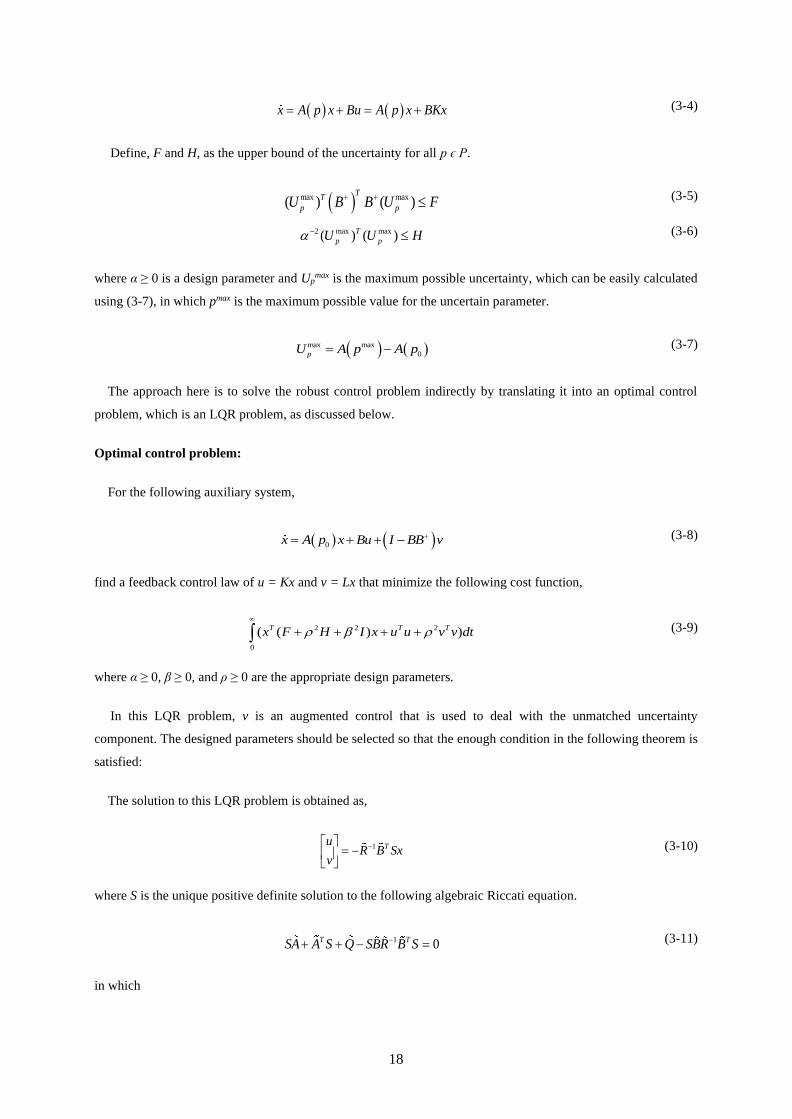
18

( ) ( )x A p x Bu A p x BKx= + = + (3-4)

Define, F and H, as the upper bound of the uncertainty for all p ϵ P.

( )max max( ) ( )T

T

p pU B B U F+ + (3-5)

2 max max( ) ( )T

p pU U H − (3-6)

where α ≥ 0 is a design parameter and Upmax is the maximum possible uncertainty, which can be easily calculated

using (3-7), in which pmax is the maximum possible value for the uncertain parameter.

( ) ( )max max

0pU A p A p= − (3-7)

The approach here is to solve the robust control problem indirectly by translating it into an optimal control

problem, which is an LQR problem, as discussed below.

Optimal control problem:

For the following auxiliary system,

( ) ( )0x A p x Bu I BB v+= + + − (3-8)

find a feedback control law of u = Kx and v = Lx that minimize the following cost function,

2 2 2

0

( ( ) )T T Tx F H I x u u v v dt

+ + + + (3-9)

where α ≥ 0, β ≥ 0, and ρ ≥ 0 are the appropriate design parameters.

In this LQR problem, v is an augmented control that is used to deal with the unmatched uncertainty

component. The designed parameters should be selected so that the enough condition in the following theorem is

satisfied:

The solution to this LQR problem is obtained as,

1 Tu

R B Sxv

− = −

(3-10)

where S is the unique positive definite solution to the following algebraic Riccati equation.

1 0T TSA A S Q SBR B S−+ + − = (3-11)

in which

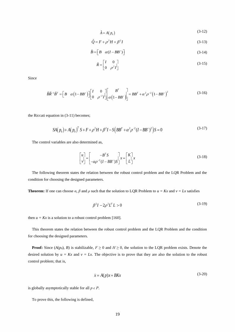
19

( )0A A p= (3-12)

2 2Q F H I = + + (3-13)

( )B B I BB + = − (3-14)

2

0

0

IR

I

=

(3-15)

Since

( )( )

( )2

1 2 2

2

01 1

0 1

T

T TBI

BR B B BB BB BBI BB

− + − +

− +

= − = + − −

(3-16)

the Riccati equation in (3-11) becomes;

( ) ( ) ( )2 2 2 2 2

0 0 ( ) 0T TSA p A p S F H I S BB I BB S − ++ + + + − + − =

(3-17)

The control variables are also determined as,

2 ( )

Tu KB Sx x

v LI BB S − +

− = =

− −

(3-18)

The following theorem states the relation between the robust control problem and the LQR Problem and the

condition for choosing the designed parameters.

Theorem: If one can choose α, β and ρ such that the solution to LQR Problem to u = Kx and v = Lx satisfies

2 22 0TI L L − (3-19)

then u = Kx is a solution to a robust control problem [160].

This theorem states the relation between the robust control problem and the LQR Problem and the condition

for choosing the designed parameters.

Proof: Since (A(p0), B) is stabilizable, F ≥ 0 and H ≥ 0, the solution to the LQR problem exists. Denote the

desired solution by u = Kx and v = Lx. The objective is to prove that they are also the solution to the robust

control problem; that is,

( )x A p x BKx= + (3-20)

is globally asymptotically stable for all p ϵ P.

To prove this, the following is defined,

20

2 2 2

0

min ( ( ) )m

T T T

u RV x F H I x u u v v dt

= + + + + (3-21)

to be the minimum cost of the optimal control of the auxiliary system from an initial state x0 to the origin.

It should be shown that V is a Lyapunov function for the system given in (3-20). By definition, V must satisfy

the Hamilton-Jacobi-Bellman equation which reduces to

( ) ( ) ( )( )2 2 2

0,

min{ } 0T T T T

xu v

x F H I x u u v v V A p x Bu I BB v ++ + + + + + + − = (3-22)

Since u = Kx and v = Lx are the optimal control, the follow identities must be satisfied;

( ) ( )( )2 2 2

0 0T T T T T T T T

xx Fx x Hx x x x K Kx x L Lx V A p x BKx I BB Lx ++ + + + + + + − = (3-23)

2 0T T T

xx K V B+ = (3-24)

( )22 0T T T

xx L V I BB ++ − = (3-25)

By considering (3-23) minus (3-24), it can be inferred that V(x) is a Lyapunov function for (3-20). It is

obvious that

0 0T

xV x (3-26)

0 0T

xV x= = (3-27)

to show dV/dt < 0 for all x ≠ 0, from (3-21), it yields,

( ) ( )( )T T

x xV x V x V A p x BKx= = + (3-28)

( ) ( ) ( )( ) ( ) ( )( )0

T T

x x pV x V A p x BKx I BB Lx V U x I BB Lx + += + + − + − − (3-29)

( ) ( ) ( )( ) ( ) ( )0

T T T

x x p xV x V A p x BKx I BB Lx V U x V I BB Lx+ += + + − + − − (3-30)

( ) ( ) ( )( ) ( ) ( )( ) ( )0

T T T T

x x p x p xV x V A p x BKx I BB Lx V BB U x V I BB U x V I BB Lx + + + += + + − + + − − − (3-31)

from (3-23), the first term of (3-31) can be expressed as (3-32),

( ) ( )( ) ( )2 2 2

0

T T T T T T

xV A p x BKx I BB Lx x F H I x x K Kx x L Lx ++ + − = − + + − − (3-32)

and from (3-24), the second term of (3-31) can be expressed as (3-33),

( ) ( )2T T T

x p pV BB U x x K B U x+ += − (3-33)

and from (3-25), the third and fourth terms of (3-31) can be expressed as (3-34) and (3-35),

21

( ) 22T T T

xV I BB Lx x L Lx +− = − (3-34)

( )( ) ( )1 22T T T

x p pV I BB U x x L U x + −− = − (3-35)

substituting (3-32) - (3-35) in (3-31), it yields,

( ) ( ) ( )( ) ( ) ( )( )

( )

0

T T T

x x p x p

T

x

V x V A p x BKx I BB Lx V BB U x V I BB U x

V I BB Lx

+ + +

+

= + + − + + −

− − (3-36)

( ) ( ) ( )

( )

2 2 2 2

1 2

2 2

2

T T T T T T T T T

p

T T

p

V x x F H I x x K Kx x L Lx x K B U x x L Lx

x L U x

+

−

= − + + − − − +

− (3-37)

the second and fourth terms of (3-37) can be expressed as (3-38),

( ) ( ) ( ) ( ) ( )

( ) ( )

2T T

T T T T T T

p p p p p

TT T

p p

x K Kx x K B U x x K B U K B U x x B U B U

x B U B U x x Fx

+ + + + +

+ +

− − = − − − +

(3-38)

considering (3-5) and (3-39) yields;

( ) ( ) ( ) ( ) ( ) ( )T T T

T T T T

p p p p p px K B U K B U x x B U B U x B U B U x x Fx+ + + + + +− − − + (3-39)

considering (3-6) and the fifth term of (3-37)

( )1 2 2 2 2 2 22 T T T T T T T T T

p P Px L U x x L Lx x U U x x L Lx x Hx − −− + + (3-40)

substituting (3-39) and (3-40) in (3-37), it yields

( ) ( )

( ) ( )

( )

( )

2 2 2

2 1 2

2 2 2 2 2 2

2 2

2 2 2

2

2

T T T T T

T T T T T T

p p

T T T T T T T T T

T T

V x x F H I x x K Kx x L Lx

x K B U x x L Lx x L U x

x F H I x x L Lx x Fx x L Lx x Hx x L Lx

x I L L x

+ −

= − + + − −

− + −

− + + − + + − +

= −

(3-41)

Consequently, if β2I−2ρ2LTL > 0 condition is satisfied, then, dV/dt will be negative for all x ≠ 0, and the

optimality necessary condition is met.

Accordingly, by the Lyapunov stability theorem, the system given in (3-4) is stable for all p ϵ P. In other

words, u = Kx is a solution to the Robust Control Problem.

Although the proposed optimal control approach for robust control of the excitation system has assumed no

nonlinear characteristic, however, the same approach can be applied to nonlinear systems. The nonlinear optimal

controls are usually obtained by solving the Hamilton–Jacobi–Bellman equations. Sometimes it is quite

complicated and time-consuming to obtain the solutions. An alternative approach to solve the nonlinear optimal

control problem is the State-Dependent Riccati Equation. This approach factorizes nonlinear state equations as

22

linear-like state equations having state-dependent coefficients, so the equations are written like the formulation

of the LQR. Thus, LQR optimal control can be solved to obtain optimal solutions [160].

3.4 Design of an Optimal Robust Excitation System

In this section, the aim is to implement the optimal robust control design strategy developed in the previous

section on the IEEE ST1A excitation system controller. In the IEEE ST1A excitation system, the excitation

power is provided through a transformer from the terminals of the generator (or the auxiliary bus) and is

regulated by a controlled rectifier; so, the maximum possible excitation voltage is directly related to the

generator terminal voltage [161]. In this model, alternative protection systems such as under excitation and

overexcitation limiters are ignored. Figure 3-1 shows the IEEE type ST1A simplified model.

1

1

C

B

sT

sT

+

+ 1

A

A

K

sT+∑∑

1

F

F

sK

sT+

1

R

R

K

sT+

tV cV

RefV

eV

2V

1VAV

FDE_

_

Figure 3-1: IEEE Type ST1A simplified excitation system model.

From Figure 3-1, the state space representation of the IEEE ST1A excitation system can be formulated as

x Ax Bu= + (3-42)

where the output is given by

y Cx Du= + (3-43)

in which y is the output vector, C is the output matrix and D is the feedforward matrix.

By considering the state vector, x = [V1 V2 Vc VA]T, the input vector, u = [Vt VRef ]T and the output vector, y =

[EFD], the state space representation matrices are expressed as,

1 1 1

10

10 0 0

10 0

C A F C F C C F

B B A F B B F B B R B A F

A F F

A F F A F

R

A

A A

T K K T K T T K

T T T T T T T T T T T T T

K K K

T T T T TA

T

K

T T

− − − − + +

−− = − −

(3-44)

23

10 0

10 0 0

C

B R RT

B

T

T T TB

T

− =

(3-45)

0 0 0 1C = (3-46)

0 0D = (3-47)

Considering the state space representation of the IEEE ST1A excitation system model, the proposed optimal

robust control design strategy given in section 3.3 can be applied. The reported nominal values in Table 3-1 for

the parameters of the IEEE ST1A excitation system model is adapted from [161].

Table 3-1: IEEE ST1A excitation system model parameters

Parameter Parameter description Nominal value

TR Regulator input filter time constant 0.02

KR Regulator filter gain 1

TC Regulator time constant 1

TB Regulator time constant 5

KA Amplifier gain 210

TA Amplifier time constant 0.02

KF stabilizer gain 0.02

TF stabilizer time constant 0.7

In the IEEE ST1A excitation system controller, the parameter directly impacts the closed-loop feedback

controller as the amplification gain. It is expected that KA significantly impact the dynamic behaviour of the

IEEE ST1A excitation system controller. To assess the impact of KA on the performance of the excitation system

controller, six different values of KA are selected; and for each of these values, the real parts of the eigenvalues

are evaluated. To demonstrate this, the value of KA can vary between ±20% of their nominal values. Table 3-2

has presented the results of eigenvalue analysis for each value of KA in the IEEE ST1A excitation system model.

Table 3-2: The real part of the eigenvalues for different values of KA without the optimal robust modification

Eigenvalue 1 2 3 4

KA - 0.2KA -1.68×103 -48.57 -1.42 -50

KA - 0.1KA -1.89×103 -48.57 -1.42 -50

KA - 0.05KA -1.99×103 -48.57 -1.42 -50

KA -2.10×103 -48.57 -1.42 -50

KA + 0.05KA -2.20×103 -48.57 -1.42 -50

KA + 0.1KA -2.31×103 -48.57 -1.42 -50

KA + 0.2KA -2.52×103 -48.57 -1.42 -50

24

Referring to Table 3-2, it can be concluded that as the value of KA is varied, the position of the real part of

eigenvalue 1 changes noticeably while the positions of the real parts of the other eigenvalues (2, 3, and 4) are

unchanged. This confirms that the uncertainty in the KA parameter has a significant influence on the dynamic

characteristic of the excitation system. By substituting the nominal values of the parameters from Table 3-1 in

(3-46), the system input matrix is given by,

10 0 50 0

0.2 0 0 0

TB−

=

(3-48)

The variable, Up, representing the uncertainty matrix, can be evaluated using (3-2), where KA represents the

uncertain parameter and, KA0 represents the nominal value of the uncertain parameter, KA. In Table 3-1, the value

of KA0 is reported to be 210, so, the uncertainty in parameter KA is given by

0

2100.2 10.2 0 0 0

1.43 300 0 0 0( ) ( )

0 0 0 0

50 10500 0 0 0

A

A

p A A

A

K

KU A K A K

K

−

− = − =

−

(3-49)

The uncertainty can be divided into the matched and the unmatched components using the Moore-Penrose

pseudo-inverse of B denoted by B+ as follows:

198.67 10 0 0.02 0

5 0 1 0B

−

+ −

=

(3-50)

Using (3-3), the corresponding matched and unmatched components are computed as,

16 14

2100.2 10.2 0 0 0

0 0 0 0

4.4 10 9.11 10 0 0 0

0 0 0 0

A

Matched

p

A

K

UK− −

− = −

(3-51)

13 14

14 16

2.33 10 1.13 10 0 0 0

1.43 300 0 0 0

9.11 10 4.42 10 0 0 0

50 10500 0 0 0

A

Unmatched A

p

A

A

K

KU

K

K

− −

− −

−

− = −

−

(3-52)

Now, the upper bound of the uncertainty for all p ϵ P should be calculated. To do so, the maximum

uncertainty, Upmax by considering KA

max = 310 is obtained as,

max

1000 0 0 0

142.9 0 0 0

0 0 0 0

5000 0 0 0

pU

− =

(3-53)

25

Finally, from (3-5) and (3-6) the value of F and H are determined, by considering α = 1, as below.

72.5 10 0 0 0

0 0 0 0

0 0 0 0

0 0 0 0

F

=

(3-54)

72.602 10 0 0 0

0 0 0 0

0 0 0 0

0 0 0 0

H

=

(3-55)

The algebraic Riccati equation in (3-11) can be formed by considering the design parameters as β = 10 and ρ

= 1. The solution to the algebraic Riccati equation denoted by S is given as follows,

823.09 0.84 26.68 1.5

0.84 8.68 0.17 0.216

26.68 0.17 5.47 0.28

1.5 0.216 0.28 0.99

S

− − − −

= −

−

(3-56)

Using S, the closed-loop controller, and the augmented controller are computed using (3-18) as below.

6896.9 0.29 6.86 1.06

164.6 0.17 5.33 0.3K

− =

− − − (3-57)

and

14 16 15 16

14 17 15 17

9.2 10 1 10 3.2 10 1.8 10

0.84 8.68 0.17 0.216

4.5 10 4.7 10 1.4 10 8.3 10

1.5 0.216 0.28 0.99

L

− − − −

− − − −

− −

− − − = −

−

(3-58)

and then the new system matrix, Anew, is expressed as,

4

5

7.1 10 3.05 77.31 10.36

300 1.42 0 1.42

3.4 10 14.47 392.9 52.97

10500 0 0 50

newA A BK

− − −

− − = + = −

−

(3-59)

To evaluate the robustness of the developed strategy, the eigenvalue analysis is performed. Using the same six

different values of KA in Table 3-2 (±20% variation in KA from its nominal value), the positions of the real parts

of the system eigenvalues for different KA values are evaluated. Table 3-3 shows the results of eigenvalue

analysis for the IEEE ST1A excitation system model with the proposed optimal robust controller parameters.

Table 3-3 reveals that as KA is varied, the changes in the positions of the real parts of all eigenvalues are

unchanged. This confirms that the designed robust IEEE ST1A excitation controller model is robust for ±20%

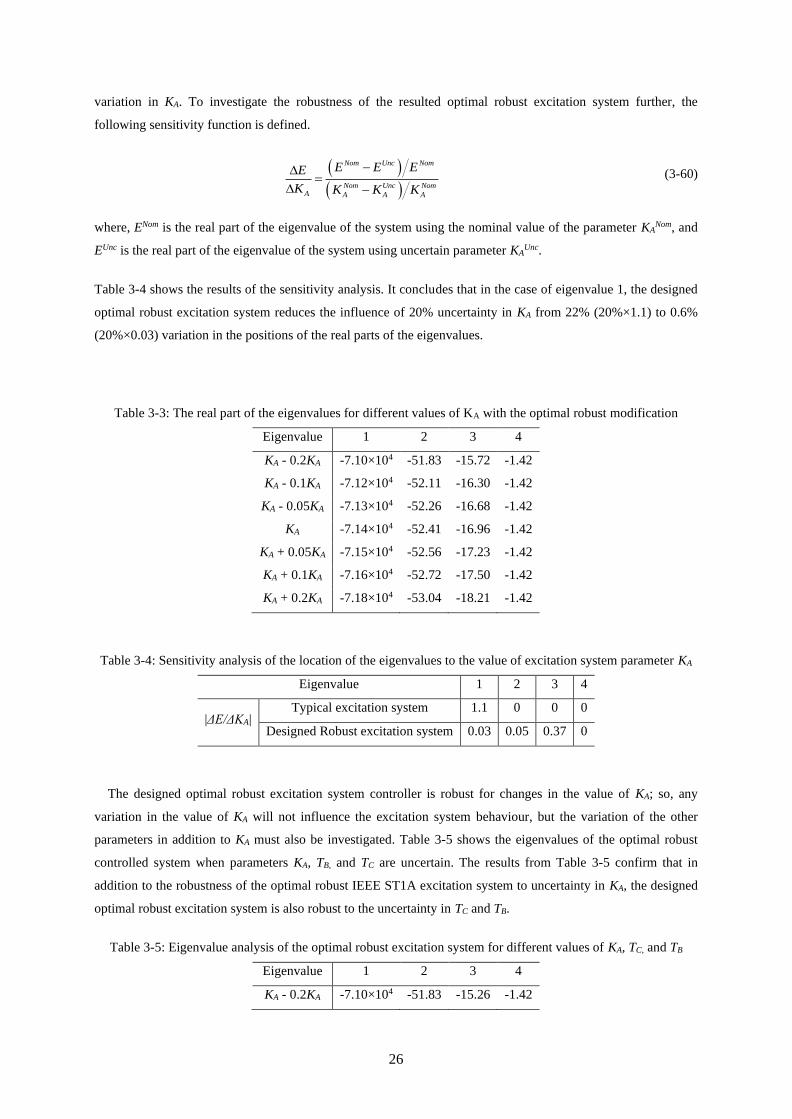
26

variation in KA. To investigate the robustness of the resulted optimal robust excitation system further, the

following sensitivity function is defined.

( )( )

Nom Unc Nom

Nom Unc NomA A A A

E E EE

K K K K

−=

− (3-60)

where, ENom is the real part of the eigenvalue of the system using the nominal value of the parameter KANom, and

EUnc is the real part of the eigenvalue of the system using uncertain parameter KAUnc.

Table 3-4 shows the results of the sensitivity analysis. It concludes that in the case of eigenvalue 1, the designed

optimal robust excitation system reduces the influence of 20% uncertainty in KA from 22% (20%×1.1) to 0.6%

(20%×0.03) variation in the positions of the real parts of the eigenvalues.

Table 3-3: The real part of the eigenvalues for different values of KA with the optimal robust modification

Eigenvalue 1 2 3 4

KA - 0.2KA -7.10×104 -51.83 -15.72 -1.42

KA - 0.1KA -7.12×104 -52.11 -16.30 -1.42

KA - 0.05KA -7.13×104 -52.26 -16.68 -1.42

KA -7.14×104 -52.41 -16.96 -1.42

KA + 0.05KA -7.15×104 -52.56 -17.23 -1.42

KA + 0.1KA -7.16×104 -52.72 -17.50 -1.42

KA + 0.2KA -7.18×104 -53.04 -18.21 -1.42

Table 3-4: Sensitivity analysis of the location of the eigenvalues to the value of excitation system parameter KA

Eigenvalue 1 2 3 4

|ΔE/ΔKA| Typical excitation system 1.1 0 0 0

Designed Robust excitation system 0.03 0.05 0.37 0

The designed optimal robust excitation system controller is robust for changes in the value of KA; so, any

variation in the value of KA will not influence the excitation system behaviour, but the variation of the other

parameters in addition to KA must also be investigated. Table 3-5 shows the eigenvalues of the optimal robust

controlled system when parameters KA, TB, and TC are uncertain. The results from Table 3-5 confirm that in

addition to the robustness of the optimal robust IEEE ST1A excitation system to uncertainty in KA, the designed

optimal robust excitation system is also robust to the uncertainty in TC and TB.

Table 3-5: Eigenvalue analysis of the optimal robust excitation system for different values of KA, TC, and TB

Eigenvalue 1 2 3 4

KA - 0.2KA -7.10×104 -51.83 -15.26 -1.42

27

TB - 0.2TB

TC - 0.2TC

KA - 0.1KA

TB - 0.1TB

TC - 0.1TC

-7.12×104 -52.11 -16.11 -1.42

KA - 0.05KA

TB - 0.05TB

TC - 0.05TC

-7.13×104 -52.26 -16.53 -1.42

KA + 0.05KA

TB + 0.05TB

TC + 0.05TC

-7.15×104 -52.56 -17.39 -1.42

KA + 0.1 KA

TB + 0.1TB

TC + 0.1TC

-7.16×104 -52.72 -17.81 -1.42

KA + 0.2KA

TB + 0.2TB

TC + 0.2TC

-7.18×104 -53.04 -18.66 -1.42

3.5 Case Study

In this study, the uncertainty in the values of the most critical parameters of the IEEE ST1A excitation system

is considered. The uncertainty study is implemented by considering ±10% and ±20% changes in the values of

selected parameters from the nominal values given in Table 3-1. The time-domain dynamic stability simulation

has been performed using DIgSILENT PowerFactory, using the IEEE ST1A excitation system controller for all

generators. The first case is the transient stability analysis of a single machine system given in [162], where there

is uncertainty in the value of KA. In this case, the studies are performed for the conditions where the test system

is under high stress (Peak load demand). Figure 3-2 shows the single line diagram of the single-machine test

system.

S

External

GridM

2

1

3

4

5 Load

Motor

Generator

L1-3

L1-3b

TR2-3

TR3-4

TRLoad

L3-5

Figure 3-2: Single line diagram of the single-machine test system.

The influences of the uncertainties of the parameters in the IEEE ST1A excitation system parameters on the

voltage profiles of Bus 5 is illustrated in Figures 3-3 and 3-4 for both the unmodified and the modified IEEE

ST1A excitation system models, respectively.

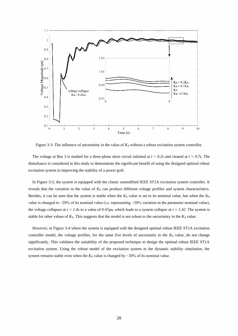
28

Figure 3-3: The influence of uncertainty in the value of KA without a robust excitation system controller.

The voltage at Bus 3 is studied for a three-phase short circuit initiated at t = 0.2s and cleared at t = 0.7s. The

disturbance is considered in this study to demonstrate the significant benefit of using the designed optimal robust

excitation system in improving the stability of a power grid.

In Figure 3-3, the system is equipped with the classic unmodified IEEE ST1A excitation system controller. It

reveals that the variation in the value of KA can produce different voltage profiles and system characteristics.

Besides, it can be seen that the system is stable when the KA value is set to its nominal value, but when the KA

value is changed to −20% of its nominal value (i.e. representing −20% variation in the parameter nominal value),

the voltage collapses at t = 1.4s to a value of 0.47pu, which leads to a system collapse at t = 1.42. The system is

stable for other values of KA. This suggests that the model is not robust to the uncertainty in the KA value.

However, in Figure 3-4 where the system is equipped with the designed optimal robust IEEE ST1A excitation

controller model, the voltage profiles, for the same five levels of uncertainty in the KA value, do not change

significantly. This validates the suitability of the proposed technique to design the optimal robust IEEE ST1A

excitation system. Using the robust model of the excitation system in the dynamic stability simulation, the

system remains stable even when the KA value is changed by −20% of its nominal value.

29

Figure 3-4: The influence of uncertainty in the values of KA considering a robust excitation system controller.

Sensitivity studies have also been carried out to investigate the operation of the proposed controller when the

controller setpoints are varied [163]; in particular, the impact of varying the generator reference voltage (VRef)

from 0.9 to 0.95 and finally 1.0 is investigated. The impact of varying VRef on the voltage of bus 5 is shown in

Figure 3-5. Figure 3-5 shows that despite the significant changes in the values of the voltage at bus 5 after

varying VRef, the performance of the control system remains robust to uncertainties in the value of parameters

when KA is varied from −20% to +20% in the zoomed areas. Consequently, it can be concluded that the

robustness of the proposed optimal robust excitation system controller is not sensitive to variations in the value

of the generator reference voltage.

30

Figure 3-5: The voltage at bus 5 using the proposed robust excitation system for different generator reference

voltages, with the uncertainty in the values of KA.

The second case is the dynamic stability analysis of the IEEE 39-bus New England system, presented in

Figure 3-6 and detailed in [98], where there are uncertainties in the values of KA, TB, and TC.

Figure 3-6: Single line diagram of the IEEE 39-buses New England test system.

31

In this case, it is assumed that all generators are equipped with the IEEE ST1A excitation system

controller, where there are uncertainties in the parameter values of KA, TB, and TC. A three-phase solid

short circuit is considered at Bus 2 at t = 0.2s which is cleared at t = 1.4s. The result for the voltage at

Bus 25 in the New England system after the disturbance is presented in Figures 3-7 and 3-8 for the

system without and with the optimal robust IEEE ST1A excitation system controller designed using

the proposed framework. Figure 3-7 shows that when the KA, TB, and TC values are changed by −20%

of their nominal values when the classical excitation controller model is used, the system collapses at t

= 1.79s, while it is stable for other values of KA, TB, and TC. This demonstrates that the ST1A

excitation controller is not robust against the uncertainties of KA, TB, and TC.

Figure 3-7: The influences of uncertainty in the values of KA, TB, and TC without a robust excitation system

controller at high loading level.

Figure 3-8 represents that when the system is equipped with the optimal robust IEEE ST1A

excitation controller, the voltage profiles for all five levels do not change significantly, and even when

the values of KA, TB and TC are set to −20% of their nominal values, the system remains stable.

32

Figure 3-8: The influences of uncertainty in the values of KA, TB, and TC considering a robust excitation system

controller at high loading level.

The results from Figures 3-7 and 3-8 have been summarised in Table 3-5.

Table 3-6: Comparison between the excitation control system performance with and without the robust

improvement for IEEE 39 bus network

Parameter Variation

KA, TB, TC

Maximum voltage deviation

Without robust excitation system With robust excitation system

+20% 1.6% 0.2%

+10% 1.1% 0.1%

0% 0 0

-10% -1.2% 0.1%

-20% Voltage collapse 0.2%

In this study, the load demand is high and the system is heavily loaded. The sensitivity of the

proposed optimal robust controller to the variation in the load demand of the power system is also

investigated for the case of the low and medium load demand conditions of the grid. Table 3-7

presents a summary of the loading levels.

Table 3-7: Different loading conditions considered in the second case study

Loading Level New England Test system

Load (MW) Load (MVAr)

High 6822 1525

33

Medium 6139.8 1372.5

Low 5457 1220

Figure 3-9 shows that the robustness of the proposed optimal robust excitation system controller is

maintained for different loading levels of the power grid. The optimal robust approach introduced in

this study can be easily implemented for any type of excitation system controllers to improve its

robustness when the data of the excitation system controllers contains unavoidable uncertainties in its

parameters.

Figure 3-9: The influences of uncertainty in the values of KA, TB, and TC considering robust excitation system

controller – A comparison for high, medium, and low loading levels.

3.6 Summary

This chapter has presented a new optimal robust IEEE ST1A excitation system controller that is

robust to the uncertainty in one or more of its parameters. Despite the complex mathematics behind the

method, it can be implemented simply and straightforwardly, even though uncertainties in the model

parameters exist. This optimal approach has transferred the robust controller problem to an optimal

control problem while it has preserved the robustness of the excitation system. The influences of

uncertainty in the values of KA, with and without the design of the robust excitation system controller

have been investigated for a single machine test system.

34

The simulation results from the dynamic stability simulation have demonstrated that the designed

robust excitation system controller is capable of being robust to uncertainty in the parameters of an

excitation system controller. For the IEEE 39 bus system, simulation results show that when the KA, TB

and TC values of the IEEE ST1A excitation system controller are changed to −20% of their nominal

values, the system becomes unstable although the system was stable when other values (within the

upper and lower limit) were used. However, when the designed optimal robust IEEE ST1A excitation

system controller has been applied, the system has become robust to the uncertainties in the

parameters of the excitation system controller. Irrespective of the values of the parameters within the

boundary of the uncertainties, using the proposed robust controller the power system will not have any

variation in its stability.

35

Chapter 4 Long-term Voltage Stability Improvement

4.1 Foreword

There is always a time gap between a disturbance in the power system and voltage collapse, this time is very

critical to the planners to implement reliable and economical countermeasures and resolve voltage related

abnormalities. The proposed overexcitation limiter (OEL) extends the time gap between a disturbance in the

power system and voltage collapse and allows the synchronous machine to participate in supplying the reactive

power deficiency in the grid, which is critical in reactive power mismatch related emergency condition

management.

Voltage stability requires the continuing control of the total system’s supply of reactive power during an

emergency. The supply of reactive power, however, can be curtailed by the action of rotor over-current

protection or OEL in reducing the rotating unit reactive power output. Practical heat run tests show that the

timing of the activation of the OEL can be very conservative, resulting in earlier than necessary operation and

system voltage collapse. Significant benefit can be achieved if the timing of the OEL activation can be delayed

while ensuring enough margin is provided to avoid harming the rotor of the synchronous generator from

overheating. This chapter proposes a new thermal-based method to determine the timing of the OEL activation

that is based on the thermal capacity of the rotor as the main indicator for limiting the over-rated excitation level

of the synchronous generator. The proposed thermal-based method is validated using extensive simulations of a

single-machine and the Nordic power system. Simulation studies show that the system voltage collapse can be

delayed significantly by delaying the OEL activation without compromising the thermal capacity of the rotor if

the proposed OEL setting is used.

4.2 Background

During a catastrophic situation, where the line or generator outages are more than the planned n-1

contingencies, the synchronous generator can provide additional required reactive power by increasing their

excitation level for a limited period. To protect the rotor winding from overheating due to high rotor excitation

current while simultaneously allowing maximum field forcing for power system voltage stability purposes, the

allowed over-excitation period is determined by the OEL. The OEL may reduce the excitation level by

instantaneously lowering the reference set point, by ramping or stepping down the reference set point, or by

transferring control from the AVR to a lower manually controlled field voltage set point [161]. The timing of this

protection is very conservative, without considering the initial and maximum safe rotor temperature. The OEL

should be capable of limiting the excitation current before the field over-current protection either place the AVR

into the manual mode or trips the exciter to protect the field winding from overheating. Moreover, the field over-

current protection should be coordinated with the OEL settings to allow the exciter to effectively provide its full

VAr capability during continuous or transient conditions.

According to the stability definition of the IEEE/CIGRE task force [17], voltage stability refers to the ability

of a power system to maintain steady voltages at all buses in the system after being subjected to a disturbance

36

from a given initial operating condition. This event is characterized by a slow variation of the voltage

magnitudes followed by a rapid sharp disruptive phase resulting in voltage collapse [2]. In the first phase of

voltage stability with the outages of several transmission lines or generating units beyond planning criteria, the

reactive power loss increases rapidly in the remaining transmission lines. The generating units near the most

affected region increase the excitation level to produce more reactive power and balance the supply and demand

of reactive power [164], resulting in a stable operating condition during the first phase of voltage stability.

However, to protect the rotor from overheating, successive OEL operations progressively reduce the reactive

power support causing the imbalance between the supply and demand of reactive power leading to the second

fast phase of voltage instability. Much work has been done on ensuring that the load shedding is carried out

before the onset of the second phase of voltage instability [84], [165].

However, by investigating the initial rotor temperature and thermal capacity, the OEL protection setting is

very conservative; in some cases, the OEL operates even when more than 90% of the rotor thermal capacity is

still available to be used [164]. The current OEL systems do not take into consideration the temperature of the

rotor winding for rotor over current protection. Consequently, the initial temperature of the rotor (overheated due

to a previous disturbance), cooling system performance, and environmental factors are not considered. As all

these so-called key factors are neglected in the rotor overcurrent protection, significant risk is involved in using

the rotor thermal capability. As a result, traditionally, the OEL systems are tuned in a very conservative manner.

Delaying the OEL operation can delay the onset of the second phase of instability resulting in having more

time to consider the best countermeasures to be carried out and such delay can result in better management of

voltage instability.

4.3 Automatic Voltage Regulators and Over-Excitation Limiter

Automatic Voltage Regulators (AVRs) can provide a rapid response of the synchronous generator reactive

power output to maintain the pre-set voltage. During the normal operating condition, the AVR can vary the

voltage between ±5% to ±10% from its nominal condition [17], and during an emergency condition, the AVR

can produce higher than rated excitation current, typically up to two times of the rated value [161]. Although the

rotor winding is designed for a continuous level of current, higher than rated current can be sustained by the

rotor for a limited time; this limited time is usually determined by the OEL in the AVR control system.

4.3.1 Excitation System Perspective

Different strategies have been considered in implementing the OEL system in the AVR control system [161],

[80], [165]. In this study, the OEL is used to reduce the excitation level by adding an extra auxiliary input signal

for the AVR system that simulates an extra error signal in the voltage regulation process as shown in Figure 4-1

where VT is generator terminal voltage, Vref is the reference voltage, Vpss is the signal from power system

stabilizer (PSS), VOEL is the signal from OEL, VRmax and VRmin are the maximum and minimum voltage regulator

outputs.

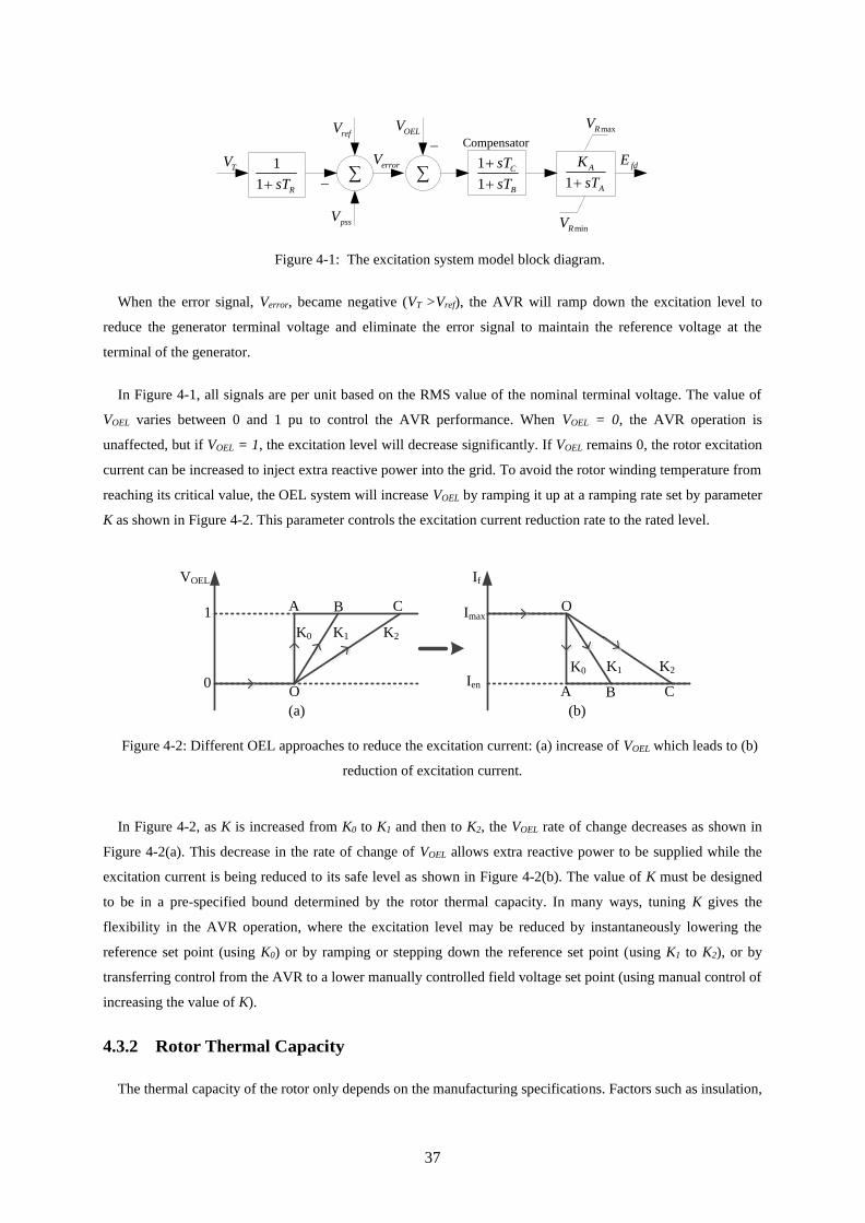
37

∑ 1

1 RsT+

1

1

C

B

sT

sT

+

+ 1

A

A

K

sT+

TV

refV

fdE

−

minRV

maxRV

Compensator

∑

OELV

errorV

pssV

−

Figure 4-1: The excitation system model block diagram.

When the error signal, Verror, became negative (VT >Vref), the AVR will ramp down the excitation level to

reduce the generator terminal voltage and eliminate the error signal to maintain the reference voltage at the

terminal of the generator.

In Figure 4-1, all signals are per unit based on the RMS value of the nominal terminal voltage. The value of

VOEL varies between 0 and 1 pu to control the AVR performance. When VOEL = 0, the AVR operation is

unaffected, but if VOEL = 1, the excitation level will decrease significantly. If VOEL remains 0, the rotor excitation

current can be increased to inject extra reactive power into the grid. To avoid the rotor winding temperature from

reaching its critical value, the OEL system will increase VOEL by ramping it up at a ramping rate set by parameter

K as shown in Figure 4-2. This parameter controls the excitation current reduction rate to the rated level.

A

VOEL

O

B C

0

1

K1 K2

O

If

A B CIen

Imax

K1 K2K0

K0

(a) (b)

Figure 4-2: Different OEL approaches to reduce the excitation current: (a) increase of VOEL which leads to (b)

reduction of excitation current.

In Figure 4-2, as K is increased from K0 to K1 and then to K2, the VOEL rate of change decreases as shown in

Figure 4-2(a). This decrease in the rate of change of VOEL allows extra reactive power to be supplied while the

excitation current is being reduced to its safe level as shown in Figure 4-2(b). The value of K must be designed

to be in a pre-specified bound determined by the rotor thermal capacity. In many ways, tuning K gives the

flexibility in the AVR operation, where the excitation level may be reduced by instantaneously lowering the

reference set point (using K0) or by ramping or stepping down the reference set point (using K1 to K2), or by

transferring control from the AVR to a lower manually controlled field voltage set point (using manual control of

increasing the value of K).

4.3.2 Rotor Thermal Capacity

The thermal capacity of the rotor only depends on the manufacturing specifications. Factors such as insulation,

38

cooling system, and the materials used in building the rotor, directly impact the thermal capability of the rotor in

a generating unit. After the manufacturing and installation of the unit, the rotor thermal capability is likely to

remain constant unless the environmental conditions change significantly. The OEL system is used to avoid the

rotor thermal capability to be exhausted. An ideal OEL system is to monitor the available rotor thermal capacity

and reduce the excitation as the thermal capability is close to being exhausted. To reduce the risk of loss of life, a

safety margin is normally considered in the operation of the OEL in not using the whole rotor thermal capability.

This safety margin should be determined by balancing between the risk of loss of life and a pool of fast-acting

reactive power supply.

The available rotor thermal capacity depends on the rotor windings temperature; however, measuring the

temperature directly is not a practical option, because, the temperature snapshot of the machine elements is

usually only available every 30 seconds [165]. Consequently, different methods to measure the temperature were

reported; some use the rotor current and voltage [80], [81], while others use the dependency of the rotor winding

resistance to its temperature to calculate the temperature [165], [166].

Generally, for rotor over-heating protection a curve is used indicating the time for OEL activation for each

over-excited level in an inverse time function; the higher the rotor current, the sooner the limiter is activated. The

rotor capacity curves extracted from [167] are shown in Figure 4-3.

Figure 4-3: Rotor windings short circuit current capacity.

Figure 4-3 shows that the curve from [167] allows for a longer activation time of the OEL compared to that

from the curve from the ANSI C50.13-1989 standard for the same elevated excitation current. The curves in

Figure 4-3 use an inverse current-time characteristic very similar to overcurrent protection systems without

considering the thermal characteristic of the rotor, the cooling system, and also the environmental factors. To

avoid the risk of damage to the machine rotor winding, these factors are normally not considered and a very low-

risk OEL setting is used. Taking a very low-risk approach has led to very conservative OEL system settings.

Additionally, using the excitation current as an indicator for OEL operation it will be difficult to know the

39

remaining thermal capacity of the rotor winding.

In this study, rather than current, the thermal energy will be used as the main indicator to determine the OEL

activation time.

4.3.3 Over-excitation Limiter

Different types of OEL systems are presented in the literature [82], [86], [161], [168]–[171]; however, all of

them are operated through the same sequence of (i) detecting the over-excitation for a specified period and then

(ii) reducing it into a safe level. The allowed over-excitation period may be fixed-time or inverse-time. The

fixed-time OEL system enables a timer when it detects an over-excitation situation and reduces the rotor current

to its rated value when the timer reaches a fixed predetermined value. For the case of inverse-time OEL system,

this predetermined value varies inversely with the excitation level as shown in Figure 4-3. Typically, the OEL

system uses a combination of the instantaneous and the inverse-time pickup characteristics and switches from an

instantaneous limiter with a setting of about 160% of rated excitation current to a timed-limiter with a setting of

about 105% of the rated excitation current [80], [172].

4.4 Thermal Based OEL

The proposed method uses the thermal energy of the rotor to determine the auxiliary signal VOEL for the AVR

in Figure 4-1 and the ramp rate K to determine the timing for the activation of OEL. This method can be easily

implemented on the AVR. Following the recommendation of ANSI C50.13, at least a 20% safety margin must

be provided.

The thermal energy of the rotor winding during the over-excitation period needs to be calculated and

monitored to ensure that the rotor overheating is safe. The cooling system capability, the initial temperature of

the rotor, and the heat transfer from the turbine need to be taken into consideration. To calculate the thermal

energy of the rotor winding, the law of conservation of energy for all the components which influence rotor

temperature can be calculated as in (4-1),

Copper Turbine Winding DissipationQ Q Q Q+ = + (4-1)

where QCopper is the heat energy due to the copper losses of the current passing through the rotor windings,

QTurbine is the indirect heat flow from the steam turbine that passes through the mechanical coupling between the

turbine and the generator, QWinding is the thermal energy of the rotor windings (the absorbed heat by winding) and

QDissipation is the combination of the energy due to heat dissipation through the pressurized hydrogen flowing in

the gap between stator and rotor, and, that due to the radiation and convection of the outer surface of the

generator to the surrounding air.

Equation (4-1) is based on the law of the conservation of the energy, so it is valid in both emergency

conditions given by (4-3) and normal operating conditions presented by (4-2). For simplicity, let’s consider E

and N as the superscripts for emergency and normal conditions of the system respectively.

40

N N N N


E E E E


For the next step let’s subtract (4-3) from (4-2) as given in (4-4),

E E N N E E N N

Copper Turbine Copper Turbine Winding Dissipation Winding DissipationQ Q Q Q Q Q Q Q+ − − = + − − (4-4)

In (4-4), QTurbine and QDissipation are equal as that in normal conditions; since, in an emergency condition, neither

cooling system capability has changed nor the airflow into the generator. Equation (4-4) can, therefore, be

simplified as given in (4-5),

E N E N

Copper Copper Windings WindingsQ Q Q Q− = − (4-5)

Equation (4-5) can be expressed as (4-6) where R, m and c are resistor, mass and the specific heat coefficient

of the rotor winding respectively, and TE, TN, IE and IN are the temperature increase and the current during the

emergency and the normal voltage condition.

2 2( ) ( )E N E N

R I I t mc T T− = − (4-6)

Equation (4-6) describes the relationship between the copper losses in the rotor winding of the generator with

the stored thermal energy inside the winding of the generator.

As the rotor current increases, the copper loss becomes greater than the dissipated heat. This excess energy

will then be absorbed in the rotor winding as thermal energy and will result in temperature rise. This extra

amount of heat energy can be calculated using the integral of the left-hand term of equation (4-6) as shown in (4-

7) where EAH is the Extra Absorbed Heat from t1 to t2 and, R is the rotor resistance in per unit.

2

1

2 2( )dt

E Nt

EAH R I I t= − (4-7)

The maximum amount of rotor current for the steady-state condition, Ien, is usually used in OEL to activate the

OEL operation. It is generally considered to be about 105% of rated field current. In (4-6), Ien can be used instead

of IN, and If, the measured rotor current, can be used instead of IE, to calculate EAH since it represents the

measured excitation current during emergency condition:

2

1

2 2( )dt

f ent

EAH R I I t= − (4-8)

The rotor cooling system is responsible for the dissipation of this EAH in addition to radiation and convection.

So, the main objective of our proposed method for the OEL setting is to monitor the value of EAH and prevent it

to go higher than the predetermined rotor thermal capacity, Ecap. The best method to calculate Ecap is to use the

right-hand term of (4-6) by replacing TE with Tmax as given in (4-9)

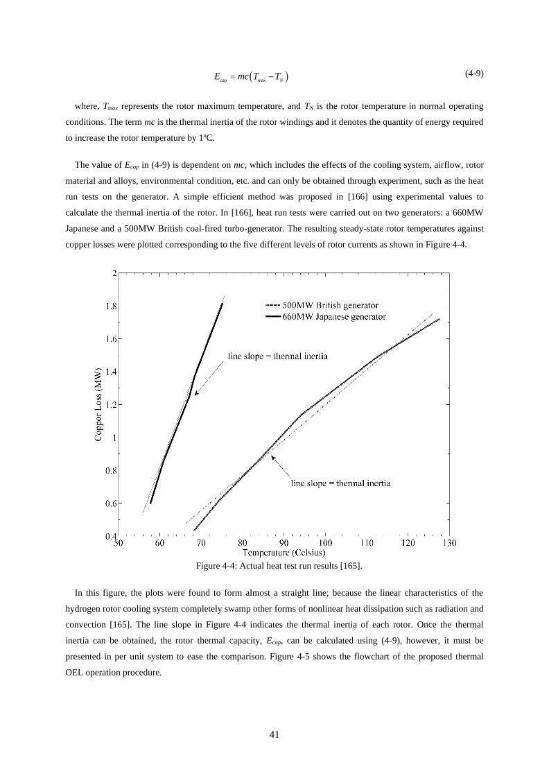
41

( )maxcap NE mc T T= − (4-9)

where, Tmax represents the rotor maximum temperature, and TN is the rotor temperature in normal operating

conditions. The term mc is the thermal inertia of the rotor windings and it denotes the quantity of energy required

to increase the rotor temperature by 1ºC.

The value of Ecap in (4-9) is dependent on mc, which includes the effects of the cooling system, airflow, rotor

material and alloys, environmental condition, etc. and can only be obtained through experiment, such as the heat

run tests on the generator. A simple efficient method was proposed in [166] using experimental values to

calculate the thermal inertia of the rotor. In [166], heat run tests were carried out on two generators: a 660MW

Japanese and a 500MW British coal-fired turbo-generator. The resulting steady-state rotor temperatures against

copper losses were plotted corresponding to the five different levels of rotor currents as shown in Figure 4-4.

Figure 4-4: Actual heat test run results [165].

In this figure, the plots were found to form almost a straight line; because the linear characteristics of the

hydrogen rotor cooling system completely swamp other forms of nonlinear heat dissipation such as radiation and

convection [165]. The line slope in Figure 4-4 indicates the thermal inertia of each rotor. Once the thermal

inertia can be obtained, the rotor thermal capacity, Ecap, can be calculated using (4-9), however, it must be

presented in per unit system to ease the comparison. Figure 4-5 shows the flowchart of the proposed thermal

OEL operation procedure.

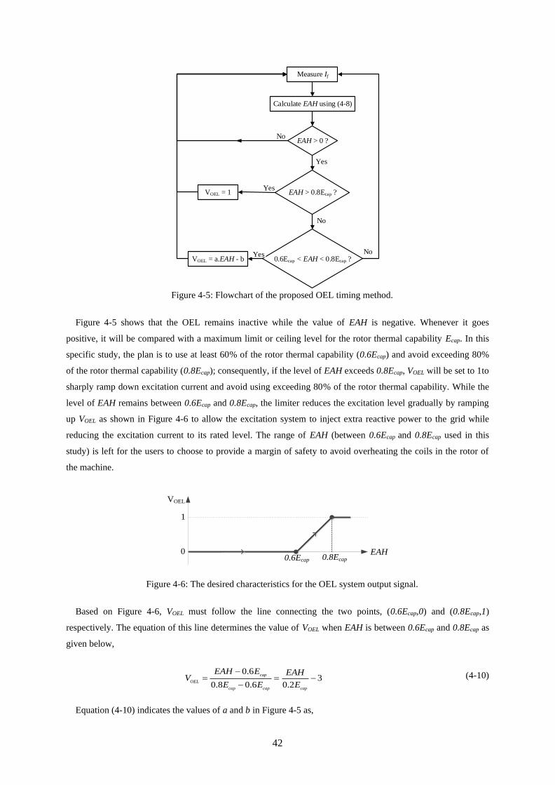
42

Measure If

Yes

No

Calculate EAH using (4-8)

EAH > 0 ?

EAH > 0.8Ecap ?VOEL = 1

0.6Ecap < EAH < 0.8Ecap ?VOEL = a.EAH - b

Yes

No

Yes No

Figure 4-5: Flowchart of the proposed OEL timing method.

Figure 4-5 shows that the OEL remains inactive while the value of EAH is negative. Whenever it goes

positive, it will be compared with a maximum limit or ceiling level for the rotor thermal capability Ecap. In this

specific study, the plan is to use at least 60% of the rotor thermal capability (0.6Ecap) and avoid exceeding 80%

of the rotor thermal capability (0.8Ecap); consequently, if the level of EAH exceeds 0.8Ecap, VOEL will be set to 1to

sharply ramp down excitation current and avoid using exceeding 80% of the rotor thermal capability. While the

level of EAH remains between 0.6Ecap and 0.8Ecap, the limiter reduces the excitation level gradually by ramping

up VOEL as shown in Figure 4-6 to allow the excitation system to inject extra reactive power to the grid while

reducing the excitation current to its rated level. The range of EAH (between 0.6Ecap and 0.8Ecap used in this

study) is left for the users to choose to provide a margin of safety to avoid overheating the coils in the rotor of

the machine.

VOEL

0

1

EAH0.6Ecap 0.8Ecap

Figure 4-6: The desired characteristics for the OEL system output signal.

Based on Figure 4-6, VOEL must follow the line connecting the two points, (0.6Ecap,0) and (0.8Ecap,1)

respectively. The equation of this line determines the value of VOEL when EAH is between 0.6Ecap and 0.8Ecap as

given below,

0.63

0.8 0.6 0.2

cap

OEL

cap cap cap

EAH E EAHV

E E E

−= = −

− (4-10)

Equation (4-10) indicates the values of a and b in Figure 4-5 as,

43

1

0.2

3

cap

aE

b

=

= −

(4-11)

Based on (4-10), the values of a and b are directly dependent on the value of Ecap and willingness of the

generating unit to use its rotor thermal capability. In this study, we maintained the rotor thermal capability usage

between 60% and 80%. Based on proper risk assessment, the generating using can use as much as 100% of the

rotor thermal capability in which will lead to different a and b coefficients.

The proposed OEL system model is presented in Figure 4-7. All parameters in this model are in per unit,

based on the rated value of the generator. In the diagram shown in Figure 4-7, y2 represents the surplus thermal

energy (EAH) that was absorbed by the rotor windings due to the over-excitation current. Whenever y2 is not

zero, the rotor faces over-excitation, but the OEL system remains disabled, which allows the machine to inject as

much reactive power as possible into the system until y2 reaches 0.6Ecap; when the OEL forces the AVR to ramp

down the excitation level to Ien.

Figure 4-7: The model of the OEL system with the proposed timing method.

Backup protection is also considered for the safety of the rotor that pushes the AVR to clamp the excitation

current to Ien instantly. This backup protection will get activated when y2 reaches 0.8Ecap and ensure the safety of

the rotor in case of any failure in the ramping down procedure.

4.5 The Proposed OEL Model Evaluation

To evaluate the proposed method for determining the OEL setting and to compare its performance with that of

the conventional OEL systems, a single-machine test system is considered as presented in Figure 4-8.

2

fI

2enI

−1

s1

y1

0y

10y 0

OELV

1

0

0y

20.8 capy E

20.8 capy E

20.6 capy E

0

20.6 capy E

rotR

1 0.2 capE −

3

2y

0

1

44

S

External

GridM

2

1

3

4

5 Load

Load (Motor)

Generator

L1-3

L1-3b

TR2-3

TR3-4

TRLoad

L3-5

Figure 4-8: Single line diagram of the single-machine test system.

The test system in Figure 4-8 is adapted from [162] and its generator is equipped with the proposed thermal-

based OEL system and a conventional OEL system introduced by IEEE in [161]. The thermal parameters of the

generator are adapted from the available test heat run data from a 660MW Japanese unit [166] with thermal

inertia of 10MJ/ºC, and a 500MW British generator unit [165] with thermal inertia of 3MJ/ºC. The simulations

are performed using DIgSILENT PowerFactory. The nominal operating range of the rotor temperature of these

generators was found to be between 65ºC and 75ºC while the rotor temperature limit lies between 130ºC and

140ºC [165]. Considering 65ºC increase in rotor temperature for the Japanese generator unit from its nominal

setpoint, Ecap is calculated using (4-9) as given below,

( )( )10 65 650cap

E MJ C C MJ= = (4-12)

Ebase is calculated using (4-13).

( )660 1 100 2.1base

E MW MJ= = (4-13)

So, the per unit value of Ecap can be obtained using (4-14).

650 2.1 309.52cap

E MJ MJ pu= = (4-14)

The same procedure is performed for the British generator, and the thermal-based OEL parameters for them

are presented in Table 4-1.

Table 4-1: Thermal-based OEL system parameters

Generator manufacturer Parameter Description value (pu)

Japanese

Ien OEL enabling current value 2.751

Rrot The resistance of the rotor winding 0.131

Ecap Thermal capacity the rotor 309.5

British

Ien OEL enabling current value 2.604

Rrot The resistance of the rotor winding 0.118

Ecap Thermal capacity the rotor 122.5

The proposed method monitors the absorbed thermal energy of the rotor based on the machine specification

and ensures that the rotor is protected against maximum overheating by using the thermal capacity of the rotor

minus a pre-specified margin.

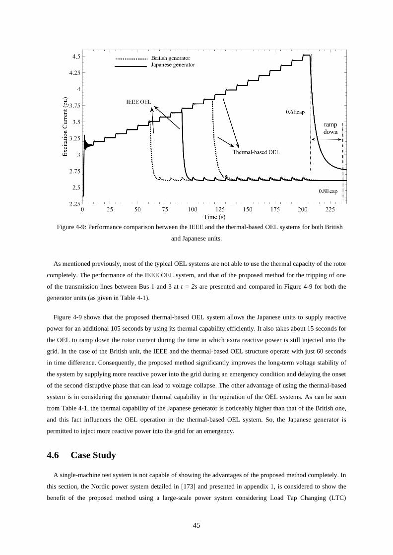
45

Figure 4-9: Performance comparison between the IEEE and the thermal-based OEL systems for both British

and Japanese units.

As mentioned previously, most of the typical OEL systems are not able to use the thermal capacity of the rotor

completely. The performance of the IEEE OEL system, and that of the proposed method for the tripping of one

of the transmission lines between Bus 1 and 3 at t = 2s are presented and compared in Figure 4-9 for both the

generator units (as given in Table 4-1).

Figure 4-9 shows that the proposed thermal-based OEL system allows the Japanese units to supply reactive

power for an additional 105 seconds by using its thermal capability efficiently. It also takes about 15 seconds for

the OEL to ramp down the rotor current during the time in which extra reactive power is still injected into the

grid. In the case of the British unit, the IEEE and the thermal-based OEL structure operate with just 60 seconds

in time difference. Consequently, the proposed method significantly improves the long-term voltage stability of

the system by supplying more reactive power into the grid during an emergency condition and delaying the onset

of the second disruptive phase that can lead to voltage collapse. The other advantage of using the thermal-based

system is in considering the generator thermal capability in the operation of the OEL systems. As can be seen

from Table 4-1, the thermal capability of the Japanese generator is noticeably higher than that of the British one,

and this fact influences the OEL operation in the thermal-based OEL system. So, the Japanese generator is

permitted to inject more reactive power into the grid for an emergency.

4.6 Case Study

A single-machine test system is not capable of showing the advantages of the proposed method completely. In

this section, the Nordic power system detailed in [173] and presented in appendix 1, is considered to show the

benefit of the proposed method using a large-scale power system considering Load Tap Changing (LTC)

46

transformers. The single line diagram of the Nordic power system is shown in Figure 4-10. In this system, loads

are modelled using the constant current model for active and reactive power. The LTC is also considered for all

transformers with the tap changing delay time varying from 8 to 12 seconds from one tap to another. Studies are

performed for single and multiple contingency cases to comprehensively show the features of the proposed

thermal-based OEL system.

Figure 4-10: Single line diagram of the Nordic power system [173].

The following assumptions are made for the case study of the Nordic power system:

1. All OEL systems are assumed to be current driven.

2. Conventional OEL systems timing is designed based on the information from [173].

3. The rotor resistor is 0.1 Ω for all generators.

4. The value of Ecap is adapted from the British generator thermal data scaled based on each generator

field current rated value and presented in appendix 1.

Case 1: Single contingency, the contingency considered is the 4032-4044 transmission line outage at t = 2s.

Initially, it is considered that the Nordic power system is equipped with the IEEE OEL system. So, after the

disturbance, the generators try to supply the emergency extra reactive power demand of the system by increasing

their excitation level as shown in Figure 4-11.

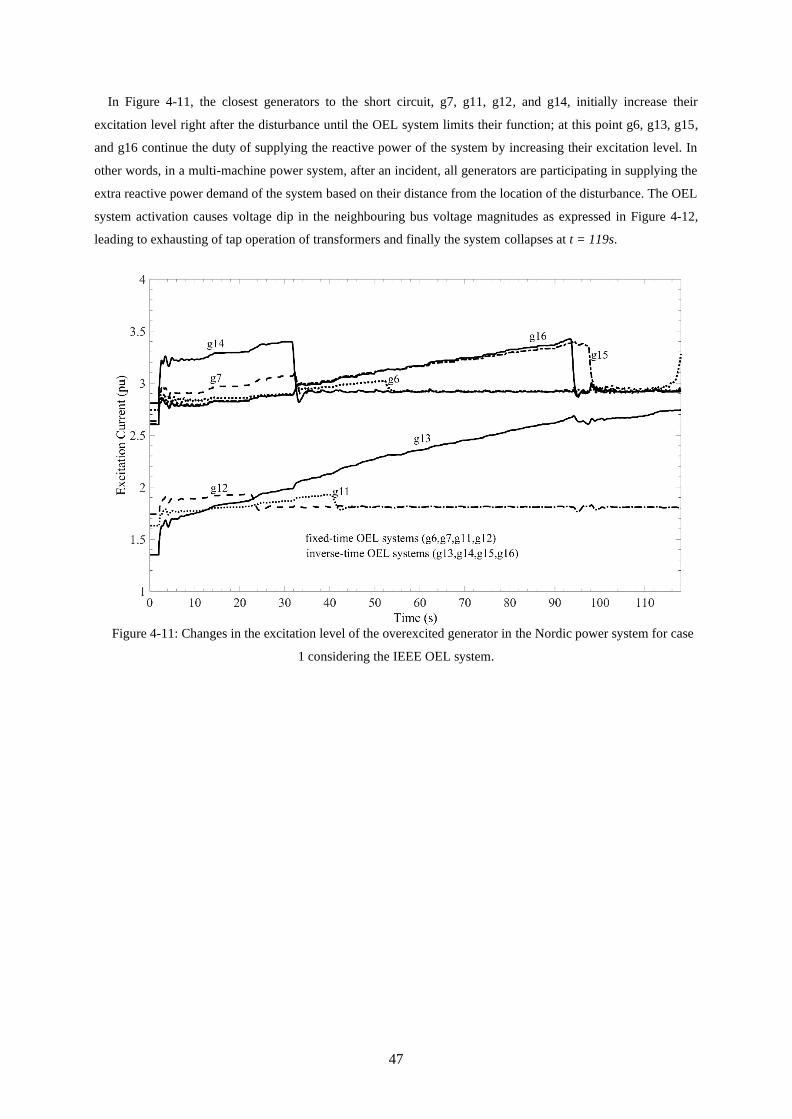
47

In Figure 4-11, the closest generators to the short circuit, g7, g11, g12, and g14, initially increase their

excitation level right after the disturbance until the OEL system limits their function; at this point g6, g13, g15,

and g16 continue the duty of supplying the reactive power of the system by increasing their excitation level. In

other words, in a multi-machine power system, after an incident, all generators are participating in supplying the

extra reactive power demand of the system based on their distance from the location of the disturbance. The OEL

system activation causes voltage dip in the neighbouring bus voltage magnitudes as expressed in Figure 4-12,

leading to exhausting of tap operation of transformers and finally the system collapses at t = 119s.

Figure 4-11: Changes in the excitation level of the overexcited generator in the Nordic power system for case

1 considering the IEEE OEL system.

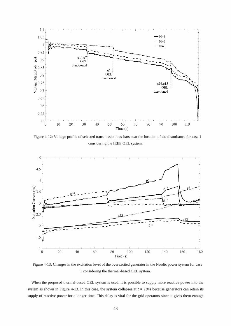
48


considering the IEEE OEL system.


1 considering the thermal-based OEL system.

When the proposed thermal-based OEL system is used, it is possible to supply more reactive power into the

system as shown in Figure 4-13. In this case, the system collapses at t = 184s because generators can retain its

supply of reactive power for a longer time. This delay is vital for the grid operators since it gives them enough

49

time to activate voltage related countermeasures.

Table 4-2: OEL systems activation time for case 1

Conventional OEL systems Thermal-based OEL systems

Improvement Gen

OEL functioning Time

(s) Gen OEL functioning Time (s)

g12 22.4 g14 73.6 325%

g14 31.6 g15 135.8 430%

g7 32.1 g16 154.6 480%

g11 40.5 g7 154.7 382%

g16 93.5 g6 Not Limited ∞

g15 97.2 g11 Not Limited ∞

g6 Not Limited g12 Not Limited 0%

Table 4-2 shows the time that OEL systems start reducing generator excitation levels for both IEEE and

thermal-based OEL systems. As is evident in Table 4-2, the OEL systems of the same generators get activated in

both IEEE and thermal-based cases, but, the order of activation is different; the conventional OEL systems are

activated based on their distance from the location of the event while the thermal-based OEL systems are

activated based on the thermal capacity of the generator in addition to its distance from the short circuit incident.

In this regards the voltage magnitudes of some affected buses are presented in Figure 4-14.


considering thermal-based OEL system.

In Figure 4-14, the voltage magnitudes start reducing after the disturbance with some minor dips mainly

because of the operation of LTCs, however, some major voltage dips can be also seen in the profile due to the

OEL limiting function in the nearby generators.

The operation of the LTCs has a significant role in the voltage stability of the system. The behaviour of the

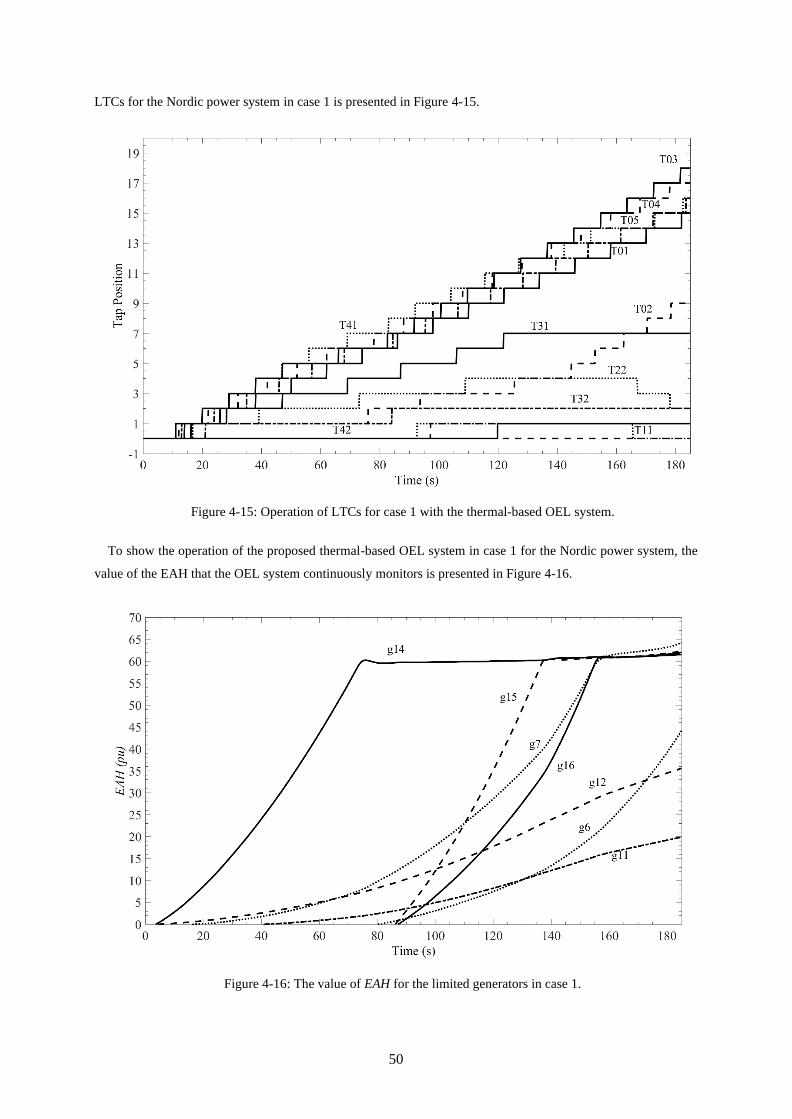
50

LTCs for the Nordic power system in case 1 is presented in Figure 4-15.

Figure 4-15: Operation of LTCs for case 1 with the thermal-based OEL system.

To show the operation of the proposed thermal-based OEL system in case 1 for the Nordic power system, the

value of the EAH that the OEL system continuously monitors is presented in Figure 4-16.

Figure 4-16: The value of EAH for the limited generators in case 1.

51

Case 2: Multiple contingencies, the contingency considered in this case is the outage of two 4044-4045

parallel lines; the first one at t = 2s and the second one at t = 16s. The excitation level of the generators

following the disturbance with conventional OEL system is presented in Figure 4-17.

Figure 4-17 shows that after the first line outage, the rotor currents of some affected generators slightly start

increasing until the second line outage, at which the rotor current of g7 suddenly increases. Because of the

significant increase in g7, its OEL system has functioned quickly and clamped the rotor current after 20 seconds;

which leads to the increase in the rotor current of g16. Sequentially, the OEL systems of g6 and g16 also operate

and limit the rotor current of the generators.


2 considering the IEEE OEL system.

Figure 4-18 shows that there is a major voltage dip in the profile when the OEL systems of g6 and g7 limit

their rotor currents. Another significant voltage drop also occurs at t = 82s; when, the OEL of g16 limits the

excitation current, resulting in the operation of the OLTCs; however, the system collapses at t = 135 s.

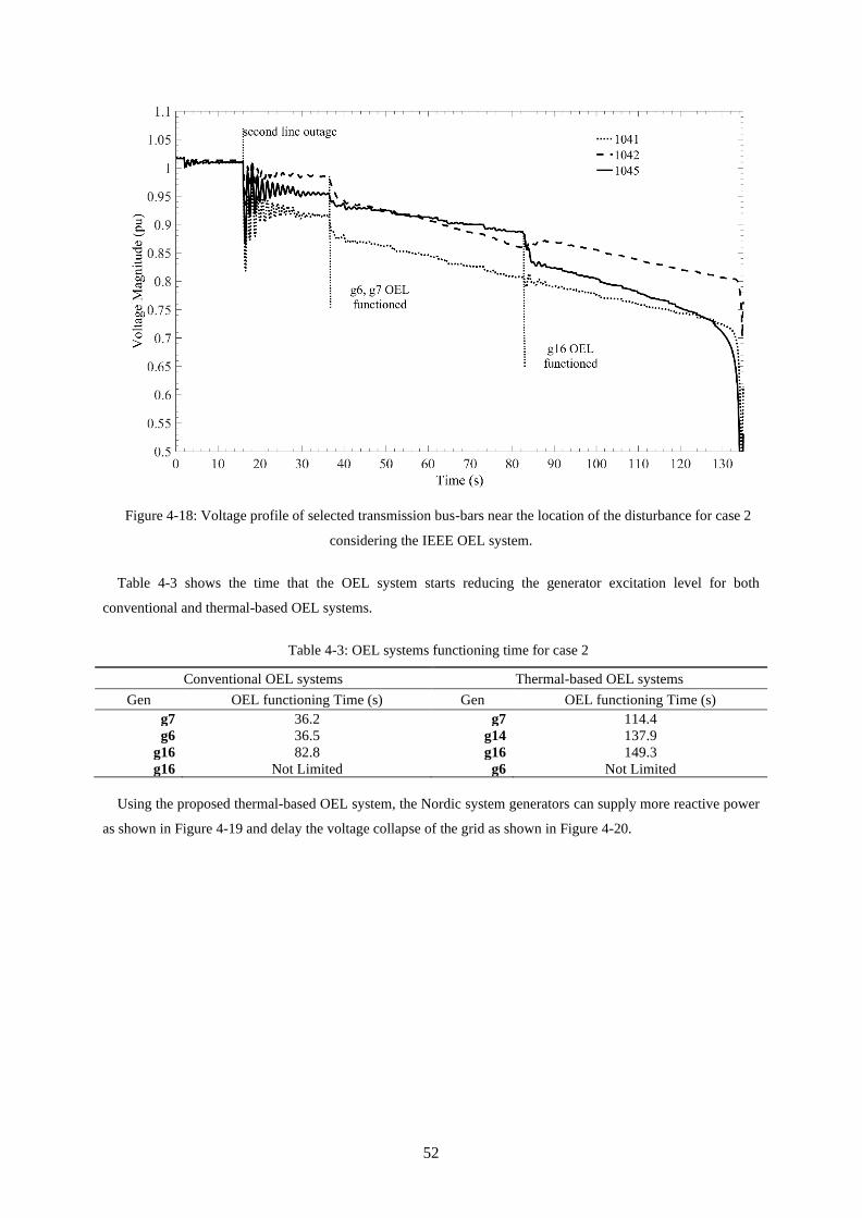
52


considering the IEEE OEL system.

Table 4-3 shows the time that the OEL system starts reducing the generator excitation level for both

conventional and thermal-based OEL systems.

Table 4-3: OEL systems functioning time for case 2

Conventional OEL systems Thermal-based OEL systems

Gen OEL functioning Time (s) Gen OEL functioning Time (s)

g7 36.2 g7 114.4

g6 36.5 g14 137.9

g16 82.8 g16 149.3

g16 Not Limited g6 Not Limited

Using the proposed thermal-based OEL system, the Nordic system generators can supply more reactive power

as shown in Figure 4-19 and delay the voltage collapse of the grid as shown in Figure 4-20.

53


2 considering the proposed thermal-based OEL system.


considering the proposed thermal-based OEL system.

Figures 4-19 and 4-20 show that considering the thermal-based OEL system, the generators were able to

supply reactive power for an extended time and delay the voltage collapse by 30s in the case on an n-1-1

contingency.

54

4.7 Summary

In this chapter, a new method is proposed for the determination of the timing for OEL activation, which is

developed based on available generator rotor thermal capacity. The performance of the proposed method is

validated using two test systems. Using the single-machine test system, the simulation result shows that the

proposed OEL method can efficiently utilize the thermal capacity of the rotor and inject more reactive power

into the system in comparison with that from a conventional OEL equipped generator.

The performance of the proposed method is further validated using the Nordic power system demonstrating its

effectiveness in extending the amount of reactive power that can be supplied in a multi-machine network

resulting in improved voltage stability of the system. The results from the Nordic power system show that all

generators participate in supplying the reactive power after a severe disturbance; the conventional OEL equipped

machines participate based on their electrical distance from the incident location while the thermal-based OEL

equipped units to participate by considering their thermal capacity in addition to their distance from the

disturbance. The generator owners may be able to be persuaded to allow more use of available reactive power

contribution of the generators to improve power system performance and voltage stability if incentives are

provided through the provision of ancillary and emergency control services in the electric power market.

A system protection scheme (SPS) using operational data from a SCADA system can be used to identify the

location and timing of impending voltage instability by observing a sudden increase of generator reactive power

outputs and the reduction of voltages in the area of disturbance. The benefit of the proposed thermal-based OEL

system is to increase the time for such an SPS to function, by increasing the time so that enough reactive power

can be injected into the grid. This will provide the SPS more time to determine the best countermeasure that can

be effective to mitigate the emergency condition.

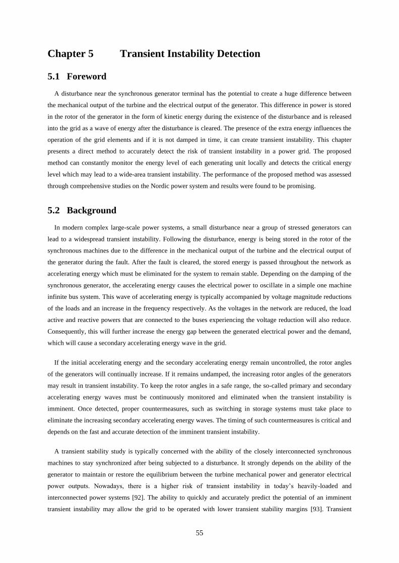
55

Chapter 5 Transient Instability Detection

5.1 Foreword

A disturbance near the synchronous generator terminal has the potential to create a huge difference between

the mechanical output of the turbine and the electrical output of the generator. This difference in power is stored

in the rotor of the generator in the form of kinetic energy during the existence of the disturbance and is released

into the grid as a wave of energy after the disturbance is cleared. The presence of the extra energy influences the

operation of the grid elements and if it is not damped in time, it can create transient instability. This chapter

presents a direct method to accurately detect the risk of transient instability in a power grid. The proposed

method can constantly monitor the energy level of each generating unit locally and detects the critical energy

level which may lead to a wide-area transient instability. The performance of the proposed method was assessed

through comprehensive studies on the Nordic power system and results were found to be promising.

5.2 Background

In modern complex large-scale power systems, a small disturbance near a group of stressed generators can

lead to a widespread transient instability. Following the disturbance, energy is being stored in the rotor of the

synchronous machines due to the difference in the mechanical output of the turbine and the electrical output of

the generator during the fault. After the fault is cleared, the stored energy is passed throughout the network as

accelerating energy which must be eliminated for the system to remain stable. Depending on the damping of the

synchronous generator, the accelerating energy causes the electrical power to oscillate in a simple one machine

infinite bus system. This wave of accelerating energy is typically accompanied by voltage magnitude reductions

of the loads and an increase in the frequency respectively. As the voltages in the network are reduced, the load

active and reactive powers that are connected to the buses experiencing the voltage reduction will also reduce.

Consequently, this will further increase the energy gap between the generated electrical power and the demand,

which will cause a secondary accelerating energy wave in the grid.

If the initial accelerating energy and the secondary accelerating energy remain uncontrolled, the rotor angles

of the generators will continually increase. If it remains undamped, the increasing rotor angles of the generators

may result in transient instability. To keep the rotor angles in a safe range, the so-called primary and secondary

accelerating energy waves must be continuously monitored and eliminated when the transient instability is

imminent. Once detected, proper countermeasures, such as switching in storage systems must take place to

eliminate the increasing secondary accelerating energy waves. The timing of such countermeasures is critical and

depends on the fast and accurate detection of the imminent transient instability.

A transient stability study is typically concerned with the ability of the closely interconnected synchronous

machines to stay synchronized after being subjected to a disturbance. It strongly depends on the ability of the

generator to maintain or restore the equilibrium between the turbine mechanical power and generator electrical

power outputs. Nowadays, there is a higher risk of transient instability in today’s heavily-loaded and

interconnected power systems [92]. The ability to quickly and accurately predict the potential of an imminent

transient instability may allow the grid to be operated with lower transient stability margins [93]. Transient

56

stability assessment in the power system has always been a major part of the power system analysis [94]. The

transient stability of a power system can be assessed through energy methods or time-domain simulations.

The development in parallel computing techniques has improved the efficiency of the time domain simulation-

based methods to be able to handle large-scale power system transient stability assessment [95], [96]. In [174] an

approach is proposed that indicates the assessment result before the computationally demanding time-domain

studies are finished. The trajectory sensitivity methods based on time-domain simulations have also been used in

the determination of power flow limits and dynamic VAr planning [175], [176]. Besides, the developments in

computation power have also directly impacted the use of pattern recognition methods to predict transient

stability issues based on the information provided through PMUs [97]. An innovative online transients stability

assessment method based on machine learning that uses PMUs has been presented in [177]. An innovative wide-

area supplementary controller that uses a nonlinear Kalman filter to eliminate the local modes as measurement

noises using a controllable series compensator is introduced in [100] and then is developed in [101] to use SVCs.

Considering the increasing penetration of the inverter-based generating plants and electric vehicles, a global

and innovative method has been proposed that integrates the global transient energy function and re-closer

probability distribution functions to provide a quantitative measure of the probability of stability [99]. An

efficient transient stability assessment method for inverter-based generation considering the phase lock loop has

been introduced in [178].

The transient stability of a multi-machine power system can also be investigated from the distinctive

individual machine standpoint [103], [104]. The individual machine energy function method was derived by

considering the individual-machine perspective, where the stability of the system is determined by individual

machine energy functions [105], [106]. In [108], [109], [179], a detailed transient stability analysis of multi-

machine power systems is performed for each individual machine, and the required energy of the selected local

countermeasures was calculated using the partial energy function. In [110], the transient stability margin of the

system is identified using a combination of equal area criteria of the critical machine and partial energy function.

To efficiently determine the transient stability of a power system in the multi-machine environment, a

synchronous referred individual machine energy function has also been used [111] and aided in computing the

system's critical clearing time during the transients in [112].

The proposed transient instability detection method in the chapter is a direct time-domain method based on the

individual machine’s participation in the transient instability of the wide-area power grid. In the proposed

method, the excess energy (the gap between the mechanical output of the turbine and the electrical output of the

generator) injected into the grid during a contingency is measured online continuously for each critical individual

generating unit within the wide-area network at the generating unit terminal. To describe the relationship

between the excess energy of each individual generating unit and the wide-area transient stability, two new

variables as the Primary Accelerating Energy (PAE) and the Secondary Accelerating Energy (SAE) are defined.

The PAE is created by an individual generating unit during the disturbance, then the PAE is injected into the grid

and is converted into the SAE. The SAE is then kept spreading into the grid in the post-contingency condition

and causes wide-area transient instability. The SAE can be divided into two parts, the first part is caused by

PAE, and, the second part that contains a wide-area (wave-like) characteristics. If the first part of the SAE

57

remains uncontrolled, the second part can cause wide-area transient instability. The proposed method measures

the value of PAE at each generating unit terminal and detects if the PAE will lead to an uncontrollable SAE and

causes transient instability.

5.3 Accelerating Energy in a Power System

The transient energy of the system after a disturbance in a power grid has been investigated in [81], [98], [103]

and presented in (5-1);

( ),i i K P

E E E = − (5-1)

Where

21

2K eq eq

E M = (5-2)

And

( ) ( ) ( )1 1

1 1 1

cos cos sin sin

s sm m mi i j js s s

P ei i i ij ij ij ij ij ijsi i j i ij ij

E P C D

− −

= = = +

− + −= − + − + −

− (5-3)

where, E is the total accelerating energy, ωi is the ith generator speed, δi, is the ith generator angle, EK, is the

kinetic energy, EP is the potential energy, Meq is the equivalent moment of inertia, ωeq is the equivalent speed, Pei

is the output electrical power of the ith generator, δis is the post-contingency equilibrium point angle of the ith

generator and δij = δi – δj and,

2

ei mi i iiP P E G= −

(5-4)

ij i j ijC E E B= (5-5)

ij i j ijD E E G= (5-6)

where Pmi is the output mechanical power of the ith generator, Ei is the generator field voltage of the ith generator,

Bij, Gij is the susceptance and the conductance, between the ith and the jth generator.

Based on (5-1), the total energy in the wide-area power grid is formed by the combination of the potential and

kinetic energy. The potential energy cannot be directly measured in the network, however, the kinetic energy can

be calculated at the generating unit terminals as the generating plants are the only sources of energy in the grid.

For the generating units, the kinetic energy difference between the turbine output mechanical energy and the

generator output electrical energy at each instance of time is the PAE. The physical concept of the PAE can be

simply presented from the classical swing equation expressed in (5-7).

58

2

2

2sys m e

sys

H d dD P P

dt dt

+ = − (5-7)

where H is the system inertia constant, ωsys is the system speed, δ is the generator rotor angle, D is the rotor

damping constant, Pm is the turbine output mechanical power and Pe is the generator output electrical power.

Under a normal operating condition, the right-hand side of (5-7) should be equal to zero, which means that the

synchronous machine speed will remain constant (because the acceleration is zero), and there will be no

deviations in the rotor angle. Based on (5-7), considering constant mechanical power output from the prime

mover, in the case of any deviation in the value of Pe, the right-hand side of (5-7) will become non-zero which

means that there would be acceleration (Pm – Pe > 0) or deceleration (Pm – Pe < 0) on the rotor of the

synchronous machine.

To assess the impact of the PAE from an individual generating unit on the grid, the dynamic reaction of a

synchronous generator connected to a load substation has been investigated prior, during and after a three-phase

to ground solid short circuit at the generator terminal as shown in Figure 5-1. In Figure 5-1, Pe is measured at

generator terminal and PL and VL are measured at the load substation. In Figure 5-1, during pre-contingency,

between t0 and t1; Pm, Pe and load power demand (PL) is equal to 1pu. At t1, a three-phase to ground solid short

circuit happens and Pe and PL become zero, while Pm remains 1pu until t2. The mismatch between Pm and Pe

during the fault causes the PAE to become non-zero.

The right-hand side of (5-7) indicates the difference between the mechanical power output of the turbine and

the electrical power output of the generator. Let us call it Pacc, the acceleration power, as shown in (5-8);

acc m eP P P= −

(5-8)

In the normal operating condition (between t0 and t1), the value of Pacc equals to zero; however, between t1 and

t2, the value of Pm is higher than Pe producing a positive acceleration power (Pacc > 0) increasing the rotor speed

and consequently increasing the rotor angle. To obtain the amount of stored energy in the rotor of the generator

as a result of the Pacc, equation (5-8) should be integrated through time as expressed in (5-9);

( )acc m eP dt P P dt= − (5-9)

By calling the left-hand side of (5-9) the primary accelerating energy, PAE, it can be expressed as (5-10):

( )PAEm e

P P dt= − (5-10)

The PAE can be simply calculated using (5-10). As indicated in (5-10), the value of the PAE is calculated

locally at the generator terminal and only depends on the individual generating unit. The PAE does not represent

any wide-area network energy level indication and it only shows how much excess energy has been injected into

the wide-area network by the individual generating unit as a result of the disturbance. Monitoring the value of

PAE is the first step in identifying if a generating unit injects excess energy into the grid and increases the risk of

59

transient instability.

After the fault is cleared at t2, the electrical power is restored to its initial condition and the PAE becomes

zero. In post-contingency (after t2), the excess energy injected into the grid as the PAE increases output electrical

power of the generator (Pe), causes a power gap between, Pe and the active power demand of the load (PL),

igniting the first part of the SAE. The first part of the SAE is caused by the individual generating unit response in

the post-contingency situation as illustrated in Figure 5-1.

Figure 5-1: Mechanical, electrical and load power, and load voltage subjected to a 3Ph-G fault where load power

is assumed to be independent of load voltage.

To calculate the first part of the SAE, the accelerating power (Pacc) should be determined as given by;

acc e LP P P= −

(5-11)

By integrating (5-11) for time, the first part of the SAE is calculated in (5-12),

( )SAEe L

P P dt= − (5-12)

This first part of the SAE is caused by the generator as the generator output power is changing as a response to

the disturbance and will return to its pre-contingency value after some time, depending on the damping of the

generator; consequently, the first part of the SAE is a temporary characteristic.

The increase in the Pe due to the PAE (first part of the SAE) has a second negative impact on the transient

stability of the network. As Pe increase, the losses on the transmission line increase and the voltage at the load

zone substation decreases. The reduction in the voltage magnitude of the load reduces the maximum electrical

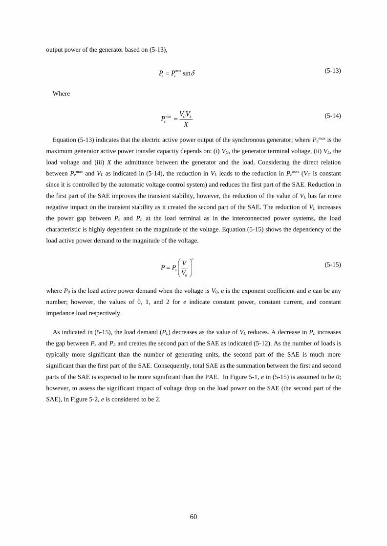
60

output power of the generator based on (5-13),

max sine e

P P = (5-13)

Where

max G L

e

V VP

X=

(5-14)

Equation (5-13) indicates that the electric active power output of the synchronous generator; where Pemax is the

maximum generator active power transfer capacity depends on: (i) VG, the generator terminal voltage, (ii) VL, the

load voltage and (iii) X the admittance between the generator and the load. Considering the direct relation

between Pemax and VL as indicated in (5-14), the reduction in VL leads to the reduction in Pe

max (VG is constant

since it is controlled by the automatic voltage control system) and reduces the first part of the SAE. Reduction in

the first part of the SAE improves the transient stability, however, the reduction of the value of VL has far more

negative impact on the transient stability as it created the second part of the SAE. The reduction of VL increases

the power gap between Pe and PL at the load terminal as in the interconnected power systems, the load

characteristic is highly dependent on the magnitude of the voltage. Equation (5-15) shows the dependency of the

load active power demand to the magnitude of the voltage.

0

0

e

VP P

V

=

(5-15)

where P0 is the load active power demand when the voltage is V0, e is the exponent coefficient and e can be any

number; however, the values of 0, 1, and 2 for e indicate constant power, constant current, and constant

impedance load respectively.

As indicated in (5-15), the load demand (PL) decreases as the value of VL reduces. A decrease in PL increases

the gap between Pe and PL and creates the second part of the SAE as indicated (5-12). As the number of loads is

typically more significant than the number of generating units, the second part of the SAE is much more

significant than the first part of the SAE. Consequently, total SAE as the summation between the first and second

parts of the SAE is expected to be more significant than the PAE. In Figure 5-1, e in (5-15) is assumed to be 0;

however, to assess the significant impact of voltage drop on the load power on the SAE (the second part of the

SAE), in Figure 5-2, e is considered to be 2.

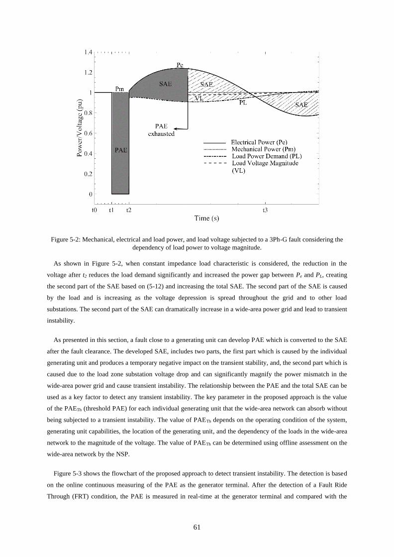
61

Figure 5-2: Mechanical, electrical and load power, and load voltage subjected to a 3Ph-G fault considering the

dependency of load power to voltage magnitude.

As shown in Figure 5-2, when constant impedance load characteristic is considered, the reduction in the

voltage after t2 reduces the load demand significantly and increased the power gap between Pe and PL, creating

the second part of the SAE based on (5-12) and increasing the total SAE. The second part of the SAE is caused

by the load and is increasing as the voltage depression is spread throughout the grid and to other load

substations. The second part of the SAE can dramatically increase in a wide-area power grid and lead to transient

instability.

As presented in this section, a fault close to a generating unit can develop PAE which is converted to the SAE

after the fault clearance. The developed SAE, includes two parts, the first part which is caused by the individual

generating unit and produces a temporary negative impact on the transient stability, and, the second part which is

caused due to the load zone substation voltage drop and can significantly magnify the power mismatch in the

wide-area power grid and cause transient instability. The relationship between the PAE and the total SAE can be

used as a key factor to detect any transient instability. The key parameter in the proposed approach is the value

of the PAETh (threshold PAE) for each individual generating unit that the wide-area network can absorb without

being subjected to a transient instability. The value of PAETh depends on the operating condition of the system,

generating unit capabilities, the location of the generating unit, and the dependency of the loads in the wide-area

network to the magnitude of the voltage. The value of PAETh can be determined using offline assessment on the

wide-area network by the NSP.

Figure 5-3 shows the flowchart of the proposed approach to detect transient instability. The detection is based

on the online continuous measuring of the PAE as the generator terminal. After the detection of a Fault Ride

Through (FRT) condition, the PAE is measured in real-time at the generator terminal and compared with the

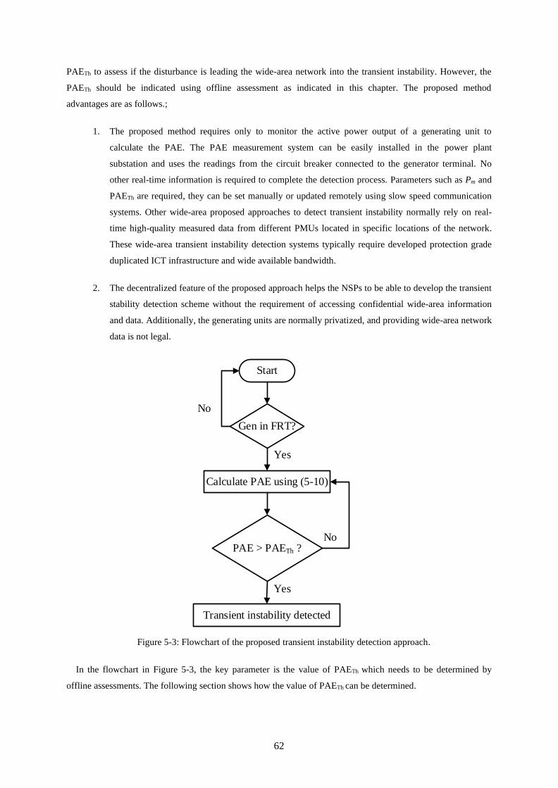
62

PAETh to assess if the disturbance is leading the wide-area network into the transient instability. However, the

PAETh should be indicated using offline assessment as indicated in this chapter. The proposed method

advantages are as follows.;

1. The proposed method requires only to monitor the active power output of a generating unit to

calculate the PAE. The PAE measurement system can be easily installed in the power plant

substation and uses the readings from the circuit breaker connected to the generator terminal. No

other real-time information is required to complete the detection process. Parameters such as Pm and

PAETh are required, they can be set manually or updated remotely using slow speed communication

systems. Other wide-area proposed approaches to detect transient instability normally rely on real-

time high-quality measured data from different PMUs located in specific locations of the network.

These wide-area transient instability detection systems typically require developed protection grade

duplicated ICT infrastructure and wide available bandwidth.

2. The decentralized feature of the proposed approach helps the NSPs to be able to develop the transient

stability detection scheme without the requirement of accessing confidential wide-area information

and data. Additionally, the generating units are normally privatized, and providing wide-area network

data is not legal.

No

Calculate PAE using (5-10)

PAE > PAETh ?

Transient instability detected

Yes

Gen in FRT?

Yes

Start

No

Figure 5-3: Flowchart of the proposed transient instability detection approach.

In the flowchart in Figure 5-3, the key parameter is the value of PAETh which needs to be determined by

offline assessments. The following section shows how the value of PAETh can be determined.

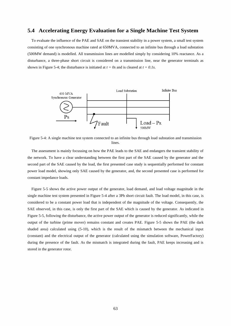
63

5.4 Accelerating Energy Evaluation for a Single Machine Test System

To evaluate the influence of the PAE and SAE on the transient stability in a power system, a small test system

consisting of one synchronous machine rated at 650MVA, connected to an infinite bus through a load substation

(500MW demand) is modelled. All transmission lines are modelled simply by considering 10% reactance. As a

disturbance, a three-phase short circuit is considered on a transmission line, near the generator terminals as

shown in Figure 5-4; the disturbance is initiated at t = 0s and is cleared at t = 0.1s.

Figure 5-4: A single machine test system connected to an infinite bus through load substation and transmission

lines.

The assessment is mainly focussing on how the PAE leads to the SAE and endangers the transient stability of

the network. To have a clear understanding between the first part of the SAE caused by the generator and the

second part of the SAE caused by the load, the first presented case study is sequentially performed for constant

power load model, showing only SAE caused by the generator, and, the second presented case is performed for

constant impedance loads.

Figure 5-5 shows the active power output of the generator, load demand, and load voltage magnitude in the

single machine test system presented in Figure 5-4 after a 3Ph short circuit fault. The load model, in this case, is

considered to be a constant power load that is independent of the magnitude of the voltage. Consequently, the

SAE observed, in this case, is only the first part of the SAE which is caused by the generator. As indicated in

Figure 5-5, following the disturbance, the active power output of the generator is reduced significantly, while the

output of the turbine (prime mover) remains constant and creates PAE. Figure 5-5 shows the PAE (the dark

shaded area) calculated using (5-10), which is the result of the mismatch between the mechanical input

(constant) and the electrical output of the generator (calculated using the simulation software, PowerFactory)

during the presence of the fault. As the mismatch is integrated during the fault, PAE keeps increasing and is

stored in the generator rotor.

64

Figure 5-5: Generator output and load power of the single machine test system in the stable first swing

considering constant power load model.

In Figure 5-6, the energy levels caused by the generating unit during and after the disturbance in the test

system is presented. Here, PAE is increased up to 0.1pu during the fault and then is released into the grid as SAE

which is increased up to 0.175pu. The SAE in this case caused by the generator only. The system transient

stability for this case has been preserved and the network was able to dissipate the PAE injected by the

generating unit.


65

considering constant power load.

The results in Figure 5-7, shows the test system characteristic to the same disturbance as the previous case

when the constant impedance load model is considered. Using the constant impedance load model, the load

demand is highly dependent on the magnitude of load voltage. After the fault clearance at t = 0.1s, the generator

accelerates due to the stored kinetic energy in its rotor as a result of the PAE developed during the fault. The

generator rotor angle and the output power are increased which leads to an overloading behaviour in the

remaining transmission lines, pushing the angle wider across them and increasing the line current and losses.

This leads to a progressive drop in the voltage magnitude of the load substations despite the generator terminal

voltage is kept constant by the generator automatic voltage regulator. As the constant impedance load model

proportional to the square of voltage magnitude, the second part of the SAE becomes non-zero. In Figure 5-6,

SAE is caused due to both reduction of the Pemax based on (5-14) as well as the reduction of the load demand

caused by voltage depression in the load substation.

Figure 5-7: Generator output power and load power of the single machine test system in the stable first swing

considering constant impedance load.

As shown in Figure 5-6, the load active power demand reduces to zero and then is restored to 96% after the

fault is cleared. As the generator rotor angle increases, the generator active power output increases, the voltage

decreases furthermore, reducing the load to 88% at t = 0.49s. During the first swing, the voltage is reduced, and

the load is diminished consequently leaving a big power gap between the generator output power and the load

power as indicated in Figure 5-7 as a shaded area.

Similar to Figure 5-6, Figure 5-8 shows the PAE and the total SAE, but, when the load is modelled as a

constant impedance load. As shown in Figure 5-8, in addition to the SAE caused by the generator response to the

disturbance, reduction in the load demand has also contributed to the SAE and increased the total SAE

66

significantly in comparison with Figure 5-6.

Figure 5-8: Primary and secondary acceleration energy of the single machine test system in the stable first

swing with the constant impedance load model.

In Figure 5-8, it can be concluded that the SAE from the generator (a temporary impact) is decreasing after the

peak at t = 0.9s, while the value of SAE caused by the load reduction (permanent impact) is constantly

increasing.

Using the same test system, the fault clearance has been extended from 5 cycles to 10 cycles (0.2 seconds).

Figure 5-9 shows the characteristics of the single machine test system considering the extended clearance time.

67

Figure 5-9: Generator output power and load power of the single machine test system in the unstable first


In Figure 5-8, the fault is cleared at t = 0.2s, however, the load voltage and the power have been dropped

dramatically when compared with Figure 5-7. The PAE and SAE the extended fault clearance time is calculated

and presented in Figure 5-10. Increasing the fault clearance time causes the PAE stored in the rotor of the

generator to be doubled (0.2pu). After the fault is cleared, the PAE is injected into the network and creates SAE.

As SAE passes through the substation, it is multiplied and the second part of the SAE caused by the load voltage

reduction increases dramatically.

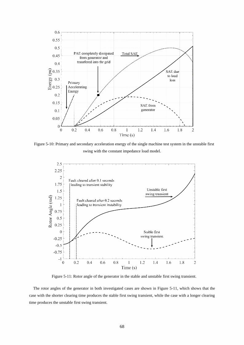
68

Figure 5-10: Primary and secondary acceleration energy of the single machine test system in the unstable first


Figure 5-11: Rotor angle of the generator in the stable and unstable first swing transient.

The rotor angles of the generator in both investigated cases are shown in Figure 5-11, which shows that the

case with the shorter clearing time produces the stable first swing transient, while the case with a longer clearing

time produces the unstable first swing transient.

69

Technically, it can be stated that the test system in Figure 5-3 is capable of handling the PAE value of 0.1pu

and cannot handle the PAE value of 0.2pu. This PAE (0.2pu) can be used as PAETh as indicated in the proposed

transient detection approach resented in Figure 5-3. The capability of the system in managing the excess energy

can be used efficiently to indicate the risk of transient stability of a network. This indication can also be used to

improve the transient stability of a network by considering countermeasures such as using storage systems or

increase the capability of the system in eliminating the PAE at the generating unit terminal. The value of PAETh

can also be used to select the size of the required countermeasure to be installed.

5.5 Performance Evaluation through Case Studies

The proposed method has been applied to the Nordic power system and its performance investigated. In this

section, the Nordic power system has been selected as the test system to assess each generating unit individual

impact on the wide-area transient stability. Additionally, the whole grid energy level has been calculated only as

an indicator of how each generating unit participates in the Nordic power system energy level. Using the Nordic

power system, the PAE injected into the network by each individual generating unit and its impact on the Nordic

system are assessed. The disturbance is a solid three-phase short circuit on one of the transmission lines

connecting buses 4062 and 4063 in the southern region of the Nordic power system as shown in Figure 5-12.

Figure 5-12: Single line diagram of the Nordic power system.

The disturbance is initiated at t = 0s and cleared after 5 cycles (t = 0.1s) and the simulation results show that

the system produces stable first swing condition, however when the clearing time is delayed and the fault is

70

cleared after 9 cycles (t = 0.18s), the system produces unstable first swing condition.

Figure 5-13 shows the deviation in the active power output of G18, G17, G15, and G08, which are the closest

generators to the location of the disturbance. Figure 5-13 indicates that the PAE stored in the rotor of G18 during

the disturbance was able to push the power output by 33% at t = 0.72s in post-contingency; moreover, the PAE

generated by G18 keeps spreading into the grid as a wave of energy, increasing the output power of G17, G15

and G08 by 20%, 9% and 4% at t = 0.92s, 1.05s and 1.09. The output powers of the nearby generators keep

increasing during the first swing. These generators are selected to be the critical generators in the Nordic power

system for this specific disturbance.

Figure 5-13: Selected generators output power of Nordic power system in the stable first swing.

The extra generated power by G17, G15, and G08 will ignite the SAE as presented in Figure 5-14. Figure 5-14

shows the SAE caused by G18, G17, G15, and G08 and the total SAE in the post-contingency condition. The

value of the total SAE caused by the generators extra-generated power is 0.27pu, while the total PAE stored

during the disturbance is 0.17pu. The value of SAE is more significant that the PAE. The calculated total PAE

and SAE are calculated by the summation of G18, G17, G15 and G08 PAE and SAE, consequently, the total

PAE and SAE only represents these 4 generating units and not all Nordic system. The total PAE and total SAE

have only been presented as indicative values. In the proposed approach to detect transient instability, the total

PAE and total SAE are not required. Other factors such as coherent groups also contribute to the transient

instability, however, in this work, only the contribution of each generating unit has been considered individually

and the interaction between the machines are not considered.

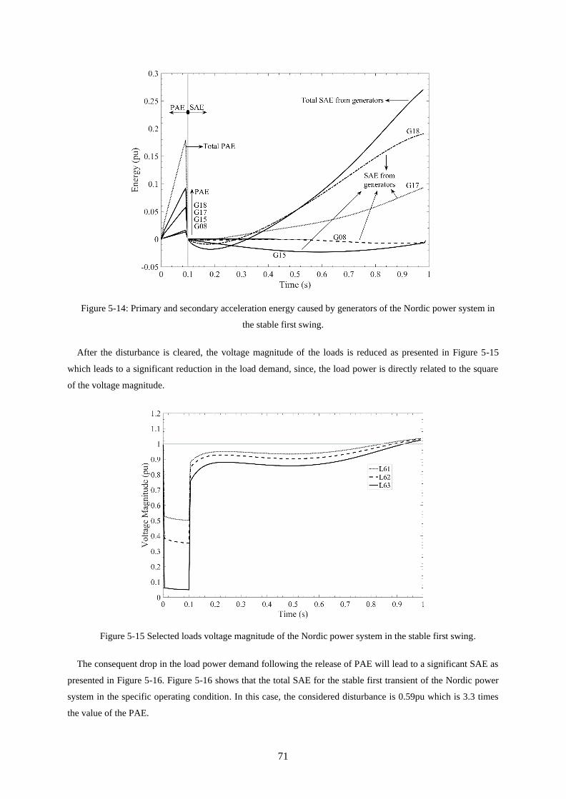
71

Figure 5-14: Primary and secondary acceleration energy caused by generators of the Nordic power system in

the stable first swing.

After the disturbance is cleared, the voltage magnitude of the loads is reduced as presented in Figure 5-15

which leads to a significant reduction in the load demand, since, the load power is directly related to the square

of the voltage magnitude.

Figure 5-15 Selected loads voltage magnitude of the Nordic power system in the stable first swing.

The consequent drop in the load power demand following the release of PAE will lead to a significant SAE as

presented in Figure 5-16. Figure 5-16 shows that the total SAE for the stable first transient of the Nordic power

system in the specific operating condition. In this case, the considered disturbance is 0.59pu which is 3.3 times

the value of the PAE.

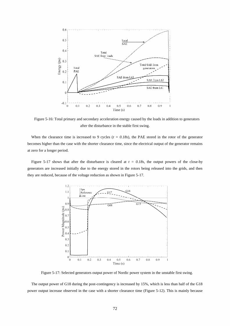
72

Figure 5-16: Total primary and secondary acceleration energy caused by the loads in addition to generators

after the disturbance in the stable first swing.

When the clearance time is increased to 9 cycles (t = 0.18s), the PAE stored in the rotor of the generator

becomes higher than the case with the shorter clearance time, since the electrical output of the generator remains

at zero for a longer period.

Figure 5-17 shows that after the disturbance is cleared at t = 0.18s, the output powers of the close-by

generators are increased initially due to the energy stored in the rotors being released into the grids, and then

they are reduced, because of the voltage reduction as shown in Figure 5-17.

Figure 5-17: Selected generators output power of Nordic power system in the unstable first swing.

The output power of G18 during the post-contingency is increased by 15%, which is less than half of the G18

power output increase observed in the case with a shorter clearance time (Figure 5-12). This is mainly because

73

the rotor angles of the generators were already unstable in its first swing as shown in Figure 5-17. The rotor

angle of the affected generator is presented in Figure 5-18.

Figure 5-18: Rotor angle of the generators for the Nordic power system in the stable and unstable first swing.

Due to the longer presence of the disturbance, in the first swing as shown in Figure 5-19, the total PAE value

calculated by summation of the PAE’s from G18, G17, G15 and G08 has been increased to 0.33pu. This

significant difference between the stable and unstable first swing value of the total PAE was occurred due to the

increasing values of the rotor angles of the generators in the unstable swing (shown in Figure 5-18) caused by the

delayed fault clearance.

However, the value of the total SAE calculated by the summation of the SAE’s from G18, G17, G15, and G08

was reduced to -0.13pu, and the generators helped the transient stability of the network by reducing the value of

their SAE. Since generators’ post-contingency characteristics have contributed to reduce the value of SAE, it is

not efficient to use a countermeasure to dissipate more energy at the generator point of connections.

74

Figure 5-19: Primary and secondary acceleration energy caused by generators after the disturbance in the

unstable first swing.

The value of PAE for each generating unit measured in Figure 5-19 can be used as the PAETh for each of the

G18, G17, G08, and G15 generating units. Based on the proposed transient instability detection method, when

the PAETh for each critical generating unit is reached, transient instability is imminent.

The voltage drops in the load bus-bars after the disturbance in the unstable first swing situation are given in

Figure 5-20. As it is evident, the voltage drop is very significant and leads to a significant reduction in the load

demand and a significant increase in the SAE caused by the load.

Figure 5-20: Selected loads voltage magnitude of the Nordic power system in the unstable first swing.

Figure 5-21 shows that the negative SAE due to the generators has reduced the total value of SAE from 1.15

75

(SAE due to the loads) to 1.02. However, the SAE after 1 second is still 3.1 times greater than the PAE and leads

to transient instability. By reducing the SAE caused by the loads, transient stability can be maintained.

Figure 5-21: Total primary and secondary acceleration energy caused by the loads in addition to generators

after the disturbance in the unstable first swing.

A comparison between the SAE due to the generators and the SAE due to the loads shows that the SAE due to

the load demand reduction impacts the network transient stability more significantly. This fact can be used in

developing efficient countermeasures with the idea of increasing the SAE reduction rate at the load zone

substations. The developed countermeasures should be located at the load buses to compensate for the reduced

load demand and hence to reduce the SAE imposed by load reduction. Ideally, by removing the SAE caused by

the load reduction, the system can preserve its stability. Consequently, the reduction in the load (the dependency

of the load demand to voltage magnitude) can be used as an indicator to find out how much more energy needs

to be eliminated to achieve zero SAE. One of the potential countermeasures is to switch in energy storage

systems installed in the load buses to reduce the SAE.

5.6 Summary

This chapter has presented a direct method to quickly and accurately detect the potential risk of an imminent

transient instability in a power system by monitoring the excess energy injected into the grid by each individual

generating unit. The proposed method first calculates the primary accelerating energy for each generator during

the fault and then compares it with a threshold to indicate if the injected accelerating energy leads to transient

instability. As the wave of energy passes through the network, the secondary accelerating energy keeps

increasing and the rotor angles of the generators move further away from the normal operating angles. To

facilitate the proposed method, the power gap between the active power at the generator terminal and the active

power at the load substation feeder should be assessed offline and the primary accelerating energy threshold

determined by the NSP. This can be used to calculate the excess energy created by each generating unit in the

grid which makes it practical and simple to implement. The proposed method can be used to assess whether a

76

network is close to the transient instability. The method can also be used in real time to detect the risk of

transient instability and estimate the available time for applying the countermeasures.

77

Chapter 6 Transient Stability Improvement

6.1 Foreword

In this chapter, a new approach is presented to reduce the nonlinear characteristics of a stressed power system

and improve the transient stability of the system by reducing its second-order modal interaction through retuning

selected critical parameters of the generator excitation system. To determine the magnitude of the second-order

modal interaction within the system, a new index on nonlinearity is developed using normal form theory. Using

the proposed index of nonlinearity, a sensitivity function is formed to indicate the most effective excitation

system parameters in the nonlinear behaviour of the system. These dominant parameters are tuned to reduce the

magnitude of the second-order modal interaction of the system and to reduce the index on nonlinearity. The

efficiency of the proposed method is initially validated using a four-machine two-area test system. The IEEE 39-

Bus New England test system is then used to investigate the performance of the proposed method for a more

realistic system. Simulation results show that a proper tuning of the excitation controller can reduce the

magnitude of the second-order modal interaction of the system and can even improve the transient stability

margin of the network.

6.2 Background

Today power systems are increasingly stressed due to the continuously growing load as the penetration of

plug-in electric vehicles (PEV) is increased; moreover, PEV charging stations and controller are naturally highly

nonlinear loads and connecting them to the power grid increases the nonlinearity of the system [180], [181].

Under such a stressed condition, the conventional local linear model tested only at equilibrium points may fail to

model the complete system characteristics or may reveal incomplete system performance. Further, as the system

becomes more stressed, complicated phenomena involving the interaction between the system modes may occur

[115]. As discussed in [117], the interaction between modes plays an important role in the dynamic

characteristics of the system and must be considered in comprehensive dynamic studies.

In the late eighties, attempts to consider the nonlinear characteristics and modal interaction of the system were

initiated. In [115] and [116], the envelope equation, which governs the aspect of the resonance between two

modes, is presented. In [117], the inter-area mode phenomenon in stressed power systems following large

disturbances is studied. The importance of adding the second-order terms in a time-domain simulation is

presented in [118]. In the same year, the Normal Form (NF) theory is used as a tool to identify the nonlinear

aspects of the modal interaction phenomenon [182].

The NF theory is a useful and powerful analytical tool to study the characteristic of a nonlinear dynamical

system in the neighbourhood of an equilibrium point. Over the past few years, NF has been widely used to

determine the effect of the modal interaction on the controller’s performance [120]–[122]. In [123], [183], some

guidelines were presented to design system controllers to reduce the inter-area oscillation of the system using

NF. NF has also been used to indicate the effect of modal interactions on machine states, system participation

factors, and eigenvectors [124], [125]. In a stressed power system, NF theory is used to study the nonlinear

modal interaction [184] and its influence on system controller design and allocation [126], [127]. Most recently,

78

the effect of the modal interaction with higher than 2nd order in the small-signal analysis is investigated [128]. In

[129], [130], an attempt is made to derive the closed-form nonlinear solutions of torques and their modal

interactions to nonlinear torsional dynamics.

The main objective of the chapter is to improve the transient stability of the system by reducing the magnitude

of the second-order modal interaction between generating units in a realistic nonlinear power grid. The proposed

method reduces the second-order modal interaction of a power system by retuning the excitation system

parameters. In the proposed method, the NF theory is applied to extract the Taylor series expansion second-order

terms from a power system, since these second-order terms represent the second-order modal interaction in the

nonlinear system. Using the NF theory, these second-order modal interactions are extracted and linearized. The

linearization is necessary to investigate the influence of different power system elements parameters (the

excitation system parameters are used in this research) on the magnitude of these second-order modal

interactions. To determine the magnitude of second-order modal interaction within the system, a new index of

nonlinearity is developed using the NF technique. The index is then used to determine the most effective

excitation system parameters, in addition to the direction of their influence in the magnitude of the second-order

modal interaction using a sensitivity function. This investigation leads to identifying the significant impact of

excitation system parameters on the second-order modal interaction of the power system, which leads to our

proposal to modify these parameters to reduce the identified magnitude of these second-order interactions. The

new parameters are shown to be successful in reducing the magnitude of the second-order modal interaction

through a time-domain simulation. The simulation results also show that the reduction in the second-order model

interaction will increase the transient stability boundary of the network and improve its power transfer and

generating capability under a stressed operating condition without requiring any new equipment or devices to be

bought or installed. The proposed method can be implemented in any type of excitation systems.

The Khorasan power grid load-ability of power transmission lines was constrained by the transient stability

limit. The proposed method provided a practical and economical solution to this limitation by varying the

excitation system parameters of the generators to reduce the magnitude of the second-order modal interaction

between generating units and hence to expand the transient stability boundaries of the power grid.

6.3 Second-Order Solution Using Normal Form

Consider the following general nonlinear differential equations

( )x f x= (6-1)

where x is the vector of system states [x1 x2 … xN]T and f is the real-valued vector field.

Let the system in (6-1) be locally approximated by the Taylor series expansion at the stable equilibrium point

xSEP as given in (6-2).

1 1

1( ) ( )

!

nN

i SEP

n i i

x f x x f xn x

= =

= =

(6-2)

79

where xi, the deviation from the equilibrium point, is the ith state variable.

Each term of the Taylor series expansion at the equilibrium point of the system, indicate specific

characteristics of the nonlinear system. Considering more terms in the series provides more precise and detailed

modelling of the nonlinear system.

The abbreviated version of the Taylor series expansion is

2 3( ) ( )x Ax F x F x= + + + (6-3)

where F2(x), F3(x), and so on are the second, third, and higher-order terms of the Taylor series expansion. Using

similarity transformation in (6-3) yields

2 3ˆ ˆ( ) ( )y y F y F y= + + + (6-4)

For the jth mode of the system, we can write yi derivative as

2 3

1 1

ˆ ˆN N N N N

j j

j j j kl k l klm k l m

k l k k l k m l

y y F y y F y y y= = = = =

= + + + (6-5)

Equation (6-5) consists of linear first-order, nonlinear second order, nonlinear third order, and nonlinear

higher-order terms. The product of two, three, or more modes of the system, represents the second, third, and

higher-order modal interaction. Equation (6-5), includes all nonlinearities in the power system model.

Nonlinear characteristics of the system can be simplified using the method of NF. This method provides a

simple representation around the local equilibrium point. NF approach uses a sequence of nonlinear

transformations, performed usually order by order. In the early twenties, Poincare used this method to transform

the local nonlinear equations to linear form. Consider the set of eigenvalues λj, j=1,2,…,N, the resonance of order

r exists if we have;

1 1

,N N

j i i i

i i

m r m = =

= = (6-6)

where r is the resonance order and λj is the eigenvalue from the linear term of the nonlinear system.

According to the NF theory, if there is no rth resonance order in the nonlinear system, nonlinear terms of up to

rth order could be eliminated using a nonlinear state-space transformation.

Consider a nonlinear system with no resonance up to the second order. In this case, nonlinear terms could be

eliminated up to the second order. The transformed system is given by

3( )z z O z= + (6-7)

where z is the new state vector in the Jordan form and O(z3) represents the transformed third and higher-order

terms. Neglecting O(z3) and solving the linear equation results in

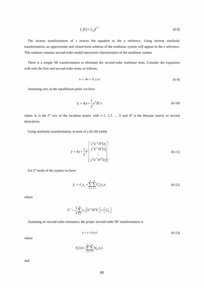
80

0( ) j t

j jz t z e

= (6-8)

The inverse transformation of z returns the equation to the y reference. Using inverse similarity

transformation, an approximate and closed-form solution of the nonlinear system will appear in the x reference.

This solution contains second-order modal interaction characteristics of the nonlinear system.

There is a simple NF transformation to eliminate the second-order nonlinear term. Consider the expansion

with only the first and second-order terms as follows;

2 ( )x Ax F x= + (6-9)

Assuming zero as the equilibrium point, we have

1

2

T i

i ix A x x H x= + (6-10)

where Ai is the ith row of the Jacobian matrix with i=1, 2,3, … N and Hi is the Hessian matrix of second

derivatives.

Using similarity transformation, in term of y (6-10) yields

1

21

2

T T

T T

T T N

y U H Uy

y U H Uyy y V

y U H Uy

= +

(6-11)

For jth mode of the system we have

1 1

N Nj

j j j kl k l

k l

y y C y y= =

= + (6-12)

where

1

1

2

Nj T l j

jl kl

k

C v U H U C=

= =

Assuming no second-order resonance, the proper second-order NF transformation is

2 ( )y z h z= + (6-13)

where

2 2

1 1

( )N N

j j

kl k l

k l

h z h z z= =

=

and

81

2

j

j kl

kl

k l j

Ch

=

+ −

Using the transformation (6-13), (6-12) can be represented in the NF space as

3( )j j jz z O z= + (6-14)

Neglecting high order terms of O(z3), the linear equation in (6-14) is solvable and has a solution identical to

(6-8). The approximate solution in Jordan space reference is;

( )

0 2 0 0

1 1

( ) i k l

N Nt tj

j j kl k l

k l

y t z e h z z e +

= =

= + (6-15)

Using the inverse similarity transformation, an approximated solution in physical space reference is given by

( )

0 2 0 0

1 1 1 1

( ) j k l

N N N Nt tj

i ij j ij kl k l

j j k l

x t u z e u h z z e +

= = = =

= +

(6-16)

Initial conditions are obtained using equations y0=Vx0 and z0 = y0 - h2 (z0). In the second equation, initial

conditions are obtained using numerical solution algorithms. Equations (6-15) and (6-16) give us the ability to

calculate the contribution of modes of oscillation to the system states. They allow direct comparison between

linear and nonlinear analysis including the second-order interactions. Nonlinear effects are exhibited in the NF

solution both in the linear part in the first terms of (6-16), and the second order interactions nonlinear part in the

second terms of (6-16).

This solution can be transformed back to the Jordan form as expressed in (6-17),

( )

0 2 0 0

1 1

( ) i k l

N Nt tj

j j kl k l

k l

y t z e h z z e +

= =

= + (6-17)

In (6-17), the first term represents the individual modes of the system, while the second term shows the system

second-order modal interaction. The ratio of the second term magnitude to the first term can be used to express

the impact of the second order modal interaction of the system as expressed in (6-18),

2 0 0

1 1

0

N Nj

kl k l

k l

j

j

h z z

Iz

= ==

(6-18)

Hereafter, Ij is called the index of nonlinearity. This index approximates the nonlinear characteristics, besides

the second-order modal interaction of the system.

Equations (6-18) and (6-9) show that the index can be excited by three main factors as presented below:

1. The Initial conditions (the size of zk0zl0)

2. A large value of Cjkl will cause a large value in hj

2kl

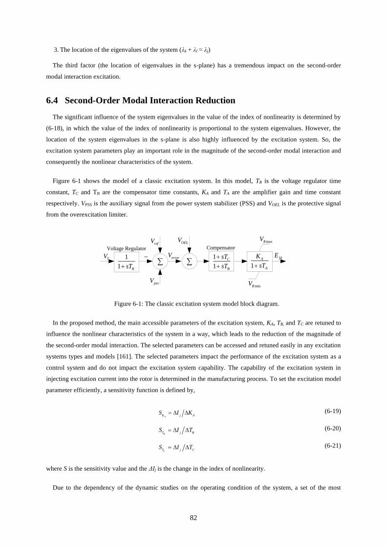
82

3. The location of the eigenvalues of the system (λk + λl ≈ λj)

The third factor (the location of eigenvalues in the s-plane) has a tremendous impact on the second-order

modal interaction excitation.

6.4 Second-Order Modal Interaction Reduction

The significant influence of the system eigenvalues in the value of the index of nonlinearity is determined by

(6-18), in which the value of the index of nonlinearity is proportional to the system eigenvalues. However, the

location of the system eigenvalues in the s-plane is also highly influenced by the excitation system. So, the

excitation system parameters play an important role in the magnitude of the second-order modal interaction and

consequently the nonlinear characteristics of the system.

Figure 6-1 shows the model of a classic excitation system. In this model, TR is the voltage regulator time

constant, TC and TB are the compensator time constants, KA and TA are the amplifier gain and time constant

respectively. VPSS is the auxiliary signal from the power system stabilizer (PSS) and VOEL is the protective signal

from the overexcitation limiter.

∑ 1

1 RsT+

1

1

C

B

sT

sT

+

+ 1

A

A

K

sT+

TV

refV

fdE−

minRV

maxRV

Voltage Regulator Compensator

∑

OELV

errorV

pssV

Figure 6-1: The classic excitation system model block diagram.

In the proposed method, the main accessible parameters of the excitation system, KA, TB, and TC are retuned to

influence the nonlinear characteristics of the system in a way, which leads to the reduction of the magnitude of

the second-order modal interaction. The selected parameters can be accessed and retuned easily in any excitation

systems types and models [161]. The selected parameters impact the performance of the excitation system as a

control system and do not impact the excitation system capability. The capability of the excitation system in

injecting excitation current into the rotor is determined in the manufacturing process. To set the excitation model

parameter efficiently, a sensitivity function is defined by,

AK j A

S I K= (6-19)

BT j B

S I T= (6-20)

CT j C

S I T= (6-21)

where S is the sensitivity value and the ΔIj is the change in the index of nonlinearity.

Due to the dependency of the dynamic studies on the operating condition of the system, a set of the most

83

probable operating scenarios must be considered. Figure 6-2 shows the algorithm of the proposed method. In the

first step, the rotor angle stability studies are performed, and if the system is stable, the next scenario will be

implemented. In the case of instability, the participation factor analysis is performed, and the speed and the rotor

angle related modes are identified. The proposed index of nonlinearity is then calculated for these modes and the

mode with the maximum index of nonlinearity is considered as Ijmax. In this step, a threshold value Ij

Threshold is set.

If Ijmax < Ij

Threshold, this mode will be neglected because of its linear behaviour; otherwise, it will be highly

nonlinear.

Increase

KA, TB, TC

System stable?

Perform participation factor analysis

Consider speed and angle related modes

Calculate Ij for each modes

IjMax

> IjThreshold ?

Calculate

SKA, STB, STC

Reduce

KA, TB, TC

Calculate and output Ij

Start

EndYes

No

PositiveNegative

Consider a mode with max Ij

Yes

No

Consider a specific operating condition

Figure 6-2: Flowchart of the proposed method.

The approach presented in Figure 6-2, retunes the excitation system parameters in an offline mode to reduce

the nonlinear characteristics of these modes. In the algorithm, the excitation parameters are increased gradually

to reach the lowest possible index of nonlinearity. The step is 2%. The criteria for the parameters selection are to

be within the acceptable range of the parameters indicated by the excitation system manufacturer. The algorithm

should be implemented for a selected operating condition which is identified as the most probable operating

condition by the network service provider (NSP). If the most probable operating condition is changed due to

significant network development, the algorithm should be re-run considering the new operating condition.

The most probable operating condition is normally labelled as the system's normal operating condition by

NSP. NSP network is normally expected to be operated in system normal operating conditions unless a

contingency or planned outage changes the operating condition of the network.

84

A proper exciter system design is achieved by calculating the sensitivity of the index of nonlinearity to each

parameter as expressed in (6-19), (6-20) and (6-21). If the sensitivity of a parameter is positive, the value of that

parameter is decreased by 2% and the index of nonlinearity recalculated and the algorithm enters another

iteration to see if the stable excitation system parameters are achieved. If the sensitivity of a parameter is

negative, the value of the parameter is increased by 2%. The new stable excitation system parameters are the

new tuning parameters.

6.5 Method Evaluation

The developed method is applied to a two-area, four generator test system taken from [12], which is modified

to consider different operating conditions according to [127]. The details of the considered two-area four

generator test system are presented in the appendix. These two areas are connected through two parallel

transmission lines. Each transmission line transfers 400 MW of active power. Figure 6-3 shows a single-line

diagram of the test system. For this study, all generators are modelled by the two-axis model and equipped with

an exciter [17], and the nominal apparent power for each generator is assumed to be 900 MVA. The output

operating voltage of each generator is 20 kV. The loads are modelled as constant impedances with no dynamics;

moreover, the generators are equipped with the excitation system. As a disturbance, the generation outage at

GEN4 is considered for 300 milliseconds. The simulation is carried out using DIgSILENT PowerFactory with 5

milliseconds simulation time step.

Area 1 Area 2

G1

G2

G3

G4

C1 C2L1 L2

1 25 6

4 3

Figure 6-3: Single line diagram of the test system.

First, the linear and the nonlinear characteristics of the test system are investigated using a time-domain

simulation and then the second-order modal interaction of the system is reduced using the new parameters for the

excitation system model.

6.5.1 Linear and Nonlinear Characteristics of the System

The behaviour of the linear and the nonlinear model of the test system after the disturbance are presented in

Figure 6-4. In Figure 6-4, after the outage clearance, the rotor angles of the GEN1 and GEN3 rise significantly

when using the nonlinear system model, but when using the linear system model, they can follow a stable route

towards their initial value. This significant difference between the nonlinear and linear modelling of the system

arises from the influence of the second-order modal interaction on the nonlinear modelling.

85

Figure 6-4: Rotor angle of the generators after the disturbance, (a) nonlinear system, (b) linear system.

A comparison between the results provided in Figure 6-4 indicated the significance of considering nonlinear

terms in the transient stability assessment of a power system. In Figure 6-4 (a) the test system nonlinear model

assessment shows that the disturbance causes transient instability while the same test system linear model

assessment in Figure 6-4 (b) shows that the system is stable in the presence of the same disturbance.

Additionally, it can be concluded that if the nonlinear characteristic of the nonlinear test system is reduced and

the system becomes more linear, the system behaviour in the presence of the disturbance will move from Figure

6-4 (a) to Figure 6-4 (b) and the test system transient stability will improve.

To determine the modes which are responsible for the second-order modal interaction in the nonlinear system,

a participation factor analysis is used. The participation factor analysis indicates the highest participation modes

in both the speed and the rotor angle of the generators. Table 6-1 represents the results of the participation factor

analysis for the 3 modes with the highest values of participation factors. These three modes are selected because

they were the best candidates to study the modal interaction between the generating units as all non-slack

generators were significantly participating to maintain the stability of these modes.

Table 6-1: The participation of each generator in electromechanical modes of the test system

Mode # Eigenvalue GEN1 GEN2 GEN3

1 -0.68 ± j6.68 0.25 0.60 0.47

2 -0.67 ± j6.65 0.59 0.35 0.14

3 -0.10 ± j3.24 0.27 0.033 0.49

The results from Table 6-1 show that for the third mode, GEN1 and GEN3 have the highest participation

factor while the participation factor of GEN2 is very small; so, mode 3 is originally generated from the

interaction between GEN1 and GEN3. To verify this, the proposed index of nonlinearity is also used to indicate

the nonlinear characteristics of the system with regards to the presented modes in Table 6-1. Table 6-2 shows the

value of the index of nonlinearity considering the mentioned electromechanical modes.

Table 6-2: The index of nonlinearity for the selected electromechanical modes

0 0.5 1 1.5 2 2.5 3-100

0

100

200

300

Time (Second)

Ro

tor

An

gle

(d

egre

e)

(a)

0 0.5 1 1.5 2 2.5 3-100

0

100

200

300

Time (Second)

Ro

tor

An

gle

(d

egre

e)

(b)

GEN1

GEN2

GEN3

86

jI 0jz Eigenvalue Mode#

0.05 1.70 -0.68 ± j6.68 1

0.05 2.07 -0.67 ± j6.65 2

0.72 2.09 -0.10 ± j3.24 3

The results from Table 6-2 verify the significant role of mode 3 in the magnitude of the second-order modal

interaction in the system; since mode 3 has the highest value of the index on nonlinearity. In other words, the

second-order modal interaction between GEN1 and GEN3 increases the nonlinear characteristics of the system.

6.5.2 Reduction in the Magnitude of the Second-order Modal Interaction

To reduce the magnitude of the second-order modal interaction of the test system, the proposed approach is

used to redesign the excitation system model parameters. In the first step, the sensitivity of each excitation

system model parameter to the index of nonlinearity using (6-19), (6-20), and (6-21) is calculated. If the

sensitivity of a parameter is positive, the value of that parameter is decreased, and in case of a negative

sensitivity, it will be increased. The magnitude of the change of a parameter is dependent on the sensitivity

magnitude. The most sensitive parameter will be the most impacted by the changes.

Table 6-3 show the selected sets of the excitation system model parameter tuning regarding reducing the

magnitude of the second-order modal interaction. In Table 6-3, four sets of excitation system model parameters

are selected among more than 30 sets of parameters, because they clearly show the gradual decrease in the value

of the nonlinearity index. Additionally, Table 6-3 shows the sensitivity of the parameters to the index on

nonlinearity for GEN1 and GEN3 and the value of the index of the nonlinearity of the system after implementing

the new parameters on the excitation system model. The sensitivity function of the first to third sets is calculated

against the fourth set because the fourth set is stable.

Table 6-3: Exciter system parameter along with their sensitivity and index of nonlinearity in four excitation

system model parameters setting

Set# GEN# AK BT

CT AKS

BTS CTS jI

Set I 1 220 8 2 -0.0008 0.025 -0.10

0.46 3 210 9 1.5 -0.0000 0.002 -0.10

Set II 1 240 7 3 -0.0005 0.019 -0.04

0.33 3 210 9 2.5 0.0000 0.000 -0.00

Set III 1 250 6 4 -0.0003 0.016 -0.02

0.27 3 210 9 3 0.0001 -0.002 0.00

Set IV 1 250 5.5 5 - - -

0.24 3 205 10 3 - - -

In this test system and the considered operating scenario, GEN1 and GEN3 are responsible for the magnitude

of the second-order modal interaction. As a result, the excitation system parameters of these two generators are

considered for retuning. Figure 6-5 up to Figure 6-8 shows the rotor angles of test system generators for each set

of the excitation system parameters.

87

Figure 6-5: Rotor angle of the generators for the exciter system parameter set I.

Figure 6-6: Rotor angle of the generators for the exciter system parameter set II.

0 0.5 1 1.5 2 2.5 3-100

-50

0

50

100

150

200

250

300

Time (Second)

Ro

tor

An

gle

(d

egre

e)

Set I

GEN1

GEN2

GEN3

0 0.5 1 1.5 2 2.5 3-100

-50

0

50

100

150

200

250

300

Time (Second)

Ro

tor

An

gle

(d

egre

e)

Set II

GEN1

GEN2

GEN3

88

Figure 6-7: Rotor angle of the generators for the exciter system parameter set III.

Figure 6-8: Rotor angle of the generators for the exciter system parameter set IV.

The time-domain simulation results of the rotor angles of the test system generators presented in Figure 6-5 up

to Figure 6-8 show that changes in the excitation system model parameters using the proposed method

significantly influence the characteristics of the system by reducing the magnitude of the second-order modal

interaction of the system. As is evident from Figure 6-5 up to Figure 6-8, as the index of nonlinearity reduces

from the set I to set IV, the nonlinear characteristic of the system reduces. In addition to the reduction of the

nonlinearity, the transformation in the nonlinear test system behaviour in the presence of the disturbance from

Figure 6-5 up to Figure 6-8 shows that as the nonlinear behaviour reduces, the transient stability of the nonlinear

test system improves.

0 0.5 1 1.5 2 2.5 3-100

-50

0

50

100

150

200

250

300

Time (Second)

Ro

tor

An

gle

(d

egre

e)

Set III

GEN1

GEN2

GEN3

0 0.5 1 1.5 2 2.5 3-100

-50

0

50

100

150

200

250

300

Time (Second)

Ro

tor

An

gle

(d

egre

e)

Set IV

GEN1

GEN2

GEN3

89

6.5.3 Expansion in the Transient Stability Boundaries

A time-domain analysis is carried out to investigate the influence of the reduction in the magnitude of the

second-order modal interaction on the transient stability of the system. In this situation, considering the same

disturbance like that of the previous section, the rotor angle behaviour for four different generating operating

scenarios is simulated. Table 6-4 presents detailed information about the four selected operating scenarios.

Table 6-4: Generator output power (MW) at the selected operating scenarios

Scenario I II III IV

Case 1: conventional parameters 560 602 607 700

Case 2: new parameters 560 665 700 707

The studies are carried out for two cases with different excitation system model parameters. In case 1, the

excitation system parameter of the set I given in Table 6-4 is considered, in which the index of the nonlinearity

of the system is 0.46. In case 2, the exciter system parameters of set IV given in Table 6-4 are considered, in

which the index of the nonlinearity of the system is 0.24. Each scenario was obtained by changing the active

power output of GEN1 and GEN3. In this study, the active power transfer between Area 1 and Area 2 remains

constant; since the inter-area oscillation is heavily dependent on the power transfer between areas.

Case1: In this case, the time-domain simulation results for GEN1 and GEN3 equipped with the set I excitation

system model parameters after the disturbance are presented in Figures 6-9 and 6-10.


exciter system parameters.

The system can remain stable for scenarios I and II but after a 5MW increase in the output active power of

both GEN1 and GEN3 in scenario III, the system exceeds its transient stability boundary and becomes unstable.

0 0.5 1 1.5 2 2.5 3-100

-50

0

50

100

150

200

250

300

Time (Second)

Ro

tor

An

gle

(d

egre

e)

GEN1

560 MW

602 MW

607 MW700 MW

90

Figure 6-10: Rotor angle of GEN3 after the event for different active power output scenarios with

conventional exciter system parameters.

Case 2: In this case, GEN1 and GEN3 are equipped with the excitation system model parameters of set IV.

These parameters are redesigned to reduce the magnitude of the second-order modal interaction.


system parameters.

Figures 6-11 and 6-12 show that the transient stability boundary of the test system has been increased due to

the reduction of the index of nonlinearity by using the new set of excitation system parameters. In other words,

the transient stability margin of the system is improved by redesigning the exciter system parameters.

0 0.5 1 1.5 2 2.5 3-100

-50

0

50

100

150

200

250

300

Time (Second)

Ro

tor

An

gle

(d

egre

e)

GEN3

560 MW

602 MW

607 MW700 MW

0 0.5 1 1.5 2 2.5 3-100

-50

0

50

100

150

200

250

300

Time (Second)

Ro

tor

An

gle

(d

egre

e)

GEN1

560 MW

665 MW

700 MW

707 MW

91


system parameters.

For this test system, the transient stability boundary of a single generator is increased by about 100 MW. In

other words, by using the new set of excitation system parameters, the power generation and transfer capacity of

the system may increase by about 15%.

6.6 Case Study

The performance of the proposed method of reducing the magnitude of the second-order modal interaction and

improving transient stability of the system by reducing the nonlinear characteristics of the system has been

evaluated using the IEEE 39-bus New England system [98]. The New England test system presented in Figure 6-

13 includes 10 generators.

0 0.5 1 1.5 2 2.5 3-100

-50

0

50

100

150

200

250

300

Time (Second)

Ro

tor

An

gle

(d

egre

e)

GEN3

560 MW

665 MW

700 MW

707 MW

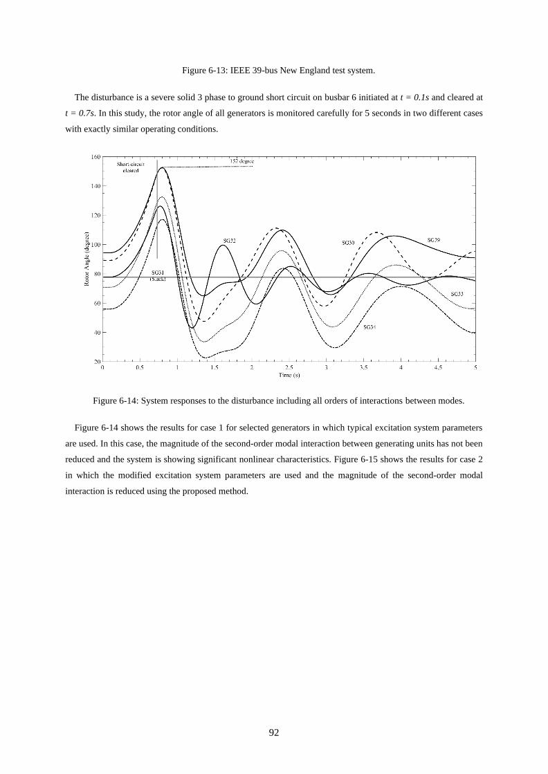
92

Figure 6-13: IEEE 39-bus New England test system.

The disturbance is a severe solid 3 phase to ground short circuit on busbar 6 initiated at t = 0.1s and cleared at

t = 0.7s. In this study, the rotor angle of all generators is monitored carefully for 5 seconds in two different cases

with exactly similar operating conditions.

Figure 6-14: System responses to the disturbance including all orders of interactions between modes.

Figure 6-14 shows the results for case 1 for selected generators in which typical excitation system parameters

are used. In this case, the magnitude of the second-order modal interaction between generating units has not been

reduced and the system is showing significant nonlinear characteristics. Figure 6-15 shows the results for case 2

in which the modified excitation system parameters are used and the magnitude of the second-order modal

interaction is reduced using the proposed method.

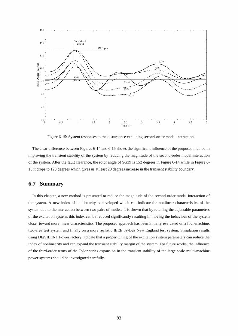
93

Figure 6-15: System responses to the disturbance excluding second-order modal interaction.

The clear difference between Figures 6-14 and 6-15 shows the significant influence of the proposed method in

improving the transient stability of the system by reducing the magnitude of the second-order modal interaction

of the system. After the fault clearance, the rotor angle of SG39 is 152 degrees in Figure 6-14 while in Figure 6-

15 it drops to 128 degrees which gives us at least 20 degrees increase in the transient stability boundary.

6.7 Summary

In this chapter, a new method is presented to reduce the magnitude of the second-order modal interaction of

the system. A new index of nonlinearity is developed which can indicate the nonlinear characteristics of the

system due to the interaction between two pairs of modes. It is shown that by retuning the adjustable parameters

of the excitation system, this index can be reduced significantly resulting in moving the behaviour of the system

closer toward more linear characteristics. The proposed approach has been initially evaluated on a four-machine,

two-area test system and finally on a more realistic IEEE 39-Bus New England test system. Simulation results

using DIgSILENT PowerFactory indicate that a proper tuning of the excitation system parameters can reduce the

index of nonlinearity and can expand the transient stability margin of the system. For future works, the influence

of the third-order terms of the Tylor series expansion in the transient stability of the large scale multi-machine

power systems should be investigated carefully.

94

Chapter 7 Conclusions and Future Works

7.1 Conclusions

In this thesis, the most economical and practical method to improve the characteristic of a power system in a

post-contingency operating condition have been developed.

The contributions of this thesis are as follows:

1) An optimal robust excitation system has been developed that improved the performance of the excitation

system during the emergency condition by being robust against the uncertainty of the excitation system

parameters;

2) A new OEL model is developed that improves the capability of the synchronous generator in supplying

reactive power longer to the grid in an emergency condition utilising the full thermal rating capability of

the rotor;

3) A novel method has been developed that can track the kinetic energy flow throughput the grid by

monitoring the propagated accelerating energy in the system. This method will indicate the amount of

stored energy in the system that may lead to transient instability;

4) A simple method has been introduced that can easily improve the transient stability of the system by

retuning the excitation system parameters in the system and reducing the nonlinear characteristic of the

network.

In Chapter 3, a new optimal robust IEEE ST1A excitation system controller is presented, which is robust to

the uncertainty in one or more of its parameters. Despite the complex mathematics behind the method, it can be

implemented simply and straightforwardly, even though the uncertainties in the model parameters exist. This

optimal approach has transferred the robust controller problem to an optimal control problem, while at the same

time, it has preserved the robustness of the excitation system. The influences of uncertainty in the values of KA,

with and without the design of the robust excitation system controller have been investigated for a single

machine test system. The simulation results from the dynamic stability simulation have demonstrated that the

designed robust excitation system controller is capable of being robust to the uncertainty in the parameters of an

excitation system controller. For the IEEE 39 bus system, the simulation results show that when the KA, TB and

TC values of the IEEE ST1A excitation system controller are changed to −20% of their nominal values, the

system becomes unstable although the system was stable when other values (within the upper and lower limit)

were used. However, when the designed optimal robust IEEE ST1A excitation system controller has been

applied, the system has become robust to the uncertainties in the parameters of the excitation system controller.

Using the proposed robust controller, the power system will not have any variation in its stability irrespective of

the values of the parameters within the boundary of the uncertainties.

In Chapter 4, a new method is proposed for the determination of the timing for OEL activation, which is

developed based on available generator rotor thermal capacity. The performance of the proposed method is

validated using two test systems. Using the single-machine test system, the simulation result shows that the

proposed OEL method can efficiently utilize the thermal capacity of the rotor and inject more reactive power

95

into the system in comparison with that from a conventional OEL equipped generators. The performance of the

proposed method is further validated using the Nordic power system demonstrating its effectiveness in extending

the amount of reactive power that can be supplied in a multi-machine network resulting in improved voltage

stability of the system. The results from the Nordic power system show that all generators participate in

supplying the reactive power after a severe disturbance; the conventional OEL equipped machines to participate

based on their electrical distance from the incident location, while the thermal-based OEL equipped units to

participate by considering their thermal capacity in addition to their distance from the disturbance. The generator

owners may be able to be persuaded to allow more use of the available reactive power contributions of the

generators to improve the power system performance and the voltage stability if incentives are provided through

the provision of ancillary and emergency control services in the electric power market. A system protection

scheme (SPS) using the operational data from a SCADA system can be used to identify the location and the

timing of the impending voltage instability by observing the sudden increase of generator reactive power outputs

and the reduction of voltages in the area of disturbance. The benefit of the proposed thermal-based OEL system

is to increase the time for such an SPS to function, by increasing the time so that enough reactive power can be

injected into the grid. This will provide the SPS more time to determine the best countermeasure that can be

effective to mitigate the emergency condition.

In Chapter 5, a new algorithm to detect transient instability is presented. This algorithm measures the

accelerating energy in two different stages. In the first stage, the accelerating energy created during the

disturbance is calculated. This accelerating energy is then called primary accelerating energy. In the next stage,

as the wave of energy passes through the grid it causes voltage drops in load busbars, which results in the

reductions in the load demands at the specific busbars, the reductions in the load demands add up to the existing

primary accelerating energy causing a secondary accelerating energy that keeps increasing as the wave of energy

passes through load busbars resulting in much longer transient stability or even transient instability. Finally, the

real-time determination of the propagated accelerating energy can be used as an indicator to detect transient

instability.

In Chapter 6, a new method is presented to reduce the second-order modal interaction of the system. A new

index of nonlinearity is developed which can indicate the nonlinear characteristics of the system due to the

interaction between the two pairs of modes. It is shown, that by retuning the adjustable parameters of the

excitation system, this index can be reduced significantly resulting in moving the behaviour of the system closer

toward more linear characteristics. The proposed approach has been initially evaluated on a four-machine, two-

area test system and finally on a more realistic IEEE 39-Bus New England test system. Simulation results using

DIgSILENT PowerFactory indicate that a proper tuning of the excitation system parameters can reduce the index

of nonlinearity and can expand the transient stability margin of the system.

7.2 Future Works

The concept of the emergency control of a power grid that has been developed in this thesis can be developed

further.

The key factors of being practical and efficient in addition to economic consideration should always be the

96

main aims of any emergency control scheme. In communication with the Australian transmission system

operator, it was recommended that the solutions that can be implemented must be cost-effective in its approach.

Any economical solution to the emergency control issue is very attractive for the transmission system operators.

The work that has been carried out in this thesis can be extended and continued in the following recommended

areas:

1) Similar to the excitation controller, the prime mover and governor can be developed to be robust to any

uncertainty in their parameters. The approach can be adapted from the design process introduced in

Chapter 3 for the excitation controller. An optimal robust prime mover and governor can improve the

capability of the system in dealing with the frequency related contingency, specifically when the power

grid is being operated close to its limits. In addition to the excitation system, the prime mover and the

governor of the synchronous machine, other synchronous machine controllers and protection systems

such as the overexcitation limiter, the under excitation limiter, the rate change of frequency protection

system and the passive and active islanding protection systems can be developed to be robust to the

variations in the synchronous generator parameters or variations in the operating condition of the

network.

2) The proposed OEL method in Chapter 4 extends the capability of the generator in supplying more

reactive power in a post-contingency operating condition. Considering this capability, the under-

voltage load shedding schemes should be developed to allow more time delays in the operation of the

curtailment scheme. Corrective actions can also be implemented in the provided extra time to avoid the

activation of load-shedding schemes.

3) The rotor thermal capability concept developed in Chapter 4 can be used for any overcurrent protection

system. Using this developed method, the thermal capability of any element can be efficiently used,

and the element can operate in the overloaded condition for a longer period without being damaged.

This method helps the operators to use the full capability of any element in the overloaded condition

without damaging the element. This improvement can also be obtained by considering a direct

temperature measurement in the overloaded elements. Thermography based measurement methods can

be utilized to directly measure the temperature in an overloaded element without needing to have direct

contact. This temperature measurement can be used to avoid damages to any overloaded elements.

4) Transient stability detection has always been a challenging concept in power system security. Using

the proposed method in Chapter 5, the propagated accelerating energy in a power system can be

measured as a wave of energy spreading throughout the network in time, pattern recognition

algorithms can be explored to predict the time that the system will reach the transient instability limit.

The pattern recognition methods can be trained offline for a specific large-scale power system and then

implemented in real-time to estimate the time in which the transient instability is imminent. This time

can be used for the activation of the countermeasure.

5) The concept of the propagated accelerating energy can be used to determine the effectiveness of a

97

transient stability countermeasure. The countermeasure can be implemented and the amount of energy

dissipation after the implementation can be measured and the effectiveness of the countermeasure will

be ranked. Moreover, this concept can be used to locate the most effective location for the

countermeasure to be installed.

6) As a countermeasure to avoid transient stability in a large power system, storage systems can be

installed in the load zone substations to reduce the SAE caused by loads, the size of the storage

systems can be selected based of the relationship between the voltage magnitude of the load and the

active power load demand as indicated in Chapter 5. Based on the concept of the propagated

accelerating energy, the time to actuate the storage systems as a countermeasure can be obtained

through recognizing the pattern of the increasing PAE and SAE.

7) The investigation of the influence of the voltage magnitudes of the busbars to the accelerating speed of

the propagated energy needs to be investigated. The investigations in Chapter 5 indicated that the

dependency between the active and reactive power demand in the load substation to the voltage

magnitude of the load determines the speed of the wave of energy passing throughout the grid. For

loads that are highly sensitive to the voltage magnitude, the wave of energy will spread much faster

than that from the less sensitive loads. The speed of the propagated accelerating energy spreading out

through the system can be studied and the critical factors can be identified. This will lead to the

identification of the most critical parameters of the system in transient stability and can be used in

improving the transient stability of the system.

8) In addition to the second-order modal interaction investigated in Chapter 6, a third-order modal

interaction between the different modes of the system can be investigated as well. To study the

influence of the third-order interaction between the system modes, the use of a third-order Taylor

series expansion terms needs to be studied.

98

References

[1] D. Sutanto and W. R. Lachs, “A fresh approach to improve power system security,” in 2004

International Conference on Power System Technology, 2004. PowerCon 2004., 2004, vol. 1, pp. 975–

980.

[2] W. R. Lachs, “A new horizon for system protection schemes,” IEEE Trans. Power Syst., vol. 18, no. 1,

pp. 334–338, 2003.

[3] C.-C. Liu, J. Jung, G. T. Heydt, V. Vittal, and A. G. Phadke, “The strategic power infrastructure defense

(SPID) system. A conceptual design,” IEEE Control Syst. Mag., vol. 20, no. 4, pp. 40–52, 2000.

[4] W. R. Lachs, “Area-wide system protection scheme against extreme contingencies,” Proc. IEEE, vol. 93,

no. 5, pp. 1004–1027, 2005.

[5] A. Muir and J. Lopatto, “Final report on the August 14, 2003 blackout in the United States and Canada:

causes and recommendations,” 2004.

[6] Y. V Makarov, V. I. Reshetov, A. Stroev, and I. Voropai, “Blackout prevention in the united states,

Europe, and Russia,” Proc. IEEE, vol. 93, no. 11, pp. 1942–1955, 2005.

[7] G. A. Maas, M. Bial, and J. Fijalkowski, “Final report-system disturbance on 4 november 2006,” Union

Coord. Transm. Electr. Eur. Tech. Rep, 2007.

[8] N. I. Voropai et al., “Smart technologies in emergency control of Russia’s unified energy system,” IEEE

Trans. Smart Grid, vol. 4, no. 3, pp. 1732–1740, 2013.

[9] Y. V Makarov, N. I. Voropai, and D. N. Efimov, “Complex emergency control system against blackouts

in Russia,” in 2008 IEEE Power and Energy Society General Meeting-Conversion and Delivery of

Electrical Energy in the 21st Century, 2008, pp. 1–8.

[10] D. Sutanto and W. R. Lachs, “Control measures for improving power system reliability,” in 1991

International Conference on Advances in Power System Control, Operation and Management,

APSCOM-91., 1991, pp. 751–756 vol.2.

[11] S. R. Islam, K. M. Muttaqi, and D. Sutanto, “Multi-agent receding horizon control with neighbour-to-

neighbour communication for prevention of voltage collapse in a multi-area power system,” IET Gener.

Transm. Distrib., vol. 8, no. 9, pp. 1604–1615, 2014.

[12] H. Lomei, D. Sutanto, K. M. Muttaqi, and M. Assili, “A new approach to reduce the non-linear

characteristics of a stressed power system by using the normal form technique in the control design of

the excitation system,” in 2015 IEEE Industry Applications Society Annual Meeting, 2015, pp. 1–6.

[13] F. P. Demello and C. Concordia, “Concepts of synchronous machine stability as affected by excitation

control,” IEEE Trans. power Appar. Syst., vol. 88, no. 4, pp. 316–329, 1969.

[14] V. Vittal and M. Khammash, “Decentralized power system stabilizer design using linear parameter

varying approach,” IEEE Trans. Power Syst., vol. 19, no. 4, pp. 1951–1960, Nov. 2004.

[15] N. Jiang and H. Chiang, “A Two-Time Scale Dynamic Correction Method for Fifth-Order Generator

Model Undergoing Large Disturbances,” IEEE Trans. Power Syst., vol. 31, no. 5, pp. 3616–3623, 2016.

[16] T. K. Roy, M. A. Mahmud, and A. M. T. Oo, “Robust Adaptive Backstepping Excitation Controller

Design for Higher-Order Models of Synchronous Generators in Multimachine Power Systems,” IEEE

Trans. Power Syst., vol. 34, no. 1, pp. 40–51, Jan. 2019.

[17] P. Kundur, N. J. Balu, and M. G. Lauby, Power system stability and control, vol. 7. McGraw-hill New

99

York, 1994.

[18] R. Majumder, B. Chaudhuri, H. El-Zobaidi, B. C. Pal, and I. M. Jaimoukha, “LMI approach to

normalised H8 loop-shaping design of power system damping controllers,” IEE Proceedings-

Generation, Transm. Distrib., vol. 152, no. 6, pp. 952–960, 2005.

[19] M. J. Hossain, H. R. Pota, V. A. Ugrinovskii, and R. A. Ramos, “Voltage mode stabilisation in power

systems with dynamic loads,” Int. J. Electr. Power Energy Syst., vol. 32, no. 9, pp. 911–920, 2010.

[20] P. Kundur, M. Klein, G. J. Rogers, and M. S. Zywno, “Application of power system stabilizers for

enhancement of overall system stability,” IEEE Trans. Power Syst., vol. 4, no. 2, pp. 614–626, 1989.

[21] S. Cheng, R. Zhou, and L. Guan, “An on-line self-learning power system stabilizer using a neural

network method,” IEEE Trans. power Syst., vol. 12, no. 2, pp. 926–931, 1997.

[22] E. V Larsen and D. A. Swann, “Applying power system stabilizers Part III: Practical considerations,”

IEEE Trans. power Appar. Syst., no. 6, pp. 3034–3046, 1981.

[23] A. Feliachi, X. Zhang, and C. S. Sims, “Power system stabilizers design using optimal reduced order

models. I. Model reduction,” IEEE Trans. Power Syst., vol. 3, no. 4, pp. 1670–1675, 1988.

[24] J. Y. Fan, T. H. Ortmeyer, and R. Mukundan, “Power system stability improvement with multivariable

self-tuning control,” IEEE Trans. power Syst., vol. 5, no. 1, pp. 227–234, 1990.

[25] G. Gurrala and I. Sen, “Power system stabilizers design for interconnected power systems,” IEEE Trans.

Power Syst., vol. 25, no. 2, pp. 1042–1051, 2010.

[26] Y. Yu, K. Vongsuriya, and L. N. Wedman, “Application of an optimal control theory to a power

system,” IEEE Trans. Power Appar. Syst., no. 1, pp. 55–62, 1970.

[27] Q. Lu, S. Mei, W. Hu, F. F. Wu, Y. Ni, and T. Shen, “Nonlinear decentralized disturbance attenuation

excitation control via new recursive design for multi-machine power systems,” IEEE Trans. Power Syst.,

vol. 16, no. 4, pp. 729–736, 2001.

[28] A. Colbia-Vega, J. de Leon-Morales, L. Fridman, O. Salas-Pena, and M. T. Mata-Jiménez, “Robust

excitation control design using sliding-mode technique for multimachine power systems,” Electr. Power

Syst. Res., vol. 78, no. 9, pp. 1627–1634, 2008.

[29] Y. Liu, T. Chen, C. Li, Y. Wang, and B. Chu, “Energy-Based $ L_2 $ Disturbance Attenuation

Excitation Control of Differential Algebraic Power Systems,” IEEE Trans. Circuits Syst. II Express

Briefs, vol. 55, no. 10, pp. 1081–1085, 2008.

[30] P. Zhao, W. Yao, J. Wen, L. Jiang, S. Wang, and S. Cheng, “Improved synergetic excitation control for

transient stability enhancement and voltage regulation of power systems,” Int. J. Electr. Power Energy

Syst., vol. 68, pp. 44–51, 2015.

[31] H. E. Psillakis and A. T. Alexandridis, “A new excitation control for multimachine power systems. I:

Decentralized nonlinear adaptive control design and stability analysis,” Int. J. Control. Autom. Syst., vol.

3, no. 2, pp. 278–287, 2005.

[32] W. Yao, L. Jiang, J. Fang, J. Wen, and S. Cheng, “Decentralized nonlinear optimal predictive excitation

control for multi-machine power systems,” Int. J. Electr. Power Energy Syst., vol. 55, pp. 620–627,

2014.

[33] H. Liu, Z. Hu, and Y. Song, “Lyapunov-based decentralized excitation control for global asymptotic

stability and voltage regulation of multi-machine power systems,” IEEE Trans. Power Syst., vol. 27, no.

100

4, pp. 2262–2270, 2012.

[34] M. A. Mahmud, H. R. Pota, M. Aldeen, and M. J. Hossain, “Partial feedback linearizing excitation

controller for multimachine power systems to improve transient stability,” IEEE Trans. Power Syst., vol.

29, no. 2, pp. 561–571, 2014.

[35] D. Gan, Z. Qu, and H. Cai, “Multi machine power system excitation control design via theories of

feedback linearization control and nonlinear robust control,” Int. J. Syst. Sci., vol. 31, no. 4, pp. 519–527,

2000.

[36] G. Guo, Y. Wang, and D. J. Hill, “Nonlinear output stabilization control for multimachine power

systems,” IEEE Trans. Circuits Syst. I Fundam. Theory Appl., vol. 47, no. 1, pp. 46–53, 2000.

[37] C. A. King, J. W. Chapman, and M. D. Ilic, “Feedback linearizing excitation control on a full-scale

power system model,” IEEE Trans. Power Syst., vol. 9, no. 2, pp. 1102–1109, 1994.

[38] Y. Wang, G. Guo, and D. J. Hill, “Nonlinear decentralized coordinated control for multimachine power

systems,” in Proceedings 1995 International Conference on Energy Management and Power Delivery

EMPD’95, 1995, vol. 1, pp. 102–107.

[39] Y. Wang, D. J. Hill, R. H. Middleton, and L. Gao, “Transient stabilization of power systems with an

adaptive control law,” Automatica, vol. 30, no. 9, pp. 1409–1413, 1994.

[40] M. A. Mahmud, H. R. Pota, and M. J. Hossain, “Full-order nonlinear observer-based excitation

controller design for interconnected power systems via exact linearization approach,” Int. J. Electr.

Power Energy Syst., vol. 41, no. 1, pp. 54–62, 2012.

[41] M. A. Mahmud, “An alternative LQR-based excitation controller design for power systems to enhance

small-signal stability,” Int. J. Electr. Power Energy Syst., vol. 63, pp. 1–7, 2014.

[42] T. K. Roy, M. A. Mahmud, W. Shen, and A. M. T. Oo, “Nonlinear Adaptive Excitation Controller

Design for Multimachine Power Systems With Unknown Stability Sensitive Parameters,” IEEE Trans.

Control Syst. Technol., vol. 25, no. 6, pp. 2060–2072, Nov. 2017.

[43] J. Li, Y. Liu, C. Li, and B. Chu, “Passivity-based nonlinear excitation control of power systems with

structure matrix reassignment,” Information, vol. 4, no. 3, pp. 342–350, 2013.

[44] R. Goldoost-Soloot, Y. Mishra, and G. Ledwich, “Design of a nonlinear excitation controller using

inverse filtering for transient stability enhancement,” in 2014 IEEE PES General Meeting| Conference &

Exposition, 2014, pp. 1–5.

[45] S. S. Majidabad, H. T. Shandiz, and A. Hajizadeh, “Nonlinear fractional-order power system stabilizer

for multi-machine power systems based on sliding mode technique,” Int. J. Robust Nonlinear Control,

vol. 25, no. 10, pp. 1548–1568, 2015.

[46] X. Liu and Y. Han, “Decentralized multi-machine power system excitation control using continuous

higher-order sliding mode technique,” Int. J. Electr. Power Energy Syst., vol. 82, pp. 76–86, 2016.

[47] M. Mohamed, X.-G. Yan, S. K. Spurgeon, and B. Jiang, “Robust sliding-mode observers for large-scale

systems with application to a multimachine power system,” IET Control Theory Appl., vol. 11, no. 8, pp.

1307–1315, 2016.

[48] T. F. Orchi, T. K. Roy, M. A. Mahmud, and A. M. T. Oo, “Feedback Linearizing Model Predictive

Excitation Controller Design for Multimachine Power Systems,” IEEE Access, vol. 6, pp. 2310–2319,

2018.

101

[49] R. A. Ramos, L. F. C. Alberto, and N. G. Bretas, “A new methodology for the coordinated design of

robust decentralized power system damping controllers,” IEEE Trans. Power Syst., vol. 19, no. 1, pp.

444–454, 2004.

[50] A. Pal, J. S. Thorp, S. S. Veda, and V. A. Centeno, “Applying a robust control technique to damp low

frequency oscillations in the WECC,” Int. J. Electr. Power Energy Syst., vol. 44, no. 1, pp. 638–645,

2013.

[51] S. Jain, F. Khorrami, and B. Fardanesh, “Adaptive nonlinear excitation control of power systems with

unknown interconnections,” IEEE Trans. Control Syst. Technol., vol. 2, no. 4, pp. 436–446, 1994.

[52] S. Jain and F. Khorrami, “Robust decentralized control of power systems utilizing only swing angle

measurements,” Int. J. Control, vol. 66, no. 4, pp. 581–602, 1997.

[53] Y. L. Tan and Y. Wang, “Nonlinear excitation and phase shifter controller for transient stability

enhancement of power systems using adaptive control law,” Int. J. Electr. Power Energy Syst., vol. 18,

no. 6, pp. 397–403, 1996.

[54] H. Jiang, J. F. Dorsey, Z. Qu, J. Bond, and J. M. McCalley, “Global robust adaptive control of power

systems,” IEE Proceedings-Generation, Transm. Distrib., vol. 141, no. 5, pp. 429–436, 1994.

[55] Y. Wang and D. J. Hill, “Robust nonlinear coordinated control of power systems,” Automatica, vol. 32,

no. 4, pp. 611–618, 1996.

[56] Y. Wang, L. Xie, D. J. Hill, and R. H. Middleton, “Robust nonlinear controller design for transient

stability enhancement of power systems,” in [1992] Proceedings of the 31st IEEE Conference on

Decision and Control, 1992, pp. 1117–1122.

[57] Y. Wang, G. Guo, and D. J. Hill, “Robust decentralized nonlinear controller design for multimachine

power systems,” Automatica, vol. 33, no. 9, pp. 1725–1733, 1997.

[58] Y. Wang, Y. L. Tan, and G. Guo, “Robust nonlinear coordinated generator excitation and SVC control

for power systems,” Int. J. Electr. Power Energy Syst., vol. 22, no. 3, pp. 187–195, 2000.

[59] Y. Wang, G. H. Zhang, and D. J. Hill, “Robust power system transient stability enhancement: A global

control approach,” IFAC Proc. Vol., vol. 37, no. 13, pp. 1045–1050, 2004.

[60] L. Cong, Y. Wang, and D. J. Hill, “Co-ordinated control design of generator excitation and SVC for

transient stability and voltage regulation enhancement of multi-machine power systems,” Int. J. Robust

Nonlinear Control IFAC-Affiliated J., vol. 14, no. 9–10, pp. 789–805, 2004.

[61] L. Cong, Y. Wang, and D. J. Hill, “Transient stability and voltage regulation enhancement via

coordinated control of generator excitation and SVC,” Int. J. Electr. Power Energy Syst., vol. 27, no. 2,

pp. 121–130, 2005.

[62] R. Yan, Z. Y. Dong, T. K. Saha, and R. Majumder, “Power system transient stability enhancement with

an adaptive control scheme using backstepping design,” in 2007 IEEE Power Engineering Society

General Meeting, 2007, pp. 1–8.

[63] R. Yan, Z. Dong, T. K. Saha, and R. Majumder, “A power system nonlinear adaptive decentralized

controller design,” Automatica, vol. 46, no. 2, pp. 330–336, 2010.

[64] I. Kanellakopoulos, P. V Kokotovic, and A. S. Morse, “Systematic design of adaptive controllers for

feedback linearizable systems,” in 1991 American Control Conference, 1991, pp. 649–654.

[65] M. Krstic, I. Kanellakopoulos, P. V Kokotovic, and others, Nonlinear and adaptive control design, vol.

102

222. Wiley New York, 1995.

[66] D. Karagiannis and A. Astolfi, “Nonlinear adaptive control of systems in feedback form: An alternative

to adaptive backstepping,” Syst. Control Lett., vol. 57, no. 9, pp. 733–739, 2008.

[67] K. Wang, H. Xin, D. Gan, and Y. Ni, “Non-linear robust adaptive excitation controller design in power

systems based on a new back-stepping method,” IET Control theory Appl., vol. 4, no. 12, pp. 2947–

2957, 2010.

[68] C. Sun, Z. Zhao, Y. Sun, and Q. Lu, “Design of nonlinear robust excitation control for multimachine

power systems,” IEE Proceedings-Generation, Transm. Distrib., vol. 143, no. 3, pp. 253–257, 1996.

[69] A. I. Zecevic, G. Neskovic, and D. D. Siljak, “Robust decentralized exciter control with linear

feedback,” IEEE Trans. Power Syst., vol. 19, no. 2, pp. 1096–1103, 2004.

[70] P. S. Rao and I. Sen, “Robust pole placement stabilizer design using linear matrix inequalities,” IEEE

Trans. Power Syst., vol. 15, no. 1, pp. 313–319, 2000.

[71] G. E. Boukarim, S. Wang, J. H. Chow, G. N. Taranto, and N. Martins, “A comparison of classical,

robust, and decentralized control designs for multiple power system stabilizers,” IEEE Trans. Power

Syst., vol. 15, no. 4, pp. 1287–1292, 2000.

[72] Y. L. Abdel-Magid and M. A. Abido, “Optimal multiobjective design of robust power system stabilizers

using genetic algorithms,” IEEE Trans. power Syst., vol. 18, no. 3, pp. 1125–1132, 2003.

[73] A. Hasanovic, A. Feliachi, N. B. Bhatt, and A. G. DeGroff, “Practical robust PSS design through

identification of low-order transfer functions,” IEEE Trans. Power Syst., vol. 19, no. 3, pp. 1492–1500,

2004.

[74] D. D. Siljak, D. M. Stipanovic, and A. I. Zecevic, “Robust decentralized turbine/governor control using

linear matrix inequalities,” IEEE Trans. Power Syst., vol. 17, no. 3, pp. 715–722, 2002.

[75] Q. Zhao and J. Jiang, “Robust SVC controller design for improving power system damping,” IEEE


[76] M. Parniani and M. R. Iravani, “Optimal robust control design of static VAR compensators,” IEE

Proceedings-Generation, Transm. Distrib., vol. 145, no. 3, pp. 301–307, 1998.

[77] Y. Wan, J. Zhao, and G. M. Dimirovski, “Robust adaptive control for a single-machine infinite-bus

power system with an SVC,” Control Eng. Pract., vol. 30, pp. 132–139, 2014.

[78] X. Yu, M. Khammash, and V. Vittal, “Robust design of a damping controller for static var compensators

in power systems,” IEEE Trans. Power Syst., vol. 16, no. 3, pp. 456–462, 2001.

[79] H. Liu, X. Xie, L. Wang, and Y. Han, “Optimal design of linear subsynchronous damping controllers for

stabilising torsional interactions under all possible operating conditions,” IET Gener. Transm. Distrib.,

vol. 9, no. 13, pp. 1652–1661, 2015.

[80] J. C. Agee et al., “Recommended Models for Overexcitation Limiting Devices,” IEEE Power Eng. Rev.,

vol. 15, no. 12, p. 38, 1995.

[81] C. D. Vournas, G. A. Manos, P. W. Sauer, and M. A. Pai, “Effect of overexcitation limiters on power

system long-term modeling,” IEEE Trans. Energy Convers., vol. 14, no. 4, pp. 1529–1536, 1999.

[82] C. A. Aumuller and T. K. Saha, “Investigating the impact of Powerformer on voltage stability by

dynamic simulation,” IEEE Trans. Power Syst., vol. 18, no. 3, pp. 1142–1148, 2003.

[83] C. W. Taylor, Criteria and countermeasures for voltage collapse. CIGRE, 1995.

103

[84] C. J. Parker, Power System Voltage Stability: Analytical Approaches to Modelling, Mid-term Simulation

and Corrective Action. University of New South Wales, 1997.

[85] M. Shimomura, Y. Xia, M. Wakabayashi, and J. Paserba, “A new advanced over excitation limiter for

enhancing the voltage stability of power systems,” in 2001 IEEE Power Engineering Society Winter

Meeting. Conference Proceedings (Cat. No. 01CH37194), 2001, vol. 1, pp. 221–227.

[86] A. Murdoch, G. E. Boukarim, B. E. Gott, M. J. D’antonio, and R. A. Lawson, “Generator over excitation

capability and excitation system limiters,” in 2001 IEEE Power Engineering Society Winter Meeting.

Conference Proceedings (Cat. No. 01CH37194), 2001, vol. 1, pp. 215–220.

[87] Y. Kataoka and Y. Shinoda, “Voltage stability limit of electric power systems with generator reactive

power constraints considered,” IEEE Trans. Power Syst., vol. 20, no. 2, pp. 951–962, 2005.

[88] C. J. Parker, I. F. Morrison, and D. Sutanto, “Application of an optimisation method for determining the

reactive margin from voltage collapse in reactive power planning,” IEEE Trans. Power Syst., vol. 11, no.

3, pp. 1473–1481, 1996.

[89] O. A. Mousavi and R. Cherkaoui, “Maximum voltage stability margin problem with complementarity

constraints for multi-area power systems,” IEEE Trans. Power Syst., vol. 29, no. 6, pp. 2993–3002,

2014.

[90] D. Marujo, A. C. Z. De Souza, B. I. L. Lopes, M. V Santos, and K. L. Lo, “On Control Actions Effects

by Using $${$$\$rm QV$}$ $ Curves,” IEEE Trans. Power Syst., vol. 30, no. 3, pp. 1298–1305, 2015.

[91] H. Lomei, K. M. Muttaqi, and D. Sutanto, “A new method to determine the activation time of the

overexcitation limiter based on available generator rotor thermal capacity for improving long-term

voltage instability,” IEEE Trans. Power Syst., vol. 32, no. 3, pp. 1711–1720, 2017.

[92] A. Nasri, M. Ghandhari, and R. Eriksson, “Transient stability assessment of power systems in the

presence of shunt compensators using trajectory sensitivity analysis,” in 2013 IEEE Power Energy

Society General Meeting, 2013, pp. 1–5.

[93] P. Bhui and N. Senroy, “Real-Time Prediction and Control of Transient Stability Using Transient Energy

Function,” IEEE Trans. Power Syst., vol. 32, no. 2, pp. 923–934, Mar. 2017.

[94] A. A. Fouad, “Transient stability criteria,” in 1975 IEEE Conference on Decision and Control including

the 14th Symposium on Adaptive Processes, 1975, pp. 309–314.

[95] J. Shu, W. Xue, and W. Zheng, “A parallel transient stability simulation for power systems,” IEEE


[96] I. Nagel, L. Fabre, M. Pastre, F. ç ois Krummenacher, R. Cherkaoui, and M. Kayal, “High-speed power

system transient stability simulation using highly dedicated hardware,” IEEE Trans. Power Syst., vol. 28,

no. 4, pp. 4218–4227, 2013.

[97] Y. Li and Z. Yang, “Application of EOS-ELM with binary Jaya-based feature selection to real-time

transient stability assessment using PMU data,” IEEE Access, vol. 5, pp. 23092–23101, 2017.

[98] T. Athay, R. Podmore, and S. Virmani, “A practical method for the direct analysis of transient stability,”

IEEE Trans. Power Appar. Syst., no. 2, pp. 573–584, 1979.

[99] T. Odun-Ayo and M. L. Crow, “Structure-preserved power system transient stability using stochastic

energy functions,” IEEE Trans. Power Syst., vol. 27, no. 3, pp. 1450–1458, 2012.

[100] A. Vahidnia, G. Ledwich, E. Palmer, and A. Ghosh, “Wide-area control through aggregation of power

104

systems,” IET Gener. Transm. Distrib., vol. 9, no. 12, pp. 1292–1300, 2015.

[101] A. Vahidnia, G. Ledwich, and E. W. Palmer, “Transient stability improvement through wide-area

controlled SVCs,” IEEE Trans. Power Syst., vol. 31, no. 4, pp. 3082–3089, 2015.

[102] R. Goldoost-Soloot, Y. Mishra, and G. Ledwich, “Wide-area damping control for inter-area oscillations

using inverse filtering technique,” IET Gener. Transm. Distrib., vol. 9, no. 13, pp. 1534–1543, 2015.

[103] A. A. Fouad and S. E. Stanton, “Transient stability of a multi-machine power system Part I: Investigation

of system trajectories,” IEEE Trans. power Appar. Syst., no. 7, pp. 3408–3416, 1981.

[104] A. A. Fouad and S. E. Stanton, “Transient stability of a multi-machine power system. Part II: Critical

transient energy,” IEEE Trans. power Appar. Syst., no. 7, pp. 3417–3424, 1981.

[105] V. Vittal, “Power system transient stability using the critical energy of individual machines,” 1982.

[106] A. Michel, A. Fouad, and V. Vittal, “Power system transient stability using individual machine energy

functions,” IEEE Trans. Circuits Syst., vol. 30, no. 5, pp. 266–276, 1983.

[107] S. E. Stanton, “Assessment of the stability of a multimachine power system by the transient energy

margin,” 1982.

[108] S. E. Stanton and W. P. Dykas, “Analysis of a local transient control action by partial energy functions,”

IEEE Trans. Power Syst., vol. 4, no. 3, pp. 996–1002, 1989.

[109] S. E. Stanton, “Transient stability monitoring for electric power systems using a partial energy function,”


[110] S. E. Stanton, C. Slivinsky, K. Martin, and J. Nordstrom, “Application of phasor measurements and

partial energy analysis in stabilizing large disturbances,” IEEE Trans. Power Syst., vol. 10, no. 1, pp.

297–306, 1995.

[111] P. Rastgoufard, A. Yazdankhah, and R. A. Schlueter, “Multi-machine equal area based power system

transient stability measure,” IEEE Trans. power Syst., vol. 3, no. 1, pp. 188–196, 1988.

[112] M. H. Haque, “Further developments of the equal-area criterion for multimachine power systems,”

Electr. power Syst. Res., vol. 33, no. 3, pp. 175–183, 1995.

[113] R. Ando and S. Iwamoto, “Highly reliable transient stability solution method using energy function,”

Electr. Eng. Japan, vol. 108, no. 4, pp. 57–66, 1988.

[114] T. Tian, X. Kestelyn, O. Thomas, H. Amano, and A. R. Messina, “An accurate third-order normal form

approximation for power system nonlinear analysis,” IEEE Trans. Power Syst., vol. 33, no. 2, pp. 2128–

2139, 2017.

[115] N. Yorino, H. Sasaki, Y. Tamura, and R. Yokoyama, “A generalized analysis method of auto-parametric

resonances in power systems,” IEEE Trans. Power Syst., vol. 4, no. 3, pp. 1057–1064, 1989.

[116] Y. Tamura and N. Yorino, “Possibility of auto-& hetero-parametric resonances in power systems and

their relationship with long-term dynamics,” IEEE Trans. Power Syst., vol. 2, no. 4, pp. 890–896, 1987.

[117] V. Vittal, N. Bhatia, and A. A. Fouad, “Analysis of the inter-area mode phenomenon in power systems

following large disturbances,” IEEE Trans. Power Syst., vol. 6, no. 4, pp. 1515–1521, 1991.

[118] S. K. Starrett, W. Kliemann, V. Vittal, and A. A. Fouad, “Power system modal behavior: Significance of

second and third order nonlinear terms,” in Proc. North American Power Symp., Washington, DC, 1993,

pp. 241–255.

[119] A. A. Fouad, V. Vittal, W. Kliemann, S. K. Starrett, and C. M. Lin, “Analysis of stressed interconnected

105

power networks. Final report,” 1994.

[120] C.-M. Lin, V. Vittal, W. Kliemann, and A. A. Fouad, “Investigation of modal interaction and its effects

on control performance in stressed power systems using normal forms of vector fields,” IEEE Trans.

power Syst., vol. 11, no. 2, pp. 781–787, 1996.

[121] Y.-X. Ni, V. Vittal, W. Kliemann, and A. A. Fouad, “Nonlinear modal interaction in HVDC/AC power

systems with DC power modulation,” IEEE Trans. Power Syst., vol. 11, no. 4, pp. 2011–2017, 1996.

[122] J. Thapar, V. Vittal, W. Kliemann, and A. A. Fouad, “Application of the normal form of vector fields to

predict interarea separation in power systems,” IEEE Trans. Power Syst., vol. 12, no. 2, pp. 844–850,

1997.

[123] G. Jang, V. Vittal, and W. Kliemann, “Effect of nonlinear modal interaction on control performance: use

of normal forms technique in control design. I. General theory and procedure,” IEEE Trans. Power Syst.,

vol. 13, no. 2, pp. 401–407, 1998.

[124] S. Zhu, V. Vittal, and W. Kliemann, “Analyzing dynamic performance of power systems over parameter

space using normal forms of vector fields. I. Identification of vulnerable regions (Republished),” IEEE


[125] S. K. Starrett and A. A. Fouad, “Nonlinear measures of mode-machine participation [transmission

system stability],” IEEE Trans. Power Syst., vol. 13, no. 2, pp. 389–394, 1998.

[126] A. R. Messina and V. Vittal, “Assessment of nonlinear interaction between nonlinearly coupled modes

using higher order spectra,” IEEE Trans. Power Syst., vol. 20, no. 1, pp. 375–383, 2005.

[127] S. Liu, A. R. Messina, and V. Vittal, “A normal form analysis approach to siting power system

stabilizers (PSSs) and assessing power system nonlinear behavior,” IEEE Trans. Power Syst., vol. 21,

no. 4, pp. 1755–1762, 2006.

[128] Q. Huang, Z. Wang, and C. Zhang, “Evaluation of the effect of modal interaction higher than 2 nd order

in small-signal analysis,” in 2009 IEEE Power & Energy Society General Meeting, 2009, pp. 1–6.

[129] W. Chen, T. Bi, Q. Yang, and J. Deng, “Analysis of nonlinear torsional dynamics using second-order

solutions,” IEEE Trans. Power Syst., vol. 25, no. 1, pp. 423–432, 2010.

[130] T. Bi, W. Chen, and Q. Yang, “Predicting non-linear torsional dynamics using second-order solutions,”

IET Gener. Transm. Distrib., vol. 6, no. 4, pp. 331–338, 2012.

[131] R. Z. Davarani, R. Ghazi, and N. Pariz, “Normal form analysis of the subsynchronous torsional

interaction with SVC in the complex power systems,” Arab. J. Sci. Eng., vol. 39, no. 5, pp. 4231–4240,

2014.

[132] J. J. Sanchez-Gasca et al., “Inclusion of higher order terms for small-signal (modal) analysis: committee

report-task force on assessing the need to include higher order terms for small-signal (modal) analysis,”


[133] H. M. Shanechi, N. Pariz, and E. Vaahedi, “General nonlinear modal representation of large scale power

systems,” IEEE Trans. Power Syst., vol. 18, no. 3, pp. 1103–1109, 2003.

[134] O. Rodr\’\iguez, A. Medina, and G. Andersson, “Closed-form analytical characterisation of non-linear

oscillations in power systems incorporating unified power flow controller,” IET Gener. Transm. Distrib.,

vol. 9, no. 11, pp. 1019–1032, 2015.

[135] M. W. Hirsch and others, “VI Arnold, Geometrical methods in the theory of ordinary differential

106

equations,” Bull. New. Ser. Am. Math. Soc., vol. 10, no. 2, pp. 305–310, 1984.

[136] E. Barocio, A. R. Messina, and J. Arroyo, “Analysis of factors affecting normal form results,” Elect.

Power Syst. Res., vol. 45, pp. 1234–2349, 2004.

[137] I. Dobson and E. Barocio, “Scaling of normal form analysis coefficients under coordinate change,” IEEE


[138] I. Dobson, “Strong resonance effects in normal form analysis and subsynchronous resonance,” Bulk

Power Syst. Dyn. Control V, pp. 563–574, 2001.

[139] R. J. Betancourt, E. Barocio, J. Arroyo, and A. R. Messina, “A real normal form approach to the study of

resonant power systems,” IEEE Trans. Power Syst., vol. 21, no. 1, pp. 431–432, 2006.

[140] N. Pariz, H. M. Shanechi, and E. Vaahedi, “Explaining and validating stressed power systems behavior

using modal series,” IEEE Trans. Power Syst., vol. 18, no. 2, pp. 778–785, 2003.

[141] O. Rodriguez, A. Medina, A. Roman-Messina, and C. R. Fuerte-Esquivel, “The modal series method and

multi-dimensional laplace transforms for the analysis of nonlinear effects in power systems dynamics,”

in 2009 IEEE Power & Energy Society General Meeting, 2009, pp. 1–8.

[142] J.-X. Deng, W. Chen, J. Tu, and J. Li, “Deducing and validating the third-order analytical solutions of

power systems,” in Zhongguo Dianji Gongcheng Xuebao(Proceedings of the Chinese Society of

Electrical Engineering), 2007, vol. 27, no. 28, pp. 12–18.

[143] S. Liu, A. R. Messina, and V. Vittal, “Assessing placement of controllers and nonlinear behavior using

normal form analysis,” IEEE Trans. Power Syst., vol. 20, no. 3, pp. 1486–1495, 2005.

[144] A. R. Messina, J. Arroyo, and E. Barocio, “Analysis of modal interaction in power systems with FACTS

controllers using normal forms,” in 2003 IEEE Power Engineering Society General Meeting (IEEE Cat.

No. 03CH37491), 2003, vol. 4, pp. 2111–2117.

[145] Z. Wang and Q. Huang, “A closed normal form solution under near-resonant modal interaction in power

systems,” IEEE Trans. Power Syst., vol. 32, no. 6, pp. 4570–4578, 2017.

[146] H. Amano, T. Kumano, and T. Inoue, “Nonlinear stability indexes of power swing oscillation using

normal form analysis,” IEEE Trans. Power Syst., vol. 21, no. 2, pp. 825–834, 2006.

[147] T. Tian, X. Kestelyn, and O. Thomas, “Third-order based analytical investigation of nonlinear

interactions between voltage source converters interconnected to a transmission grid,” in 2016 18th

European Conference on Power Electronics and Applications (EPE’16 ECCE Europe), 2016, pp. 1–10.

[148] I. Mart\i�nez, A. R. Messina, and E. Barocio, “Perturbation analysis of power systems: effects of

second-and third-order nonlinear terms on system dynamic behavior,” Electr. Power Syst. Res., vol. 71,

no. 2, pp. 159–167, 2004.

[149] J. Guckenheimer and P. Holmes, “Local bifurcations,” in Nonlinear oscillations, dynamical systems, and

bifurcations of vector fields, Springer, 1983, pp. 117–165.

[150] L. Jezequel and C.-H. Lamarque, “Analysis of non-linear dynamical systems by the normal form

theory,” J. Sound Vib., vol. 149, no. 3, pp. 429–459, 1991.

[151] C. Touzé, O. Thomas, and A. Chaigne, “Hardening/softening behaviour in non-linear oscillations of

structural systems using non-linear normal modes,” J. Sound Vib., vol. 273, no. 1–2, pp. 77–101, 2004.

[152] C. Touzé and M. Amabili, “Nonlinear normal modes for damped geometrically nonlinear systems:

Application to reduced-order modelling of harmonically forced structures,” J. Sound Vib., vol. 298, no.

107

4–5, pp. 958–981, 2006.

[153] H. Poincar, “Les Mthodes Nouvelles de la Mcanique Clste, 3 vols,” Gauthier-Villars, Paris (1892, 1893,

1899), 1899.

[154] A. H. Nayfeh, The method of normal forms. John Wiley & Sons, 2011.

[155] C.-H. Lamarque, C. Touzé, and O. Thomas, “An upper bound for validity limits of asymptotic analytical

approaches based on normal form theory,” Nonlinear Dyn., vol. 70, no. 3, pp. 1931–1949, 2012.

[156] S. Manson, B. Kennedy, and M. Checksfield, “Solving turbine governor instability at low-load

conditions,” in 2015 IEEE Petroleum and Chemical Industry Committee Conference (PCIC), 2015, pp.

1–9.

[157] H. Cai, Z. Qu, and J. F. Dorsey, “Robust decentralized excitation control for large scale power systems,”

IFAC Proc. Vol., vol. 29, no. 1, pp. 7058–7063, 1996.

[158] F. Lin and A. W. Olbrot, “An LQR approach to robust control of linear systems with uncertain

parameters,” in Proceedings of 35th IEEE Conference on Decision and Control, 1996, vol. 4, pp. 4158–

4163.

[159] F. Lin, “An optimal control approach to robust control design,” Int. J. Control, vol. 73, no. 3, pp. 177–

186, 2000.

[160] F. Lin, Robust control design: an optimal control approach, vol. 18. John Wiley & Sons, 2007.

[161] I. Std, “IEEE Recommended Practice for Excitation System Models for Power System Stability studies,”

IEEE Std 421.5--2005, IEEE Power Eng. Soc. by Energy Dev. Power Gener. Comm., 2005.

[162] R. Leelaruji and L. Vanfretti, “‘ All-in-one’ test system modelling and simulation for multiple instability

scenarios.” KTH, 2011.

[163] A. Gabash and P. Li, “On the control of main substations between transmission and distribution

systems,” in 2014 14th International Conference on Environment and Electrical Engineering, 2014, pp.

280–285.

[164] W. R. Lachs, “Maximising rotor thermal capacity,” in 2001 IEEE Power Engineering Society Winter

Meeting. Conference Proceedings (Cat. No. 01CH37194), 2001, vol. 1, pp. 205–208.

[165] W. R. Lachs and D. Sutanto, “Voltage instability in interconnected power systems: A simulation

approach,” IEEE Trans. Power Syst., vol. 7, no. 2, pp. 753–761, 1992.

[166] W. R. Lachs and D. Sutanto, “Rotor heating as an indicator of system voltage instability,” IEEE Trans.

power Syst., vol. 10, no. 1, pp. 175–181, 1995.

[167] T. Van Cutsem and C. Vournas, Voltage stability of electric power systems. Springer Science & Business

Media, 2007.

[168] C. R. Mummert, “Excitation system limiter models for use in system stability studies,” in IEEE Power

Engineering Society. 1999 Winter Meeting (Cat. No. 99CH36233), 1999, vol. 1, pp. 187–192.

[169] C. D. Vournas and E. G. Potamianakis, “Investigation of short-term voltage stability problems and

countermeasures,” in IEEE PES Power Systems Conference and Exposition, 2004., 2004, pp. 385–391.

[170] S. Patterson, “Overexcitation limiter modeling for power system studies,” in IEEE Power Engineering

Society General Meeting, 2005, 2005, pp. 985–988.

[171] E. G. Potamianakis and C. D. Vournas, “Short-term voltage instability: effects on synchronous and

induction machines,” IEEE Trans. power Syst., vol. 21, no. 2, pp. 791–798, 2006.

108

[172] E. Pajuelo, R. Gokaraju, and M. S. Sachdev, “Coordination of overexcitation limiter, field overcurrent

protection and generator control,” in IEEE PES General Meeting, 2010, pp. 1–7.

[173] T. Van Cutsem and L. Papangelis, “Description, modeling and simulation results of a test system for

voltage stability analysis,” 2013.

[174] R. Yan, G. Geng, Q. Jiang, and Y. Li, “Fast Transient Stability Batch Assessment using Cascaded

Convolutional Neural Networks,” IEEE Trans. Power Syst., 2019.

[175] B. Sapkota and V. Vittal, “Dynamic VAr planning in a large power system using trajectory sensitivities,”


[176] G. Hou and V. Vittal, “Determination of transient stability constrained interface real power flow limit

using trajectory sensitivity approach,” IEEE Trans. Power Syst., vol. 28, no. 3, pp. 2156–2163, 2013.

[177] J. Q. James, D. J. Hill, A. Y. S. Lam, J. Gu, and V. O. K. Li, “Intelligent time-adaptive transient stability

assessment system,” IEEE Trans. Power Syst., vol. 33, no. 1, pp. 1049–1058, 2017.

[178] H. N. V. Pico and B. B. Johnson, “Transient Stability Assessment of Multi-Machine Multi-Converter

Power Systems,” IEEE Trans. Power Syst., 2019.

[179] S. Wang, J. Yu, and W. Zhang, “Transient Stability Assessment Using Individual Machine Equal Area

Criterion PART I: Unity Principle,” IEEE Access, vol. 6, pp. 77065–77076, 2018.

[180] X. Hu, S. J. Moura, N. Murgovski, B. Egardt, and D. Cao, “Integrated optimization of battery sizing,

charging, and power management in plug-in hybrid electric vehicles,” IEEE Trans. Control Syst.

Technol., vol. 24, no. 3, pp. 1036–1043, 2016.

[181] X. Hu, C. M. Martinez, and Y. Yang, “Charging, power management, and battery degradation mitigation

in plug-in hybrid electric vehicles: A unified cost-optimal approach,” Mech. Syst. Signal Process., vol.

87, pp. 4–16, 2017.

[182] W. R. Lachs, “Planning perspectives on voltage problems,” in EPRI Proceedings, 1989, pp. 1–3.

[183] V. Vittal, W. Kliemann, Y.-X. Ni, D. G. Chapman, A. D. Silk, and D. J. Sobajic, “Determination of

generator groupings for an islanding scheme in the Manitoba hydro system using the method of normal

forms,” IEEE Trans. Power Syst., vol. 13, no. 4, pp. 1345–1351, 1998.

[184] E. Barocio and A. R. Messina, “Analysis of nonlinear modal interaction in stressed power systems with

SVCs,” in 2002 IEEE Power Engineering Society Winter Meeting. Conference Proceedings (Cat. No.

02CH37309), 2002, vol. 2, pp. 1164–1169.

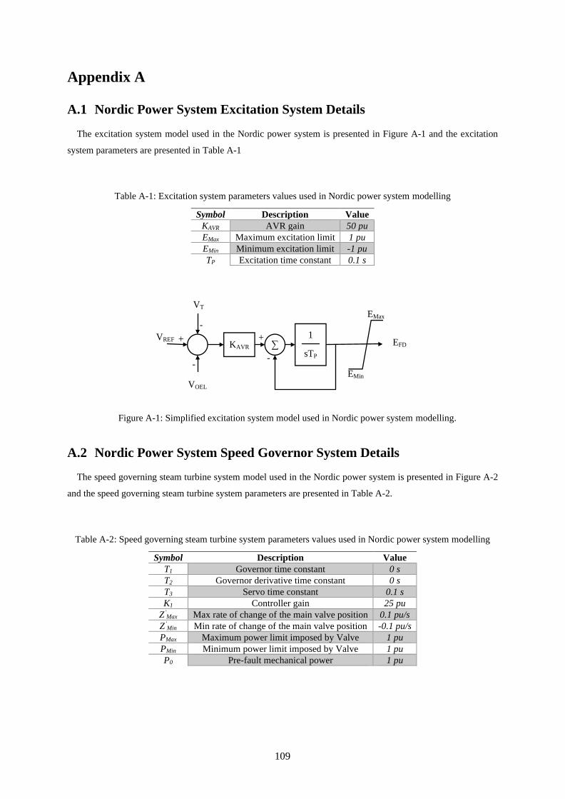
109

Appendix A

A.1 Nordic Power System Excitation System Details

The excitation system model used in the Nordic power system is presented in Figure A-1 and the excitation

system parameters are presented in Table A-1

Table A-1: Excitation system parameters values used in Nordic power system modelling

Symbol Description Value

KAVR AVR gain 50 pu

EMax Maximum excitation limit 1 pu

EMin Minimum excitation limit -1 pu

TP Excitation time constant 0.1 s

VREF

VT

VOEL

KAVR ∑

EMax

EMin

EFD+

-

+

-

-1

sTP

Figure A-1: Simplified excitation system model used in Nordic power system modelling.

A.2 Nordic Power System Speed Governor System Details

The speed governing steam turbine system model used in the Nordic power system is presented in Figure A-2

and the speed governing steam turbine system parameters are presented in Table A-2.

Table A-2: Speed governing steam turbine system parameters values used in Nordic power system modelling


T1 Governor time constant 0 s

T2 Governor derivative time constant 0 s

T3 Servo time constant 0.1 s

K1 Controller gain 25 pu

Z’Max Max rate of change of the main valve position 0.1 pu/s

Z’Min Min rate of change of the main valve position -0.1 pu/s

PMax Maximum power limit imposed by Valve 1 pu

PMin Minimum power limit imposed by Valve 1 pu

P0 Pre-fault mechanical power 1 pu

110

ωREF

P0

∑

Z’Max

Z’Min

PGV+

-

+

-

1

T3

ω

1 + sT1

K (1 + sT2) 1

s

PMax

PMin

-

Figure A-2: Simplified speed governing steam turbine system used in Nordic power system modelling.

A.3 Nordic Power System Steam Turbine System Details

The steam turbine system model used in the Nordic power system is presented in Figure A-3 and the steam

turbine system parameters are presented in Table A-3

Table A-3: Steam turbine system parameters values used in Nordic power system modelling


FHP High-pressure power fraction 0.4 pu

FIP Intermediate pressure power fraction 0.3 pu

FLP Low-pressure power fraction 0.3 pu

TCH Steam chest time constant 0.2 s

TRH Reheat time constant 4 s

TCO Crossover time constant 0.3 s

PGV Power at Gate or Valve outlet 1 pu

PM Mechanical Power 1 pu

FHP

∑

PGV

+

1 + sTCH

1

1 + sTRH

1

1 + sTCO

1

FHP FHP

∑PM

+ +

+

Figure A-3: Steam turbine system used in Nordic power system modelling.

A.4 Nordic Power System Overexcitation System Details

The value of Ecap, the thermal capability of each generator in the Nordic power system is presented in Table

A-4.

Table A-4: Thermal capability of the generator OEL system

Gen R (pu) Ifd Rated (pu) Ecap (pu) Gen R (pu) Ifd

Rated (pu) Ecap (pu)

g1 0.36 1.8087 48.365 g11 0.13 1.8087 48.365

g2 0.27 1.8087 48.365 g12 0.15 1.8087 48.365

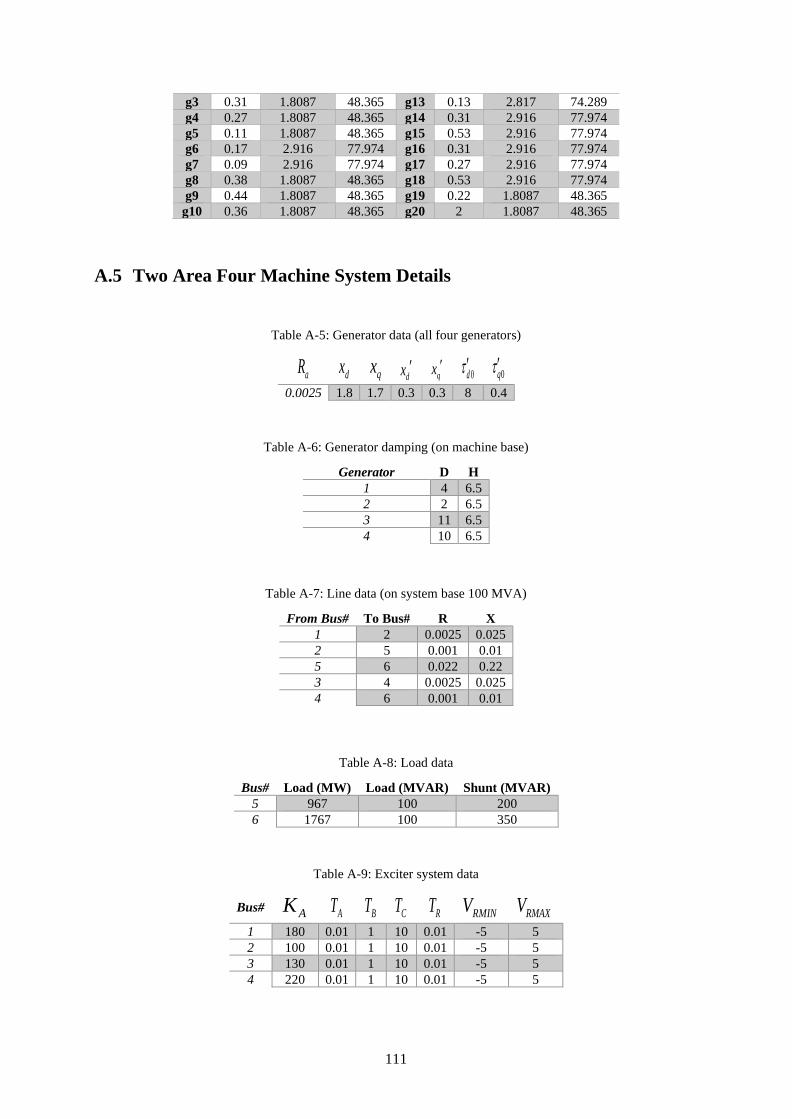
111

g3 0.31 1.8087 48.365 g13 0.13 2.817 74.289

g4 0.27 1.8087 48.365 g14 0.31 2.916 77.974

g5 0.11 1.8087 48.365 g15 0.53 2.916 77.974

g6 0.17 2.916 77.974 g16 0.31 2.916 77.974

g7 0.09 2.916 77.974 g17 0.27 2.916 77.974

g8 0.38 1.8087 48.365 g18 0.53 2.916 77.974

g9 0.44 1.8087 48.365 g19 0.22 1.8087 48.365

g10 0.36 1.8087 48.365 g20 2 1.8087 48.365

A.5 Two Area Four Machine System Details

Table A-5: Generator data (all four generators)

aR dx qx dx qx 0d 0q

0.0025 1.8 1.7 0.3 0.3 8 0.4

Table A-6: Generator damping (on machine base)

Generator D H

1 4 6.5

2 2 6.5

3 11 6.5

4 10 6.5

Table A-7: Line data (on system base 100 MVA)

From Bus# To Bus# R X

1 2 0.0025 0.025

2 5 0.001 0.01

5 6 0.022 0.22

3 4 0.0025 0.025

4 6 0.001 0.01

Table A-8: Load data

Bus# Load (MW) Load (MVAR) Shunt (MVAR)

5 967 100 200

6 1767 100 350

Table A-9: Exciter system data

Bus# AK AT BT CT RT RMINV RMAXV

1 180 0.01 1 10 0.01 -5 5

2 100 0.01 1 10 0.01 -5 5

3 130 0.01 1 10 0.01 -5 5

4 220 0.01 1 10 0.01 -5 5

emergency control for catastrophic disturbance in future

Documents