embedded optimization algorithms for perceptual enhancement of audio … · 2013-12-12 · in...
TRANSCRIPT

KU LEUVEN
FACULTEIT INGENIEURSWETENSCHAPPEN
DEPARTEMENT ELEKTROTECHNIEK
STADIUS CENTER FOR DYNAMICAL SYSTEMS,
SIGNAL PROCESSING AND DATA ANALYTICS
Kasteelpark Arenberg 10 – B-3001 Leuven
EMBEDDED OPTIMIZATION ALGORITHMS FOR
PERCEPTUAL ENHANCEMENT OF
AUDIO SIGNALS
Jury:
Prof. dr. C. Vandecasteele, voorzitter
Prof. dr. ir. P. Sas, vervangend voorzitter
Prof. dr. ir. M. Moonen, promotor
Prof. dr. M. Diehl, promotor
Prof. dr. ir. T. van Waterschoot, co-promotor
Prof. dr. ir. J. Suykens
Prof. dr. ir. P. Wambacq
Prof. dr. Y. Nesterov
(Universite catholique de Louvain, Belgium)
Prof. dr. ir. W. Verhelst
(Vrije Universiteit Brussel, Belgium)
Proefschrift voorgedragen
tot het behalen van de
graad van Doctor in de
Ingenieurswetenschappen
door
Bruno DEFRAENE
December 2013

c©2013 KU LEUVEN, Groep Wetenschap & TechnologieArenberg Doctoraatsschool, W. De Croylaan 6, B-3001 Heverlee, Belgie
Alle rechten voorbehouden. Niets uit deze uitgave mag vermenigvuldigd en/ofopenbaar gemaakt worden door middel van druk, fotocopie, microfilm, elektro-nisch of op welke andere wijze ook zonder voorafgaande schriftelijke toestem-ming van de uitgever.
All rights reserved. No part of the publication may be reproduced in any formby print, photoprint, microfilm or any other means without written permissionfrom the publisher.
ISBN 978-94-6018-779-7
D/2013/7515/160

Voorwoord
Achteromkijkend hangt een levensloop aaneen van de toevalligheden. Alseerstejaars masterstudent elektrotechniek was het dan ook eerder toevallig datik medio april 2008 tijdens de ESAT-eindwerkbeurs in gesprek raakte met Toonvan Waterschoot, die er de eindwerkvoorstellen van de DSP-groep aanprees.Een clipper ontwerpen voor audiosignalen? Klonk me heel interessant in deoren. Optimalisatie als voorgestelde aanpak voor het probleem? Vernieuwendidee! En dit alles onder een promotorenduo bestaande uit Prof. Marc Moonenen Prof. Moritz Diehl? Mijn eerste masterproefkeuze was beslist, hier wilde ikheel graag een academiejaar lang onderzoek naar doen. Die dag begon voor mij- zonder het zelf te beseffen - een wetenschappelijk en menselijk avontuur vol on-vergetelijke momenten, inspirerende ontmoetingen, en verhelderende inzichten,een verrassende rondreis die me onder andere naar het Verre Oosten en deMaghreb zou brengen.
Het succesvol vervullen van mijn doctoraatsonderzoek heeft - veel meer danmet toeval - vooral te maken met de uitstekende begeleiders, het boeiendeonderzoeksonderwerp, de fijne collega’s, en natuurlijk de onmisbare en onvoor-waardelijke steun van het thuisfront, die er samen hebben voor gezorgd dat vierjaar hard werken konden culmineren in deze doctoraatstekst. In wat volgt zouik graag alle mensen die me hierbij hebben geholpen oprecht willen bedanken.
Vooreerst zou ik mijn promotoren willen bedanken voor hun uitstekende begelei-ding van mijn onderzoek. Prof. Marc Moonen wil ik bedanken om me de kanste geven om onder zijn promotorschap een doctoraat te maken in zijn - hetmag gezegd - gerenommeerde onderzoeksgroep. Zijn uitstekende lessen overdigitale (audio)-signaalverwerking hebben me reeds tijdens mijn ingenieurso-pleiding geboeid en gevormd. Marc, heel erg bedankt om doorheen het docto-raat in mij te geloven, voor de talloze ideeen die tijdens onze vrijdagse meetingszijn ontstaan, voor je visie om op het gepaste moment de onderzoeksrichtingbij te sturen, voor je uitstekende correcties die mijn teksten stuk voor stukpublicatierijp hebben gemaakt, en voor de zin voor detail, structuur en kritiekdie je me hebt bijgebracht.
i
ii Voorwoord
Prof. Moritz Diehl zou ik willen bedanken om me als promotor met een onge-evenaard enthousiasme de weg te wijzen in het domein van de wiskundige op-timalisatie. De vele onderzoeksideeen die hij gelanceerd heeft, de contacten diehij voor mij gelegd heeft met vooraanstaande optimalisatiespecialisten binnenen buiten OPTEC, en de steeds opbouwende kritische blik waarmee de eersteversie van publicaties werden doorgelicht, hebben in hoge mate bijgedragen aande behaalde onderzoeksresultaten. Van harte bedankt hiervoor, Moritz.
Prof. Toon van Waterschoot wil ik graag bedanken voor de uitzonderlijk goedemanier waarop hij zowel mijn masterproef en doctoraatsonderzoek heeft bege-leid. Toon heeft me ingewijd in het verrichten van wetenschappelijk onderzoek,in het duidelijk synthetiseren en rapporteren, in het begeleiden van master-proefstudenten, en in ontelbare andere dingen waarin hij voor mij gedurendevijf jaar een inspirerende leermeester is geweest. Toon, ik heb enorm veelopgestoken van onze nauwe samenwerking, bedankt voor alles!
Ik zou ook de leden van de examencommissie hartelijk willen danken voor hunbereidheid om deel uit te maken van de jury, voor de kritische lezing van mijnproefschrift, en voor de interessante suggesties voor verbetering. Dear Prof. Jo-han Suykens, Prof. Patrick Wambacq, Prof. Werner Verhelst. Prof. Yurii Nes-terov, Prof. Carlo Vandecasteele, Prof. Paul Sas, I want to thank all of youfor being part of my examination committee and for providing your valuablesuggestions for the improvement of this manuscript.
Ik heb tijdens mijn doctoraat de eer gehad om samen te mogen werken metverschillende onderzoekers die elk met hun eigen expertise een belangrijke con-tributie hebben geleverd aan de behaalde onderzoeksresultaten. Dr. HansJoachim Ferreau, thank you for introducing me to the art of QP solving inthe early stages of my PhD. Dr. Andrea Suardi, thank you so much for yourtime and efforts spent at successfully implementing the clipping algorithm inhardware. Dr. Kim Ngo, thank you for our fruitful cooperation on the speechenhancement project. Naim Mansour en Steven De Hertogh wil ik bedankenvoor de vlotte samenwerking tijdens maar ook na het afleggen van hun uitmun-tende masterproef.
Graag zou ik ook de collega’s binnen de DSP-onderzoeksgroep willen bedanken,die samen gezorgd hebben voor een heel leuke en kameraadschappelijke sfeer,waarin het altijd prettig werken was. De fijne herinneringen aan mijn vierjaren in deze unieke groep zijn legio (en beperken zich niet tot binnen demuren van het departement): ik denk onwillekeurig aan het jaarlijkse ESAT-voetbaltornooi waarin deelnemen achteraf toch een pak belangrijker bleek danwinnen, aan de conferenties in dichtbije of avontuurlijk verre buitenlanden,aan de leuke etentjes, en natuurlijk aan de legendarische housewarmings enfeestjes in het decor van de Leuvense binnenstad. Paschalis, bedankt om alsvaste bureaugenoot altijd klaar te staan met goede raad, voor onze interes-sante gesprekken, voor het voortdurend delen van je inzichten en ervaring.

iii
Alexander en Bram, bedankt om een lichtend voorbeeld te vormen van hoe jeeen doctoraat tot een (zeer) succesvol einde brengt, en natuurlijk ook voor degezamenlijke Alma-bezoeken die steeds een zeer aangenaam rustpunt in de dagvormden.
Rodrigo, Joe, Javier, Pepe, Amir, thanks for all the nice moments we haveshared within and outside of ESAT. Beier and Lulu, it was truly an honourfor me to attend your wedding party in Beijing, the visit to China with Bramand Pieter was an unforgettable experience, for which I thank you with all ofmy heart. I would like to thank all my colleagues for creating such a nice workatmosphere throughout the years: thank you Aldona, Amin, Ann, Deepak, Enzo,Gert, Giacomo, Giuliano, Hanne, Johnny, Jorge, Kristian, Marijn, Nejem,Niccolo, Prabin, Rodolfo, Romain, Sylwek, Wouter, and Yi!
Ik zou ook een woord van dank willen richten aan de collega’s die het departe-ment ESAT en de afdeling STADIUS (formerly known as SISTA) al die jarenlogistiek, organisatorisch en financieel vlot draaiende hebben gehouden: be-dankt Ida, Lut, Eliane, Evelyn, en Ilse voor jullie harde werk. John zou ikdaarnaast ook willen bedanken voor de vele momenten van gedeelde vreugde(vaak) en smart (heel soms) na de voetbalprestaties van ons geliefde RSC An-derlecht.
Mattia, I want to thank you for being an ever-enjoyable flatmate, I have trulyappreciated our years of shared ups and downs in the quest for a successfulPhD, as much as the memorable parties that were hosted in our apartment.
Ten slotte zou ik de mensen willen bedanken die me het dierbaarst zijn. Mama,papa, ik wil jullie hier oneindig bedanken voor de manier waarop jullie mijopgevoed hebben, voor jullie onvoorwaardelijke steun, geloof en interesse inalles wat ik doe, en voor alle goede raadgevingen die jullie me steeds weerhebben gegeven. Dit doctoraatsproefschrift tot een goed einde brengen zouzonder jullie onmogelijk zijn geweest. Papa, maman, je tiens a vous remercierinfiniment pour la facon dont vous m’ avez eleve, et pour votre soutien incon-ditionnel dans tout ce que je fais. Il aurait ete impossible de finir mon doctoratsans votre soutien. Gilles, jou wil ik bedanken om als grote broer voor mijhet pad te effenen en het goede voorbeeld te tonen als burgerlijk ingenieur,muzikant, en op vele andere vlakken, met het afwerken van dit proefschrift benik jou - voor de verandering - eens voorgegaan. Oma, bedankt voor de grotebetrokkenheid die je samen met Parrain altijd getoond hebt in alle stappen dieik heb gezet, voor het goede voorbeeld dat jullie me steeds getoond hebben, ende wijze raad en ervaring die jullie mij hebben doorgegeven. Marraine, mercibeaucoup pour ta generosite, ton accueil toujours aussi chaleureux, et pour toutce que tu m’as appris. Mijn oprechte dank gaat ook uit naar Anne, Philippe,Lotte, Jasper, Paulien, Gaby, Agnes, en alle andere familieleden die me altijdgesteund hebben.

iv Voorwoord
Lieve Sophie, jou wil ik danken voor je warme steun en liefde waarop ik inde laatste twee jaren altijd kon rekenen en die enorm veel voor mij betekenen,voor je onvoorwaardelijke geloof in mij, en voor alle prachtige momenten diewe samen al hebben gedeeld.
Het naderende einde van dit voorwoord betekent voor sommigen misschien hetsein om dit boek als gelezen te beschouwen. Diegenen die de voorgaande pa-gina’s echter doorworsteld hebben om eindelijk aan het interessantere leeswerkte beginnen, wens ik naast proficiat ook veel leesplezier, in de hoop dat deverderop beschreven ideeen en onderzoeksresultaten een bouwsteen kunnen vor-men voor nieuwe wetenschappelijke bevindingen.
Bruno Defraene
Leuven, December 2013

Abstract
This thesis investigates the design and evaluation of an embedded optimizationframework for the perceptual enhancement of audio signals which are degradedby linear and/or nonlinear distortion. In general, audio signal enhancementhas the goal to improve the perceived audio quality, speech intelligibility, oranother desired perceptual attribute of the distorted audio signal by applyinga real-time digital signal processing algorithm. In the designed embedded op-timization framework, the audio signal enhancement problem under consider-ation is formulated and solved as a per-frame numerical optimization problem,allowing to compute the enhanced audio signal frame that is optimal accordingto a desired perceptual attribute. The first stage of the embedded optimizationframework consists in the formulation of the per-frame optimization problemaimed at maximally enhancing the desired perceptual attribute, by explicitlyincorporating a suitable model of human sound perception. The second stageof the embedded optimization framework consists in the on-line solution ofthe formulated per-frame optimization problem, by using a fast and reliableoptimization method that exploits the inherent structure of the optimizationproblem. This embedded optimization framework is applied to four commonlyencountered and challenging audio signal enhancement problems, namely hardclipping precompensation, loudspeaker precompensation, declipping and multi-microphone dereverberation.
The first part of this thesis focuses on precompensation algorithms, in whichthe audio signal enhancement operation is applied before the distortion pro-cess affects the audio signal. More specifically, the problems of hard clippingprecompensation and loudspeaker precompensation are tackled in the embed-ded optimization framework. In the context of hard clipping precompensation,an objective function reflecting the perceptible nonlinear hard clipping distor-tion is constructed by including frequency weights based on the instantaneousmasking threshold, which is computed on a frame-by frame basis by applyinga perceptual model. The resulting per-frame convex quadratic optimizationproblems are solved efficiently using an optimal projected gradient method,for which theoretical complexity bounds are derived. Moreover, a fixed-pointhardware implementation of this optimal projected gradient method on a field
v
vi Abstract
programmable gate array (FPGA) shows the algorithm to be capable to run inreal time and without perceptible audio quality loss on a small and portableaudio device. In the context of loudspeaker precompensation, an objectivefunction reflecting the perceptible combined linear and nonlinear loudspeakerdistortion is constructed in a similar fashion as for hard clipping precompensa-tion. The loudspeaker is modeled using a Hammerstein loudspeaker model, i.e.a cascade of a memoryless nonlinearity and a linear FIR filter. The resultingper-frame nonconvex optimization problems are solved efficiently using gradi-ent optimization methods which exploit knowledge on the invertibility and thesmoothness of the memoryless nonlinearity in the Hammerstein loudspeakermodel. From objective and subjective evaluation experiments, it is concludedwith statistical significance that the embedded optimization algorithms for hardclipping and loudspeaker precompensation improve the resulting audio qualitywhen compared to standard precompensation algorithms.
The second part of this thesis focuses on recovery algorithms, in which theaudio signal enhancement operation is applied after the distortion process af-fects the audio signal. More specifically, the problems of declipping and multi-microphone dereverberation are tackled in the embedded optimization frame-work. Declipping is formulated as a sparse signal recovery problem where therecovery is performed by solving a per-frame ℓ1-norm minimization problem,which includes frequency weights based on the instantaneous masking thresh-old. As a result, the declipping algorithm is focused on maximizing the per-ceived audio quality instead of the physical signal reconstruction quality ofthe declipped audio signal. Comparative objective and subjective evaluationexperiments reveal with statistical significance that the proposed embeddedoptimization declipping algorithm improves the resulting audio quality com-pared to existing declipping algorithms. Multi-microphone dereverberation isformulated as a nonconvex optimization problem, allowing for the joint estima-tion of the clean audio signal and the room acoustics model parameters. It isshown that the nonconvex optimization problem can be smoothed by includ-ing regularization terms based on a statistical late reverberation model and asparsity prior for the clean audio signal, which is demonstrated to improve thedereverberation performance.

Korte Inhoud
Dit doctoraatsproefschrift onderzoekt het ontwerp en de evaluatie van een in-gebedde optimalisatieraamwerk voor de perceptuele verbetering van geluidssig-nalen die aangetast zijn door lineaire en niet-lineaire distortie. In het alge-meen heeft signaalverbetering als doel om de geluidskwaliteit, spraakverstaan-baarheid, of een andere gewenste perceptuele eigenschap van het geluidssignaalte verbeteren door het toepassen van een digitaal signaalverwerkingsalgoritmein reele tijd. In het ontworpen ingebedde optimalisatieraamwerk wordt hetbeschouwde signaalverbeteringsprobleem geformuleerd en opgelost als een nu-meriek optimalisatieprobleem per signaalvenster, wat toelaat om het verbeterdesignaalvenster te berekenen dat optimaal is volgens een gewenste perceptueleeigenschap. De eerste fase van het ingebedde optimalisatieraamwerk bestaatin de formulering van het optimalisatieprobleem per signaalvenster, en is eropgericht om de gewenste perceptuele eigenschap maximaal te verbeteren, doorhet toepassen van een geschikt model van de menselijke perceptie van geluid.De tweede fase van het ingebedde optimalisatieraamwerk bestaat in de on-line oplossing van het geformuleerde optimalisatieprobleem per signaalvenster,door het aanwenden van een snelle en betrouwbare optimalisatiemethode diede inherente structuur van het optimalisatieprobleem uitbuit. Dit ingebeddeoptimalisatieraamwerk wordt toegepast op vier courante en uitdagende sig-naalverbeteringsproblemen, namelijk de precompensatie van hard clipping, deprecompensatie van luidsprekers, declipping, en meer-microfoons dereverbera-tie.
Het eerste deel van dit doctoraatsproefschrift spitst zich toe op algoritmes voorsignaalprecompensatie, waarbij het geluidssignaal wordt verbeterd voordat dedistortie inwerkt op het geluidssignaal. Meer specifiek worden de precom-pensatie van hard clipping en de precompensatie van luidsprekers als afzon-derlijke problemen binnen het ingebedde optimalisatieraamwerk beschouwd.In het kader van de precompensatie van hard clipping, wordt een doelfunc-tie opgesteld die de waarneembare niet-lineaire hard clipping distortie weer-spiegelt, door het toepassen van frequentiegewichten gebaseerd op de instan-tane maskeringsdrempel. Deze maskeringsdrempel wordt per signaalvensterberekend via een perceptueel model. Het resulterende convexe kwadratische
vii

viii Korte Inhoud
optimalisatieprobleem per signaalvenster wordt doeltreffend opgelost via eenoptimale geprojecteerde gradientmethode, waarvoor theoretische complexiteits-grenzen worden opgesteld. Daarenboven toont een hardware implementatie invaste komma van de optimale geprojecteerde gradientmethode op een field pro-grammable gate array (FPGA) aan dat het algoritme in reele tijd en zonderwaarneembaar geluidskwaliteitsverlies kan uitgevoerd worden op een klein endraagbaar audiotoestel. In het kader van de precompensatie van luidsprekers,wordt een doelfunctie opgesteld die de gecombineerde waarneembare lineaire enniet-lineaire luidsprekerdistortie weerspiegelt, op een gelijkaardige manier alsvoor de precompensatie van hard clipping. De luidspreker wordt gemodelleerddoor een Hammerstein luidsprekermodel, dat bestaat uit de opeenvolging vaneen geheugenloze niet-lineariteit en een lineair FIR filter. Het resulterende niet-convexe optimalisatieprobleem per signaalvenster wordt doeltreffend opgelostvia gradientmethodes die kennis uitbuiten over de inverteerbaarheid en glad-heid van de geheugenloze niet-lineariteit in het Hammerstein luidsprekermodel.Objectieve en subjectieve evaluatie-experimenten laten toe om met statistischesignificantie te besluiten dat de ingebedde optimalisatiealgoritmes voor de pre-compensatie van hard clipping en luidsprekers de geluidskwaliteit verbeterenten opzichte van bestaande algoritmes voor precompensatie.
Het tweede deel van dit doctoraatsproefschrift spitst zich toe op algoritmesvoor signaalherstel, waarbij het geluidssignaal wordt verbeterd nadat de dis-tortie heeft ingewerkt op het geluidssignaal. Meer bepaald worden declippingen meermicrofoons dereverberatie als afzonderlijke problemen binnen het in-gebedde optimalisatieraamwerk beschouwd. Declipping wordt geformuleerd alseen ijl signaalherstelprobleem, waarin het signaalherstel uitgevoerd wordt doorhet oplossen van een ℓ1-norm minimalisatieprobleem per signaalvenster. Ditminimalisatieprobleem bevat frequentiegewichten gebaseerd op de instantanemaskeringsdrempel. Zodoende poogt het declipping algoritme de geluidskwa-liteit maximaal te verbeteren, in plaats van te focussen op de fysieke recon-structiekwaliteit van het geluidssignaal. Vergelijkende objectieve en subjectieveevaluatie-experimenten laten toe om met statistische significantie te besluitendat het ingebedde optimalisatiealgoritme voor declipping de geluidskwaliteitverbetert ten opzichte van bestaande algoritmes. Meermicrofoons dereverbera-tie wordt geformuleerd als een niet-convex optimalisatieprobleem dat toelaatom gelijktijdig het zuivere geluidssignaal en de parameters van de kamerakoes-tiek te schatten. Het niet-convexe optimalisatieprobleem kan verzacht wordendoor regularisatietermen toe te voegen die gebaseerd zijn op een statistischmodel voor late reverberatie en een ijlheidsveronderstelling van het zuiveregeluidssignaal, die samen de performantie van dereverberatie aantoonbaar ver-hogen.
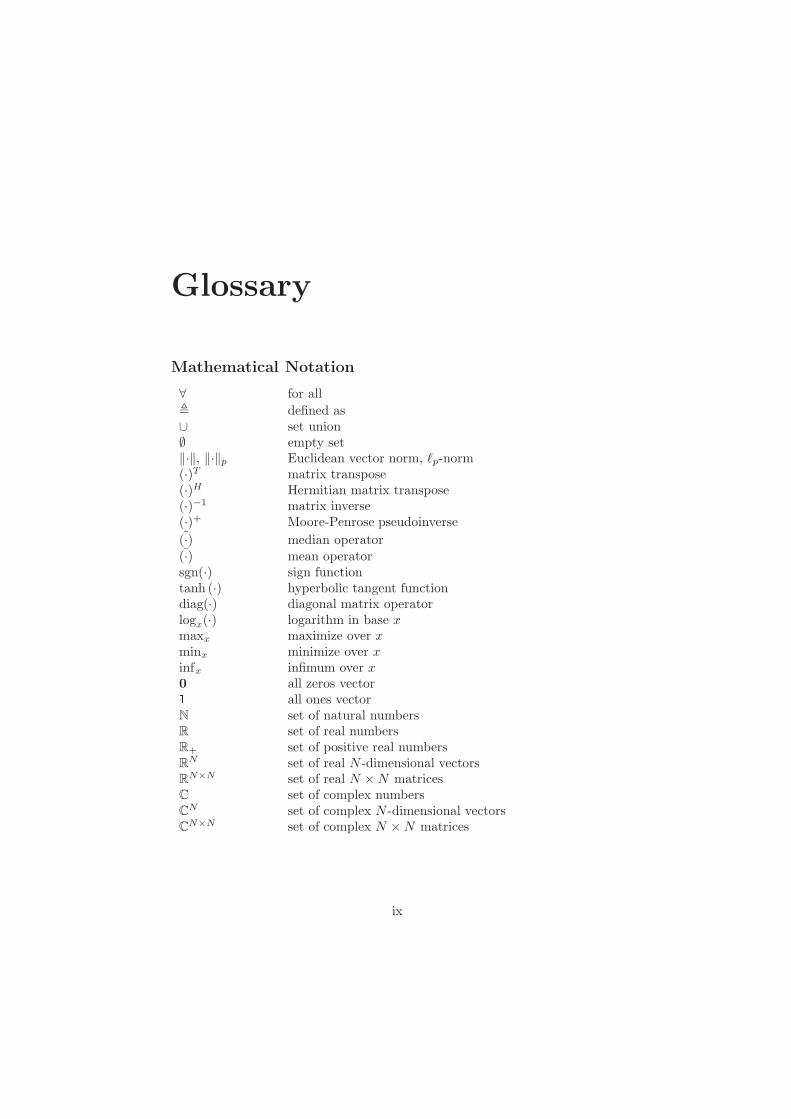
Glossary
Mathematical Notation
∀ for all
, defined as∪ set union∅ empty set‖·‖, ‖·‖p Euclidean vector norm, ℓp-norm(·)T matrix transpose(·)H Hermitian matrix transpose(·)−1 matrix inverse(·)+ Moore-Penrose pseudoinverse
(·) median operator(·) mean operatorsgn(·) sign functiontanh (·) hyperbolic tangent functiondiag(·) diagonal matrix operatorlogx(·) logarithm in base xmaxx maximize over xminx minimize over xinfx infimum over x0 all zeros vector1 all ones vectorN set of natural numbersR set of real numbersR+ set of positive real numbersR
N set of real N -dimensional vectorsRN×N set of real N ×N matricesC set of complex numbersCN set of complex N -dimensional vectorsCN×N set of complex N ×N matrices
ix

x Glossary
∇(·) gradient operator∇2(·) Hessian operator⊗ Kronecker product
Fixed Symbols
ai sensing matrix columnA sensing matrixAm loudspeaker precompensation Hessian matrixb number of fraction bitsbi fraction bitbm loudspeaker precompensation gradient vectorciter latency per iteration in clock cyclesctotal overall latency in clock cyclesckm auxiliary audio signal frame iterateCm Lipschitz constantC+
m row selection matrix corresponding to positively clippedsamples
C−m row selection matrix corresponding to negatively clipped
samplesdm distance measured∗ optimal dual objective valueD function domainD unitary DFT matrixe Euler’s numberei decimal exponent bite error signal vectorE decimal exponentE[·] expected value operatorf(·) objective functionf(·) distortion processg(·) per-sample memoryless nonlinearityg(·) per-frame memoryless nonlinearityg−1(·) inverse per-sample memoryless nonlinearityg−1(·) inverse per-frame memoryless nonlinearityh[n] finite impulse responseh RIR vectorH0 statistical null hypothesisH1 statistical alternative hypothesis (Ch. 2)Ha statistical alternative hypothesis (Ch. 4,6)H0 RIR matrix
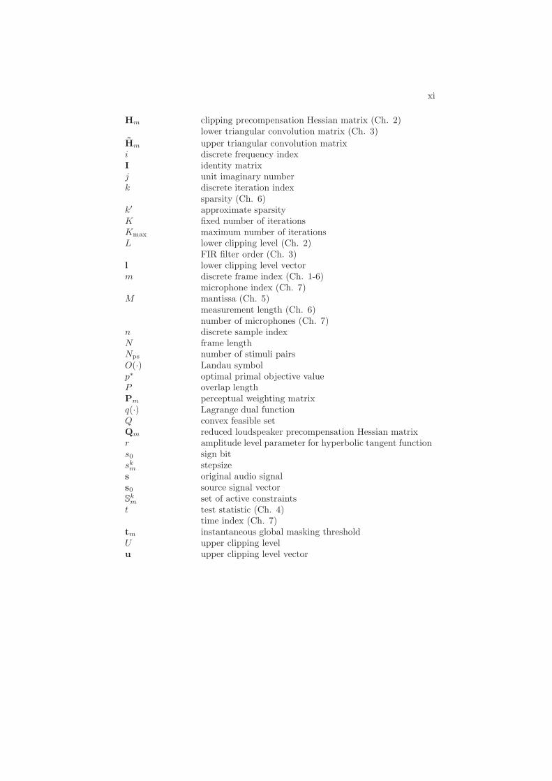
xi
Hm clipping precompensation Hessian matrix (Ch. 2)lower triangular convolution matrix (Ch. 3)
Hm upper triangular convolution matrixi discrete frequency indexI identity matrixj unit imaginary numberk discrete iteration index
sparsity (Ch. 6)k′ approximate sparsityK fixed number of iterationsKmax maximum number of iterationsL lower clipping level (Ch. 2)
FIR filter order (Ch. 3)l lower clipping level vectorm discrete frame index (Ch. 1-6)
microphone index (Ch. 7)M mantissa (Ch. 5)
measurement length (Ch. 6)number of microphones (Ch. 7)
n discrete sample indexN frame lengthNps number of stimuli pairsO(·) Landau symbolp∗ optimal primal objective valueP overlap lengthPm perceptual weighting matrixq(·) Lagrange dual functionQ convex feasible setQm reduced loudspeaker precompensation Hessian matrixr amplitude level parameter for hyperbolic tangent functions0 sign bitskm stepsizes original audio signals0 source signal vectorSkm set of active constraintst test statistic (Ch. 4)
time index (Ch. 7)tm instantaneous global masking thresholdU upper clipping levelu upper clipping level vector
xii Glossary
v precompensated audio signalvm precompensated audio signal frameVfix fixed point valueVfloat floating point valueV
km set of violated constraints
wm perceptual weighting functionWm perceptual weighting matrixx[n] discrete time-domain clean audio signalXm(ejωi) discrete frequency-domain clean audio signalx clean audio signalxm clean audio signal framey[n] discrete time-domain distorted audio signalYm(ejωi) discrete frequency-domain distorted audio signaly distorted audio signalym distorted audio signal frameykm distorted audio signal frame iteratey∗[n] discrete time-domain enhanced audio signaly∗ enhanced audio signaly∗m enhanced audio signal frameα compression parameterαJB significance level for Jarque-Bera statistical normality testαTT significance level for statistical t-testβ relaxation of the gradient for Armijo conditionβi(·) eigenvalue operatorγm regularization parameterγkm optimal projected gradient method auxiliary weightδkm optimal projected gradient method weightδ optimal projected gradient method weight vectorǫ solution accuracyǫm relaxation parameterη fixed number of iterations (Ch. 2)
backtracking factor for Armijo line search (Ch. 3)θc clipping levelθ distortion model parameters
θ estimated distortion model parametersκm condition numberλi(·) eigenvalue operatorλ Lagrange multiplier associated to inequality constraintλ Lagrange multiplier vector associated to inequality con-
straints

xiii
λm,l Lagrange multiplier vector associated to lower clippinglevel constraints
λm,u Lagrange multiplier vector associated to upper clippinglevel constraints
µ(·) coherence measureµm convexity parameterν Lagrange multiplier associated to equality constraintν Lagrange multiplier vector associated to equality con-
straintsπ Archimedes’ constantΠQ(·) orthogonal projection onto set Qρ population Pearson correlation coefficientρ sample Pearson correlation coefficientσi(·) singular value operator∑N
n=1 summation operatorΦ measurement matrixΨ fixed basisωi discrete frequency variableΩ convex feasible setL(·) Lagrangian function
Acronyms and Abbreviations
ADC analog-to-digital converterBCD block coordinate descentBP Basis PursuitCCR Comparison Category RatingCD compact discCF clipping factorCLB Configurable Logic BlockCS Compressed SensingCSL0 CS-based declipping using ℓ0-norm optimizationCSL1 CS-based declipping using ℓ1-norm optimizationDAC digital-to-analog converterdB decibelDCR Degradation Category RatingDCT Discrete Cosine TransformDFT Discrete Fourier TransformDSP digital signal processinge.g. exempli gratia: for exampleFF flip-flopFFT Fast Fourier Transform

xiv Glossary
FIR Finite Impulse ResponseFPGA field programmable gate arrayHLS high-level synthesisHz hertzi.e. id est : that isIFFT Inverse Fast Fourier TransformIIR Infinite Impulse ResponseIP Intellectual PropertykHz kilohertzℓ1/ℓ2-RNLS NLS with ℓ1-norm and ℓ2-norm regularizationℓ2-RNLS NLS with ℓ2-norm regularizationLAB Logic Array BlockLUT lookup tableMDCR Mean Degradation Category RatingMHz megahertzms millisecondsMSE mean-squared errormW milliwattNLS nonlinear least squaresODG Objective Difference GradeOMP Orthogonal Matching PursuitPCS Perceptual Compressed SensingPCSL1 PCS-based declipping using ℓ1-norm optimizationPEAQ Perceptual Evaluation of Audio QualityPSD power spectral densityQP quadratic programRIP restricted isometry propertyRIR room impulse responseRTL register-transfer levels secondss.t. subject toSCP sequential cone programmingSNR signal-to-noise ratioSPL Sound Pressure LevelSQP sequential quadratic programmingVHDL VHSIC Hardware Description LanguageVHSIC very-high-speed integrated circuitsW WattXPE Xilinx Power Estimatorµs microseconds

xv

xvi Glossary

Contents
Voorwoord i
Abstract v
Korte Inhoud vii
Glossary ix
Contents xvii
I Introduction
1 Introduction 3
1.1 Problem Statement and Motivation . . . . . . . . . . . . . . . . 4
1.1.1 Audio Signal Distortion . . . . . . . . . . . . . . . . . . 4
1.1.2 Impact on Sound Perception . . . . . . . . . . . . . . . 7
1.1.3 Audio Signal Enhancement . . . . . . . . . . . . . . . . 9
1.2 Precompensation Algorithms . . . . . . . . . . . . . . . . . . . 11
1.2.1 Hard Clipping Precompensation . . . . . . . . . . . . . 11
1.2.2 Loudspeaker Precompensation . . . . . . . . . . . . . . 14
1.3 Recovery Algorithms . . . . . . . . . . . . . . . . . . . . . . . . 17
xvii

xviii Contents
1.3.1 Declipping . . . . . . . . . . . . . . . . . . . . . . . . . . 17
1.3.2 Dereverberation . . . . . . . . . . . . . . . . . . . . . . 19
1.4 Embedded Optimization Framework for Audio Signal Enhance-ment . . . . . . . . . . . . . . . . . . . . . . . . . . . . . . . . . 21
1.4.1 Embedded Optimization . . . . . . . . . . . . . . . . . . 22
1.4.2 Perceptual Models . . . . . . . . . . . . . . . . . . . . . 23
1.4.3 Main Research Objectives . . . . . . . . . . . . . . . . . 26
1.5 Thesis Outline and Publications . . . . . . . . . . . . . . . . . . 26
1.5.1 Chapter-By-Chapter Outline and Contributions . . . . . 26
1.5.2 Included Publications . . . . . . . . . . . . . . . . . . . 29
Bibliography . . . . . . . . . . . . . . . . . . . . . . . . . . . . . . . 30
II Precompensation Algorithms
2 Hard Clipping Precompensation 43
2.1 Introduction . . . . . . . . . . . . . . . . . . . . . . . . . . . . . 45
2.2 Perception-Based Clipping . . . . . . . . . . . . . . . . . . . . . 48
2.2.1 General Description of the Algorithm . . . . . . . . . . 48
2.2.2 Optimization Problem Formulation . . . . . . . . . . . . 49
2.2.3 Perceptual Weighting Function . . . . . . . . . . . . . . 50
2.3 Optimization Methods . . . . . . . . . . . . . . . . . . . . . . . 53
2.3.1 Convex Optimization Framework . . . . . . . . . . . . . 54
2.3.2 Dual Active Set Strategy . . . . . . . . . . . . . . . . . 56
2.3.3 Projected Gradient Descent . . . . . . . . . . . . . . . . 59
2.3.4 Optimal Projected Gradient Descent . . . . . . . . . . . 63
2.4 Simulation Results . . . . . . . . . . . . . . . . . . . . . . . . . 66
2.4.1 Comparative Evaluation of Perceived Audio Quality . . 66

Contents xix
2.4.2 Experimental Evaluation of Algorithmic Complexity . . 72
2.4.3 Applicability in Real-Time Context . . . . . . . . . . . . 73
2.5 Conclusions . . . . . . . . . . . . . . . . . . . . . . . . . . . . . 75
Bibliography . . . . . . . . . . . . . . . . . . . . . . . . . . . . . . . 76
3 Loudspeaker Precompensation 79
3.1 Introduction . . . . . . . . . . . . . . . . . . . . . . . . . . . . . 81
3.2 Embedded-Optimization-Based Precompensation . . . . . . . . 82
3.2.1 Hammerstein Model Description . . . . . . . . . . . . . 82
3.2.2 Embedded-Optimization-Based Precompensation . . . . 84
3.2.3 Perceptual Weighting Function . . . . . . . . . . . . . . 86
3.3 Optimization Methods . . . . . . . . . . . . . . . . . . . . . . . 88
3.3.1 Classes of Memoryless Nonlinearities . . . . . . . . . . . 88
3.3.2 Invertible Memoryless Nonlinearities . . . . . . . . . . . 89
3.3.3 Non-Invertible Smooth Memoryless Nonlinearities . . . 91
3.3.4 Non-Invertible Hard Clipping Memoryless Nonlinearities 92
3.3.5 Algorithmic Complexity Bounds . . . . . . . . . . . . . 96
3.4 Audio Quality Evaluation . . . . . . . . . . . . . . . . . . . . . 97
3.4.1 Synthetic Hammerstein Loudspeaker Models . . . . . . 97
3.4.2 Identified Hammerstein Loudspeaker Models . . . . . . 100
3.4.3 Identification of Hammerstein Model Parameters . . . . 104
3.5 Conclusions . . . . . . . . . . . . . . . . . . . . . . . . . . . . . 105
Bibliography . . . . . . . . . . . . . . . . . . . . . . . . . . . . . . . 105
4 Subjective Audio Quality Evaluation 109
4.1 Introduction . . . . . . . . . . . . . . . . . . . . . . . . . . . . . 109
4.2 Research Questions and Hypotheses . . . . . . . . . . . . . . . 110
xx Contents
4.3 Experimental Design and Set-up . . . . . . . . . . . . . . . . . 112
4.4 Results and Statistical Analysis . . . . . . . . . . . . . . . . . . 116
4.4.1 Test Subject Responses . . . . . . . . . . . . . . . . . . 116
4.4.2 Statistical Hypothesis Testing . . . . . . . . . . . . . . . 116
4.4.3 Correlation Between Subjective and Objective Scores . 118
4.5 Conclusions . . . . . . . . . . . . . . . . . . . . . . . . . . . . . 119
Bibliography . . . . . . . . . . . . . . . . . . . . . . . . . . . . . . . 121
5 Embedded Hardware Implementation 123
5.1 Introduction . . . . . . . . . . . . . . . . . . . . . . . . . . . . . 123
5.2 Embedded Hardware Architecture . . . . . . . . . . . . . . . . 124
5.2.1 Optimal Projected Gradient Algorithm . . . . . . . . . 124
5.2.2 FPGA Implementation Architecture . . . . . . . . . . . 125
5.3 FPGA Implementation Aspects . . . . . . . . . . . . . . . . . . 127
5.3.1 Floating-Point and Fixed-Point Arithmetic . . . . . . . 127
5.3.2 Fast Fourier Transform . . . . . . . . . . . . . . . . . . 130
5.4 Simulation Results . . . . . . . . . . . . . . . . . . . . . . . . . 132
5.4.1 Simulation Set-up . . . . . . . . . . . . . . . . . . . . . 132
5.4.2 Accuracy in Fixed-Point Arithmetic . . . . . . . . . . . 133
5.4.3 Latency, Resource Usage and Power Consumption . . . 134
5.5 Conclusions . . . . . . . . . . . . . . . . . . . . . . . . . . . . . 139
Bibliography . . . . . . . . . . . . . . . . . . . . . . . . . . . . . . . 139
III Recovery Algorithms
6 Declipping Using Perceptual Compressed Sensing 143
6.1 Introduction . . . . . . . . . . . . . . . . . . . . . . . . . . . . . 145

Contents xxi
6.2 A CS Framework for Declipping . . . . . . . . . . . . . . . . . . 146
6.2.1 CS Basic Principles . . . . . . . . . . . . . . . . . . . . 147
6.2.2 Perfect Recovery Guarantees . . . . . . . . . . . . . . . 148
6.2.3 CS-Based Declipping . . . . . . . . . . . . . . . . . . . . 149
6.3 A PCS Framework for Declipping . . . . . . . . . . . . . . . . . 152
6.3.1 Perceptual CS Framework . . . . . . . . . . . . . . . . . 152
6.3.2 Masking Threshold Calculation . . . . . . . . . . . . . . 154
6.3.3 PCS-Based Declipping Using ℓ1-norm Optimization . . 155
6.4 Evaluation . . . . . . . . . . . . . . . . . . . . . . . . . . . . . . 157
6.4.1 Objective Evaluation . . . . . . . . . . . . . . . . . . . . 157
6.4.2 Impact of Regularisation Parameter γm . . . . . . . . . 163
6.4.3 Impact of Masking Threshold Estimation Procedure . . 163
6.4.4 Subjective Evaluation . . . . . . . . . . . . . . . . . . . 164
6.4.5 Suitability of PEAQ ODG as Objective Measure . . . . 169
6.5 Conclusions . . . . . . . . . . . . . . . . . . . . . . . . . . . . . 169
Bibliography . . . . . . . . . . . . . . . . . . . . . . . . . . . . . . . 170
7 Multi-Microphone Dereverberation 175
7.1 Introduction . . . . . . . . . . . . . . . . . . . . . . . . . . . . . 177
7.2 Problem Statement . . . . . . . . . . . . . . . . . . . . . . . . . 178
7.3 Embedded Optimization Algorithms . . . . . . . . . . . . . . . 180
7.3.1 NLS problem . . . . . . . . . . . . . . . . . . . . . . . . 181
7.3.2 ℓ2-regularized NLS problem . . . . . . . . . . . . . . . . 181
7.3.3 ℓ1/ℓ2-regularized NLS problem . . . . . . . . . . . . . . 182
7.4 Evaluation . . . . . . . . . . . . . . . . . . . . . . . . . . . . . . 183
7.5 Conclusions . . . . . . . . . . . . . . . . . . . . . . . . . . . . . 184
Bibliography . . . . . . . . . . . . . . . . . . . . . . . . . . . . . . . 185

xxii Contents
8 Conclusions and Suggestions for Future Research 187
8.1 Summary and Conclusions . . . . . . . . . . . . . . . . . . . . . 187
8.2 Suggestions for Future Research . . . . . . . . . . . . . . . . . . 190
Bibliography . . . . . . . . . . . . . . . . . . . . . . . . . . . . . . . 192
Publication List 193
Curriculum Vitae 197

Part I
Introduction

2

Chapter 1
Introduction
When listening to music through a portable music player, a laptop, or a publicaddress system, sound quality and clarity are crucial factors to make it anenjoyable experience. When hearing the voice of the person you are speaking tothrough a mobile phone, a teleconferencing system, or a hearing aid, the qualityand intelligibility of the speech are decisive for a satisfactory and effectivecommunication. Before reaching the ear, music and speech signals have passedthrough many stages in the so-called audio signal path, e.g. from the recordingdevice over the transmission channel to a reproduction device. Throughout thisaudio signal path, there is an abundance of potential audio signal distortionmechanisms, which can have a negative effect on the quality and intelligibilityof the perceived audio signal. This makes it indispensable to design and applyeffective audio signal enhancement algorithms for improving the quality orintelligibility of audio signals that are degraded by a given distortion process,by applying some form of real-time digital signal processing.
This introduction is organized as follows. In Section 1.1, the major distortionmechanisms along a typical audio signal path will be pointed out and theirimpact on sound perception will be discussed. In Sections 1.2 and 1.3, the stateof the art and the prevailing challenges for audio signal enhancement algorithmswill be reviewed. In Section 1.4, a novel audio signal enhancement frameworkfor overcoming the limitations of existing audio signal enhancement algorithmsis outlined, which is based on the application of embedded optimization andperceptual models. The design of this embedded optimization framework andits application to different audio signal enhancement problems form the topicof this thesis.
3

4 Introduction
Figure 1.1: Stages in the audio signal path.
1.1 Problem Statement and Motivation
1.1.1 Audio Signal Distortion
Audio signal distortion can be defined as any alteration occurring in the time-domain waveform or frequency spectrum of an audio signal. Although in certaincases the distortion is applied intentionally to create a desired audio effect suchas a distorted guitar sound, vocal reverberation, or a change of the audio signaltimbre [1], in general the occurence of audio signal distortion is unintentionaland undesired. Audio signal distortion can be broadly classified into two types,namely linear distortion and nonlinear distortion. Linear distortion involveschanges in the relative amplitudes and phases of the frequency componentsconstituting the original audio signal. Nonlinear distortion involves the intro-duction of frequency components that were not present in the original audiosignal [2].
Linear and nonlinear distortion can be introduced at different stages along theaudio signal path transforming the clean audio signal into the reproduced audiosignal, as shown in Figure 1.11.
Room acoustics
In a first stage, the room acoustics form a potential source of audio signaldistortion. When the clean audio signal is produced in a closed acoustic envi-ronment, it is partially reflected by the phyisical boundaries of the environment,i.e. by the walls, the floor, and ceiling of the room. As a result, not only theclean audio signal is picked up by the recording device, but also several de-layed and attenuated replicas of the clean audio signal. This effect is known asreverberation and is a form of linear distortion [3].
1Note that not all stages in the audio signal path are necessarily present in all audioapplications.
1.1. Problem Statement and Motivation 5
Recording
In a second stage, the recording device can cause additional audio signal dis-tortion, due to non-idealities in the microphone and the subsequent analog-to-digital converter (ADC) or due to an incorrect microphone placement. At nor-mal sound pressure levels, microphones typically have a non-uniform frequencyresponse and phase response, leading to a linear distortion of the recorded sig-nal. Moreover, at high sound pressure levels, the microphone will add nonlineardistortion due to several possible causes, such as nonlinear diaphragm motionor electrical overload of the internal amplifier and ADC [4][5].
Mastering
In a third stage, the recorded audio signal is prepared for storage on an analogor digital device through the application of a mastering process. The masteringstage involves dynamics processing using compressors, expanders and limitersfor increasing or decreasing the dynamic range, and equalizing filters or bassboost filters for adjusting the spectral balance of the audio signal [6]. Althoughthe mastering is applied intentionally to the audio signal, it is very commonthat undesired nonlinear distortion is unintentionally introduced, mainly dueto the application of hypercompression and clipping in the quest for maximumloudness [7].
Storage
A fourth stage consists of the storage of the audio signal on an analog or digitalstorage device. Commonly used digital audio storage devices comprise magneticdevices (e.g. DAT, ADAT), optical devices (e.g. Compact Disc (CD), SuperAudio CD (SACD), DVD, Blu-ray Disc (BD) ), hard disks (e.g. on computers,USB, memory cards) and volatile memory devices. Commonly used analogaudio storage devices comprise long playing vinyl records (LPs). In case alossy audio codec is employed prior to storage on a digital device, compressionartefacts include predominantly nonlinear distortion effects such as spectralvalleys, spectral clipping, noise amplification, time-domain aliasing and tonetrembling [8] [9]. Moreover, audio signal distortion can be introduced dueto imperfections during the writing of the audio signal to the analog or digitalstorage device, or during the transcription between storage devices. As opposedto digital devices [10], analog audio storage devices are furthermore known tobe very sensitive to wear and tear of the device itself, which can introduceconsiderable audio signal distortion [11].

6 Introduction
Transmission
A fifth stage consists of the transmission of the stored audio signal through awired or wireless communication network. Wireless transmission of audio sig-nals is performed through analog radio broadcasting systems using amplitudemodulation (AM) or frequency modulation (FM) technology, through digitalradio broadcasting systems using Digital Audio Broadcasting (DAB) technol-ogy, or through mobile phone networks [4]. Wired transmission of audio signalsis performed through Digital Subscriber Line (DSL), coaxial cable or opticalfiber technology. Moreover, the recent proliferation of the Voice over InternetProtocol (VoIP) facilitates the delivery of voice communications over InternetProtocol (IP) networks. As analog transmission channels typically have re-duced bandwith constraints and non-flat frequency responses, the introductionof linear distortion in the received audio signal is common. Moreover, in ac-tual circumstances, wired or wireless digital transmission channels can not beregarded as error-free, meaning that they can be quantified by a nonzero biterror rate or packet error rate of the received data stream [12]. In general,these bit errors and packet errors can result in the introduction of nonlineardistortion and/or missing fragments in the received audio signal.
Reproduction
A sixth and last stage deals with the reproduction of the audio signal. Differentaspects of sound reproduction can have an influence on the reproduced audiosignal: the properties of the listening room, the digital-to-analog converter(DAC), the amplifier, and most dominantly the placement and properties ofthe loudspeaker system [13][14]. In general, loudspeakers have a non-idealresponse introducing both linear and nonlinear distortion in the reproducedaudio signal. At low amplitudes, the loudspeaker behaviour is almost linearand nonlinear signal distortion is negligible. However, at higher amplitudesnonlinear distortion occurs, the severity of which is correlated with the cost,weight, volume, and efficiency of the loudspeaker driver [15].
A wide variety of inherently nonlinear mechanisms are occurring in loudspeakersystems and are responsible for nonlinear distortion in the reproduced audiosignal. The dominant nonlinear loudspeaker mechanisms are the following [16]:
• the nonlinear relation between the restoring force of the suspension andthe voice coil displacement, due to the dependence of the stiffness of thesuspension on the voice coil displacement;
• the nonlinear relation between the electro-dynamic driving force and thevoice coil displacement, due to the dependence of the force factor on thevoice coil displacement;
• the nonlinear relation between the electrical input impedance and thevoice coil displacement, due to the dependence of the voice coil inductance

1.1. Problem Statement and Motivation 7
on the voice coil displacement;• the nonlinear relation between the electrical input impedance and the
electric input current, due to the dependence of the voice coil inductanceon the electric input current.
Throughout the audio signal path, there are obviously many stages that canpotentially add linear and nonlinear distortion to the clean audio signal, re-sulting in a reproduced audio signal that has an altered time-domain waveformand frequency spectrum compared to the clean audio signal. This audio signaldistortion can have a significant impact on the perception of the audio signalby the listener, as will be discussed next.
1.1.2 Impact on Sound Perception
Depending on the application, the reproduced audio signal will be perceivedby a human listener (e.g. in music playback systems, public address systems,voice communications, hearing assistance) or by a machine (e.g. in automaticspeech recognition, music recognition/transcription). The focus in this thesiswill be on human sound perception, but we should note that mitigating theeffects of signal distortion on automatic speech [17] and music [18] recognitionperformance are active research topics as well.
The human perception of sound is a complex process involving both auditoryand cognitive mechanisms. The resulting sound perception can be quantifiedusing different perceptual attributes, depending on the nature of the audiosignal and the application.
• For music signals, the perceived audio quality is the most importantglobal perceptual attribute for the listener. The measurement of audioquality is a multidimensional problem that includes a number of individ-ual perceptual attributes such as ‘clarity’, ‘loudness’, ‘sharpness’, ‘bright-ness’, ‘fullness’, ‘nearness’ and ‘spaciousness’ [19][20].
• For speech signals, the perceived speech quality and speech intelligibil-ity are the most important global perceptual attributes for the listener.Speech quality also has a number of individual perceptual attributes,including ‘clarity’, ‘naturalness’, ‘loudness’, ‘listening effort’, ‘nasality’and ‘graveness’ [21]. In the specific scenario of narrow-band and wide-band telephone speech transmission, the perceptual attributes ‘disconti-nuity’, ‘noisiness’, ‘coloration’ and ‘loudness’ have been found to consti-tute speech quality [22][23]. Speech intelligibility in turn refers to howwell the content of the speech signal can be identified by the listener, andis the primary concern in hearing aids and many speech communicationsystems. It is directly measurable by defining the proportion of speechitems (e.g. syllables, words, sentences) that are correctly understood bythe listener for a given speech intelligibility test [24].

8 Introduction
Different listening experiments have been performed in order to assess the im-pact of linear and nonlinear audio signal distortion on the resulting audio qual-ity, speech quality and speech intelligibility. The main results of these researchefforts will be synthesized here.
Impact of Linear Distortion
Linear distortion is typically perceived as changing the timbre or coloration ofthe audio signal. The presence of linear distortion has been found to signifi-cantly affect the perceived quality of music and speech signals. It was experi-mentally shown that applying a linear filter possessing increasing frequency re-sponse irregularities (spectral tilts and ripples) or bandwidth restrictions (lowerand upper cut-off frequency) results in an increasing degradation of the globalperceived audio quality and speech quality [25]. Moreover, all the individualperceptual attributes constituting audio quality were found to be significantlyaffected by changing the frequency response [26]. On the other hand, the effectsof changes in phase response were found to be generally small compared to theeffects of irregularities in frequency magnitude response [27].
Linear distortion caused by reverberation is known to add spaciousness andcoloration to the sound. For music signals, this is not necessarily an undesiredproperty, however, for speech signals, reverberation is known to have a signifi-cant negative impact on both speech quality and speech intelligibility [28][29].
Impact of Nonlinear Distortion
Nonlinear distortion is typically perceived as adding harshness or noisiness,or as the perception of sounds that were not present in the original signal,such as crackles or clicks. The presence of nonlinear distortion has been foundto result in a significant degradation of the perceived quality of music andspeech signals, both when artificial nonlinear distortions (e.g. hard clipping,soft clipping) and nonlinear distortions occurring in real transducers are con-sidered [2]. In another experimental study, speech quality ratings for speechfragments exhibiting nonlinear hard clipping distortion have been found to de-crease monotonically with increasing signal distortion, both for normal-hearingand hearing-impaired subjects [30]. Moreover, through speech intelligibilitytests, it has been concluded that nonlinear distortion reduces speech intelligi-bility, both for normal-hearing and hearing-impaired listeners. For all listeners,the speech intelligibility scores were seen to decrease as the amount of nonlinearclipping distortion was increased [31].

1.1. Problem Statement and Motivation 9
Figure 1.2: Audio signal distortion process.
Impact of Combined Linear and Nonlinear Distortion
The impact of the simultaneous presence of linear distortion and nonlineardistortion has been studied in listening experiments using music and speechsignals [27]. It has been concluded that the perceptual effects of nonlineardistortion are generally greater than those of linear distortion, except when thelinear distortion is severe. Similarly, for speech quality, linear distortion hasbeen found to be generally less objectionable than nonlinear distortion [23].
1.1.3 Audio Signal Enhancement
The abundance of potential audio signal distortion mechanisms throughout theaudio signal path and their negative effect on the quality and intelligibility ofaudio signals make it indispensable to design and apply effective audio signalenhancement algorithms. The goal of audio signal enhancement algorithms isto improve the quality and/or intelligibility of an audio signal that is degradedby a given linear and/or nonlinear distortion process, by applying some formof real-time digital signal processing.
Most audio signal enhancement algorithms assume a model for the distortionprocess under consideration. Figure 1.2 shows a generic distortion processacting on a clean audio signal x, which results in a distorted audio signal y.Note that throughout this thesis, audio signals are represented using vectorscontaining the audio signal samples as their elements. The distortion processis typically modeled by a linear or nonlinear distortion model f(x, θ), whereθ are the distortion model parameters. As the properties of the distortionprocess can change over time, the model parameters θ can be time-varying.Notable examples are the change of reverberation parameters due to a changein the room acoustics [32], and the change of loudspeaker parameters due totemperature changes and ageing [33].
Audio signal enhancement algorithms can be classified into two types, depend-ing on whether they are applied to the audio signal before or after the distortionprocess. The former algorithms are called precompensation algorithms, the lat-ter algorithms are called recovery algorithms. Precompensation algorithms aretypically applied in situations where the clean audio signal x can be observedand altered prior to the distortion process, e.g. prior to reproduction through a
10 Introduction
(a) Precompensation algorithms
(b) Recovery algorithms
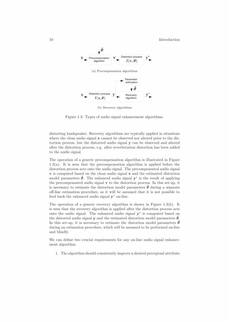
Figure 1.3: Types of audio signal enhancement algorithms.
distorting loudspeaker. Recovery algorithms are typically applied in situationswhere the clean audio signal x cannot be observed nor altered prior to the dis-tortion process, but the distorted audio signal y can be observed and alteredafter the distortion process, e.g. after reverberation distortion has been addedto the audio signal.
The operation of a generic precompensation algorithm is illustrated in Figure1.3(a). It is seen that the precompensation algorithm is applied before thedistortion process acts onto the audio signal. The precompensated audio signalv is computed based on the clean audio signal x and the estimated distortionmodel parameters θ. The enhanced audio signal y∗ is the result of applyingthe precompensated audio signal v to the distortion process. In this set-up, itis necessary to estimate the distortion model parameters θ during a separateoff-line estimation procedure, as it will be assumed that it is not possible tofeed back the enhanced audio signal y∗ on-line.
The operation of a generic recovery algorithm is shown in Figure 1.3(b). Itis seen that the recovery algorithm is applied after the distortion process actsonto the audio signal. The enhanced audio signal y∗ is computed based onthe distorted audio signal y and the estimated distortion model parameters θ.In this set-up, it is necessary to estimate the distortion model parameters θduring an estimation procedure, which will be assumed to be performed on-lineand blindly.
We can define two crucial requirements for any on-line audio signal enhance-ment algorithm:
1. The algorithm should consistently improve a desired perceptual attribute

1.2. Precompensation Algorithms 11
(audio quality, speech quality, speech intelligibility), i.e. the perceptualattribute should be better for the enhanced audio signal y∗ comparedto the distorted audio signal y. Ideally, the enhanced audio signal y∗ isequal to the clean audio signal x.
2. The algorithm should be able to run under strict constraints regardingcomputation time, resource usage and power consumption, as will betypically imposed by (mobile) audio devices.
In the next sections, we will discuss the state of the art and the prevailingchallenges for precompensation algorithms (see Section 1.2) and recovery al-gorithms (see Section 1.3). For both types of audio signal enhancement algo-rithms, the analysis will focus on two commonly encountered yet challengingaudio signal distortion processes. In Section 1.4, we will outline a novel audiosignal enhancement framework for overcoming the limitations of existing audiosignal enhancement algorithms, which is based on the application of embeddedoptimization and perceptual models.
1.2 Precompensation Algorithms
From Figure 1.3(a), we can define the following steps in the operation of ageneric precompensation algorithm:
1. Off-line selection of a suitable distortion model f(v, θ).2. Off-line estimation of distortion model parameters θ.3. On-line computation of precompensated audio signal v.
We will now review the problem statement and state of the art of precompen-sation algorithms for mitigating hard clipping distortion (subsection 1.2.1) andloudspeaker distortion (subsection 1.2.2), thereby focusing on the efficiency andlimitations in performing the three steps mentioned above.
1.2.1 Hard Clipping Precompensation
Hard clipping is a nonlinear distortion process commonly encountered in audioapplications, and can occur during the recording, mastering, storage, trans-mission and reproduction stages of the audio signal path. When hard clippingoccurs, the amplitude of the clean audio signal is cut off such that no sampleamplitude exceeds a given amplitude range [L,U ]. This introduces differentkinds of unwanted nonlinear distortion into the audio signal such as odd har-monic distortion, intermodulation distortion and aliasing distortion [34]. In aseries of listening experiments performed on normal hearing listeners [2] andhearing-impaired listeners [35], it was concluded that the application of hardclipping to audio signals has a significant negative effect on perceived audio

12 Introduction
quality scores, irrespective of the subject’s hearing acuity. Moreover, it wasconcluded that hard clipping distortion reduces speech intelligibility, both fornormal-hearing and hearing-impaired listeners [31]. Hard clipping precompen-sation algorithms typically focus on reducing the negative effects of hard clip-ping on the resulting audio quality. The operation of a generic hard clippingprecompensation algorithm is shown in Figure 1.4.
Distortion Model Selection
The selection of a suitable distortion model is straightforward in this case. Asshown in Figure 1.4, the hard clipping distortion can be exactly modeled usinga memoryless hard clipping nonlinearity that is linear in the amplitude range[L,U ], and abruptly saturates when exceeding this amplitude range.
Distortion Model Parameter Estimation
The parameters of the distortion model are the lower clipping level L < 0 andthe upper clipping level U > 0 of the memoryless nonlinearity. A commonapproach to estimate L and U is to detect the occurrence of hard clippingbased on the distorted audio signal. Such non-intrusive hard clipping detectionmethods rely on the inspection of anomalities in the amplitude histogram [36]in order to detect the occurrence of hard clipping and estimate the associatedparameters L and U . These methods are very accurate if the detection workson the raw hard clipped audio signal, but are less accurate when the hardclipped audio signal was perceptually encoded prior to detection, in which caserobust detection methods are necessary [37].
Precompensation Operation
Hard clipping precompensation algorithms aim to preventively limit the digitalaudio signal with respect to the estimated allowable amplitude range [L,U ] ofthe subsequent hard clipping distortion process. Ideally, the precompensatedaudio signal v can then pass through the hard clipping distortion process with-out being altered, i.e. y∗ = v. The precompensation algorithm is obviouslyexpected to add minimal distortion to the clean audio signal x. We can classifyexisting hard clipping precompensation algorithms into limiting algorithms andsoft clipping algorithms.
Limiting algorithms (or limiters) aim to provide control over the amplitudepeaks exceeding [L,U ] in the clean audio signal x, while changing the dynamicsand frequency content of the audio signal as little as possible [1]. Limiters areessentially amplifiers with a time-varying gain that is automatically controlledby the measured peak level of the clean audio signal x. The attack time andrelease time parameters specify how fast the gain is changed according to mea-

1.2. Precompensation Algorithms 13
Figure 1.4: Hard clipping precompensation.
sured peaks in the clean audio signal x. The attack time parameter defines howfast the gain is decreased when the input signal level rapidly increases, whilethe release time parameter defines how fast the gain is restored to its originalvalue when the input signal level rapidly decreases [38]. The setting of theseparameters entails a trade-off between distortion avoidance and peak limitingperformance, as the gain should be as smooth as possible for not having audibleartefacts, yet at the same time it should vary fast enough to suppress signalpeaks [39][40].
Soft clipping algorithms instantaneously limit the clean audio signal x to theestimated allowable amplitude range [L,U ] by applying a soft memoryless non-linearity, i.e. one having a gradual transition from the linear zone to the nonlin-ear zone. In fact, soft clipping algorithms are related to limiting algorithms inthat they can be viewed as limiters having an infinitely small attack and releasetime [1]. In general, soft memoryless nonlinearities introduce less perceptibleartefacts as compared to hard memoryless nonlinearities, because of the lowerlevel of the introduced harmonic distortion and aliasing distortion [41]. Nu-merous soft memoryless nonlinearities have been proposed, such as hyperbolictangent, inverse square root, parabolic sigmoid, cubic sigmoid, sinusoidal, andexponential soft memoryless nonlinearities [42][43].
While both limiting algorithms and soft clipping algorithms have been shownto work fairly well for mitigating the effects of specific hard clipping distortionprocesses, several limitations of these approaches can be indicated. Firstly,these algorithms are governed by a set of tunable parameters, such as theattack time and release time for limiting approaches, and the shape parametersof the applied soft memoryless nonlinearity in soft clipping approaches. Therelation between the parameter settings and the resulting enhancement of thedesired perceptual attribute is generally unclear, leading in many cases to anad hoc and trial-and-error based parameter tuning procedure. Secondly, asthese approaches act directly on the amplitude of the clean time-domain audiosignal, it is difficult to adapt to time-varying frequency characteristics of theclean audio signal. Lastly, as the properties of human sound perception are notincorporated into these approaches, it is not possible to focus on enhancing a

14 Introduction
Figure 1.5: Loudspeaker precompensation.
given perceptual attribute of the audio signal.
1.2.2 Loudspeaker Precompensation
Loudspeaker distortion is a form of combined linear and nonlinear distortionincurred when an audio signal is reproduced through a loudspeaker systemhaving a non-ideal response. At low amplitudes, the loudspeaker behaviour isalmost linear and nonlinear signal distortion is negligible. However, at higheramplitudes nonlinear distortion occurs, and is notably prominent in small andlow-cost loudspeakers, which are ubiquitous in mobile devices [44]. Linearloudspeaker distortion is typically perceived as affecting timbre or tone qual-ity, whereas nonlinear loudspeaker distortion is typically perceived as addingharshness or noisiness, or as the perception of crackles or clicks. The presenceof linear and nonlinear loudspeaker distortion has been found to result in asignificant degradation of the perceived audio quality, both when present sep-arately [2] and simultaneously [27]. Loudspeaker precompensation algorithmstypically focus on reducing the negative effects of loudspeaker distortion on theresulting audio quality.
Distortion Model Selection
The selection of a suitable model accurately representing the linear and non-linear loudspeaker distortion is not a trivial task. Loudspeaker models canbe classified as linear loudspeaker models or nonlinear loudspeaker models.Knowledge of the physical nonlinear mechanisms inside the loudspeaker canbe incorporated to different degrees, leading to a further subclassification inwhite-box, grey-box or black-box nonlinear loudspeaker models [45].
Traditionally, loudspeakers have been modeled using linear systems, such asFIR filters [46] and IIR filters [47]. Warped FIR and IIR filters [48], as well asKautz filters [49] have been proposed in order to allow for a better frequencyresolution allocation, radically reducing the required filter order.
Nonlinear loudspeaker behaviour can be taken into consideration by using non-linear loudspeaker models. The most widely used white-box nonlinear loud-
1.2. Precompensation Algorithms 15
speaker models are physical low-frequency lumped parameter models, whichtake into account nonlinearities in the motor part and the mechanical part ofthe loudspeaker [50]. Given the relative complexity of such physical loudspeakermodels and their limitation to low frequencies and low-order nonlinearities,simpler and more efficient grey-box nonlinear loudspeaker models have beenproposed, such as Hammerstein models [51], cascades of Hammerstein models[52], and Wiener models [53]. These models are composed of a linear dynamicpart and a nonlinear static part, capable of incorporating prior informationon the linear and nonlinear distortion mechanisms in the loudspeaker. Black-box models have also been applied to loudspeaker modeling, e.g. time-domainNARMAX models [54], or frequency-domain Volterra models [55]. A majordrawback of Volterra models is that the number of parameters grows exponen-tially with the model order, in contrast to Hammerstein and Wiener models.
Distortion Model Parameter Estimation
As shown in Figure 1.5, the loudspeaker model parameters can in general bedivided into a set of model parameters θL related to the linear part of themodel and a set of model parameters θNL related to the nonlinear part of themodel. For linear loudspeaker models, only the parameter set θL has to beestimated. For nonlinear loudspeaker models, both the parameter sets θL andθNL have to be estimated.
The parameters of linear loudspeaker models, grey-box and black-box nonlin-ear loudspeaker models are mostly estimated by exciting the loudspeaker withaudio-like signals, e.g. random phase multisines [56], and recording the repro-duced signal. The parameters of white-box low-frequency lumped parametermodels can be estimated by exciting the loudspeaker with an audio-like signaland measuring the voice coil current [15], or the voice coil displacement usingan optical sensor [57].
While the parameter estimation of linear loudspeaker models can be performedusing standard linear identification methods, the parameter estimation of non-linear loudspeaker models is a challenging problem. Hammerstein model pa-rameter estimation requires the solution of a bi-convex optimization problem,having an objective function featuring cross products between parameters inθL and parameters in θNL. Techniques2 to solve this bi-convex optimizationproblem include the iterative approach [59], the overparametrization approach[60], and the subspace approach [61]. Wiener model parameter estimationmethods have been derived along the lines of their Hammerstein counterparts,resulting in the same categories of approaches for solving the bi-convex op-timization problem [62]. Volterra model parameters can be estimated usingadaptive algorithms such as NLMS [55].
2A nice overview of different Hammerstein model identification methods is given in [58].

16 Introduction
Precompensation Operation
The operation of a generic loudspeaker precompensation algorithm is shownin Figure 1.5. The idea is to reduce the linear and nonlinear distortion ef-fects caused by the loudspeaker, by applying a precompensation step to theclean audio signal x before feeding it to the loudspeaker input. The estimatedloudspeaker model parameters θL and θNL are used in the precompensation.
When using linear loudspeaker models, precompensation consists in performinglinear equalization of the loudspeaker by computing (based on θL) and apply-ing an inverse digital filter to the audio signal. An ideal linear equalizationwould result in a reproduction channel having a flat frequency response and aconstant group delay. Among the proposed equalization approaches, we men-tion the distinction between direct inversion and indirect inversion approaches,and between minimum-phase and nonminimum-phase designs. In general, theperformance of these equalization approaches is seen to largely depend on thestationarity and the accuracy of the loudspeaker models [49].
When using nonlinear loudspeaker models, precompensation consists in per-forming either linearization or full equalization of the loudspeaker. The aimof linearization is to make the reproduction channel a linear system, therebycompensating for the nonlinear distortion in the loudspeaker [63]. The aimof full equalization is to make the reproduction channel transparent, therebycompensating for both the linear and nonlinear distortion in the loudspeaker.
Nonlinear loudspeaker precompensation methods for performing linearizationhave been proposed for white-box, grey-box and black-box loudspeaker models.For white-box low-frequency lumped parameter models, seminal linearizationmethods are based on the application of nonlinear inversion [50] and a mirrorfilter [64]. A control-theoretic feedback linearization approach was theoreti-cally shown to allow for exact linearization under certain assumptions [65], andthis approach was modified to achieve a satisfactory approximate linearizationin practice [66]. For grey-box Wiener and Hammerstein loudspeaker models,linearization methods have been proposed based on the coherence criterion [51]and polynomial root finding [67]. For black-box Volterra loudspeaker models,a p-th order inverse model was succesfully applied to achieve loudspeaker lin-earization [68]. The main disadvantage of these methods resides in their highcomputational complexity.
Nonlinear loudspeaker precompensation methods for performing full equaliza-tion rely on the computation of an inverse nonlinear loudspeaker model. How-ever, the exact inverse of the nonlinear loudspeaker model only exists in spe-cific cases. For Hammerstein and Wiener loudspeaker models, an exact inverseonly exists if the inverse of the static nonlinearity exists. Volterra loudspeakermodels in general do not allow for computing an exact inverse model. As aconsequence, practical full equalization methods rely on the computation of an
1.3. Recovery Algorithms 17
inexact inverse model, which brings along problems with both the stability andthe computational complexity of these methods [44].
In conlusion, several general limitations of the existing approaches for loud-speaker precompensation can be indicated. Firstly, their fairly high computa-tional complexity conflicts with the requirement to perform loudspeaker com-pensation in real time on mobile audio devices. Secondly, as the properties ofhuman sound perception are not incorporated into these approaches, it is notpossible to focus on enhancing a given perceptual attribute of the audio signal.
1.3 Recovery Algorithms
From Figure 1.3(b), we can define the following steps in the operation of ageneric recovery algorithm:
1. Off-line selection of a suitable distortion model f(x, θ).2. On-line blind estimation of distortion model parameters θ.3. On-line computation of the enhanced audio signal y∗.
We will now review the problem statement and state-of-the-art of recoveryalgorithms for enhancing audio signals degraded by hard clipping distortion(subsection 1.3.1) and reverberation distortion (subsection 1.3.2), thereby fo-cusing on the efficiency and limitations in performing the three steps mentionedabove.
1.3.1 Declipping
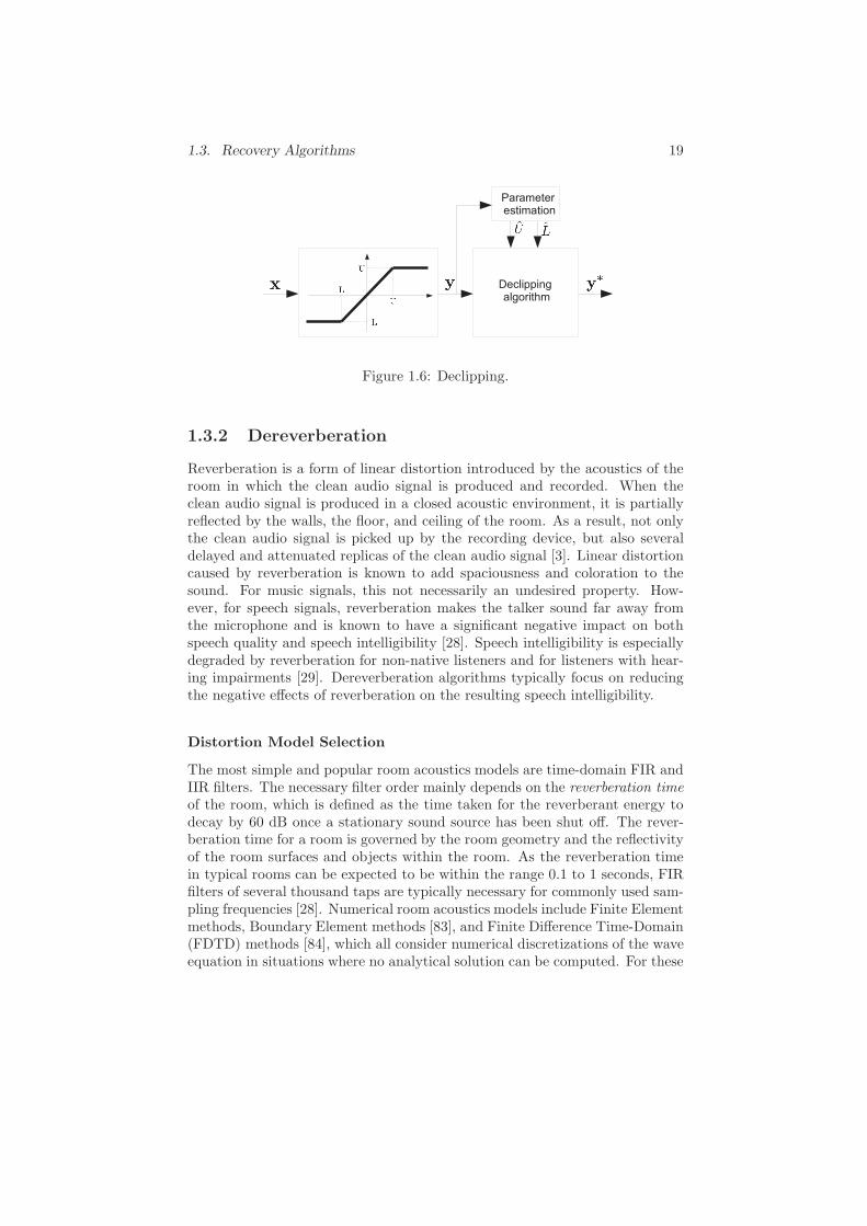
In subsection 1.2.1, it was shown that hard clipping is a nonlinear distortionprocess that can occur in almost any stage of the audio signal path, and hasa significant negative effect on the audio quality, speech quality and speechintelligiblity. In situations where hard clipping can not be anticipated for, onehas to perform declipping, i.e. the recovery of the clean audio signal x basedon the hard clipped audio signal y. The operation of a generic declippingalgorithm is shown in Figure 1.6.
Distortion Model Selection and Parameter Estimation
As mentioned in subsection 1.2.1, the selection of a suitable distortion modelis straightforward, i.e. the hard clipping distortion can be exactly modeledusing a memoryless hard clipping nonlinearity that is linear in the amplituderange [L,U ], and abruptly saturates when exceeding this amplitude range. Theparameters of the distortion model are the lower clipping level L < 0 and theupper clipping level U > 0 of the memoryless nonlinearity. These parameters
18 Introduction
can be estimated based on the hard clipped audio signal y, using histogrammethods.
Recovery Operation
Several approaches to the declipping problem have been proposed. A firstapproach is based on performing an interpolation procedure to recover theclipped signal samples based on the knowledge of the unclipped signal sam-ples. Interpolation algorithms differ in particular in the a priori knowledge andassumptions on the clean audio signal x that are incorporated into the inter-polation procedure. Autoregressive [69], sinusoidal [70] and statistical audiosignal models [71] have been used, as well as restrictions on the spectral enve-lope [72], bandwidth [73], and time-domain amplitude [71][73][74] of the cleanaudio signal. A second approach tackles the declipping problem as a supervisedlearning problem, in which the temporal and spectral properties of clean andclipped audio signals are learned through an artificial neural network [75], or aHidden Markov Model (HMM) [76].
The third and most recent approach addresses the declipping problem in theframework of compressed sensing (CS). In the CS framework, declipping isformulated and solved as a sparse signal recovery problem, where one takesadvantage of the sparsity of the clean audio signal (in some basis or dictionary)in order to recover it from a subset of its samples. Sparse signal recovery meth-ods for declipping differ in the sparsifying basis or dictionary that is used torepresent the clean audio signal, and in the optimization procedure that is usedfor computing the recovered audio signal. Commonly used sparse audio signalrepresentations include the Discrete Fourier Transform (DFT) basis [77], theovercomplete Discrete Fourier Transform (DCT) dictionary [78][79], and theovercomplete Gabor dictionary [80]. In order to solve the sparse signal recov-ery optimization problem, existing algorithms such as Orthogonal MatchingPursuit (OMP) [78], Iterative Hard Thresholding (IHT) [79], Trivial Pursuit(TP) [77] and reweighted L1-minimization [77] have been adapted in order toincorporate constraints specific to the declipping problem. For some of thesesparse signal recovery methods for declipping, deterministic recovery guaran-tees have been derived in [81][82].
In conclusion, we can point out a general limitation of the existing declippingmethods. Whereas all these methods do include a model of the clean audiosignal, they do not incorporate a model of the human sound perception, makingit impossible to focus on enhancing a given perceptual attribute of the audiosignal.
1.3. Recovery Algorithms 19
Figure 1.6: Declipping.
1.3.2 Dereverberation
Reverberation is a form of linear distortion introduced by the acoustics of theroom in which the clean audio signal is produced and recorded. When theclean audio signal is produced in a closed acoustic environment, it is partiallyreflected by the walls, the floor, and ceiling of the room. As a result, not onlythe clean audio signal is picked up by the recording device, but also severaldelayed and attenuated replicas of the clean audio signal [3]. Linear distortioncaused by reverberation is known to add spaciousness and coloration to thesound. For music signals, this not necessarily an undesired property. How-ever, for speech signals, reverberation makes the talker sound far away fromthe microphone and is known to have a significant negative impact on bothspeech quality and speech intelligibility [28]. Speech intelligibility is especiallydegraded by reverberation for non-native listeners and for listeners with hear-ing impairments [29]. Dereverberation algorithms typically focus on reducingthe negative effects of reverberation on the resulting speech intelligibility.
Distortion Model Selection
The most simple and popular room acoustics models are time-domain FIR andIIR filters. The necessary filter order mainly depends on the reverberation timeof the room, which is defined as the time taken for the reverberant energy todecay by 60 dB once a stationary sound source has been shut off. The rever-beration time for a room is governed by the room geometry and the reflectivityof the room surfaces and objects within the room. As the reverberation timein typical rooms can be expected to be within the range 0.1 to 1 seconds, FIRfilters of several thousand taps are typically necessary for commonly used sam-pling frequencies [28]. Numerical room acoustics models include Finite Elementmethods, Boundary Element methods [83], and Finite Difference Time-Domain(FDTD) methods [84], which all consider numerical discretizations of the waveequation in situations where no analytical solution can be computed. For these
20 Introduction
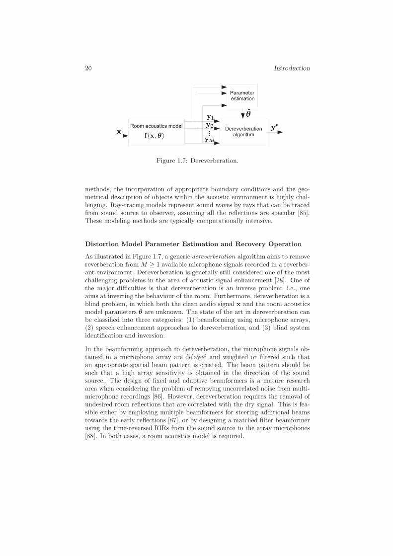
Figure 1.7: Dereverberation.
methods, the incorporation of appropriate boundary conditions and the geo-metrical description of objects within the acoustic environment is highly chal-lenging. Ray-tracing models represent sound waves by rays that can be tracedfrom sound source to observer, assuming all the reflections are specular [85].These modeling methods are typically computationally intensive.
Distortion Model Parameter Estimation and Recovery Operation
As illustrated in Figure 1.7, a generic dereverberation algorithm aims to removereverberation fromM ≥ 1 available microphone signals recorded in a reverber-ant environment. Dereverberation is generally still considered one of the mostchallenging problems in the area of acoustic signal enhancement [28]. One ofthe major difficulties is that dereverberation is an inverse problem, i.e., oneaims at inverting the behaviour of the room. Furthermore, dereverberation is ablind problem, in which both the clean audio signal x and the room acousticsmodel parameters θ are unknown. The state of the art in dereverberation canbe classified into three categories: (1) beamforming using microphone arrays,(2) speech enhancement approaches to dereverberation, and (3) blind systemidentification and inversion.
In the beamforming approach to dereverberation, the microphone signals ob-tained in a microphone array are delayed and weighted or filtered such thatan appropriate spatial beam pattern is created. The beam pattern should besuch that a high array sensitivity is obtained in the direction of the soundsource. The design of fixed and adaptive beamformers is a mature researcharea when considering the problem of removing uncorrelated noise from multi-microphone recordings [86]. However, dereverberation requires the removal ofundesired room reflections that are correlated with the dry signal. This is fea-sible either by employing multiple beamformers for steering additional beamstowards the early reflections [87], or by designing a matched filter beamformerusing the time-reversed RIRs from the sound source to the array microphones[88]. In both cases, a room acoustics model is required.
1.4. Embedded Optimization Framework for Audio Signal Enhancement 21
Several speech enhancement approaches to dereverberation have been explored.An early approach was shown to be capable of compensating for early reflec-tions in the cepstral domain [89]. A more successful technique is based on linearprediction [90], and exploits the observation that reverberation only alters thelinear prediction (LP) residual of a speech signal, but not the autoregressive(AR) coefficients. Dereverberated speech can then be synthesized from the ARcoefficients, using an enhanced LP residual signal obtained through matchedfiltering [91], kurtosis maximization [92], or spatiotemporal averaging [93]. An-other speech enhancement approach to dereverberation is spectral subtraction,which can be applied in a single-channel [94] or multi-channel [95] scenario.Again, a room acoustics model is necessary for being able to estimate and sub-tract the spectral contribution of reverberation from the microphone signals.
A promising yet challenging approach to dereverberation is blind system iden-tification and inversion. The aim is to identify the room acoustics model fromthe observed microphone signals, to invert this model, and to process the micro-phone signals with the inverse model to obtain an estimate of the clean audiosignal. In a multi-channel scenario, the blind system identification problem canbe elegantly formulated as an eigenvalue problem, for which least-squares [96],subspace [97], and adaptive filtering [98] solutions have been proposed. How-ever, the application of these algorithms to blind identification of room acous-tics was found to be nontrivial due to nonstationarity, robustness, and compu-tational issues [28]. The inversion of the identified room acoustics model canbe performed in a single-channel scenario [99], although multi-channel channelinversion was found to be computationally more promising and more appealing[100]. More recently, subband [101] and adaptive [102] implementations formulti-channel inversion have been proposed, as well as regularized algorithmsto improve robustness against model identification errors [32][103][104].
1.4 Embedded Optimization Framework for Per-
ceptual Audio Signal Enhancement
From the overview of the state-of-the-art algorithms for hard clipping precom-pensation, loudspeaker precompensation, declipping and dereverberation, wecan point out two major general limitations of existing audio signal enhance-ment algorithms:
• The properties of human sound perception are most often not incorpo-rated into traditional audio signal enhancement algorithms. As a result,the relation between the algorithm parameters and the perceptual at-tribute to enhance is not clearly defined, nor can it be ensured that thedesired perceptual attribute will indeed be enhanced.
• Most traditional audio signal enhancement algorithms rely on a sequence

22 Introduction
of a (non)linear system identification, the inversion of the identified sys-tem, and the application of the inverted system to the audio signal.This sequence is mostly computationally intensive and often containsill-conditioned steps.
The goal of this thesis is to overcome the limitations of existing audio signalenhancement approaches, by exploring a new audio signal enhancement frame-work. In this embedded optimization framework, the audio signal enhancementproblem at hand is reformulated as a per-frame numerical optimization prob-lem, aimed at enhancing a desired perceptual attribute.
1.4.1 Embedded Optimization
Traditionally, numerical optimization has been applied in speech and audiosignal processing applications for tasks such as FIR filter and filterbank de-sign [105], microphone array weight design [106], and feature learning in audioclassification [107] or speech recognition [108]. These design tasks are typicallyperformed off-line, and the optimization is carried out on time scales of seconds,minutes or hours, often without strict computation time constraints. Recently,the growing computational power and algorithmic developments have openedup the possibility of embedding numerical optimization directly into real-timesignal processing algorithms in order to carry out nonlinear processing on thesignal itself. In this embedded optimization paradigm, the optimization vari-ables are signal samples instead of filter weights or model parameter values,and the optimization can be performed on-line with strict computation timeconstraints, on time scales as short as milliseconds or microseconds [109].
This thesis investigates the development of an embedded optimization frame-work for audio signal enhancement, and its application to both precompensa-tion algorithms and recovery algorithms. In Figure 1.8(a), the concept of anembedded optimization algorithm for the precompensation of audio signals isvisualized. The algorithm operates on short-time clean audio signal frames xm
of N samples, where m denotes the frame index. The precompensated audiosignal frame vm is computed by solving a per-frame constrained optimizationproblem of the following form:
minimizevm∈RN
dm(xm, y∗m) subject to y∗
m = f(vm, θm) (1.1)
where a given distance measure dm between the clean audio signal frame xm andthe predicted enhanced audio signal frame y∗
m is minimized, and the constraintsmodel the subsequent distortion process using distortion model parameters θmderived from an off-line estimation procedure. In Figure 1.8(b), the conceptof an embedded optimization algorithm for the recovery of audio signals isvisualized. The enhanced audio signal frame y∗
m is computed by solving a
1.4. Embedded Optimization Framework for Audio Signal Enhancement 23
per-frame constrained optimization problem of the following form:
minimizey∗
m∈RNdm(y∗
m) subject to ym = f(y∗m, θm) (1.2)
where a given measure dm of the enhanced audio signal frame y∗m is minimized,
and the constraints model the preceding distortion process using distortionmodel parameters θm derived from an on-line estimation procedure.
The embedded optimization framework allows us to compute in real time anenhanced audio signal frame y∗
m that is optimal according to any desired math-ematical measure dm. For audio signal enchancement applications, the mostrelevant measure to minimize is the perceived degradation of a selected percep-tual attribute (e.g. audio quality, speech quality, speech intelligibility) betweenthe clean audio signal frame xm and the enhanced signal frame y∗
m. The trans-lation from the subjective perceptual attribute degradation to the objectivemathematical measure dm can be performed using a suitable model of humansound perception, as will be discussed next.
1.4.2 Perceptual Models
The human perception of sounds is a complex process involving both auditoryand cognitive mechanisms. In the last decades, considerable research effortshave been spent in order to thoroughly understand and accurately model theessential properties of human sound perception. As giving a complete overviewof these findings is largely beyond the scope of this thesis, we will focus onpointing out a few properties of the human perception of sounds which aremost relevant to the perception of linear and nonlinear distortion.
Most important, the sensitivity of the human hearing system is dependent onthe frequency of the tone. This effect is characterized by the absolute thresholdof hearing, which is defined as the required Sound Pressure Level (SPL) of apure tone such that an average listener will just hear the tone in a noiselessenvironment. The absolute threshold of hearing has been measured experimen-tally [110] and is depicted as the solid line in Figure 1.9. It is seen that thehuman hearing system is most sensitive in the middle part of the frequencyrange, and less sensitive for the lower and upper parts of the frequency range.Whenever two or more tones are simultaneously presented to the human hear-ing system, the phenomenon of simultaneous masking may occur, where thepresence of one stronger tone (the masker) renders imperceptible the simul-taneous presence of a weaker tone (the maskee) at a nearby frequency [111].In Figure 1.9, the strong masker tone is seen to push the absolute treshold ofhearing upwards for nearby frequencies, resulting in a masking treshold (dot-ted line), i.e. the required SPL of a tone such that an average listener will justhear the tone in the simultaneous presence of the masker. As the two displayedtones at nearby frequencies are situated below the masking threshold, they willbe imperceptible in the simultaneous presence of the masker.

24 Introduction
(a) Precompensation algorithm
(b) Recovery algorithm
Figure 1.8: Embedded optimization algorithms for perceptual audio signal en-hancement.
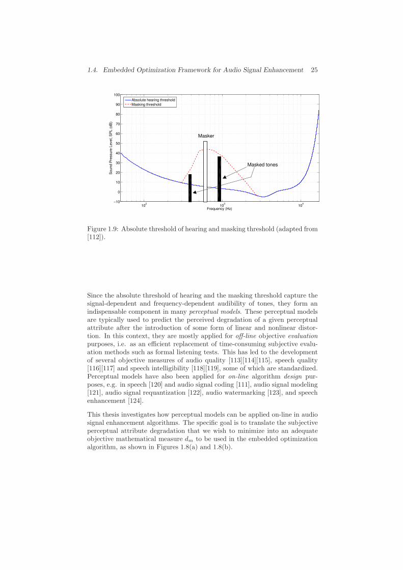
1.4. Embedded Optimization Framework for Audio Signal Enhancement 25
102
103
104
−10
0
10
20
30
40
50
60
70
80
90
100
Frequency (Hz)
So
un
d P
ressu
re L
eve
l, S
PL
(d
B)
Absolute hearing threshold
Masking threshold
Masked tones
Masker
Figure 1.9: Absolute threshold of hearing and masking threshold (adapted from[112]).
Since the absolute threshold of hearing and the masking threshold capture thesignal-dependent and frequency-dependent audibility of tones, they form anindispensable component in many perceptual models. These perceptual modelsare typically used to predict the perceived degradation of a given perceptualattribute after the introduction of some form of linear and nonlinear distor-tion. In this context, they are mostly applied for off-line objective evaluationpurposes, i.e. as an efficient replacement of time-consuming subjective evalu-ation methods such as formal listening tests. This has led to the developmentof several objective measures of audio quality [113][114][115], speech quality[116][117] and speech intelligibility [118][119], some of which are standardized.Perceptual models have also been applied for on-line algorithm design pur-poses, e.g. in speech [120] and audio signal coding [111], audio signal modeling[121], audio signal requantization [122], audio watermarking [123], and speechenhancement [124].
This thesis investigates how perceptual models can be applied on-line in audiosignal enhancement algorithms. The specific goal is to translate the subjectiveperceptual attribute degradation that we wish to minimize into an adequateobjective mathematical measure dm to be used in the embedded optimizationalgorithm, as shown in Figures 1.8(a) and 1.8(b).

26 Introduction
1.4.3 Main Research Objectives
The main research objectives of this thesis can be stated as follows:
1. Development of an embedded optimization framework for audio signal en-hancement, resulting in improved audio signal enhancement algorithmsfor the precompensation and recovery of audio signals subject to dif-ferent types of linear and nonlinear audio signal distortion. Specificalgorithms for hard clipping precompensation, loudspeaker precompen-sation, declipping and dereverberation are targeted.
2. Incorporation of perceptual models in the embedded optimization frame-work, in order to allow for the consistent enhancement of desired per-ceptual attributes. The targeted perceptual attribute in this thesis isperceived audio quality.
3. Design of application-tailored optimization methods and their efficienthardware implementation in order to solve the per-frame optimizationproblems under strict constraints regarding computation time, resourceusage and power consumption.
4. Comparative objective and subjective evaluation between the developedembedded optimization algorithms and state-of-the-art audio signal en-hancement algorithms.
.
1.5 Thesis Outline and Publications
1.5.1 Chapter-By-Chapter Outline and Contributions
Chapter 2 tackles the problem of hard clipping precompensation using an em-bedded optimization approach, aimed at minimizing the perceptible nonlinearaudio signal distortion. First, the subjective notion of perceptible nonlineardistortion is translated into a mathematical measure by including frequencyweights based on the instantaneous masking threshold, which is computed us-ing a perceptual model. Then, hard clipping precompensation is formulatedas a sequence of per-frame constrained convex quadratic optimization prob-lems. Next, three different structure-exploiting convex optimization methodsare proposed for solving the per-frame optimization problems in a fast and re-liable way, and their corresponding theoretical complexity bounds are derived.The fastest of these methods is an optimal projected gradient method, which isshown to run in real time on a standard PC. Finally, a comparative objectiveevaluation reports significantly higher objective audio quality scores using the

1.5. Thesis Outline and Publications 27
embedded optimization algorithm over standard hard clipping precompensa-tion techniques, and this for moderate to high levels of clipping.
Chapter 3 focuses on the problem of loudspeaker precompensation, in whichthe aim is to minimize the combined perceptible linear and nonlinear audiosignal distortion incurred in the loudspeaker, again by using an embedded opti-mization approach. The loudspeaker is modeled using a grey-box Hammersteinloudspeaker model, i.e. a cascade of a memoryless nonlinearity and a linear FIRfilter. First, the subjective notion of perceptible linear and nonlinear distortionis translated into a mathematical measure by including frequency weights basedon the instantaneous masking threshold in a similar fashion as in Chapter 2.Then, loudspeaker precompensation is formulated as a sequence of per-framenonconvex optimization problems. Next, the resulting per-frame optimizationproblems are solved efficiently using first-order optimization methods. Depend-ing on the invertibility and the smoothness of the memoryless nonlinearity inthe Hammerstein loudspeaker model, different first-order optimization methodsare proposed and their convergence properties are analyzed. Finally, objectiveevaluation experiments using synthetic and identified loudspeaker models showthat the embedded optimization loudspeaker precompensation algorithm pro-vides a significant audio quality improvement, especially so at high loudspeakerplayback levels.
Chapter 4 reports the set-up and results of subjective evaluation experimentsfor the hard clipping precompensation algorithms of Chapter 2 and the loud-speaker precompensation algorithms of Chapter 3. The subjective evaluationtakes the form of a formal listening test including 19 test subjects, each of whichis asked to quantify the perceived audio quality of audio signals processed bythe different precompensation algorithms. Statistical hypothesis tests on theobtained subject responses lead to the following conclusions. Firstly, the per-ceived audio quality of audio signals processed by the embedded optimizationclipping precompensation algorithm of Chapter 2 is significantly superior tothat of audio signals processed by an existing clipping precompensation algo-rithm. Secondly, the perceived audio quality of audio signals processed by theembedded optimization loudspeaker precompensation algorithm of Chapter3 before being fed into the Hammerstein loudspeaker model is significantlysuperior to that of audio signals not processed before being fed into the Ham-merstein loudspeaker model, and this for moderate to high amplitude levels.Thirdly, there is no reason to believe that the perceived audio quality of audiosignals subject to a certain nonlinear hard clipping distortion would be supe-rior to that of audio signals subject to a combination of the same nonlinearhard clipping distortion and an additional linear distortion. Lastly, there isa significant positive correlation between subjective audio quality scores andobjective audio quality scores.
Chapter 5 considers the hardware implementation on a field programmablegate array (FPGA) of the optimal projected gradient method proposed in
28 Introduction
Chapter 2 for solving the per-frame convex optimization problems. A cou-ple of organizational changes are proposed in the optimal projected gradientmethod in order to allow for an efficient FPGA implementation architecture.The architecture selection for implementing the Fast Fourier Transform (FFT)is seen to entail a trade-off between resource usage and throughput. By per-forming bit-accurate simulations of the FPGA implementation, it is demon-strated that the choice between fixed-point arithmetic and floating-point arith-metic and the selection of the corresponding bit width has an impact on theresulting audio quality as well as on the resource usage and power consumptionof the design. The selected FPGA design, which performs 30 optimal projectedgradient iterations using 20 fixed-point fraction bits, has a low latency, a re-duced power consumption, a reduced resource usage, and at the same timepreserves the full audio quality improvement. This design allows to performthe algorithm in real time on a small and portable device.
Chapter 6 focuses on the problem of declipping, i.e. the recovery of audio sig-nals degraded by nonlinear hard clipping distortion. An embedded optimiza-tion algorithm for declipping is proposed that is jointly based on the theory ofcompressed sensing (CS) and on properties of human auditory perception. De-clipping is formulated as a sparse signal recovery problem in the DFT domain,in which the recovery is performed by solving a per-frame ℓ1-norm-type opti-mization problem. The optimization problem formulation differs from existingCS-based declipping formulations in the inclusion of frequency weights in theℓ1-norm, based on the instantaneous masking threshold. As a result, the de-clipping algorithm is focused on maximizing the perceived audio quality of thedeclipped signal instead of the physical signal reconstruction quality. Compar-ative objective and subjective evaluation experiments reveal a significant audioquality increase for the proposed embedded optimization declipping algorithmcompared to existing CS-based declipping algorithms.
Chapter 7 focuses on the problem of multi-microphone dereverberation, wherethe aim is to eliminate linear reverberation distortion introduced by the acous-tics of the room in which the clean audio signal is recorded. An embedded opti-mization approach to multi-microphone dereverberation is proposed, allowingfor a joint estimation of the room acoustics model parameters and the cleanaudio signal. The proposed approach differs from existing blind system identi-fication and inversion approaches in that it does not require an explicit systeminversion. It is shown how the inherently nonconvex joint estimation problemcan be smoothed by including regularization terms based on a statistical latereverberation model and a sparsity prior for the clean audio signal spectrum.Depending on the included regularization terms, one of three different sequen-tial optimization algorithms for solving the nonconvex optimization problem isapplied. A performance evaluation for an example multi-microphone derever-beration scenario shows promising results, thus motivating future research inthis direction.

1.5. Thesis Outline and Publications 29
Chapter 8 summarizes the main conclusions of the research presented in thisthesis, and points out suggestions for future research.
1.5.2 Included Publications
The following publications are included in this thesis:
Part II: Precompensation algorithms
Chapter 2: Hard Clipping PrecompensationB. Defraene, T. van Waterschoot, H.J. Ferreau, M. Diehl, and M. Moonen,“Real-time perception-based clipping of audio signals using convex optimiza-tion,” IEEE Trans. Audio Speech Language Process., vol. 20, no. 10, pp.2657–2671, Dec. 2012.
Chapter 3: Loudspeaker PrecompensationB. Defraene, T. van Waterschoot, M. Diehl, and M. Moonen, “Embedded-optimization-based loudspeaker compensation using a Hammerstein loud-speaker model,” IEEE Trans. Audio Speech Language Process., submittedfor publication, Nov. 2013.
Part III: Recovery algorithms
Chapter 6: Declipping Using Perceptual Compressed SensingB. Defraene, N. Mansour, S. De Hertogh, T. van Waterschoot, M. Diehl,and M. Moonen, “Declipping of audio signals using perceptual compressedsensing,” IEEE Trans. Audio Speech Language Process., vol. 21, no. 12, pp.2627-2637, Dec. 2013.
Chapter 7: Multi-Microphone DereverberationT. van Waterschoot, B. Defraene, M. Diehl, and M. Moonen, “EmbeddedOptimization Algorithms for Multi-Microphone Dereverberation,” in Proc.of the 21st European Signal Process. Conf. (EUSIPCO ’13), Marrakech,Morocco, Sept. 2013.
30 Bibliography
Bibliography
[1] U. Zolzer, X. Amatriain, and J. Wiley, DAFX: digital audio effects. Wi-ley Online Library, 2002, vol. 1.
[2] C.-T. Tan, B. C. Moore, and N. Zacharov, “The effect of nonlinear dis-tortion on the perceived quality of music and speech signals,” Journal ofthe Audio Engineering Society, vol. 51, no. 11, pp. 1012–1031, 2003.
[3] T. van Waterschoot, “Design and evaluation of digital signal processingalgorithms for acoustic feedback and echo cancellation,” Ph.D. disserta-tion, KU Leuven, Leuven, Belgium, Mar. 2009.
[4] U. Zolzer, Digital audio signal processing. Wiley. com, 2008.
[5] J. Eargle, The Microphone Book: From mono to stereo to surround-aguide to microphone design and application. Taylor & Francis US, 2004.
[6] B. Katz and R. A. Katz,Mastering audio: the art and the science. Taylor& Francis US, 2007.
[7] E. Vickers, “The loudness war: Background, speculation, and recommen-dations,” in Audio Engineering Society Convention 129. Audio Engi-neering Society, 2010.
[8] C.-M. Liu, H.-W. Hsu, and W.-C. Lee, “Compression artifacts in per-ceptual audio coding,” Audio, Speech, and Language Processing, IEEETransactions on, vol. 16, no. 4, pp. 681–695, 2008.
[9] A. Spanias, T. Painter, and V. Atti, Audio signal processing and coding.Wiley. com, 2006.
[10] K. C. Pohlmann, The compact disc: a handbook of theory and use. AREditions, Inc., 1989, vol. 5.
[11] S. Godsill, P. Rayner, and O. Cappe, “Digital audio restoration,” Appli-cations of digital signal processing to audio and acoustics, pp. 133–194,2002.
[12] M.-Y. Zhu, M. Zhang, X.-Q. Yu, and W.-G. Wan, “Streaming audiopacket loss concealment based on sinusoidal frequency estimation in mdctdomain,” Consumer Electronics, IEEE Transactions on, vol. 56, no. 2,pp. 811–819, 2010.
[13] S. Linkwitz, “Investigation of sound quality differences between monopo-lar and dipolar woofers in small rooms,” in Audio Engineering SocietyConvention 105. Audio Engineering Society, 1998.
31
[14] J. Borwick, Loudspeaker and headphone handbook. Taylor & Francis US,2001.
[15] W. Klippel, “Diagnosis and remedy of nonlinearities in electrodynami-cal transducers,” in Audio Engineering Society Convention 109. AudioEngineering Society, 2000.
[16] ——, “Tutorial: Loudspeaker nonlinearitiescauses, parameters, symp-toms,” Journal of the Audio Engineering Society, vol. 54, no. 10, pp.907–939, 2006.
[17] D. Kolossa and R. Haeb-Umbach, Robust speech recognition of uncertainor missing data: theory and applications. Springer, 2011.
[18] D. Fragoulis, G. Rousopoulos, T. Panagopoulos, C. Alexiou, and C. Pa-paodysseus, “On the automated recognition of seriously distorted musicalrecordings,” Signal Processing, IEEE Transactions on, vol. 49, no. 4, pp.898–908, 2001.
[19] A. Gabrielsson and H. Sjogren, “Perceived sound quality of sound-reproducing systems,” Journal of the Acoustical Society of America,vol. 65, no. 4, pp. 1019–1033, 1979.
[20] S. Bech and N. Zacharov, Perceptual audio evaluation-Theory, methodand application. Wiley. com, 2007.
[21] J. Benesty, M. M. Sondhi, and Y. Huang, Springer handbook of speechprocessing. Springer, 2008.
[22] M. Waltermann, A. Raake, and S. Moller, “Quality dimensions of nar-rowband and wideband speech transmission,” Acta Acustica united withAcustica, vol. 96, no. 6, pp. 1090–1103, 2010.
[23] N. Cote, T-Labs Series In Telecommunication Services: Integral and Di-agnostic Intrusive Prediction of Speech Quality. Springer, 2011, vol. 1.
[24] A. Raake, Speech Quality of VoIP: Assessment and Prediction. Wiley.com, 2007.
[25] B. C. Moore and C.-T. Tan, “Perceived naturalness of spectrally distortedspeech and music,” The Journal of the Acoustical Society of America, vol.114, p. 408, 2003.
[26] A. Gabrielsson, B. Hagerman, T. Bech-Kristensen, and G. Lundberg,“Perceived sound quality of reproductions with different frequency re-sponses and sound levels,” The Journal of the Acoustical Society of Amer-ica, vol. 88, p. 1359, 1990.

32 Bibliography
[27] B. C. Moore, C.-T. Tan, N. Zacharov, and V.-V. Mattila, “Measuring andpredicting the perceived quality of music and speech subjected to com-bined linear and nonlinear distortion,” Journal of the Audio EngineeringSociety, vol. 52, no. 12, pp. 1228–1244, 2004.
[28] P. A. Naylor and N. D. Gaubitch, Speech dereverberation. Springer,2010.
[29] E. A. P. Habets, “Single- and multi-microphone speech dereverberationusing spectral enhancement,” 2007.
[30] K. H. Arehart, J. M. Kates, M. C. Anderson, and L. O. Harvey Jr,“Effects of noise and distortion on speech quality judgments in normal-hearing and hearing-impaired listeners,” The Journal of the AcousticalSociety of America, vol. 122, p. 1150, 2007.
[31] J. M. Kates and K. H. Arehart, “Coherence and the speech intelligibilityindex,” The Journal of the Acoustical Society of America, vol. 117, p.2224, 2005.
[32] T. Hikichi, M. Delcroix, and M. Miyoshi, “Inverse filtering for speechdereverberation less sensitive to noise and room transfer function fluc-tuations,” EURASIP Journal on Applied Signal Processing, vol. 2007,no. 1, pp. 62–62, 2007.
[33] B. R. Pedersen and P. Rubak, “Online identification of linear loudspeak-ers parameters,” in Audio Engineering Society Convention 122. AudioEngineering Society, 2007.
[34] F. Foti, “Aliasing distortion in digital dynamics processing, the cause,effect, and method for measuring it: The story of ’digital grunge!’,” inPreprints AES 106th Conv., Munich, Germany, May 1999, Preprint no.4971.
[35] C.-T. Tan and B. C. J. Moore, “Perception of nonlinear distortion byhearing-impaired people,” Int. J. Audiol., vol. 47, pp. 246–256, May 2008.
[36] T. Otani, M. Tanaka, O. Yasuji, and I. Shusaku, “Clipping detectiondevice and method,” May 21 2009, uS Patent App. 12/470,233.
[37] J. Eaton and P. A. Naylor, “Detection of clipping in coded speech sig-nals,” in Proc. 2013 European Signal Processing Conference (EUSIPCO-2013), Marrakech, Morocco, Sept. 2013.
[38] L. Lu, “A digital realization of audio dynamic range control,” in SignalProcessing Proceedings, 1998. ICSP’98. 1998 Fourth International Con-ference on, vol. 2. IEEE, 1998, pp. 1424–1427.
33
[39] P. Hamalainen, “Smoothing of the control signal without clipped outputin digital peak limiters,” in International Conference on Digital AudioEffects (DAFx), 2002, pp. 195–198.
[40] D. Giannoulis, M. Massberg, and J. D. Reiss, “Digital dynamic rangecompressor design: a tutorial and analysis,” Journal of the Audio Engi-neering Society, vol. 60, no. 6, pp. 399–408, 2012.
[41] S. Barbati and T. Serafini, “A perceptual approach on clipping and sat-uration,” 2002.
[42] J. Timoney and V. Lazzarini, “Saturation non-linearities for virtual ana-log filters,” in Forum Acusticum 2011, Aalborg, Denmark, Jun. 2011.
[43] S. Enderby and Z. Baracskai, “Harmonic instability of digital soft clip-ping algorithms,” in Proc. 15th Int. Conference on Digital Audio Effects(DAFx-12), York, UK, Sept. 2012.
[44] K. Lashkari, “A modified Volterra-Wiener-Hammerstein model for loud-speaker precompensation,” in Proc. 39th Asilomar Conf. Signals, Syst.Comput., Pacific Grove, CA, Oct. 2005, pp. 344–348.
[45] P. Brunet and B. Shafai, “New trends in modeling and identification ofloudspeaker with nonlinear distortion,” Bli (t), vol. 1000, p. d2x, 2011.
[46] M. Karjalainen, E. Piirila, A. Jarvinen, and J. Huopaniemi, “Comparisonof loudspeaker equalization methods based on dsp techniques,” Journalof the Audio Engineering Society, vol. 47, no. 1/2, pp. 14–31, 1999.
[47] G. Ramos and J. J. Lopez, “Filter design method for loudspeaker equal-ization based on IIR parametric filters,” Journal of the Audio EngineeringSociety, vol. 54, no. 12, pp. 1162–1178, 2006.
[48] M. Karjalainen, E. Piirila, A. Jarvinen, and J. Huopaniemi, “Loudspeakerresponse equalisation using warped digital filters,” in Proc. of NorSig-96,1996, pp. 367–370.
[49] M. Karjalainen and T. Paatero, “Equalization of loudspeaker and roomresponses using Kautz filters: Direct least squares design,” EURASIPJournal on Advances in Signal Processing, vol. 2007, pp. 1–13, 2007.
[50] A. J. Kaizer, “Modeling of the nonlinear response of an electrodynamicloudspeaker by a volterra series expansion,” Journal of the Audio Engi-neering Society, vol. 35, no. 6, pp. 421–433, 1987.
[51] M. V. K. Shi, G. T. Zhou, “Compensation for nonlinearity in a Ham-merstein system using the coherence function with application to nonlin-ear acoustic echo cancellation,” IEEE Transactions on Signal processing,vol. 55, no. 12, pp. 5853–5858, 2007.
34 Bibliography
[52] M. Rebillat, R. Hennequin, E. Corteel, and B. F. Katz, “Identificationof cascade of hammerstein models for the description of nonlinearities invibrating devices,” Journal of Sound and Vibration, vol. 330, no. 5, pp.1018–1038, 2011.
[53] P. Gilabert, G. Montoro, and E. Bertran, “On the Wiener and Hammer-stein models for power amplifier predistortion,” in Microwave Confer-ence Proceedings, 2005. APMC 2005. Asia-Pacific Conference Proceed-ings, vol. 2. IEEE, 2005, pp. 4–pp.
[54] H.-K. Jang and K.-J. Kim, “Identification of loudspeaker nonlinearitiesusing the narmax modeling technique,” Journal of the Audio EngineeringSociety, vol. 42, no. 1/2, pp. 50–59, 1994.
[55] M. Zeller and W. Kellermann, “Advances in identification and compen-sation of nonlinear systems by adaptive volterra models,” in Signals,Systems and Computers (ASILOMAR), 2010 Conference Record of theForty Fourth Asilomar Conference on. IEEE, 2010, pp. 1940–1944.
[56] P. Crama and J. Schoukens, “Computing an initial estimate of a wiener-hammerstein system with a random phase multisine excitation,” Instru-mentation and Measurement, IEEE Transactions on, vol. 54, no. 1, pp.117–122, 2005.
[57] Y.-T. Tsai, Y.-d. Lee, and J. H. Huang, “Precision identification of non-linear damping parameter for a miniature moving-coil transducer,” inWorld Academy of Science, Engineering and Technology, 2013, pp. 945–948.
[58] F. Ding, X. P. Liu, and G. Liu, “Identification methods for hammersteinnonlinear systems,” Digital Signal Processing, vol. 21, no. 2, pp. 215–238,2011.
[59] E.-W. Bai and D. Li, “Convergence of the iterative Hammerstein sys-tem identification algorithm,” Automatic Control, IEEE Transactions on,vol. 49, no. 11, pp. 1929–1940, 2004.
[60] E.-W. Bai, “An optimal two-stage identification algorithm forhammerstein–wiener nonlinear systems,” Automatica, vol. 34, no. 3, pp.333–338, 1998.
[61] I. Goethals, K. Pelckmans, J. A. Suykens, and B. De Moor, “Subspaceidentification of Hammerstein systems using least squares support vectormachines,” Automatic Control, IEEE Transactions on, vol. 50, no. 10,pp. 1509–1519, 2005.
[62] I. Goethals, “Subspace identification for linear, hammerstein andhammerstein-wiener systems,” status: published, 2005.
35
[63] W. Frank, R. Reger, and U. Appel, “Loudspeaker nonlinearities-analysisand compensation,” in Signals, Systems and Computers, 1992. 1992 Con-ference Record of The Twenty-Sixth Asilomar Conference on. IEEE,1992, pp. 756–760.
[64] W. Klippel, “The mirror filter-a new basis for reducing nonlinear distor-tion and equalizing response in woofer systems,” Journal of the AudioEngineering Society, vol. 40, no. 9, pp. 675–691, 1992.
[65] J. Suykens, J. Vandewalle, and J. Van Ginderdeuren, “Feedback lineariza-tion of nonlinear distortion in electrodynamic loudspeakers,” Journal ofthe Audio Engineering Society, vol. 43, no. 9, pp. 690–694, 1995.
[66] D. Franken, K. Meerkotter, and J. Waßmuth, “Observer-based feedbacklinearization of dynamic loudspeakers with AC amplifiers,” Speech andAudio Processing, IEEE Transactions on, vol. 13, no. 2, pp. 233–242,2005.
[67] K. Lashkari and A. Puranik, “Exact linearization of wiener and ham-merstein systems loudspeaker linearization,” in Information, Communi-cations and Signal Processing, 2005 Fifth International Conference on.IEEE, 2005, pp. 917–920.
[68] W. A. Frank, “An efficient approximation to the quadratic volterra filterand its application in real-time loudspeaker linearization,” Signal Pro-cessing, vol. 45, no. 1, pp. 97–113, 1995.
[69] P. A. Esquef and L. W. Biscainho, “An efficient model-based multiratemethod for reconstruction of audio signals across long gaps,” Audio,Speech, and Language Processing, IEEE Transactions on, vol. 14, no. 4,pp. 1391–1400, 2006.
[70] I. Kauppinen and K. Roth, “Audio signal extrapolation–theory and ap-plications,” in Proc. DAFx, 2002, pp. 105–110.
[71] S. J. Godsill, P. J. Wolfe, and W. N. Fong, “Statistical model-basedapproaches to audio restoration and analysis,” J. New Music Res., vol. 30,no. 4, pp. 323–338, 2001.
[72] R. C. Maher, “A method for extrapolation of missing digital audio data,”Journal of the Audio Engineering Society, vol. 42, no. 5, pp. 350–357,1994.
[73] J. S. Abel en J. O. Smith, “Restoring a clipped signal,” in Proceedings ofthe International Conference on Acoustics, Speech, and Signal Processing,vol. 3, May 1991, pp. 1745–1748.
[74] T. Olofsson, “Deconvolution and model-based restoration of clipped ul-trasonic signals,” Instrumentation and Measurement, IEEE Transactionson, vol. 54, no. 3, pp. 1235–1240, 2005.
36 Bibliography
[75] D. Navakauskas, “Artificial neural networks for the restoration of noisedistorted songs and audio records,” Ph.D. dissertation, Vilnius GediminaTechnicial University, 1999.
[76] J. Han, G. J. Mysore, and B. Pardo, “Audio imputation using the non-negative hidden markov model,” in Latent Variable Analysis and SignalSeparation. Springer, 2012, pp. 347–355.
[77] A. J. Weinstein and M. B. Wakin, “Recovering a clipped signal in sparse-land,” Sampling Theory in Signal and Image Processing, 2012.
[78] A. Adler, V. Emiya, M. G. Jafari, M. Elad, R. Gribonval, and M. D.Plumbley, “A constrained matching pursuit approach to audio declip-ping,” in Acoustics, Speech and Signal Processing (ICASSP), 2011 IEEEInternational Conference on. IEEE, 2011, pp. 329–332.
[79] S. Kitic, L. Jacques, N. Madhu, M. P. Hopwood, A. Spriet, andC. De Vleeschouwer, “Consistent iterative hard thresholding for signaldeclipping,” arXiv preprint arXiv:1303.1023, 2013.
[80] A. Adler, V. Emiya, M. G. Jafari, M. Elad, R. Gribonval, and M. D.Plumbley, “Audio inpainting,” IEEE Transactions on Audio, Speech andLanguage Processing, 2011.
[81] C. Studer, P. Kuppinger, G. Pope, and H. Bolcskei, “Recovery of sparselycorrupted signals,” IEEE Transactions on Information Theory, vol. 58,no. 5, pp. 3115–3130, May 2012.
[82] C. Studer and R. G. Baraniuk, “Stable restoration and separation ofapproximately sparse signals,” arXiv preprint arXiv:1107.0420, 2011.
[83] A. Pietrzyk, “Computer modeling of the sound field in small rooms,” inAudio Engineering Society Conference: 15th International Conference:Audio, Acoustics & Small Spaces. Audio Engineering Society, 1998.
[84] D. Botteldooren, “Finite-difference time-domain simulation of low-frequency room acoustic problems,” The Journal of the Acoustical Societyof America, vol. 98, p. 3302, 1995.
[85] J. Giner, C. Militello, and A. Garcıa, “Ascertaining confidence within theray-tracing method,” The Journal of the Acoustical Society of America,vol. 106, p. 816, 1999.
[86] D. Ward and M. Brandstein, “Microphone arrays: Signal processing tech-niques and applications,” 2001.
[87] J. L. Flanagan, A. C. Surendran, and E.-E. Jan, “Spatially selectivesound capture for speech and audio processing,” Speech Communication,vol. 13, no. 1, pp. 207–222, 1993.
37
[88] S. Affes and Y. Grenier, “A signal subspace tracking algorithm for micro-phone array processing of speech,” Speech and Audio Processing, IEEETransactions on, vol. 5, no. 5, pp. 425–437, 1997.
[89] A. v. Oppenheim, R. Schafer, and T. Stockham Jr, “Nonlinear filteringof multiplied and convolved signals,” Audio and Electroacoustics, IEEETransactions on, vol. 16, no. 3, pp. 437–466, 1968.
[90] B. Yegnanarayana and P. S. Murthy, “Enhancement of reverberant speechusing lp residual signal,” Speech and Audio Processing, IEEE Transac-tions on, vol. 8, no. 3, pp. 267–281, 2000.
[91] S. M. Griebel and M. S. Brandstein, “Microphone array speech dere-verberation using coarse channel modeling,” in Acoustics, Speech, andSignal Processing, 2001. Proceedings.(ICASSP’01). 2001 IEEE Interna-tional Conference on, vol. 1. IEEE, 2001, pp. 201–204.
[92] M. Wu and D. Wang, “A two-stage algorithm for one-microphone rever-berant speech enhancement,” Audio, Speech, and Language Processing,IEEE Transactions on, vol. 14, no. 3, pp. 774–784, 2006.
[93] N. D. Gaubitch and P. A. Naylor, “Spatiotemporal averagingmethod forenhancement of reverberant speech,” in Digital Signal Processing, 200715th International Conference on. IEEE, 2007, pp. 607–610.
[94] K. Lebart, J.-M. Boucher, and P. Denbigh, “A new method based onspectral subtraction for speech dereverberation,” Acta Acustica unitedwith Acustica, vol. 87, no. 3, pp. 359–366, 2001.
[95] E. Habets, “Multi-channel speech dereverberation based on a statisticalmodel of late reverberation,” in Acoustics, Speech, and Signal Process-ing, 2005. Proceedings.(ICASSP’05). IEEE International Conference on,vol. 4. IEEE, 2005, pp. iv–173.
[96] G. Xu, H. Liu, L. Tong, and T. Kailath, “A least-squares approach toblind channel identification,” Signal Processing, IEEE Transactions on,vol. 43, no. 12, pp. 2982–2993, 1995.
[97] S. Gannot and M. Moonen, “Subspace methods for multimicrophonespeech dereverberation,” EURASIP Journal on Applied Signal Process-ing, vol. 2003, pp. 1074–1090, 2003.
[98] Y. Huang and J. Benesty, “A class of frequency-domain adaptive ap-proaches to blind multichannel identification,” Signal Processing, IEEETransactions on, vol. 51, no. 1, pp. 11–24, 2003.
[99] J. Mourjopoulos, P. Clarkson, and J. Hammond, “A comparative studyof least-squares and homomorphic techniques for the inversion of mixedphase signals,” in Acoustics, Speech, and Signal Processing, IEEE Inter-national Conference on ICASSP’82., vol. 7. IEEE, 1982, pp. 1858–1861.

38 Bibliography
[100] M. Miyoshi and Y. Kaneda, “Inverse filtering of room acoustics,” Acous-tics, Speech and Signal Processing, IEEE Transactions on, vol. 36, no. 2,pp. 145–152, 1988.
[101] H. Yamada, H. Wang, and F. Itakura, “Recovering of broadband re-verberant speech signal by sub-band mint method,” in Acoustics, Speech,and Signal Processing, 1991. ICASSP-91., 1991 International Conferenceon. IEEE, 1991, pp. 969–972.
[102] P. A. Nelson, F. Orduna-Bustamante, and H. Hamada, “Inverse filter de-sign and equalization zones in multichannel sound reproduction,” Speechand Audio Processing, IEEE Transactions on, vol. 3, no. 3, pp. 185–192,1995.
[103] W. Zhang, N. D. Gaubitch, and P. A. Naylor, “Computationally efficientequalization of room impulse responses robust to system estimation er-rors,” in Acoustics, Speech and Signal Processing, 2008. ICASSP 2008.IEEE International Conference on. IEEE, 2008, pp. 4025–4028.
[104] A. Mertins, T. Mei, and M. Kallinger, “Room impulse response shorten-ing/reshaping with infinity-and¡ formula formulatype=,” Audio, Speech,and Language Processing, IEEE Transactions on, vol. 18, no. 2, pp. 249–259, 2010.
[105] S.-P. Wu, S. Boyd, and L. Vandenberghe, “Fir filter design via spectralfactorization and convex optimization,” in Applied and ComputationalControl, Signals, and Circuits. Springer, 1999, pp. 215–245.
[106] A. B. Gershman, N. D. Sidiropoulos, S. Shahbazpanahi, M. Bengts-son, and B. Ottersten, “Convex optimization-based beamforming,” SignalProcessing Magazine, IEEE, vol. 27, no. 3, pp. 62–75, 2010.
[107] R. Grosse, R. Raina, H. Kwong, and A. Y. Ng, “Shift-invariance sparsecoding for audio classification,” arXiv preprint arXiv:1206.5241, 2012.
[108] G. Heigold, D. Rybach, R. Schluter, and H. Ney, “Investigations on con-vex optimization using log-linear hmms for digit string recognition.” inINTERSPEECH, 2009, pp. 216–219.
[109] J. Mattingley and S. Boyd, “Real-time convex optimization in signalprocessing,” Signal Processing Magazine, IEEE, vol. 27, no. 3, pp. 50–61,2010.
[110] E. Terhardt, “Calculating virtual pitch,” Hearing research, vol. 1, no. 2,pp. 155–182, 1979.
[111] T. Painter and A. Spanias, “Perceptual coding of digital audio,” Proceed-ings of the IEEE, vol. 88, no. 4, pp. 451–515, 2000.

39
[112] M. K. Mandal, Multimedia signals and systems. Springer, 2003, vol. 716.
[113] T. Thiede, W. C. Treurniet, R. Bitto, C. Schmidmer, T. Sporer, J. G.Beerends, and C. Colomes, “Peaq-the itu standard for objective mea-surement of perceived audio quality,” Journal of the Audio EngineeringSociety, vol. 48, no. 1/2, pp. 3–29, 2000.
[114] R. Huber and B. Kollmeier, “Pemo-qa new method for objective audioquality assessment using a model of auditory perception,” Audio, Speech,and Language Processing, IEEE Transactions on, vol. 14, no. 6, pp. 1902–1911, 2006.
[115] I. Rec, “P. 863,perceptual objective listening quality assessment (polqa),”Int. Telecomm. Union, Geneva, 2011.
[116] A. W. Rix, J. G. Beerends, M. P. Hollier, and A. P. Hekstra, “Percep-tual evaluation of speech quality (pesq)-a new method for speech qualityassessment of telephone networks and codecs,” in Acoustics, Speech, andSignal Processing, 2001. Proceedings.(ICASSP’01). 2001 IEEE Interna-tional Conference on, vol. 2. IEEE, 2001, pp. 749–752.
[117] Y. Hu and P. C. Loizou, “Evaluation of objective quality measures forspeech enhancement,” Audio, Speech, and Language Processing, IEEETransactions on, vol. 16, no. 1, pp. 229–238, 2008.
[118] C. H. Taal, R. C. Hendriks, R. Heusdens, and J. Jensen, “An algorithmfor intelligibility prediction of time–frequency weighted noisy speech,”Audio, Speech, and Language Processing, IEEE Transactions on, vol. 19,no. 7, pp. 2125–2136, 2011.
[119] J. Ma, Y. Hu, and P. C. Loizou, “Objective measures for predictingspeech intelligibility in noisy conditions based on new band-importancefunctions,” The Journal of the Acoustical Society of America, vol. 125,p. 3387, 2009.
[120] M. R. Schroeder, B. S. Atal, and J. Hall, “Optimizing digital speechcoders by exploiting masking properties of the human ear,” The Journalof the Acoustical Society of America, vol. 66, p. 1647, 1979.
[121] K. Hermus, W. Verhelst, P. Lemmerling, P. Wambacq, and S. Van Huf-fel, “Perceptual audio modeling with exponentially damped sinusoids,”Signal processing, vol. 85, no. 1, pp. 163–176, 2005.
[122] D. De Koning and W. Verhelst, “On psychoacoustic noise shapingfor audio requantization,” in Acoustics, Speech, and Signal Processing,2003. Proceedings.(ICASSP’03). 2003 IEEE International Conferenceon, vol. 5. IEEE, 2003, pp. V–453.

40 Bibliography
[123] M. D. Swanson, B. Zhu, A. H. Tewfik, and L. Boney, “Robust audio wa-termarking using perceptual masking,” Signal Processing, vol. 66, no. 3,pp. 337–355, 1998.
[124] N. Virag, “Single channel speech enhancement based on masking proper-ties of the human auditory system,” Speech and Audio Processing, IEEETransactions on, vol. 7, no. 2, pp. 126–137, 1999.

Part II
Precompensation
Algorithms

42

Chapter 2
Hard Clipping
Precompensation
Real-Time Perception-Based Clipping of Audio
Signals Using Convex Optimization
Bruno Defraene, Toon van Waterschoot, Hans Joachim Ferreau,
Moritz Diehl, and Marc Moonen
Published1 in IEEE Trans. Audio Speech Language Process., vol.20, no. 10, Dec. 2012, pp. 2657–2671.
c©2012 IEEE. Personal use of this material is permitted. Permission fromIEEE must be obtained for all other uses, including reprinting/republishingthis material for advertising or promotional purposes, creating new collectiveworks for resale or redistribution to servers or lists, or reuse of any copyrightedcomponent of this work in other works.
1The text version included in this thesis manuscript includes minor adaptations in formand content with respect to the original published text.
43

44 Chapter 2. Hard Clipping Precompensation
Contributions of first author
• literature study• co-design of perception-based clipping problem formulation• co-development of dual active set optimization method• co-development of projected gradient optimization methods• co-design of evaluation experiments• software implementation and computer simulations• co-interpretation of simulation results• co-formulation of conclusions• text redaction and editing

2.1. Introduction 45
Abstract
Clipping is an essential signal processing operation in many real-time audioapplications, yet the use of existing clipping techniques generally has a detri-mental effect on the perceived audio signal quality. In this paper, we present anovel multidisciplinary approach to clipping which aims to explicitly minimizethe perceptible clipping-induced distortion by embedding a convex optimiza-tion criterion and a psychoacoustic model into a frame-based algorithm. Thecore of this perception-based clipping algorithm consists in solving a convex op-timization problem for each time frame in a fast and reliable way. To this end,three different structure-exploiting optimization methods are derived in thecommon mathematical framework of convex optimization, and correspondingtheoretical complexity bounds are provided. From comparative audio qualityevaluation experiments, it is concluded that the perception-based clipping algo-rithm results in significantly higher objective audio quality scores than existingclipping techniques. Moreover, the algorithm is shown to be capable to adhereto real-time deadlines without making a sacrifice in terms of audio quality.
2.1 Introduction
In many real-time audio applications, the amplitude of a digital audio signal isnot allowed to exceed a certain maximum level. This amplitude level restric-tion can be imposed for different generic or application-specific reasons. First,it can relate to an inherent limitation of the adopted digital representation ofthe signal. In this case, audio signal samples exceeding the allowable maximumamplitude level will either wrap-around or saturate, depending on the digitalsignal processing (DSP) system architecture [1]. In both modes, the result willbe a significant degradation of the audio signal’s sound quality. Secondly, themaximum amplitude level can be imposed in order to prevent the audio signalfrom exceeding the reproduction capabilities of the subsequent power amplifierand/or electroacoustic transducer stages. In fact, an audio signal exceeding thismaximum amplitude level will not only result in a degradation of the soundquality of the reproduced audio signal (e.g. due to amplifier overdrive andloudspeaker saturation), but could possibly also damage the audio equipment.Thirdly, in music production applications, the amplitude level restriction is of-ten set deliberately as part of a mastering/mixing process. Lastly, in hearingaid applications, the maximum amplitude level restriction is necessary to pre-serve a high listening comfort, as impulsive noises in the vicinity of the hearingaid user will sound uncomfortably loud if the audio signal amplitude is notproperly limited.
In order to preserve a high sound quality of the reproduced audio signal anda high user listening comfort in the above mentioned applications, it is of

46 Chapter 2. Hard Clipping Precompensation
paramount importance to instantaneously limit the digital audio signal withrespect to the allowable maximum amplitude level. Clippers (or infinite lim-iters) are especially suited for this purpose: these alter incoming signal sampleamplitudes such that no sample amplitude exceeds the maximum amplitudelevel (referred to as clipping level from here on) [2, Sec. 5.2]. Most existingclipping2 techniques are governed by a static input-output characteristic, act-ing onto the input audio signal on a sample by sample basis by mapping a rangeof input amplitudes to a reduced range of output amplitudes. Depending onthe sharpness of this input-output characteristic, one can distinguish betweentwo types of clipping techniques: hard clipping and soft clipping [3], wherethe input-output characteristic exhibits an abrupt (“hard”) or gradual (“soft”)transition from the linear zone to the nonlinear zone respectively.
However, such a clipping operation itself introduces different kinds of unwanteddistortion into the audio signal: odd harmonic distortion components, inter-modulation distortion components and aliasing distortion components [4]. Ina series of listening experiments performed on normal hearing subjects [5] andhearing-impaired subjects [6], it is concluded that the application of hard clip-ping and soft clipping to audio signals has a significant negative effect on per-ceptual sound quality scores, irrespective of the subject’s hearing acuity. Toour best knowledge, there have been no previous research efforts on improvingthe perceptual sound quality of existing clipping techniques. It is worthwhile topoint out, however, recent research on the related problems of audio declippingand audio imputation, where the aim is to restore the missing values in clippedaudio signals [7] [8].
In this paper, we propose a novel, multidisciplinary approach to clipping,aimed at minimizing the perceptible clipping-induced distortion. The pro-posed perception-based clipping algorithm combines aspects of digital signalprocessing, optimization theory and psychoacoustics. Hence, two algorithmicingredients are novel compared to existing approaches:
• Psychoacoustics : incorporating knowledge about the human perceptionof sounds is indispensable for achieving minimally perceptible clipping-induced distortion. In other audio processing applications, the applica-tion of psychoacoustic principles and models has proven to be successful,e.g. in perceptual audio coding [9] and audio signal requantization [10].
• Embedded convex optimization: in an increasing number of signal pro-cessing applications, convex optimization is embedded directly into asignal processing algorithm in order to carry out nonlinear processing onthe signal itself (as opposed to its more conventional use for e.g. linearfilter design) [11]. In this framework, clipping of an audio signal will
2In this work, we use the word “clipping” to denote the deliberate operation of boundingthe samples of a digital audio signal to a predefined maximum amplitude level. This shouldnot be confused with the undesired “analog clipping phenomenon” as it can subsequentlyoccur in various analog audio devices.
2.1. Introduction 47
be formulated as a sequence of constrained convex optimization prob-lems regularly spaced in time, aimed at minimizing perceptible clipping-induced distortion. Real-time operation of such a scheme obviously callsfor application-tailored optimization methods able to solve instances ofthe optimization problem at hand in a fast and reliable way. Therefore,we will spend extensive attention to three different structure-exploitingoptimization methods and their comparative performance.
In previous work, a perception-based approach to clipping has been presentedand was seen to significantly outperform existing clipping techniques in termsof objective sound quality scores [12]. This approach has been refined by incor-porating a projected gradient optimization method for solving the constrainedoptimization problems under consideration [13]. In this paper, the main ideaspresented in [12]-[13] will be reviewed and expanded, thereby introducing thefollowing novel contributions:
• A new and significantly faster projected gradient optimization methodwill be proposed for solving the constrained optimization problems athand, achieving an optimal linear convergence rate. By using this method,the perception-based clipping algorithm can effectively be applied in realtime for very high solution accuracies.
• The different optimization methods will be rigorously described in thecommon mathematical framework of convex optimization. Advantagesand disadvantages of the different optimization methods will be discussed,and theoretical complexity bounds will be derived in order to objectivelycompare their performance.
• The psychoacoustic principles and psychoacoustic model underpinningthe perception-based clipping approach will be elaborated in detail.
• A thorough comparative objective perceptual evaluation of the proposedperception-based algorithm and existing clipping algorithms will be per-formed using two different objective measures of audio quality.
The paper is organized as follows. In Section 2.2, clipping is formulated asa sequence of constrained convex optimization problems, and the inclusion ofa psychoacoustic model is discussed in detail. In Section 2.3, three differentapplication-tailored convex optimization methods are proposed for solving theoptimization problems at hand in a fast and reliable way, and correspondingtheoretical complexity bounds are given. In Section 2.4, results are presentedfrom a comparative audio quality evaluation of different clipping techniques,and an algorithmic complexity assessment of different optimization methods isperformed. Finally, in Section 2.5, some concluding remarks are presented.

48 Chapter 2. Hard Clipping Precompensation
Figure 2.1: Schematic overview of the presented perception-based clipping tech-nique
2.2 Perception-Based Clipping
2.2.1 General Description of the Algorithm
The goal of a clipping algorithm is to restrict the amplitude of a digital audiosignal x[n] to a given amplitude range [L,U ] (where L ≤ 0 and U ≥ 0), whilekeeping the clipped output signal y[n] perceptually as close as possible to theinput signal x[n]. In a perception-based clipping algorithm [12], the aim formaximal perceptual similarity is explicitly fulfilled, by
• incorporating into the algorithm knowledge about the human perceptionof sounds through the use of a psychoacoustic model.
• embedding into the algorithm the solution of an optimization problem,aimed at minimizing clipping-induced distortion.
Figure 2.1 schematically depicts the actual operation of the perception-basedclipping algorithm presented in [12]. The digital input audio signal x[n] issegmented into frames of N samples3, with an overlap length of P samplesbetween successive frames. The processing of one frame xm consists of thefollowing steps:
3Note that N is assumed an even number from here on.

2.2. Perception-Based Clipping 49
1. Calculate the instantaneous global masking threshold tm ∈ RN2 +1 of
the input frame xm ∈ RN , using part of the ISO/IEC 11172-3 MPEG-1Layer 1 psychoacoustic model 1 [14]. The instantaneous global maskingthreshold of a signal gives the amount of distortion energy (dB) in eachfrequency bin that can be masked by the signal.
2. Calculate the optimal output frame y∗m ∈ RN as the solution of a con-
strained optimization problem to be defined in subsection 2.2.2.3. Apply a trapezoidal window to the optimal output frame y∗
m and sumthe optimal output frames to form a continuous output audio signaly∗[n].
2.2.2 Optimization Problem Formulation
The core of the perception-based clipping technique consists in calculating thesolution of a constrained optimization problem for each frame. From the knowl-edge of the input frame xm and its instantaneous properties, the optimal outputframe y∗
m is calculated. Let us define the optimization variable of the problemas ym, i.e. the output frame. A necessary constraint on the output frame ym
is that the amplitude of the output samples cannot exceed the upper and lowerclipping levels U and L. The objective function f we want to minimize mustreflect the amount of perceptible distortion added between ym and xm. We canthus fomulate the optimization problem as an inequality constrained frequencydomain weighted L2-distance minimization, i.e.
y∗m = argmin
ym∈RN
f(ym) s.t.
hi(ym) = U − ym,i ≥ 0hN+i(ym) = ym,i − L ≥ 0
, i = 0, ..., N − 1
= argminym∈RN
1
2N
N−1∑
i=0
wm,i|Ym(ejωi)−Xm(ejωi )|2 s.t. l ≤ ym ≤ u (2.1)
where ωi = (2πi)/N represents the discrete frequency variable, Xm(ejωi) andYm(ejωi) are the discrete frequency components of xm and ym respectively,the vectors u = U1N and l = L1N contain the upper and lower clipping levelsrespectively (with 1N ∈ RN an all ones vector), and wm,i are the weights ofa perceptual weighting function to be defined in subsection 2.2.3. Notice thatin case the input frame xm does not violate the inequality constraints, theoptimization problem (2.1) trivially has the solution y∗
m = xm and the inputframe is transmitted unaltered by the clipping algorithm.
Formulation (2.1) of the optimization problem can be rewritten as follows 4
y∗
m = argminym∈RN
1
2(ym − xm)H D
HWmD (ym − xm) s.t. l ≤ ym ≤ u
4In this text, the superscripts T and H denote the transpose and the Hermitian transpose,respectively.
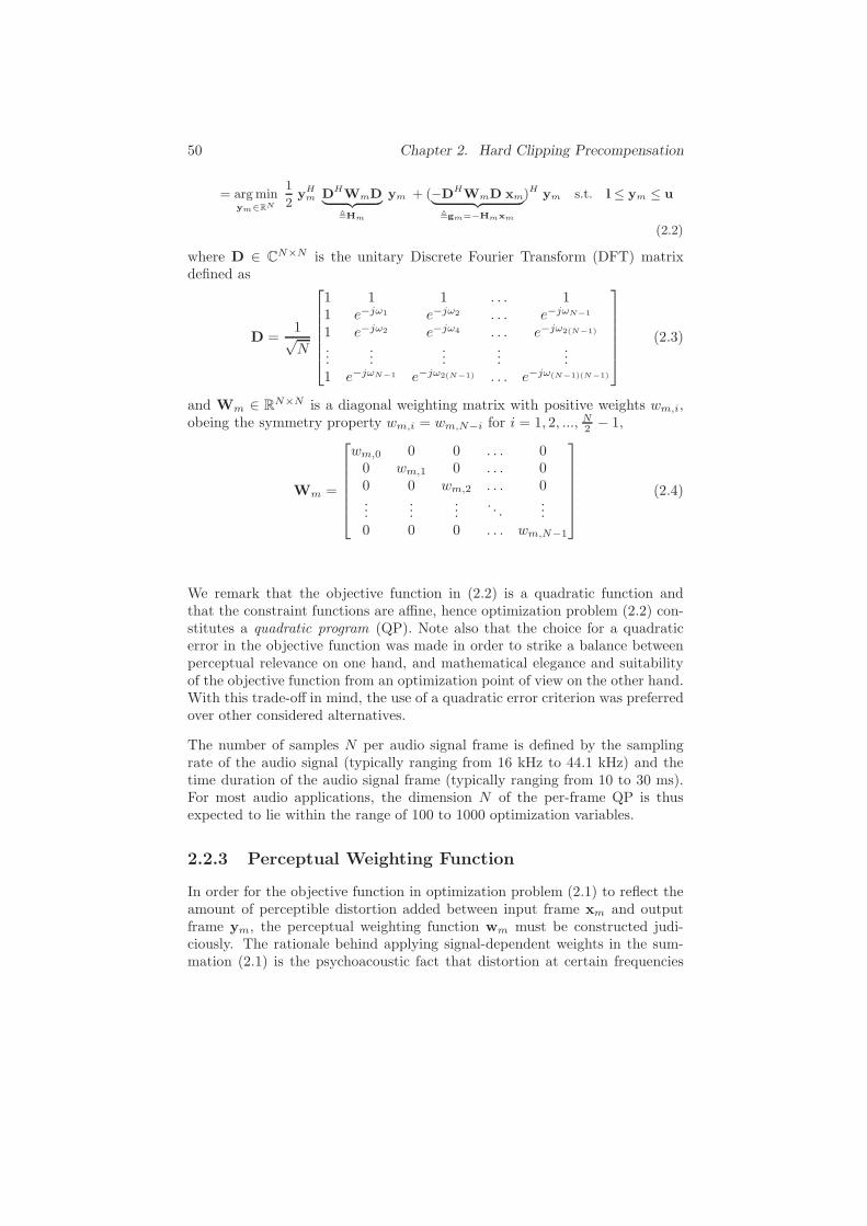
50 Chapter 2. Hard Clipping Precompensation
= argminym∈RN
1
2yHm D
HWmD
︸ ︷︷ ︸
,Hm
ym + (−DHWmD xm
︸ ︷︷ ︸
,gm=−Hmxm
)H ym s.t. l ≤ ym ≤ u
(2.2)
where D ∈ CN×N is the unitary Discrete Fourier Transform (DFT) matrix
defined as
D =1√N
1 1 1 . . . 11 e−jω1 e−jω2 . . . e−jωN−1
1 e−jω2 e−jω4 . . . e−jω2(N−1)
......
......
...1 e−jωN−1 e−jω2(N−1) . . . e−jω(N−1)(N−1)
(2.3)
and Wm ∈ RN×N is a diagonal weighting matrix with positive weights wm,i,obeing the symmetry property wm,i = wm,N−i for i = 1, 2, ..., N2 − 1,
Wm =
wm,0 0 0 . . . 00 wm,1 0 . . . 00 0 wm,2 . . . 0...
......
. . ....
0 0 0 . . . wm,N−1
(2.4)
We remark that the objective function in (2.2) is a quadratic function andthat the constraint functions are affine, hence optimization problem (2.2) con-stitutes a quadratic program (QP). Note also that the choice for a quadraticerror in the objective function was made in order to strike a balance betweenperceptual relevance on one hand, and mathematical elegance and suitabilityof the objective function from an optimization point of view on the other hand.With this trade-off in mind, the use of a quadratic error criterion was preferredover other considered alternatives.
The number of samples N per audio signal frame is defined by the samplingrate of the audio signal (typically ranging from 16 kHz to 44.1 kHz) and thetime duration of the audio signal frame (typically ranging from 10 to 30 ms).For most audio applications, the dimension N of the per-frame QP is thusexpected to lie within the range of 100 to 1000 optimization variables.
2.2.3 Perceptual Weighting Function
In order for the objective function in optimization problem (2.1) to reflect theamount of perceptible distortion added between input frame xm and outputframe ym, the perceptual weighting function wm must be constructed judi-ciously. The rationale behind applying signal-dependent weights in the sum-mation (2.1) is the psychoacoustic fact that distortion at certain frequencies
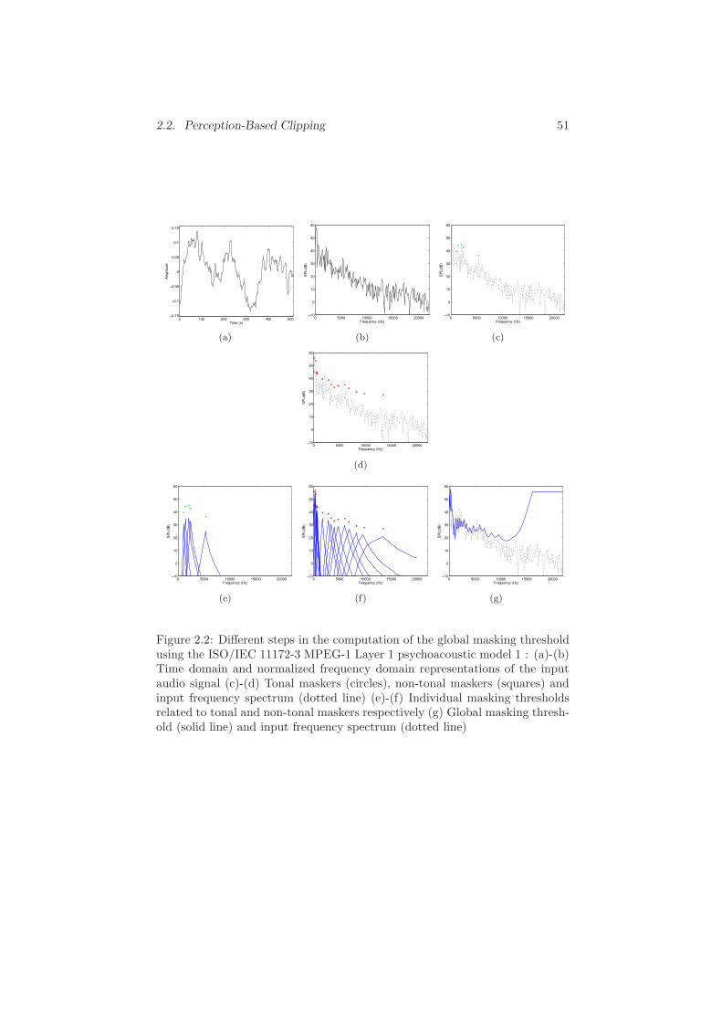
2.2. Perception-Based Clipping 51
0 100 200 300 400 500−0.15
−0.1
−0.05
0
0.05
0.1
0.15
Time (n)
Am
plit
ud
e
(a)
0 5000 10000 15000 20000−10
0
10
20
30
40
50
60
Frequency (Hz)
SP
L(d
B)
(b)
0 5000 10000 15000 20000−10
0
10
20
30
40
50
60
Frequency (Hz)
SP
L(d
B)
(c)
0 5000 10000 15000 20000−10
0
10
20
30
40
50
60
Frequency (Hz)
SP
L(d
B)
(d)
0 5000 10000 15000 20000−10
0
10
20
30
40
50
60
Frequency (Hz)
SP
L(d
B)
(e)
0 5000 10000 15000 20000−10
0
10
20
30
40
50
60
Frequency (Hz)
SP
L(d
B)
(f)
0 5000 10000 15000 20000−10
0
10
20
30
40
50
60
Frequency (Hz)
SP
L(d
B)
(g)
Figure 2.2: Different steps in the computation of the global masking thresholdusing the ISO/IEC 11172-3 MPEG-1 Layer 1 psychoacoustic model 1 : (a)-(b)Time domain and normalized frequency domain representations of the inputaudio signal (c)-(d) Tonal maskers (circles), non-tonal maskers (squares) andinput frequency spectrum (dotted line) (e)-(f) Individual masking thresholdsrelated to tonal and non-tonal maskers respectively (g) Global masking thresh-old (solid line) and input frequency spectrum (dotted line)

52 Chapter 2. Hard Clipping Precompensation
is more perceptible than distortion at other frequencies, and that the relativeperceptibility is mostly signal-dependent. Two phenomena of human auditoryperception are responsible for this,
• The absolute threshold of hearing is defined as the required intensity (dB)of a pure tone such that an average listener will just hear the tone in anoiseless environment. The absolute threshold of hearing is a function ofthe tone frequency and has been measured experimentally [15].
• Simultaneous masking is a phenomenon where the presence of certainspectral energy (the masker) masks the simultaneous presence of weakerspectral energy (the maskee), or in other words, renders it imperceptible.
Combining both phenomena, the instantaneous global masking threshold of asignal gives the amount of distortion energy (dB) at each frequency bin thatcan be masked by the signal. In this framework, we consider the input framexm to act as the masker, and ym − xm as the maskee. In other words, wemake the assumption that when the ear is presented with the output frameym, it is in fact presented with the input frame xm and the distortion ym−xm
simultaneously, and that the simultaneous masker-maskee relationship betweenboth signals can be exploited. By selecting the weights wm,i in (2.1) to beexponentially decreasing with the value of the global masking threshold of xm
at frequency bin i, the objective function effectively reflects the amount ofperceptible distortion introduced5. This can be specified as
wm,i =
10−αtm,i if 0 ≤ i ≤ N
2
10−αtm,N−i if N2 < i ≤ N − 1
(2.5)
where tm is the global masking threshold of xm (in dB). Appropriate values ofthe compression parameter α have been determined to lie in the range 0.04-0.06.
The instantaneous global masking threshold tm of an input frame xm is cal-culated using part of the ISO/IEC 11172-3 MPEG-1 Layer 1 psychoacousticmodel 1. A complete description of the operation of this psychoacoustic modelis out of the scope of this paper (we refer the reader to [9] and [14]). We willoutline the relevant steps in the computation of the instantaneous global mask-ing threshold and illustrate the result of each step on an example audio frame(see Figure 2.2):
1. Spectral analysis and SPL normalization: In this step a high-resolutionspectral estimate of the input frame is calculated, with spectral com-ponents expressed in terms of sound pressure level (SPL). After a nor-malization operation and a Hann window operation on the input signalframe, the PSD estimate is obtained through a 512-point Fast FourierTransform (FFT). Figure 2.2(a) shows the time-domain input signal,Figure 2.2(b) shows the resulting spectral estimate.
5Indeed, the terms in the summation of objective function (2.1) can then be seen toresemble to distortion-to-masker power ratios.
2.3. Optimization Methods 53
2. Identification of tonal and non-tonal maskers : It is known from psy-choacoustic research that the tonality of a masking component has aninfluence on its masking properties [16]. For this reason it is importantto discriminate between tonal maskers (defined as local maxima of thesignal spectrum) and non-tonal maskers. The output of the FFT is usedto determine the relevant tonal and non-tonal maskers in the spectrumof the audio signal. In a first phase, tonal maskers are identified atlocal maxima of the PSD: energy from three adjacent spectral compo-nents centered at the local maximum is combined to form a single tonalmasker. In a second phase, a single non-tonal masker per critical bandis formed by addition of all the energy from the spectral componentswithin the critical band that have not contributed to a tonal masker.
3. Decimation of maskers : In this step, the number of maskers is reducedusing two criteria. First, any tonal or non-tonal masker below the ab-solute threshold of hearing is discarded. Next, any pair of maskers oc-curring within a distance of 0.5 Bark is replaced by the stronger of thetwo. Figures 2.2(c) and 2.2(d) respectively depict the identified tonaland non-tonal maskers, after decimation.
4. Calculation of individual masking thresholds : an individual maskingthreshold is calculated for each masker in the decimated set of tonaland non-tonal maskers, using fixed psychoacoustic rules. Essentially,the individual masking threshold depends on the frequency, loudnesslevel and tonality of the masker. Figure 2.2(e) and 2.2(f) show the indi-vidual masking thresholds associated with tonal and non-tonal maskers,respectively.
5. Calculation of global masking threshold : Finally, the global maskingthreshold is calculated by a power-additive combination of the tonal andnon-tonal individual masking thresholds, and the absolute threshold ofhearing. This is illustrated in Figure 2.2(g).
2.3 Optimization Methods
The core of the perception-based clipping algorithm described in Section 2.2 isformed by the solution of an instance of optimization problem (2.2) for everyframe xm. Looking at the relatively high sampling rates (e.g. 44.1 kHz for CD-quality audio) and associated frame rates under consideration, it is clear thatreal-time operation of the algorithm calls for application-tailored optimizationmethods to solve the optimization problems in a fast and reliable way. Inthis section, we will discuss three different structure-exploiting optimizationmethods, whose common ground is the notion of convex optimization. Beforedoing so, we will first look at the properties of the optimization problem athand in this framework of convex optimization.

54 Chapter 2. Hard Clipping Precompensation
2.3.1 Convex Optimization Framework
Convex optimization is a subfield of mathematical optimization that studies aspecial class of mathematical optimization problems, namely convex optimiza-tion problems. This class can be formally defined as follows.
Definition 2.1 [Convex optimization problem] A convex optimization problemis one of the form
miny∈RN
f(y) s.t. hi(y) ≤ 0, i = 0, ...,K − 1 (2.6)
cTj y = dj , j = 0, ...,M − 1
in which the objective function f and the constraint functions h0, ..., hK−1 areconvex, which means they satisfy
f(ax+ by) ≤ af(x) + bf(y) (2.7)
hi(ax+ by) ≤ ahi(x) + bhi(y) (2.8)
for all x,y ∈ RN and all a, b ∈ R with a+ b = 1, a ≥ 0, b ≥ 0. 2
In particular, for quadratic programs, the next definition holds.
Definition 2.2 [Convex QP] A quadratic program (QP) is convex if and onlyif the Hessian matrix ∇2f(y) is positive semi-definite. It is strongly convex ifand only if ∇2f(y) is positive definite. 2
A fundamental property of convex optimization problems is that any localminimizer is a global minimizer. For strongly convex problems, it will also bethe unique minimizer.
We will now show that optimization problem (2.2) is a convex quadratic pro-gram, thereby looking a bit deeper into the structure of the Hessian matrixHm.
Definition 2.3 [Circulant matrix] A circulant matrix C is a square matrixhaving the form
C =
c0 cN−1 . . . c1
c1 c0 cN−1
...
c2 c1 c0. . .
c2 c1. . . cN−1
.... . .
cN−1 . . . c2 c1 c0
(2.9)

2.3. Optimization Methods 55
where each row is a cyclic shift of the row above it. 2
Theorem 2.4 (Diagonalization of circulant matrices [17, 18]) A circu-lant matrix C ∈ CN×N is diagonalized by the unitary DFT matrix D definedin (2.3), i.e.
C = DHΨD (2.10)
where Ψ = diag(ψ) contains the eigenvalues of C, which are obtained as theDFT of the first column of C,
ψl =N−1∑
k=0
cke−jωlk , l = 0, ..., N − 1 (2.11)
We can now state the following important properties of the Hessian matrixHm = DHWmD in (2.2):
Theorem 2.5 The Hessian matrix Hm = DHWmD ∈ RN×N in optimizationproblem (2.2) is real, symmetric, positive definite and circulant.
Proof : From (2.10) in Theorem 2.4, we readily see that Hm is circulant andWm contains its eigenvalues. By definitions (2.4)-(2.5), the elemens of Wm
are real and have even symmetry, so by (2.11) the first column of Hm will alsobe real and have even symmetry. From this we can see that Hm is real andsymmetric. As a symmetric matrix is positive definite if and only if all of itseigenvalues are positive, it remains to remark that the elements of Wm arepositive by construction (2.5) to conclude that Hm is positive definite. 2
Corollary 2.6 Optimization problem (2.2) is a strongly convex quadratic pro-gram.
Convex optimization problems can be solved reliably and efficiently by usingspecial methods for convex optimization. In particular, different iterative op-timization methods for solving (strongly) convex QPs have been presented.Essentially, three classes of methods can be distinguished. A first class arethe projected gradient methods, where only first-order information is used forsolving the optimization problem. These methods are conceptually simple andcomputationally cheap, but typically suffer from slow convergence, sometimespreventing their use in real-time applications. However, it is generally possibleto perform a convergence analysis and to establish useful polynomial com-putational complexity bounds for these algorithms [19]. A second class areinterior-point methods : these rely on heavier computational tasks, but have abetter convergence rate. Some interior-point methods are polynomial time, but
56 Chapter 2. Hard Clipping Precompensation
the complexity bounds are generally far off from practically observed ones [20].A third class are active set methods : these have a good perfomance in practice,but suffer from the drawback that in general no polynomial complexity boundscan be given [21].
In the remainder of this section, we will propose three different optimizationmethods tailored to QP (2.2), wherein the structure of the optimization prob-lem will be exploited.
• In subsection 2.3.2, an active set type of method will be proposed whichexploits the fact that only a small subset of the constraints will influencethe final solution.
• In subsections 2.3.3 and 2.3.4, two projected gradient methods will beproposed which exploit the circulant structure of the Hessian matrix andthe geometry of the convex feasible set.
2.3.2 Optimization Method 1: Dual Active Set Strategy
In [12], it was experimentally shown that general-purpose QP solvers are largelyinadequate to solve instances of QP (2.2) in real time. Therefore, an active setoptimization method was proposed that efficiently solves the dual optimizationproblem of (2.2).
Definition 2.7 [Dual optimization problem] For any primal optimization prob-lem of the form (2.6), the dual optimization problem is defined as the convexmaximization problem
maxλ∈RK ,ν∈RM
infy∈RN
[
f(y)−K−1∑
i=0
λihi(y)−M−1∑
j=0
νj(cTj y − dj)
︸ ︷︷ ︸
,L(y,λ,ν)
]
︸ ︷︷ ︸
,q(λ,ν)
s.t. λ ≥ 0
(2.12)where λ and ν are the vectors of Lagrange multipliers associated to the in-equality constraints and equality constraints respectively, L(y,λ,ν) is the La-grangian function and q(λ,ν) is the Lagrange dual function. 2
A primal optimization problem and its associated dual optimization problemare related in interesting ways. In general, the dual optimization problem canbe used to obtain a lower bound on the optimal value of the objective for theprimal problem. This primal-dual relationship is known as weak duality [22].
Theorem 2.8 (Weak duality) The optimal objective value p∗ of any primaloptimization problem (2.6) and the optimal objective value d∗ of the associated

2.3. Optimization Methods 57
dual optimization problem (2.12) are related as follows,
d∗ ≤ p∗ (2.13)
One of the main advantages of convex optimization problems is the fact thatthe dual optimization problem can be used directly for solving the primal op-timization problem. This primal-dual relationship is known as strong duality[22].
Theorem 2.9 (Strong duality) If the primal optimization problem (2.6) isconvex and it has a strictly feasible point, then primal optimization problem(2.6) and dual optimization problem (2.12) have the same optimal objectivevalue,
d∗ = p∗ (2.14)
Since in subsection 2.3.1 optimization problem (2.2) was shown to be a convexquadratic program, and zero is a strictly feasible point, it is clear from Theorem2.9 that it has a strong duality relationship with its dual counterpart. Weformulate this dual optimization problem as follows. First, the Lagrangianfunction L(ym,λm,u,λm,l) is given by
L(ym,λm,u,λm,l) = f(ym)− λTm,uhu(ym)− λ
Tm,lhl(ym)
=1
2(ym − xm)T Hm (ym − xm) + λ
Tm,u(ym − u) + λ
Tm,l(l− ym)
(2.15)
where λm,u,λm,l ∈ RN denote the vectors of Lagrange multipliers associatedto the upper clipping level constraints hu(ym) = [h0(ym) . . . hN−1(ym)]T andthe lower clipping level constraints hl(ym) = [hN (ym) . . . h2N−1(ym)]T , respec-tively. Then, the Lagrange dual function equals
q(λm,u,λm,l) = infym∈RN
L(ym,λm,u,λm,l)
= −1
2(λm,u − λm,l −Hmxm)TH−1
m (λm,u − λm,l −Hmxm)
− λTm,uu+ λT
m,ll+1
2xTmHmxm
(2.16)
Finally, the dual optimization problem can be formulated as
λ∗m = argmax
λm∈R2N
q(λm) s.t. λm ≥ 0
= argminλm∈R2N
1
2λTm ATH−1
m A︸ ︷︷ ︸
,Hm
λm + (BT1N −ATxm︸ ︷︷ ︸
,gm
)Tλm s.t. λm ≥ 0
(2.17)

58 Chapter 2. Hard Clipping Precompensation
where λm ∈ R2N , A ∈ R
N×2N and B ∈ RN×2N are defined as λm =
[λTm,u λT
m,l
]T, A =
[IN −IN
], and B =
[UIN −LIN
], with IN ∈
RN×N the identity matrix.
Computation of y∗m from λ∗
m is then straightforward,
y∗m = −H−1
m (Aλ∗m −Hmxm)
= xm −H−1m Aλ∗
m (2.18)
The dual optimization problem formulated in (2.17)-(2.18) can be solved ef-ficiently by exploiting the fact that only a small subset of the large number(2N) of inequality constraints are expected to influence the solution. Underthe assumption of a moderate clipping factor, indeed only a small number ofsamples in the input frame xm are expected to exceed the clipping levels. Aniterative external active set strategy is adopted, where the following steps areexecuted in each iteration (see Algorithm 1)6 :
1. Check which inequality constraints are violated in the previous solutioniterate. In case no inequality constraints are violated, the algorithmterminates.
2. Add the violated constraints to an active set S of constraints to bemonitored.
3. Solve a small-scale QP corresponding to (2.17) with those Lagrangemultipliers corresponding to constraints not in the active set S set tozero.
4. Compute the new solution iterate by evaluating (2.18).
Using this strategy of dualizing and iteratively adapting an appropriate sub-set of inequality constraints, a QP dimensionality reduction is achieved whichbrings along a significant computational complexity reduction. In effect, thesolution of QP (2.2) is found by solving a small number of small scale QPs(2.17) instead of by solving the full scale QP at once. From simulations, itis concluded that 4 external iterations generally suffice for solving an instanceof optimization problem (2.2). In comparison to general-purpose dense QPsolvers, the method achieves a reduction of computation time with a factorranging from 10 up to 200. Moreover, for clipping factors7 higher than 0.95,the method could potentially be used in a real-time clipping context [12].
Although computation times are reduced considerably, it has to be remarkedthat this optimization method still has a few shortcomings, possibly preventingit to be used reliably in real-time audio applications:
• First of all, the method’s computational complexity is seen to increase with
6We introduce in this algorithm the notation [·]km for the kth iterate of the mth frame7Clipping factor CF is defined as 1-(fraction of signal samples exceeding the upper or
lower clipping level)

2.3. Optimization Methods 59
Algorithm 1 Dual active set strategy
Input xm ∈ RN , Wm, L, UOutput y∗
m ∈ RN
1: y0m = xm
2: V0m = i|hi(y0
m) < 03: S0m = V0
m
4: k = 05: while Vk
m 6= ∅ do6: λk+1
m,i = 0, i /∈ Skm
7: Calculate λk+1m,i , i ∈ Skm as solution of small-scale QP defined in (2.17)
8: yk+1m = xm −H−1
m Aλk+1m [using (2.18)]
9: Collect index set of violated inequality constraints Vk+1m = i|hi(yk+1
m ) <0
10: Extend active set Sk+1m = Skm ∪ Vk+1
m
11: k = k + 112: end while13: y∗
m = ykm
increasing number of violated constraints in the input frame xm. That is, thecomputational complexity increases with decreasing clipping factors, makingit impossible to run the method in real time for low clipping factors.
• Secondly, it is practically impossible to derive certifying polynomial com-plexity bounds for the optimization method.
• Lastly, the iterative optimization method cannot be stopped early (i.e. beforeconvergence to the exact solution) to provide an approximate solution of theoptimization problem.
2.3.3 Optimization Method 2: Projected Gradient De-
scent
In this subsection, we present a projected gradient optimization method thatdeals with the different issues raised in subsection 2.3.2 concerning applicabil-ity in real time. First, a general description of the method is given. Then,the selection of an appropriate stepsize is discussed. Finally, the computationof approximate solutions is discussed and theoretical algorithmic complexitybounds are derived.
Description of the Method
Projected gradient methods are a class of iterative methods for solving opti-mization problems over convex sets. In each iteration, first a step is taken along
60 Chapter 2. Hard Clipping Precompensation
the negative gradient direction of the objective function, after which the resultis orthogonally projected onto the convex feasible set, thereby maintaining fea-sibility of the iterates [23]. A low computational complexity per iteration is themain asset of projected gradient methods, provided that the orthogonal pro-jection onto the convex feasible set and the gradient of the objective functioncan easily be computed.
For optimization problem (2.2), both these elements can indeed be computed atan extremely low computational complexity, by exploiting the structure of theHessian matrix and the convex feasible set. The main steps to be performedin the (k + 1)th iteration of the proposed projected gradient method are asfollows:
• Take a step with stepsize skm along the negative gradient direction:
yk+1m = yk
m − skm∇f(ykm) (2.19)
where using (2.2),
∇f(ykm) = Hm(yk
m − xm)
= DHWmD(ykm − xm). (2.20)
It is clear from (2.20) that the gradient computation can be performed at avery low computational complexity, by sequentially applying a DFT (multi-plication by D), an element-wise weighting (multiplication by Wm), and anIDFT (multiplication by DH) to the vector (yk
m−xm). An alternative inter-pretation is that we perform a matrix-vector multiplication of the circulantmatrix Hm with the vector (yk
m−xm). By exploiting the computational effi-ciency of the FFT algorithm, the gradient computation thus has a complexityof O(N log2N).
• Project yk+1m orthogonally onto the convex feasible set Q of (2.2), which is
defined asQ = ym ∈ R
N | l ≤ ym ≤ u (2.21)
The feasible set can be thought of as an N -dimensional box. An orthogonalprojection ΠQ(y
k+1m ) onto this N -dimensional box boils down to performing
a simple componentwise hard clipping operation (with lower bound L andupper bound U), i.e.
yk+1m = ΠQ(y
k+1m ) = argmin
z∈Q
1
2‖z− yk+1
m ‖22 (2.22)
where
yk+1m,i =
L if yk+1m,i < L
yk+1m,i if L ≤ yk+1
m,i ≤ U
U if yk+1m,i > U
, i = 0...N − 1 (2.23)
2.3. Optimization Methods 61
Stepsize Selection
Several rules for selecting stepsizes skm in projected gradient methods havebeen proposed in literature, e.g. fixed stepsizes, diminishing stepsizes, or linesearch rules [23]. Here a fixed stepsize is used, thereby avoiding the additionalcomputational complexity incurred by line searches. In [19], it is shown thatby choosing a fixed stepsize
skm =1
Cm
, ∀k ≥ 0 (2.24)
with Cm the Lipschitz constant of the gradient ∇f of (2.1) on the set Q (forframe m), a limit point of the sequence yk
m obtained by iteratively applying(2.19) and (2.23) is a stationary point. Because of the convexity of f , it is alocal minimum and hence a global minimum.
In order to establish the Lipschitz constant Cm of our problem, we introducethe next lemma.
Lemma 1 Let function f be twice continuously differentiable on set Q. Thegradient ∇f is Lipschitz continuous on set Q with Lipschitz constant C if andonly if
||∇2f(z)|| ≤ C , ∀z ∈ Q (2.25)
In other words, the Lipschitz constant of the gradient ∇f can be seen as anupper bound to the curvature of the objective function f . Using this lemma,we can easily show that the Lipschitz constant Cm is computed as
Cm = ||Hm||= max
1≤i≤Nβi(Hm)
= max1≤i≤N
βi(DHWmD)
= max0≤i≤N−1
wm,i (2.26)
where βi(Hm), i = 1...N , denote the eigenvalues of the Hessian matrix Hm.
Strong convexity assumes that in addition to an upper bound also a lowerbound on the curvature of the objective function can be found, determined bythe convexity parameter µm.
Lemma 2 Let function f be twice continuously differentiable on set Q. Thefunction f is strongly convex on set Q with convexity parameter µ if and onlyif there exists µ > 0 such that
∇2f(z) ≥ µI , ∀z ∈ Q
62 Chapter 2. Hard Clipping Precompensation
Algorithm 2 Projected gradient method
Input xm ∈ RN , y0m ∈ Q, Wm, L, U ,
Output y∗m ∈ R
N
1: k = 02: Calculate Lipschitz constant Cm [using (2.26)]3: while convergence is not reached do4: yk+1
m = ykm − 1
Cm∇f(yk
m) [using (2.20)]
5: yk+1m = ΠQ(y
k+1m ) [using (2.23)]
6: k = k + 17: end while8: y∗
m = ykm
Using the former lemma, we can prove that for our objective function theconvexity parameter µm can be computed as
µm = min1≤i≤N
βi(Hm)
= min1≤i≤N
βi(DHWmD)
= min0≤i≤N−1
wm,i (2.27)
The ratio κm = Cm
µmis called the condition number.
Algorithmic Complexity and Approximate Solutions
The proposed projected gradient optimization method is summarized in Al-gorithm 2. Clearly, the computational complexity of one iteration is seen tobe extremely low. Moreover, the shortcomings of the optimization method 1presented in subsection 2.3.2 are dealt with:
• It is possible to solve the optimization problem inexactly by stopping theiterative optimization method before convergence to the exact solution y∗
m
is reached. The iterates ykm of the proposed projected gradient method are
feasible by construction. Moreover, the sequence f(ykm) can be proved to
be monotonically decreasing. Hence, stopping the method after any numberof iterations η will result in a feasible point yη
m for which f(yηm) ≤ f(y0
m).We can then define the obtained solution accuracy as ǫ = f(yη
m)− f(y∗m).
• It is possible to derive polynomial upper and lower bounds on the algorith-mic complexity, i.e. the number of necessary iterations of the optimizationmethod as a function of the obtained solution accuracy ǫ, as we will shownext.

2.3. Optimization Methods 63
For the class of convex optimization problems with strongly convex objectivefunctions, a general lower bound on the algorithmic complexity was derivedthat holds for all iterative first-order methods [19, Ch. 2]:
Theorem 2.10 For any starting point y0m ∈ RN , for any first-order projected
gradient method, and for any closed convex set Q, there exists a strongly convex,continuously differentiable function f with Lipschitz constant Cm and convexityparameter µm = Cm
κm(where κm > 1), such that we have
f(ykm)− f(y∗
m) ≥ µm
2
(√κm − 1√κm + 1
)2k
||y0m − y∗
m||2, ∀k (2.28)
Also, for the same problem class, an upper bound on the algorithmic complexityof the projected gradient method used in Algorithm 2 was derived [19, Ch. 2]:
Theorem 2.11 Let f be a strongly convex, continuously differentiable functionwith Lipschitz constant Cm and convexity parameter µm = Cm
κm(where κm >
1), and let Q be a convex feasible set. Then the projected gradient methoddescribed in Algorithm 2 with fixed stepsize 1
Cmgenerates a sequence yk
mwhich converges as follows:
f(ykm)− f(y∗
m) ≤ µm
2
(κm − 1
κm + 1
)2k
||y0m − y∗
m||2, ∀k. (2.29)
As the general algorithmic complexity lower bound (2.28) for first-order opti-mization methods, and the specific algorithmic complexity upper bound (2.29)for the projected gradient optimization method described in Algorithm 2 differby an order of magnitude, it can be concluded that the proposed optimizationmethod is not optimal in terms of convergence.
2.3.4 Optimization Method 3: Optimal Projected Gradi-
ent Descent
From the complexity bounds given in subsection 2.3.3 it might be expectedthat it is theoretically possible for a first-order optimization method to havea better convergence rate than optimization method 2. Indeed, if there existsa first-order method for which the complexity upper bound is proportional tothe complexity lower bound for a given problem class, this method could becalled optimal for that problem class [19]. In this subsection, we present aprojected gradient optimization method that reaches an optimal convergencefor the class of convex optimization problems with strongly convex objectivefunctions. This method was first proposed in [19] and variants of the method

64 Chapter 2. Hard Clipping Precompensation
Algorithm 3 Optimal projected gradient method
Input xm ∈ RN , y0m = c0m ∈ Q, Wm, γ0m ∈ (0, 1), L, U
Output y∗m ∈ R
N
1: Calculate Lipschitz constant Cm [using (2.26)]2: Calculate convexity parameter µm [using (2.27)]3: κm = Cm
µm
4: k = 05: while convergence is not reached do6: yk+1
m = ckm − 1Cm
∇f(ckm)
7: yk+1m = ΠQ(y
k+1m ) [using (2.23)]
8: Calculate γk+1m from (γk+1
m )2 = (1− γk+1m )(γkm)2 + κmγ
k+1m
9: δkm =γkm(1−γk
m)
(γkm)2+γ
k+1m
10: ck+1m = yk+1
m + δkm(yk+1m − yk
m)11: k = k + 112: end while13: y∗
m = ykm
have been applied in diverse applications, e.g. for real-time model predictivecontrol [20].
Algorithm 3 summarizes the optimal projected gradient optimization method.We note the following differences compared to Algorithm 2:
• Knowledge of the convexity parameter µm is incorporated.• In each iteration, a standard projected gradient step is performed on a
potentially infeasible weighted sum of two previous feasible iterates.
It is again possible to derive polynomial an upper bound on the algorithmiccomplexity of the projected gradient method used in Algorithm 3, i.e. thenumber of necessary iterations of this optimization method as a function of thesolution accuracy ǫ [19, Ch. 2]:
Theorem 2.12 Let f be a strongly convex, continuously differentiable functionwith Lipschitz constant Cm and convexity parameter µm = Cm
κm(where κm > 1),
and let Q be a convex feasible set. Then the projected gradient method describedin Algorithm 3 generates a sequence yk
m which converges as follows:
f(ykm)− f(y∗
m) ≤ Cm min
(
1−√µm
Cm
)k
,4
(k + 2)2
||y0m − y∗
m||2. (2.30)
From (2.28), the minimum number of necessary iterations to find ykm satisfying

2.3. Optimization Methods 65
Table 2.1: Algorithmic and arithmetic complexity of optimization methods 2and 3Algorithm Algorithmic complexity Arithmetic complexity per iteration
Method 2 κm log 4CmNU2
ǫ519 N log2N − 61
18N
Method 3√κm log 4CmNU2
ǫ519 N log2N − 7
18N
f(ykm)− f(y∗
m) ≤ ǫ is
kminm =
√κm − 1
4
(
log1
ǫ+ log
µm
2+ 2 log ||y0
m − y∗m||
)
(2.31)
From (2.30), the maximum number of necessary iterations to find ykm satisfying
f(ykm)− f(y∗
m) ≤ ǫ is
kmaxm =
√κm
(
log1
ǫ+ logCm + 2 log ||y0
m − y∗m||
)
(2.32)
Hence, the main term in the upper bound estimate (2.32),√κm log 1
ǫ, is pro-
portional to the lower bound (2.31), proving this optimization method to bean optimal first-order method for the class of strongly convex optimizationproblems.
Table 2.1 summarizes the computational complexity results of optimizationmethods 2 and 3. For both methods, the algorithmic complexity as wellas the arithmetic complexity per iteration (in terms of number of real addi-tions and multiplications) is given. The algorithmic complexity results arestraightforwardly found from upper bounds (2.29) and (2.30) by incorporat-ing ||y0
m − y∗m|| = 2
√NU as the (worst-case) maximum distance between
two points in the feasible set Q defined in (2.21)8, where it is assumed thatU = −L. In the arithmetic complexity computations, estimates were usedfor the arithmetic complexity of a FFT with power-of-two length N , as de-rived in [24]: namely, 17
9 N log2N − 8927N + O(log2N) for a real-data FFT,
and 349 N log2N − 124
27 N + O(log2N) for a complex-data FFT. In conclusion,optimization method 3 has a significantly better algorithmic complexity com-pared to optimization method 2, and this for a negligibly higher arithmeticcomplexity per iteration.
8The length of an N-agonal in an N-dimensional hypercube with side length 2U equals2√NU .

66 Chapter 2. Hard Clipping Precompensation
2.4 Simulation Results
2.4.1 Comparative Evaluation of Perceived Audio Qual-
ity
For audio quality evaluation purposes, a test database consisting of 24 audioexcerpts was compiled (16 bit mono, 44.1 kHz). The excerpts were selected so asto cover different music styles, melodic and rythmic textures, instrumentationsand dynamics, as well as different speech types (see Table 2.2 for details). Afirst set of excerpts (numbers 1-11) was extracted from different commercialaudio CDs. A second set of excerpts (numbers 12-16) was extracted froman ITU CD-ROM associated to Recommendation BS.1387-1, which contains adatabase (DB3) used for validating the conformance of implementations to thisrecommendation [25]. A third set of excerpts (numbers 17-20) was extractedfrom the HINT speech database [26]. A fourth set of excerpts (numbers 21-24)was extracted from the VoxForge speech corpus [27].
Each audio signal in the test database was processed by three different clippingalgorithms:
• Hard symmetrical clipping, where the input-output characteristic is de-fined as
y[n] =
x[n], |x[n]| ≤ Usgn(x[n])U, |x[n]| > U
(2.33)
• Soft symmetrical clipping [3], where the input-output characteristic isdefined as a linearized hyperbolic tangent function which is linear forinputs below a parametric amplitude level r,
y[n] =
x[n], |x[n]| ≤ r
sgn(x[n])[
(U − r) tanh(
|x[n]|−r
U−r
)
+ r]
, |x[n]| > r(2.34)
here used with parameter setting r = 0.8U .• Perception-based clipping as described in this paper, with parameter val-
ues N = 512, P = 128, α = 0.04, and application of optimization method3 with a solution accuracy of ǫ = 10−12 for all instances of (2.2).
This processing was performed for eight clipping factors 0.70, 0.80, 0.85, 0.90,0.95, 0.97, 0.98, 0.999. For each of a resulting total of 24×8×3=576 processedaudio signals, two objective measures of perceived audio quality were calcu-lated, which aim to predict the subjective audio quality score that would beattributed to the processed audio signal by an average human listener. Taking
9Note that the clipping factor above which a normal-hearing listener does not perceivehard clipping distortion has been subjectively evaluated to be higher than 0.99 for speech[39], and 0.997 for music [40].
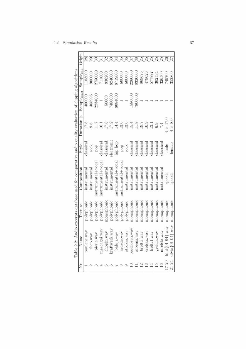
2.4. Simulation Results 67
Table
2.2:Audio
excerpts
database
usedforcomparativeaudio
quality
evaluationofclippingalgorithms
Nr.
Name
Texture
Composition
Style
Duration[s]
Sample
start
Sample
end
Origin
1poulenc.wav
polyphonic
instrumental
classical
17.8
400000
1183000
[28]
2rhcp.wav
polyphonic
instrumental
rock
9.8
468996
900000
[29]
3pierle.wav
polyphonic
instrumental+
vocal
pop
11.7
2234000
2750000
[30]
4mascagni.wav
polyphonic
instrumental+
vocal
classical
16.1
1711000
[31]
5chopin.wav
monophonic
instrumental
classical
17.8
50000
836200
[32]
6kraftwerk.wav
polyphonic
instrumental
electronic
17.2
7480000
8240000
[33]
7baloji.wav
polyphonic
instrumental+
vocal
hip
hop
14.4
8084000
8719000
[34]
8arcade.wav
polyphonic
instrumental+
vocal
pop
13.6
1600000
[35]
9strokes.wav
polyphonic
instrumental
rock
13.6
1600000
[36]
10
beethoven.wav
monophonic
instrumental
classical
15.4
1580000
2260000
[37]
11
albeniz.wav
monophonic
instrumental
classical
11.8
7800000
8320000
[38]
12
breftri.wav
monophonic
instrumental
classical
19.7
1869675
[25]
13
crefsax.wav
monophonic
instrumental
classical
10.9
1479026
[25]
14
freftr1.wav
monophonic
instrumental
classical
13.1
1577887
[25]
15
grefcla.wav
monophonic
instrumental
classical
6.9
1302534
[25]
16
mrefcla.wav
monophonic
instrumental
classical
7.4
1326500
[25]
17-20
hint01-04.wav
monophonic
speech
male
4×
17.0
1749700
[26]
21-24
silvia0
1-04.wav
monophonic
speech
female
4×
8.0
1352800
[27]

68 Chapter 2. Hard Clipping Precompensation
(a) (b)
Figure 2.3: Block diagrams of the used objective measures of perceived audioquality : (a) PEAQ Basic version (adapted from [25]) (b) Rnonlin
a reference signal (i.e. the clean signal) and a signal under test (i.e. the pro-cessed signal) as an input, such an objective measure of perceived audio qualityis calculated through sequential application of a psychoacoustic model and acognitive model, and resultingly attributes a perceived audio quality score tothe signal under test with respect to the reference signal (see Figure 2.3).
A first objective measure of perceived audio quality was calculated using theBasic Version of the PEAQ (Perceptual Evaluation of Audio Quality) recom-mendation [25]. A block diagram representation of this method is shown inFigure 2.3(a). The resulting Objective Difference Grade (ODG) predicts thebasic audio quality of the signal under test with respect to the reference signal,and has a range between 0 and - 4, corresponding to the ITU-R five gradeimpairment scale depicted in Figure 2.4.
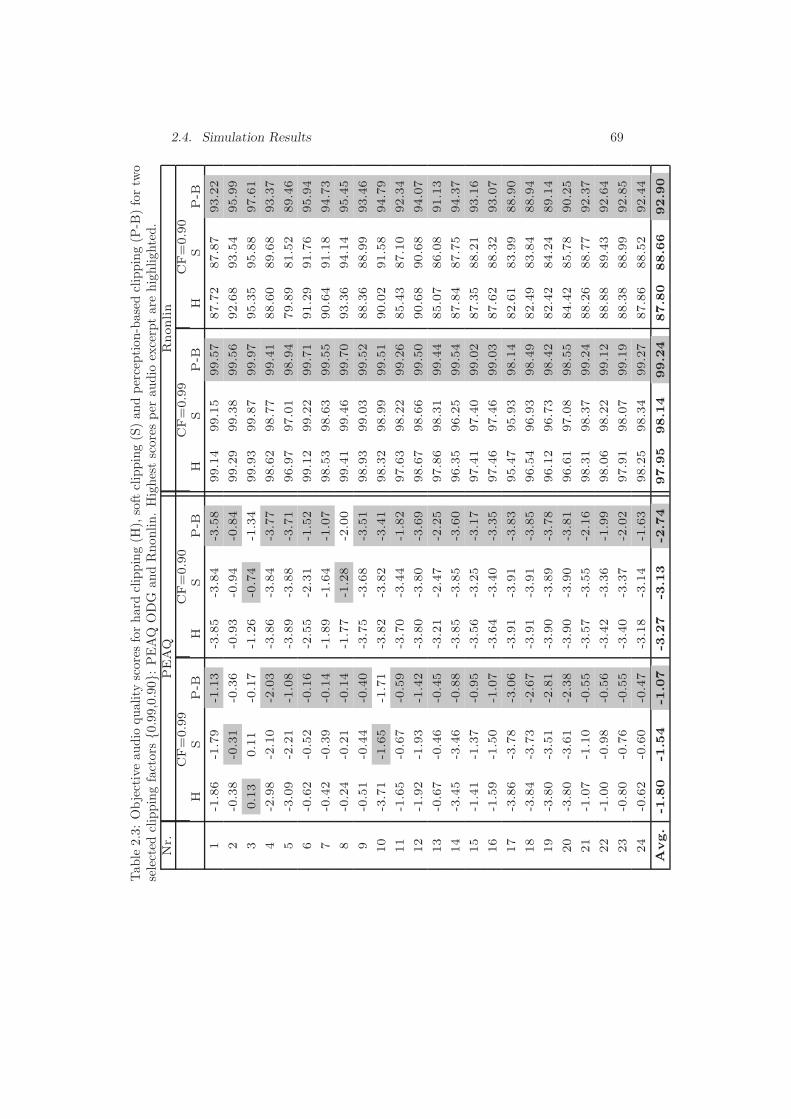
2.4. Simulation Results 69Table
2.3:Objectiveaudio
quality
scoresforhard
clipping(H
),softclipping(S)andperception-basedclipping(P
-B)fortw
oselected
clippingfactors
0.99,0.90:
PEAQ
ODG
andRnonlin.Highestscoresper
audio
excerptare
highlighted.
Nr.
PEAQ
Rnonlin
CF=0.99
CF=0.90
CF=0.99
CF=0.90
HS
P-B
HS
P-B
HS
P-B
HS
P-B
1-1.86
-1.79
-1.13
-3.85
-3.84
-3.58
99.14
99.15
99.57
87.72
87.87
93.22
2-0.38
-0.31
-0.36
-0.93
-0.94
-0.84
99.29
99.38
99.56
92.68
93.54
95.99
30.13
0.11
-0.17
-1.26
-0.74
-1.34
99.93
99.87
99.97
95.35
95.88
97.61
4-2.98
-2.10
-2.03
-3.86
-3.84
-3.77
98.62
98.77
99.41
88.60
89.68
93.37
5-3.09
-2.21
-1.08
-3.89
-3.88
-3.71
96.97
97.01
98.94
79.89
81.52
89.46
6-0.62
-0.52
-0.16
-2.55
-2.31
-1.52
99.12
99.22
99.71
91.29
91.76
95.94
7-0.42
-0.39
-0.14
-1.89
-1.64
-1.07
98.53
98.63
99.55
90.64
91.18
94.73
8-0.24
-0.21
-0.14
-1.77
-1.28
-2.00
99.41
99.46
99.70
93.36
94.14
95.45
9-0.51
-0.44
-0.40
-3.75
-3.68
-3.51
98.93
99.03
99.52
88.36
88.99
93.46
10
-3.71
-1.65
-1.71
-3.82
-3.82
-3.41
98.32
98.99
99.51
90.02
91.58
94.79
11
-1.65
-0.67
-0.59
-3.70
-3.44
-1.82
97.63
98.22
99.26
85.43
87.10
92.34
12
-1.92
-1.93
-1.42
-3.80
-3.80
-3.69
98.67
98.66
99.50
90.68
90.68
94.07
13
-0.67
-0.46
-0.45
-3.21
-2.47
-2.25
97.86
98.31
99.44
85.07
86.08
91.13
14
-3.45
-3.46
-0.88
-3.85
-3.85
-3.60
96.35
96.25
99.54
87.84
87.75
94.37
15
-1.41
-1.37
-0.95
-3.56
-3.25
-3.17
97.41
97.40
99.02
87.35
88.21
93.16
16
-1.59
-1.50
-1.07
-3.64
-3.40
-3.35
97.46
97.46
99.03
87.62
88.32
93.07
17
-3.86
-3.78
-3.06
-3.91
-3.91
-3.83
95.47
95.93
98.14
82.61
83.99
88.90
18
-3.84
-3.73
-2.67
-3.91
-3.91
-3.85
96.54
96.93
98.49
82.49
83.84
88.94
19
-3.80
-3.51
-2.81
-3.90
-3.89
-3.78
96.12
96.73
98.42
82.42
84.24
89.14
20
-3.80
-3.61
-2.38
-3.90
-3.90
-3.81
96.61
97.08
98.55
84.42
85.78
90.25
21
-1.07
-1.10
-0.55
-3.57
-3.55
-2.16
98.31
98.37
99.24
88.26
88.77
92.37
22
-1.00
-0.98
-0.56
-3.42
-3.36
-1.99
98.06
98.22
99.12
88.88
89.43
92.64
23
-0.80
-0.76
-0.55
-3.40
-3.37
-2.02
97.91
98.07
99.19
88.38
88.99
92.85
24
-0.62
-0.60
-0.47
-3.18
-3.14
-1.63
98.25
98.34
99.27
87.86
88.52
92.44
Avg.
-1.8
0-1
.54
-1.0
7-3
.27
-3.1
3-2
.74
97.9
598.1
499.2
487.8
088.6
692.9
0
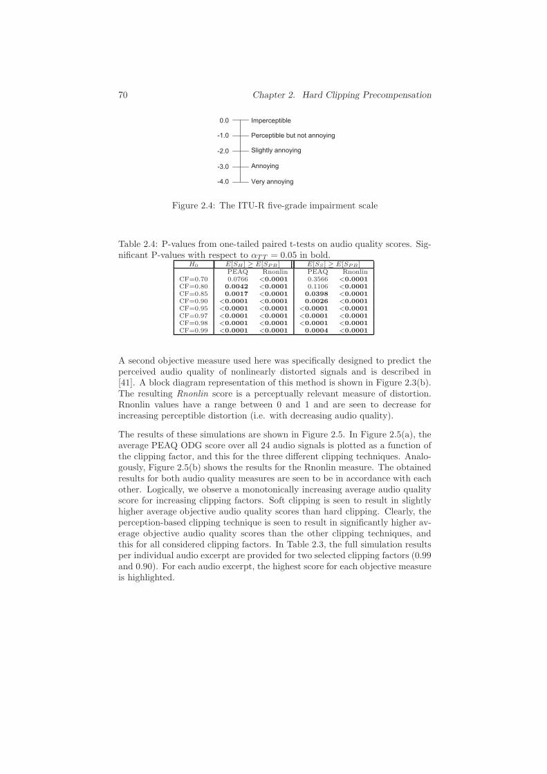
70 Chapter 2. Hard Clipping Precompensation
0.0
-1.0
-2.0
-3.0
-4.0
Imperceptible
Perceptible but not annoying
Slightly annoying
Annoying
Very annoying
Figure 2.4: The ITU-R five-grade impairment scale
Table 2.4: P-values from one-tailed paired t-tests on audio quality scores. Sig-nificant P-values with respect to αTT = 0.05 in bold.
H0 E[SH ] ≥ E[SPB ] E[SS ] ≥ E[SPB ]PEAQ Rnonlin PEAQ Rnonlin
CF=0.70 0.0766 <0.0001 0.3566 <0.0001
CF=0.80 0.0042 <0.0001 0.1106 <0.0001
CF=0.85 0.0017 <0.0001 0.0398 <0.0001
CF=0.90 <0.0001 <0.0001 0.0026 <0.0001
CF=0.95 <0.0001 <0.0001 <0.0001 <0.0001
CF=0.97 <0.0001 <0.0001 <0.0001 <0.0001
CF=0.98 <0.0001 <0.0001 <0.0001 <0.0001
CF=0.99 <0.0001 <0.0001 0.0004 <0.0001
A second objective measure used here was specifically designed to predict theperceived audio quality of nonlinearly distorted signals and is described in[41]. A block diagram representation of this method is shown in Figure 2.3(b).The resulting Rnonlin score is a perceptually relevant measure of distortion.Rnonlin values have a range between 0 and 1 and are seen to decrease forincreasing perceptible distortion (i.e. with decreasing audio quality).
The results of these simulations are shown in Figure 2.5. In Figure 2.5(a), theaverage PEAQ ODG score over all 24 audio signals is plotted as a function ofthe clipping factor, and this for the three different clipping techniques. Analo-gously, Figure 2.5(b) shows the results for the Rnonlin measure. The obtainedresults for both audio quality measures are seen to be in accordance with eachother. Logically, we observe a monotonically increasing average audio qualityscore for increasing clipping factors. Soft clipping is seen to result in slightlyhigher average objective audio quality scores than hard clipping. Clearly, theperception-based clipping technique is seen to result in significantly higher av-erage objective audio quality scores than the other clipping techniques, andthis for all considered clipping factors. In Table 2.3, the full simulation resultsper individual audio excerpt are provided for two selected clipping factors (0.99and 0.90). For each audio excerpt, the highest score for each objective measureis highlighted.

2.4. Simulation Results 71
0.7 0.75 0.8 0.85 0.9 0.95 1−4
−3.5
−3
−2.5
−2
−1.5
−1
−0.5
0
Clipping factor
Me
an
PE
AQ
ob
jective
diffe
ren
ce
gra
de
Hard clipping
Soft clipping
Perception−based clipping
(a) PEAQ Basic Version
0.7 0.75 0.8 0.85 0.9 0.95 10.7
0.75
0.8
0.85
0.9
0.95
1
Clipping factor
Me
an
Rn
on
lin s
co
re
Hard clipping
Soft clipping
Perception−based clipping
(b) Rnonlin
Figure 2.5: Comparative evaluation of different clipping techniques in terms ofobjective perceived audio quality: (a) mean PEAQ ODG and (b) mean Rnonlinscores for signals processed by hard clipping, soft clipping and perception-basedclipping as a function of the clipping factor

72 Chapter 2. Hard Clipping Precompensation
In order to infer statistically significant conclusions on the comparative audioquality performance of the three clipping algorithms under study, a statisti-cal analysis was performed on the obtained set of PEAQ ODG and Rnonlinscores. Let us represent the audio quality scores resulting from hard clipping,soft-clipping and perception-based clipping for a given clipping factor by ran-dom variables SH , SS , and SPB , respectively. Under the assumption thatthese random variables follow a normal probability distribution10, we testedthe two following statistical hypotheses based on the sample data. The firstnull hypothesis H0 and its alternative H1 are formulated as follows,
H0 : E[SH ] ≥ E[SPB ] (2.35)
H1 : E[SPB ] > E[SH ] (2.36)
The second null hypothesis H0 and its alternative H1 are formulated as follows,
H0 : E[SS ] ≥ E[SPB] (2.37)
H1 : E[SPB] > E[SS ] (2.38)
These two statistical hypotheses were tested for all considered clipping factors,and for both audio quality measures. All statistical hypotheses were testedusing one-tailed paired t-tests with significance level αTT = 0.05. The resultingone-sided P-values are synthesized in Table 2.4. For PEAQ scores, the firstnull hypothesis (2.35) can be rejected in favor of the alternative (2.36) forclipping factors of 0.80 and higher. The second null hypothesis (2.37) canbe rejected in favor of the alternative (2.38) for clipping factors of 0.85 andhigher. For Rnonlin scores, both null hypotheses can be rejected in favor of thealternative for all considered clipping factors. We can conclude that there isstrong statistical evidence that the perception-based clipping technique will ingeneral deliver signals with a higher perceptual audio quality compared to theother considered clipping techniques, and this for moderate to high clippingfactors.
2.4.2 Experimental Evaluation of Algorithmic Complex-
ity
In order to assess experimentally the validity of the theoretical algorithmiccomplexity bounds of the projected gradient optimization methods 2 and 3described in subsections 2.3.3 and 2.3.4, a simulation was conducted as follows.For optimization methods 2 and 3, the number of iterations needed to reachsolution accuracies ǫ = 10−4, 10−5,...,10−10 was determined for a subset ofthe instances of optimization problem (2.2) occurring in our test database of24 audio signals. This was performed for six clipping factors 0.85, 0.90, 0.95,0.97, 0.98, 0.99.
10The validity of this assumption was verified for our sample data using the Jarque-Beranormality test [42] at significance level αJB = 0.05.

2.4. Simulation Results 73
10e−4 10e−5 10e−6 10e−7 10e−8 10e−9 10e−100
250
500
750
1000
1250
1500
Solution accuracy ε
Num
ber
of
itera
tions
121314151617181920212223242526272829303132333435363738394041424344454647484950515253
Method 2
Method 3
10e−4 10e−1010e−6 10e−7 10e−8 10e−910e−5 10e−610e−510e−4 10e−7 10e−8 10e−9 10e−10
Figure 2.6: Boxplot of number of iterations vs solution accuracy for optimiza-tion methods 2 and 3
In Figure 2.6, the simulation results per optimization method are summarizedin the form of a boxplot for each solution accuracy, depicting graphically theminimum, lower quartile, median, upper quartile and maximum values of thenumber of iterations. The dotted lines connect the median number of iterationsof both optimization methods for different solution accuracies. We observe thatthe median (the same holds for the maximum) number of iterations follows adifferent curve depending on the optimization method: optimization method3 is seen to have a significantly better algorithmic complexity compared tooptimization method 2, as was derived theoretically in subsections 2.3.3 and2.3.4.
2.4.3 Applicability in Real-Time Context: Effect of Solu-
tion Accuracy ǫ on Perceived Audio Quality
In a real-time processing context, the number of clock cycles that can be spenton solving an instance of optimization problem (2.2) is strictly limited. Inview of this, several computationally efficient convex optimization methodstailored to the optimization problem were presented in Section 2.3. It wasshown that the iterative projected gradient optimization methods 2 and 3 havethe advantage that approximate solutions can be computed, which makes itpossible to adhere to the imposed real-time deadlines. The question remains asto how approximately solving the optimization problems affects the perceivedaudio quality of the resulting output signal. In order to assess this effect,
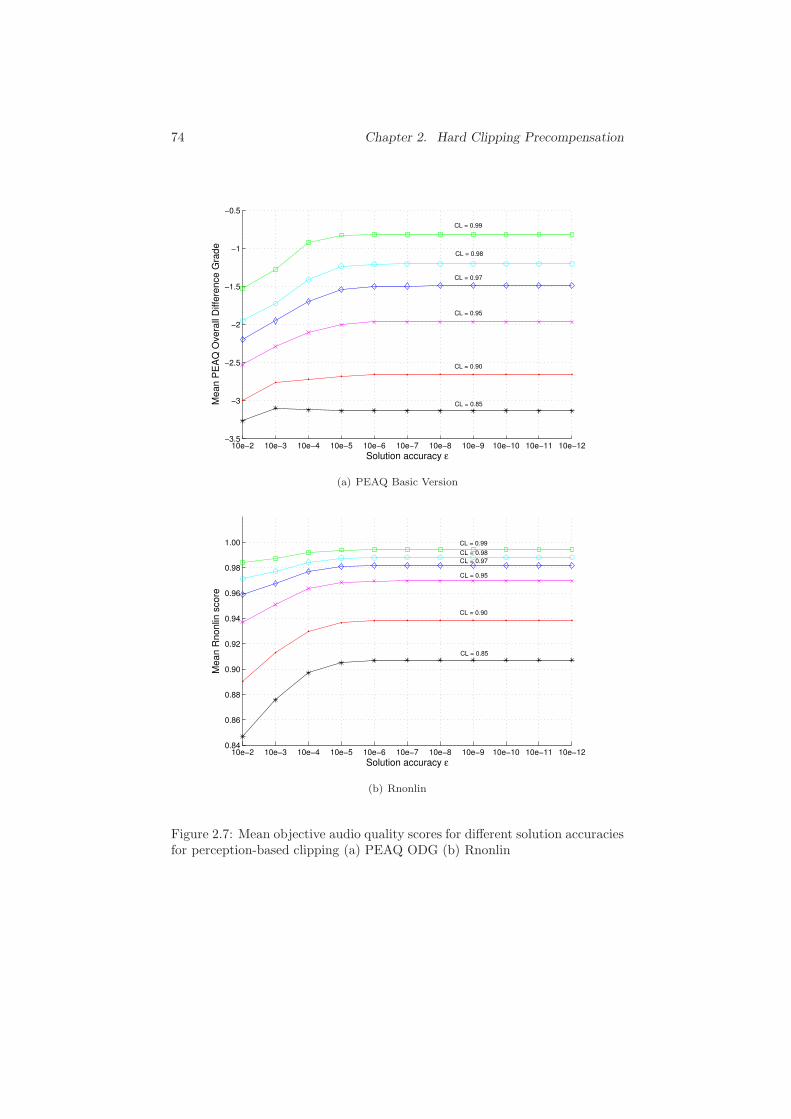
74 Chapter 2. Hard Clipping Precompensation
10e−2 10e−3 10e−4 10e−5 10e−6 10e−7 10e−8 10e−9 10e−10 10e−11 10e−12−3.5
−3
−2.5
−2
−1.5
−1
−0.5
Solution accuracy ε
Me
an
PE
AQ
Ove
rall
Diffe
ren
ce
Gra
de
CL = 0.99
CL = 0.98
CL = 0.97
CL = 0.95
CL = 0.90
CL = 0.85
(a) PEAQ Basic Version
10e−2 10e−3 10e−4 10e−5 10e−6 10e−7 10e−8 10e−9 10e−10 10e−11 10e−120.84
0.86
0.88
0.90
0.92
0.94
0.96
0.98
1.00
Solution accuracy ε
Me
an
Rn
on
lin s
co
re
CL = 0.90
CL = 0.85
CL = 0.99
CL = 0.98
CL = 0.97
CL = 0.95
(b) Rnonlin
Figure 2.7: Mean objective audio quality scores for different solution accuraciesfor perception-based clipping (a) PEAQ ODG (b) Rnonlin

2.5. Conclusions 75
PEAQ ODG and Rnonlin scores were calculated for a subset of the signals inour test database, each of which was processed by perception-based clippingfor optimization problem solution accuracies ǫ = 10−2, 10−3,...,10−12. Thiswas performed for six clipping factors 0.85, 0.90, 0.95, 0.97, 0.98, 0.99.
In Figures 2.7(a) and 2.7(b), the resulting mean PEAQ ODG and Rnonlinscores over all audio signals are plotted as a function of the solution accuracy,and this for all considered clipping factors. We observe that, according toboth measures, the mean audio quality is affected negatively for low solutionaccuracies, increases nearly monotonically with increasing solution accuracies,and saturates at a solution accuracy that depends on the clipping factor. Ir-respective of the clipping factor, we observe that no further improvement inmean audio quality scores is obtained for higher solution accuracies than 10−6.Hence, ǫ = 10−6 can be put forward as an experimentally established sufficientsolution accuracy for all considered clipping factors, such that no sacrifice interms of audio quality is made.
For parameter values N = 512, P = 128 and sampling rate of 44.1 kHz,the real-time computation time limit for solving one instance of optimizationproblem (2.2) is equal to 8.7 ms. In our simulation setting11, this correspondsto an iteration limit of roughly 200 iterations for optimization methods 2 or3 (neglecting here the small difference in arithmetic complexity per iterationbetween both methods as shown in Table 2.1). Looking back at Figure 2.6, wesee that even for the worst-case instances in our test database, optimizationmethod 3 meets the real-time iteration limit for solution accuracies up to 10−10,which largely surpasses the required solution accuracy of 10−6.
2.5 Conclusions
In this paper, we have presented a novel algorithm for real-time perception-based clipping of audio signals. By including a psychoacoustic model andembedding convex optimization into the algorithm, it is possible to explic-itly minimize the perceptible distortion introduced by clipping. From com-parative audio quality evaluation experiments, it has been concluded that theperception-based clipping algorithm results in significantly higher objective au-dio quality scores than standard clipping techniques, and this for moderate tohigh clipping factors. Furthermore, three optimization methods aimed at effi-ciently solving the convex optimization problems were derived. The reliable useof optimization method 3 in real-time applications was seen to be supported bytheoretically derived complexity bounds as well as by simulation experiments.
In a broader view, the results presented in this paper suggest that embedded
11All simulations were performed on a GenuineIntel CPU @2826 Mhz

76 Bibliography
convex optimization is a very promising paradigm in real-time audio processingapplications, with numerous potential applications, of which we point out e.g.speech enhancement and acoustic echo cancellation.
Bibliography
[1] G. A. Constantinides, P. Y. K. Cheung, and W. Luk, “Synthesis of sat-uration arithmetic architectures,” ACM Trans. on Design Automation ofElectron. Syst., vol. 8, no. 3, pp. 334–354, Jul. 2003.
[2] U. Zolzer et al., DAFX:Digital Audio Effects, U. Zolzer, Ed. John Wiley& Sons, May 2002.
[3] A. N. Birkett and R. A. Goubran, “Nonlinear loudspeaker compensationfor hands free acoustic echo cancellation,” Electron. Lett., vol. 32, no. 12,pp. 1063–1064, Jun. 1996.
[4] F. Foti, “Aliasing distortion in digital dynamics processing, the cause,effect, and method for measuring it: The story of ’digital grunge!’,” inPreprints AES 106th Conv., Munich, Germany, May 1999, Preprint no.4971.
[5] C.-T. Tan, B. C. J. Moore, and N. Zacharov, “The effect of nonlineardistortion on the perceived quality of music and speech signals,” J. AudioEng. Soc., vol. 51, no. 11, pp. 1012–1031, Nov. 2003.
[6] C.-T. Tan and B. C. J. Moore, “Perception of nonlinear distortion byhearing-impaired people,” Int. J. Audiol., vol. 47, pp. 246–256, May 2008.
[7] A. Adler, V. Emiya, M. Jafari, M. Elad, R. Gribonval, and M. D. Plumbley,“A constrained matching pursuit approach to audio declipping,” in Proc.IEEE Int. Conf. Acoust., Speech, Signal Process., Prague, Czech Republic,May 2011, pp. 329–332.
[8] J. Han, G. J. Mysore, and B. Pardo, “Audio imputation using the Non-negative Hidden Markov Model,” in Lecture Notes in Computer Science:Latent Variable Analysis and Signal Separation, 2012.
[9] T. Painter and A. Spanias, “Perceptual coding of digital audio,” Proc.IEEE, vol. 88, no. 4, pp. 451–515, Apr. 2000.
[10] D. De Koning andW. Verhelst, “On psychoacoustic noise shaping for audiorequantization,” in Proc. IEEE Int. Conf. on Acoustics, Speech, and SignalProc., Hong Kong, Apr. 2003, pp. 413–416.
[11] J. Mattingley and S. Boyd, “Real-time convex optimization in signal pro-cessing,” IEEE Signal Process. Mag., vol. 27, no. 3, pp. 50–61, 2010.

77
[12] B. Defraene, T. van Waterschoot, H. J. Ferreau, M. Diehl, and M. Moo-nen, “Perception-based clipping of audio signals,” in 2010 European SignalProcessing Conference (EUSIPCO-2010), Aalborg, Denmark, Aug. 2010,pp. 517–521.
[13] B. Defraene, T. van Waterschoot, M. Diehl, and M. Moonen, “A fast pro-jected gradient optimization method for real-time perception-based clip-ping of audio signals,” in Proc. ICASSP 2011, Prague, Czech Republic,May 2011, pp. 333–336.
[14] ISO/IEC, “11172-3 Information technology - Coding of moving picturesand associated audio for digital storage media at up to about 1.5 Mbit/s- Part 3: Audio,” 1993.
[15] E. Terhardt, “Calculating virtual pitch,” Hearing Res., vol. 1, no. 2, pp.155 – 182, 1979.
[16] E. Zwicker and H. Fastl, Psychoacoustics: facts and models, 2nd ed.Springer, 1999.
[17] P. Davis, Circulant matrices. Wiley, New York, 1979.
[18] R. M. Gray, Toeplitz and circulant matrices: a review. Stanford Univer-sity, 2001.
[19] Y. Nesterov, Introductory lectures on convex optimization. Springer, 2004.
[20] S. Richter, C. Jones, and M. Morari, “Real-Time Input-Constrained MPCUsing Fast Gradient Methods,” in Conference on Decision and Control(CDC), Shanghai, China, Dec. 2009, pp. 7387 – 7393.
[21] H. J.Ferreau, H. G. Bock, and M. Diehl, “An online active set strategyto overcome the limitations of explicit MPC,” Int. J. Robust NonlinearContr., Jul. 2008.
[22] S. Boyd and L. Vandenberghe, Convex Optimization. Cambridge Univer-sity Press, 2004.
[23] D. P. Bertsekas, Nonlinear programming, 2nd ed. Belmont, Mas-sachusetts: Athena Scientific, 1999.
[24] S. G. Johnson and M. Frigo, “A modified split-radix FFT with fewer arith-metic operations,” IEEE Trans. Signal Processing, vol. 55, no. 1, pp. 111–119, 2007.
[25] International Telecommunications Union Recommendation BS.1387,“Method for objective measurements of perceived audio quality,” 1998.

78 Bibliography
[26] M. Nilsson, S. D. Soli, and J. A. Sullivan, “Development of the hearing innoise test for the measurement of speech reception thresholds in quiet andin noise,” Journal of the Acoustical Society of America, vol. 95, no. 2, pp.1085–1099, 1994.
[27] VoxForge, “Free speech corpus,” http://www.voxforge.org, Jan. 2012.
[28] F. Poulenc, “Sonata for flute and piano (Cantilena),” French Flute Music,Naxos 8.557328, 2005.
[29] Red Hot Chili Peppers, “Californication,” Californication, Warner Bros.Records 9362473862, 1999.
[30] An Pierle & White Velvet, “Mexico,” An Pierle & White Velvet, PIASRecordings 941.0170.020, 2006.
[31] P. Mascagni, “Cavalleria rusticana,” 2013. [Online]. Available: ftp://ftp.esat.kuleuven.be/pub/SISTA/bdefraen/reports/mascagni.wav
[32] F. Chopin, “Waltz op. 69 no. 2,” Favourite Piano Works (Vladimir Ashke-nazy), Decca 02894448302, 1995.
[33] Kraftwerk, “Tour de France Etape 1,” Minimum-Maximum, EMI Music724356061620, 2005.
[34] Baloji, “Entre les lignes,” HUMO’s Top 2007, EMI Music 5099950986125,2007.
[35] A. Fire, “Deep blue,” The Suburbs, Mercury 602527426297, 2010.
[36] T. Strokes, “Last nite,” Is this it, RCA 07836804521, 2001.
[37] L. van Beethoven, “Piano sonata op. 13,” Beethoven Favourite PianoSonatas, Deutsche Grammophon 028947797586, 2011.
[38] I. Albeniz, “Iberia, book i,” Lang Lang Live in Vienna, Sony Classical886977190025, 2010.
[39] J. Kates and L. Kozma-Spytek, “Quality ratings for frequency-shqpedpeak-clipped speech,” Journal of the Acoustical Society of America, vol. 95,no. 6, pp. 3586–3594, 1994.
[40] J. Moir, “Just detectable distortion levels,” Wireless World, vol. 87, no.1541, 1981.
[41] C.-T. Tan, B. C. J. Moore, N. Zacharov, and V.-V. Mattila, “Predictingthe perceived quality of nonlinearly distorted music and speech signals,”J. Audio Eng. Soc., vol. 52, no. 7–8, pp. 699–711, Jul. 2004.
[42] C. M. Jarque and A. K. Bera, “Efficient tests for normality, homoscedas-ticity and serial independence of regression residuals,” Economic Letters,vol. 6, no. 3, pp. 255–259, 1980.

Chapter 3
Loudspeaker
Precompensation
Embedded-Optimization-Based Loudspeaker
Precompensation Using a Hammerstein
Loudspeaker Model
Bruno Defraene, Toon van Waterschoot, Moritz Diehl,
and Marc Moonen
Submitted to IEEE Trans. Audio Speech Language Process.,Nov. 2013.
79
80 Chapter 3. Loudspeaker Precompensation
Contributions of first author
• literature study• co-design of loudspeaker precompensation problem formula-
tion• co-analysis of relation between memoryless nonlinearity and
problem structure• co-development of gradient optimization method• co-development of projected gradient optimization method• co-derivation of algorithmic complexity bounds• co-design of evaluation experiments• software implementation and computer simulations• co-identification of Hammerstein loudspeaker model• co-interpretation of simulation results• co-formulation of conclusions• text redaction and editing

3.1. Introduction 81
Abstract
This paper presents an embedded-optimization-based loudspeaker precompen-sation algorithm using a Hammerstein loudspeaker model, i.e. a cascade of amemoryless nonlinearity and a linear finite impulse response filter. The loud-speaker precompensation consists in a per-frame signal optimization. In orderto minimize the perceptible distortion incurred in the loudspeaker, a psychoa-coustically motivated optimization criterion is proposed. The resulting per-frame signal optimization problems are solved efficiently using first-order opti-mization methods. Depending on the invertibility and the smoothness of thememoryless nonlinearity, different first-order optimization methods are pro-posed and their convergence properties are analyzed. Objective evaluationexperiments using synthetic and identified loudspeaker models show that theproposed loudspeaker precompensation algorithm provides a significant audioquality improvement, especially so at high playback levels.
3.1 Introduction
Achieving a high perceived audio quality is a main concern in the developmentof any audio reproduction system. In general, loudspeakers have a non-idealresponse introducing both linear and nonlinear distortion in the reproducedaudio signal. Linear distortion involves changes in the relative amplitudesand phases of the frequency components constituting the original audio signal.Nonlinear distortion involves the introduction of frequency components that arenot present in the original audio signal, and is a notably prominent problemin small and low-cost loudspeakers, which are ubiquitous in mobile devices,especially so at high playback levels [1].
The presence of linear and nonlinear distortion has been found to result ina significant degradation of the perceived audio quality, both when presentseparately [2] and simultaneously [3]. Linear distortion is typically perceivedas affecting timbre or tone quality, whereas nonlinear distortion is typicallyperceived as adding harshness or noisiness, or as the perception of sounds thatare not present in the original signal, such as crackles or clicks.
Loudspeaker precompensation techniques aim at reducing the effects causedby the non-ideal loudspeaker characteristics. The idea is to apply a digitalprecompensation operation in cascade with the audio reproduction channel tocounteract the loudspeaker response errors and nonlinearities. Traditionally,loudspeakers have been modeled by linear systems such as FIR filters, IIR fil-ters, warped filters or Kautz filters. The aim of linear loudspeaker precompen-sation (also known as equalization) techniques is then to identify/approximateand apply an inverse digital filtering to the audio signal prior to playback
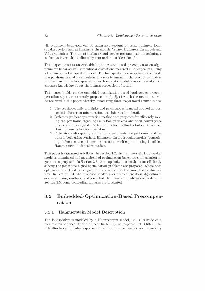
82 Chapter 3. Loudspeaker Precompensation
[4]. Nonlinear behaviour can be taken into account by using nonlinear loud-speaker models such as Hammerstein models, Wiener-Hammerstein models andVolterra models. The aim of nonlinear loudspeaker precompensation techniquesis then to invert the nonlinear system under consideration [5].
This paper presents an embedded-optimization-based precompensation algo-rithm for linear as well as nonlinear distortions incurred in loudspeakers, usinga Hammerstein loudspeaker model. The loudspeaker precompensation consistsin a per-frame signal optimization. In order to minimize the perceptible distor-tion incurred in the loudspeaker, a psychoacoustic model is incorporated whichcaptures knowledge about the human perception of sound.
This paper builds on the embedded-optimization-based loudspeaker precom-pensation algorithms recently proposed in [6]-[7], of which the main ideas willbe reviewed in this paper, thereby introducing three major novel contributions:
1. The psychoacoustic principles and psychoacoustic model applied for per-ceptible distortion minimization are elaborated in detail.
2. Different gradient optimization methods are proposed for efficiently solv-ing the per-frame signal optimization problems and their convergenceproperties are analyzed. Each optimization method is tailored to a givenclass of memoryless nonlinearities.
3. Extensive audio quality evaluation experiments are performed and re-ported, both using synthetic Hammerstein loudspeaker models (compris-ing different classes of memoryless nonlinearities), and using identifiedHammerstein loudspeaker models.
This paper is organized as follows. In Section 3.2, the Hammerstein loudspeakermodel is introduced and an embedded-optimization-based precompensation al-gorithm is proposed. In Section 3.3, three optimization methods for efficientlysolving the per-frame signal optimization problems are proposed, where eachoptimization method is designed for a given class of memoryless nonlineari-ties. In Section 3.4, the proposed loudspeaker precompensation algorithm isevaluated using synthetic and identified Hammerstein loudspeaker models. InSection 3.5, some concluding remarks are presented.
3.2 Embedded-Optimization-Based Precompen-
sation
3.2.1 Hammerstein Model Description
The loudspeaker is modeled by a Hammerstein model, i.e. a cascade of amemoryless nonlinearity and a linear finite impulse response (FIR) filter. TheFIR filter has an impulse response h[n], n = 0...L. The memoryless nonlinearity

3.2. Embedded-Optimization-Based Precompensation 83
g(x) is represented as a linear combination of P basis functions,
g(x) =P∑
p=1
cpψp(x) = ψT (x)c (3.1)
where the basis functions are stacked in a vector ψ(x) = [ψ1(x), ..., ψP (x)]T
and the corresponding coefficients are stacked in a vector c = [c1, ..., cP ]T .
A per-frame processing of the digital input audio signal x[n] will be applied,employing input frames xm = [xm,1, ..., xm,N ]T ∈ R
N ,m = 0, 1...M , with N ≥L, and xm,i = x[mN + i]. The output g(xm) of the memoryless nonlinearityfor a given input frame xm is straightforwardly constructed using the relation(3.1),
g(xm) = [g(xm,1), ..., g(xm,N )]T
= Ψ(xm)c (3.2)
where the basis function vectors for the different samples are assembled in amatrix Ψ(xm) = [ψ(xm,1), ...,ψ(xm,N )]T .
The output frame ym of the Hammerstein model can then be written as
ym = Hmg(xm) + Hmg(xm−1) (3.3)
where the matrices Hm ∈ RN×N and Hm ∈ RN×N implement a convolutionoperation with the FIR filter h[n] as follows,
Hm =
h[0] 0 . . . . . . . . . . . . 0h[1] h[0] 0 . . . . . . . . . 0...
. . .. . .
. . ....
h[L]. . .
. . .. . .
...
0. . .
. . .. . .
. . ....
.... . .
. . .. . .
. . . 00 . . . 0 h[L] . . . h[1] h[0]
(3.4)
Hm =
0 . . . 0 h[L] . . . h[2] h[1]0 . . . 0 0 h[L] . . . h[2]...
. . .. . .
......
. . . h[L]... 0...
...0 0 . . . . . . . . . . . . 0
. (3.5)

84 Chapter 3. Loudspeaker Precompensation
Optimization problem
solver
Psychoacoustic
model
LOUDSPEAKER
COMPENSATIONHAMMERSTEIN
LOUDSPEAKER MODEL
Figure 3.1: Embedded-optimization-based precompensation: schematicoverview.
3.2.2 Embedded-Optimization-Based Precompensation
Figure 3.1 shows the operation of the proposed embedded-optimization-basedloudspeaker precompensation technique. Before it is fed into the loudspeaker,the input frame xm passes through the loudspeaker precompensation block.For a given input frame xm, the loudspeaker precompensation consists of thefollowing steps:
1. Calculate the global masking threshold tm ∈ RN2 +1 of the input frame
xm using a psychoacoustic model (see Subsection 3.2.3).2. Calculate a precompensated input frame v∗
m ∈ RN as the solution of anoptimization problem, such that the corresponding output frame y∗
m isperceptually as close as possible to xm.
The precompensated input frame v∗m is calculated from the knowledge of the
input frame xm and its masking threshold tm. The objective function reflectsthe amount of perceptible distortion added between ym and xm,
v∗m = argmin
vm∈RN
1
2N
N−1∑
i=0
wm,i|Ym(ejωi)−Xm(ejωi)|2 (3.6)
where ωi = (2πi)/N represents the discrete frequency variable, Xm(ejωi) andYm(ejωi) are the discrete frequency components of xm and ym respectively, andwm,i are the strictly positive weights of a perceptual weighting function wm =[wm,0, ..., wm,N−1]
T ∈ RN . The perceptual weighting function depends on themasking threshold tm and is obeing the symmetry property wm,i = wm,N−i fori = 1, 2, ..., N2 − 1 (see subsection 3.2.3).
Optimization problem (3.6) can then be rewritten as
v∗m = argmin
vm∈RN
1
2(ym − xm)T DHWmD
︸ ︷︷ ︸
,Qm
(ym − xm) (3.7)
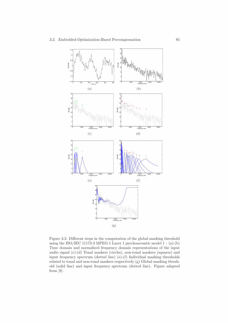
3.2. Embedded-Optimization-Based Precompensation 85
0 100 200 300 400 500−0.15
−0.1
−0.05
0
0.05
0.1
0.15
Time (n)
Am
plit
ude
(a)
0 5000 10000 15000 20000−10
0
10
20
30
40
50
60
Frequency (Hz)
SP
L(d
B)
(b)
0 5000 10000 15000 20000−10
0
10
20
30
40
50
60
Frequency (Hz)
SP
L(d
B)
(c)
0 5000 10000 15000 20000−10
0
10
20
30
40
50
60
Frequency (Hz)
SP
L(d
B)
(d)
0 5000 10000 15000 20000−10
0
10
20
30
40
50
60
Frequency (Hz)
SP
L(d
B)
(e)
0 5000 10000 15000 20000−10
0
10
20
30
40
50
60
Frequency (Hz)
SP
L(d
B)
(f)
0 5000 10000 15000 20000−10
0
10
20
30
40
50
60
Frequency (Hz)
SP
L(d
B)
(g)
Figure 3.2: Different steps in the computation of the global masking thresholdusing the ISO/IEC 11172-3 MPEG-1 Layer 1 psychoacoustic model 1 : (a)-(b)Time domain and normalized frequency domain representations of the inputaudio signal (c)-(d) Tonal maskers (circles), non-tonal maskers (squares) andinput frequency spectrum (dotted line) (e)-(f) Individual masking thresholdsrelated to tonal and non-tonal maskers respectively (g) Global masking thresh-old (solid line) and input frequency spectrum (dotted line). Figure adaptedfrom [8].
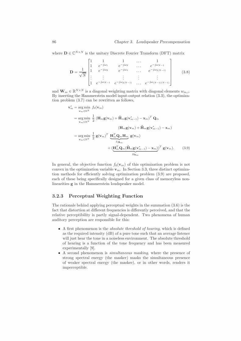
86 Chapter 3. Loudspeaker Precompensation
where D ∈ CN×N is the unitary Discrete Fourier Transform (DFT) matrix
D =1√N
1 1 1 . . . 11 e−jω1 e−jω2 . . . e−jωN−1
1 e−jω2 e−jω4 . . . e−jω2(N−1)
......
......
...1 e−jωN−1 e−jω2(N−1) . . . e−jω(N−1)(N−1)
(3.8)
and Wm ∈ RN×N is a diagonal weighting matrix with diagonal elements wm,i.By inserting the Hammerstein model input-output relation (3.3), the optimiza-tion problem (3.7) can be rewritten as follows,
v∗
m = argminvm∈RN
f0(vm)
= argminvm∈RN
1
2(Hmg(vm) + Hmg(v∗
m−1)− xm)T Qm
(Hmg(vm) + Hmg(v∗
m−1)− xm)
= argminvm∈RN
1
2g(vm)T H
TmQmHm
︸ ︷︷ ︸
,Am
g(vm)
+ (HTmQm(Hmg(v∗
m−1)− xm)︸ ︷︷ ︸
,bm
)T g(vm). (3.9)
In general, the objective function f0(vm) of this optimization problem is notconvex in the optimization variable vm. In Section 3.3, three distinct optimiza-tion methods for efficiently solving optimization problem (3.9) are proposed,each of these being specifically designed for a given class of memoryless non-linearities g in the Hammerstein loudspeaker model.
3.2.3 Perceptual Weighting Function
The rationale behind applying perceptual weights in the summation (3.6) is thefact that distortion at different frequencies is differently perceived, and that therelative perceptibility is partly signal-dependent. Two phenomena of humanauditory perception are responsible for this:
• A first phenomenon is the absolute threshold of hearing, which is definedas the required intensity (dB) of a pure tone such that an average listenerwill just hear the tone in a noiseless environment. The absolute thresholdof hearing is a function of the tone frequency and has been measuredexperimentally [9].
• A second phenomenon is simultaneous masking, where the presence ofstrong spectral energy (the masker) masks the simultaneous presenceof weaker spectral energy (the maskee), or in other words, renders itimperceptible.

3.2. Embedded-Optimization-Based Precompensation 87
Combining both phenomena, the instantaneous global masking threshold tmof the input audio signal xm gives the amount of signal energy (dB) at eachfrequency that can be masked by the signal. As such, the masking thresholdtm gives an indication of the relative perceptibility of signal components atdifferent frequencies.
Consider the input frame xm to act as the masker, and ym−xm as the maskee.By selecting the weights wm,i to be exponentially decreasing with the value ofthe global masking threshold tm of the signal xm at frequency i, i.e.
wm,i =
10−αtm,i if 0 ≤ i ≤ N
2
10−αtm,N−i if N2 < i ≤ N − 1
(3.10)
the objective function reflects the amount of perceptible distortion introduced.Appropriate values of the compression parameter α have been determined tolie in the range [0.01, 0.04].
The instantaneous global masking threshold tm of a given audio signal is cal-culated using part of the ISO/IEC 11172-3 MPEG-1 Layer 1 psychoacousticmodel 1. A complete description of the operation of this psychoacoustic modelis beyond the scope of this paper (we refer the reader to [10] and [11]). Weoutline the relevant steps [8] in the computation of tm and illustrate the resultof each step on an example audio signal (see Figure 3.2):
1. Spectral analysis and SPL normalization: In this step a high-resolutionspectral estimate of the audio signal is calculated, with spectral compo-nents expressed in terms of sound pressure level (SPL). After a normal-ization operation and a Hann windowing operation on the input signalframe, the PSD estimate is obtained through a 512-point DFT. Fig-ure 3.2(a) shows the time-domain input signal, Figure 3.2(b) shows theresulting spectral estimate.
2. Identification of tonal and non-tonal maskers : It is known from psy-choacoustic research that the tonality of a masking component has aninfluence on its masking properties [12]. For this reason it is importantto discriminate between tonal maskers (defined as local maxima of thesignal spectrum) and non-tonal maskers. The output of the DFT is usedto determine the relevant tonal and non-tonal maskers in the spectrumof the audio signal. In a first phase, tonal maskers are identified atlocal maxima of the PSD: energy from three adjacent spectral compo-nents centered at the local maximum is combined to form a single tonalmasker. In a second phase, a single non-tonal masker per critical bandis formed by addition of all the energy from the spectral componentswithin the critical band that have not contributed to a tonal masker.
3. Decimation of maskers : In this step, the number of maskers is reducedusing two criteria. First, any tonal or non-tonal masker below the ab-solute threshold of hearing is discarded. Next, any pair of maskers oc-curring within a distance of 0.5 Bark is replaced by the stronger of the

88 Chapter 3. Loudspeaker Precompensation
two. Figures 3.2(c) and 3.2(d) depict the identified tonal and non-tonalmaskers respectively, after decimation.
4. Calculation of individual masking thresholds : an individual maskingthreshold is calculated for each masker in the decimated set of tonaland non-tonal maskers, using fixed psychoacoustic rules. Essentially,the individual masking threshold depends on the frequency, loudnesslevel and tonality of the masker. Figure 3.2(e) and 3.2(f) show the indi-vidual masking thresholds associated with tonal and non-tonal maskers,respectively.
5. Calculation of global masking threshold : Finally, the global maskingthreshold is calculated by a power-additive combination of the tonal andnon-tonal individual masking thresholds, and the absolute threshold ofhearing. This is illustrated in Figure 3.2(g).
3.3 Optimization Methods
The efficient solution of the per-frame optimization problem (3.9) is crucial forthe proposed loudspeaker precompensation algorithm to be applicable in real-time environments. In this section, three optimization methods for efficientlysolving the considered optimization problem are proposed, each optimizationmethod being specifically designed for a given class of memoryless nonlinearitiesg in the Hammerstein loudspeaker model.
3.3.1 Classes of Memoryless Nonlinearities
In order to define the considered classes of memoryless nonlinearities, the no-tions of invertibility and smoothness for memoryless nonlinearities are firstintroduced.
Definition 3.1 [Invertible memoryless nonlinearity] A memoryless nonlinearityy = g(x) is invertible on the domain D ⊆ R if there exists a unique functionx = g−1(y) for which
g−1(g(x)) = x, ∀ x ∈ D. (3.11)
The function g−1(y) is called the inverse memoryless nonlinearity of g(x) onthe domain D. The output g−1(ym) of the inverse memoryless nonlinearity fora given frame ym is constructed as
g−1(ym) = [g−1(ym,1), ..., g−1(ym,N )]T . (3.12)
2

3.3. Optimization Methods 89
Definition 3.2 [Smooth memoryless nonlinearity] A memoryless nonlinearityy = g(x) is smooth on the domain D ⊆ R if its derivatives of all orders existand are continuous on D. 2
Based on the above definitions, the following three classes of memoryless non-linearities1 can be determined:
• Class I is formed by the invertible memoryless nonlinearities, such as theone depicted in Figure 3.3(a).
• Class II is formed by the non-invertible smooth memoryless nonlineari-ties, such as the one depicted in Figure 3.3(b).
• Class III is formed by the non-invertible non-smooth hard clipping mem-oryless nonlinearities, such as the one depicted in Figure 3.3(c). Thisclass of memoryless nonlinearities has a characteristic of the form
g(x) =
x, |x| ≤ Usgn(x)U, |x| > U
(3.13)
with U defined as the clipping level.
For each of these classes of memoryless nonlinearities, a specific optimizationmethod is proposed for solving the optimization problem (3.9) in a fast andreliable way.
3.3.2 Class I: Invertible Memoryless Nonlinearities
In case the memoryless nonlinearity g in the Hammerstein model is invertible,the precompensation of the linear FIR filter h and the precompensation ofthe memoryless nonlinearity g can be decoupled. In a first step, the linear FIRfilter can be precompensated for, resulting in the nonlinearly transformed frameg(v∗
m). In a second step, the memoryless nonlinearity g can be precompensatedfor by applying the inverse memoryless nonlinearity g−1 to g(v∗
m) in order tocompute the precompensated input frame v∗
m, i.e.
v∗m = g−1(g(v∗
m)). (3.14)
In order to carry out the first precompensation step, the objective function in(3.9) can be seen to be a strictly convex quadratic function of the nonlinearlytransformed variable g(vm), i.e.
g(v∗m) = argmin
g(vm)∈RN
f1(g(vm))
1In the remainder of this paper, all considered memoryless nonlinearities are assumed tooperate on the domain D = [−1, 1].
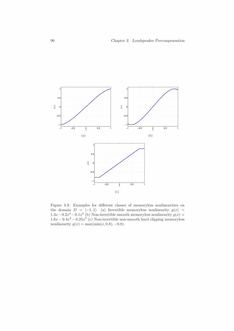
90 Chapter 3. Loudspeaker Precompensation
−1 −0.5 0 0.5 1
−1
−0.5
0
0.5
1
x
g(x
)
(a)
−1 −0.5 0 0.5 1
−1
−0.5
0
0.5
1
x
g(x
)
(b)
−1 −0.5 0 0.5 1
−1
−0.5
0
0.5
1
x
g(x
)
(c)
Figure 3.3: Examples for different classes of memoryless nonlinearities onthe domain D = [−1, 1]: (a) Invertible memoryless nonlinearity g(x) =1.3x−0.2x3−0.1x5 (b) Non-invertible smooth memoryless nonlinearity g(x) =1.6x− 0.4x3 − 0.25x5 (c) Non-invertible non-smooth hard clipping memorylessnonlinearity g(x) = max(min(x, 0.8),−0.8).

3.3. Optimization Methods 91
= argming(vm)∈RN
1
2g(vm)T Am g(vm) + bT
m g(vm) (3.15)
with Am ≻ 0. Indeed, as it was shown that Qm ≻ 0 in [8], it follows thatAm = HT
mQmHm ≻ 0, since congruence transformations have the property ofpreserving positive definiteness.
The necessary and sufficient condition for g(v∗m) to be the unique global min-
imizer of this strictly convex optimization problem, is
∇f1(g(v∗m)) = 0 (3.16)
from which the following closed form solution g(v∗m) can be derived,
g(v∗m) = −A−1
m bm
= −(HTmQmHm)−1(HT
mQm(Hmg(v∗m−1)− xm))
= −H−1m (Hmg(v∗
m−1)− xm) (3.17)
where the symmetry of Qm is used and the invertibility of Hm is assumed toestablish the last equality. It can be easily shown that f1(g(v
∗m)) = 0, implying
that a perfect precompensation y∗m = xm is achieved. Note that the perceptual
weighting Wm of the frequency domain error terms (which are all zero in thesolution) is unable to affect this solution, explaining the absence of Qm in(3.17).
3.3.3 Class II: Non-Invertible Smooth Memoryless Non-
linearities
In case the memoryless nonlinearity g in the Hammerstein model is non-invertible, the precompensation of the linear FIR filter h and the precompen-sation of the memoryless nonlinearity g should be performed simultaneouslyby solving optimization problem (3.9). From the smoothness property of g andits constituting basis functions ψ, it follows that for any xm ∈ DN the gradient∇g(xm) ∈ RN can be computed as
∇g(xm) = [∇g(xm,1), ...,∇g(xm,N )]T
= ∇Ψ(xm)c (3.18)
where the matrix ∇Ψ(xm) ∈ RN×P is defined as
∇Ψ(xm) =
∇ψ1(xm,1) . . . ∇ψP (xm,1)...
. . ....
∇ψ1(xm,N ) . . . ∇ψP (xm,N )
. (3.19)
The proposed optimization method for solving the non-convex optimizationproblem (3.9) is an iterative gradient method. Introducing the notation vk
m for

92 Chapter 3. Loudspeaker Precompensation
the kth iterate of the mth frame, the (k+1)th iteration of the iterative gradientmethod consists in taking a step along the negative gradient direction,
vk+1m = vk
m − skm∇f0(vkm) (3.20)
where skm is the stepsize and the gradient ∇f0(vkm) is computed as
∇f0(vkm) = diag(∇g(vk
m))
[
HTmQm
(
Hmg(vkm)
+Hmg(v∗m−1)− xm
)]
(3.21)
and where ∇g(vkm) is established using (3.18)-(3.19).
The stepsize skm is determined using a backtracking line search for satisfyingthe Armijo sufficient decrease condition [13],
f0(vkm − skm∇f0(vk
m)) ≤ f0(vkm)− βskm‖∇f0(vk
m)‖22 (3.22)
with β ∈ (0, 12 ) the relaxation of the gradient. Starting from skm = 1, successivereductions of skm by a factor η ∈ (0, 1) are performed until the condition (3.22)holds. The resulting algorithm is given in Algorithm 4.
3.3.4 Class III: Non-Invertible Hard Clipping Memory-
less Nonlinearities
In case the memoryless nonlinearity g in the Hammerstein model is a non-invertible hard clipping memoryless nonlinearity with clipping level U as de-fined in (3.13), optimization problem (3.9) can be rewritten as follows,
v∗m = argmin
vm∈RN
f1(vm) s.t. −u ≤ vm ≤ u
= argminvm∈RN
1
2vTm Am vm + bT
m vm
s.t. −u ≤ vm ≤ u (3.23)
where u = U1N contains the per-sample clipping levels and 1N ∈ RN is an allones vector. Note that by constraining vm to be within the linear range [−U,U ]of the memoryless nonlinearity g, it is possible to introduce the equivalenceg(vm) = vm in the objective function. The strictly convex quadratic objectivefunction (Am ≻ 0) and the affine constraints make optimization problem (3.23)a strictly convex quadratic program.
The proposed optimization method for solving the strictly convex optimizationproblem (3.23) is an iterative projected gradient method. In each iteration ofa projected gradient method, first a step is taken along the negative gradi-ent direction of the objective function, after which the result is orthogonally
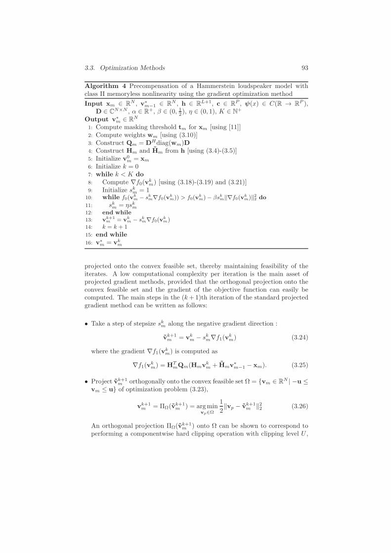
3.3. Optimization Methods 93
Algorithm 4 Precompensation of a Hammerstein loudspeaker model withclass II memoryless nonlinearity using the gradient optimization method
Input xm ∈ RN , v∗
m−1 ∈ RN , h ∈ R
L+1, c ∈ RP , ψ(x) ∈ C(R → R
P ),D ∈ CN×N , α ∈ R+, β ∈ (0, 12 ), η ∈ (0, 1), K ∈ N+
Output v∗m ∈ RN
1: Compute masking threshold tm for xm [using [11]]2: Compute weights wm [using (3.10)]3: Construct Qm = DHdiag(wm)D4: Construct Hm and Hm from h [using (3.4)-(3.5)]5: Initialize v0
m = xm
6: Initialize k = 07: while k < K do8: Compute ∇f0(vk
m) [using (3.18)-(3.19) and (3.21)]9: Initialize skm = 1
10: while f0(vkm − skm∇f0(v
km)) > f0(v
km)− βskm‖∇f0(v
km)‖22 do
11: skm = ηskm12: end while
13: vk+1m = vk
m − skm∇f0(vkm)
14: k = k + 1
15: end while16: v∗
m = vkm
projected onto the convex feasible set, thereby maintaining feasibility of theiterates. A low computational complexity per iteration is the main asset ofprojected gradient methods, provided that the orthogonal projection onto theconvex feasible set and the gradient of the objective function can easily becomputed. The main steps in the (k+1)th iteration of the standard projectedgradient method can be written as follows:
• Take a step of stepsize skm along the negative gradient direction :
vk+1m = vk
m − skm∇f1(vkm) (3.24)
where the gradient ∇f1(vkm) is computed as
∇f1(vkm) = HT
mQm(Hmvkm + Hmv∗
m−1 − xm). (3.25)
• Project vk+1m orthogonally onto the convex feasible set Ω = vm ∈ RN | −u ≤
vm ≤ u of optimization problem (3.23),
vk+1m = ΠΩ(v
k+1m ) = argmin
vp∈Ω
1
2‖vp − vk+1
m ‖22 (3.26)
An orthogonal projection ΠΩ(vk+1m ) onto Ω can be shown to correspond to
performing a componentwise hard clipping operation with clipping level U ,
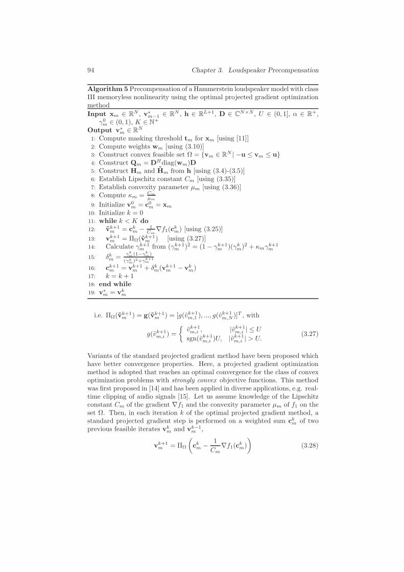
94 Chapter 3. Loudspeaker Precompensation
Algorithm 5 Precompensation of a Hammerstein loudspeaker model with classIII memoryless nonlinearity using the optimal projected gradient optimizationmethod
Input xm ∈ RN , v∗m−1 ∈ RN , h ∈ RL+1, D ∈ CN×N , U ∈ (0, 1], α ∈ R+,
γ0m ∈ (0, 1), K ∈ N+
Output v∗m ∈ RN
1: Compute masking threshold tm for xm [using [11]]2: Compute weights wm [using (3.10)]3: Construct convex feasible set Ω = vm ∈ RN | −u ≤ vm ≤ u4: Construct Qm = DHdiag(wm)D5: Construct Hm and Hm from h [using (3.4)-(3.5)]6: Establish Lipschitz constant Cm [using (3.35)]7: Establish convexity parameter µm [using (3.36)]8: Compute κm = Cm
µm
9: Initialize v0m = c0m = xm
10: Initialize k = 011: while k < K do12: vk+1
m = ckm − 1Cm
∇f1(ckm) [using (3.25)]
13: vk+1m = ΠΩ(v
k+1m ) [using (3.27)]
14: Calculate γk+1m from (γk+1
m )2 = (1− γk+1m )(γkm)2 + κmγ
k+1m
15: δkm =γkm(1−γk
m)
(γkm)2+γ
k+1m
16: ck+1m = vk+1
m + δkm(vk+1m − vk
m)17: k = k + 118: end while19: v∗
m = vkm
i.e. ΠΩ(vk+1m ) = g(vk+1
m ) = [g(vk+1m,1 ), ..., g(v
k+1m,N )]T , with
g(vk+1m,i ) =
vk+1m,i , |vk+1
m,i | ≤ U
sgn(vk+1m,i )U, |vk+1
m,i | > U.(3.27)
Variants of the standard projected gradient method have been proposed whichhave better convergence properties. Here, a projected gradient optimizationmethod is adopted that reaches an optimal convergence for the class of convexoptimization problems with strongly convex objective functions. This methodwas first proposed in [14] and has been applied in diverse applications, e.g. real-time clipping of audio signals [15]. Let us assume knowledge of the Lipschitzconstant Cm of the gradient ∇f1 and the convexity parameter µm of f1 on theset Ω. Then, in each iteration k of the optimal projected gradient method, astandard projected gradient step is performed on a weighted sum ckm of twoprevious feasible iterates vk
m and vk−1m ,
vk+1m = ΠΩ
(
ckm − 1
Cm
∇f1(ckm)
)
(3.28)

3.3. Optimization Methods 95
where
ckm = vkm + δkm(vk
m − vk−1m ) (3.29)
where δkm is computed as
δkm =γk−1m (1 − γk−1
m )
(γk−1m )2 + γkm
(3.30)
and where γkm is computed as the solution of
(γkm)2 = (1 − γkm)(γk−1m )2 + κmγ
km (3.31)
and κm = Cm
µmis the condition number.
In order to establish Cm and µm for optimization problem (3.23), the next twolemmas are proposed.
Lemma 3 ([14]) Let function f1 be twice continuously differentiable on set Ω.The gradient ∇f1 is Lipschitz continuous on set Ω with Lipschitz constant Cif and only if
∇2f1(z) CI , ∀z ∈ Ω (3.32)
Lemma 4 ([14]) Let function f1 be twice continuously differentiable on set Ω.The function f1 is strongly convex on set Ω with convexity parameter µ if andonly if there exists µ > 0 such that
∇2f1(z) µI , ∀z ∈ Ω (3.33)
Let us denote and order the eigenvalues of Am as follows,
λ1(Am) ≤ λ2(Am) ≤ · · · ≤ λN−1(Am) ≤ λN (Am). (3.34)
Using Lemma 3.1 and Lemma 3.2, it is then shown that the Lipschitz constantCm can be computed as the largest eigenvalue of Am,
Cm = λN (Am) = λN (HTmQmHm) (3.35)
and that the convexity parameter µm can be computed as the smallest eigen-value of Am,
µm = λ1(Am) = λ1(HTmQmHm). (3.36)
The resulting algorithm is given as Algorithm 5.

96 Chapter 3. Loudspeaker Precompensation
3.3.5 Algorithmic Complexity Bounds
It is possible to derive polynomial upper and lower bounds on the algorithmiccomplexity, i.e. the number of necessary iterations of the optimization methodproposed in subsection 3.3.4 as a function of the solution accuracy. For theclass of convex optimization problems with strongly convex objective functions,bounds on the algorithmic complexity of the projected gradient method usedin Algorithm 5 are derived as follows:
Theorem 3.3 ([14]) Let f1 be a strongly convex, continuously differentiablefunction with Lipschitz constant Cm and convexity parameter µm = Cm
κm(where
the condition number κm > 1), and let Ω be a convex feasible set. Then theminimum and maximum number of necessary iterations of the optimal pro-jected gradient method described in Algorithm 5 to find a solution vk
m satisfyingf1(v
km)− f1(v
∗m) ≤ ǫ are given by
kminm =
√κm − 1
4log
(µm||v0
m − v∗m||2
2ǫ
)
(3.37)
kmaxm =
√κm log
(Cm||v0
m − v∗m||2
ǫ
)
. (3.38)
It has been shown that congruence transformations like Qm → HTmQmHm do
preserve the signs but not the magnitudes of the matrix eigenvalues. Interest-ingly, bounds on the change in magnitude of the eigenvalues under a congruencetransformation have been established,
Theorem 3.4 ([16]) Let Qm ∈ RN×N be symmetric and Hm ∈ RN×N nonsin-gular. Let the eigenvalues of Qm and HT
mQmHm be arranged in nondecreasingorder (3.34). Let σ1(Hm) ≥ · · · ≥ σN (Hm) > 0 be the singular values of Hm.Then each eigenvalue λi(H
TmQmHm), i = 1, ..., N , is bounded as follows,
σ2N (Hm)λi(Qm) ≤ λi(H
TmQmHm) ≤ σ2
1(Hm)λi(Qm). (3.39)
Corollary 3.5 The condition number κ(HTmQmHm) =
λN (HTmQmHm)
λ1(HTmQmHm)
is bounded
as follows,
κ(HTmQmHm) ≥ max
(1, κ−1(HT
mHm)κ(Qm))
(3.40)
κ(HTmQmHm) ≤ κ(HT
mHm)κ(Qm). (3.41)
The previous theorem and its corollary now allow to rewrite the lower andupper iteration bounds (3.37)-(3.38) as a function of the extreme eigenvaluesand singular values of Hm and Qm.
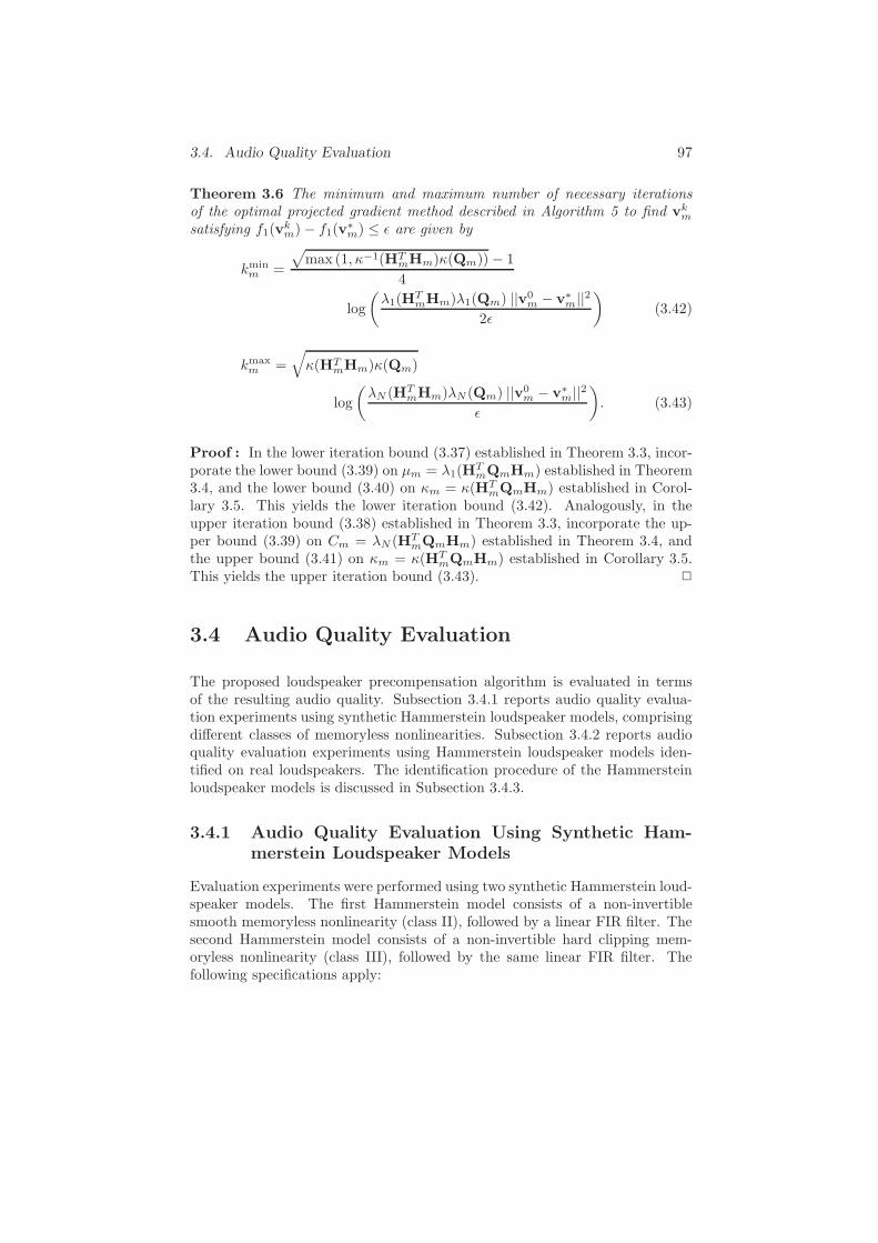
3.4. Audio Quality Evaluation 97
Theorem 3.6 The minimum and maximum number of necessary iterationsof the optimal projected gradient method described in Algorithm 5 to find vk
m
satisfying f1(vkm)− f1(v
∗m) ≤ ǫ are given by
kminm =
√
max (1, κ−1(HTmHm)κ(Qm))− 1
4
log
(λ1(H
TmHm)λ1(Qm) ||v0
m − v∗m||2
2ǫ
)
(3.42)
kmaxm =
√
κ(HTmHm)κ(Qm)
log
(λN (HT
mHm)λN (Qm) ||v0m − v∗
m||2ǫ
)
. (3.43)
Proof : In the lower iteration bound (3.37) established in Theorem 3.3, incor-porate the lower bound (3.39) on µm = λ1(H
TmQmHm) established in Theorem
3.4, and the lower bound (3.40) on κm = κ(HTmQmHm) established in Corol-
lary 3.5. This yields the lower iteration bound (3.42). Analogously, in theupper iteration bound (3.38) established in Theorem 3.3, incorporate the up-per bound (3.39) on Cm = λN (HT
mQmHm) established in Theorem 3.4, andthe upper bound (3.41) on κm = κ(HT
mQmHm) established in Corollary 3.5.This yields the upper iteration bound (3.43). 2
3.4 Audio Quality Evaluation
The proposed loudspeaker precompensation algorithm is evaluated in termsof the resulting audio quality. Subsection 3.4.1 reports audio quality evalua-tion experiments using synthetic Hammerstein loudspeaker models, comprisingdifferent classes of memoryless nonlinearities. Subsection 3.4.2 reports audioquality evaluation experiments using Hammerstein loudspeaker models iden-tified on real loudspeakers. The identification procedure of the Hammersteinloudspeaker models is discussed in Subsection 3.4.3.
3.4.1 Audio Quality Evaluation Using Synthetic Ham-
merstein Loudspeaker Models
Evaluation experiments were performed using two synthetic Hammerstein loud-speaker models. The first Hammerstein model consists of a non-invertiblesmooth memoryless nonlinearity (class II), followed by a linear FIR filter. Thesecond Hammerstein model consists of a non-invertible hard clipping mem-oryless nonlinearity (class III), followed by the same linear FIR filter. Thefollowing specifications apply:

98 Chapter 3. Loudspeaker Precompensation
Table
3.1:Audio
excerp
tsdatabase
used
forcomparativ
eaudio
quality
evaluatio
n(16bitmonoat44.1
kHz).
Nr.
Name
Texture
Compositio
nStyle
Duratio
n[s]
Sample
start
Sample
end
Orig
in1
poulen
c.wav
polyphonic
instru
mental
classica
l17.8
400000
1183000
[17]
2rhcp.wav
polyphonic
instru
mental
rock
9.8
468996
900000
[18]
3pierle.w
avpolyphonic
instru
mental+
vocal
pop
11.7
2234000
2750000
[19]
4chopin.wav
monophonic
instru
mental
classica
l17.8
50000
836200
[20]
5kraftw
.wav
polyphonic
instru
mental
electronic
17.2
7480000
8240000
[21]
6crefsa
x.wav
monophonic
instru
mental
classica
l10.9
1479026
[22]
7grefcla
.wav
monophonic
instru
mental
classica
l6.9
1302534
[22]
8arefcla
.wav
monophonic
instru
mental
classica
l7.4
1302534
[22]

3.4. Audio Quality Evaluation 99
• Class II memoryless nonlinearity: P = 3 basis functionsψ(x) = [x x3 x5]T ,a corresponding coefficient vector c = [1.6 − 0.4 − 0.25]T , depicted inFigure 3.3(b).
• Class III memoryless nonlinearity: of the form (3.13), with clipping levelU = 0.8, depicted in Figure 3.3(c).
• Linear FIR filter: L = 128, impulse response h[n], designed using the fre-quency sampling method fir2 in Matlab, having a required magnituderesponse [1 0.95 0.75 0.50 0.20 0]T for the frequencies [0 0.2 0.4 0.6 0.8 1]T×fNyquist.
A test database consisting of 8 audio excerpts was compiled (see Table 3.1 fordetails). Each audio signal in the test database was fed into each of the consid-ered Hammerstein loudspeaker models, once with and once without performingprecompensation. The following settings were used in the precompensation:
• First Hammerstein model: precompensation using Algorithm 4, withN = 512, α = 0.01, β = 0.1, η = 0.6, and K = 500.
• Second Hammerstein model: precompensation using Algorithm 5, with
N = 512, α = 0.01, γ0m =√
µm
Cm, and K = 500.
The objective audio quality improvement for each audio signal was assessed bycomputing the ∆ODG measure,
∆ODG = ODG(x,y∗)−ODG(x,y) (3.44)
where x is the input signal, y is the output signal when no precompensa-tion is applied, y∗ is the output signal when precompensation is applied, andODG(r,d) is an objective measure [22] that predicts the audio quality of a sig-nal d with respect to a signal r on a scale of [0,−4], where 0 corresponds to animperceptible degradation, and -4 corresponds to a very annoying degradation.
The simulations were performed for four distinct average amplitude levels of theinput signals, selected such that the corresponding ODG(x,y) = −0.5,−1.0,−1.5,−2.0. This signal-specific selection of the average amplitude levels en-sures a uniform audio quality degradation for different output signals when noprecompensation is applied.
The resulting ∆ODG scores for the first and second Hammerstein models areshown in Figure 3.4 and Figure 3.5, respectively. For the first Hammersteinmodel in Figure 3.4, a positive audio quality improvement is observed for allaudio excerpts, and this for all but one considered average amplitude level. Formost audio excerpts, increasing audio quality improvement scores are observedfor increasing average amplitude levels. Indeed, it is exactly at higher amplitudelevels that the Hammerstein memoryless nonlinearity is severely affecting theaudio signal, and that precompensation is capable of improving the resultingaudio quality considerably.
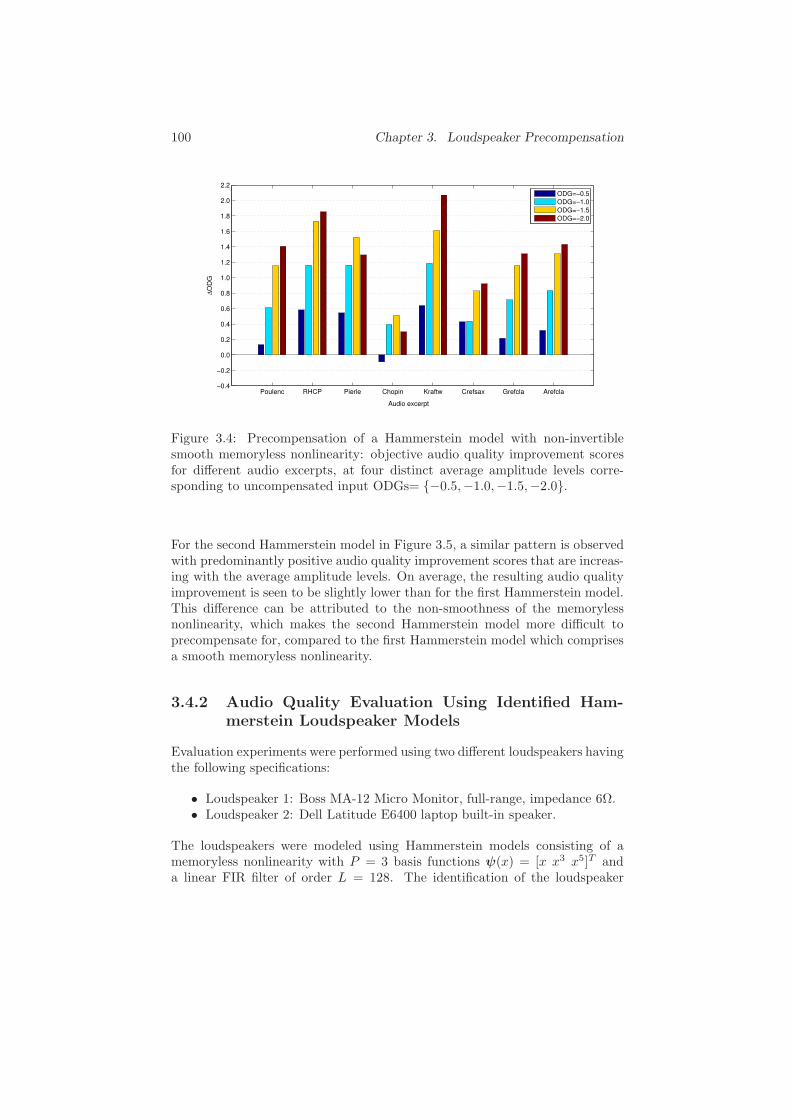
100 Chapter 3. Loudspeaker Precompensation
Poulenc RHCP Pierle Chopin Kraftw Crefsax Grefcla Arefcla−0.4
−0.2
0.0
0.2
0.4
0.6
0.8
1.0
1.2
1.4
1.6
1.8
2.0
2.2
Audio excerpt
∆O
DG
ODG=−0.5
ODG=−1.0
ODG=−1.5
ODG=−2.0
Figure 3.4: Precompensation of a Hammerstein model with non-invertiblesmooth memoryless nonlinearity: objective audio quality improvement scoresfor different audio excerpts, at four distinct average amplitude levels corre-sponding to uncompensated input ODGs= −0.5,−1.0,−1.5,−2.0.
For the second Hammerstein model in Figure 3.5, a similar pattern is observedwith predominantly positive audio quality improvement scores that are increas-ing with the average amplitude levels. On average, the resulting audio qualityimprovement is seen to be slightly lower than for the first Hammerstein model.This difference can be attributed to the non-smoothness of the memorylessnonlinearity, which makes the second Hammerstein model more difficult toprecompensate for, compared to the first Hammerstein model which comprisesa smooth memoryless nonlinearity.
3.4.2 Audio Quality Evaluation Using Identified Ham-
merstein Loudspeaker Models
Evaluation experiments were performed using two different loudspeakers havingthe following specifications:
• Loudspeaker 1: Boss MA-12 Micro Monitor, full-range, impedance 6Ω.• Loudspeaker 2: Dell Latitude E6400 laptop built-in speaker.
The loudspeakers were modeled using Hammerstein models consisting of amemoryless nonlinearity with P = 3 basis functions ψ(x) = [x x3 x5]T anda linear FIR filter of order L = 128. The identification of the loudspeaker
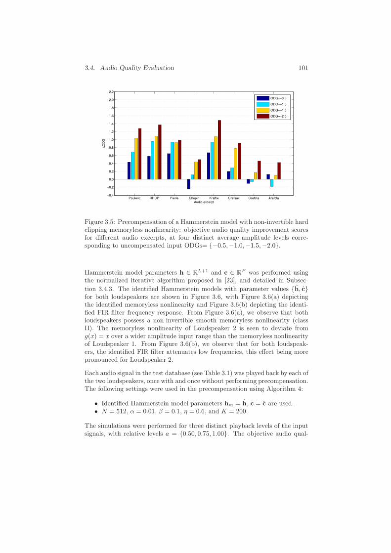
3.4. Audio Quality Evaluation 101
Poulenc RHCP Pierle Chopin Kraftw Crefsax Grefcla Arefcla−0.4
−0.2
0.0
0.2
0.4
0.6
0.8
1.0
1.2
1.4
1.6
1.8
2.0
2.2
Audio excerpt
∆O
DG
ODG=−0.5
ODG=−1.0
ODG=−1.5
ODG=−2.0
Figure 3.5: Precompensation of a Hammerstein model with non-invertible hardclipping memoryless nonlinearity: objective audio quality improvement scoresfor different audio excerpts, at four distinct average amplitude levels corre-sponding to uncompensated input ODGs= −0.5,−1.0,−1.5,−2.0.
Hammerstein model parameters h ∈ RL+1 and c ∈ RP was performed usingthe normalized iterative algorithm proposed in [23], and detailed in Subsec-
tion 3.4.3. The identified Hammerstein models with parameter values h, cfor both loudspeakers are shown in Figure 3.6, with Figure 3.6(a) depictingthe identified memoryless nonlinearity and Figure 3.6(b) depicting the identi-fied FIR filter frequency response. From Figure 3.6(a), we observe that bothloudspeakers possess a non-invertible smooth memoryless nonlinearity (classII). The memoryless nonlinearity of Loudspeaker 2 is seen to deviate fromg(x) = x over a wider amplitude input range than the memoryless nonlinearityof Loudspeaker 1. From Figure 3.6(b), we observe that for both loudspeak-ers, the identified FIR filter attenuates low frequencies, this effect being morepronounced for Loudspeaker 2.
Each audio signal in the test database (see Table 3.1) was played back by each ofthe two loudspeakers, once with and once without performing precompensation.The following settings were used in the precompensation using Algorithm 4:
• Identified Hammerstein model parameters hm = h, c = c are used.• N = 512, α = 0.01, β = 0.1, η = 0.6, and K = 200.
The simulations were performed for three distinct playback levels of the inputsignals, with relative levels a = 0.50, 0.75, 1.00. The objective audio qual-

102 Chapter 3. Loudspeaker Precompensation
−1 −0.5 0 0.5 1
−1
−0.5
0
0.5
1
x
g(x
)
Loudspeaker 1
Loudspeaker 2
(a)
−60
−50
−40
−30
−20
−10
0
10
20
ω
20lo
g10
|H(e
jω)|
0 π4
π2
3π4
π
Loudspeaker 1
Loudspeaker 2
(b)
Figure 3.6: Identified Hammerstein models for Loudspeaker 1 (solid lines) andLoudspeaker 2 (dashed lines): (a) memoryless nonlinearity (b) FIR filter fre-quency response.
ity improvement for each audio signal was assessed by computing the ∆ODGmeasure,
∆ODG = ODG(x,y∗)−ODG(x,y) (3.45)
where x is the input signal, y is the loudspeaker output signal when no prec-ompensation is applied, and y∗ is the loudspeaker output signal when precom-pensation is applied.
The resulting ∆ODG scores for Loudspeaker 1 and Loudspeaker 2 are shownin Figure 3.7(a) and Figure 3.7(b), respectively. For Loudspeaker 1 in Figure3.7(a), positive audio quality improvement scores are observed for most audioexcerpts. Increasing audio quality improvement scores are observed for increas-ing playback levels. The negative improvement scores for audio excerps Chopin(all playback levels), Grefcla and Arefcla (low playback levels) seem to indicatethat there is a signal-specific threshold on the loudspeaker playback level be-low which performing precompensation is unnecessary and can even harm theresulting audio quality.
For Loudspeaker 2 in Figure 3.7(b), a similar pattern is observed with audioquality improvement scores that are increasing with the playback level. For thehighest playback level a = 1.00, all precompensated audio excerpts result inan improved audio quality score. For the lower playback level, positive audioquality improvement scores are observed, except for the audio excerpts Chopin,Grefcla and Arefcla mentioned previously.

3.4. Audio Quality Evaluation 103
Poulenc RHCP Pierle Chopin Kraftw Crefsax Grefcla Arefcla−0.6
−0.4
−0.2
0.0
0.2
0.4
0.6
0.8
1.0
1.2
1.4
1.6
1.8
2.0
Audio excerpt
∆O
DG
a=0.50
a=0.75
a=1.00
(a)
Poulenc RHCP Pierle Chopin Kraftw Crefsax Grefcla Arefcla−0.6
−0.4
−0.2
0.0
0.2
0.4
0.6
0.8
1.0
1.2
1.4
1.6
1.8
2.0
Audio excerpt
∆O
DG
a=0.50
a=0.75
a=1.00
(b)
Figure 3.7: Precompensation of two loudspeakers using Hammerstein loud-speaker models - objective audio quality improvement scores for different audioexcerpts, at average amplitude levels = 0.50, 0.75, 1.00: (a) Loudspeaker 1(b) Loudspeaker 2.

104 Chapter 3. Loudspeaker Precompensation
3.4.3 Identification of Hammerstein Model Parameters
The purpose of identification is to estimate the unknown Hammerstein modelparameters hL = [h1, ..., hL]
T (excluding h0) and c = [c1, ..., cP ]T based on
an observed output signal y = [y1, ..., yN ]T and an observed input signal x =[x1, ..., xN ]T . In our experimental set-up, we have used a test audio signalhaving 30 seconds duration as the loudspeaker input signal, and measured theloudspeaker output signal in a soundproof room using a microphone placed onthe axis of the loudspeaker at a distance of 10 centimeter. The estimation isdone by solving the following optimization problem,
hL, c = argminhL,c
f2(hL, c)
= argminhL,c
1
N
N∑
n=1
(yn − hT
L Ψ(xn) c)2
(3.46)
where xn = [xn−1, ..., xn−L]T and consequentlyΨ(xn) = [ψ(xn−1), ...,ψ(xn−L)]
T .
Given an initial estimate h0L 6= 0, the normalized iterative algorithm [23] solves
optimization problem (3.46) by performing the following steps in each iterationk:
1. An estimate ck is computed as the solution of the least-squares problem(3.46) for fixed hL = hk−1
L ,
ck = argminc∈RP
f2(hk−1L , c). (3.47)
2. An estimate hkL is computed as the solution of the least-squares problem
(3.46) for fixed c = ck,
hkL = argmin
hL∈RL
f2(hL, ck). (3.48)
3. A normalization is performed so that ||hkL|| = 1,
hkL =
ξkhkL
||hkL||
(3.49)
ck = ξkck||hkL|| (3.50)
where ξk = ±1 is the sign of the first non-zero entry of hkL.
3.5. Conclusions 105
3.5 Conclusions
In this paper, an embedded-optimization-based loudspeaker precompensationalgorithm using a Hammerstein loudspeaker model has been presented. Theloudspeaker precompensation consists in a per-frame signal optimization. Inorder to minimize the perceptible distortion incurred in the loudspeaker, a per-cepually meaningful optimization criterion has been constructed. Dependingon the invertibility and the smoothness of the memoryless nonlinearity, differ-ent first order optimization methods have been proposed for solving the per-frame optimization problems. Objective evaluation experiments using syntheticand identified loudspeaker models have shown that the proposed loudspeakerprecompensation algorithm provides a significant audio quality improvement,especially so at high playback levels.
Bibliography
[1] K. Lashkari, “A modified Volterra-Wiener-Hammerstein model for loud-speaker precompensation,” in Proc. 39th Asilomar Conf. Signals, Syst.Comput., Pacific Grove, CA, Oct. 2005, pp. 344–348.
[2] C.-T. Tan, B. C. J. Moore, and N. Zacharov, “The effect of nonlineardistortion on the perceived quality of music and speech signals,” J. AudioEng. Soc., vol. 51, no. 11, pp. 1012–1031, Nov. 2003.
[3] B. C. Moore, C.-T. Tan, N. Zacharov, and V.-V. Mattila, “Measuring andpredicting the perceived quality of music and speech subjected to combinedlinear and nonlinear distortion,” Journal of the Audio Engineering Society,vol. 52, no. 12, pp. 1228–1244, 2004.
[4] M. Karjalainen and T. Paatero, “Equalization of loudspeaker and room re-sponses using Kautz filters: Direct least squares design,” EURASIP Jour-nal on Advances in Signal Processing, vol. 2007, pp. 1–13, 2007.
[5] M. V. K. Shi, G. T. Zhou, “Compensation for nonlinearity in a Ham-merstein system using the coherence function with application to nonlin-ear acoustic echo cancellation,” IEEE Transactions on Signal processing,vol. 55, no. 12, pp. 5853–5858, 2007.
[6] B. Defraene, T. van Waterschoot, M. Diehl, and M. Moonen, “Perception-based nonlinear loudspeaker compensation through embedded convex op-timization,” in 2012 Proceedings of the 20th European Signal ProcessingConference (EUSIPCO), Bucharest, Romania, Aug. 2012, pp. 2472 –2476.
[7] ——, “Embedded-optimization-based loudspeaker compensation using ageneric Hammerstein loudspeaker model,” in 2013 Proceedings of the 21st

106 Bibliography
European Signal Processing Conference (EUSIPCO), Marrakech, Morocco,Sept. 2013.
[8] B. Defraene, T. van Waterschoot, H. J. Ferreau, M. Diehl, and M. Moo-nen, “Real-time perception-based clipping of audio signals using convexoptimization,” IEEE Transactions on Audio, Speech, and Language Pro-cessing, vol. 20, no. 10, pp. 2657 –2671, Dec. 2012.
[9] E. Terhardt, “Calculating virtual pitch,” Hearing Res., vol. 1, no. 2, pp.155 – 182, 1979.
[10] T. Painter and A. Spanias, “Perceptual coding of digital audio,” Proc.IEEE, vol. 88, no. 4, pp. 451–515, Apr. 2000.
[11] ISO/IEC, “11172-3 Information technology - Coding of moving picturesand associated audio for digital storage media at up to about 1.5 Mbit/s- Part 3: Audio,” 1993.
[12] E. Zwicker and H. Fastl, Psychoacoustics: facts and models, 2nd ed.Springer, 1999.
[13] L. Armijo, “Minimization of functions having lipschitz continuous firstpartial derivatives.” Pacific Journal of mathematics, vol. 16, no. 1, pp.1–3, 1966.
[14] Y. Nesterov, Introductory lectures on convex optimization. Springer, 2004.
[15] B. Defraene, T. van Waterschoot, M. Diehl, and M. Moonen, “A fast pro-jected gradient optimization method for real-time perception-based clip-ping of audio signals,” in Proc. ICASSP 2011, Prague, Czech Republic,May 2011, pp. 333–336.
[16] A. Ostrowski, “A quantitative formulation of Sylvester’s law of inertia,”Proceedings of the National Academy of Sciences of the United States ofAmerica, vol. 45, no. 5, p. 740, 1959.
[17] F. Poulenc, “Sonata for flute and piano (Cantilena),” French Flute Music,Naxos 8.557328, 2005.
[18] Red Hot Chili Peppers, “Californication,” Californication, Warner Bros.Records 9362473862, 1999.
[19] An Pierle & White Velvet, “Mexico,” An Pierle & White Velvet, PIASRecordings 941.0170.020, 2006.
[20] F. Chopin, “Waltz op. 69 no. 2,” Favourite Piano Works (Vladimir Ashke-nazy), Decca 02894448302, 1995.
[21] Kraftwerk, “Tour de France Etape 1,” Minimum-Maximum, EMI Music724356061620, 2005.

107
[22] International Telecommunications Union Recommendation BS.1387,“Method for objective measurements of perceived audio quality,” 1998.
[23] E.-W. Bai and D. Li, “Convergence of the iterative Hammerstein sys-tem identification algorithm,” Automatic Control, IEEE Transactions on,vol. 49, no. 11, pp. 1929–1940, 2004.

108 Bibliography

Chapter 4
Subjective Audio Quality
Evaluation
4.1 Introduction
In Chapter 2 and Chapter 3, novel embedded-optimization-based precompen-sation algorithms have been presented which incorporate a perceptual model.In Chapter 2, a perception-based clipping algorithm has been presented usingembedded convex optimization. In Chapter 3, a loudspeaker precompensationalgorithm has been presented using embedded optimization. Both algorithmshave been evaluated using objective measures of audio quality, such as PEAQ[1] and Rnonlin [2], for which significant improvements have been reported.In Subsection 2.4, it has been concluded from evaluation experiments that theperception-based clipping algorithm results in significantly higher objective au-dio quality scores than existing clipping techniques. In Subsection 3.4, it hasbeen concluded from experiments using synthetic and identified loudspeakermodels that the proposed loudspeaker precompensation algorithm provides asignificant objective audio quality improvement, especially at high playbacklevels.
The objective measures used in the evaluation experiments are predictive mod-els of the perceived audio quality. Taking a reference signal (i.e. the cleansignal) and a signal under test (i.e. the processed signal) as an input, theobjective measure of perceived audio quality is calculated through sequentialapplication of a human auditory model and a cognitive model. Resultingly, aperceived audio quality score is attributed to the processed signal with respectto the clean signal.
109
110 Chapter 4. Subjective Audio Quality Evaluation
Although considerable research efforts have been invested in the developmentand standardization of such objective audio quality measures, limits on theiraccuracy and applicability are inevitable. Firstly, a given objective audio qual-ity measure is applicable to assess the perceptibility of the particular class ofdistortions it was designed for, and care should be taken when applying themeasure to assess the perceptibility of other distortions. For example, PEAQwas designed to assess the perceptibility of degradations commonly encoun-tered in audio codecs. Secondly, the current objective audio quality measuresare predictive models with a limited accuracy, and as a result cannot replacethe subjective evaluation of human listeners [3].
For these reasons, it is necessary to perform a formal subjective evaluation toaccurately measure the perceived audio quality for the algorithms presented inChapter 2 and Chapter 3. The subjective evaluation takes the form of a formallistening test, in which it is assessed how listeners perceive an audio signal byasking them to quantify their experience.
The aim of our formal listening test is threefold:
1. To assess the subjective perceived audio quality of the perception-basedclipping algorithm and the loudspeaker precompensation algorithm.
2. To assess the subjective perceived audio quality of audio signals subjectto combined linear and nonlinear distortions, as compared to the casewhere only nonlinear distortions are present.
3. To assess the correlation between the objective and subjective perceivedaudio quality scores.
This chapter is organized as follows. In Section 4.2, the research questionsto be answered through the listening test are defined and the correspondinghypotheses are formulated. In Section 4.3, the experimental design and set-upof the listening test is discussed. In Section 4.4, the test results are reportedand the formulated hypotheses are statistically tested. In Section 4.5, someconcluding remarks are presented.
4.2 Research Questions and Hypotheses
The two main research questions to be answered through performing a formalsubjective listening test relate to the perceived audio quality of the proposedperception-based clipping and loudspeaker precompensation algorithms. Thesetwo research questions are formulated as follows:
Question 1 How does the perceived audio quality of audio signals clipped bythe proposed perception-based clipping algorithm compare to that of audiosignals clipped by the hard clipping algorithm?

4.2. Research Questions and Hypotheses 111
Question 2 How does the perceived audio quality of audio signals processedby the proposed loudspeaker precompensation algorithm before being fed intothe Hammerstein loudspeaker model compare to that of audio signals not pro-cessed before being fed into the Hammerstein loudspeaker model?
A third research question relates to the perceived audio quality of audio signalssubject to a combined linear and nonlinear distortion, as compared to audiosignals subject to only nonlinear distortion. This third research question isformulated as follows:
Question 3 How does the perceived audio quality of audio signals subject toa certain nonlinear hard clipping distortion compare to that of audio signalssubject to a combination of the same nonlinear hard clipping distortion and anadditional linear distortion?
A fourth research question relates to the correlation between the objective andsubjective perceived audio quality scores.
Question 4 How do the subjective perceived audio quality scores correlatewith the objective perceived audio quality scores?
The corresponding research hypotheses, that may or may not be rejected, areformulated as follows:
Hypothesis 1 The perceived audio quality of audio signals clipped by theperception-based clipping algorithm is identical to that of audio signals clippedby the hard clipping algorithm.
Hypothesis 2 The perceived audio quality of audio signals processed by theproposed loudspeaker precompensation algorithm before being fed into theHammerstein loudspeaker model is identical to that of audio signals not pro-cessed before being fed into the Hammerstein loudspeaker model.
Hypothesis 3 The perceived audio quality of audio signals subject to a certainnonlinear hard clipping distortion is identical to that of audio signals subject toa combination of the same nonlinear hard clipping distortion and an additionallinear distortion.
Hypothesis 4 There is no correlation between subjective perceived audioquality scores and objective perceived audio quality scores.

112 Chapter 4. Subjective Audio Quality Evaluation
Table 4.1: Audio excerpts used for subjective audio quality evaluation.Nr. Name Texture Style Duration [s] Origin1 rhcp.wav polyphonic rock 9.8 [4]2 chopin.wav monophonic classical 17.8 [5]3 poulenc.wav polyphonic classical 17.8 [6]4 crefsax.wav monophonic classical 10.9 [1]
4.3 Experimental Design and Set-up
A representative sample of 19 test subjects having considerable musical listen-ing and performance experience was selected to perform the listening test. Allsubjects were remunerated for their participation.
The stimuli presented to the test subjects consisted of four audio excerpts(detailed in Table 4.1), each of which were presented in 12 different processingscenarios:
• Processing scenarios S1-S3: Hard symmetrical clipping as in (2.33), wherethe clipping level U is selected such that the processed audio signal hasa PEAQ ODG of −1, −2 and −3, for the respective processing scenariosS1, S2 and S3.
• Processing scenarios S4-S6: Perception-based clipping as in Algorithm3 described in Subsection 2.3.4, with parameter values N = 512, P =128, α = 0.04, and the same clipping level U as used in the respectiveprocessing scenarios S1, S2 and S3.
• Processing scenarios S7-S9: Uncompensated Hammerstein loudspeakermodel consisting of:
– Hard clipping memoryless nonlinearity (class III) with the sameclipping level U as used in the respective processing scenarios S1,S2 and S3.
– Linear FIR filter (L = 128) with impulse response h[n] designedusing the frequency sampling method fir2 in Matlab, having arequired magnitude response [1, 0.95, 0.75, 0.50, 0.20, 0]T for the fre-quencies [0, 0.2, 0.4, 0.6, 0.8, 1]T × fNyquist.
• Processing scenarios S10-S12: Precompensated Hammerstein loudspeakermodel, using the same Hammerstein model settings as in the respectiveprocessing scenarios S7, S8 and S9, and using the following settings inthe precompensation: Algorithm 5 described in Subsection 3.3.4, with
N = 512, α = 0.01, γ0m =√
µm
Cm, K = 500.
This resulted in a total of Nps = 4×12=48 pairs of stimuli (each consisting ofthe original unprocessed audio signal and the corresponding processed audiosignal) that were presented to the test subjects. For each pair of stimuli, the
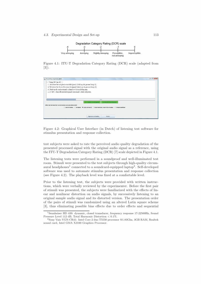
4.3. Experimental Design and Set-up 113
Figure 4.1: ITU-T Degradation Category Rating (DCR) scale (adapted from[3]).
Figure 4.2: Graphical User Interface (in Dutch) of listening test software forstimulus presentation and response collection.
test subjects were asked to rate the perceived audio quality degradation of thepresented processed signal with the original audio signal as a reference, usingthe ITU-T Degradation Category Rating (DCR) [7] scale depicted in Figure 4.1.
The listening tests were performed in a soundproof and well-illuminated testroom. Stimuli were presented to the test subjects through high-quality circum-aural headphones1 connected to a soundcard-equipped laptop2. Self-developedsoftware was used to automate stimulus presentation and response collection(see Figure 4.2). The playback level was fixed at a comfortable level.
Prior to the listening test, the subjects were provided with written instruc-tions, which were verbally reviewed by the experimenter. Before the first pairof stimuli was presented, the subjects were familiarized with the effects of lin-ear and nonlinear distortion on audio signals, by successively listening to anoriginal sample audio signal and its distorted version. The presentation orderof the pairs of stimuli was randomized using an altered Latin square scheme[3], thus eliminating possible bias effects due to order effects and sequential
1Sennheiser HD 439: dynamic, closed transducer, frequency response 17-22500Hz, SoundPressure Level 112 dB, Total Harmonic Distortion < 0.1%.
2Sony Vaio VGN-CR41: Intel Core 2 duo T5550 processor @1.83Ghz, 3GB RAM, Realteksound card, Intel GMA X3100 Graphics Processor.

114 Chapter 4. Subjective Audio Quality Evaluation
dependencies.
Imperceptible Perceptible Slightly Annoying Very annoying0
0.1
0.2
0.3
0.4
0.5
0.6
Degradation Category Rating
Rela
tive fre
quency
but notannoying
annoying
(a) Hard clipping, ODG=-1,“perceptible, but not annoying”.
Imperceptible Perceptible Slightly Annoying Very annoying0
0.1
0.2
0.3
0.4
0.5
0.6
Degradation Category Rating
Rela
tive fre
quency
but notannoying
annoying
(b) Perception-based clipping, ODG=-1,“perceptible, but not annoying”.
Imperceptible Perceptible Slightly Annoying Very annoying0
0.1
0.2
0.3
0.4
0.5
0.6
Degradation Category Rating
Rela
tive fre
quency
but notannoying
annoying
(c) Hard clipping, ODG=-2,“slightly annoying”.
Imperceptible Perceptible Slightly Annoying Very annoying0
0.1
0.2
0.3
0.4
0.5
0.6
Degradation Category RatingR
ela
tive fre
quency
but notannoying
annoying
(d) Perception-based clipping, ODG=-2,“slightly annoying”.
Imperceptible Perceptible Slightly Annoying Very annoying0
0.1
0.2
0.3
0.4
0.5
0.6
Degradation Category Rating
Rela
tive fre
quency
but notannoying
annoying
(e) Hard clipping, ODG=-3,“annoying”.
Imperceptible Perceptible Slightly Annoying Very annoying0
0.1
0.2
0.3
0.4
0.5
0.6
Degradation Category Rating
Rela
tive fre
quency
but notannoying
annoying
(f) Perception-based clipping, ODG=-3,“annoying”.
Figure 4.3: Histograms of DCR responses for the hard clipping algorithm (left)and the perception-based algorithm (right), for different hard clipped inputODGs.
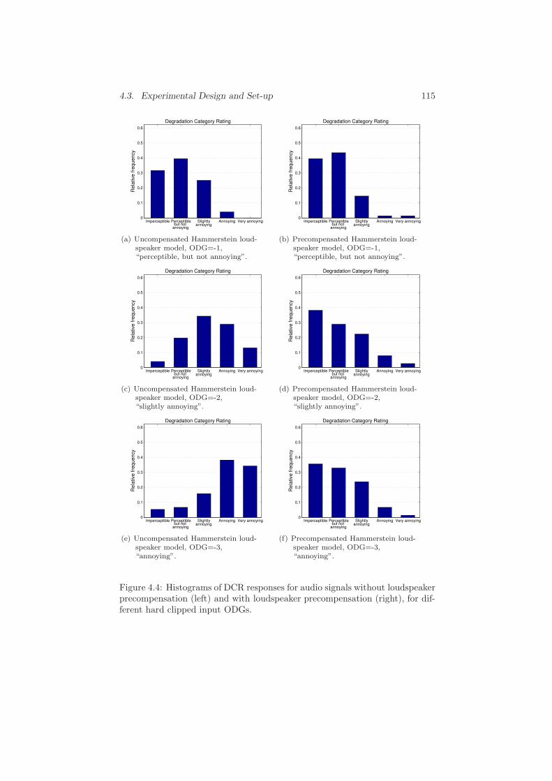
4.3. Experimental Design and Set-up 115
Imperceptible Perceptible Slightly Annoying Very annoying0
0.1
0.2
0.3
0.4
0.5
0.6
Degradation Category Rating
Rela
tive fre
quency
but notannoying
annoying
(a) Uncompensated Hammerstein loud-speaker model, ODG=-1,“perceptible, but not annoying”.
Imperceptible Perceptible Slightly Annoying Very annoying0
0.1
0.2
0.3
0.4
0.5
0.6
Degradation Category Rating
Rela
tive fre
quency
but notannoying
annoying
(b) Precompensated Hammerstein loud-speaker model, ODG=-1,“perceptible, but not annoying”.
Imperceptible Perceptible Slightly Annoying Very annoying0
0.1
0.2
0.3
0.4
0.5
0.6
Degradation Category Rating
Rela
tive fre
quency
but notannoying
annoying
(c) Uncompensated Hammerstein loud-speaker model, ODG=-2,“slightly annoying”.
Imperceptible Perceptible Slightly Annoying Very annoying0
0.1
0.2
0.3
0.4
0.5
0.6
Rela
tive fre
quency
Degradation Category Rating
but notannoying
annoying
(d) Precompensated Hammerstein loud-speaker model, ODG=-2,“slightly annoying”.
Imperceptible Perceptible Slightly Annoying Very annoying0
0.1
0.2
0.3
0.4
0.5
0.6
Degradation Category Rating
Rela
tive fre
quency
but notannoying
annoying
(e) Uncompensated Hammerstein loud-speaker model, ODG=-3,“annoying”.
Imperceptible Perceptible Slightly Annoying Very annoying0
0.1
0.2
0.3
0.4
0.5
0.6
Degradation Category Rating
Rela
tive fre
quency
but notannoying
annoying
(f) Precompensated Hammerstein loud-speaker model, ODG=-3,“annoying”.
Figure 4.4: Histograms of DCR responses for audio signals without loudspeakerprecompensation (left) and with loudspeaker precompensation (right), for dif-ferent hard clipped input ODGs.
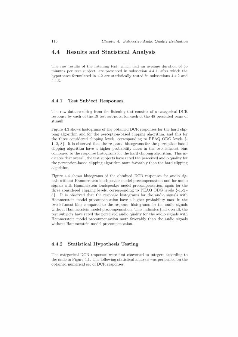
116 Chapter 4. Subjective Audio Quality Evaluation
4.4 Results and Statistical Analysis
The raw results of the listening test, which had an average duration of 35minutes per test subject, are presented in subsection 4.4.1, after which thehypotheses formulated in 4.2 are statistically tested in subsections 4.4.2 and4.4.3.
4.4.1 Test Subject Responses
The raw data resulting from the listening test consists of a categorical DCRresponse by each of the 19 test subjects, for each of the 48 presented pairs ofstimuli.
Figure 4.3 shows histograms of the obtained DCR responses for the hard clip-ping algorithm and for the perception-based clipping algorithm, and this forthe three considered clipping levels, corresponding to PEAQ ODG levels -1,-2,-3. It is observed that the response histograms for the perception-basedclipping algorithm have a higher probability mass in the two leftmost binscompared to the response histograms for the hard clipping algorithm. This in-dicates that overall, the test subjects have rated the perceived audio quality forthe perception-based clipping algorithm more favorably than the hard clippingalgorithm.
Figure 4.4 shows histograms of the obtained DCR responses for audio sig-nals without Hammerstein loudspeaker model precompensation and for audiosignals with Hammerstein loudspeaker model precompensation, again for thethree considered clipping levels, corresponding to PEAQ ODG levels -1,-2,-3. It is observed that the response histograms for the audio signals withHammerstein model precompensation have a higher probability mass in thetwo leftmost bins compared to the response histograms for the audio signalswithout Hammerstein model precompensation. This indicates that overall, thetest subjects have rated the perceived audio quality for the audio signals withHammerstein model precompensation more favorably than the audio signalswithout Hammerstein model precompensation.
4.4.2 Statistical Hypothesis Testing
The categorical DCR responses were first converted to integers according tothe scale in Figure 4.1. The following statistical analysis was performed on theobtained numerical set of DCR responses.
4.4. Results and Statistical Analysis 117
Testing Hypothesis 1
Let us denote the population DCR responses corresponding to audio signalsprocessed by the hard clipping algorithm and the perception-based clippingalgorithm by random variables RHC and RPBC, respectively.
Based on the sample DCR responses, we tested the following statistical hy-pothesis H1
0 against its alternative H1a :
H10 : RHC = RPBC (4.1)
H1a : RHC ≤ RPBC (4.2)
where R is the population median of the random variable R.
This statistical hypothesis was tested for all three considered ODGs using one-tailed Wilcoxon-Mann-Whitney tests [8] with significance level α = 0.05. Theresulting one-sided P-values are synthesized in the first column of Table 4.2.
From the obtained P-values, we conclude that the null hypothesis (4.1) can berejected in favor of the alternative (4.2) for all considered ODGs. The perceivedaudio quality of audio signals clipped by the perception-based clipping algo-rithm is not identical but significantly superior to that of audio signals clippedby the hard clipping algorithm, and this for all considered ODGs.
Testing Hypothesis 2
Let us denote the population DCR responses corresponding to audio signalsprocessed by the uncompensated Hammerstein loudspeaker model and the pre-compensated Hammerstein loudspeaker model by random variables RUNCOMP
and RCOMP, respectively.
Based on the sample DCR responses, we tested the following statistical hy-pothesis H2
0 against its alternative H2a :
H20 : RUNCOMP = RCOMP (4.3)
H2a : RUNCOMP ≤ RCOMP. (4.4)
This statistical hypothesis was tested for all three considered ODGs using one-tailed Wilcoxon-Mann-Whitney tests [8] with significance level α = 0.05. Theresulting one-sided P-values are synthesized in the second column of Table 4.2.
From the obtained P-values, we conclude that the null hypothesis (4.3) can berejected in favor of the alternative (4.4) for ODGs of -2 and -3. The perceivedaudio quality of audio signals processed by the proposed loudspeaker precom-pensation algorithm before being fed into the Hammerstein loudspeaker modelis not identical, but significantly superior to that of audio signals not pro-

118 Chapter 4. Subjective Audio Quality Evaluation
Table 4.2: P-values from one-tailed Wilcoxon-Mann-Whitney tests on sampleDCR responses. Significant P-values with respect to α = 0.05 in bold.
Null hypothesis → H10 H2
0 H30
ODG=-1 0.0006 0.0616 0.5062ODG=-2 <0.0001 <0.0001 0.4398ODG=-3 <0.0001 <0.0001 0.3374
cessed before being fed into the Hammerstein loudspeaker model, and this formoderate to high amplitude levels.
Testing Hypothesis 3
Based on the sample DCR responses, we tested the following statistical hy-pothesis H3
0 against its alternative H3a :
H30 : RUNCOMP = RHC (4.5)
H3a : RUNCOMP ≤ RHC. (4.6)
This statistical hypothesis was tested for all three considered ODGs using one-tailed Wilcoxon-Mann-Whitney tests [8] with significance level α = 0.05. Theresulting one-sided P-values are synthesized in the third column of Table 4.2.
From the obtained P-values, we conclude that the null hypothesis (4.5) cannotbe rejected in favor of the alternative (4.6) for any ODG. This means thatthere is no reason to believe that the perceived audio quality of audio signalssubject to a certain nonlinear hard clipping distortion would be superior to thatof audio signals subject to a combination of the same nonlinear hard clippingdistortion and an additional linear distortion.
4.4.3 Correlation Between Subjective and Objective Scores
As mentioned in Section 4.1, the PEAQ ODG measure has been designed toobjectively assess the perceptibility of degradations commonly encountered inaudio codecs. However, the nature of signal distortions introduced by clip-ping algorithms and (un)compensated Hammerstein loudspeaker models can berather different as compared to signal distortions introduced by audio codecs.Therefore, we will investigate the validity of using PEAQ ODG as an objectiveaudio quality measure in these alternative scenarios.
The correlation between subjective and objective scores is the most obviouscriterion to validate an objective method. Let us denominate the mean DCR

4.5. Conclusions 119
responses over all 19 test subjects as MDCR responses. Then we can calculatethe sample Pearson correlation coefficient ρ between the subjective MDCRresponses and the objective ODG scores as follows,
ρ =
∑Nps
i=1(MDCRi −MDCR)(ODGi −ODG)√∑Nps
i=1(MDCRi −MDCR)2√∑Nps
i=1(ODGi −ODG)2(4.7)
where
MDCR =
Nps∑
i=1
MDCRi (4.8)
and
ODG =
Nps∑
i=1
ODGi. (4.9)
Testing Hypothesis 4
The scatter plot of the mean subjective DCR scores against the objective ODGscores is shown in Figure 4.5. Based on the resulting sample Pearson correlationcoefficient value ρ = 0.67, we tested the following statistical hypothesis H4
0
against its alternative H4a :
H40 : ρ = 0 (4.10)
H4a : ρ > 0. (4.11)
where ρ is the population Pearson correlation coefficient.
This statistical hypothesis was tested [9] with significance level α = 0.05 byusing a one-tailed t-test having Nps− 2 degrees of freedom for the test statistic
value t = |ρ|√
Nps−2√1−ρ2
.
The resulting one-sided P-value is 1.206 · 10−7 < α, which means that the nullhypothesis (4.10) can be confidently rejected in favor of the alternative (4.11).In conclusion, there is a significant positive correlation between subjective audioquality scores and objective PEAQODG scores, supporting the validity of usingPEAQ ODG as an objective audio quality measure for audio signals processedby clipping algorithms and (un)compensated Hammerstein loudspeaker models.
4.5 Conclusions
Because of the limited applicability and accuracy of objective audio qualitymeasures, a formal subjective listening test has been performed in order to as-
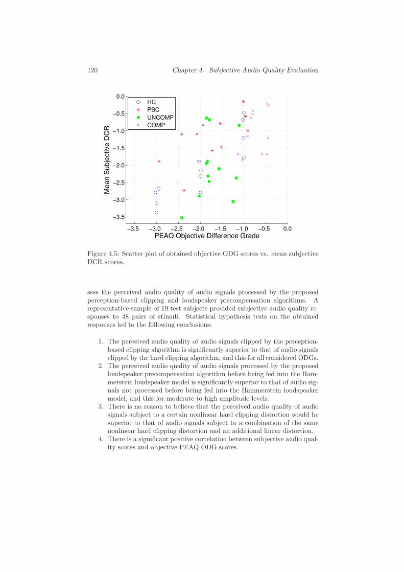
120 Chapter 4. Subjective Audio Quality Evaluation
−3.5 −3.0 −2.5 −2.0 −1.5 −1.0 −0.5 0.0
−3.5
−3.0
−2.5
−2.0
−1.5
−1.0
−0.5
0.0
PEAQ Objective Difference Grade
Mean S
ubje
ctive D
CR
HC
PBC
UNCOMP
COMP
Figure 4.5: Scatter plot of obtained objective ODG scores vs. mean subjectiveDCR scores.
sess the perceived audio quality of audio signals processed by the proposedperception-based clipping and loudspeaker precompensation algorithms. Arepresentative sample of 19 test subjects provided subjective audio quality re-sponses to 48 pairs of stimuli. Statistical hypothesis tests on the obtainedresponses led to the following conclusions:
1. The perceived audio quality of audio signals clipped by the perception-based clipping algorithm is significantly superior to that of audio signalsclipped by the hard clipping algorithm, and this for all considered ODGs.
2. The perceived audio quality of audio signals processed by the proposedloudspeaker precompensation algorithm before being fed into the Ham-merstein loudspeaker model is significantly superior to that of audio sig-nals not processed before being fed into the Hammerstein loudspeakermodel, and this for moderate to high amplitude levels.
3. There is no reason to believe that the perceived audio quality of audiosignals subject to a certain nonlinear hard clipping distortion would besuperior to that of audio signals subject to a combination of the samenonlinear hard clipping distortion and an additional linear distortion.
4. There is a significant positive correlation between subjective audio qual-ity scores and objective PEAQ ODG scores.

BIBLIOGRAPHY 121
Bibliography
[1] International Telecommunications Union Recommendation BS.1387,“Method for objective measurements of perceived audio quality,” 1998.
[2] C.-T. Tan, B. C. J. Moore, N. Zacharov, and V.-V. Mattila, “Predictingthe perceived quality of nonlinearly distorted music and speech signals,” J.Audio Eng. Soc., vol. 52, no. 7–8, pp. 699–711, Jul. 2004.
[3] S. Bech and N. Zacharov, Perceptual audio evaluation-Theory, method andapplication. Wiley, 2007.
[4] Red Hot Chili Peppers, “Californication,” Californication, Warner Bros.Records 9362473862, 1999.
[5] F. Chopin, “Waltz op. 69 no. 2,” Favourite Piano Works (Vladimir Ashke-nazy), Decca 02894448302, 1995.
[6] F. Poulenc, “Sonata for flute and piano (Cantilena),” French Flute Music,Naxos 8.557328, 2005.
[7] International Telecommunications Union Recommendation P. 800, “Meth-ods for subjective determination of transmission quality,” 1996.
[8] F. Wilcoxon, “Individual comparisons by ranking methods,” Biometricsbulletin, vol. 1, no. 6, pp. 80–83, 1945.
[9] S. Siegel, Nonparametric statistics for the behavioral sciences. McGraw-Hill, 1956.

122 Bibliography

Chapter 5
Embedded Hardware
Implementation
5.1 Introduction
This chapter considers the embedded hardware implementation on a field-programmable gate array (FPGA) of the core of the perception-based clippingalgorithm presented in Chapter 2. As the clipping algorithm is intended forreal-time audio signal processing on a typically small and portable device, thehardware design should preferably have a low latency, low power consumption,and low resource usage, while at the same time preserving a maximal audioquality.
The core of the perception-based clipping algorithm is formed by the solu-tion of a per-frame convex optimization problem. This clearly represents themost computationally intensive part of the perception-based clipping algorithm,hence our focus to restrict the hardware implentation to the optimization prob-lem solution method. The iterative optimal projected gradient method pro-posed in subsection 2.3.4 has several properties making it eligible for an effi-cient hardware implementation. Firstly, polynomial upper and lower boundshave been derived on the number of necessary iterations of the method to en-sure a given solution accuracy. This allows to choose a priori a fixed numberof iterations to ensure the desired solution accuracy, and at the same time al-lows to leave out a convergence test at every iteration. Secondly, the methoddoes not require the solution of a linear system of equations at every itera-
The work presented in this chapter was carried out in close cooperation with Dr. AndreaSuardi, Department of Electrical and Electronic Engineering, Imperial College, London, UK.
123
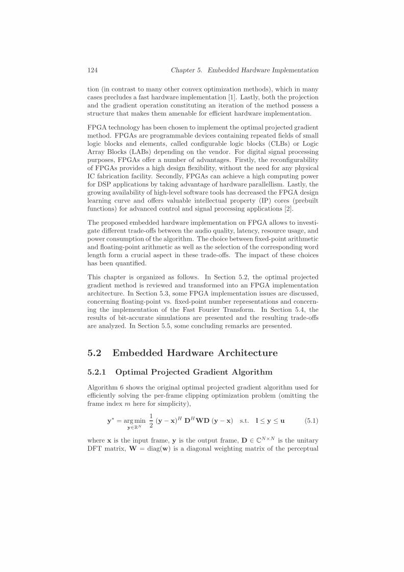
124 Chapter 5. Embedded Hardware Implementation
tion (in contrast to many other convex optimization methods), which in manycases precludes a fast hardware implementation [1]. Lastly, both the projectionand the gradient operation constituting an iteration of the method possess astructure that makes them amenable for efficient hardware implementation.
FPGA technology has been chosen to implement the optimal projected gradientmethod. FPGAs are programmable devices containing repeated fields of smalllogic blocks and elements, called configurable logic blocks (CLBs) or LogicArray Blocks (LABs) depending on the vendor. For digital signal processingpurposes, FPGAs offer a number of advantages. Firstly, the reconfigurabilityof FPGAs provides a high design flexibility, without the need for any physicalIC fabrication facility. Secondly, FPGAs can achieve a high computing powerfor DSP applications by taking advantage of hardware parallellism. Lastly, thegrowing availability of high-level software tools has decreased the FPGA designlearning curve and offers valuable intellectual property (IP) cores (prebuiltfunctions) for advanced control and signal processing applications [2].
The proposed embedded hardware implementation on FPGA allows to investi-gate different trade-offs between the audio quality, latency, resource usage, andpower consumption of the algorithm. The choice between fixed-point arithmeticand floating-point arithmetic as well as the selection of the corresponding wordlength form a crucial aspect in these trade-offs. The impact of these choiceshas been quantified.
This chapter is organized as follows. In Section 5.2, the optimal projectedgradient method is reviewed and transformed into an FPGA implementationarchitecture. In Section 5.3, some FPGA implementation issues are discussed,concerning floating-point vs. fixed-point number representations and concern-ing the implementation of the Fast Fourier Transform. In Section 5.4, theresults of bit-accurate simulations are presented and the resulting trade-offsare analyzed. In Section 5.5, some concluding remarks are presented.
5.2 Embedded Hardware Architecture
5.2.1 Optimal Projected Gradient Algorithm
Algorithm 6 shows the original optimal projected gradient algorithm used forefficiently solving the per-frame clipping optimization problem (omitting theframe index m here for simplicity),
y∗ = argminy∈RN
1
2(y − x)H DHWD (y − x) s.t. l ≤ y ≤ u (5.1)
where x is the input frame, y is the output frame, D ∈ CN×N is the unitaryDFT matrix, W = diag(w) is a diagonal weighting matrix of the perceptual

5.2. Embedded Hardware Architecture 125
Memory 2
(y_o)
Memory 1
(c_o)
Memory 3
(gradient_o)
clip_iter
clip_pipe
Memory 2
(y_i)
Memory 1
(c_i)
Memory 3
(gradient_i) scaling
C 1 U L x w
clip_top
y*
Kmax
clip_weight
Figure 5.1: Block diagram representing the implementation of the clippingoptimal projected gradient algorithm onto FPGA.
weights w, and u = U1N and l = L1N contain the upper and lower clippinglevels.
In order to allow for an efficient hardware implementation, we have performedthe following organizational changes in Algorithm 6 without altering its func-tionality, as shown in the adapted Algorithm 7:
1. Several algorithm parameters need not be computed on-line, but canrather be precomputed off-line:
• The per-iteration weights δk are precomputed off-line, using lines 2-3-4-10-11 of Algorithm 6. The resulting precomputed weight vectorδ = [δ0, δ1, . . . , δKmax−1]T is defined as an input to the adaptedAlgorithm 7.
• The Lipschitz constant C is precomputed off-line, and the inverseof the Lipschitz constant C−1 is defined as an input to the adaptedAlgorithm 7. This way, the division operation by C on line 8 ofAlgorithm 6, is replaced by a more hardware-friendly multiplicationwith C−1 on line 5 of the adapted Algorithm 7.
2. The computation of the gradient was rescheduled from the start of theiteration (line 7 in Algorithm 6) to the end of the iteration (line 8 inAlgorithm 7), thus reducing the overall algorithm delay.
5.2.2 FPGA Implementation Architecture
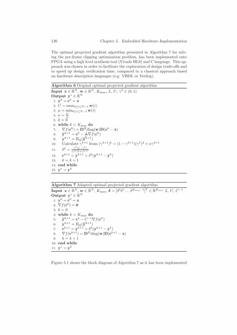
126 Chapter 5. Embedded Hardware Implementation
The optimal projected gradient algorithm presented in Algorithm 7 for solv-ing the per-frame clipping optimization problem, has been implemented ontoFPGA using a high level synthesis tool (Vivado HLS) and C language. This ap-proach was chosen in order to facilitate the exploration of design trade-offs andto speed up design verification time, compared to a classical approach basedon hardware description languages (e.g. VHDL or Verilog).
Algorithm 6 Original optimal projected gradient algorithm
Input x ∈ RN , w ∈ RN , Kmax, L, U , γ0 ∈ (0, 1)Output y∗ ∈ RN
1: y0 = c0 = x2: C = max0≤i≤N−1 w(i)3: µ = min0≤i≤N−1 w(i)4: κ = C
µ
5: k = 06: while k < Kmax do7: ∇f(ck) = DHdiag(w)D(ck − x)8: yk+1 = ck − 1
C∇f(ck)
9: yk+1 = ΠQ(yk+1)
10: Calculate γk+1 from (γk+1)2 = (1− γk+1)(γk)2 + κγk+1
11: δk = γk(1−γk)(γk)2+γk+1
12: ck+1 = yk+1 + δk(yk+1 − yk)13: k = k + 114: end while15: y∗ = yk
Algorithm 7 Adapted optimal projected gradient algorithm
Input x ∈ RN , w ∈ RN , Kmax, δ = [δ0δ1 . . . δKmax−1]T ∈ RKmax L, U , C−1
Output y∗ ∈ RN
1: y0 = c0 = x2: ∇f(c0) = 03: k = 04: while k < Kmax do5: yk+1 = ck − C−1∇f(ck)6: yk+1 = ΠQ(y
k+1)7: ck+1 = yk+1 + δk(yk+1 − yk)8: ∇f(ck+1) = DHdiag(w)D(ck+1 − x)9: k = k + 1
10: end while11: y∗ = yk
Figure 5.1 shows the block diagram of Algorithm 7 as it has been implemented

5.3. FPGA Implementation Aspects 127
onto FPGA, where each module has been coded using a specific C function.The main function clip top consists of an iterative implementation of theper-iteration function clip iter. In every iteration, the variables ck+1, yk+1
and ∇f(ck+1) are stored in the respective memory blocks Memory 1, Memory2 and Memory 3, in order to be accessed in the next iteration. The per-iteration function clip iter consists of the following five subfunctions (thecorresponding lines in Algorithm 2 are given in brackets):
• clip pipe (lines 5-7) implements the gradient step, the projection ontothe feasible set, and the computation of the weighted sum of previousiterates. It involves a sequence of element-by-element operations, thatcan be pipelined to reduce overall delay.
• FFT (line 8) implements the Fast Fourier Transform (FFT), for which theconfiguration parameters are set up in the function config fft. Detailson the FFT function an its configuration are given in subsection 5.3.2.
• clip weight (line 8) implements the point-wise multiplication of theFFT output with the perceptual weights.
• IFFT (line 8) implements the inverse Fast Fourier Transform (IFFT), forwhich the configuration parameters are set up in the function config ifft.Details on the IFFT function an its configuration are given in subsection5.3.2.
• clip scale performs a descaling of the IFFT output.
5.3 FPGA Implementation Aspects
5.3.1 Floating-Point and Fixed-Point Arithmetic
FPGAs allow for a variety of computer arithmetic implementations, as theysupport both floating-point and fixed-point arithmetic. We will review herethe main properties of floating-point and fixed-point arithmetic, and point outthe pros and cons of using these arithmetics.
Floating-Point Arithmetic
The most commonly used floating point formats are described by the IEEE754 standard [3]. As shown in Figure 5.2(a), the single-precision floating-pointrepresentation adopts a 32-bit architecture which uses 1 bit for the sign, 23bits for the fractional part of the mantissa, and 8 bits for the signed exponentvalue, which moves the binary radix point with respect to the mantissa. Thefollowing relation holds between the single-precision floating-point value Vfloatand its corresponding bit representation:
Vfloat = (−1)s0︸ ︷︷ ︸
sign
M︸︷︷︸
mantissa
2E−127︸ ︷︷ ︸
exponential
(5.2)

128 Chapter 5. Embedded Hardware Implementation
(a) Floating point
(b) Fixed point
Figure 5.2: Floating and fixed point number representations.
where the mantissa M consists of a fixed integer part and a variable fractionalpart,
M = 1︸︷︷︸
integer
+
23∑
i=1
b23−i2−i
︸ ︷︷ ︸
fractional
(5.3)
and the decimal exponent E is
E =
7∑
i=0
ei2i. (5.4)
The most advantageous property of floating point arithmetic is that the ex-ponent of each value can be selected to allow for maximum precision, and theexponent is stored with the fractional data. This allows to represent a widerange of numbers with a relatively small number of bits.
The main disadvantage is the need for additional hardware and longer delaysfor performing denormalization and normalization of the operands before andafter every addition and subtraction [4] [5].

5.3. FPGA Implementation Aspects 129
Fixed-Point Arithmetic
Fixed-point numbers use a fixed number of bits for the integer and the fractionalparts. The exponent does not vary and does not have to be stored. The fixed-point example shown in Figure 5.2(b) adopts a 32-bit architecture, which uses 1bit for the sign, 27 bits for the fractional part, and 4 bits for the integer part. Inreality, an adder or any other arithmetic circuit does not know how many bitsare interpreted as integer or fractional. This is purely an interpretational issue,so one can practically think of fixed-point arithmetic as integer arithmetic [6].
The following relation holds between the fixed-point value Vfix and its corre-sponding bit representation:
Vfix =
30∑
i=0
bi2i−27
︸ ︷︷ ︸
integer+fractional
−s024︸ ︷︷ ︸
2’s complement
(5.5)
where the 2’s complement format is generally used because it allows to performsubtraction and addition with the same hardware architecture.
The main advantage of using fixed-point implementations is the resulting lowercost and lower power, and often higher speed compared to floating-point im-plementations [2]. On FPGA platforms, there is the additional advantage ofthe fixed-point implementation being easily customizable to almost any desiredword length [4].
The main disadvantage related to fixed-point implementations is the lower dy-namic range and reduced precision compared to floating-point, which leadsto different types of errors that can be incurred when performing fixed-pointcomputations [1]:
• Quantization errors : these errors are introduced when high-precision in-put data is converted to the adopted reduced-precision fixed-point dataformat.
• Overflow errors : these errors are introduced whenever the number ofbits for the integer part in the fixed-point representation is too small torepresent a given number, e.g. after adding two numbers of like sign.In our proposed FPGA implementation, the number of integer bits wasconservatively chosen large enough (5 bits) in order to avoid overflow.
• Arithmetic errors : these errors are introduced when multiplying twonumbers having b fraction bits. The exact product can be representedusing 2b fraction bits, so a b-bit truncation of the 2’s complement numberis necessary and introduces a round-off error.
Amongst the possible consequences of these errors occurring in the fixed-pointimplementation of an optimization method, are the loss of problem convexity,
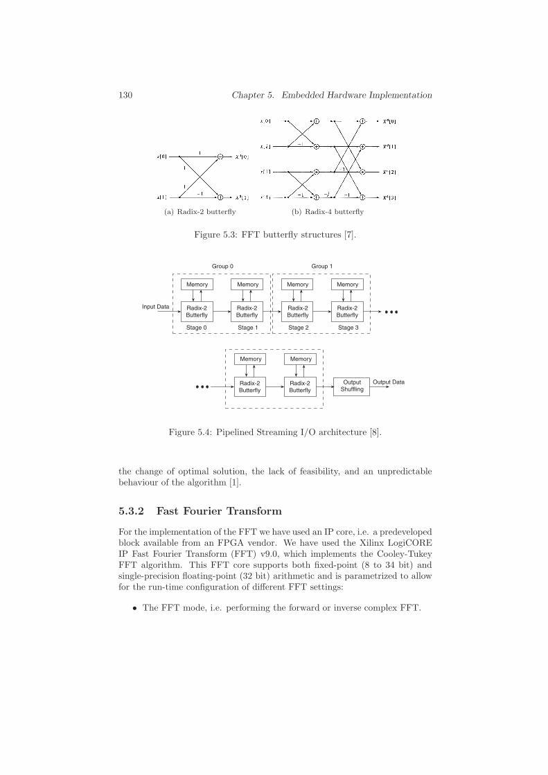
130 Chapter 5. Embedded Hardware Implementation
(a) Radix-2 butterfly (b) Radix-4 butterfly
Figure 5.3: FFT butterfly structures [7].
Memory
Memory Memory
Memory Memory Memory
Radix-2Butterfly
Radix-2Butterfly
Radix-2Butterfly
Radix-2Butterfly
Radix-2Butterfly
Radix-2Butterfly
Group 0 Group 1
Stage 0 Stage 1 Stage 2 Stage 3
OutputShuffling
Output Data
Input Data
Figure 5.4: Pipelined Streaming I/O architecture [8].
the change of optimal solution, the lack of feasibility, and an unpredictablebehaviour of the algorithm [1].
5.3.2 Fast Fourier Transform
For the implementation of the FFT we have used an IP core, i.e. a predevelopedblock available from an FPGA vendor. We have used the Xilinx LogiCOREIP Fast Fourier Transform (FFT) v9.0, which implements the Cooley-TukeyFFT algorithm. This FFT core supports both fixed-point (8 to 34 bit) andsingle-precision floating-point (32 bit) arithmetic and is parametrized to allowfor the run-time configuration of different FFT settings:
• The FFT mode, i.e. performing the forward or inverse complex FFT.

5.3. FPGA Implementation Aspects 131
Figure 5.5: Resource usage versus throughput for FFT architecture options [8].
• The FFT transform size N = 2m, m = 3− 16.• The scaling schedule, which represents the number of bits to be shifted
after each stage of the FFT to avoid overflow, e.g. a scaling schedule of[2 3 2 0 1] bit-shifts (ordered from the first to the last stage) could beused for a five-stage implementation.
The FFT core provides four architecture options to trade-off resource usageand transform time. The basic blocks of all four FFT architectures are theso-called FFT Radix-r butterflies, which take in r complex data values andprocess them to produce a new set of r complex data values [9]. Figure 5.3(a)and Figure 5.3(b) show the structure of such a Radix-2 butterfly and a Radix-4butterfly, respectively. The four resulting FFT architectures are the following:
• Pipelined Streaming I/O: from Figure 5.4, we observe that log2N Radix-2 butterfly processing stages are pipelined to offer continuous data pro-cessing. Each processing stage has its own memory banks to store inputand intermediate data. The core has the ability to simultaneously per-form transform calculations on the current frame of data, load input datafor the next frame of data, and unload the results of the previous frameof data. The data is scaled after every pair of Radix-2 stages.
• Radix-4 Burst I/O: loads and processes data separately. The N -pointFFT consists of log4N stages, with each stage containing N
4 Radix-4butterflies. Transform sizes that are not a power of 4 need an extraRadix-2 stage for combining data.
• Radix-2 Burst I/O: loads and processes data separately. The N -pointFFT consists of log2N stages, with each stage containing N
2 Radix-2butterflies.
• Radix-2 Lite Burst I/O: a variant of Radix-2 Burst I/O with reduced

132 Chapter 5. Embedded Hardware Implementation
clip_top
U
L
load tests
data
from files
write results
data
to file
clip_tb.cpp
write tests
files
read results
files
write_testbench.m read_testbench.mclip.cpp
C 1
w
Kmax
y*
x
Figure 5.6: Data flow for the bit-accurate FPGA simulation in Vivado HLS.
resource usage at the expense of an additional delay.
The trade-off between resource usage and transform time for the different FFTarchitectures is illustrated in Figure 5.5. In order to minimize the transformtime, we have selected to use the Pipelined Streaming I/O architecture, yet thischoice comes with the cost of a higher resource usage. The following parametershave been selected:
• Transform size N = 512 = 29.• Fixed conservative scaling schedule of [2 2 2 2 1] bit-shifts for the different
FFT stages, which completely avoids overflows.
5.4 Simulation Results
5.4.1 Simulation Set-up
The C implementation of the architecture shown in Figure 5.1 has been trans-formed using Vivado HLS into a Register Transfer Level (RTL) implementation,which can be directly synthesized into any Xilinx FPGA.
In order to perform bit-accurate simulations of the RTL implementation, a sim-ulation framework connecting Vivado HLS and MATLAB has been created, asshown in Figure 5.6. The input test data are stored into files using MATLAB(write testbench.m), then read by the Vivado HLS bit-accurate simulationengine (clip tb.cpp), and finally the simulation results are loaded into MAT-LAB (read testbench.m). The simulation framework supports floating-pointsingle-precision arithmetic and any fixed-point arithmetic up to 34 bits.
Two audio signals, chopin.wav and mascagni.wav, were selected to generatethe input test data. The input test data per audio signal consists of all audiosignal frames (N = 512) in which at least one sample exceeds a given amplitude

5.4. Simulation Results 133
range [L,U ], where the symmetric clipping level U = −L was fixed at 0.14 and0.25 for the respective audio signals. This procedure resulted in 86 and 233audio signal frames constituting the input test data, respectively.
The RTL synthesis and bit-accurate simulations were performed for differentsettings of the applied arithmetic:
• Floating-point single-precision arithmetic (32 bits)• Fixed-point arithmetic using b =12,14,16,18,20,22,24,26,28,30,32,34 frac-
tion bits.
For every considered arithmetic setting, the bit-accurate simulations were re-peated for different values of the fixed number of iterationsKmax=10,20,30,40,50of the optimal projected gradient method.
5.4.2 Accuracy in Fixed-Point Arithmetic
We have computed the mean-squared error (MSE) between the output audiosignal frame y∗ computed using bit-accurate hardware simulations in fixed-point or single-precision floating point arithmetic, and the reference output au-dio signal frame y∗ computed using double-precision floating-point arithmeticin MATLAB,
MSE(y∗) =1
N
N∑
i=1
(y∗i − y∗i )2 (5.6)
In Figures 5.7(a) and 5.7(b), the MSE for all audio signal frames is plottedfor the different fixed-point and floating-point arithmetics, for Kmax = 50. Forboth audio signals, we observe a fairly constant MSE over all audio signal framesfor a given arithmetic choice. The per-frame MSE in fixed-point arithmetic isseen to improve by roughly a decade per two additional fraction bits. Whenusing the maximum of 34 fixed-point fraction bits, the MSE values approachthe MSE in single-precision floating point, which is as low as 10−14.
The MSE gives an indication of the per-frame accuracy, which is not sufficientto draw conclusions on the quality of the complete audio signal. In order toassess which is the minimum number of fixed-point fraction bits to be usedfrom an audio quality point of view, the following analysis has been conducted.
The objective audio quality difference for each audio signal is assessed by com-puting the ∆ODG measure,
∆ODG = ODG(xs,y∗s )−ODG(xs, y
∗s ) (5.7)
where xs is the input audio signal, y∗s is the reference output audio signal
computed using double-precision floating-point arithmetic in Matlab, and y∗s

134 Chapter 5. Embedded Hardware Implementation
Kmax — b 12 16 20 24 28 32 3410 0.803 0.245 0.070 0.045 0.046 0.046 0.04620 0.804 0.549 0.036 0.025 0.023 0.023 0.02330 0.797 0.417 0.011 0.011 0.009 0.009 0.00940 0.793 0.466 0.022 0.001 0.003 0.003 0.00250 0.786 0.497 0.042 0.002 0.000 0.000 0.000
Table 5.1: ∆ODG audio quality difference with respect to double precisionimplementation, with b the number of fixed-point fraction bits employed andKmax the fixed number of iterations, for fragment chopin.wav. Imperceptibledifferences in bold.
Kmax — b 12 16 20 24 28 32 3410 0.254 0.120 0.058 0.049 0.049 0.049 0.04920 0.254 0.057 0.027 0.021 0.021 0.021 0.02130 0.255 0.099 0.006 0.006 0.006 0.006 0.00640 0.254 0.121 0.004 0.001 0.001 0.000 0.00050 0.254 0.135 0.012 0.001 0.000 0.000 0.000
Table 5.2: ∆ODG audio quality difference with respect to double precisionimplementation, with b the number of fixed-point fraction bits employed andKmax the fixed number of iterations, for fragment mascagni.wav. Impercepti-ble differences in bold.
is the output audio signal computed using bit-accurate hardware simulationsin fixed-point or single-precision floating point arithmetic. ODG(r,d) is an ob-jective measure [10] which predicts the audio quality of a signal d with respectto a signal r on a scale of [0,−4], where 0 corresponds to an imperceptibledegradation, and -4 corresponds to a very annoying degradation.
In Tables 5.1 and 5.2, the ∆ODG audio quality difference is given for differentvalues of the number of fixed-point fraction bits b and the number of itera-tions Kmax. An interesting observation is that in some cases, the audio qualitydifference increases with the number of iterations due to the increasing accumu-lation of round-off errors. As the resolution of the ODG is 0.02 points [10], wecan interpret differences falling within 0.02 ODG points as being imperceptible(boldfaced values). For both audio signals, it is seen to be sufficient to performKmax = 30 projected gradient iterations using b = 20 fixed-point fraction bitsin order to avoid perceptible artefacts.
5.4.3 Latency, Resource Usage and Power Consumption
Depending on the employed arithmetic, the FPGA design will exhibit differentcharacteristics in terms of overall latency, resource usage and power consump-tion. We have assessed these relations using Vivado HLS, selecting a Xilinx

5.4. Simulation Results 135
0 20 40 60 80 100 120
10−14
10−12
10−10
10−8
10−6
10−4
10−2
Frame number
MS
E
fix12
fix14
fix16
fix18
fix20
fix22
fix24
fix26
fix28
fix30
fix32
fix34
float32
(a) chopin.wav
0 50 100 150 200 250 300
10−14
10−12
10−10
10−8
10−6
10−4
10−2
Frame number
MS
E
fix12
fix14
fix16
fix18
fix20
fix22
fix24
fix26
fix28
fix30
fix32
fix34
float32
(b) mascagni.wav
Figure 5.7: MSE per audio signal frame for different fixed-point and floating-point arithmetics, Kmax = 50.
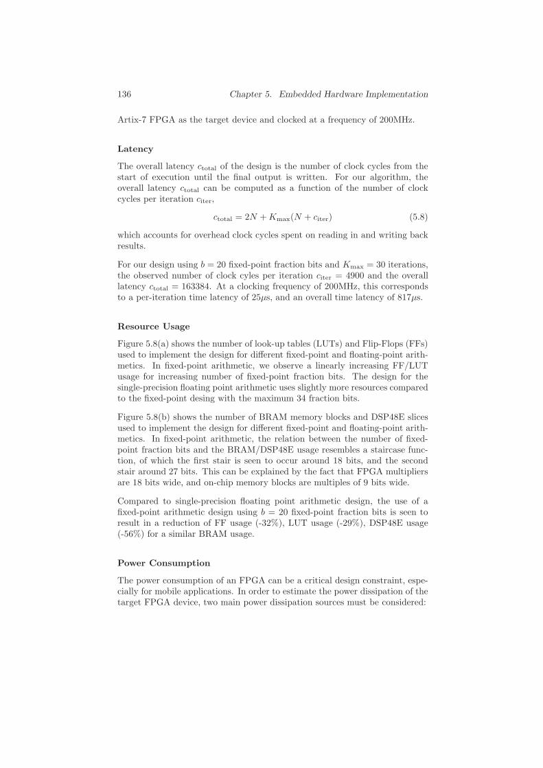
136 Chapter 5. Embedded Hardware Implementation
Artix-7 FPGA as the target device and clocked at a frequency of 200MHz.
Latency
The overall latency ctotal of the design is the number of clock cycles from thestart of execution until the final output is written. For our algorithm, theoverall latency ctotal can be computed as a function of the number of clockcycles per iteration citer,
ctotal = 2N +Kmax(N + citer) (5.8)
which accounts for overhead clock cycles spent on reading in and writing backresults.
For our design using b = 20 fixed-point fraction bits and Kmax = 30 iterations,the observed number of clock cyles per iteration citer = 4900 and the overalllatency ctotal = 163384. At a clocking frequency of 200MHz, this correspondsto a per-iteration time latency of 25µs, and an overall time latency of 817µs.
Resource Usage
Figure 5.8(a) shows the number of look-up tables (LUTs) and Flip-Flops (FFs)used to implement the design for different fixed-point and floating-point arith-metics. In fixed-point arithmetic, we observe a linearly increasing FF/LUTusage for increasing number of fixed-point fraction bits. The design for thesingle-precision floating point arithmetic uses slightly more resources comparedto the fixed-point desing with the maximum 34 fraction bits.
Figure 5.8(b) shows the number of BRAM memory blocks and DSP48E slicesused to implement the design for different fixed-point and floating-point arith-metics. In fixed-point arithmetic, the relation between the number of fixed-point fraction bits and the BRAM/DSP48E usage resembles a staircase func-tion, of which the first stair is seen to occur around 18 bits, and the secondstair around 27 bits. This can be explained by the fact that FPGA multipliersare 18 bits wide, and on-chip memory blocks are multiples of 9 bits wide.
Compared to single-precision floating point arithmetic design, the use of afixed-point arithmetic design using b = 20 fixed-point fraction bits is seen toresult in a reduction of FF usage (-32%), LUT usage (-29%), DSP48E usage(-56%) for a similar BRAM usage.
Power Consumption
The power consumption of an FPGA can be a critical design constraint, espe-cially for mobile applications. In order to estimate the power dissipation of thetarget FPGA device, two main power dissipation sources must be considered:
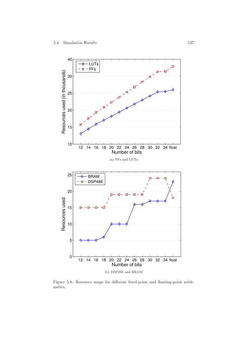
5.4. Simulation Results 137
12 14 16 18 20 22 24 26 28 30 32 34 float10
15
20
25
30
40
Number of bits
Re
so
urc
es u
se
d (
in t
ho
usa
nd
s)
LUTs
FFs
(a) FFs and LUTs
12 14 16 18 20 22 24 26 28 30 32 34 float0
5
10
15
20
25
Number of bits
Re
so
urc
es u
se
d
BRAM
DSP48E
(b) DSP48E and BRAM
Figure 5.8: Resource usage for different fixed-point and floating-point arith-metics.
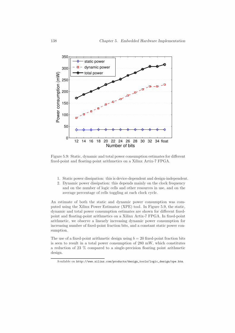
138 Chapter 5. Embedded Hardware Implementation
12 14 16 18 20 22 24 26 28 30 32 34 float0
50
100
150
200
250
300
350
Number of bits
Po
we
r co
nsu
mp
tio
n (
mW
)
static power
dynamic power
total power
Figure 5.9: Static, dynamic and total power consumption estimates for differentfixed-point and floating-point arithmetics on a Xilinx Artix-7 FPGA.
1. Static power dissipation: this is device-dependent and design-independent.2. Dynamic power dissipation: this depends mainly on the clock frequency
and on the number of logic cells and other resources in use, and on theaverage percentage of cells toggling at each clock cycle.
An estimate of both the static and dynamic power consumption was com-puted using the Xilinx Power Estimator (XPE) tool. In Figure 5.9, the static,dynamic and total power consumption estimates are shown for different fixed-point and floating-point arithmetics on a Xilinx Artix-7 FPGA. In fixed-pointarithmetic, we observe a linearly increasing dynamic power consumption forincreasing number of fixed-point fraction bits, and a constant static power con-sumption.
The use of a fixed-point arithmetic design using b = 20 fixed-point fraction bitsis seen to result in a total power consumption of 280 mW, which constitutesa reduction of 23 % compared to a single-precision floating point arithmeticdesign.
Available on http://www.xilinx.com/products/design_tools/logic_design/xpe.htm.

5.5. Conclusions 139
5.5 Conclusions
This chapter has considered an embedded hardware implementation on anFPGA of the optimal projected gradient method, which forms the core of theperception-based clipping algorithm. It was demonstrated that the choice be-tween fixed-point arithmetic and floating-point arithmetic and the selection ofthe corresponding bit width has an impact on the resulting audio quality aswell as on the resource usage and power consumption of the design.
The resulting FPGA design, which performs 30 projected gradient iterationsusing 20 fixed-point fraction bits, has a low latency, a reduced power consump-tion, a reduced resource usage, and at the same time preserves the full audioquality improvement. This design thus allows to perform the algorithm in realtime on a small and portable device.
Bibliography
[1] J. L. Jerez, P. J. Goulart, S. Richter, G. A. Constantinides, E. C. Kerrigan,and M. Morari, “Embedded online optimization for model predictive con-trol at megahertz rates,” Submitted to IEEE Transactions on AutomaticControl, 2013.
[2] U. Meyer-Baese, Digital Signal Processing with Field Programmable GateArrays. Springer, 2007.
[3] IEEE, “IEEE standard for binary floating-point arithmetic,” Std 754-1985,1985.
[4] W. T. Padgett and D. V. Anderson, “Fixed-point signal processing,” Syn-thesis Lectures on Signal Processing, vol. 4, no. 1, pp. 1–133, 2009.
[5] S. W. Smith et al., The scientist and engineer’s guide to digital signalprocessing. California Technical Pub. San Diego, 1997.
[6] J. Serrano, “Introduction to FPGA design,” in 8th Workshop on Electron-ics for LHC Experiments. CERN, 2004, pp. 231–247.
[7] B. Porat, A course in digital signal processing. Wiley New York, 1997.
[8] “LogiCORE IP Fast Fourier Transform v9.0 Product Guide for Vi-vado Design Suite,” http://www.xilinx.com/support/documentation/ipdocumentation/xfft/v9 0/pg109-xfft.pdf, accessed: 2013-10-21.
[9] P. Kabal and B. Sayar, “Performance of fixed-point FFT’s: Rounding andscaling considerations,” in IEEE International Conference on Acoustics,Speech, and Signal Processing, vol. 11, 1986, pp. 221–224.

140 Bibliography
[10] International Telecommunications Union Recommendation BS.1387,“Method for objective measurements of perceived audio quality,” 1998.

Part III
Recovery Algorithms

142

Chapter 6
Declipping Using
Perceptual Compressed
Sensing
Declipping of Audio Signals Using Perceptual
Compressed Sensing
Bruno Defraene, Naim Mansour, Steven De Hertogh,
Toon van Waterschoot, Moritz Diehl, and Marc Moonen
Published in IEEE Trans. Audio Speech Language Process., vol.21, no. 12, Dec. 2013, pp. 2627-2637.
c©2013 IEEE. Personal use of this material is permitted. Permission fromIEEE must be obtained for all other uses, including reprinting/republishingthis material for advertising or promotional purposes, creating new collectiveworks for resale or redistribution to servers or lists, or reuse of any copyrightedcomponent of this work in other works.
143

144 Chapter 6. Declipping Using Perceptual Compressed Sensing
Contributions of first author
• literature study• co-design of perceptual compressed sensing framework• co-development of PCSL1 declipping algorithm• co-design of objective evaluation experiments• software implementation and computer simulations• co-interpretation of objective evaluation results• co-design and supervision of subjective listening tests• co-analysis and co-interpretation of subjective evaluation re-
sults• co-formulation of conclusions• text redaction and editing
6.1. Introduction 145
Abstract
The restoration of clipped audio signals, commonly known as declipping, isimportant to achieve an improved level of audio quality in many audio appli-cations. In this paper, a novel declipping algorithm is presented, jointly basedon the theory of compressed sensing (CS) and on well-established propertiesof human auditory perception. Declipping is formulated as a sparse signal re-covery problem using the CS framework. By additionally exploiting knowledgeof human auditory perception, a novel perceptual compressed sensing (PCS)framework is devised. A PCS-based declipping algorithm is proposed whichuses ℓ1-norm type reconstruction. Comparative objective and subjective eval-uation experiments reveal a significant audio quality increase for the proposedPCS-based declipping algorithm compared to CS-based declipping algorithms.
6.1 Introduction
Clipping introduces undesired signal distortion in many audio applications.Clipping can occur both in the analog domain and in the digital domain, and isgenerally caused by the inability of an audio playback, recording or processingdevice to deliver the dynamic range required by the audio signal. When adigital audio signal is clipped, all its sample values lying beyond a maximumamplitude level (referred to as the clipping level θc) are mapped onto ±θc, asshown in Figure 6.1.
Clipping inevitably introduces nonlinear distortion into the audio signal, con-sisting of both the modification of existing frequency components, and the in-troduction of new harmonic and aliasing frequency components into the signal[1]. In a series of listening experiments [2], it has been concluded that clippinghas a significant negative effect on the perceived audio quality. More specifi-cally, clipping is typically associated with the perceptible addition of cracklingnoises to the original audio signal, often qualified as (very) annoying.
Therefore, performing declipping, i.e. the restoration of the clipped audio sig-nal, is necessary to achieve an improved level of audio quality and listenersatisfaction. In past research contributions, several approaches to the declip-ping problem have been proposed. A first approach is based on performing aninterpolation/extrapolation step to recover the clipped signal portions basedon the knowledge of unclipped signal portions [3]. A second approach consistsin adopting a suitable model of both the clean signal (typically autoregres-sive) and the clipping distortion, and subsequently recovering the clean signal
In the context of this research, digital hard clipping is considered, and it will be simplytermed “clipping” throughout this paper. Note that in analogue systems, soft clipping isvery common.

146 Chapter 6. Declipping Using Perceptual Compressed Sensing
Figure 6.1: Clipping of a digital audio signal.
through Bayesian statistical estimation of its model parameters [4]. Other no-table declipping approaches include the use of artificial neural networks [5].
Recently, the declipping problem has been adressed in the generic framework ofcompressed sensing (CS), and encouraging results have been reported [6, 7, 8, 9].In the CS framework, declipping is formulated and solved as a sparse signalrecovery problem, where one takes advantage of the sparsity of the clean audiosignal (in some basis) in order to recover it from a subset of its samples.
In this paper, we propose a perceptual compressed sensing (PCS) framework, inwhich a declipping algorithm is subsequently developed. The PCS frameworkintegrates CS theory and properties of human auditory perception. By incor-porating knowledge of human auditory perception in the algorithm design, it ispossible to further improve the perceptual reconstruction quality. The advan-tage of using perceptual knowledge has been recently demonstrated in relatedaudio applications, such as the sparse approximation of audio signals [10], andthe limiting of audio signals [11].
The paper is organized as follows. In Section 6.2, the basic principles of CS aswell as its fundamental limitations are reviewed, and the declipping problem issubsequently formulated in the CS framework. In Section 6.3, the PCS frame-work is presented, leading to a PCS-based declipping algorithm, using ℓ1-normtype reconstruction. In Section 6.4, a comparative objective and subjectiveevaluation of different declipping algorithms is discussed. Finally, in Section6.5, some concluding remarks are presented.
6.2 A CS Framework for Declipping
The theory of compressed sensing has been introduced in [12] [13] [14] in thecontext of sparse signal sampling and acquisition. Basically, the theory statesthat any signal that can be considered sparse in some basis, can be uniquely,and in many cases perfectly reconstructed based on sub-Nyquist rate sampled

6.2. A CS Framework for Declipping 147
measurements. This notion goes against the commonly accepted Nyquist sam-pling criterion. In the next subsections, we review the basic principles of CS aswell as its fundamental limitations, and subsequently formulate the declippingproblem in the CS framework.
6.2.1 CS Basic Principles
To be able to outline the basic principles of CS, we first introduce some neces-sary definitions and notation. Signals are considered to be real-valued vectorsin an N -dimensional normed Euclidean vector space RN . For the purposes ofCS, mainly the ℓ0 and ℓ1 norm are of importance. The sparsity k of a vectorx is defined as the number of non-zero components, i.e. ‖x‖0 = k. A vector xwith sparsity k is said to be k-sparse.
Compressed sensing takes advantage of the sparsity of a signal s ∈ RN in somefixed basis Ψ ∈ CN×N in order to recover it from a reduced measurementy ∈ RM , whereM < N . Acquiring a signal s by CS consists of two main steps:
1. Measurement : apply a measurement matrix Φ to obtain the measure-ment y,
y = Φs = ΦΨx = Ax (6.1)
with s ∈ RN the original signal, x ∈ R
N its sparse decomposition,Ψ ∈ CN×N the fixed basis, Φ ∈ RM×N the measurement matrix,A = ΦΨ ∈ CM×N the sensing matrix, and y ∈ RM the measurement.
2. Recovery: (in)exactly recover s′ from y using constrained ℓp-norm opti-mization,
x′ = argminz
‖z‖p subject to Az = y (6.2)
s′ = Ψx′ (6.3)
with p ∈ 0, 1 in typical CS applications.
The actual choice of the ℓp norm in the recovery step (6.2), has considerableimplications on the resulting solution x′ as well as on its computation. Firstly,using an ℓ0 or ℓ1 norm in the minimization problem will obviously lead to asparser solution x′ compared to using ℓp norms with p > 1. This is expectedto provide a more accurate approximation for the sparse signal under consider-ation. Secondly, optimization problem (6.2) has distinct properties dependingon the ℓp norm used in the minimization, and consequently requires distinct
In this paper, we restrict the analysis to fixed bases Ψ ∈ CN×N , and do not consider thecase of overcomplete dictionaries Ψ ∈ CN×KD with N < KD. Overcomplete dictionarieshave been used to allow for sparser representations of audio signals [15].
148 Chapter 6. Declipping Using Perceptual Compressed Sensing
optimization methods. Considering ℓ0-norm minimization, the resulting op-timization problem is non-convex, implying that one has to rely on greedymethods such as orthogonal matching pursuit (OMP) [16]. On the other hand,ℓ1-norm minimization also induces sparsity in the solution (albeit to a lesser ex-tent than ℓ0-norm minimization) and has the advantage of leading to a convexoptimization problem, which can be solved by convex optimization methodsor dedicated algorithms such as Basis Pursuit (BP) [17] or Dantzig selector[18]. It is also possible to consider ℓp norms with 0 < p < 1, again leading tonon-convex optimization problems.
6.2.2 Perfect Recovery Guarantees
We now review the sufficient conditions under which it is possible to perfectlyrecover a k-sparse signal through CS as introduced in (6.1)-(6.3). The sensingmatrix A will be of crucial importance, as the sufficient conditions for perfectrecovery will be based on its properties. We remark that the sufficient condi-tions in compressed sensing are generally not satisfied in practical applications,and that their main interest is theory rather than applicability.
Spark Property
A first important requirement is that the sensing matrix A maps all distinctk-sparse vectors x1 6= x2 onto distinct vectors y1 6= y2. For an exact k-sparsex, this holds if and only if
spark(A) > 2k (6.4)
where spark(A) is defined as the smallest number of columns of A that arelinearly dependent.
Restricted Isometry Property (RIP) [19]
This property provides a more subtle recovery guarantee in the case of noisymeasurements. Essentially, a matrix A satisfies the RIP of order k if thereexists a δk ∈ (0, 1) such that
(1− δk)‖x‖22 ≤ ‖Ax‖22 ≤ (1 + δk)‖x‖22 (6.5)
holds for all k-sparse x. If A satisfies the RIP of order 2k with 0 < δ2k ≤ 0.5,this is a sufficient condition for a variety of CS algorithms to be able to perfectlyrecover any k-sparse signal.
Coherence Property
In practice, the spark and RIP properties are difficult to compute for a givensensing matrix A. The coherence property provides a more practically feasible

6.2. A CS Framework for Declipping 149
way to establish recovery guarantees. The coherence µ of a matrix A is definedas [20],
µ(A) = maxi,j,i6=j
|aHi aj |‖ai‖2‖aj‖2
(6.6)
where ai denotes the i-th column of A. The coherence of a matrix is a measureof the decorrelation it provides as a transformation between the original andthe analysis domain. The coherence property is related to the spark propertythrough [21],
spark(A) ≥ 1 +1
µ(A)(6.7)
Combining (6.7) and (6.4), and assuming no noise on the measurements, thisleads to the sufficent condition
k <1
2
(
1 +1
µ(A)
)
(6.8)
for perfect recovery of a k-sparse signal using ℓ0 and ℓ1- norm minimization tobe possible.
6.2.3 CS-Based Declipping
The CS framework is a suitable framework for addressing the declipping prob-lem. Because of its ability to reconstruct a sparse signal from a reduced mea-surement, CS can theoretically recover the original signal, including the partsthat were clipped and deemed “lost”. CS-based declipping is based on thefollowing principles:
Measurement Matrix Φ
The measurement y = Φs simply consists of the M unclipped samples in thesignal s. The measurement matrix Φ is entirely defined by the clipping pattern,i.e. it is a submatrix of an identity matrix, where the rows corresponding tothe clipped samples have been removed.
Fixed Basis Ψ
Appropriate sparsifying time-domain signal decompositions for audio signalsinclude the Discrete Fourier Transform (DFT) and the Discrete Cosine Trans-form (DCT), which are defined as
XDFTl =
1√N
N−1∑
n=0
xne−j2π l
Nn, l = 0 . . .N − 1 (6.9)
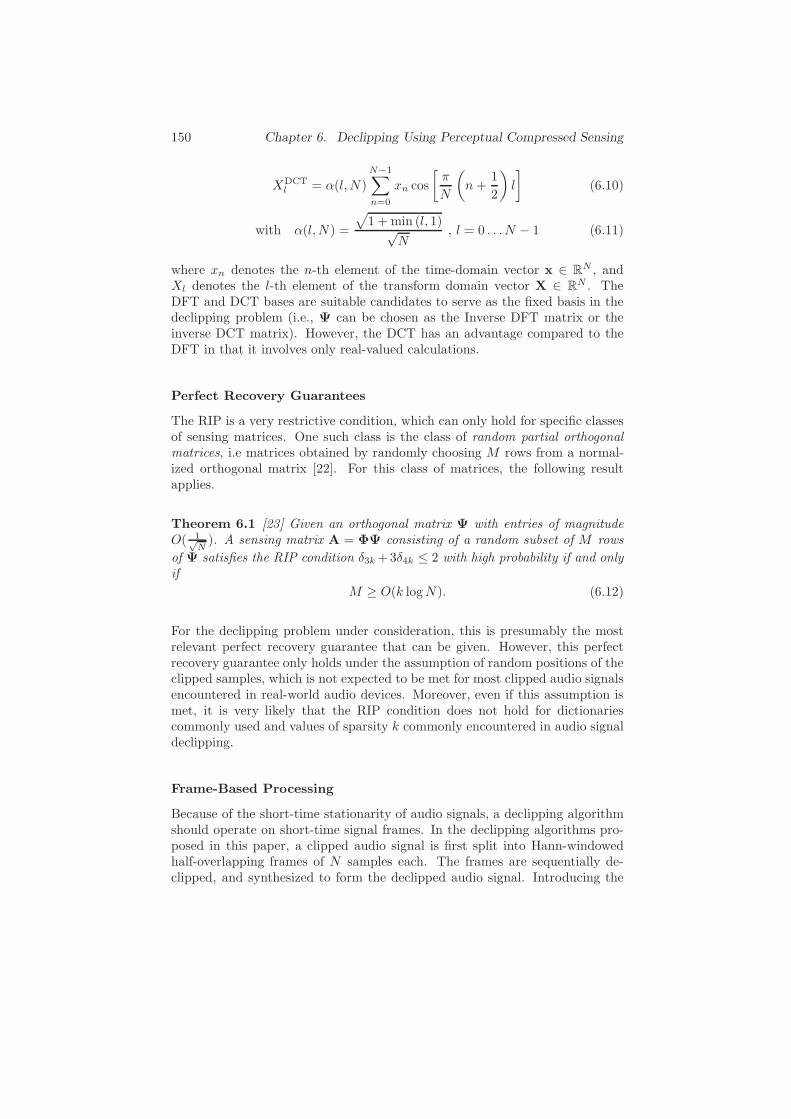
150 Chapter 6. Declipping Using Perceptual Compressed Sensing
XDCTl = α(l, N)
N−1∑
n=0
xn cos
[π
N
(
n+1
2
)
l
]
(6.10)
with α(l, N) =
√
1 + min (l, 1)√N
, l = 0 . . .N − 1 (6.11)
where xn denotes the n-th element of the time-domain vector x ∈ RN , and
Xl denotes the l-th element of the transform domain vector X ∈ RN . TheDFT and DCT bases are suitable candidates to serve as the fixed basis in thedeclipping problem (i.e., Ψ can be chosen as the Inverse DFT matrix or theinverse DCT matrix). However, the DCT has an advantage compared to theDFT in that it involves only real-valued calculations.
Perfect Recovery Guarantees
The RIP is a very restrictive condition, which can only hold for specific classesof sensing matrices. One such class is the class of random partial orthogonalmatrices, i.e matrices obtained by randomly choosing M rows from a normal-ized orthogonal matrix [22]. For this class of matrices, the following resultapplies.
Theorem 6.1 [23] Given an orthogonal matrix Ψ with entries of magnitudeO( 1√
N). A sensing matrix A = ΦΨ consisting of a random subset of M rows
of Ψ satisfies the RIP condition δ3k+3δ4k ≤ 2 with high probability if and onlyif
M ≥ O(k logN). (6.12)
For the declipping problem under consideration, this is presumably the mostrelevant perfect recovery guarantee that can be given. However, this perfectrecovery guarantee only holds under the assumption of random positions of theclipped samples, which is not expected to be met for most clipped audio signalsencountered in real-world audio devices. Moreover, even if this assumption ismet, it is very likely that the RIP condition does not hold for dictionariescommonly used and values of sparsity k commonly encountered in audio signaldeclipping.
Frame-Based Processing
Because of the short-time stationarity of audio signals, a declipping algorithmshould operate on short-time signal frames. In the declipping algorithms pro-posed in this paper, a clipped audio signal is first split into Hann-windowedhalf-overlapping frames of N samples each. The frames are sequentially de-clipped, and synthesized to form the declipped audio signal. Introducing the

6.2. A CS Framework for Declipping 151
subscript m as the frame index, the recovery step (6.2) for the m-th frame canbe rewritten as
x′m = argmin
z
‖z‖p s.t. Amz = ΦmΨz = ym. (6.13)
Alternative Recovery Step
The structure of a clipped audio signal has an inherent advantage, pertainingto the CS recovery step. As mentioned before, when applying a clipping levelθc to a signal, all sample values beyond θc are mapped onto θc. This meansthat the original value of any clipped sample is in absolute value larger than orequal to θc. This forms an additional constraint on the eligible solution spacefor the sparse recovery [7], which leads to the following recovery step,
x′m = argmin
z
‖z‖p s.t.
Amz = ΦmΨz = ym
C+mΨz ≥ θc
C−mΨz ≤ −θc
(6.14)
where C+m and C−
m are submatrices of an identity matrix where the rows corre-sponding to positively and negatively clipped samples, are respectively selected.Adding these constraints to the optimization problem is expected to improvethe signal recovery quality.
Relaxation of Equality Constraints
When the signal s is not exactly sparse but only compressible, as it is the casefor most real-world audio signals, a certain relaxation to the equality constraintsAmz = ym is desirable [24]. For ℓ0-norm minimization, a possible relaxationis to solve the following optimization problem,
x′m = argmin
z
‖z‖0 s.t.
‖ym −Amz‖22 ≤ ǫm
C+mΨz ≥ θc
C−mΨz ≤ −θc
(6.15)
where the value of the parameter ǫm > 0 should be carefully selected [7]. Asopposed to the ℓ0-norm minimization based declipping algorithms presented in[7], we will focus on the use of ℓ1-norm minimization for the declipping of audiosignals. When using ℓ1-norm minimization, the relaxation proposed here is tosolve the following optimization problem,
x′m = argmin
z
‖z‖1 +1
2γm‖ym −Amz‖22 s.t.
C+mΨz ≥ θc
C−mΨz ≤ −θc
(6.16)
where γm > 0 is a regularisation parameter. It is interesting to note thatthis optimization problem is similar to the well-known Basis Pursuit Denoisingproblem [17], except for the additional inequality constraints.

152 Chapter 6. Declipping Using Perceptual Compressed Sensing
Perceptual
model
Sparse signal recoveryyMx1 S’Nx1
tNx1
(a)
Perceptual
model
Sparse signal recoveryyMx1 S’Nx1
tNx1
(b)
Figure 6.2: Schematic overview of perceptual compressed sensing: (a) Feedfor-ward mode (b) Feedback mode. The symbol ∆ denotes a one-frame delay.
6.3 A PCS Framework for Declipping
In Section 6.2, the CS framework has been shown to be a suitable frameworkfor addressing the declipping problem. However, of crucial importance for au-dio applications is the resulting perceived audio quality of the declipped signal,which does not necessarily coincide with the physical signal reconstruction qual-ity. By additionally incorporating knowledge of human auditory perception, anovel perceptual compressed sensing (PCS) framework is presented in Subsec-tions 6.3.1 and 6.3.2. A PCS-based declipping algorithm, using ℓ1-norm typereconstruction, is presented in Subsection 6.3.3.
6.3.1 Perceptual CS Framework
It is known that audio signal components at certain frequencies are more per-ceptible than components at other frequencies, and that the relative perceptibil-ity is partly signal-dependent. Two phenomena of human auditory perceptionare responsible for this:
• The absolute threshold of hearing is defined as the required intensity (dB)of a pure tone such that an average listener will just hear the tone in anoiseless environment. The absolute threshold of hearing is a function of

6.3. A PCS Framework for Declipping 153
0 100 200 300 400 500−0.15
−0.1
−0.05
0
0.05
0.1
0.15
Time (n)
Am
plit
ude
(a)
0 5000 10000 15000 20000−10
0
10
20
30
40
50
60
Frequency (Hz)
SP
L(d
B)
(b)
0 5000 10000 15000 20000−10
0
10
20
30
40
50
60
Frequency (Hz)
SP
L(d
B)
(c)
0 5000 10000 15000 20000−10
0
10
20
30
40
50
60
Frequency (Hz)
SP
L(d
B)
(d)
0 5000 10000 15000 20000−10
0
10
20
30
40
50
60
Frequency (Hz)
SP
L(d
B)
(e)
0 5000 10000 15000 20000−10
0
10
20
30
40
50
60
Frequency (Hz)
SP
L(d
B)
(f)
0 5000 10000 15000 20000−10
0
10
20
30
40
50
60
Frequency (Hz)
SP
L(d
B)
(g)
Figure 6.3: Different steps in the computation of the global masking thresholdusing the ISO/IEC 11172-3 MPEG-1 Layer 1 psychoacoustic model 1 : (a)-(b)Time domain and normalized frequency domain representations of the inputaudio signal (c)-(d) Tonal maskers (circles), non-tonal maskers (squares) andinput frequency spectrum (dotted line) (e)-(f) Individual masking thresholdsrelated to tonal and non-tonal maskers respectively (g) Global masking thresh-old (solid line) and input frequency spectrum (dotted line) [11].

154 Chapter 6. Declipping Using Perceptual Compressed Sensing
the tone frequency and has been measured experimentally [25].• Simultaneous masking is a phenomenon where the presence of certain
spectral energy (the masker) masks the simultaneous presence of weakerspectral energy (the maskee), or in other words, renders it imperceptible.
Combining both phenomena, the instantaneous global masking threshold t ofan audio signal gives the amount of signal energy (dB) at each frequency thatcan be masked by the rest of the signal. As such, the masking threshold t givesan indication of the relative perceptibility of signal components at differentfrequencies, and can be used in the CS framework in order to focus on therecovery of perceptually important signal components, while at the same timeavoiding audible recovery errors.
Figure 6.2(a) gives a schematic overview of perceptual compressed sensing infeedforward mode. First, from the measurement y, the masking threshold t isestimated through the use of a perceptual model. Second, the sparse signal re-covery step uses the measurement y in conjunction with the masking thresholdt in order to recover the signal s′.
In practice, calculating the masking threshold t based on the measurement y,may not yield an accurate estimate of the masking threshold of the originalsignal s. Therefore, an alternative feedback mode of perceptual compressedsensing is proposed and illustrated in Figure 6.2(b). In feedback mode, themasking threshold tm for a current frame ym is computed from the declippedsignal s′m−1 of the previous frame. In the declipping algorithm proposed insubsection 6.3.3, perceptual compressed sensing will be used in feedback mode.The implications of this feedback masking threshold estimation procedure onthe declipping performance will be evaluated in Subsection 6.4.3.
6.3.2 Masking Threshold Calculation
The instantaneous global masking threshold t of a given audio signal is cal-culated using part of the ISO/IEC 11172-3 MPEG-1 Layer 1 psychoacousticmodel 1. A complete description of the operation of this psychoacoustic modelis beyond the scope of this paper (we refer the reader to [26] and [27]). We out-line the relevant steps in the computation of the instantaneous global maskingthreshold and illustrate the result of each step on an example audio signal (seeFigure 6.3):
1. Spectral analysis and SPL normalization: In this step a high-resolutionspectral estimate of the audio signal is calculated, with spectral compo-nents expressed in terms of sound pressure level (SPL). After a normal-ization operation and a Hann windowing operation on the input signalframe, the PSD estimate is obtained through a 512-point DFT. Fig-ure 6.3(a) shows the time-domain input signal, Figure 6.3(b) shows the
6.3. A PCS Framework for Declipping 155
resulting spectral estimate.2. Identification of tonal and non-tonal maskers : It is known from psy-
choacoustic research that the tonality of a masking component has aninfluence on its masking properties [28]. For this reason it is importantto discriminate between tonal maskers (defined as local maxima of thesignal spectrum) and non-tonal maskers. The output of the DFT is usedto determine the relevant tonal and non-tonal maskers in the spectrumof the audio signal. In a first phase, tonal maskers are identified atlocal maxima of the PSD: energy from three adjacent spectral compo-nents centered at the local maximum is combined to form a single tonalmasker. In a second phase, a single non-tonal masker per critical bandis formed by addition of all the energy from the spectral componentswithin the critical band that have not contributed to a tonal masker.
3. Decimation of maskers : In this step, the number of maskers is reducedusing two criteria. First, any tonal or non-tonal masker below the ab-solute threshold of hearing is discarded. Next, any pair of maskers oc-curring within a distance of 0.5 Bark is replaced by the stronger of thetwo. Figures 6.3(c) and 6.3(d) depict the identified tonal and non-tonalmaskers respectively, after decimation.
4. Calculation of individual masking thresholds : an individual maskingthreshold is calculated for each masker in the decimated set of tonaland non-tonal maskers, using fixed psychoacoustic rules. Essentially,the individual masking threshold depends on the frequency, loudnesslevel and tonality of the masker. Figure 6.3(e) and 6.3(f) show the indi-vidual masking thresholds associated with tonal and non-tonal maskers,respectively.
5. Calculation of global masking threshold : Finally, the global maskingthreshold is calculated by a power-additive combination of the tonal andnon-tonal individual masking thresholds, and the absolute threshold ofhearing. This is illustrated in Figure 6.3(g).
6.3.3 PCS-Based Declipping Using ℓ1-norm Optimization
In order to focus CS-based declipping on the recovery of perceptually relevantsignal components while at the same time avoiding audible recovery errors, themasking threshold will be incorporated into the CS recovery step. The proposedapproach is to introduce in the optimization problem a diagonal perceptualweighting matrix where the diagonal elements are the reciprocal of the maskingthreshold, hence indicating the relative perceptual importance of the differentsignal components. The perceptual weighting matrix Pm ∈ RN×N is defined
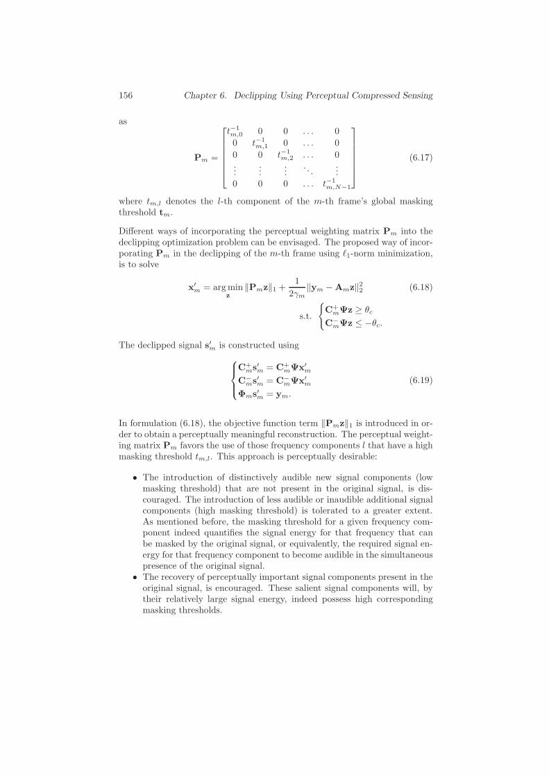
156 Chapter 6. Declipping Using Perceptual Compressed Sensing
as
Pm =
t−1m,0 0 0 . . . 0
0 t−1m,1 0 . . . 0
0 0 t−1m,2 . . . 0
......
.... . .
...0 0 0 . . . t−1
m,N−1
(6.17)
where tm,l denotes the l-th component of the m-th frame’s global maskingthreshold tm.
Different ways of incorporating the perceptual weighting matrix Pm into thedeclipping optimization problem can be envisaged. The proposed way of incor-porating Pm in the declipping of the m-th frame using ℓ1-norm minimization,is to solve
x′m = argmin
z
‖Pmz‖1 +1
2γm‖ym −Amz‖22 (6.18)
s.t.
C+mΨz ≥ θc
C−mΨz ≤ −θc.
The declipped signal s′m is constructed using
C+ms′m = C+
mΨx′m
C−ms′m = C−
mΨx′m
Φms′m = ym.
(6.19)
In formulation (6.18), the objective function term ‖Pmz‖1 is introduced in or-der to obtain a perceptually meaningful reconstruction. The perceptual weight-ing matrix Pm favors the use of those frequency components l that have a highmasking threshold tm,l. This approach is perceptually desirable:
• The introduction of distinctively audible new signal components (lowmasking threshold) that are not present in the original signal, is dis-couraged. The introduction of less audible or inaudible additional signalcomponents (high masking threshold) is tolerated to a greater extent.As mentioned before, the masking threshold for a given frequency com-ponent indeed quantifies the signal energy for that frequency that canbe masked by the original signal, or equivalently, the required signal en-ergy for that frequency component to become audible in the simultaneouspresence of the original signal.
• The recovery of perceptually important signal components present in theoriginal signal, is encouraged. These salient signal components will, bytheir relatively large signal energy, indeed possess high correspondingmasking thresholds.

6.4. Evaluation 157
Algorithm 8 (PCSL1)
Input ym ∈ RM , s′m−1 ∈ RN , Ψ ∈ CN×N , θc ∈ R+, γm ∈ R+
Output s′m ∈ RN
1: Srm = l||ym,l| < θc2: S+m = l|ym,l = θc3: S−m = l|ym,l = −θc4: Φm = IN (Srm)5: C+
m = IN (S+m)6: C−
m = IN (S−m)7: Am = ΦmΨ8: Calculate tm based on s′m−1 [using MPEG-1 Layer 1 psychoacoustic model
1]9: Determine Pm using (6.17)
10: Recover s′m by solving (6.18) and evaluating (6.19)
The perceptual weighting that is applied to the components of the sparsedecomposition can be alternatively interpreted in the framework of BayesianCompressive Sensing [29]. Omitting the constraints, the optimization problemin (6.18) is seen to be equivalent to a maximum a posteriori (MAP) formulationusing independent Laplace priors [30] for each basis coefficient in z, with meanprior values scaled by the corresponding diagonal elements of the perceptualweighting matrix Pm.
Algorithm 8 describes the different steps of the proposed PCSL1 algorithmfor declipping the m-th frame of a clipped audio signal, using ℓ1-norm typereconstruction.
6.4 Evaluation
In order to comparatively evaluate the designed declipping algorithm with re-spect to existing declipping algorithms, objective tests as well as subjectivelistening tests have been conducted. The set-up, results and interpretation ofthe conducted objective and subjective experiments will be discussed in thissection.
6.4.1 Objective Evaluation
To evaluate the declipping algorithms, two objective measures are used. A firstmeasure ∆SNR indicates the physical declipping improvement and is defined
In Algorithm 8, the notation IN (S) is introduced to denote a matrix consisting of thoserows of an N ×N identity matrix IN corresponding to the row indices in the index set S.
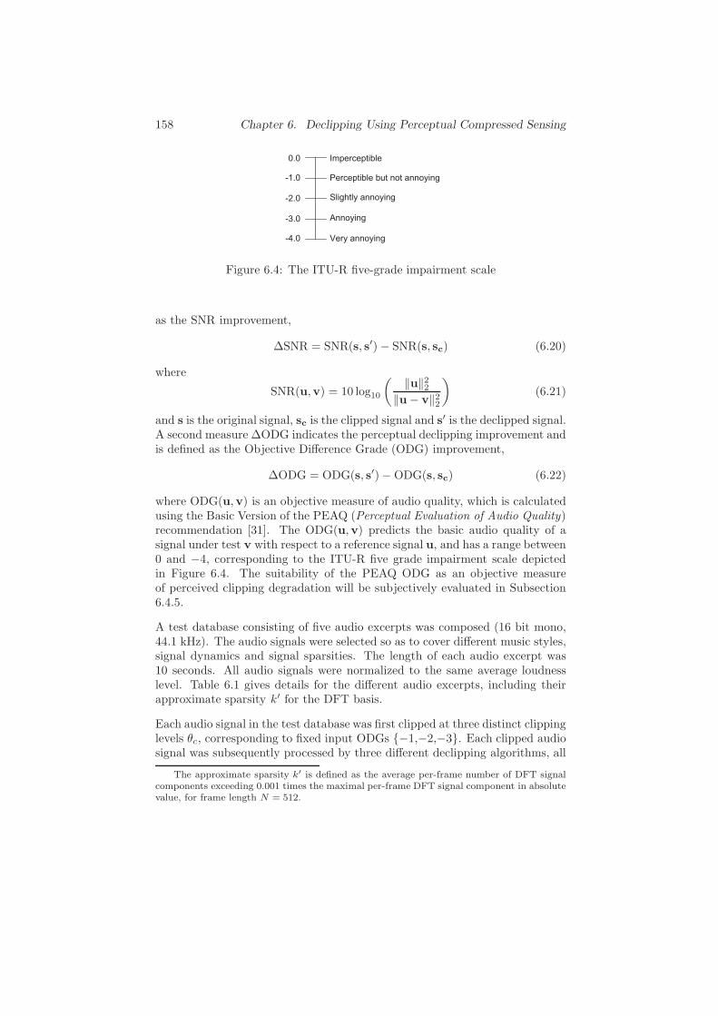
158 Chapter 6. Declipping Using Perceptual Compressed Sensing
0.0
-1.0
-2.0
-3.0
-4.0
Imperceptible
Perceptible but not annoying
Slightly annoying
Annoying
Very annoying
Figure 6.4: The ITU-R five-grade impairment scale
as the SNR improvement,
∆SNR = SNR(s, s′)− SNR(s, sc) (6.20)
where
SNR(u,v) = 10 log10
( ‖u‖22‖u− v‖22
)
(6.21)
and s is the original signal, sc is the clipped signal and s′ is the declipped signal.A second measure ∆ODG indicates the perceptual declipping improvement andis defined as the Objective Difference Grade (ODG) improvement,
∆ODG = ODG(s, s′)−ODG(s, sc) (6.22)
where ODG(u,v) is an objective measure of audio quality, which is calculatedusing the Basic Version of the PEAQ (Perceptual Evaluation of Audio Quality)recommendation [31]. The ODG(u,v) predicts the basic audio quality of asignal under test v with respect to a reference signal u, and has a range between0 and −4, corresponding to the ITU-R five grade impairment scale depictedin Figure 6.4. The suitability of the PEAQ ODG as an objective measureof perceived clipping degradation will be subjectively evaluated in Subsection6.4.5.
A test database consisting of five audio excerpts was composed (16 bit mono,44.1 kHz). The audio signals were selected so as to cover different music styles,signal dynamics and signal sparsities. The length of each audio excerpt was10 seconds. All audio signals were normalized to the same average loudnesslevel. Table 6.1 gives details for the different audio excerpts, including theirapproximate sparsity k′ for the DFT basis.
Each audio signal in the test database was first clipped at three distinct clippinglevels θc, corresponding to fixed input ODGs −1,−2,−3. Each clipped audiosignal was subsequently processed by three different declipping algorithms, all
The approximate sparsity k′ is defined as the average per-frame number of DFT signalcomponents exceeding 0.001 times the maximal per-frame DFT signal component in absolutevalue, for frame length N = 512.
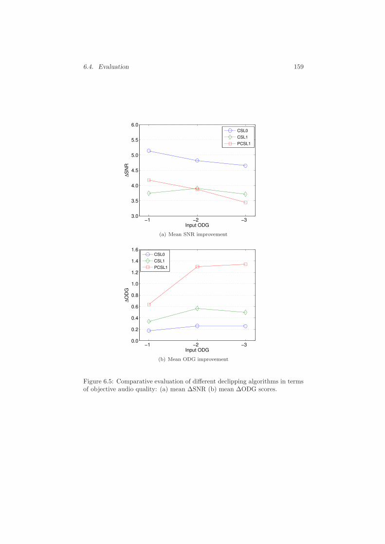
6.4. Evaluation 159
−1 −2 −33.0
3.5
4.0
4.5
5.0
5.5
6.0
Input ODG
∆S
NR
CSL0
CSL1
PCSL1
(a) Mean SNR improvement
−1 −2 −30.0
0.2
0.4
0.6
0.8
1.0
1.2
1.4
1.6
Input ODG
∆O
DG
CSL0
CSL1
PCSL1
(b) Mean ODG improvement
Figure 6.5: Comparative evaluation of different declipping algorithms in termsof objective audio quality: (a) mean ∆SNR (b) mean ∆ODG scores.
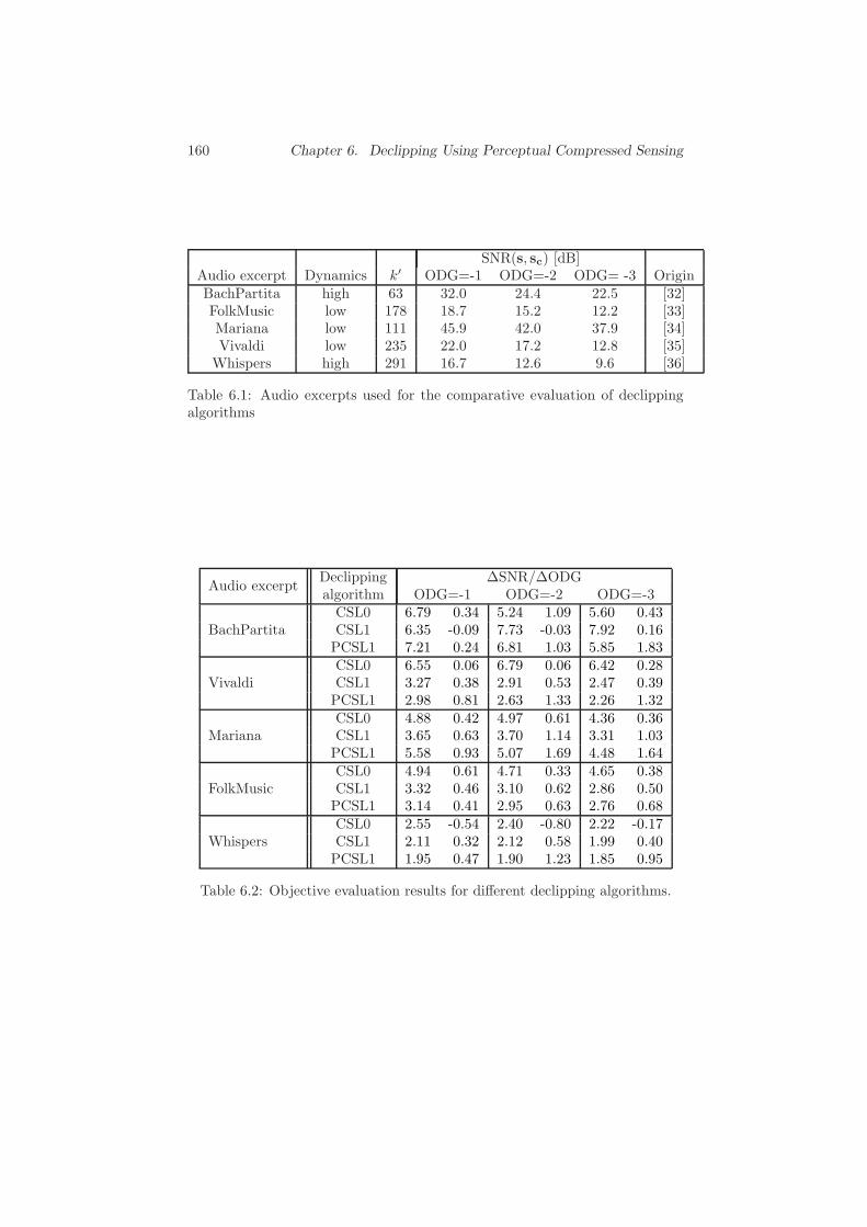
160 Chapter 6. Declipping Using Perceptual Compressed Sensing
SNR(s, sc) [dB]Audio excerpt Dynamics k′ ODG=-1 ODG=-2 ODG= -3 OriginBachPartita high 63 32.0 24.4 22.5 [32]FolkMusic low 178 18.7 15.2 12.2 [33]Mariana low 111 45.9 42.0 37.9 [34]Vivaldi low 235 22.0 17.2 12.8 [35]Whispers high 291 16.7 12.6 9.6 [36]
Table 6.1: Audio excerpts used for the comparative evaluation of declippingalgorithms
Audio excerptDeclipping ∆SNR/∆ODGalgorithm ODG=-1 ODG=-2 ODG=-3
BachPartitaCSL0 6.79 0.34 5.24 1.09 5.60 0.43CSL1 6.35 -0.09 7.73 -0.03 7.92 0.16PCSL1 7.21 0.24 6.81 1.03 5.85 1.83
VivaldiCSL0 6.55 0.06 6.79 0.06 6.42 0.28CSL1 3.27 0.38 2.91 0.53 2.47 0.39PCSL1 2.98 0.81 2.63 1.33 2.26 1.32
MarianaCSL0 4.88 0.42 4.97 0.61 4.36 0.36CSL1 3.65 0.63 3.70 1.14 3.31 1.03PCSL1 5.58 0.93 5.07 1.69 4.48 1.64
FolkMusicCSL0 4.94 0.61 4.71 0.33 4.65 0.38CSL1 3.32 0.46 3.10 0.62 2.86 0.50PCSL1 3.14 0.41 2.95 0.63 2.76 0.68
WhispersCSL0 2.55 -0.54 2.40 -0.80 2.22 -0.17CSL1 2.11 0.32 2.12 0.58 1.99 0.40PCSL1 1.95 0.47 1.90 1.23 1.85 0.95
Table 6.2: Objective evaluation results for different declipping algorithms.
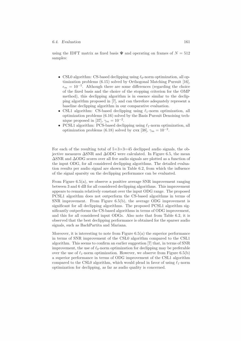
6.4. Evaluation 161
using the IDFT matrix as fixed basis Ψ and operating on frames of N = 512samples:
• CSL0 algorithm: CS-based declipping using ℓ0-norm optimization, all op-timization problems (6.15) solved by Orthogonal Matching Pursuit [16],ǫm = 10−5. Although there are some differences (regarding the choiceof the fixed basis and the choice of the stopping criterion for the OMPmethod), this declipping algorithm is in essence similar to the declip-ping algorithm proposed in [7], and can therefore adequately represent abaseline declipping algorithm in our comparative evaluation.
• CSL1 algorithm: CS-based declipping using ℓ1-norm optimization, alloptimization problems (6.16) solved by the Basis Pursuit Denoising tech-nique proposed in [37], γm = 10−2.
• PCSL1 algorithm: PCS-based declipping using ℓ1-norm optimization, alloptimization problems (6.18) solved by cvx [38], γm = 10−2.
For each of the resulting total of 5×3×3=45 declipped audio signals, the ob-jective measures ∆SNR and ∆ODG were calculated. In Figure 6.5, the mean∆SNR and ∆ODG scores over all five audio signals are plotted as a function ofthe input ODG, for all considered declipping algorithms. The detailed evalua-tion results per audio signal are shown in Table 6.2, from which the influenceof the signal sparsity on the declipping performance can be evaluated.
From Figure 6.5(a), we observe a positive average SNR improvement rangingbetween 3 and 6 dB for all considered declipping algorithms. This improvementappears to remain relatively constant over the input ODG range. The proposedPCSL1 algorithm does not outperform the CS-based algorithms in terms ofSNR improvement. From Figure 6.5(b), the average ODG improvement issignificant for all declipping algorithms. The proposed PCSL1 algorithm sig-nificantly outperforms the CS-based algorithms in terms of ODG improvement,and this for all considered input ODGs. Also note that from Table 6.2, it isobserved that the best declipping performance is obtained for the sparser audiosignals, such as BachPartita and Mariana.
Moreover, it is interesting to note from Figure 6.5(a) the superior performancein terms of SNR improvement of the CSL0 algorithm compared to the CSL1algorithm. This seems to confirm an earlier suggestion [7] that, in terms of SNRimprovement, the use of ℓ0-norm optimization for declipping may be preferableover the use of ℓ1-norm optimization. However, we observe from Figure 6.5(b)a superior performance in terms of ODG improvement of the CSL1 algorithmcompared to the CSL0 algorithm, which would plead in favor of using ℓ1-normoptimization for declipping, as far as audio quality is concerned.

162 Chapter 6. Declipping Using Perceptual Compressed Sensing
10e1 10e0 10e−1 10e−2 10e−3 10e−4
−1.5
−1
−0.5
0
γm
OD
Gre
l
ODG=−1
ODG=−2
ODG=−3
(a) Vivaldi
10e1 10e0 10e−1 10e−2 10e−3 10e−4
−1.5
−1
−0.5
0
γm
OD
Gre
l
ODG=−1
ODG=−2
ODG=−3
(b) Whispers
Figure 6.6: Impact of the regularisation parameter γm in the PCSL1 declippingalgorithm on the resulting relative (to the maximum) ODG score, for differentinput ODGs: (a) “Vivaldi” (b) “Whispers”.

6.4. Evaluation 163
6.4.2 Impact of Regularisation Parameter γm
In [7], it was shown that the parameter ǫm in the CSL0 optimization formulation(6.15) should be carefully selected, as the resulting SNR improvement wasseen to be very sensitive to the value of ǫm. Based upon these findings andsome additional experiments, we have selected ǫm = 10−5 as an appropriateparameter setting for the experiments discussed in Subsection IV-A.
In order to study the impact of the regularisation parameter γm in the PCSL1optimization formulation (6.18) on the resulting audio quality, the followingexperiment was conducted. Each of the five audio signals in the test databasedetailed in Table 6.1 were clipped at three distinct clipping levels, correspondingto fixed input ODGs −1,−2,−3. These signals were subsequently processedby the PCSL1 declipping algorithm using optimization formulation (6.18), inwhich the value of the regularisation parameter γm was fixed over all frameswithin one audio signal, and this processing was repeated for six different valuesof γm = 101,100,10−1, 10−2,10−3,10−4. For each of the resulting total of5×3×6=90 declipped audio signals, the ODG between the original signal andthe declipped signal was calculated.
The results of this experiment are partly visualized in Figure 6.6, which showsthe results for the audio excerpts “Vivaldi” and “Whispers”. In these figures,the objective measure ODGrel, defined as
ODGrel(γm) = ODG(γm)−maxγm
ODG(γm) (6.23)
is plotted as a function of γm, and this for different input ODGs. We observethat the choice of γm has a significant impact on the resulting audio qualityscores after declipping and this regardless of the input ODG, so care should betaken when selecting the value of γm. Moreover, we observe that the differentcurves reach a joint maximum for γm = 10−2. We have selected γm = 10−2 asan experimentally validated setting for our experiments discussed in Subsection6.4.1.
6.4.3 Impact of Masking Threshold Estimation Proce-
dure
In Section 6.3, the estimation of the masking threshold was discussed. It wasproposed to estimate the masking threshold tm for a current signal frame ym bycomputing it from the previously declipped signal frame s′m−1. The impact ofthis feedback masking threshold estimation procedure on the PCSL1 declippingperformance has been evaluated as follows.
The audio signals “Vivaldi” and “Whispers” (see test database detailed inTable 6.1) were clipped at three distinct clipping levels, corresponding to fixedinput ODGs −1,−2,−3. These signals were subsequently processed by the
164 Chapter 6. Declipping Using Perceptual Compressed Sensing
PCSL1 declipping algorithm, in which the per-frame masking thresholds wereestablished using two different procedures:
• Ideal masking threshold: the per-frame masking threshold was calculatedusing the clean signal frame sm. Using this ideal masking thresholdprovides an upper bound for the declipping performance of the PCSL1algorithm.
• Estimated masking treshold: the per-frame masking threshold tm wascomputed using the previously declipped signal frame s′m−1, as detailedin Algorithm 8.
The results of this experiment are shown in Figure 6.7. It can be observed thatfor both audio excerpts, the resulting ∆ODG scores using the estimated mask-ing threshold in the declipping algorithm, are very close to the upper boundsprovided by using the ideal masking threshold. These results indicate that theuse of the proposed masking treshold estimation procedure does not have asignificant negative impact on the resulting objective audio quality scores.
6.4.4 Subjective Evaluation
Research question and hypothesis
The research question to be answered through performing a formal subjec-tive listening test [39] is the following: “how does the perceived audio qualityimprovement of audio signals declipped by the proposed PCSL1 algorithm com-pare to that of audio signals declipped by the CSL0 and CSL1 algorithms?”.The research hypothesis, that may or may not be rejected, is that the perceivedaudio quality improvement is identical for all three declipping algorithms.
Test subjects
A representative sample of 16 test subjects having considerable musical listen-ing and performance experience was selected to perform the listening test. Allsubjects were remunerated for their participation.
Experimental design and set-up
The listening tests were performed in a soundproof and well-illuminated testroom. Stimuli were presented to the test subjects through high-quality circum-aural headphones connected to a soundcard-equipped laptop. Self-developed
Sennheiser HD 439: dynamic, closed transducer, frequency response 17-22500Hz, SoundPressure Level 112 dB, Total Harmonic Distortion < 0.1%.
Sony Vaio VGN-CR41: Intel Core 2 duo T5550 processor @1.83Ghz, 3GB RAM, Realteksound card, Intel GMA X3100 Graphics Processor.

6.4. Evaluation 165
−1 −2 −30.4
0.5
0.6
0.7
0.8
0.9
1.0
1.1
1.2
1.3
1.4
Input ODG
∆O
DG
Estimated MT
Ideal MT
(a) Vivaldi
−1 −2 −30.4
0.5
0.6
0.7
0.8
0.9
1.0
1.1
1.2
1.3
1.4
Input ODG
∆O
DG
Estimated MT
Ideal MT
(b) Whispers
Figure 6.7: Impact of the masking threshold estimation procedure in the PCSL1declipping algorithm on the ∆ODG score, for different input ODGs: (a) “Vi-valdi” (b) “Whispers”.
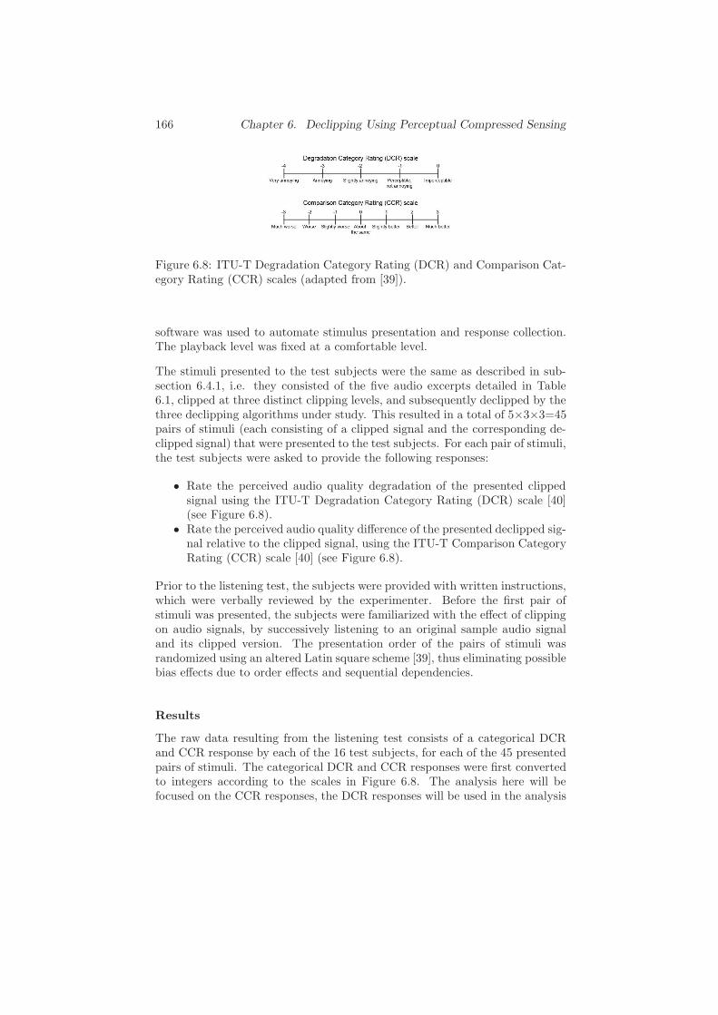
166 Chapter 6. Declipping Using Perceptual Compressed Sensing
Figure 6.8: ITU-T Degradation Category Rating (DCR) and Comparison Cat-egory Rating (CCR) scales (adapted from [39]).
software was used to automate stimulus presentation and response collection.The playback level was fixed at a comfortable level.
The stimuli presented to the test subjects were the same as described in sub-section 6.4.1, i.e. they consisted of the five audio excerpts detailed in Table6.1, clipped at three distinct clipping levels, and subsequently declipped by thethree declipping algorithms under study. This resulted in a total of 5×3×3=45pairs of stimuli (each consisting of a clipped signal and the corresponding de-clipped signal) that were presented to the test subjects. For each pair of stimuli,the test subjects were asked to provide the following responses:
• Rate the perceived audio quality degradation of the presented clippedsignal using the ITU-T Degradation Category Rating (DCR) scale [40](see Figure 6.8).
• Rate the perceived audio quality difference of the presented declipped sig-nal relative to the clipped signal, using the ITU-T Comparison CategoryRating (CCR) scale [40] (see Figure 6.8).
Prior to the listening test, the subjects were provided with written instructions,which were verbally reviewed by the experimenter. Before the first pair ofstimuli was presented, the subjects were familiarized with the effect of clippingon audio signals, by successively listening to an original sample audio signaland its clipped version. The presentation order of the pairs of stimuli wasrandomized using an altered Latin square scheme [39], thus eliminating possiblebias effects due to order effects and sequential dependencies.
Results
The raw data resulting from the listening test consists of a categorical DCRand CCR response by each of the 16 test subjects, for each of the 45 presentedpairs of stimuli. The categorical DCR and CCR responses were first convertedto integers according to the scales in Figure 6.8. The analysis here will befocused on the CCR responses, the DCR responses will be used in the analysis

6.4. Evaluation 167
in Subsection 6.4.5. Let us denominate the averaged CCR responses over all 16test subjects as CCR responses, and the averaged CCR responses over all five
audio excerpts as CCR responses. In Figure 6.9, the CCR responses are plottedas a function of the input ODG level, and this for the three different declippingalgorithms under study. We observe that the ranking of the algorithms isidentical to the one observed in the objective evaluation results in Figure 6.5(b).The detailed CCR responses per audio excerpt are given in Table 6.3.
The following statistical analysis was performed on the obtained numerical setof CCR responses. Let us denote the population CCR responses correspondingto audio signals declipped by the CSL0, CSL1 and PCSL1 algorithms by ran-dom variables RCSL0, RCSL1, and RPCSL1, respectively. Based on the sampleCCR responses, we tested the following three statistical hypotheses H0 againsttheir alternatives Ha,
H10 : RCSL0 = RPCSL1 (6.24)
H1a : RCSL0 ≤ RPCSL1 (6.25)
H20 : RCSL1 = RPCSL1 (6.26)
H2a : RCSL1 ≤ RPCSL1 (6.27)
H30 : RCSL0 = RCSL1 (6.28)
H3a : RCSL0 ≤ RCSL1 (6.29)
where R is the population median of the random variable R. These threestatistical hypotheses were tested for all three considered input ODGs. Allstatistical hypotheses were tested using one-tailed Wilcoxon-Mann-Whitneytests [41] with significance level α = 0.05. The resulting one-sided P-values aresynthesized in Table 6.4.
The first null hypothesis (6.24) can be rejected in favor of the alternative (6.25)for all considered input ODGs. The second and third null hypotheses (6.26)and (6.28) can be rejected in favor of their respective alternatives (6.27) and(6.29) for input ODGs of -2 and -3.
Conclusions
The research hypothesis can be confidently rejected, i.e. the perceived audioquality improvement is not identical for all three declipping algorithms. Thestatistical analysis has shown that the PCSL1 algorithm delivers a significantlybetter audio quality improvement than both the CSL0 algorithm (for all input

168 Chapter 6. Declipping Using Perceptual Compressed Sensing
−1 −2 −30.0
0.2
0.4
0.6
0.8
1.0
1.2
1.4
1.6
Input ODG
CC
R
CSL0
CSL1
PCSL1
Figure 6.9: Comparative evaluation of different declipping algorithms in terms
of the CCR responses.
Audio excerptDeclipping CCRalgorithm ODG=-1 ODG=-2 ODG=-3
BachPartitaCSL0 0.44 0.38 0.63CSL1 0.38 0.38 0.75PCSL1 1.63 2.56 2.31
VivaldiCSL0 0.25 0.75 0.44CSL1 0.38 0.69 0.94PCSL1 0.38 0.88 1.56
MarianaCSL0 0.81 0.63 0.31CSL1 1.38 1.81 1.19PCSL1 1.69 2.19 2.06
FolkMusicCSL0 0.63 0.44 0.75CSL1 0.50 1.13 1.25PCSL1 0.44 1.19 1.06
WhispersCSL0 1.31 1.13 1.06CSL1 1.69 0.94 1.13PCSL1 1.06 1.19 0.88
Table 6.3: Subjective evaluation results for different declipping algorithms.
Table 6.4: P-values from one-tailed Wilcoxon-Mann-Whitney tests on sampleCCR responses. Significant P-values with respect to α = 0.05 in bold.
Null hypothesis → H10 H2
0 H30
ODG=-1 0.0202 0.2006 0.1313ODG=-2 <0.0001 0.0003 0.0178
ODG=-3 <0.0001 0.0004 0.0035
6.5. Conclusions 169
ODGs) and the CSL1 algorithm (for input ODGs in -2,-3). Moreover, theCSL1 algorithm delivers a significantly better perceived audio quality improve-ment than the CSL0 algorithm (for input ODGs in -2,-3).
6.4.5 Suitability of PEAQ ODG as a Measure of Per-
ceived Clipping Degradation
The PEAQ ODG measure has been developed in the context of quality evalu-ation of low-bit-rate encoded audio. As the nature of signal distortions intro-duced by clipping can be rather different as compared to signal distortions in-troduced by low-bit-rate codecs, the use of PEAQODG as an objective measureof perceived clipping-induced degradations should be well-founded. Therefore,we have investigated the appropriateness of the PEAQ ODG measure for quan-tifying the perceived clipping-induced audio quality degradation by analyzingthe DCR data collected in the listening test described in Subsection 6.4.4.
Let us denominate the averaged DCR responses over all 16 test subjects asDCR responses. In Figure 6.10, the DCR responses are plotted as a functionof the corresponding ODG score, and this for the five different audio excerpts.We observe a strong positive correlation between DCR responses and ODGscores, and this for all audio excerpts. Moreover, the different curves are seento be monotonously increasing and they do not deviate excessively from linearcurves. The different curves do have a noticeably different vertical offset, buthave a nearly equal slope. These results seem to indicate that the ODGmeasurecan be confidently used to compare the perceived clipping-induced audio qualitydegradation for the same audio excerpt in different processing scenarios (as wasdone in Subsection 6.4.1). However, it might not be advisable to use the ODGmeasure to compare the perceived clipping-induced audio quality degradationfor different audio excerpts.
6.5 Conclusions
In this paper, a novel perceptual compressed sensing (PCS) framework hasbeen presented for declipping audio signals, in which the theory of compressedsensing (CS) was combined with properties of human auditory perception. Adeclipping algorithm using ℓ1-norm type reconstruction has been developed inthe PCS framework. Comparative evaluation experiments consisting of objec-tive and subjective tests have revealed a significant audio quality increase ofthe proposed PCS-based declipping algorithm compared to CS-based declip-ping algorithms for reasonably sparse signals.
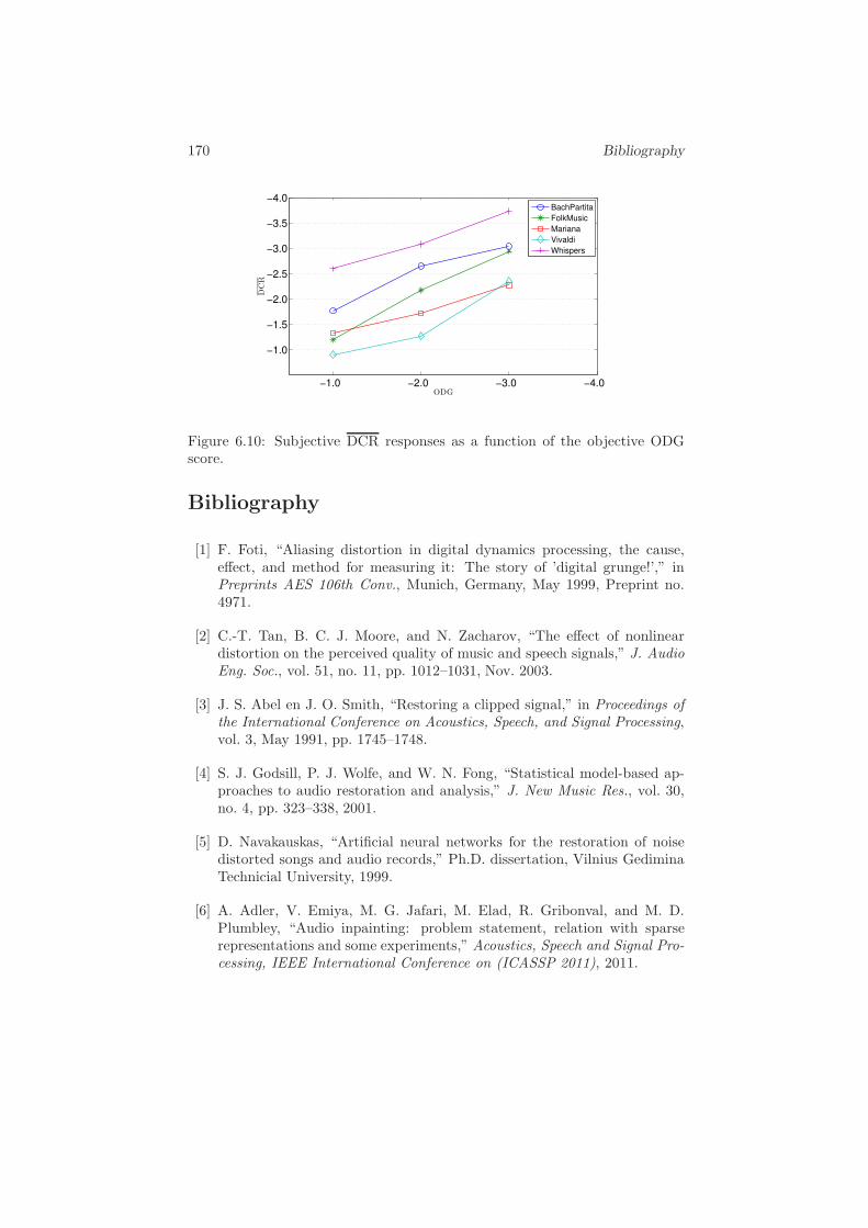
170 Bibliography
−1.0 −2.0 −3.0 −4.0
−1.0
−1.5
−2.0
−2.5
−3.0
−3.5
−4.0
DC
R
ODG
BachPartita
FolkMusic
Mariana
Vivaldi
Whispers
Figure 6.10: Subjective DCR responses as a function of the objective ODGscore.
Bibliography
[1] F. Foti, “Aliasing distortion in digital dynamics processing, the cause,effect, and method for measuring it: The story of ’digital grunge!’,” inPreprints AES 106th Conv., Munich, Germany, May 1999, Preprint no.4971.
[2] C.-T. Tan, B. C. J. Moore, and N. Zacharov, “The effect of nonlineardistortion on the perceived quality of music and speech signals,” J. AudioEng. Soc., vol. 51, no. 11, pp. 1012–1031, Nov. 2003.
[3] J. S. Abel en J. O. Smith, “Restoring a clipped signal,” in Proceedings ofthe International Conference on Acoustics, Speech, and Signal Processing,vol. 3, May 1991, pp. 1745–1748.
[4] S. J. Godsill, P. J. Wolfe, and W. N. Fong, “Statistical model-based ap-proaches to audio restoration and analysis,” J. New Music Res., vol. 30,no. 4, pp. 323–338, 2001.
[5] D. Navakauskas, “Artificial neural networks for the restoration of noisedistorted songs and audio records,” Ph.D. dissertation, Vilnius GediminaTechnicial University, 1999.
[6] A. Adler, V. Emiya, M. G. Jafari, M. Elad, R. Gribonval, and M. D.Plumbley, “Audio inpainting: problem statement, relation with sparserepresentations and some experiments,” Acoustics, Speech and Signal Pro-cessing, IEEE International Conference on (ICASSP 2011), 2011.

171
[7] ——, “Audio inpainting,” IEEE Transactions on Audio, Speech and Lan-guage Processing, 2011.
[8] A. J. Weinstein and M. B. Waking, “Recovering a clipped signal in sparse-land,” Sampling Theory in Signal and Image Processing, to appear.
[9] C. Studer, P. Kuppinger, G. Pope, and H. Bolcskei, “Recovery of sparselycorrupted signals,” IEEE Transactions on Information Theory, vol. 58,no. 5, pp. 3115–3130, May 2012.
[10] M. Christensen and B. Sturm, “A perceptually reweighted mixed-normmethod for sparse approximation of audio signals,” in 2011 ConferenceRecord of the Forty Fifth Asilomar Conference on Signals, Systems andComputers (ASILOMAR), Nov. 2011, pp. 575 –579.
[11] B. Defraene, T. van Waterschoot, H. J. Ferreau, M. Diehl, and M. Moo-nen, “Real-time perception-based clipping of audio signals using convexoptimization,” IEEE Transactions on Audio, Speech, and Language Pro-cessing, vol. 20, no. 10, pp. 2657 –2671, Dec. 2012.
[12] E. Candes, J. Romberg, and T. Tao, “Robust uncertainty principles : Ex-act signal reconstruction from highly incomplete frequency information,”IEEE Trans. on Information Theory, vol. 52, no. 2, pp. 489–509, 2006.
[13] E. Candes and T. Tao, “Near optimal signal recovery from random pro-jections: Universal encoding strategies?” IEEE Trans. Inform. Theory,vol. 52, no. 12, p. 54065425, 2006.
[14] D. Donoho, “Compressed sensing,” IEEE Trans. on Information Theory,vol. 52, no. 4, pp. 1289–1306, 2006.
[15] M. D. Plumbley, T. Blumensath, L. Daudet, R. Gribonval, and M. E.Davies, “Sparse representations in audio and music: from coding to sourceseparation,” Proceedings of the IEEE, vol. 98, no. 6, pp. 995–1005, 2010.
[16] Y. C. Pati, R. Rezaiifar, and P. S. Krishnaprasad, “Orhogonal matchingpursuit: Recursive function approximation with applications to waveletdecomposition,” In Proc. Annual Asilomar Conference on signals, systemsand computers, 1993.
[17] S. S. Chen, D. L. Donoho, and M. A. Saunders, “Atomic decompositionby basis pursuit,” SIAM journal on scientific computing, vol. 20, no. 1,pp. 33–61, 1998.
[18] E. Candes and T. Tao, “The dantzig selector: Statistical estimation whenp is much larger than n,” The Annals of Statistics, vol. 35, no. 6, pp.2313–2351, 2007.

172 Bibliography
[19] E. Candes, J. Romberg, and T. Tao, “Stable signal recovery from incom-plete and inaccurate measurements,” Communications on pure and appliedmathematics, vol. 59, no. 8, pp. 1207–1223, 2006.
[20] Y. C. Eldar and G. Kutyniok, Compressed sensing: theory and applica-tions. Cambridge University Press, 2012.
[21] D. L. Donoho and M. Elad, “Optimally sparse representation in general(nonorthogonal) dictionaries via l1 minimization,” Proceedings of the Na-tional Academy of Sciences, vol. 100, no. 5, pp. 2197–2202, 2003.
[22] L. Gan, C. Lingy, T. Doz, and T. Tranz, “Analysis of the statistical re-stricted isometry property for deterministic sensing matrices using steinsmethod,” [Online], http://dsp.rice.edu/?les/cs/GanStatRIP.pdf 2009.
[23] M. Rudelson and R. Vershynin, “On sparse reconstruction from fourier andgaussian measurements,” Communications on Pure and Applied Mathe-matics, vol. 61, no. 8, pp. 1025–1045, 2008.
[24] J. Yang and Y. Zhang, “Alternating direction algorithms for ℓ1-problemsin compressive sensing,” SIAM journal on scientific computing, vol. 33,no. 1, pp. 250–278, 2011.
[25] E. Terhardt, “Calculating virtual pitch,” Hearing Res., vol. 1, no. 2, pp.155 – 182, 1979.
[26] T. Painter and A. Spanias, “Perceptual coding of digital audio,” Proc.IEEE, vol. 88, no. 4, pp. 451–515, Apr. 2000.
[27] ISO/IEC, “11172-3 Information technology - Coding of moving picturesand associated audio for digital storage media at up to about 1.5 Mbit/s- Part 3: Audio,” 1993.
[28] E. Zwicker and H. Fastl, Psychoacoustics: facts and models, 2nd ed.Springer, 1999.
[29] S. Ji, Y. Xue, and L. Carin, “Bayesian compressive sensing,” IEEE Trans-actions on Signal Processing, vol. 56, no. 6, pp. 2346–2356, 2008.
[30] S. D. Babacan, R. Molina, and A. K. Katsaggelos, “Bayesian compressivesensing using laplace priors,” IEEE Transactions on Image Processing,vol. 19, no. 1, pp. 53–63, 2010.
[31] International Telecommunications Union Recommendation BS.1387,“Method for objective measurements of perceived audio quality,” 1998.
[32] J. S. Bach, “Partita no. 3 in a minor(1),” bWV 826.
[33] Naragonia, “Martin-Pecheur & Pink Molly,” Tandem.
173
[34] August Burns Red, “Marianas Trench,” Constellations, Solid StateRecords.
[35] A. Vivaldi, “The Four Seasons - Spring,” rV 269.
[36] All That Remains, “Whispers (I Hear Your),” The Fall of Ideals, Pros-thetic Records.
[37] K. M. Cheman, “Optimization techniques for solving basis pursuit prob-lems,” Ph.D. dissertation, North Carolina State University, 2006.
[38] M. Grant, S. Boyd, and Y. Ye, “Cvx: Matlab software for disciplinedconvex programming,” Online accessible: http://stanford. edu/˜ boyd/cvx,2008.
[39] S. Bech and N. Zacharov, Perceptual audio evaluation-Theory, method andapplication. Wiley, 2007.
[40] International Telecommunications Union Recommendation P. 800, “Meth-ods for subjective determination of transmission quality,” 1996.
[41] F. Wilcoxon, “Individual comparisons by ranking methods,” Biometricsbulletin, vol. 1, no. 6, pp. 80–83, 1945.

174 Bibliography
Chapter 7
Multi-Microphone
Dereverberation
Embedded Optimization Algorithms for
Multi-Microphone Dereverberation
Toon van Waterschoot, Bruno Defraene, Moritz Diehl,
and Marc Moonen
Published in Proc. of the 21st European Signal Process. Conf.(EUSIPCO ’13), Marrakech, Morocco, Sept. 2013.
175

176 Chapter 7. Multi-Microphone Dereverberation
Contributions of second author
• literature review• co-analysis of multi-microphone dereverberation problem• co-development of embedded optimization problem formula-
tion• co-design of evaluation experiments• co-interpretation of simulation results• co-formulation of conclusions• text co-editing and co-revision

7.1. Introduction 177
Abstract
In this paper we propose a new approach to multi-microphone dereverberation,based on the recent paradigm of embedded optimization. The rationale of em-bedded optimization in performing online signal processing tasks is to replacetraditional adaptive filtering algorithms based on closed-form estimators byfast numerical algorithms solving constrained and potentially non-convex opti-mization problems. In the context of dereverberation, we adopt the embeddedoptimization paradigm to arrive at a joint estimation of the source signal ofinterest and the unknown room acoustics. It is shown how the inherently non-convex joint estimation problem can be smoothed by including regularizationterms based on a statistical late reverberation model and a sparsity prior forthe source signal spectrum. A performance evaluation for an example multi-microphone dereverberation scenario shows promising results, thus motivatingfuture research in this direction.
7.1 Introduction
Dereverberation refers to the process of removing reverberation from micro-phone signals recorded in a reverberant room. Since reverberation often has afundamental impact on the time-frequency signal characteristics, dereverber-ation has been found to be a crucial component in diverse speech and audioapplications, such as hearing assistance, automatic speech recognition, voicecommunications, and acoustic surveillance. Despite its wide applicability, dere-verberation is generally still considered one of the most challenging problemsin the area of acoustic signal enhancement [1]. One of the major difficulties isthat dereverberation is an inverse problem, i.e., one aims at inverting the roomimpulse response (RIR), which is typically non-minimum-phase and possiblytime-varying. Furthermore, dereverberation is usually also a blind problem, inwhich both the sound source signal and the room acoustics are unknown.
The state of the art in speech dereverberation can be classified into three cat-egories [1, Ch. 1]: (1) beamforming, (2) speech enhancement, and (3) blindsystem identification and inversion. Most of the existing methods rely on theuse of multiple microphones. This is implictly the case for the beamforming ap-proaches which are based on microphone array processing, see, e.g., [2]. Speechenhancement approaches to dereverberation have also been shown to benefitfrom the use of multiple microphones, e.g., for accurately estimating the latereverberant signal spectrum [3] or for enhancing a linear prediction residual byspatiotemporal averaging [4]. Finally, blind system identification is typicallybased on the cross-relation between different microphone signals [5], while theinversion of a non-minimum-phase system has been shown to be feasible onlyin the multi-channel case [6].

178 Chapter 7. Multi-Microphone Dereverberation
In this paper, a different approach to dereverberation is proposed, which doesnot exactly fit into one of the three categories mentioned earlier. The proposedapproach is somehow related to the blind system identification and inversionapproach, however, it differs in that it does not require an explicit systeminversion. Indeed, the major weakness of the blind system identification andinversion approach is that the design of a (multi-channel) inverse filter oftenappears to be an ill-posed problem, which may be due to (near-)common zeros[7] or system identification errors [8] in the RIRs. Recent solutions to alleviatethis weakness are based on modifications in the inverse filter design, such assubband inversion [9], regularization [10], and forced spectral diversity [11].
Instead, we propose to avoid an explicit system inversion by adopting a re-cent paradigm coined as embedded optimization. This paradigm is based onthe observation that the field of numerical optimization has reached a degreeof maturity and computational efficiency such that it can be applied to onlinesignal processing problems that are traditionally solved using recursive imple-mentations of “classical” estimators admitting a closed-form solution [12]. Inparticular, it allows to directly estimate a signal vector of interest, rather thantaking a detour by designing a filter to recover a signal of interest from noisyor corrupted observations.
The outline of this paper is as follows. In Section 7.2 we propose a relevantsignal model and formulate the multi-microphone dereverberation problem. InSection 7.3 we propose a number of embedded optimization algorithms formulti-microphone dereverberation. These algorithms are evaluated in Section7.4 for a simple example scenario. Finally, Section 7.5 concludes the paper.
7.2 Problem Statement
Consider a point source emitting a sound signal s0(t), t = 1, . . . , N , whichpropagates inside a room and is picked up by M microphones at differentpositions. The resulting microphone signals (m = 1, . . . ,M) are defined as
ym(t) = hTm,0(t)s0(t) + em,0(t), t = 1, . . . , N (7.1)
where the length-L RIR vector hm,0(t) from the source to the mth microphoneat time t is defined as
hm,0(t) =[
h(0)m,0(t) . . . h
(L−1)m,0 (t)
]T
, t = 1, . . . , N (7.2)
the length-L source signal vector s0(t) at time t is defined as
s0(t) =[s0(t) . . . s0(t− L+ 1)
]T, t = 1, . . . , N (7.3)
and em,0(t), t = 1, . . . , N , denotes measurement noise.

7.2. Problem Statement 179
In this paper, we make a number of assumptions that may not be valid inrealistic sound acquisition scenarios, but which will allow us (1) to focus onthe core issues encountered in the dereverberation problem, postponing somepractical and implementation issues to future work (see Section 7.5), and (2) toinvestigate and interpret the proposed algorithms’ behavior only w.r.t. thesecore issues, disregarding the potential impact of other issues on the algorithmperformance. The assumptions are the following (with m = 1, . . . ,M):
• microphone signals are available for the entire time window t ∈ [1, N ]under consideration;
• RIRs are time-invariant within the time window t ∈ [1, N ] under consid-eration, i.e., hm,0(t) ≡ hm,0;
• initial source signal conditions s0(t), t ≤ 0 are known (and assumed equalto zero for ease of notation);
• no measurement noise is present, i.e., em,0(t) ≡ 0;• all RIRs have equal and known length L ≤ N .
Based on these assumptions, the problem considered in this paper can be for-mulated as follows:
Problem 1 (Multi-microphone dereverberation) Given a length-MN vec-tor of microphone signals generated as
y = H0s0 (7.4)
find the best possible estimate of the length-N source signal vector s0. Here,with m = 1, . . . ,M ,
y =[yT1 . . . yT
M
]T, ym =
[ym(1) . . . ym(N)
]T(7.5)
H0 =[HT
1,0 . . . HTM,0
]T(7.6)
Hm,0 =
h(0)m,0 0 0 . . . 0...
. . .. . .
. . ....
h(L−1)m,0 . . . h
(0)m,0
. . . 0...
. . ....
. . . 0
0 . . . h(L−1)m,0 . . . h
(0)m,0
N×N
(7.7)
s0 =[s0(1) . . . s0(N)
]T. (7.8)
Since the RIRs in H0 as well as the source signal vector s0 are unknown, wedefine the following parameter vectors,
h =[hT1 . . . hT
M
]T, hm =
[
h(0)m . . . h
(L−1)m
]T
(7.9)

180 Chapter 7. Multi-Microphone Dereverberation
s =[s(1) . . . s(N)
]T(7.10)
e =[eT1 . . . eTM
]T, em =
[em(1) . . . em(N)
]T(7.11)
and a data model admitting two equivalent formulations,
y = Hs+ e (7.12)
= (IM ⊗ S)h+ e (7.13)
where H is a MN × N matrix with the coefficients of the RIRs parametervector h in a block Toeplitz structure as in (7.6)-(7.7), IM is the M × Midentity matrix, ⊗ denotes the Kronecker product, and S is a N × L Toeplitzmatrix defined as
S =
s(1) . . . 0...
. . ....
s(N − L+ 1) . . . s(1)...
. . ....
s(N) . . . s(N − L+ 1)
. (7.14)
The error signal parameter vector e is included to account for estimation errorsin both h and s.
7.3 Embedded Optimization Algorithms
State-of-the-art multi-microphone dereverberation algorithms in the categoryof blind system identification and inversion approach Problem 1 using a two-step procedure. First, an estimate H of the RIRs matrix is computed using ablind identification method that typically exploits the cross-relation betweendifferent microphone signals [5]. Second, an M -input, single-output inversefilter g is designed and an estimate of the source signal vector is obtained as
s = Gy (7.15)
where G is a block Toeplitz matrix of appropriate dimensions, containing theinverse filter coefficients in g.
Instead, we propose to jointly estimate the RIRs parameter vector h and thesource signal parameter vector s. We derive three nonlinear least squares (NLS)optimization problems for estimating h and s, and point out their strengthsand weaknesses. More particularly, we consider NLS problems without regu-larization (NLS), with ℓ2-norm regularization exploiting prior knowledge onh (ℓ2-RNLS), and with ℓ1-norm and ℓ2-norm regularization exploiting priorknowledge on s and h (ℓ1/ℓ2-RNLS). A block coordinate descent (BCD) ap-proach is adopted for solving these problems, resulting in three iterative algo-rithms in which h and s are estimated sequentially.

7.3. Embedded Optimization Algorithms 181
The sequential nature of the proposed algorithms shows a certain degree ofsimilarity with the state-of-the-art two-step procedure for blind system iden-tification and inversion. A crucial difference, however, is that the RIRs pa-rameter vector h is not just estimated once, but its estimate is iterativelyrefined as improved estimates of the source signal parameter vector becomeavailable. Another similarity with the state of the art, is that the source signalparameter vector estimate resulting from the NLS and ℓ2-RNLS problems islinearly related to the microphone signal vector y, so that it can be interpretedas the result of an inverse filtering approach, even though an inverse filter isnever explicitly designed or computed. When solving the ℓ1/ℓ2-RNLS problem,however, the source signal parameter vector estimate is not linearly related tothe microphone signal vector and so an inverse filtering interpretation is notappropriate.
7.3.1 NLS problem
The starting point for the derivation of embedded optimization algorithmssolving Problem 1, is the formulation of an NLS optimization problem for thedata model (7.12)-(7.13),
minh,s,e
‖e‖22 (7.16)
s. t. y = Hs+ e (7.17)
= (IM ⊗ S)h+ e. (7.18)
The proposed solution strategy consists in first minimizing (7.16) w.r.t. s, efor a fixed value of h = h using the equality constraints in (7.17), then minimiz-ing (7.16) w.r.t. h, e for a fixed value of s = s using the equality constraintsin (7.18), and repeating this procedure for a number of iterations (here fixedto kmax). The resulting BCD algorithm is shown in Algorithm 9, where (·)+denotes the Moore-Penrose pseudoinverse.
Algorithm 9 BCD algorithm for NLS problem
Input initial RIRs parameter vector estimate h(0)
Output parameter vector estimates s = s(kmax), h = h(kmax)
1: for k = 1, . . . , kmax do2: s(k) = (H(k−1))+y
3: h(k) =(
IM ⊗ (S(k))+)
y
4: end for
7.3.2 ℓ2-regularized NLS problem
It is well known that the NLS optimization problem in (7.16)-(7.18) generallyhas multiple local solutions, and the BCD algorithm will only converge to
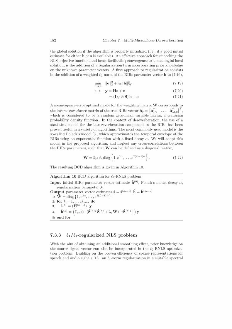
182 Chapter 7. Multi-Microphone Dereverberation
the global solution if the algorithm is properly initialized (i.e., if a good initialestimate for either h or s is available). An effective approach for smoothing theNLS objective function, and hence facilitating convergence to a meaningful localsolution, is the addition of a regularization term incorporating prior knowledgeon the unknown parameter vectors. A first approach to regularization consistsin the addition of a weighted ℓ2-norm of the RIRs parameter vector h to (7.16),
minh,s,e
‖e‖22 + λ1‖h‖2W (7.19)
s. t. y = Hs+ e (7.20)
= (IM ⊗ S)h+ e (7.21)
A mean-square-error optimal choice for the weighting matrix W corresponds to
the inverse covariance matrix of the true RIRs vector h0 =[hT1,0 . . . hT
M,0
]T,
which is considered to be a random zero-mean variable having a Gaussianprobability density function. In the context of dereverberation, the use of astatistical model for the late reverberation component in the RIRs has beenproven useful in a variety of algorithms. The most commonly used model is theso-called Polack’s model [3], which approximates the temporal envelope of theRIRs using an exponential function with a fixed decay α. We will adopt thismodel in the proposed algorithm, and neglect any cross-correlations betweenthe RIRs parameters, such that W can be defined as a diagonal matrix,
W = IM ⊗ diag
1, e2α, . . . , e2(L−1)α
. (7.22)
The resulting BCD algorithm is given in Algorithm 10.
Algorithm 10 BCD algorithm for ℓ2-RNLS problem
Input initial RIRs parameter vector estimate h(0), Polack’s model decay α,regularization parameter λ1
Output parameter vector estimates s = s(kmax), h = h(kmax)
1: W = diag1, e2α, . . . , e2(L−1)α
2: for k = 1, . . . , kmax do3: s(k) = (H(k−1))+y
4: h(k) =(
IM ⊗[(S(k)T S(k) + λ1W)−1S(k)T
])
y
5: end for
7.3.3 ℓ1/ℓ2-regularized NLS problem
With the aim of obtaining an additional smoothing effect, prior knowledge onthe source signal vector can also be incorporated in the ℓ2-RNLS optimiza-tion problem. Building on the proven efficiency of sparse representations forspeech and audio signals [13], an ℓ1-norm regularization in a suitable spectral

7.4. Evaluation 183
basis seems to be appropriate for this purpose. When combined with the ℓ2-norm regularization of the RIRs parameter vector, this results in the followingoptimization problem,
minh,s,e
‖e‖22 + λ1‖h‖2W + λ2‖Ds‖1 (7.23)
s. t. y = Hs+ e (7.24)
= (IM ⊗ S)h+ e. (7.25)
Here, D is an N ×N orthogonal matrix defining a spectral transform, such asthe discrete Fourier or cosine transform (DFT/DCT). In contrast to the pre-vious two problems, the optimization problem in (7.23)-(7.25) does not admita closed-form solution when optimizing w.r.t. s, e. However, this particu-lar subproblem is convex and can therefore be efficiently solved using existingsoftware (e.g., we use CVX/SeDuMi). The resulting BCD algorithm is shownin Algorithm 11.
Algorithm 11 BCD algorithm for ℓ1/ℓ2-RNLS problem
Input initial RIRs parameter vector estimate h(0), Polack’s model decay α,orthogonal spectral transform matrix D, regularization parameters λ1, λ2
Output parameter vector estimates s = s(kmax), h = h(kmax)
1: W = diag1, e2α, . . . , e2(L−1)α
2: for k = 1, . . . , kmax do3: s(k) = argmins ‖y − H(k−1)s‖22 + λ2‖Ds‖14: h(k) =
(
IM ⊗[(S(k)T S(k) + λ1W)−1S(k)T
])
y
5: end for
7.4 Evaluation
The proposed embedded optimization algorithms for multi-microphone dere-verberation are evaluated here by means of a simulation example. A micro-phone signal vector y is generated by filtering a source signal vector s0 of lengthN = 1024, corresponding to a quasi-stationary voiced segment of a male speechsignal sampled at 8 kHz, using M = 5 synthetic RIRs of length L = 100. TheRIRs are synthesized by shapingM = 5 different Gaussian white noise (GWN)sequences with an exponential envelope corresponding to Polack’s model withα = 0.025. The same envelope is used for designing the weighting matrix W inthe ℓ2-RNLS and ℓ1/ℓ2-RNLS problems. The regularization parameters havebeen chosen as λ1 = λ2 = 0.1, and D is the DCT matrix. All algorithmsstart from a random GWN initial RIRs parameter vector estimate h(0) andperform kmax = 10 iterations. In the simulation results, the inherent scalingambiguity has been removed by plotting s/a and ah rather than s and h, with
a =√
sT s/sT0 s0.
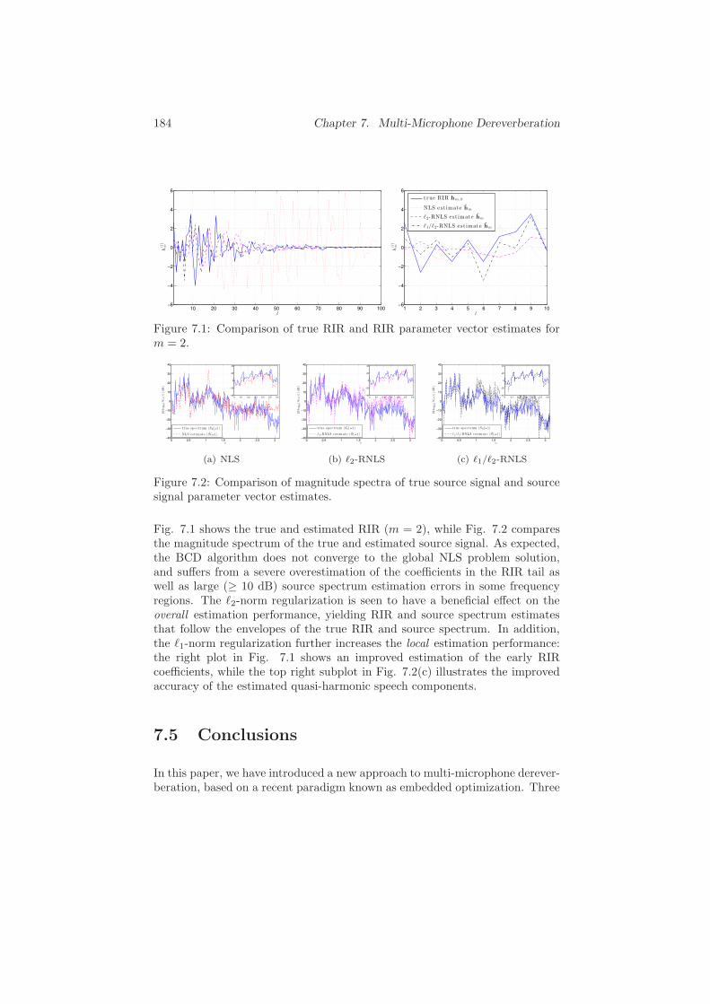
184 Chapter 7. Multi-Microphone Dereverberation
10 20 30 40 50 60 70 80 90 100−6
−4
−2
0
2
4
6
l
h(l)
m
1 2 3 4 5 6 7 8 9 10−6
−4
−2
0
2
4
6
l
h(l)
m
true RIR hm, 0
NLS est imate hm
ℓ2-RNLS est imate hm
ℓ1/ℓ2-RNLS est imate hm
Figure 7.1: Comparison of true RIR and RIR parameter vector estimates form = 2.
0 0.5 1 1.5 2 2.5 3−40
−30
−20
−10
0
10
20
30
40
ω
20log 1
0|S
(ω)|
(dB)
true spectrum |S0(ω) |
NLS est imate | S(ω) |
0 0.1 0.2 0.3 0.4 0.5 0.6−40
−20
0
20
40
(a) NLS
0 0.5 1 1.5 2 2.5 3−40
−30
−20
−10
0
10
20
30
40
ω
20log 1
0|S
(ω)|
(dB)
true spectrum |S0(ω) |
ℓ2-RNLS est imate | S(ω) |
0 0.1 0.2 0.3 0.4 0.5 0.6−40
−20
0
20
40
(b) ℓ2-RNLS
0 0.5 1 1.5 2 2.5 3−40
−30
−20
−10
0
10
20
30
40
ω
20log 1
0|S
(ω)|
(dB)
true spectrum |S0(ω) |
ℓ1/ℓ2-RNLS est imate | S(ω) |
0 0.1 0.2 0.3 0.4 0.5 0.6−40
−20
0
20
40
(c) ℓ1/ℓ2-RNLS
Figure 7.2: Comparison of magnitude spectra of true source signal and sourcesignal parameter vector estimates.
Fig. 7.1 shows the true and estimated RIR (m = 2), while Fig. 7.2 comparesthe magnitude spectrum of the true and estimated source signal. As expected,the BCD algorithm does not converge to the global NLS problem solution,and suffers from a severe overestimation of the coefficients in the RIR tail aswell as large (≥ 10 dB) source spectrum estimation errors in some frequencyregions. The ℓ2-norm regularization is seen to have a beneficial effect on theoverall estimation performance, yielding RIR and source spectrum estimatesthat follow the envelopes of the true RIR and source spectrum. In addition,the ℓ1-norm regularization further increases the local estimation performance:the right plot in Fig. 7.1 shows an improved estimation of the early RIRcoefficients, while the top right subplot in Fig. 7.2(c) illustrates the improvedaccuracy of the estimated quasi-harmonic speech components.
7.5 Conclusions
In this paper, we have introduced a new approach to multi-microphone derever-beration, based on a recent paradigm known as embedded optimization. Three

BIBLIOGRAPHY 185
sequential optimization algorithms have been proposed, which enable the jointestimation of the unknown source signal and room acoustics. By adopting aniterative numerical optimization strategy, the need for an explicit inverse filterdesign is avoided. However, the inclusion of appropriate regularization termsin the inherently non-convex optimization problem appears to be crucial for as-suring convergence to a meaningful local solution. In particular, the addition ofa weighted ℓ2-norm of the RIRs parameter vector, based on a statistical modelfor late reverberation, leads to an improved overall estimation performance. Inaddition, the accuracy of the estimated early reflections and (quasi-)harmonicsource signal components can be further increased by incorporating an ℓ1-normregularization term for the source signal parameter vector DFT/DCT.
The work presented in this paper is a first step towards the development ofefficient and reliable embedded optimization algorithms for multi-microphonedereverberation. A number of challenges for future research remain, e.g.,
• to move from batch to online (frame-based) processing, properly manag-ing initial/final conditions,
• to generalize the ℓ2-norm regularization for dealing with realistic impulseresponses,
• to take measurement noise into account,• to arrive at autonomous optimization algorithms involving proper termi-
nation criteria and cross-validation procedures for adjusting the regular-ization parameters,
• to derive fast SQP/SCP algorithms exploiting the particular dereverber-ation problem structure,
• to use perceptual criteria in the problem formulations,• to evaluate the resulting dereverberation performance.
Bibliography
[1] P. A. Naylor and N. D. Gaubitch, Eds., Speech dereverberation. London:Springer, 2010.
[2] J. L. Flanagan, A. C. Surendran, and E. E. Jan, “Spatially selective soundcapture for speech and audio processing,” vol. 13, no. 1–2, pp. 207–222,Oct. 1993.
[3] E. A. P. Habets, “Multi-channel speech dereverberation based on a sta-tistical model of late reverberation,” vol. 4, Philadelphia, PA, USA, Mar.2005, pp. 173–176.
[4] N. D. Gaubitch and P. A. Naylor, “Spatiotemporal averaging method forenhancement of reverberant speech,” Cardiff, UK, Jun. 2007, pp. 607–610.

186 Bibliography
[5] G. Xu, H. Liu, L. Tong, and T. Kailath, “A least-squares approach toblind channel identification,” vol. 43, no. 12, pp. 2982–2993, Dec. 1995.
[6] M. Miyoshi and Y. Kaneda, “Inverse filtering of room acoustics,” vol.ASSP-36, no. 2, pp. 145–152, Feb. 1988.
[7] W. Zhang and P. A. Naylor, “An experimental study of the robustness ofmultichannel inverse filtering systems to near-common zeros,” Glasgow,Scotland, UK, Aug. 2009, pp. 194–198.
[8] ——, “A system-identification-error-robust method for equalization ofmultichannel acoustic systems,” Dallas, TX, USA, Mar. 2010, pp. 109–112.
[9] N. D. Gaubitch and P. A. Naylor, “Equalization of multichannel acousticsystems in oversampled subbands,” vol. 17, no. 6, pp. 1061–1070, Aug.2009.
[10] I. Kodrasi, S. Goetze, and S. Doclo, “Increasing the robustness of acousticmultichannel equalization by means of regularization,” Aachen, Germany,Sep. 2012, pp. 161–164.
[11] X. S. Lin, A. W. H. Khong, and P. A. Naylor, “A forced spectral diver-sity algorithm for speech dereverberation in the presence of near-commonzeros,” vol. 20, no. 3, pp. 888–899, Mar. 2012.
[12] J. Mattingley and S. Boyd, “Real-time convex optimization in signal pro-cessing,” vol. 27, no. 3, pp. 50–61, May 2010.
[13] M. D. Plumbey, T. Blumensath, L. Daudet, R. Gribonval, and M. E.Davies, “Sparse representations in audio and music: from coding to sourceseparation,” vol. 98, no. 6, pp. 995–1005, 2010.

Chapter 8
Conclusions and
Suggestions for Future
Research
8.1 Summary and Conclusions
In this thesis we have designed an embedded optimization framework for au-dio signal enhancement and investigated its application to four different audiosignal enhancement problems, namely hard clipping precompensation, loud-speaker precompensation, declipping and multi-microphone dereverberation.The research objectives formulated in Chapter 1 were the conceptual develop-ment of an embedded optimization framework for audio signal enchancement,the incorporation of perceptual information into this framework, the designand hardware implementation of application-tailored optimization methods,and the comparative objective and subjective evaluation with state-of-the-artaudio signal enhancement algorithms. These research objectives have beenachieved, resulting in the following four major contributions of this thesis.
The first major contribution consists in the conceptual development of an em-bedded optimization framework and its application to different audio signal en-chancement problems. In a first part of this thesis, precompensation algorithmsfor audio signal enhancement have been considered. Hard clipping precompen-sation was formulated in Chapter 2 as a sequence of per-frame constrainedconvex quadratic optimization problems. Loudspeaker precompensation wasformulated in Chapter 3 as a sequence of per-frame nonconvex optimizationproblems, in which the loudspeaker was modeled by a grey-box Hammerstein
187
188 Chapter 8. Conclusions and Suggestions for Future Research
loudspeaker model, i.e. a cascade of a memoryless nonlinearity and a linear fi-nite impulse response filter. In a second part of this thesis, recovery algorithmsfor audio signal enhancement have been considered. Declipping was formu-lated in Chapter 6 as a sparse signal recovery problem in the DFT domain,in which the recovery was performed by solving a per-frame ℓ1-norm-type con-vex optimization problem. Multi-microphone dereverberation was formulatedin Chapter 7 as a nonconvex optimization problem, allowing for the jointestimation of the room acoustics model parameters and the clean audio signal.
The second major contribution of this thesis consists in the incorporation ofperceptual information into the embedded optimization algorithms through theuse of a model of human sound perception. In the proposed embedded optimiza-tion precompensation algorithms, the MPEG perceptual model [1] was appliedto compute the instantaneous masking threshold, in order to establish an objec-tive mathematical measure reflecting the perceptible distortion incurred in thesubsequent distortion process. In the hard clipping precompensation algorithmpresented in Chapter 2, an objective function reflecting the perceptible non-linear clipping distortion was constructed by including frequency weights basedon the instantaneous masking threshold. In the loudspeaker precompensationalgorithm presented in Chapter 3, an objective function reflecting the per-ceptible combined linear and nonlinear loudspeaker distortion was constructedin a similar fashion. In the declipping algorithm presented in Chapter 6, fre-quency weights based on the instantaneous masking threshold were includedin the ℓ1-norm optimization criterion. As a result, the declipping algorithmwas focused on maximizing the perceived audio quality of the declipped signalinstead of the physical signal reconstruction quality. In the multi-microphonedereverberation algorithm of Chapter 7, perceptual information was not ex-plicitly incorporated into the embedded optimization algorithm. However, theaddition of regularization terms based on a statistical late reverberation modeland a sparsity prior for the clean audio signal spectrum has shown that theoptimization problem formulation lends itself very well to the inclusion of priorinformation, which could be easily extended to the inclusion of perceptual in-formation.
The third major contribution of this thesis consists in the design and hard-ware implementation of fast and reliable optimization methods for solving theper-frame optimization problems. As concerns hard clipping precompensation,three different structure-exploiting convex optimization methods were proposedin Chapter 2 for solving the per-frame constrained convex quadratic opti-mization problems. A first method was an active set method, a second andthird method were projected gradient methods, for which theoretical complex-ity bounds were derived. The fastest of these optimization methods was seento be the optimal projected gradient method originally proposed in [2], whichwas shown to run in real time on a standard PC. The hardware implemen-tation of the optimal projected gradient optimization method on a field pro-

8.1. Summary and Conclusions 189
grammable gate array (FPGA) was discussed Chapter 5. Bit-accurate sim-ulations of the FPGA implementation have demonstrated that the transitionfrom floating-point arithmetic to fixed-point arithmetic and the selection ofthe corresponding bit width has an impact on the resulting audio quality aswell as on the resource usage and power consumption of the design. The se-lected FPGA design solves the per-frame optimization problems by performing30 optimal projected gradient iterations using 20 fixed-point fraction bits, hasa low latency, a reduced power consumption, a reduced resource usage, andat the same time preserves the full audio quality improvement. This designallows to perform the algorithm in real time on a small and portable audiodevice. In Chapter 3, the solution of the per-frame nonconvex optimizationproblems for loudspeaker precompensation was considered. Depending on theinvertibility and the smoothness of the memoryless nonlinearity in the Ham-merstein loudspeaker model, different optimization strategies were proposed.In the case of an invertible memoryless nonlinearity, the optimization problemwas seen to have a closed-form solution. In the case of a non-invertible smoothmemoryless nonlinearity, a gradient optimization method was applied, whereasfor non-invertible hard clipping memoryless nonlinearities, the optimal pro-jected gradient optimization method was applied. For the multi-microphonedereverberation algorithm discussed in Chapter 7, the resulting nonconvexjoint estimation problem was solved using a block coordinate descent (BCD)approach, sequentially estimating the room acoustics model parameters andthe clean audio signal.
The fourth major contribution of this thesis consists in the comparative ob-jective and subjective evaluation of the designed embedded optimization algo-rithms with state-of-the-art audio signal enhancement algorithms. For hardclipping precompensation, the objective audio quality evaluation performed inChapter 2 reported significantly higher objective audio quality scores usingthe embedded optimization algorithm over standard hard clipping precompen-sation techniques, and this for moderate to high levels of clipping. For loud-speaker precompensation, the objective evaluation experiments using syntheticand identified loudspeaker models performed in Chapter 3 have shown thatthe embedded optimization loudspeaker precompensation algorithm provides asignificant audio quality improvement, especially so at high loudspeaker play-back levels. In Chapter 4, a subjective evaluation of the aforementioned hardclipping and loudspeaker precompensation algorithms was performed, througha formal listening test including 19 test subjects. The conclusions of this sub-jective evaluation were seen to confirm the outcome of the objective evaluationexperiments. Moreover, some interesting side results were obtained from thesubjective evaluation experiments. First, the perceived audio quality of audiosignals subject to a certain nonlinear hard clipping distortion was seen to benot significantly superior to that of audio signals subject to the same nonlin-ear hard clipping distortion and an additional linear distortion. This confirmsearlier findings [3] that nonlinear distortion is dominant in the perception with

190 Chapter 8. Conclusions and Suggestions for Future Research
respect to linear distortion. Second, there was a significant positive correlationbetween subjective audio quality scores and objective audio quality scores,supporting the validity of using objective measures to assess the audio qualityof signals subject to hard clipping and loudspeaker distortion. In Chapter6, objective and subjective evaluation experiments (formal listening test us-ing 16 test subjects) have revealed a significant audio quality increase for theproposed embedded optimization declipping algorithm compared to existingCS-based declipping algorithms.
8.2 Suggestions for Future Research
In this thesis, precompensation algorithms and recovery algorithms for audiosignal enhancement have been considered in an embedded optimization frame-work. The dichotomy between precompensation and recovery algorithms wasintroduced due to the observation that in many cases, the audio signal can onlybe processed either before or after the distortion process acts onto the audiosignal. However, one can think of commonly encountered scenarios where theaudio signal can be processed both before and after the action of the distortionprocess, e.g. a predictable hard clipping distortion process, or a distortion pro-cess occuring during audio signal mastering or transmission stages. In thesescenarios, a precompensation algorithm and a recovery algorithm could coop-erate in order to maximally mitigate the perceptible effects of the distortionprocess. This joint integration of precompensation and recovery in an em-bedded optimization approach is in our view a highly interesting and relevantdirection for future research.
Next, the application of a model of human sound perception in the proposedembedded optimization framework was seen to result in an improved audioquality for hard clipping precompensation, loudspeaker precompensation anddeclipping problems. When the goal is to improve another perceptual attribute,such as speech quality or speech intelligibility, it will be necessary to incorporatea perceptual model translating these specific perceptual attributes to mathe-matical measures that can be optimized for. The study and integration ofthese perceptual models is an important step to allow the embedded optimiza-tion framework to maximally enhance these perceptual attributes. Moreover,whereas the focus of this thesis has been on improving human sound perception,it is our opinion that the embedded optimization approach is equally suited forapplications where the aim is to improve the sound perception by machines,e.g. in automatic speech recognition, given the proper inclusion of models ofmachine sound perception.
Concerning the fast and reliable solution of the per-frame optimization prob-lems that form the core of the embedded optimization algorithms, we have
8.2. Suggestions for Future Research 191
followed the path of exploiting as much as possible the inherent structure ofthe optimization problems. For the considered convex optimization problems,we have if possible also derived theoretical upper bounds on the algorithmiccomplexity. In this approach, the resulting application-specific optimizationmethods have to be implemented in or translated to compilable and reliablecode that can be embedded in real-time audio applications. We note that adifferent paradigm called automatic code generation [4] can be envisaged forperforming embedded optimization in real-time audio signal enhancement ap-plications. This approach takes a high-level description of an optimizationproblem family, and automatically generates code that compiles into a reliableand high-speed solver for the problem family. The exploration of automaticcode generation approaches for embedded optimization in audio signal enhance-ment applications and their comparison in terms of speed and reliability withthe optimization approach presented in this thesis forms a highly relevant topicfor future research.
Finally, we also want to point out that most of the proposed embedded opti-mization algorithms rely on an estimate of the model parameters of the dis-tortion process under consideration. However, the distortion model parameterestimation will in general not be performed without estimation errors. It istherefore worthwile to assess the sensitivity of the resulting audio signal en-hancement performance of the different embedded optimization algorithms toestimation errors in the distortion model parameters.
Beside the suggested general directions for future research discussed above,we can point out some potential research directions for the specific audio sig-nal enhancement problems of loudspeaker compensation and multi-microphonedereverberation.
Loudspeaker Precompensation
In this thesis, the loudspeaker has been modeled using a grey-box Hammersteinmodel, which gives a good trade-off between model accuracy and model com-plexity. The application of more complex loudspeaker models, such as Volterramodels or white-box lumped parameter models could result in a higher accu-racy in modeling the different loudspeaker distortion mechanisms. However,the precompensation of such loudspeaker models using embedded optimizationwill presumably result in more complex and typically nonconvex optimizationproblems. The adequate formulation and efficient solution of such optimizationproblems involving more complex loudspeaker models, and the comparison be-tween the precompensation performance for different loudspeaker models wouldform major contributions to the loudspeaker compensation problem.
Moreover, in this thesis the loudspeaker model parameters were estimated off-line during a separate estimation procedure. In practice, the loudspeaker model

192 Bibliography
parameters might vary over time, e.g. due to temperature changes. On-linetracking of the time variation of the loudspeaker model parameters is a chal-lenging problem due to the difficulty to properly feed back the reproduced audiosignal, which could be achieved using some form of measurement and feedbackof the loudspeaker voice coil displacement or temperature.
Multi-Microphone Dereverberation
In this thesis, an embedded optimization approach to multi-microphone dere-verberation has been presented, which was seen to differ fundamentally fromexisting dereverberation approaches. The promising results of this approachfor an example multi-microphone dereverberation scenario motivate future re-search in this direction. In our view, the most important research topics to beaddressed are the derivation of fast optimization methods exploiting the par-ticular dereverberation problem structure, the inclusion of measurement noise,the incorporation of perceptual criteria in the problem formulation, and theevaluation of the resulting dereverberation performance using objective andsubjective speech intelligibility experiments.
Bibliography
[1] ISO/IEC, “11172-3 Information technology - Coding of moving pictures andassociated audio for digital storage media at up to about 1.5 Mbit/s - Part3: Audio,” 1993.
[2] Y. Nesterov, Introductory lectures on convex optimization. Springer, 2004.
[3] B. C. Moore, C.-T. Tan, N. Zacharov, and V.-V. Mattila, “Measuring andpredicting the perceived quality of music and speech subjected to combinedlinear and nonlinear distortion,” Journal of the Audio Engineering Society,vol. 52, no. 12, pp. 1228–1244, 2004.
[4] J. Mattingley and S. Boyd, “Cvxgen: a code generator for embedded convexoptimization,” Optimization and Engineering, vol. 13, no. 1, pp. 1–27, 2012.

Publication List
International Journal Papers
1. B. Defraene, T. van Waterschoot, H.J. Ferreau, M. Diehl, and M. Moo-nen, “Real-time perception-based clipping of audio signals using convexoptimization,” IEEE Trans. Audio Speech Language Process., vol. 20,no. 10, pp. 2657–2671, Dec. 2012.
2. B. Defraene, N. Mansour, S. De Hertogh, T. van Waterschoot, M .Diehl,and M .Moonen, “Declipping of audio signals using perceptual com-pressed sensing,” IEEE Trans. Audio Speech Language Process., vol.21, no. 12, pp. 2627-2637, Dec. 2013.
3. B. Defraene, T. vanWaterschoot, M. Diehl, and M. Moonen, “Embedded-optimization-based loudspeaker compensation using a Hammerstein loud-speaker model,” IEEE Trans. Audio Speech Language Process., submit-ted for publication, Nov. 2013.
4. B. Defraene, T. van Waterschoot, M. Diehl, and M. Moonen, “Subjec-tive evaluation of precompensation algorithms for audio signal enhance-ment,” to be submitted for publication, Dec. 2013.
5. B. Defraene, A. Suardi, T. van Waterschoot, M. Diehl, and M. Moo-nen, “An FPGA implementation of the perception-based clipping algo-rithm,”, to be submitted for publication, Dec. 2013.
193

194 Publication List
International Conference Papers
1. B. Defraene, T. van Waterschoot, H.J. Ferreau, M. Diehl, and M. Moo-nen, “Perception-based clipping of audio signals,” in Proc. of the 18thEuropean Signal Process. Conf. (EUSIPCO ’10), Aalborg, Denmark,Aug. 2010, pp. 517–521.
2. B. Defraene, T. van Waterschoot, M. Diehl, and M. Moonen, “A fastprojected gradient optimization method for real-time perception-basedclipping of audio signals,” in Proc. 2011 IEEE Int. Conf. Acoust.,Speech, Signal Process. (ICASSP ’11), Prague, Czech Republic, May2011, pp. 333–336.
3. B. Defraene, K. Ngo, T. van Waterschoot, M. Diehl, and M.Moonen, “Apsychoacoustically motivated speech distortion weighted multi-channelWiener filter for noise reduction,” in Proc. 2012 IEEE Int. Conf.Acoust., Speech, Signal Process. (ICASSP ’12), Kyoto, Japan, Mar.2012, pp. 4637–4640.
4. B. Defraene, T. vanWaterschoot, M. Diehl, and M. Moonen, “Perception-based nonlinear loudspeaker compensation through embedded convexoptimization,” in Proc. of the 20th European Signal Process. Conf.(EUSIPCO ’12), Bucharest, Romania, Aug. 2012, pp. 2472–2476.
5. T. van Waterschoot, B. Defraene, M. Diehl, and M. Moonen, “Embed-ded optimization algorithms for multi-microphone dereverberation,” inProc. of the 21st European Signal Process. Conf. (EUSIPCO ’13), Mar-rakech, Morocco, Sept. 2013.
6. B. Defraene, T. vanWaterschoot, M. Diehl, and M. Moonen, “Embedded-optimization-based loudspeaker compensation using a generic Hammer-stein loudspeaker model,” in Proc. of the 21st European Signal Process.Conf. (EUSIPCO ’13), Marrakech, Morocco, Sept. 2013.
International Conference Abstracts
1. B. Defraene, T. van Waterschoot, M. Diehl, and M. Moonen, “Real-timeperception-based clipping of audio signals using a fast projected gradientoptimization method,” in Abstracts OPTEC Workshop on Large ScaleConvex Quadratic Programming, Leuven, Belgium, Nov. 2010, pp. 7–8.
195
National Conference Abstracts
1. B. Defraene, T. vanWaterschoot, M. Moonen, H.J. Ferreau, andM. Diehl,“Perceptually optimal clipping of audio signals,” in Abstracts IAP VI/4-DYSCO Study Day, Leuven, Belgium, Nov. 2009, p. 37.
2. B. Defraene, T. van Waterschoot, M. Diehl, and M. Moonen, “Nonlin-ear loudspeaker compensation through embedded convex optimization,”in Abstracts IAP VII/19-DYSCO Study Day, Court-Saint-Etienne, Bel-gium, Oct. 2012, p. 20.
Technical Reports
1. B. Defraene, T. van Waterschoot, M. Diehl, and M. Moonen, “An idealternary time-frequency mask for single-channel speech enhancement,”KU Leuven, Leuven, Belgium, ESAT-STADIUS TR 12-89, May 2012.

196 Publication List

Curriculum Vitae
Bruno Defraene was born in Halle, Belgium, in 1986. Hereceived the B.Sc. and M.Sc. degree (cum laude) in elec-trical engineering from KU Leuven, Belgium, in 2007 and2009, respectively. From 2009, he has worked on his PhDresearch project at the Electrical Engineering Departmentof KU Leuven, under the supervision of Prof. Marc Moo-nen, Prof. Moritz Diehl and the co-supervision of Prof.Toon van Waterschoot.
From 2009 to 2013, he has been a Research Assistant at the Electrical Engineer-ing Department of KU Leuven, and a member of KU Leuven’s Optimization inEngineering Center (OPTEC). During this time, he has been the daily super-visor and assessor of 8 M.Sc. theses on diverse audio signal processing topics.He is an active member of the IEEE Signal Processing Society (IEEE SPS) andthe European Association for Signal Processing (EURASIP) since 2010. His re-search interests include audio signal processing, acoustical signal enhancement,audio quality assessment, and optimization for signal processing applications.
197