embedded eigenvalues and the nonlinear schrodinger …simpson/files/spec_prop_paper.pdf · embedded...
TRANSCRIPT

EMBEDDED EIGENVALUES AND THE NONLINEAR
SCHRODINGER EQUATION
REZA ASAD AND GIDEON SIMPSON
Abstract. A common challenge to proving asymptotic stability of solitary
waves is understanding the spectrum of the operator associated with the lin-
earized flow. The existence of eigenvalues can inhibit the dispersive estimateskey to proving stability. Following the work of Marzuola & Simpson, we prove
the absence of embedded eigenvalues for a collection of nonlinear Schrodinger
equations, including some one and three dimensional supercritical equations,and the three dimensional cubic-quintic equation. Our results also rule out
nonzero eigenvalues within the spectral gap and, in 3D, endpoint resonances.The proof is computer assisted as it depends on the sign of certain inner
products which do not readily admit analytic representations. Our source code
is available for verification at http://www.math.toronto.edu/simpson/files/spec_prop_asad_simpson_code.zip.
1. Introduction
The nonlinear Schrodinger equation (NLS) in Rd+1 dimensions,
(1.1) iψt +∇2ψ + f(|ψ|2)ψ = 0, ψ(0,x) = ψ0(x),
appears as a leading order approximation to a wide variety of natural and engineeredsystems, including optics, plasma physics, and fluid mechanics. It is also a modelequation for the studying the competition between nonlinear and dispersive effects.See Sulem & Sulem, [21], for details and examples.
1.1. Solitons. For appropriate choices of the nonlinearity, f : R→ R, the equationwill possess solitary wave solutions, smooth localized solutions of (1.1) satisfyingthe ansatz
(1.2) ψ(t,x) = eiωtR(x;ω), ω > 0.
R then solves the nonlinear elliptic equation
(1.3) − ωR+∇2R+ f(|R|2)R = 0.
The solutions are assumed to have finite L2 norm and vanish at infinity.These nonlinear bound states, deemed solitary waves or solitons, are of interest
both as mathematical objects and in applications. This raises the question ofwhether or not these solutions are stable to the flow of (1.1). Developing tools forassessing stability is the main purpose of this paper.
Date: January 30, 2011.
1

2 ASAD AND SIMPSON
1.2. Stability. With regard to solitary waves, the two types of stability typicallydiscussed are orbital stability and asymptotic stability. Orbital stability, alterna-tively called Lyapunov or modulational stability, asserts that if the data is close toa solitary wave, it remains close, modulo a group of symmetries associated with theequation.
In [22,23], M.I. Weinstein proved that orbital stability of a solution to (1.3) couldbe assessed by computing the sign of
(1.4)d
dω
∫|R(x;ω)|2dx.
When it is positive, the solitons are stable; when it is negative, they are unstable.This work was subsequently generalized for Hamiltonian equations by Grillakis,Shatah, & Strauss [9, 10].
For NLS with a power, or monomial, nonlinearity of the form f(s) = sσ, thetransition between stable and unstable solitons is determined by the product σd. Ifσd < 2, the solitary waves are stable, otherwise they are unstable. These regimes,σd < 2,= 2, > 2 correspond to the subcritical, critical, and supercritical forms of(1.1), and are intimately related to the well-posedness of NLS, [21].
Of course, orbital stability does not tell us of the limiting behavior of the solution.An orbitally stable soliton could perpetually oscillate through the symmetry groupof the equation. It is our expectation that perturbations of stable solitons diminishas t→∞, and the solution relaxes to a particular solitary wave with a fixed set ofparameters. We turn to asymptotic stability to understand the dynamics as t→∞.
Asymptotic stability is usually proven by expanding (1.1) about the solitary wavesolution, ψ = eiωt(R(·;ω) + u + iv) to arrive at an equation for the perturbation,p = u+ iv,
∂t
(uv
)= JL
(uv
)+ F(u, v)
=
(0 1−1 0
)(L+ 00 L−
)(uv
)+ F.
(1.5)
F contains terms that are nonlinear in the perturbation, and the scalar operatorsL± are given by
L+ = −∇2 + ω − f(R2)− 2f ′(R2)R2 = −∇2 + ω + V+,(1.6a)
L− = −∇2 + ω − f(R2) = −∇2 + ω + V−.(1.6b)
Proving asymptotic stability of the solitary wave will require Strichartz estimatesof the form
(1.7) ‖eJLtf‖LptL
qx. ‖f‖Lr
x.
With such an estimate, one can conclude linear stability of the soliton from thetemporal decay of a solution to the linear problem
pt = JLp, p = (u, v)T .
This decay can then be used to show that the nonlinear part of the flow, F in(1.5), is dominated by the linear part can can be treated perturbatively. Successfulimplementations include Buslaev & Perelman, [1], Buslaev & Sulem, [2], Cuccagnaand Rodnianski, Soffer & Schlag, [3, 15] and more recently to Schlag and Krieger& Schlag, [11, 16]. These last two works, where the authors show the asymptotic

EIGENVALUES AND NLS 3
ω
−ω
Zero has algebraic multiplicity 2d+2
µ�−µ�
Unstableeigenvalue
Stableeigenvalue
EssentialSpectrum
Figure 1. The generic spectrum of JL for an orbitally unstablesoliton. The instability is due to the positive eigenvalue, µ?.
stability of a constrained soliton which is orbitally unstable, are closely related tothe present results.
1.3. The Spectrum & Embedded Eigenvalues. Estimates of the form (1.7)require adequate knowledge of the spectrum of JL, σ(JL). Since the solitons arehighly localized, JL is easily shown to be a relatively compact perturbation of
(1.8)
(0 −∇2 + ω
∇2 − ω 0
)
which has as its essential spectrum
(−i∞,−iω] ∪ [iω, i∞)
This can easily be computed by the Fourier transform. Thus
(1.9) σess(JL) = i(−∞,−ω] ∪ i[ω,∞) ⊆ σ(JL)
See [7] for additional details. By direct computations, one can show that the originis an eigenvalue of JL of algebraic multiplicity at least 2d+2. See section 2.1 belowfor the elements of the kernel, and Figure 1 for a visualization of the spectrum ofthe problems considered here.
The existence of purely imaginary eigenvalues both within the spectral gap,[−iω, iω], and embedded in the essential spectrum and resonances can obstructthe Strichartz estimates. Many results on asymptotic stability of NLS solitons,including [2, 7, 16], have explicitly assumed:
(1) JL has no embedded eigenvalues;(2) The only eigenvalue within the spectral gap is zero;(3) The endpoints of the essential spectrum, ±iω, are not resonances.
We are thus motivated to find ways of rigorously proving these assumptions.

4 ASAD AND SIMPSON
Some previous results on these spectral questions were addressed by Krieger& Schlag in 1D for f(s) = sσ with σ > 4 (supercritical), [11]. Alternatively,Cuccagna & Pelinovksy and Cuccagna, Pelinovsky, & Vougalter [4, 5] showed thatin 1D, embedded eigenvalues with positive Krein signature can exist and not disruptasymptotic stability. But an extension of their approach, based on the Fermi GoldenRule, to higher dimensions remains a challenge; it may be easier to prove that suchstates are absent. In [6], Demanet & Schlag gave a numerically assisted proof forthe absence of non zero eigenvalues within the spectral gap for 3D NLS with apower nonlinearity with
(1.10) 0.913958905± 108 < σ ≤ 1
More recently, Marzuola & Simpson, [12], proved that the 3D cubic problemhas no purely imaginary eigenvalues or endpoint resonances. This proof required amodest amount of numerical assistance to compute:
• The dimension of the negative subspace of several 1D Schrodinger opera-tors;• The inner products of solutions of several 1D boundary value problems.
In this work, we apply the approach of [12], to some other equations.
1.4. Main Results. Our main results are for the 1D and 3D supercritical NLSequations with f(s) = sσ, and the 3D cubic-quintic nonlinear Schrodinger equation(CQNLS) and for the 1D supercritical NLS,
(1.11) iψt +∇2ψ + (|ψ|2 − γ|ψ|4)ψ = 0.
Theorem 1. For 3D NLS with
(1.12) 0.807425 < σ < 1.12092
JL, the linearization about the soliton R = R(·; 1), has no purely imaginary eigen-values or endpoint resonances.
Theorem 2. For 3D CQNLS with
(1.13) γ < 0.00989115
JL, the linearization about the soliton R = R(·; 1), has no purely imaginary eigen-values or endpoint resonances.
For the sake of exploring the limits of our approach, we also prove:
Theorem 3. For 1D NLS with
(1.14) 2.4537956056 < σ < 6.1288520139
JL, the linearization about the soliton R = R(·; 1), has no purely imaginary eigen-values.
As previously mentioned, Theorem 3 has been rigorously established for all σ >2, [11].
To prove these theorems, we first show that a particular bilinear form, whichwould vanish at any purely imaginary eigenvalue or endpoint resonance, is coerciveon an appropriate subspace. This coercivity allows us to immediately rule out suchstates. To proceed we must define distorted variants of L± which form the bilinearform.

EIGENVALUES AND NLS 5
Definition 1.1. Given L± and a skew adjoint operator Λ, define the two Schrodingeroperators via the commutator relations:
(1.15) L± =1
2[L±,Λ] = −∇2 + V±.
For z = (u, v)T ∈ L2 × L2, define the bilinear form
B(z, z) = B+(u, u) + B−(v, v)
= 〈L+u, u〉+ 〈L−v, v〉(1.16)
The operator JL is said to satisfy the spectral property on the subspace U ⊆ L2×L2
if
(1.17) B(z, z) &∫ (|∇z|2 + e−|x||z|2
)dx
The skew adjoint operator Λ and the subspace U are, at this point, unspecified.In our work, we use
(1.18) Λ =d
2+ x · ∇.
The potentials, V±, this induces from L± are
V+ = 12x · ∇
[f(R2) + 2f ′(R2)R2
]= r(3f ′(R2) + 2f ′′(R2)R2)RR′(1.19a)
V− = 12x · ∇
[f(R2)
]= rf ′(R2)RR′(1.19b)
For the 3D problems we consider, these correspond to:
f(s) = sσ :V+ = σ(2σ + 1)R2σ−1R′, V− = σrR2σ−1R′
f(s) = s− γs2 :V+ = r(3R− 10γR3)R′, V− = r(R− 2γR3)R′
The particulars of this subspace will be discussed in Section 2.2. This SpectralProperty appeared in the works of Merle & Raphael, and Fibich, Merle & Raphaelin their proofs of the log− log blowup of L2 critical NLS, [8, 13]. It has similarlyappeared in Simpson & Zwiers, in a proof of the log− log blow up for vortex solitonsin 2D cubic NLS, [20]
The role of this Spectral Property was identified by G. Perelman, [14], and leadsdirectly to:
Theorem 4. If the Spectral Property holds for JL, then JL has no imaginaryeigenvalues on U .
The proof is quite simple and appears in [12]. Briefly, one shows by direct com-putation that B vanishes at any eigenstates corresponding to imaginary eigenvalues.In 3D, this same analysis will rule out endpoint resonances.
Though all of the cases for which we have results correspond to orbitally un-stable solitons, the results remain of interest. They can be used to prove resultson constrained asymptotic stability, as in [16], where one projects away from thelinearly unstable direction of JL. In addition they are intrinsically interesting asresults on the spectrum of Hamiltonian operators. Finally, these theorems also mapout the scope of success for this approach.
Our paper is organized as follows. In Section 2 we review some relevant algebraicproperties of JL, and define the subspace, U , that will be used to prove the SpectralProperty. In Section 3, we present some preliminary results used in the proof.

6 ASAD AND SIMPSON
Section4 presents our computations and the main results. Some discussion of thelimits of this approach are raised in Section 5.
Acknowledgements: The authors wish to thank J.L. Marzuola for some helpfulcomments, D.E. Pelinovsky for suggesting a comparison with the Demanet & Schlagthreshold, and C. Sulem for suggesting the extension to CQNLS. This work wassupported in part by NSERC.
2. Algebraic Structure
As noted in the introduction, σ(JL) includes the essential spectrum, lying ona portion of the imaginary axis, along with some eigenvalues. Since the algebraicstructure of JL is used in our proof, we review the discrete spectrum here.
2.1. Discrete Spectrum. Given that (1.1) supports a solitary wave solution, wereadily observe:
Theorem 5 (Kernel). JL has a kernel of algebraic multiplicity at least 2d+ 2:
JL
(0R
)= 0, JL
(∂xjR
0
)= 0
JL
(∂ωR
0
)= −
(0R
)JL
(0xjR
)= −2
(∂xj
R0
)
for j = 1, . . . d.
For power nonlinearities, we can, and do, use, that
(2.1) 2∂ω|ω=1R = 1σR+ x · ∇R.
In addition to these elements, there are two additional eigenstates that can resideon the imaginary axis, the origin, or the real axis, depending on the slope condition,(1.4). For orbitally unstable problems we have:
Theorem 6 (Off Axis Eigenvalues). There exists a pair of real, nonzero, eigenval-ues located at ±µ?. Corresponding to µ? > 0, is the eigenstate φ = (φ1, φ2)T . Ford = 1, the φj are even functions, and for d > 1, the φj are radially symmetric.
These off axis eigenvalues appear in Figure 1. Their existence follows form theresults of [9]. Alternatively, Schlag presented a continuity argument in [16] thatrelies on the knowledge of the two additional eigenstates that appear at the originin the critical case, σd = 2.
It is well known that for f(s) = sσ, the slope is negative when σd > 2. Due toscaling, this holds for all ω > 0. For CQNLS, some solitons are stable and othersare unstable, depending on γ and the soliton parameter ω. In this work, we shallfix ω = 1 for which solitons are known to exist provided γ < 3/16, [21]. We nowdetermine the range of 0 ≤ γ < 3/16 for which the solitons are unstable.1
At γ = 0, this corresponds to the 3D cubic problem, which we know to be un-stable. By continuity, we expect there is some open set of γ near zero for which thesolitons are orbitally unstable. To identify the threshold value of γ, we numericallycompute (1.4), and find that it changes sign at
(2.2) γ? ≈ 0.0255453.
The slope condition values as a function of γ are plotted in Figure 2. See AppendixA for details of this computation.
1Alternatively, we could set γ = 1, and vary ω.
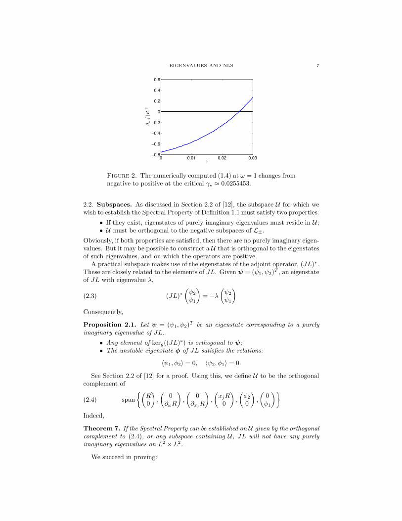
EIGENVALUES AND NLS 7
0 0.01 0.02 0.03−0.8
−0.6
−0.4
−0.2
0
0.2
0.4
0.6
γ
∂ω
∫|R
|2
Figure 2. The numerically computed (1.4) at ω = 1 changes fromnegative to positive at the critical γ? ≈ 0.0255453.
2.2. Subspaces. As discussed in Section 2.2 of [12], the subspace U for which wewish to establish the Spectral Property of Definition 1.1 must satisfy two properties:
• If they exist, eigenstates of purely imaginary eigenvalues must reside in U ;• U must be orthogonal to the negative subspaces of L±.
Obviously, if both properties are satisfied, then there are no purely imaginary eigen-values. But it may be possible to construct a U that is orthogonal to the eigenstatesof such eigenvalues, and on which the operators are positive.
A practical subspace makes use of the eigenstates of the adjoint operator, (JL)∗.These are closely related to the elements of JL. Given ψ = (ψ1, ψ2)T , an eigenstateof JL with eigenvalue λ,
(2.3) (JL)∗(ψ2
ψ1
)= −λ
(ψ2
ψ1
)
Consequently,
Proposition 2.1. Let ψ = (ψ1, ψ2)T be an eigenstate corresponding to a purelyimaginary eigenvalue of JL.
• Any element of kerg((JL)∗) is orthogonal to ψ;• The unstable eigenstate φ of JL satisfies the relations:
〈ψ1, φ2〉 = 0, 〈ψ2, φ1〉 = 0.
See Section 2.2 of [12] for a proof. Using this, we define U to be the orthogonalcomplement of
(2.4) span
{(R0
),
(0
∂ωR
),
(0
∂xjR
),
(xjR
0
),
(φ20
),
(0φ1
)}
Indeed,
Theorem 7. If the Spectral Property can be established on U given by the orthogonalcomplement to (2.4), or any subspace containing U , JL will not have any purelyimaginary eigenvalues on L2 × L2.
We succeed in proving:

8 ASAD AND SIMPSON
Theorem 8. Assume z = (f, g)T ∈ L2 × L2 satisfies the orthogonality conditions
(2.5) 〈f,R〉 = 〈f, φ2〉 = 〈g, ∂ω|ω=1R〉 = 〈g, φ1〉 = 〈f,xR〉 = 0
Then the Spectral Property holds for:
3D NLS: Provided
0.807425 < σ < 1.12092;
3D CQNLS: Provided
γ < 0.00989115;
1D NLS: Provided
2.4537956056 < σ < 6.1288520139.
For 1D and 3D NLS with power nonlinearities, we use (2.1).
3. Preliminaries
We shall prove the coercivity of B in three steps, closely following [8, 12], andomitting some details.
• In 1D, we decompose into even and odd functions and study
B+(f, f) + B−(g, g) = B(e)+ (f (e), f (e)) + B(o)+ (f (o), f (o))
+ B(e)− (g(e), g(e)) + B(o)− (g(o), g(o))(3.1)
We then show that on U , each of the four forms, B(e/o)± , is positive.Similarly, in 3D, we decompose into spherical harmonics,
B+(f, f) + B−(g, g) =
∞∑
k=0
Lk∑
l=0
B(k)+ (f (k,l), f (k,l))
+
∞∑
k=0
Lk∑
l=0
B(k)− (g(k,l), g(k,l))
(3.2)
where f (k,l) and g(k,l) are the components of f and g in harmonic k withangular component l. As L± are radially symmetric operators, they are
independent of l. Here too, we shall prove positivity of each B(k)± on U .• For each of these bilinear forms, we shall determine the codimension of
a subspace on which they are positive, called its index. This is problemspecific and can vary with the dimension and choice of nonlinearity.• Lastly, we shall show that the L2 orthogonality of f and g to U⊥ induces
orthogonality, with respect to to the bilinear form, to the negative subspacesof the form. See Section 4.1.3 for an example.
3.1. Indexes and Eigenvalues. The index of a bilinear form B on a vector spaceV is defined as
indV (B) ≡ max{k ∈ N |there exists a subspace V ⊆ Vof codimension k such that B|V is positive}
(3.3)
To compute the indexes, we rely on the following propositions:

EIGENVALUES AND NLS 9
Proposition 3.1. Let U (e) and U (o) solve the initial value problems
LU (e) = − d2
dx2u(e) + V (x)U (e) = 0, U (e)(0) = 1,
d
dxU (e)(0) = 0
LU (o) = − d2
dx2u(o) + V (x)U (o) = 0, U (o)(0) = 0,
d
dxU (o)(0) = 1
where V is even, sufficiently smooth, and |V (x)| . e−κ|x|, κ > 0, and let
B(·, ·) ≡ 〈L·, ·〉 .
Then the number of zeros of U (e) and U (o) is finite, and
indH1e(B) = number of positive roots of U (e)
= number of negative eigenvalues in H1e
indH1o(B) = number of positive roots of U (o)
= number of negative eigenvalues in H1o
H1e and H1
o are the even and odd subspaces of H1.
Proposition 3.2. Let U (k) solve the initial value problem
L(k)U (k) =
[− d2
dr2− 2
r
d
dr+ V (r) +
k2
r2
]U (k) = 0
limr→0
r−kU (k)(r) = 1, limr→0
d
dr
(r−kU (k)(r)
)= 0,
for k = 0, 1, 2, 3, . . . where V is sufficiently smooth, and |V (r)| . e−κ|r|,κ > 0, andlet
B(k)(·, ·) ≡⟨L(k)·, ·
⟩.
Then the number of zeros of U (k) is finite, and
indH1rad
(B(0)) = number of positive roots of U (0)
= number of negative eigenvalues in H1rad
indH1rad+
(B(k)) = number of positive roots of U (k), for k = 1, 2, . . .
= number of negative eigenvalues in H1rad+
The space H1rad+ is the subspace of radially symmetric H1 functions for which
∫|f |2|x|−2dx <∞.
The indexes in the different harmonics have an invaluable monotonicity propertythat permits us to restrict our attention to a finite number of harmonics:
Corollary 3.3. Fixing the potential V (r), the bilinear forms B(k) satisfy
ind(B(k+1)) ≤ ind(B(k))
The last result that we shall make use of in computing the index of a bilinearform is that it is stable to perturbation by a sufficiently localized potential:
10 ASAD AND SIMPSON
Proposition 3.4. Fixing an operator L from Propositions 3.1 or 3.2, or Corollary3.3, there exists δ0 sufficiently small such that the bilinear form, B, induced by theperturbed operator
L ≡ L− δ0e−|x|satisfies
ind(B) = ind(B)
The proofs of the preceding results are given in [12], and references therein. Asone might suspect, this is closely related to Sturm oscillation theory.
3.2. Boundary Value Problems. In the course of proving the spectral property,we will need to solve a series of problems of the form
Lu = f
for u where L is one of the above operators and f is a localized. Though thesolutions of these problems are found numerically, the invertibility of the operatorscan be rigorously justified, up to the index computation. For the index, we continueto rely on numerics.
Proposition 3.5. Let f be a smooth function, with even or odd symmetry, satis-fying the bound |f(x)| . e−κ|x| for some κ > 0. Then there exists a unique solution
u ∈ L∞(R) ∩ C2(R)
to
Lu = f.
where L is one of L±. u possesses the same symmetry as f .
Proposition 3.6. Let f be a smooth, radially symmetric, function satisfying thebound |f(r)| . e−κr for some κ > 0. Then there exists a unique solution
(1 + rk+1)u ∈ L∞(R3) ∩ C2(R3)
to
Lu = f
where L is one of L(k)± . u is radially symmetric.
While the solutions of the 3D problems decay ∝ r−1−k, the solutions of the 1Dproblems are merely bounded. Knowledge of the index of each of the operators isnecessary in proving the uniqueness of the solutions. Additionally the invertibilityof the operators is stable to perturbation:
Proposition 3.7. For sufficiently small δ0 > 0, the results of Propositions 3.5 and3.6 will also apply to
L = L − δ0e−|x|
4. Results
We are now in the position to present our results and prove Theorem 8 for eachNLS problem. From this, we can conclude Theorems 1, 2, and 3. Throughout, weshall make use of the orthogonality conditions (2.5). See Appendix A for details ofour numerical methods.
4.1. 3D Supercritical NLS.

EIGENVALUES AND NLS 11
0 1 2 3 4 5−0.5
0
0.5
1
r
U(0
)
0 1 2 3 4 5−0.5
0
0.5
1
r
Z(0
)
(a) Harmonic k = 0
0 1 2 3 4 5
0
0.5
1
r
U(1
) /r
0 1 2 3 4 50
0.5
1
r
Z(1
) /r
(b) Harmonic k = 1
0 1 2 3 4 50
0.5
1
r
U(2
) /r2
0 1 2 3 4 50.4
0.6
0.8
1
r
Z(2
) /r2
(c) Harmonic k = 2
Figure 3. Index functions for the 3D supercritical NLS equationcomputed at six values of .75 ≤ σ ≤ 1.5, inclusive.
4.1.1. Indexes.
Proposition 4.1. For .75 ≤ σ ≤ 1.5,
ind(B(0)+ ) = ind(B(0)− ) = ind(B(1)+ ) = 1
ind(B(2)+ ) = ind(B(1)− ) = 0
Proof. Examining Figures 3, we see that for six computed values of .75 ≤ σ ≤ 1.5,inclusive, we have the corresponding number of zero crossings and apply Proposition3.2. We argue by continuity that this should hold at all points in the interval. Thesewere computed using the approach described in Appendix A.1. �
Corollary 3.3 ensures positivity of the higher harmonic forms.
4.1.2. Inner Products.
Proposition 4.2. Let U(0)1 and U
(0)2 , solve
L(0)+ U
(0)1 = R(4.1a)
L(0)+ U
(0)2 = φ2(4.1b)

12 ASAD AND SIMPSON
0.8 0.9 1 1.10.5
0.6
0.7
0.8
0.9
1
1.1
1.2
σ
K(0
)1
(a)
0.8 0.9 1 1.110
−4
10−3
10−2
10−1
σ
K(0
)2
(b)
0.8 0.9 1 1.1−0.7
−0.6
−0.5
−0.4
−0.3
−0.2
−0.1
0
σ
K(0
)3
(c)
Figure 4. K(0)j as functions of σ for 3D supercritical NLS.
And define:
K(0)1 ≡
⟨L(0)+ U
(0)1 , U
(0)1
⟩,(4.2a)
K(0)2 ≡
⟨L(0)+ U
(0)2 , U
(0)2
⟩,(4.2b)
K(0)3 ≡
⟨L(0)+ U
(0)1 , U
(0)2
⟩.(4.2c)
The K(0)j have the values indicated in Figure 4. Moreover, for .8 ≤ σ ≤ 1.2,
(4.3) (K(0)1 K
(0)2 − (K
(0)3 )2)/K
(0)2 < 0
as pictured in Figure 5.
Proof. Proposition 3.6 ensures that the solutions exist. The boundary value prob-lems and inner products were computed using the techniques described in AppendixA. The (4.2) and (4.3) were then computed at 41 uniformly spaced values of σ be-tween .8 and 1.2. �

EIGENVALUES AND NLS 13
0.8 0.9 1 1.1−20
−15
−10
−5
0
σ
(K(0
)1
K(0
)2
−(K
(0)
3)2)/
K(0
)2
Figure 5. (4.3) as a function of σ for 3D supercritical NLS.
Proposition 4.3. Let Z(0)1 and Z
(0)2 , solve
L(0)− Z
(0)1 = 1
σR+ rR′(4.4a)
L(0)− Z
(0)2 = φ1(4.4b)
and define:
J(0)1 ≡
⟨L(0)− Z
(0)1 , Z
(0)1
⟩,(4.5a)
J(0)2 ≡
⟨L(0)− Z
(0)2 , Z
(0)2
⟩,(4.5b)
J(0)3 ≡
⟨L(0)− Z
(0)1 , Z
(0)2
⟩.(4.5c)
The J(0)j have the values indicated in Figure 6. Moreover there exist σ1 > .8 and
σ2 > .8 such that
J(0)1 < 0, for σ1 < σ < 1.2(4.6)
(J(0)1 J
(0)2 − (J
(0)3 )2)/J
(0)2 < 0, for σ2 < σ < 1.2(4.7)
as pictured in Figure 7, where
σ1 = 0.807699(4.8a)
σ2 = 0.807425(4.8b)
Proof. Like in the proof of Proposition 4.2, we numerically solve the boundary valueproblems at 41 uniformly spaced values of σ between .8 and 1.2. Using the rootfinding approach, discussed in Appendix A.3, we found the zero crossings, σ1 and
σ2, of J(0)1 and (??) to be at the indicated values. �
Proposition 4.4. Let U(1)1 solve
(4.9) L(1)+ U
(1)1 = rR, U
(1)1 ∈ L∞
Define
(4.10) K(1)1 ≡
⟨L(0)+ U
(1)1 , U
(1)1
⟩

14 ASAD AND SIMPSON
0.8 0.9 1 1.1−0.7
−0.6
−0.5
−0.4
−0.3
−0.2
−0.1
0
0.1
σ
J(0
)1
(a)
0.8 0.9 1 1.110
−5
10−4
10−3
10−2
σ
J(0
)2
(b)
0.8 0.9 1 1.1−0.04
−0.03
−0.02
−0.01
0
σ
J(0
)3
(c)
Figure 6. J(0)j as functions of σ for 3D supercritical NLS.
0.8 0.9 1 1.1
−3.5
−3
−2.5
−2
−1.5
−1
−0.5
0
σ
(J(0
)1
J(0
)2
−(J
(0)
3)2)/
J(0
)2
Figure 7. (4.7) as a function of σ for 3D supercritical NLS.

EIGENVALUES AND NLS 15
0.8 0.9 1 1.1−5
−4
−3
−2
−1
0
1
σ
K(1
)1
Figure 8. K(1)1 as a function of σ for 3D supercritical NLS.
There exists σ3 > .8 such that
K(1)1 < 0, for .8 ≤ σ < σ3
as pictured in Figure 8, where
(4.11) σ3 = 1.12092
Proof. This is solved in the same manner as Propositions 4.2 and 4.3. �
4.1.3. Proof of the Spectral Property. Subject to the acceptance of these computa-tions, we are now in the position to prove the spectral property for
σ2 < σ < σ3
where σ2 and σ3 are as defined by (4.8a) and (4.11). We first shall show that the
bilinear form on each harmonic, B(k)± , is positive. We first prove the case of B(0)+ .Fixing σ, for a sufficiently small δ0, in the sense of Propositions 3.4 and 3.7,
1
K(0)2
(K
(0)1 K
(0)2 − (K
(0)3 )2
)< 0.
where K(0)j is the inner product associated with the perturbed operator, L(0)
+ .Given that f is orthogonal to R and φ2, it is orthogonal to any linear combina-
tion, including
q = R− K(0)3
K(0)2
φ2
Let Q solve
(4.12) L(0)+ Q = q.
By construction,
(4.13) B(0)+ (Q, Q) =1
K(0)2
(K
(0)1 K
(0)2 − (K
(0)3 )2
)< 0.
To complete the proof of positivity, suppose Q ∈ H1rad, even thought it is not; it
decays too slowly for L2. We could decompose H1rad as
H1rad = span
{Q}⊕ span
{Q}⊥

16 ASAD AND SIMPSON
where the orthogonal decomposition is done with respect to B(0)+ . We can do this
because (4.13) implies the form is non-degenerate. Since ind(B(0)+ ) = 1, B(0)+ ≥ 0
on span{Q}⊥
. Were this not the case, it would yield a second negative direction,
independent of Q, contradicting the index computation.Given f ∈ H1
rad, f ⊥ R and f ⊥ φ2, with respect to L2 orthogonality, f is alsoL2 orthogonal to q. We might then decompose f as proposed in the precedingparagraph
f = cQ+ f⊥, B(0)+ (f⊥, Q) = 0.
If c = 0, then f = f⊥ resides in a subspace of H1rad where B(0)+ ≥ 0 , completing
the proof. We now show c = 0.Taking the L2 inner product of f and q,
0 = c⟨Q, q
⟩+⟨f⊥, q
⟩= cB(0)+ (Q, Q) +
⟨u⊥, L(0)
+ Q⟩
= cB(0)+ (Q, Q) + B(0)+ (f⊥, Q) = cB(0)+ (Q, Q) + 0.
Since we have computed B(0)+ (Q, Q) 6= 0, c = 0. Hence, L2 orthogonality to q
induces B(0)+ orthogonality to Q. Thus, f lies in the positive subspace of B(0)+ .
However, Q is not in L2. To make this argument work, one can introduce acutoff function and take an appropriate limit. We omit these details and refer thereader to [8, 12].
Positivity of B(0)− is proven similarly. In this case, we use the L2 orthogonality
of g to 1σR+ rR′ and φ1. Indeed, we construct a new Q, the solution to
L(0)− Q = 1
σR+ rR′ − J(0)3
J(0)2
φ1
However, this is only successful for σ2 < σ < 1.2.
Positivity of B(1)+ is somewhat easier, as there is no need to form a linear com-bination of elements; there is only one direction, rR, to project away from in this
harmonic. K(1)1 < 0 for all the values of .8 ≤ σ < σ3. We conclude that L2 orthog-
onality of f to rR yields positivity. Since all other forms have index zero, there isnothing to prove for them.
We have now established that
(4.14) B(z, z) ≥ 0
since each form on each harmonic is positive. It is trivial to see that
(4.15) B(z, z) ≥ δ0∫e−|x||z|2dx.
This is almost the desired expression. Consider,
(4.16) B(z, z) ≥ θ(∫|∇z|2 − |V+||f |2 − |V−||g|2dx
)+ (1− θ)δ0
∫e−|x||z|2dx
for all θ ∈ (0, 1). Both potentials satisfy the estimate |V±| . e−2σ|x|, σ > 12 , as
|x| → ∞, so taking θ sufficiently small,
(4.17) B(z, z) ≥ θ∫|∇z|2dx +
(1− θ)δ02
∫e−|x||z|2dx.

EIGENVALUES AND NLS 17
Hence,
B(z, z) &∫ (|∇z|2 + e−|x||z|2
)dx
This proves the Spectral Property from which we then immediately get Theorem1 for purely imaginary eigenvalues. As resonances in d = 3 have sufficient decay,we can also rule them out.
4.2. 3D CQNLS. In this section we prove the Spectral Property for the 3DCQNLS equation. It is quite similar to 3D NLS, though we are now concernedwith the values of γ in (1.11) for which it holds.
4.2.1. Indexes.
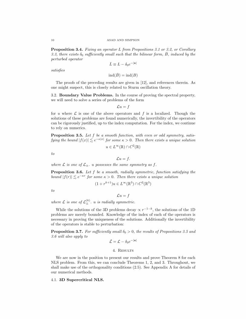
Proposition 4.5. For 0 ≤ γ ≤ .012,
indL(0)+ = indL(0)
− = indL(1)+ = 1
indL(2)+ = indL(1)
− = 0
Proof. Examining Figures 9, we see that for three computed values of 0 ≤ γ ≤.012, inclusive, we have the corresponding number of zero crossings. We argue bycontinuity that this should hold at all points in the interval. �
4.2.2. Inner Products.
Proposition 4.6. Let U(0)1 and U
(0)2 , solve
L(0)+ U
(0)1 = R(4.18a)
L(0)+ U
(0)2 = φ2(4.18b)
Define K(0)j as in (4.2). The K
(0)j have the values indicated in Figure 10. Moreover,
for 0 ≤ γ ≤ 0.012,
(4.19) (K(0)1 K
(0)2 − (K
(0)3 )2)/K
(0)1 < 0
as pictured in Figure 11.
Proof. As before, we prove this by direct computation, at twenty five values of γbetween 0 and .012, inclusive. �
Proposition 4.7. Let Z(0)1 and Z
(0)2 , solve
L(0)− Z
(0)1 = ∂ωR(4.20a)
L(0)− Z
(0)2 = φ1(4.20b)
Define J(0j as in (4.5). The J
(0)j have the values indicated in Figure 12. Moreover
there exist γ1 > 0 and σ2 > 0 such that
J(0)1 < 0, for 0 ≥ γ < γ1(4.21)
(J(0)1 J
(0)2 − (J
(0)3 )2)/J
(0)2 < 0, for 0 ≤ γ < γ2(4.22)
as pictured in Figure 13, where
γ1 = 0.00989115(4.23a)
γ2 = 0.0109065(4.23b)
18 ASAD AND SIMPSON
0 1 2 3 4 5−0.5
0
0.5
1
r
U(0
)
0 1 2 3 4 5−0.5
0
0.5
1
r
Z(0
)
(a) Harmonic k = 0
0 1 2 3 4 5
0
0.5
1
r
U(1
) /r
0 1 2 3 4 50
0.5
1
r
Z(1
) /r
(b) Harmonic k = 1
0 1 2 3 4 50
0.5
1
r
U(2
) /r2
0 1 2 3 4 50.4
0.6
0.8
1
r
Z(2
) /r2
(c) Harmonic k = 2
Figure 9. Index functions for the 3D CQNLS equation computedat three values of 0 ≤ γ ≤ .012, inclusive.
Proposition 4.8. Let U(1)1 solve
(4.24) L(1)+ U
(1)1 = rR, U
(1)1 ∈ L∞
Define K(1)1 as in (4.10). Then
K(1)1 < 0, for 0 ≤ γ0.12
as pictured in Figure 14.
4.2.3. Proof of the Spectral Property. The proof is quite similar to that of 3D NLSand we omit many of the details. For a fixed γ within the allowable range, we takeδ0 sufficiently small so as not to alter the indexes or appreciably change the innerproducts.
A notable difference is that for B(0)+ , we let Q solve
(4.25) L(0)+ Q = q = −K
(0)3
K(0)1
R+ φ2.

EIGENVALUES AND NLS 19
0 0.002 0.004 0.006 0.008 0.01 0.0120.2
0.4
0.6
0.8
1
1.2
γ
K(0
)1
(a)
0 0.002 0.004 0.006 0.008 0.01 0.012−12
−10
−8
−6
−4
−2
0
2
4
γ
K(0
)2
(b)
0 0.002 0.004 0.006 0.008 0.01 0.012−0.17
−0.16
−0.15
−0.14
−0.13
−0.12
−0.11
γ
K(0
)3
(c)
Figure 10. (4.2) as functions of γ for 3D CQNLS.
0 0.005 0.01−0.12
−0.1
−0.08
−0.06
−0.04
−0.02
0
γ
(K(0
)1
K(0
)2
−(K
(0)
3)2)/
K(0
)1
Figure 11. (4.19) as a function of γ for 3D CQNLS.

20 ASAD AND SIMPSON
0 0.002 0.004 0.006 0.008 0.01 0.012−0.2
−0.15
−0.1
−0.05
0
0.05
γ
J(0
)1
(a)
0 0.002 0.004 0.006 0.008 0.01 0.01210
−4
10−3
10−2
γ
J(0
)2
(b)
0 0.002 0.004 0.006 0.008 0.01 0.012−14
−12
−10
−8
−6
−4
−2
γ
J(0
)3
(c)
Figure 12. The J(0)j as functions of γ for 3D CQNLS.
0 0.005 0.01
−0.8
−0.6
−0.4
−0.2
0
γ
(J(0
)1
J(0
)2
−(J
(0)
3)2)/
J(0
)2
Figure 13. (J(0)1 J
(0)2 − (J
(0)3 )2)/J
(0)2 as a function of γ for 3D CQNLS.

EIGENVALUES AND NLS 21
0 0.002 0.004 0.006 0.008 0.01 0.012−1.1
−1
−0.9
−0.8
−0.7
−0.6
−0.5
γ
K(1
)1
Figure 14. K(1)1 as a function of γ for 3D CQNLS.
By construction and Proposition 4.6,
(4.26) B(0)+ (Q, Q) =1
K(0)1
(K
(0)1 K
(0)2 −
(K
(0)3
)2)< 0.
If f Is L2 orthogonal to R and φ2, then it is L2 orthogonal to any linear combination.
As before, this will induce B()+ orthogonality to Q, ensuring that B(0)+ is positive forsuch f . This holds for all 0 ≤ γ < 0.012.
Positivity of B(0)− is proven as before, except it only holds for 0 ≤ γ < γ2 due
to the results of Proposition 4.7. Positivity of B(1)+ is the same, as are the rest of
the forms, since they have index zero. This proves positivity of B on U , and thecoercivity of B on U in the form of (1.17) follows as before. This yields Theorem 2.
4.3. 1D Supercritical NLS. In contrast to the 3D problems, where we decom-posed into spherical harmonics, in 1D we decompose into even and odd functions.
4.3.1. Indexes.
Proposition 4.9. For 2.3 ≤ σ ≤ 6.3,
ind(B(e)+ ) = ind(B(e)− ) = ind(B(o)+ ) = 1, ind(B(o)− ) = 0
Proof. As before, we prove this by direct computation. The index functions appearin Figure 15. �
4.3.2. Inner Products.
Proposition 4.10. Let U(0)1 and U
(0)2 , solve
L(e)+ U
(e)1 = R(4.27a)
L(e)+ U
(e)2 = φ2(4.27b)
and define:
K(e)1 ≡
⟨L(e)+ U
(e)1 , U
(e)1
⟩,(4.28a)
K(e)2 ≡
⟨L(e)+ U
(e)2 , U
(e)2
⟩.(4.28b)

22 ASAD AND SIMPSON
0 1 2 3 4 5−10
−5
0
x
U(e
)
0 1 2 3 4 5−2
0
2
x
Z(e
)
(a) Even Functions
0 1 2 3 4 5−2
−1
0
1
x
U(o
)
0 1 2 3 4 50
2
4
x
Z(o
)
(b) Odd Functions
Figure 15. Index functions for the 1D supercritical NLS equationcomputed at five values of 2.3 ≤ σ ≤ 6.3, inclusive.
3 4 5 6−0.4
−0.3
−0.2
−0.1
0
0.1
0.2
0.3
σ
K(e
)1
(a)
3 4 5 6−5
−4
−3
−2
−1
0
σ
K(e
)2
(b)
Figure 16. The K(e)j as functions of σ for 1D supercritical NLS.
The K(e)j have the values indicated in Figure 16. Moreover,
K(e)1 < 0, for 2.3 ≤ σ < σ4
K(e)2 < 0, for 2.3 ≤ σ ≤ 6.3
where
(4.29) σ4 = 3.49928679909
Proposition 4.11. Let Z(e)1 and Z
(e)2 , solve
L(e)− Z
(e)1 = 1
σR+ xR′(4.30a)
L(e)− Z
(e)2 = φ1(4.30b)
EIGENVALUES AND NLS 23
3 4 5 6−0.7
−0.6
−0.5
−0.4
−0.3
−0.2
−0.1
0
0.1
σ
J(e
)1
(a)
3 4 5 60
0.02
0.04
0.06
0.08
0.1
0.12
0.14
0.16
σ
J(e
)2
(b)
3 4 5 6−0.15
−0.1
−0.05
0
0.05
0.1
σ
J(e
)3
(c)
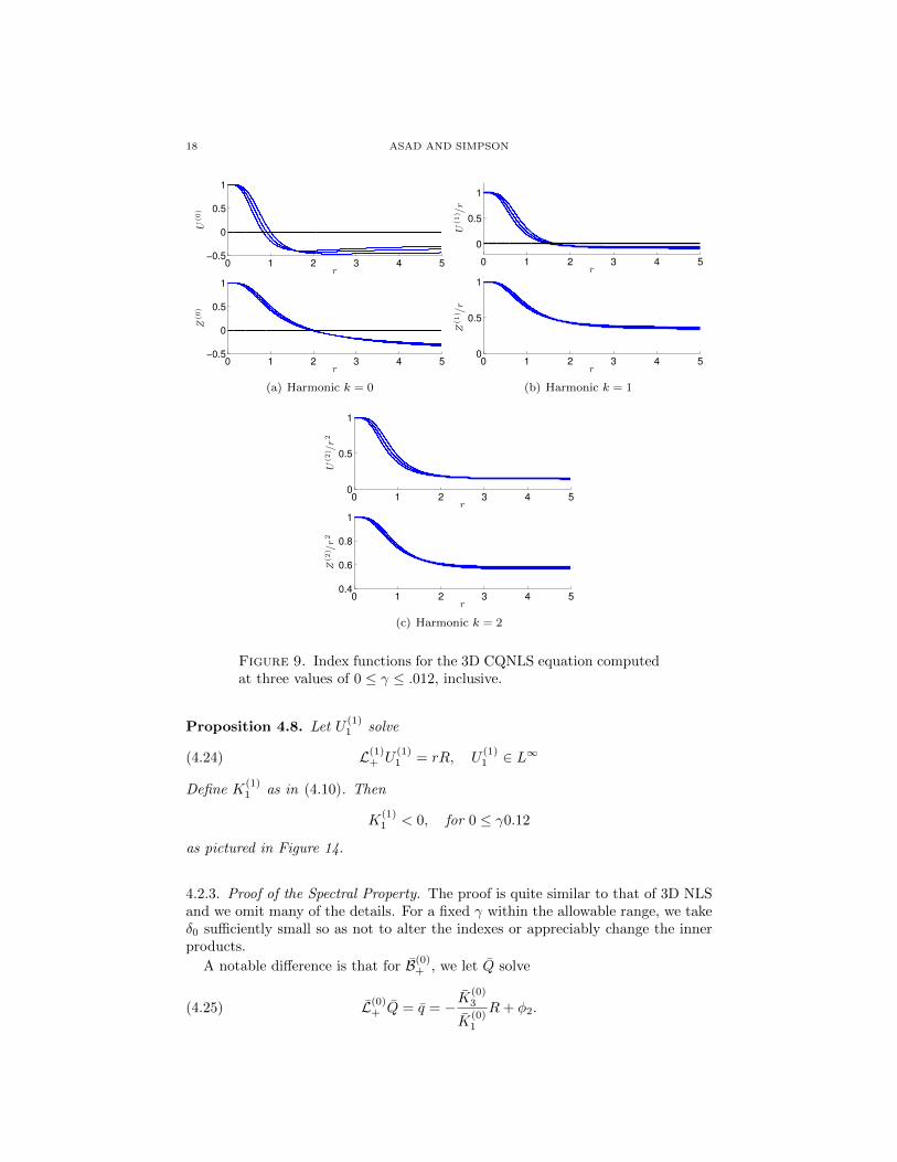
Figure 17. (4.31) as functions of σ for 1D supercritical NLS.
and define:
J(e)1 ≡
⟨L(e)− Z
(e)1 , Z
(e)1
⟩,(4.31a)
J(e)2 ≡
⟨L(e)− Z
(e)2 , Z
(e)2
⟩,(4.31b)
J(e)3 ≡
⟨L(e)− Z
(e)2 , Z
(e)1
⟩.(4.31c)
The J(0)j have the values indicated in Figure 17. Moreover,
J(e)1 < 0, for σ5 ≤ σ ≤ 6.3,(4.32a)
(J(e)1 J
(e)2 − (J
(e)3 )2)/J
(e)2 < 0, for σ6 ≤ σ ≤ 6.3,(4.32b)
where
σ5 = 2.45649878,(4.33a)
σ6 = 2.45379561.(4.33b)
Proposition 4.12. Let U(o)1 solve

24 ASAD AND SIMPSON
3 4 5 6
−1.5
−1
−0.5
0
σ
(J(e
)1
J(e
)2
−(J
(e)
3)2)/
J(e
)2
Figure 18. (4.32b) as a function of σ for 1D supercritical NLS.
3 4 5 6−1.2
−1
−0.8
−0.6
−0.4
−0.2
0
0.2
σ
K(o
)1
Figure 19. K(1)1 as a function of σ for 1D supercritical NLS.
(4.34) L(o)+ U
(o)1 = xR
and define
(4.35) K(o)1 ≡
⟨L(o)+ U
(o)1 , U
(o)1
⟩.
K(o)1 has the values indicated in Figure 19. Moreover,
K(o)1 < 0, for 2.3 ≤ σ ≤ σ7
where
(4.36) σ7 = 6.1288520139
4.3.3. Proof of the Spectral Property. To prove the spectral property in this case, we
can use the orthogonality of f to φ2 to induce positivity of B(e)+ for all 2.3 ≤ σ ≤ 6.3,
via Proposition 4.10. For B(e)− , L2 orthogonality to 1σR + xR′ and φ1 induces
positivity for σ6 < σ ≤ 6.3 through Proposition 4.11. Finally, Proposition 4.12
yields positivity of B(o)+ for 2.3 ≤ σ < σ7.

EIGENVALUES AND NLS 25
5. Discussion
We have successfully proven there are no purely imaginary eigenvalues, bothin the spectral gap and embedded in the essential spectrum, for a collection of aorbitally unstable solitary wave solutions of NLS. However, there is still much to bedone. First, the range of orbitally unstable solitary waves has not been exhausted.We know there are no purely imaginary eigenvalues for σ > 2 in the 1D NLSequation, and we anticipate that there are none for σ > 2/3 in 3D. We expectsimilar results for the entire unstable branch of CQNLS. Second, we have shownthat the threshold found in [6], given by (1.10), is suboptimal; our range, (1.12), islarger, but it too is likely suboptimal.
This work also raises questions of what is satisfactory for a rigorous proof. Werelied on the computer in the following steps:
• Computing the solitary waves for the 3D, a nonlinear boundary value prob-lem on an unbounded domain;• Computing a finite number of index functions, linear initial value problems
on unbounded domains;• Solving a finite collection of linear elliptic problems on unbounded domains;• Computing inner products on an unbounded intervals.
To deal with these obstacles we truncated the intervals to [0, rmax] ([0, xmax] in 1D),and introduced a finite number of discretization points within the intervals. Evenwith these computations, we have only established the results for isolated valuesof σ or γ; we argue by continuity that the results should extend to continuousintervals.
However, we are able to produce a variety of consistency and a posteriori checks,such as verifying that the artificial boundary conditions are being satisfied suffi-ciently well. Despite our confidence in our computations, it would still be desirableto avoid the use of the computer. Indeed, an alternative method may permit us tomove beyond the seemingly artificial restrictions on σ and γ of our results.

26 ASAD AND SIMPSON
Appendix A. Numerical Methods
The codes used to produce the results appearing in this work are available athttp://www.math.toronto.edu/simpson/files/spec_prop_asad_simpson_code.
zip for examination, verification, and experimentation.The numerical methods we use are the same as those used in [12], and separately
in Simpson & Zwiers, [20]. For the 3D problems, we use the Fortran 90/95 basedboundary value problem solver of Shampine, Muir, & Xu, [19]. For the 1D problems,we found it sufficient to use the closely related bvp4c routine in Matlab , [17,18].These algorithms require us to specify the problems as first order systems of theform
d
dry = 1
rSy + f(r,y)
where S is a constant matrix and f contains all non-singular terms, both linear andnonlinear.
This automatically accommodates problems involving r−1 type singularities atthe origin, as found in the equation for the 3D solitons and the k = 0 harmonicboundary value problems. For higher harmonics, we use a point transformationW (r) = rkW (r) to transform
[− d2
dr2− d− 1
r
d
dr+k(k + d− 2)
r2
]W ⇒ rk
[− d2
dr2− d− 1 + 2k
r
d
dr
]W .
A.1. Index Functions. For the 3D problems, we computed the index functionson the domain [0, 200] with a tolerance setting of 10−13. The 1D problems werecomputed on the domain [0, 100] with absolute and relative tolerances of 10−13.While Figures 3, 9, and 15 show the indicated numbers of roots, they obviously donot prove that there is no root at some larger value of x or r.
To mitigate this uncertainly, there are two things we can check. First, we canexamine the solution on a much larger domain. A more systematic approach isto note that since the potentials are highly localized, asymptotically, the indexfunctions satisfy the estimates
U (k)(r) ≈ C(k)0 rk + C
(k)1 r2−d−k(A.1a)
Z(k)(r) ≈ D(k)0 rk +D
(k)1 r2−d−k(A.1b)
where C(k)j and D
(k)j are constants. Estimating these constants, and seeing that
they have the correct signs and magnitudes, indicates that there cannot be further
roots. For example, in Figure 20, we see that C(0)0 ≈ −0.3668 and C
(0)1 ≈ −0.2393.
The only root of
−0.3668− 0.2393/r
is near −0.65. Thus, there should be no zeros in the “far field”. Similar analysis
works for the D(0)j constants.
A.2. Boundary Value Problems & Artificial Boundary Conditions. Sincethis algorithm requires us to compute on a finite domain, [0, rmax], we must in-troduce artificial boundary conditions at rmax. These are discussed in the above

EIGENVALUES AND NLS 27
0 1 2 3 4 5−0.5
0
0.5
1
r
U(0
)
0 1 2 3 4 5−0.5
0
0.5
1
r
Z(0
)
50 100 150 200−0.3668
−0.3668
−0.3668
−0.3668
r
C(0
)0
50 100 150 200−0.2393
−0.2393
−0.2393
−0.2393
r
C(0
)1
50 100 150 200−2
−1
0
1
r
D(0
)0
50 100 150 2001.0668
1.0668
1.0668
1.0668
1.0668
r
D(0
)1
Figure 20. The index functions and the asymptotic constants forthe γ = .01 case of CQNLS in harmonic k = 0.
20 40 60 80 100
10−30
10−20
10−10
r
RU
(0)1
U(0)2
φ1
φ2
Figure 21. Verification of the artificial boundary conditions forthe soliton, R, the eigenstate, φ, and the solutions of the boundary
value problems U(0)j for the γ = 0.01 case of CQNLS.
references, but include
R(rmax) +rmax
1 + rmaxR′(rmax) = 0
∂ω|ω=1R(rmax) + ∂ω|ω=1R′(rmax) = 0
for the 3D problems. Again, additional details are given in [12, 20]. An exampleof an a posteriori check of these being satisfied is given in Figure 21, which in-cludes computations of the soliton, the unstable eigenstate, and the solutions ofthe boundary value problems for Proposition 4.6.
The boundary value problems were solved on the domain [0, 100] in all cases. Forthe 3D problems, the tolerance was set at 10−12. for the 1D problems, the absolutetolerance was 10−8 and relative tolerance was 10−10.
A.3. Root Finding. To compute roots of the inner products, or combinations ofthem, we wrap our routines within the fzero routine, with default settings, ofMatlab ; we define a function that, for a given value of σ or γ, returns the innerproduct, and pass this to fzero. We found this could provide approximately six

28 ASAD AND SIMPSON
0 2 4 6 8
x 10−7
−6
−4
−2
0
2
4
6x 10
−6
σ − 0.8076980
J(0
)1
Figure 22. Zooming in on the root of J(0)1 inner product of the
3D NLS equation, the solution is appears piecewise constant. Thisis a closeup of Figure 6(a).
digits of accuracy in our 3D computations, notably for the bounds (1.12) and (1.13),while for the 1D computations, we were able to get eleven digits.
There appears to be a loss of sensitivity to the input σ or γ for the 3D problems.An example of this appears in Figure 22, where we see that for a range of σ values
near the root, J(0)1 is piecewise constant. Refinements to our approach, with higher
order corrections to the artificial boundary conditions, may improve the accuracy.

EIGENVALUES AND NLS 29
References
[1] V. S. Buslaev and G. S. Perel′man. On the stability of solitary waves for nonlinear Schrodingerequations. In Nonlinear evolution equations, volume 164 of Amer. Math. Soc. Transl. Ser. 2,
pages 75–98. Amer. Math. Soc., Providence, RI, 1995.
[2] V. S. Buslaev and C. Sulem. On asymptotic stability of solitary waves for nonlinearschrodinger equations. Ann. Inst. H. Poincare Anal. Non Lineaire, 20(3):419–475, 2003.
[3] S. Cuccagna. On asymptotic stability of ground states of NLS. Rev. Math. Phys., 15(8):877–
903, 2003.[4] S. Cuccagna and D. Pelinovsky. Bifurcations from the endpoints of the essential spectrum in
the linearized nonlinear Schrodinger problem. J. Math. Phys., 46(5):053520, 15, 2005.[5] S. Cuccagna, D. Pelinovsky, and V. Vougalter. Spectra of positive and negative energies in
the linearized NLS problem. Comm. Pure Appl. Math., 58(1):1–29, 2005.
[6] L. Demanet and W. Schlag. Numerical verification of a gap condition for a linearized nonlinearSchrodinger equation. Nonlinearity, pages 829–852, 2006.
[7] M. B. Erdogan and W. Schlag. Dispersive estimates for schrodinger operators in the presence
of a resonance and/or an eigenvalue at zero energy in dimension three. ii. Journal d’AnalyseMathematique, 99:199–248, 2006.
[8] G. Fibich, F. Merle, and P. Raphael. Proof of a Spectral Property related to the singular
formation for the L2 critical nonlinear Schrodinger equation. Physica D, 220:1–13, 2006.[9] M. Grillakis, J. Shatah, and W. Strauss. Stability theory of solitary waves in the presence of
symmetry. i. J Funct Anal, 74(1):160–197, 1987.
[10] M. Grillakis, J. Shatah, and W. Strauss. Stability theory of solitary waves in the presence ofsymmetry. ii. J Funct Anal, 94(2):308–348, 1990.
[11] J. Krieger and W. Schlag. Stable manifolds for all monic supercritical focusing nonlinear
Schrodinger equations in one dimension. J. Amer. Math. Soc., 19(4):815–920, 2006.[12] J. L. Marzuola and G. Simpson. Spectral analysis for matrix hamiltonian operators. Nonlin-
earity, 24:389–429, 2011.[13] F. Merle and P. Raphael. The blow-up dynamic and upper bound on the blow-up rate for
critical nonlinear Schrodinger equation. Annals of Mathematics, pages 157–222, 2005.
[14] G. Perelman. Personal communication to Wilhelm Schlag.[15] I. Rodnianski, W. Schlag, and A. Soffer. Asymptotic stability of N -soliton states of NLS.
Preprint, 2003.
[16] W. Schlag. Stable manifolds for an orbitally unstable nonlinear schrodinger equation. Ann.of Math. (2), 169(1):139–227, 2009.
[17] L. Shampine. Singular boundary value problems for ODEs. Applied Mathematics and Com-
putation, 138(1):99–112, 2003.[18] L. Shampine, I. Gladwell, and S. Thompson. Solving ODEs with MATLAB. Cambridge Uni-
versity Press, 2003.
[19] L. Shampine, P. Muir, and H. Xu. A User-Friendly Fortran BVP Solver. JNAIAM, 1(2):201–217, 2006.
[20] G. Simpson and I. Zwiers. Vortex collapse for the l2-critical nonlinear schrodinger equation.arXiv, math.AP, Oct 2010. 36 pages, 10 figures.
[21] C. Sulem and P. Sulem. The Nonlinear Schrodinger Equation: Self-Focusing and WaveCollapse. Springer, 1999.
[22] M. I. Weinstein. Modulational stability of ground states of nonlinear schrodinger equations.
SIAM Journal on Mathematical Analysis, 16:472, 1985.
[23] M. I. Weinstein. Lyapunov stability of ground states of nonlinear dispersive evolution equa-tions. Communications on Pure and Applied Mathematics, pages 51–68, 1986.
E-mail address: [email protected]
Department of Mathematics, University of Toronto, Toronto, Canada
E-mail address: [email protected]
Department of Mathematics, University of Toronto, Toronto, Canada