elements of quantum computing and qubits

Elements of Quantum Computing

and Qubits

Mattia Checchin

QuarkNet Workshop, Fermilab, Batavia IL, USA

18 – 20 July 2018

Outline

✱Introduction

✱What is a qubit?

✱How does a qubit work?

✱Quantum state manipulation

✱Qubit readout

✱Quantum computing R&D at Fermilab

✱Conclusions

Mattia Checchin | QuarkNet Workshop, Fermilab, Batavia IL, USA2

Outline

✱Introduction

✱What is a qubit?



✱Qubit readout


✱Conclusions


I - What is a quantum computer?

✱ A quantum computer is a computation framework based on quantum

mechanics phenomena:

– Superposition of states

– Entanglement

✱ The computational building block of quantum computers are so-called

qubits (quantum bits)

✱ Any qubit is a quantum system defined by ground ȁ 𝟎 and excited ȁ 𝟏states

✱ A quantum computer would have many qubits coupled together, along

with input control lines and output measurement lines

✱ The first step in operating a quantum computer would be to prepare all the

qubits in the ground state:

ȁ 𝜳(𝟎) = ȁ 𝟎 ȁ 𝟎 ȁ 𝟎 ȁ 𝟎 ȁ 𝟎 … ȁ 𝟎 ȁ 𝟎 ȁ 𝟎 ȁ 𝟎 ȁ 𝟎


II - What is a quantum computer?

✱ A quantum computer performs “gate operations” by applying a

perturbation (force, current, voltage, magnetic field, photon, rf drive...) to

the qubits

✱ Any gate outcome is a transformation of the qubit state which will evolve

from the ground state ȁ 𝜳(𝟎) to the state ȁ 𝜳(𝒕) in a time 𝑡

✱ The perturbation lasts for a specified time and the time-evolution of the

state is completely deterministic! With the right perturbation you could flip

any qubit state from 0 to 1 (NOT) or perform other operations....

✱ After a series of gates, each qubit may be left in 0, or in 1, or in an

entangled quantum superposition of 0 and 1... both 0 and 1

simultaneously and correlated with the state of other qubits ... a very non-

classical result

✱ The state of each qubit is then measured, producing a result of the

calculation: a string of ȁ 𝟎 and ȁ 𝟏 . The result is probabilistic!


What’s the deal?

✱ Let’s assume a 2 bit register. All the possible states the system can access is:

✱ Let’s now assume a 2 qubit quantum register. Since the qubit can be 0 and 1

simultaneously, the quantum register is defined by the superposition of states

ฬ 01

01

(as if we had 4 PC working in parallel). All the possible states the system

can access is:


𝑆𝑡𝑎𝑡𝑒 =01

01

= ൞

00011011

⇒ 𝟐𝟐 = 𝟒 possible states

ȁ 𝛹 = 𝑎1 ฬ 01

01

+ 𝑎2 ฬ 01

01

+ 𝑎3 ฬ 01

01

+ 𝑎4 ฬ 01

01

; σ𝑖𝑛 𝑎𝑖

2 = 1

𝑎1

ȁ 00ȁ 01ȁ 10ȁ 11

𝑎2

ȁ 00ȁ 01ȁ 10ȁ 11

𝑎3

ȁ 00ȁ 01ȁ 10ȁ 11

𝑎4

ȁ 00ȁ 01ȁ 10ȁ 11

⇒ 𝟐𝟐𝟐= 𝟏𝟔 possible states!

✱ A quantum computer with n qubits could then access to a total

of 𝟐𝟐𝒏

superposition states and entangled states ... compared to

𝟐𝒏 states for a classical computer with an n-bit memory

✱ Huge number of accessible states would allow a quantum computer to solve certain problems that are otherwise intractable (e.g. factorization of big numbers)

Quantum computer have much more available states!


Outline

✱Introduction

✱What is a qubit?



✱Qubit readout


✱Conclusions


What is a qubit?

✱ Classical bit:

– Based on transistor

– Described by 2 possible states:

• 0 – “off”

• 1 – “on”

✱ Quantum bit:

– ANY two energy levels quantum system

– Described by the linear combination (ȁ Ψ ) of 2 quantum states

• ȁ 𝛹 = 𝛼ȁ 0 + 𝛽ȁ 1

– ȁ 0 – ground state

– ȁ 1 – excited state

– 𝛼 2 and 𝛽 2 probabilities that the qubit is in the state ȁ 0 or ȁ 1 respectively


✱ Nature already provide us with qubits: ATOMS!

✱ I can select an electronic transition between two orbitals and

define a two level system

✱ HOWEVER, atoms are difficult to manipulate, electronic

transitions are in the range of visible/UV spectrum, etc…

Atoms: natural qubits


n=1

n=2

n=3

ℏ𝜔

+Zeȁ 1

ȁ 0

ȁ 2

ℏ𝜔

Resonators: not yet qubits

✱ If we take a single resonant

mode of any resonator, it looks

like a harmonic oscillator

✱ HOWEVER, the energy

separation between levels is

even ⇒ I cannot select a

specific transition


ȁ 1

ȁ 0

ȁ 2∆𝐸

∆𝐸

✱ As of now the most adopted

✱ Based on Josephson junctions:

non-linear inductors

✱ Behaves as an anharmonic LC

resonator, transitions can be

tuned in the microwave spectra

⇒ a perfect artificial atom!

Superconducting qubits


ȁ 1

ȁ 0

ȁ 2 ∆𝐸1→2

∆𝐸0→1

SC Insulator SC

Schematics of a Josephson junction

∆𝐸0→1≠ ∆𝐸1→2

Typical layout of a quantum computation experiment


✱ Very low temperature (milli-Kelvin) are mandatory to avoid thermal excitation of the qubit!

𝜅𝐵𝑇 < ℏ𝜔

Dilution refrigerator

Outline

✱Introduction

✱What is a qubit?



✱Qubit readout


✱Conclusions


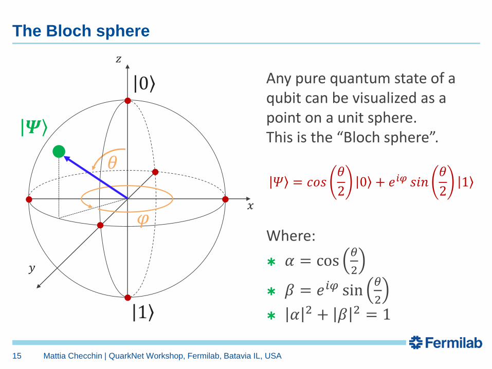
Any pure quantum state of a qubit can be visualized as a point on a unit sphere. This is the “Bloch sphere”.

Where:

✱ 𝛼 = cos𝜃

2

✱ 𝛽 = 𝑒𝑖𝜑 sin𝜃

2

✱ 𝛼 2 + 𝛽 2 = 1

The Bloch sphere


ȁ 1

ȁ 0

𝑧

𝑦

𝑥

𝜃

𝜑

ȁ 𝜳

ȁ 𝛹 = 𝑐𝑜𝑠𝜃

2ȁ 0 + 𝑒𝑖𝜑 𝑠𝑖𝑛

𝜃

2ȁ 1

✱ 𝜃 = 0

The Bloch sphere: example 1


ȁ 1

ȁ 𝟎

𝑧

𝑦

𝑥

ȁ Ψ = cos𝜃

2ȁ 0 + 𝑒𝑖𝜑 sin

𝜃

2ȁ 1

= cos 0 ȁ 0 + 𝑒𝑖𝜑 sin 0 ȁ 1

= ȁ 0

✱ 𝜃 = π



ȁ 𝟏

ȁ 0

𝑧

𝑦

𝑥

ȁ Ψ = cos𝜃


𝜃

2ȁ 1

= cosπ


π

2ȁ 1

= 𝑒𝑖𝜑ȁ 1𝜃 = 𝜋

✱ 𝜃 = Τ𝜋 2, 𝜑 = Τ𝜋 2



ȁ 1

ȁ 0

𝑧

𝑦

𝑥

ȁ Ψ = cos𝜃


𝜃

2ȁ 1

= cosπ

4ȁ 0 + 𝑒𝑖

π2 sin

π

4ȁ 1

=ȁ 0 + 𝑖 ȁ 1

2

ȁ 𝟎 + 𝒊 ȁ 𝟏

𝟐

𝜑 = Τ𝜋 2

𝜃 = Τ𝜋 2

Outline

✱Introduction

✱What is a qubit?



✱Qubit readout


✱Conclusions


I - Qubit driven at the transition frequency


ȁ 0

ȁ 1

ȁ 0

ȁ 1

ȁ 0

ȁ 1

𝛼 2 = 1

𝛽 2 = 0

𝛼 2 = 0

𝛽 2 = 1

𝛼 2 = 1

𝛽 2 = 0

ℏ𝜔01 ℏ𝜔01 ℏ𝜔01

Ground state

✱ Let’s assume a qubit with transition energy ∆𝐸

✱ The qubit is at its ground state ȁ 0✱ Let’s apply a EM perturbation with frequency 𝜔01 = ∆𝐸/ℏ✱ The qubit state will evolve with time:

ȁ Ψ 𝑡 = 𝛼 𝑡 ȁ 0 + 𝛽 𝑡 ȁ 1

II - Qubit driven at the transition frequency


ȁ 0

ȁ 1

ȁ 0

ȁ 1

ȁ 0

ȁ 1

𝛼 2 = 1

𝛽 2 = 0

𝛼 2 = 0

𝛽 2 = 1

𝛼 2 = 1

𝛽 2 = 0


Absorption



ȁ Ψ 𝑡 = 𝛼 𝑡 ȁ 0 + 𝛽 𝑡 ȁ 1

III - Qubit driven at the transition frequency


ȁ 0

ȁ 1

ȁ 0

ȁ 1

ȁ 0

ȁ 1

𝛼 2 = 1

𝛽 2 = 0

𝛼 2 = 0

𝛽 2 = 1

𝛼 2 = 1

𝛽 2 = 0


Stimulated emission



ȁ Ψ 𝑡 = 𝛼 𝑡 ȁ 0 + 𝛽 𝑡 ȁ 1



ȁ Ψ 𝑡 = 𝛼 𝑡 ȁ 0 + 𝛽 𝑡 ȁ 1

IV - Qubit driven at the transition frequency


ȁ 0

ȁ 1

ȁ 0

ȁ 1

ȁ 0

ȁ 1

𝛼 2 = 1

𝛽 2 = 0

𝛼 2 = 0

𝛽 2 = 1

𝛼 2 = 1

𝛽 2 = 0


✱ ȁ Ψ 𝑡 oscillates between ȁ 0 and ȁ 1 with frequency Ω, the Rabi frequency

✱ ȁ Ψ 𝑡 precesses around 𝑧 with frequency 𝜔01

✱ By controlling pulses length and time delays any state is accessible

Driven qubit: quantum state evolution


𝑧

𝑦

𝑥

Ω

𝜔01

ȁ 1

ȁ 0

ȁ Ψ 𝑡 = cosΩ𝑡

2ȁ 0 + 𝑒𝑖𝜔01𝑡 sin

Ω𝑡

2ȁ 1

✱ Let’s drive the qubit with frequency 𝜔01 = ∆𝐸/ℏ✱ The qubit state will be: 𝜃 𝜑 𝜃

Example: 𝝅-pulse (NOT)


𝑧

𝑦

𝑥

𝛼 𝑡 = cosΩ𝑡

2

𝛽 𝑡 = 𝑒𝑖𝜔01𝑡 sinΩ𝑡

2

ȁ 1

ȁ 0

𝜃 = 𝜋

✱ 𝜋-pulse is the qubit equivalent of a classical NOT operation: ȁ 0 → ȁ 1

2𝜋/𝜔01

2𝜋/Ω

Drive signal

Occupationprobability

𝑡 = Τ2𝜋 Ω

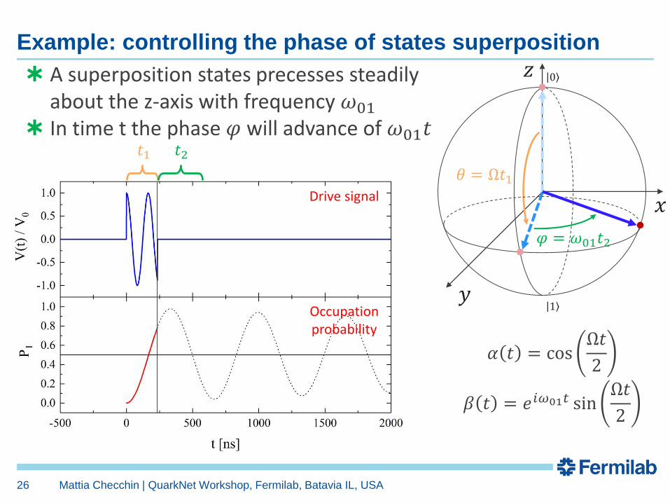
Example: controlling the phase of states superposition


𝑧

𝑦

𝑥

𝛼 𝑡 = cosΩ𝑡

2

𝛽 𝑡 = 𝑒𝑖𝜔01𝑡 sinΩ𝑡

2

ȁ 1

ȁ 0

𝜃 = Ω𝑡1

✱ A superposition states precesses steadily about the z-axis with frequency 𝜔01

✱ In time t the phase 𝜑 will advance of 𝜔01𝑡

Drive signal

Occupationprobability

𝜑 = 𝜔01𝑡2

𝑡1 𝑡2

Quantum information is stored in amplitude and phase…but it can be lost!

• Energy relaxation

• Dephasing

Qubit decoherence mechanisms


𝑧

𝑦

𝑥

ȁ 1

ȁ 0

✱ Due to finite relaxation time 𝑇1 of the first

excited state- Need qubits that do not lose energy quickly...

must not radiate electromagnetic energy or

couple to other quantum systems

𝑧

𝑦

𝑥

ȁ 1

ȁ 0

✱ Random fluctuations in qubit energy level

spacing causes random fluctuations in phase 𝜑of superposition states - Phase information lost on time scale 𝑇𝜑- Design qubit so it can’t couple to anything

Decoherence time: 1

𝑇2=

1

2𝑇1+

1

𝑇𝜑

Outline

✱Introduction

✱What is a qubit?



✱Qubit readout


✱Conclusions


The Schrödinger cat problem


The cat is deadSuperposition of states The cat is alive

Measurement

✱ The observation of a quantum state (measurement) collapses the system state in one of its eigen-states

✱We loose info on superposition of states⇒ bad for quantum computation!

Quantum non-demolition measurements

✱ Resonator coupled to a qubit

✱ Probing the perturbation on the resonator induced by the

state of the qubit


3D architecture 2D architecture

Resonator

Qubit

Yale

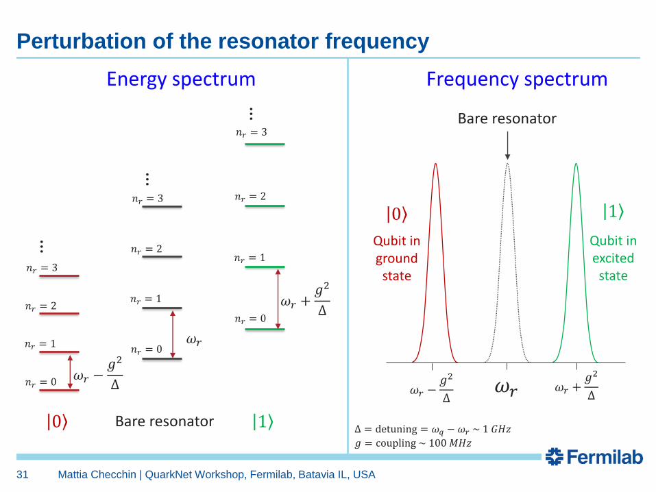
Perturbation of the resonator frequency


𝜔𝑟

ȁ 1ȁ 0

Qubit in excited state

Qubit in ground state

ȁ 1ȁ 0 Bare resonator

Bare resonator

𝜔𝑟

Energy spectrum

𝜔𝑟 −𝑔2

Δ

𝜔𝑟 +𝑔2

Δ

Frequency spectrum

𝜔𝑟 −𝑔2

Δ𝜔𝑟 +

𝑔2

Δ

…

𝑛𝑟 = 0

𝑛𝑟 = 1

𝑛𝑟 = 2

𝑛𝑟 = 3

…

𝑛𝑟 = 0

𝑛𝑟 = 1

𝑛𝑟 = 2

𝑛𝑟 = 3

…

𝑛𝑟 = 0

𝑛𝑟 = 1

𝑛𝑟 = 2

𝑛𝑟 = 3

Δ = detuning = 𝜔𝑞 − 𝜔𝑟 ~ 1 𝐺𝐻𝑧

𝑔 = coupling ~ 100 𝑀𝐻𝑧

Outline

✱Introduction

✱What is a qubit?



✱Qubit readout


✱Conclusions


SRF Cavities: from accelerators to quantum computing


+

SRF cavities typically used to accelerate charged particles because:

✱ Very high Q-factors:𝑄0 > 1010 (low power dissipation)

✱ Very high accelerating voltages: 𝑉𝑎𝑐𝑐 ≅ 40,000,000 𝑉 in 1 𝑚

HOWEVER,high Q-factor resonators

are also needed to increase coherence time in quantum computers!

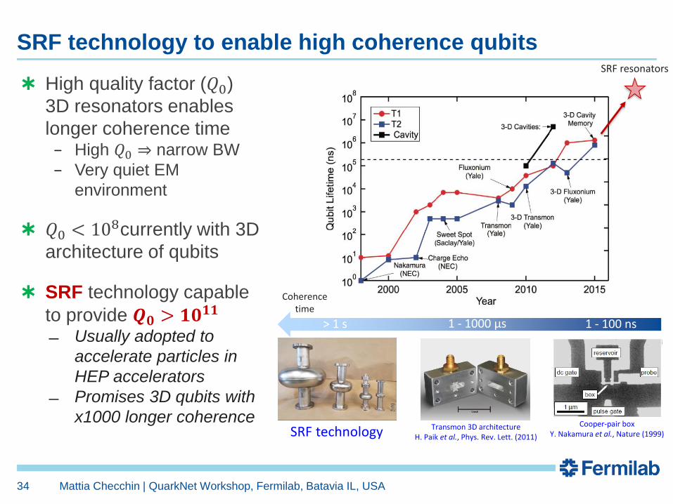
SRF technology to enable high coherence qubits


Transmon 3D architectureH. Paik et al., Phys. Rev. Lett. (2011)

Cooper-pair boxY. Nakamura et al., Nature (1999)

✱ High quality factor (𝑄0)

3D resonators enables

longer coherence time− High 𝑄0 ⇒ narrow BW

− Very quiet EM

environment

✱ 𝑄0 < 108currently with 3D

architecture of qubits

✱ SRF technology capable

to provide 𝑸𝟎 > 𝟏𝟎𝟏𝟏

Usually adopted to

accelerate particles in

HEP accelerators

Promises 3D qubits with

x1000 longer coherenceSRF technology

> 1 s 1 - 1000 μs 1 - 100 ns

Coherencetime

SRF resonators

First measurements towards quantum regime


Qu

alit

y F

acto

r

Eacc (MV/m)

0.001 0.01 0.1 1 10

1x1010

3x1010

5x1010

7x1010

9x1010

Saturation of the

Q decrease

Fit to TLS model

Ec = 0.1 MV/m

b = 0.19

CWSS RBW=10 kHzSS RBW=30 Hz

T=1.5K

Now measured down to <N> ~ 1000 photons

Good news: low field Q saturates at Q > 3 x 1010

1.3 GHz

A. Romanenko and D. I. Schuster, Phys . Rev. Lett. 119, 264801 (2017)

New quantum computing lab at Fermilab


…some pics…

Outline

✱Introduction

✱What is a qubit?



✱Qubit readout


✱Conclusions


Many universities and silicon valley industries did themain breakthroughs in quantum computation…

…Fermilab is new in the QIS scene, but seeks tobecome competitive in this field by providingextensive knowhow on high Q-factor SRF resonators

Quantum Information Science (QIS) and Fermilab


…and others…

Conclusions

✱ The last decade has seen remarkable progress towards building a

quantum computer

✱ In superconducting qubits, the lifetimes have improved by orders of

magnitude and the longest lifetimes exceed 1 millisecond

✱ Superconducting qubits and trapped ion qubits have advanced to

the point where they can be scaled up to many more qubits

✱ Things should get “interesting” at the 30 to 100 qubit level

✱ Key research issues:

– Eliminating/reducing sources of relaxation and dephasing

– High-fidelity gates and read out

– Implementing error correction

– Controllable coupling of qubits

– Reaching small, medium and large scale integration


elements of quantum computing and qubits

Documents