elements of hilbert space and operator theory · chapter 1 reviews vector spaces: bases, subspaces,...

Bo Li

Department of Mathematics

University of California, San Diego

Elements of Hilbert Space and

Operator Theory

with Application to Integral Equations

May 30, 2005

Preface

These lecture notes present elements of Hilbert space and the theory of linearoperators on Hilbert space, and their application to integral equations.

Chapter 1 reviews vector spaces: bases, subspaces, and linear transforms.Chapter 2 covers the basics of Hilbert space. It includes the concept of Ba-nach space and Hilbert space, orthogonality, complete orthogonal bases, andRiesz representation. Chapter 3 presents the core theory of linear operators onHilbert space, in particular, the spectral theory of linear compact operatorsand Fredholm Alternatives. Chapter 4 is the application to integral equations.Some supplemental materials are collected in Appendicies.

The prerequisite for these lecture notes is calculus. Occasionally, advancedknowledges such as the Lebesgue measure and Lebesgue integration are usedin the notes. The lack of such knowledge, though, will not prevent readersfrom grasping the essence of the main subjects.

The presentation in these notes is kept as simple, concise, and self-completeas possible. Many examples are given, some of them with great details. Ex-ercise problems for practice and references for further reading are included ineach chapter.

The symbol ⊓⊔ is used to indicate the end of a proof.These lecture notes can be used as a text or supplemental material for

various kinds of undergraduate or beginning graduate courses for students ofmathematics, science, and engineering.

Bo LiSpring, 2005

Contents

1 Vector Spaces . . . . . . . . . . . . . . . . . . . . . . . . . . . . . . . . . . . . . . . . . . . . . 11.1 Definition . . . . . . . . . . . . . . . . . . . . . . . . . . . . . . . . . . . . . . . . . . . . . . 11.2 Linear Dependence . . . . . . . . . . . . . . . . . . . . . . . . . . . . . . . . . . . . . . 51.3 Bases and Dimension . . . . . . . . . . . . . . . . . . . . . . . . . . . . . . . . . . . . 91.4 Subspaces . . . . . . . . . . . . . . . . . . . . . . . . . . . . . . . . . . . . . . . . . . . . . . 171.5 Linear Transforms . . . . . . . . . . . . . . . . . . . . . . . . . . . . . . . . . . . . . . . 17Exercises . . . . . . . . . . . . . . . . . . . . . . . . . . . . . . . . . . . . . . . . . . . . . . . . . . . 17References . . . . . . . . . . . . . . . . . . . . . . . . . . . . . . . . . . . . . . . . . . . . . . . . . . 18

2 Hilbert Spaces . . . . . . . . . . . . . . . . . . . . . . . . . . . . . . . . . . . . . . . . . . . . . 192.1 Inner Products . . . . . . . . . . . . . . . . . . . . . . . . . . . . . . . . . . . . . . . . . . 192.2 Normed Vector Spaces . . . . . . . . . . . . . . . . . . . . . . . . . . . . . . . . . . . 202.3 Hilbert Spaces . . . . . . . . . . . . . . . . . . . . . . . . . . . . . . . . . . . . . . . . . . 202.4 Orthogonality . . . . . . . . . . . . . . . . . . . . . . . . . . . . . . . . . . . . . . . . . . . 202.5 Complete Orthogonal Bases . . . . . . . . . . . . . . . . . . . . . . . . . . . . . . . 202.6 Riesz Representation . . . . . . . . . . . . . . . . . . . . . . . . . . . . . . . . . . . . . 20Exercises . . . . . . . . . . . . . . . . . . . . . . . . . . . . . . . . . . . . . . . . . . . . . . . . . . . 20References . . . . . . . . . . . . . . . . . . . . . . . . . . . . . . . . . . . . . . . . . . . . . . . . . . 20

3 Operator Theory . . . . . . . . . . . . . . . . . . . . . . . . . . . . . . . . . . . . . . . . . . 213.1 Bounded Linear Operators . . . . . . . . . . . . . . . . . . . . . . . . . . . . . . . . 213.2 Self-Adjoint Operators . . . . . . . . . . . . . . . . . . . . . . . . . . . . . . . . . . . 313.3 Compact Operators . . . . . . . . . . . . . . . . . . . . . . . . . . . . . . . . . . . . . . 31Exercises . . . . . . . . . . . . . . . . . . . . . . . . . . . . . . . . . . . . . . . . . . . . . . . . . . . 32References . . . . . . . . . . . . . . . . . . . . . . . . . . . . . . . . . . . . . . . . . . . . . . . . . . 32

4 Integral Equations . . . . . . . . . . . . . . . . . . . . . . . . . . . . . . . . . . . . . . . . . 334.1 Examples and Classification of Integral Equatons . . . . . . . . . . . . 334.2 Integral Equations of the Second Kind: Successive Iterations . . 334.3 Fredholm Theory of Integral Equations of the Second Kind . . . 334.4 Singular Integral Equations . . . . . . . . . . . . . . . . . . . . . . . . . . . . . . . 33

VIII Contents

Problems . . . . . . . . . . . . . . . . . . . . . . . . . . . . . . . . . . . . . . . . . . . . . . . . . . . 33References . . . . . . . . . . . . . . . . . . . . . . . . . . . . . . . . . . . . . . . . . . . . . . . . . . 33

A Appendix . . . . . . . . . . . . . . . . . . . . . . . . . . . . . . . . . . . . . . . . . . . . . . . . . . 35A.1 Zorn’s Lemma . . . . . . . . . . . . . . . . . . . . . . . . . . . . . . . . . . . . . . . . . . 35A.2 Cardinality . . . . . . . . . . . . . . . . . . . . . . . . . . . . . . . . . . . . . . . . . . . . . 35

1

Vector Spaces

Notation:

N: the set of all positive integers.Z: the set of all integers.R: the set of real numbers.C: the set of complex numbers.

1.1 Definition

We denote by F either C or R.

Definition 1.1 (vector space). A nonempty set X is called a vector space(or linear space) over F, if there are two mappings X×X → F, called additionand denoted by (u, v) → u+v for any u, v ∈ X, and F×X → X, called scalarmultiplication and denoted by (α, u) → αu or α · u for any α ∈ F and anyu ∈ X, that satisfy the following properties:

(1) Commutative law for addition.

u + v = v + u ∀u, v ∈ X; (1.1)

(2) Associative law for addition.

(u + v) + w = u + (v + w) ∀u, v, w ∈ X; (1.2)

(3) A zero-vector. There exists o ∈ X, called a zero-vector, such that

u + o = u ∀u ∈ X; (1.3)

(4) Negative vectors. For each u ∈ X, there exists −u ∈ X, called a negativevector of u, such that

u + (−u) = o ∀u ∈ X; (1.4)

2 1 Vector Spaces

(5) Associative law for scalar multiplication.

(αβ)u = α(βu) ∀α, β ∈ F, ∀u ∈ X; (1.5)

(6) Right distributive law.

(α + β)u = αu + βu ∀α, β ∈ F, ∀u ∈ X; (1.6)

(7) Left distributive law.

α(u + v) = αu + αv ∀α ∈ F, ∀u, v ∈ X; (1.7)

(8) The unity of F.1 · u = u ∀u ∈ X. (1.8)

Remark 1.2. Throughout these notes, vector spaces are always defined withrespect to the scalar field F, which is either R or C.

Remark 1.3. Let X be a vector space.

(1) Suppose o′ ∈ X is also a zero-vector:

u + o′ = u ∀u ∈ X. (1.9)

Then, by (1.9) and (1.3),

o′ = o + o′ = o′ + o = o′.

Hence, the zero-vector in X is unique.(2) Let u ∈ X. If both v1 ∈ X and v2 are negative vectors of u, then

v1 = v1+o = v1+(u+v2) = (v1+u)+v2 = (u+v1)+v2 = o+v2 = v2+o = v2.

Thus, the negative vector of u ∈ X is unniue. We shall denote

u − v = u + (−v) ∀u, v ∈ X.

(3) Let n ∈ N with n ≥ 2 and u1, · · · , un ∈ X. We define recursively

u1 + · · · + un = (u1 + · · · + un−1) + un.

It is easy to see that the sum u1 + · · · + un is uniquely defined regardlessof the order of vectors in the sum. We shall denote

n∑

k=1

uk = u1 + · · · + un.

For convenience, we also denote

1∑

k=1

uk = u1.

1.1 Definition 3

Proposition 1.4. Let X be a vector space. Let n ∈ N with n ≥ 2.

(1) For any αk ∈ F (k = 1, · · · , n) and any u ∈ X,

(

n∑

k=1

αk

)

u =

n∑

k=1

αku. (1.10)

(2) For any α ∈ F and any uk ∈ X (k = 1, · · · , n),

α

n∑

k=1

uk =

n∑

k=1

αuk. (1.11)

(3) For any α ∈ F and any u ∈ X,

αu = o if and only if α = 0 or u = o. (1.12)

Proof. (1) If n = 2, then (1.11) follows from (1.6). Suppose (1.11) is true fora general n ≥ 2. Let αn+1 ∈ F. Then, by (1.6) and (1.11),

(

n+1∑

k=1

αk

)

u =

[(

n∑

k=1

αk

)

+ αn+1

]

u

=

(

n∑

k=1

αk

)

u + αn+1u

=

(

n∑

k=1

αku

)

+ αn+1u

=n+1∑

k=1

αku.

Thus, by the Principle of Mathematical Induction,1 (1.11) holds true for anyn ≥ 2.

(2) This part can be proved similarly.(3) Let u ∈ X and α ∈ F. By (1.6),

0u = (0 + 0)u = 0u + 0u.

Adding −0u, we get by (1.4) that

0u = o.

Similarly, by (1.7) and (1.3),

αo = α(o + o) = αo + αo

1A statement P = P (n) that depends on an integer n ∈ N is true for all n ∈ N,if: (1) P (1) is true; and (2) P (n + 1) is true provided that P (n) is true.

4 1 Vector Spaces

Adding −αo, we obtain by (1.4) that

αo = o. (1.13)

This proves the “if” part of (1.12).Now, assume that αu = o and α 6= 0. By (1.8) and (1.13),

u = 1u =

(

1

αα

)

u =1

α(αu) =

1

αo = o.

This proves the “only if” part completes the proof. ⊓⊔

Example 1.5. Let n ∈ N and

Fn =

ξ1

...ξn

: ξk ∈ F, k = 1, · · · , n

.

Define

ξ1

...ξn

+

η1

...ηn

=

ξ1 + η1

...ξn + ηn

∀

ξ1

...ξn

,

η1

...ηn

∈ Fn,

α

ξ1

...ξn

=

αξ1

...αξn

∀α ∈ F, ∀

ξ1

...ξn

∈ Fn.

It is easy to verify that with these two operations the set Fn is a vector space.The zero-vector is

o =

0...0

,

and the negative vector is given by

−

ξ1

...ξn

=

−ξ1

...−ξn

∀

ξ1

...ξn

∈ Fn.

Example 1.6. Let

F∞ = {{ξk}∞k=1 : ξk ∈ F, k = 1, · · · }

be the set of ordered, infinite sequences in F. Define for any {ξk}∞k=1, {ηk}

∞k=1 ∈

F∞ and α ∈ F the addition and scalar multiplication

1.2 Linear Dependence 5

{ξk}∞k=1 + {ηk}

∞k=1 = {ξk + ηk}

∞k=1,

α{ξk}∞k=1 = {αξk}

∞k=1.

Then, the set F∞ is a vector space. Its zero-vector is the unique infinite se-quence with each term being zero. For {ξk}

∞k=1, the negative vector is

−{ξk}∞k=1 = {−ξk}

∞k=1.

Example 1.7. Let m,n ∈ N. Denote by Fm×n the set of of all m × n matriceswith entries in F. With the usual matrix addition and scalar multiplication,Fm×n is a vector space. The zero-vector is the m × n zero matrix .

Example 1.8. The set of all polynomials with coefficients in F,

P =

{

n∑

k=0

akzk : ak ∈ F, k = 0, · · · , n;n ≥ 0 is an integer

}

,

is a vector space with the usual addition of polynomials and the scalar multi-plication of a number in F and a polynomial in P. The zero-vector is the zeropolynomial.

For each integer n ≥ 0, the set of all polynomials of degree ≤ n,

Pn =

{

n∑

k=0

akzk : ak ∈ F, k = 0, · · · , n

}

,

is a vector space.

Example 1.9. Let a, b ∈ R with a < b. Denote by C[a, b] the set of all continu-ous functions from [a, b] to F. For any u = u(x), v = v(x) ∈ C[a, b] and α ∈ F,define u + v and αu by

(u + v)(x) = u(x) + v(x) ∀x ∈ [a, b],

(αu)(x) = αu(x) ∀x ∈ [a, b].

Clearly, u+v, αu ∈ C[a, b]. Moreover, with these two operations, the set C[a, b]is a vector space over F.

1.2 Linear Dependence

Definition 1.10 (linear combination and linear dependence). Let Xbe a vector space over F and n ∈ N.

(1) If u1, · · · , un ∈ X and α1, · · · , αn ∈ F, then

n∑

k=1

αkuk

is a linear combination of u1, · · · , un with coefficients α1, · · · , αn in F.

6 1 Vector Spaces

(2) Finitely many vectors u1, · · · , un ∈ X are linearly dependent in F, if thereexist α1, · · · , αn ∈ F, not all zero, such that the linear combination

n∑

k=1

αkuk = o.

They are linearly independent, if they are not linearly dependent.(3) Let Y be a nonempty subset of X. If there exist finitely many vectors in

Y that are linearly dependent in F, then Y is linearly dependent in F. Ifany finitely many vectors in Y are linearly independent in F, then Y islienarly independent in F.

Example 1.11. Let n ∈ N,

ξ(k) =

ξ(k)1...

ξ(k)n

∈ Fn, k = 1, · · · , n,

and

A =(

ξ(k)j

)n

j,k=1=

[

ξ(1) · · · ξ(n)]

=

ξ(1)1 · · · ξ

(n)1

......

ξ(1)n · · · ξ

(n)n

∈ Fn×n.

The linear combination of the n vectors ξ(1), · · · , ξ(n) in Fn with coefficientsu1, · · · , un ∈ F is given by

n∑

k=1

ukξ(k) = Au with u =

u1

...un

.

Now, the n vectors ξ(1), · · · , ξ(n) are linearly dependent, if and only if thelinear system Au = o has a nontrivial solution, if and only if the matrix A isnon-singular.

Example 1.12. By the Fundamental Theorem of Algebra, any polynomial ofdegree n ≥ 1 has at most n roots. Thus, if for some n ∈ N and a0, · · · , an ∈ F,

n∑

k=0

akzk = 0

identically, then all ak = 0 (k = 0, · · · , n). Conseqently, the infinite set{pk}

∞k=0, with

pk(z) = zk (k = 0, · · · ),

is linearly independent in the vector space P.

1.2 Linear Dependence 7

Example 1.13. Let a, b ∈ R with a < b and consider the vector space C[a, b]over F. For each r ∈ (a, b), define fr ∈ C[a, b] by

fr(x) = erx, a ≤ x ≤ b.

We show that the infinite subset {fr}a<r<b is linearly independent in C[a, b].Let n ∈ N and a < r1 < · · · < rn < b. Suppose

n∑

k=1

ckfrk= 0 in C[a, b]

for some c1, · · · , cn ∈ R. Let m ∈ N and take the mth derivative to get

n∑

k=1

ckrmk erkx = 0 ∀x ∈ [a, b].

Fix x = a and divide both sides of the equation by rmn to get

n∑

k=1

ck

(

rk

rn

)m

erka = 0 ∀m = 1, · · · .

Now, taking the limit as m → ∞, we obtain cn = 0. Since each fr ∈ C[a, b](a < r < b) is linearly independent in C[a, b], a simple argument of inductionthus implies that any finitely many members of the set {fr}a<r<b is linearlyindependent in C[a, b]. Consequently, the infinite set {fr}a<r<b itself is linearlyindependent.

Proposition 1.14. Let X be a vector space and ∅ 6= Z ⊆ Y ⊆ X.

(1) If Y is linearly independent, then Z is also linearly indenpendent.(2) If Z is linearly dependent, then Y is also linearly dependent.

The proof of this proposition is left as an exercise, cf. Problem 1.3.

Proposition 1.15. Let X be a vector space.

(1) A single vector u ∈ X is linearly independent if and only if u 6= o.(2) Let n ∈ N with n ≥ 2. Then, any n vectors in X are are linearly depen-

dendet if and only if one of them if a linear combination of the others.

Proof. (1) If u = o, then 1 · u = o. Hence, by Definition 1.10, u is linearlydependent. Conversely, if u 6= o, then, for any α ∈ F such that αu = o, wemust have α = 0 by Part (3) of Proposition 1.4. This means that u is linearlyindependent.

(2) Let u1, · · · , un ∈ X. Suppose they are linearly dependent. Then, thereexist α1, · · · , αn ∈ F, not all zero, such that

n∑

k=1

αkuk = o.

8 1 Vector Spaces

Assume αj 6= o for some j : 1 ≤ j ≤ n. Then,

uj =

n∑

k=1,k 6=j

(

−αk

αj

)

uk,

i.e., uj is a linear combination of the others.Suppose now one of u1, · · · , un, say, uj for some j : 1 ≤ j ≤ n, is a linear

combination of the others. Then, there exist β1, · · · , βj−1, βj+1, · · · , βn ∈ F

such that

uj =

n∑

k=1,k 6=j

βkuk,

Setting βj = −1 ∈ F, we have the linear combination

n∑

k=1

βkuk = o

in which at least one coefficient, βj = −1, is not zero. Thus, u1, · · · , un arelienarly dependent. ⊓⊔

Definition 1.16 (span). Let X be a vector space and E ⊆ X. The span ofE, denoted by spanE, is the set of all the linear combinations of elements inE:

spanE =

{

n∑

k=1

αkuk : αk ∈ F, uk ∈ E, k = 1, · · · , n;n ∈ N

}

.

Theorem 1.17. Let u1, · · · , un be n linearly independent vectors in a vectorspace X. Then, any n+1 vectors in span {u1, · · · , un} are linearly dependent.

Proof. Letvk ∈ span {u1, · · · , un}, k = 1, · · · , n + 1.

If the n vectors v1, · · · , vn are linearly dependent, then, by Proposition 1.14,the n + 1 vectors v1, · · · , vn, vn+1 are also linearly dependent.

Assume v1, · · · , vn are linearly independent. Since vk (1 ≤ k ≤ n) is a

linear combination of u1, · · · , un, there exist α(k)j ∈ F (1 ≤ j, k ≤ n) such that

vj =

n∑

k=1

α(k)j uk, j = 1, · · · , n. (1.14)

Thus, for any ξ1, · · · , ξn ∈ F, we have

n∑

j=1

ξjvj =n

∑

k=1

n∑

j=1

α(k)j ξj

uk.

1.3 Bases and Dimension 9

Since both the groups of vectors v1, · · · , vn and u1, · · · , un are linearly inde-pendent, all ξj = 0 (1 ≤ j ≤ n), if and only if

n∑

j=1

ξjvj = o,

if and only ifn

∑

j=1

α(k)j ξj = 0, k = 1, · · · , n.

Hence, the matrix

A =(

α(k)j

)n

j,k=1

is nonsingular. Therefore, by (1.14), each uk (1 ≤ k ≤ n) is a linear combina-tion of v1, · · · , vn. But, vn+1 is a linear combination of u1, · · · , un. Thus, vn+1

is also a linear combination of v1, · · · , vn. By Proposition 1.15, this meansthat v1, · · · , vn, vn+1 are linearly dependent. ⊓⊔

1.3 Bases and Dimension

Definition 1.18 (basis). Let X be a vector space. A nonempty subset B ⊆ Xis a basis of X if it is linearly independent and X = spanB.

Lemma 1.19. Let X be a vector space. Let T be a linearly independent subsetof X. If T ∪ {u} is linearly dependent for any u ∈ X \ T , then X = spanT .

Proof. Let u ∈ X. If u = o or u ∈ T , then obviously u ∈ span T . Assumeu 6= o and u ∈ X \ T . Then T ′ := T ∪ {u} is linearly dependent. Hence, thereare finitely many, linearly dependent vectors v1, · · · , vm in T ′ with m ∈ N.

The vector u must be one of those vectors, for otherwise v1, · · · , vm ∈ Twould be linearly dependent, in contradiction with the fact that T is linearlyindependent. Without loss of generality, we may assume that v1 = u. Sinceu 6= o, by Proposition 1.15 the single vector u is linearly indendent. Thus, wemust have m ≥ 2.

Since v1(= u), v2, · · · , vm are linearly dependent, there exist α1, · · · , αm ∈F, not all zero, such that

m∑

k=1

αkvk = o

We have α1 6= 0, since v2, · · · , vm ∈ T are linearly independent. Therefore,

u = v1 =

m∑

k=2

(

−αk

α1

)

vk ∈ spanT.

Thus, X = spanT . ⊓⊔

10 1 Vector Spaces

A vector space that consists of only a zero-vector is called a trivial vectorspace.

Theorem 1.20. Let X be a nontrivial vector space. Suppose S and T are twosubsets of X that satisfy:

(1) X = spanS;(2) R is linearly independent;(3) R ⊆ S.

Then, there exists a basis, T , of X such that

R ⊆ T ⊆ S.

Proof. 2 Denote by A the collection of all the linearly independent subsetsE ⊆ X such that R ⊆ E ⊆ S. Since R ∈ A, A 6= ∅. For any E1, E2 ∈ A,define E1 ≤ E2 if E1 ⊆ E2. It is obvious that (A,≤) is partially ordered.

Let C ⊆ A be a chain of A. Define

U =⋃

C∈C

C. (1.15)

Clearly, R ⊆ U ⊆ S. Consider any finitely many vectors u1, · · · , un ∈ U . By(1.15), there exist C1, · · · , Cn ∈ C such that uk ∈ Ck, k = 1, · · · , n.. Since Cis a chain, there exists j : 1 ≤ j ≤ n such that Ck ⊆ Cj for all k = 1, · · · , n.Thus, uk ∈ Cj for all k = 1, · · · , n. Since Cj ∈ A is linearly independent,the n vectors u1, · · · , un are therefore linearly independent. Consquently, Uis linearly independent. Therefore, U ∈ A. Obviously, C ≤ U for any C ∈ C.Thus, U ∈ A is an upper bound of the chain C. By Zorn’s Lemma, A has amaximal element T ∈ A.

By the definition of A, T is linearly independent. Let u ∈ X \ T . Then,T ′ := T ∪ {u} must be linearly dependent. Otherwise, T ′ = T , since T ⊆ T ′

and T is a maximal element in A. This is impossible, since u 6∈ T . Now,by Lemma 1.19, X = spanT . Therefore, T is a basis of X. Since T ∈ A,R ⊆ T ⊆ S. ⊓⊔

Corollary 1.21 (existence of basis). Any nontrivial vector space X has abasis.

Proof. Since X is nontrivial, there exists x0 ∈ X with x0 6= o. Let R = {x0}and S = X. Then, it follows from Theorem 1.20 that there exists a basis ofX. ⊓⊔

Corollary 1.22. Let X be a nontrival vector space.

(1) If R ⊂ X is linearly independent, then R can be extended to a basis of X.

2See Section A.1 for Zorn’s Lemma and the related concepts that are used in theproof.


(2) If X = spanS for some subset S ⊆ X, then S contains a basis of X.

Proof. (1) This follows from Theorem 1.20 by setting S = X.(2) Since X is nontrivial and X = spanS, there exists u ∈ S with u 6= o.

Let R = {u}. The assertion follows then from Theorem 1.20. ⊓⊔

Theorem 1.23. If B is a basis of a vector space X, then any nonzero vectorin X can be expressed uniquely as a linear combination of finitely many vectorsin B.

Proof. Let u ∈ X be a nonzero vector. Since B is a basis of X,

u =

p∑

k=1

αkvk =

q∑

k=1

βkwk (1.16)

for some p, q ∈ N, αk ∈ F with αk 6= 0 (1 ≤ k ≤ p), βk ∈ F with βk 6= 0(1 ≤ k ≤ q), and vk ∈ B (1 ≤ k ≤ p) and wk ∈ B (1 ≤ k ≤ q).

If{vk}

pk=1 ∩ {wk}

qk=1 = ∅,

then (1.16) implies that

p∑

k=1

αkvk −

q∑

k=1

βkwk = o,

and hence that v1, · · · , vp, w1, · · · , wq are linearly dependent. This is impos-sible, since all these vectors are in B and B is linearly independent.

Assume now{u1, · · · , ur} = {vk}

pk=1 ∩ {wk}

qk=1

for some r ∈ N with r ≤ min(p, q). By rearranging the indecies, we can assume,without loss of generality, that

vk = wk = uk, k = 1, · · · , r.

Thus, by (1.16),

r∑

k=1

(αk − βk)uk +

p∑

k=r+1

αkvk −

q∑

k=r+1

βkvk = o.

Since the distinct vectors u1, · · · , ur, vr+1, · · · , vp, wr+1, · · · , wq are all in thebasis B, they are linearly independent. Consequently, by the assumption thatall the coefficients αk 6= 0 (1 ≤ k ≤ p) and βk 6= 0 (1 ≤ k ≤ q), we must havethat r = p = q and αk = βk, k = 1, · · · , r. ⊓⊔

The following theorem states that the “number of elements” in each basisof a vector space is the same. The cardinal number or cardinality of an infiniteset is the generalizataion of the concept of the “number of elements” in afinite set. See Section A.2 for the concept and some results of the cardinalityof sets.

12 1 Vector Spaces

Theorem 1.24 (cardinality of bases). Any two bases of a nontrivial vectorspace have the same cardinal number.

Proof. Let X be a nontrivial vector space. Let R and S be any two bases ofX.

Case 1. R is finite. Let cardR = n for some n ∈ N. Then, by Theorem 1.17,all n + 1 vectors in X are linearly dependent. Hence, S is finite and

cardS ≤ n = cardT.

A similar argument than leads to

cardT ≤ cardS.

Therefore,cardT = cardS.

Case 2. R is infinite. By Case 1, S is also infinite. Let

Sk = {A ⊂ S : cardA = k}, k = 1, · · · ,

and

G =

∞⋃

k=1

Fk × Sk,

whereFk × Sk =

{

(ξ,A) : ξ ∈ Fk, A ∈ Sk

}

, k = 1, · · · .

Let u ∈ R. Since S is a bisis of X, by Theorem 1.23, there exist a uniquek ∈ N, a unique vector ξ = (ξ1, · · · , ξk) ∈ Fk, and a unique set of k vectorsA = {v1, · · · , vk} ⊂ S, such that

u =

k∑

j=1

ξjvj .

Letϕ(u) = (ξ,A).

This defines a mapping ϕ : R → G. By Theorem 1.23, this mapping is injective.For each k ∈ N, let

Rk = {u ∈ R : u is a linear combination of exactly k vectors in S}.

It is clear that

R =

∞⋃

k=1

Rk,

andRj

⋂

Rk = ∅ if j 6= k.


Since both R and S are linearly independent, by Theorem 1.17, there existat most k vectors in Fk such that

Thus, ϕ(Rk).to be completed⊓⊔

Definition 1.25 (dimension). The dimension of a nontrivial vector spaceis the cardinality of any of its bases. The dimension of a trivial vector spaceis 0.

The dimension of a vector space X is denoted by dimX.

Remark 1.26. Let X be a vector space.

(1) If dim X < ∞, then X is said to be finitely dimensional.(2) If dim X = ∞, then X is said to be infinitely dimensional.

(a) If dimX = ℵ0, then X is said to be countably infinitely dimensional.(b) If dimX > ℵ0, then X is said to be uncountably infinitely dimensional.

Example 1.27. Let n ∈ N and

ek =

0...010...0

← kth-commponent, k = 1, · · · , n.

We call ek the kth coordinate vector of Fn (1 ≤ k ≤ n). It is easy to see thate1, · · · , en are linearly independent. Moreover,

ξ =n

∑

k=1

ξkek ∀ξ =

ξ1

...ξn

∈ Fn.

Thus,Fn = span {e1, · · · , en}.

Consequently, {e1, · · · , en} is a basis of Fn. Clearly,

dim Fn = n.

Example 1.28. For each integer k ≥ 0, let pk(z) = zk. Then, it is easy to seethat {p0, p1, · · · , pn} is a basis of the vector space Pn of all polynomials ofdegrees ≤ n and that the infinite set {p0, p1, · · · } is a basis of the vector spaceP of all polynomials. Obviously,

dim Pn = n + 1,

dim P = ℵ0.

14 1 Vector Spaces

Example 1.29. Consider the vector space C[a, b] over F. By Example 1.13,there exist uncountably infinitely many vectors in C[a, b] that are linearlyindependent. Thus, by Corollary 1.22, C[a, b] is uncountably infinitely dimen-sional.

Definition 1.30. Two vector spaces X and Y are isomorphic, if there existsa bijective mapping ϕ : X → Y such that

(1) ϕ(u + v) = ϕ(u) + ϕ(v) ∀u, v ∈ X; (1.17)

(2) ϕ(αu) = αϕ(u) ∀α ∈ F, ∀u ∈ X. (1.18)

Such a mapping ϕ : X → Y is called an isomorphism between the vectorspaces X and Y .

Proposition 1.31. Let ϕ : X → Y be an isomorphism between two vectorspaces X and Y . Then,

(1) For any α1, · · · , αn ∈ F and any u1, · · · , un ∈ X,

ϕ

(

n∑

k=1

αkuk

)

=

n∑

k=1

αkϕ(uk);

(2) If o is the zero-vector of X, then ϕ(o) is the zero-vector of Y ;(3) For any u ∈ X,

ϕ(−u) = −ϕ(u).

The proof of this proposition is left as an exercise problem, cf. Problem 1.4.

Theorem 1.32 (isomorphism). Two vector spaces are isomorphic if andonly if they have the same dimension.

Proof. Let X and Y be two vector spaces.(1) Assume X and Y are isomorphic. Then, there exists a bijective map-

ping ϕ : X → Y that satisfies (1.17) and (1.18).If X is a trivial vector space, then

Y = ϕ(X) = {ϕ(u) : u ∈ X}

is also trivial. Thus, in this case,

dimX = dimY = 0.

Assume now X is nontrivial. Then, there exist at least two vectors u1, u2 ∈X with u1 6= u2. Thus, ϕ(u1), ϕ(u2) ∈ Y and ϕ(u1) 6= ϕ(u2). Hence, Y is alsonontrivial. Let A 6= ∅ be a basis of X. Let

B = ϕ(A) = {ϕ(u) : u ∈ A} ⊆ Y.


Clearly, B 6= ∅. We show that B is in fact a basis of Y .Let ϕ(uk) (k = 1, · · · , n) be n distinct vectors in B with n ∈ N and

n ≤ dimX. Since ϕ : X → Y is bijective, u1, · · · , un ∈ A are distinct. Letαk ∈ F (k = 1, · · · , n) be such that

∑

k=1

αkϕ(uk) = o,

the zero-vector in Y . Then, by Part (1) of Proposition 1.31,

ϕ

(

∑

k=1

αkuk

)

= o,

the zero-vector in Y . By the fact that ϕ : X → Y is bijective and Part (2) ofProposition 1.31,

∑

k=1

αkuk = o,

the zero-vector in X. Since u1, · · · , un ∈ A are linearly independent, we have

αk = 0, k = 1, · · · , n.

Thus, ϕ(u1), · · · , ϕ(un) are linearly independent. Consequently, B is linearlyindependent.

Let v ∈ Y . Since ϕ : X → Y is bijective, there exists a unique u ∈ X suchthat v = ϕ(u). Since A is a basis of X, u ∈ spanA. By Proposition 1.31,

v = ϕ(u) ∈ span ϕ(A) = spanB.

Thus,Y = spanB.

Therefore, B is a basis of Y .Clearly, the restriction ϕ|A : A → B is a bijective mapping. Thus,

cardA = cardB,

cf. Section A.2. Thus,dimX = dimY. (1.19)

(2) Assume (1.19) is true. If this common dimension is zero, then both Xand Y are trivial, and are clearly isomorphic. Assume that this dimension isnonzero. Let A and B be bases of X and Y respectively. Then, since

dim X = cardA = card B = dimY,

there exists a bijective mapping ψ : A → B.We now construct a mapping Ψ : X → Y . We define that Ψ maps the zero-

vector of X to that of Y . For any nonzero vector u ∈ X, by Theorem 1.23,

16 1 Vector Spaces

there exist a unique n ∈ N, unique numbers α1, · · · , αn ∈ F with each αk 6= 0(1 ≤ k ≤ n), and unique distinct vectors u1, · · · , un ∈ A such that

u =n

∑

k=1

αkuk. (1.20)

Define

Ψ(u) =

n∑

k=1

αkψ(uk). (1.21)

We thus have defined a mapping Ψ : X → Y .We show now the mapping Ψ : X → Y is bijective. Let u ∈ X be a

nonzero vector as given in (1.20). Notice that in (1.21) ψ(u1), · · · , ψ(un) ∈ Bare linearly independent and αk 6= 0 (1 ≤ k ≤ n). Thus,

Ψ(u) 6= o.

Let u′ ∈ X. If u′ = o, then

Ψ(u′) = o 6= Ψ(u),

Assume u′ 6= o and u′ 6= u. Then, u′ has the unique expression

u′ =

m∑

k=1

βku′k

for unique m ∈ N, βk ∈ F and β 6= 0 (1 ≤ k ≤ m), and unique u′1, · · · , u′

m ∈ A.Consequently,

Ψ(u′) =

m∑

k=1

βkψ(u′k).

IfΨ(u′) = Ψ(u),

thenn

∑

k=1

αkψ(uk) =m

∑

k=1

βkψ(u′k).

By Theorem 1.23, m = n, αk = βk, and uk = u′k for k = 1, · · · , n. Thus,

u = u′. Hence, Ψ : X → Y is injective.Let v ∈ Y . If v = o then

Ψ(o) = o.

Assume v 6= o. Then, by Theorem 1.23,

v =l

∑

k=1

ξkvk (1.22)

1.5 Linear Transforms 17

for some l ∈ N, ξk ∈ F with ξk 6= 0 (k = 1, · · · , l), and vk ∈ B (k = 1, · · · , l).Since ψ : A → B is bijective, there exist u1, · · · , ul ∈ A such that

ψ(uk) = vk, k = 1, · · · , l.

This, (1.22), and the definition of Ψ : X → Y imply that

v =

l∑

k=1

ξkψ(uk) = Ψ(

l∑

k=1

ξkuk).

Hence, Ψ : X → Y is surjective. Consequently, it is surjective.We now show that Ψ : X → Y is indeed a isomorphism.let u ∈ X be given as in (1.20) and let α ∈ F. Then,

αu =

n∑

k=1

(ααk)uk.

Hence,

Ψ(αu) =

n∑

k=1

(ααk)ψ(uk) = α

n∑

k=1

αkψ(uk) = αΨ(u).

to be completed⊓⊔

1.4 Subspaces

Example 1.33. Let n ∈ 0 be an integer. Denote by Pn the set of polynomialsof degreee ≤ n that hasve coefficients in F. Then, Pn is a subspace of P.

Example 1.34. Let a, b ∈ R with a < b. For each n ∈ N, denote by Cn[a, b] theset of all functions [a, b] → R that have nth continuous derivative on [a, b]. Itis clear that Cn[a, b] is a subspace of C[a, b]

1.5 Linear Transforms

Exercises

1.1. Verfity that the set F∞ with the addition and scalar multiplication de-fined in Example 1.6 is a vector space.

1.2. Consider the vector space C[a, b] over R.

(1) Show that the three functions 1, sin2 x, cos2 x ∈ C[a, b] are linearly depen-dent.

18 1 Vector Spaces

(2) Let n ∈ N. Let λ1, · · · , λn ∈ R be n distinct real numbers. Show that then functions eλ1x, · · · , eλnx ∈ C[a, b] are linearly independent.

1.3. Prove Proposition 1.14.


1.5. Let a, b ∈ R with a < b. Denote by C2[a, b] the set of all real-valuedfunctions defined on [a, b] that have continuous second-order derivatives on[a, b]. Let S be the set of all functions y ∈ C2[a, b] that solves the differentequation

d2y

dx2+ p(x)

dy

dx+ q(x)y = r(x), x ∈ [a, b],

for some given p = p(x), q = q(x), r = r(x) ∈ C[a, b]. Prove that C2[a, b] is asubspace of C[a, b] and S is a subspace of C2[a, b].

References

2

Hilbert Spaces

2.1 Inner Products

For any complex number z ∈ C, we denote by z̄ its conjugate. Note that z̄ = z,if z ∈ R.

Definition 2.1 (inner product). Let X be a vector space over F.

(1) An inner product of X is a mapping 〈·, ·〉 : X × X → F that satisfies thefollowing properties:

(i) 〈u + v, w〉 = 〈u,w〉 + 〈v, w〉 ∀u, v, w ∈ X; (2.1)

(ii) 〈αu, v〉 = α〈u, v〉 ∀u, v ∈ X, ∀α ∈ F; (2.2)

(iii) 〈u, v〉 = 〈v, u〉 ∀u, v ∈ X; (2.3)

(iv) 〈u, u〉 ≥ 0 ∀u ∈ X, (2.4)

〈u, u〉 = 0 ⇐⇒ u = 0. (2.5)

(2) If 〈·, ·〉 : X × X → F is an inner product of X, then (X, 〈·, ·〉), or simplyX, is an inner-product space.

Remark 2.2. An inner product is also called a scalar product or a dot product.

Example 2.3. Let n ∈ N. Define

〈ξ, η〉 =

n∑

j=1

ξj η̄j ∀ξ =

ξ1

...ξn

, η =

η1

...ηn

∈ Fn. (2.6)

It is easy to see that this is an inner product of Fn, cf. Problem (1.1).

Example 2.4. Let

20 2 Hilbert Spaces

l2 =

{

(ξ1, · · · ) ∈ F∞ :

∞∑

k=1

|ξk|2 < ∞

}

.

Define for any ξ = (ξ1, · · · ), η = (η1, · · · ) ∈ l2

(ξ1, · · · ) + (η1, · · · ) = (ξ1 + η1, · · · , ),

α(ξ1, · · · ) = (αξ1, · · · ).

Proposition 2.5. Let X be a vector space over F and denote by o its zero-vector. Let 〈·, ·〉 : X ×X → F be an inner product of a vector space X over F.Then,

〈u, v + w〉 = 〈u, v〉 + 〈u,w〉 u, v, w ∈ X; (2.7)

〈u, αv〉 = α〈u, v〉 ∀u, v ∈ X, ∀α ∈ F. (2.8)

〈o, u〉 = 〈u, o〉 = 0 ∀u ∈ X. (2.9)

Proof. Let u, v, w ∈ X and α ∈ F. By (2.3) and (2.1), we have

〈u, v + w〉 = 〈v + w, u〉 = 〈v, u〉 + 〈w, u〉 = 〈v, u〉 + 〈w, u〉 = 〈u, v〉 + 〈u,w〉,

proving (2.7). Similarly, by (2.3) and (2.3),

〈u, αv〉 = 〈αv, u〉 = α〈v, u〉 = α〈v, u〉 = α〈u, v〉.

This is (2.8). Finally, by (2.2),

〈o, u〉 = 〈0o, u〉 = 0〈o, u〉 = 0,

and by (2.8),〈u, o〉 = 〈u, 0o〉 = 0〈u, o〉 = 0.

These imply (2.9). ⊓⊔

2.2 Normed Vector Spaces

2.3 Hilbert Spaces

2.4 Orthogonality

2.5 Complete Orthogonal Bases

2.6 Riesz Representation

Exercises

2.1. Show that the mapping 〈·, ·〉 : Fn × Fn → F defined by (2.6) is an innerproduct of Fn.

References

3

Operator Theory

Throughout this chapter, we assume that H is a Hilbert space over F. We alsocall a mapping from H to H an operator on H.

3.1 Bounded Linear Operators

Definition 3.1 (linear operators). An operator T : H → H is linear, if

T (u + v) = Tu + Tv ∀u, v ∈ H,

T (αu) = αTu ∀α ∈ F, ∀u ∈ H.

Proposition 3.2. Let T : H → H be a linear operator. Then,

(1) To = o, (3.1)

(2) T (−u) = −Tu ∀u ∈ H, (3.2)

(3) T

(

n∑

k=1

αkuk

)

=

n∑

k=1

αkTuk

∀n ∈ N, ∀αk ∈ F, ∀uk ∈ H, k = 1, · · · , n. (3.3)

Proof. (1) We haveTo = T (o + o) = To + To.

Adding −To, we obtain (3.1).(2) By (3.1),

T (−u) + Tu = T (−u + u) = To = o.

This implies (3.2).(3) Clearly, (3.3) is true for n = 1 and n = 2. Assume it is true for n ∈ N

with n ≥ 2. Then,

22 3 Operator Theory

T

(

n∑

k=1

αkuk

)

= T

(

α1u1 +

n∑

k=2

αkuk

)

= T (α1u1) + T

(

n∑

k=2

αkuk

)

= α1Tu1 +

n∑

k=2

αkTuk

=

n∑

k=1

αkTuk.

Therefore, (3.3) is true for all n ∈ N. ⊓⊔

Example 3.3 (the identity operator and the zero operator). The identity oper-ator I : H → H, defined by

Iu = u ∀u ∈ H,

is a linear operator.The zero operator O : H → H, defined by

Ou = o ∀u ∈ H,

is also a linear operator.

Example 3.4. Let n ∈ N and H = Fn. Let A ∈ Fn×n. Define T : Fn → Fn by

Tu = Au ∀u ∈ Fn. (3.4)

Clearly, T : Fn → Fn is a linear operator. Thus, every n×n matrix determinesa linear operator in Fn.

Conversely, suppose T : Fn → Fn is a linear operator. Let

a(k) = Tek ∈ Fn, k = 1, · · · , n,

where e1, · · · , en are all the n coordinate vectors in Fn as defined in Ex-ample 1.27. Define A ∈ Fn×n to be the n × n matrix that has columnsa(1), · · · , a(n):

A =[

a(1) · · · a(n)]

. (3.5)

We have

Tu = T

(

n∑

k=1

ukek

)

=

n∑

k=1

ukTek =

n∑

k=1

uka(k) = Au ∀u =

u1

...un

∈ Fn.

Thus, any linear operator T : Fn → Fn is given by (3.4) with the matrix Athat is defined in (3.5). We call A the transformation matrix of T : Fn → Fn.

3.1 Bounded Linear Operators 23

Example 3.5 (the Hilbert-Schmidt operator). Let H = L2[a, b] and k ∈ L2([a, b]×[a, b]). Let u ∈ L2[a, b] and define

(Ku)(x) =

∫ b

a

k(x, t)u(t) dt x ∈ [a, b].

Using the Cauchy-Schwarz inequality, we have

|(Ku)(x)|2 =

∣

∣

∣

∣

∣

∫ b

a

k(x, t)u(t) dt

∣

∣

∣

∣

∣

2

≤

∫ b

a

|k(x, t)|2dt

∫ b

a

|u(t)|2dt

Integrating over x ∈ [a, b], we obtain

∫ b

a

|(Ku)(x)|2dx ≤

∫ b

a

∫ b

a

|k(x, t)|2dxdt

∫ b

a

|u(t)|2dt < ∞.

Thus, Ku ∈ L2[a, b]. Consequently, K : L2[a, b] → L2[a, b] is an operator. Onecan easily verify that this operator is linear. For each k, the operator K iscalled a Hilbert-Schmidt operator.

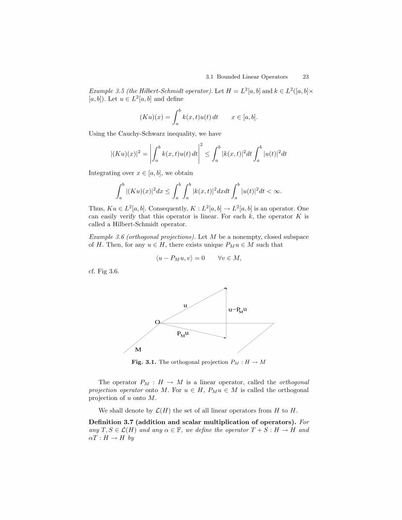
Example 3.6 (orthogonal projections). Let M be a nonempty, closed subspaceof H. Then, for any u ∈ H, there exists unique PMu ∈ M such that

〈u − PMu, v〉 = 0 ∀v ∈ M,

cf. Fig 3.6.

uu−P

M

PMu

O

uM

Fig. 3.1. The orthogonal projection PM : H → M

The operator PM : H → M is a linear operator, called the orthogonalprojection operator onto M . For u ∈ H, PMu ∈ M is called the orthogonalprojection of u onto M .

We shall denote by L(H) the set of all linear operators from H to H.

Definition 3.7 (addition and scalar multiplication of operators). Forany T, S ∈ L(H) and any α ∈ F, we define the operator T + S : H → H andαT : H → H by


(T + S)u = Tu + Su ∀u ∈ H,

(αT )u = αTu ∀α ∈ F, ∀u ∈ H.

The proof of the following proposition is left as an exercise problem, cf.Problem 3.1.

Proposition 3.8. With respect to the operations defined in Definition 3.7,the set L(H) is a vector space over F.

Definition 3.9 (continuity and boundedness of operators). Let T ∈L(H).

(1) The operator T is continuous, if

limk→∞

Tuk = Tu in H, whenever limk→∞

uk = u in H.

(2) The operator T is bounded, if there exists a constant M > 0 such that

‖Tu‖ ≤ M‖u‖ ∀u ∈ H. (3.6)

Proposition 3.10. Let T ∈ L(H). Then, the following are equivalent:

(1) The operator T : H → H is continuous;(2) The operator T : H → H is continuous at o, i.e.,

limk→∞

Tuk = o in H, whenever limk→∞

uk = o in H;

(3) The operator T : H → H is bounded;(4) For any bounded set E ⊆ H, the image T (E) = {Tu : u ∈ E} is bounded

in H.

Proof. (1) =⇒ (2). This follows from setting u = o in Part (1) of Definition 3.9.(2) =⇒ (1). Suppose uk → u in H. Then, uk − u → o in H. By Proposi-

tion 3.2 and (2),

T (uk − u) = Tuk − Tu → o. in H.

Hence,Tuk → Tu in H.

This proves (1).(3) =⇒ (2). If uk → o, then by (3)

‖Tuk‖ ≤ M‖uk‖ → 0 as k → ∞,

implying (2).(2) =⇒ (3). Assume (2) is true. If (3) were not true, then, for any k ∈ N

there exists uk ∈ H such that


‖Tuk‖ > M‖uk‖ k = 1, · · · . (3.7)

Clearly, by this and Part (1) of Proposition 3.2, each uk (k ≥ 1) is nonzero.Moreover, setting

vk =1

k‖uk‖uk, k = 1, · · · ,

we have

‖vk‖ =1

k→ 0 as k → ∞.

But, by (3.7),‖Tuk‖ > 1, k = 1, · · · ,

contradicting (2). Therefore, (3) is true.(3) =⇒ (4). If E ⊆ H is a bounded set, then there exists C > 0 such that

‖u | ≤ C ∀u ∈ E.

Thus,‖Tu‖ ≤ ‖T‖ ‖u‖ ≤ C‖T‖ ∀u ∈ E.

Hence, T (E) is bounded.(4) =⇒ (3). Setting

E = {u ∈ H : ‖u‖ = 1},

we haveM := sup

u∈H,‖u‖=1

‖Tu‖ < ∞.

Since (1/‖u‖)u ∈ E for any u ∈ H with u 6= o,

1

‖u‖‖Tu‖ =

∥

∥

∥

∥

T

(

1

‖u‖u

)∥

∥

∥

∥

≤ M ∀u ∈ H, u 6= o.

This implies (3.6). Hence, T is bounded. ⊓⊔

We shall denote by B(H) the set of all the bounded linear operators in H.

Definition 3.11. For any T ∈ B(H), we define

‖T‖ = supu∈H,u6=o

‖Tu‖

‖u‖. (3.8)

By Definition 3.9, ‖T‖ is finite for any T ∈ B(H).

Proposition 3.12. Let T ∈ B(H). Then,

‖T‖ = supu∈H,‖u‖≤1

‖Tu‖ = supu∈H,‖u‖=1

‖Tu‖, (3.9)

‖Tu‖ ≤ ‖T‖‖u‖ ∀u ∈ H. (3.10)


Proof. By (3.8),

supu∈H,‖u‖=1

‖Tu‖ ≤ supu∈H,‖u‖≤1

‖Tu‖ ≤ ‖T‖. (3.11)

If u ∈ H and u 6= o, then v = (1/‖u‖)u is a unit vector. Thus,

‖Tu‖

‖u‖= ‖Tv‖ ≤ sup

u∈H,‖u‖=1

‖Tu‖.

Hence, by (3.8),‖T‖ ≤ sup

u∈H,‖u‖=1

‖Tu‖.

This and (3.11) imply (3.9).The inequality (3.10) follows from the definition (3.8). ⊓⊔

Theorem 3.13. The set B(H) is a Banach space with respect to the opera-tions in L(H) and ‖ · ‖ : B(H) → R.

Proof. Step 1. The set B(H) is a vector subspace of the vector subspace L(H).Obviously, the zero operator O ∈ B(H). So, B(H) 6= ∅. Let T, S ∈ B(H).

Then,

‖(T + S)u‖ = ‖Tu + Su‖ ≤ ‖Tu‖ + ‖Su‖

≤ ‖T‖‖u‖ + ‖S‖‖u‖ = (‖T‖ + ‖S‖)‖u‖ ∀u ∈ H. (3.12)

Hence, T + S ∈ B(H). Let T ∈ B(H) and α ∈ F. Then,

‖(αT )u‖ = ‖α(Tu)‖ = |α|‖Tu‖ ≤ |α|‖T‖‖u‖ ∀u ∈ H.

Hence, αT ∈ B(H). Therefore, by ?, B(H) is a vector subspace of L(H).Step 2. The vector space B(H) is a normed vector space with respect to

‖ · ‖ : B(H) → R defined in (3.8).(1) Clearly,

‖T‖ ≥ 0 ∀T ∈ B(H).

By (3.8) and (3.1), for T ∈ B(H),

‖T‖ = 0 if and only if T = o.

(2) Let T ∈ B(H) and α ∈ F. By (3.8),

‖αT‖ = supu∈H,u6=o

‖(αT )u‖ = supu∈H,u6=o

‖α(Tu)‖

= supu∈H,u6=o

|α|‖Tu‖ = |α| supu∈H,u6=o

‖(αT )u‖ = |α|‖T‖.

(3) Let T, S ∈ B(H). It follows from (3.12) and (3.8) that


‖T + S‖ ≤ ‖T‖ + ‖S‖.

It follows from (1)–(3) that B(H) is a normed vector space.Step 3. The normed vector space B(H) is a Banach space.Let {Tn}

∞n=1 be a Cauchy sequence in B(H). Then, for any u ∈ H,

{Tnu}∞n=1 is a Cauchy sequence in H, since

‖Tmu − Tnu‖ ≤ ‖Tm − Tn‖‖u‖ → 0 as m,n → ∞.

Since H is a Hilbert space, {Tnu}∞n=1 converges in H. We define

Tu = limn→∞

Tnu in H. (3.14)

Clearly, T : H → H is linear, since

T (u + v) = limn→∞

Tn(u + v) = limn→∞

(Tnu + Tnv)

= limn→∞

Tnu + limn→∞

Tnv = Tu + Tv ∀u, v ∈ H,

T (αu) = limn→∞

Tn(αu) = limn→∞

α(Tnu)

= α limn→∞

Tnu = αTu ∀u, v ∈ H.

By (3.14), we have

‖Tu‖ = limn→∞

‖Tnu‖ ≤

(

supn≥1

‖Tn‖

)

‖u‖ = M‖u‖ ∀u ∈ H,

whereM = sup

n≥1‖Tn‖ < ∞,

since {Tn}∞n=1 is a Cauchy sequence and hence a bounded sequence in B(H).

Therefore, T ∈ B(H).Finally, let ε > 0. Since {Tn}

∞n=1 is a Cauchy sequence in B(H), there

exists N ∈ N such that

‖Tm − Tn‖ < ε ∀m,n ≥ N.

Let u ∈ H with ‖u‖ = 1. We thus have

‖Tmu − Tnu‖ ≤ ‖Tm − Tn‖ · ‖u‖ < ε ∀m,n ≥ N.

Sending n → ∞, we obtain

‖Tmu − Tu‖ ≤ ε ∀m ≥ N.

This, together with (3.9), leads to

‖Tm − T‖ ≤ ε ∀m ≥ N,

i.e.,lim

m→∞Tm = T in B(H).

Consequently, B(H) is a Banach space. ⊓⊔.


Example 3.14. Let H = Fn. Then, B(H) = L(H).

Definition 3.15 (multiplication of operators). Let T, S ∈ B(H). We de-fine TS : H → H by

(TS)u = T (Su) ∀u ∈ H.

We also define

T 0 = I and T k = T k−1T, k = 1, · · · .

Proposition 3.16. If T, S ∈ B(H), then TS ∈ B(H). Moreover,

‖TS‖ ≤ ‖T‖ ‖S‖. (3.15)

In particular,∥

∥T k∥

∥ ≤ ‖T‖k k = 0, 1, · · · . (3.16)

Proof. We have for any u, v ∈ H and any α ∈ F that

(TS)(u + v) = T (S(u + v)) = T (Su + Sv)

= T (Su) + T (Sv) = (TS)u + (TS)v,

(TS)(αu) = T (S(αu)) = T (αSu) = αT (Su) = α(TS)u.

Thus, TS : H → H is linear.The boundedness of TS and (3.15) follow from the following:

‖(TS)u‖ = ‖T (Su)‖ ≤ ‖T‖ ‖Su‖ ≤ ‖T‖ ‖S‖ ‖u‖ ∀u ∈ H. ⊓⊔.

The following result is straightforward, and its proof is omitted.

Proposition 3.17. Let R,S, T ∈ B(H) and α ∈ F. Then,

(RS)T = R(ST ), (3.17)

R(S + T ) = RS + RT, (3.18)

(R + S)T = RS + ST, (3.19)

(αS)T = α(ST ) = S(αT ). (3.20)

A Banach algebra over F is a normed vector space over F on which amultiplication is defined so that (3.17)–(3.20) and (3.15) hold true for allR,S, T in the space and all α ∈ F. By Proposition 3.16 and Proposition 3.17,we have the following corollary.

Corollary 3.18. For any Hilbert space H over F, the set B(H) of all boundedlinear operators on H is a Banach algebra over F.

Proposition 3.19. (1) If Tn → T in B(H), then

Tnu → Tu ∀u ∈ H.


(2) If Tn → T and Sn → S in B(H), then

TnSn → TS.

Proof. (1) For any u ∈ H, we have by (3.10),

‖Tnu − Tu‖ ≤ ‖Tn − T‖ ‖u‖ → 0 as n → ∞.

(2) Since {Tn}∞n=1 converges in B(H), it is bounded. Thus, by the triangle

inequality and (3.15), we have

‖TnSn − TS‖ = ‖(Tn − T )Sn + T (Sn − S)‖

≤ ‖(Tn − T )Sn‖ + ‖T (Sn − S)‖

≤ ‖Tn − T‖ ‖Sn‖ + ‖T‖ ‖Sn − S‖

→ 0 as n → ∞.

completing the proof. ⊓⊔

Example 3.20. Let H be a Hilbert space over F with a countable orthonormalbasis {en}

∞n=1. Each u ∈ H then has a unique Fourier expansion (cf. ?)

u =

∞∑

k=1

〈u, ek〉ek.

Define Tn : H → H for each n ∈ N by

Tnu =

n∑

k=1

〈u, ek〉ek.

Clearly, Tn is the projection onto

Mn := span {e1, · · · , en}.

Hence, Tn ∈ B(H). Moreover,

‖Tn‖ = 1 ∀n ∈ N.

In particular, {Tn}∞n=1 does not converge to the zero operator O : H → H in

B(H).However, for any u ∈ H,

‖Tnu‖2 =n

∑

k=1

|〈u, ek〉|2 → 0 as n → ∞.

Hence, the converse of Part (1) in Proposition 3.19 is in general not true.


Definition 3.21 (invertible operators). Let S, T ∈ B(H). If

ST = TS = I, (3.21)

then T is invertible, and S is an inverse of T .

Proposition 3.22. If T ∈ B(H) is invertible, then its inverse is unique.

Proof. Let R,S ∈ B(H) be inverses of T . Then,

R = RI = R(TS) = (RT )S = IS = S. ⊓⊔

If T ∈ B(H) is invertible, we shall denote by T−1 its unique inverse.

Theorem 3.23 (The von Neumann series). Let T ∈ B(H). Suppose‖T‖ < 1. Then, I − T ∈ B(H) is invertible. Moreover,

(I − T )−1 =∞∑

k=0

T k.

Proof. For each n ∈ N, set Let

Sn =n

∑

k=0

T k n = 1, · · · .

Since ‖T‖ < 1, the series∑∞

k=0 ‖T‖k converges. Thus, for any p ∈ N, we haveby (3.16) that

‖Sn+p − Sn‖ =

∥

∥

∥

∥

∥

n+p∑

k=n+1

T k

∥

∥

∥

∥

∥

≤

n+p∑

k=n+1

∥

∥T k∥

∥ ≤∞∑

k=n+1

‖T‖k → 0 as n → ∞.

Hence, {Sn}∞n=1 is a Cauchy sequence in H, and therefore it converges in H.

This shows that the series∑∞

k=10 T k converges in H, and

Sn →∞∑

k=10

T k in H. (3.22)

One can easily verify that

(I − T )Sn = Sn(I − T ) = I − Tn+1.

Sending n → ∞, we obtain then by (3.22) and Part (2) of Proposition 3.19that

(I − T )

∞∑

k=10

T k =

(

∞∑

k=10

T k

)

(I − T ) = I,

completing the proof. ⊓⊔

3.3 Compact Operators 31

3.2 Self-Adjoint Operators

3.3 Compact Operators

Definition 3.24 (compact operators). An operator T ∈ B(H) is a com-pact operator, if for any bounded squence {un}

∞n=1 in H, there exists a sub-

sequence {unk}∞k=1 such that {Tunk

}∞k=1 converges in H.

Proposition 3.25. (1) If T, S ∈ B(H) are two compact operators and α ∈ F,then T + S and αT are also compact operators on H.

(2) If T ∈ B(H) is a compact operator and S ∈ B(H), then TS and ST arealso compact operators.

(3) If {Tn}∞n=1 is a sequence of compact operators on H and

Tn → T in B(H)

for some T ∈ B(H), then T is also a compact operator.

Proof. (1) Let {un}∞n=1 be a bounded sequence in H. Since T ∈ B(H) is com-

pact, there exists a subsequence {unk}∞k=1, of {un}

∞n=1 such that {Tunk

}∞k=1

converges in H. Clearly, {(αT )unk}∞k=1 also converges. Hence, αT ∈ B(H) is

compact. Moreover, there exists a further subsequence, {unkj}∞j=1, of {unk

}∞=1

such that {Sunkj}∞j=1 converges in H, since S ∈ B(H) is compact. Thus,

{(T + S)unkj}∞j=1 converges in H. This implies that T + S ∈ B(H) is com-

pact.(2) Let {un}

∞n=1 be a bounded sequence in H. Since S ∈ B(H), {Sun}

∞n=1

is also bounded in H. Thus, since T ∈ B(H) is compact and

(TS)un = T (Sun), n = 1, · · · ,

there exists a subsequence, {unk}∞k=1, of {un}

∞n=1 such that {(TS)unk

}∞k=1

converges. Hence, TS ∈ B(H) is compact.Since T is compact, there exists a subsequence {unk

}∞k=1, of {un}∞n=1 such

that {Tunk}∞k=1 converges. Since S ∈ B(H), {(ST )unk

}∞k=1 also converges.Hence, ST is also compact.

(3) Let again {un}∞n=1 be a bounded sequence in H. There exists A > 0

such that‖un‖ ≤ A, n = 1, · · · . (3.23)

Since T1 is compact, there exists a subsequence, {u(1)n }∞n=1, of {un}

∞n=1

such that {T1u(1)n }∞n=1 converges in H. Suppose {u

(k)n }∞n=1 is a subsequence

of {un}∞n=1 such that {Tku

(k)n }∞n=1 converges in H. Then, since Tk+1 is

compact, there exists a subsequence, {u(k+1)n }∞n=1, of {u

(k)n }∞n=1 such that

{Tk+1u(k+1)n }∞n=1 converges in H. Thus, by induction, for each k ∈ F, there

exists a subsequence {u(k)n }∞n=1 of {u

(k−1)n }∞n=1, with {u

(0)n }∞n=1 being {un}

∞n=1,

such that {Tku(k)n }∞n=1 converges. Let


vn = u(n)n , n = 1, · · · .

Then, {vn}∞n=1 is a subsequence of {un}

∞n=1, and for each k ∈ N, {Tkun}

∞n=1

converges in H.We need now only to show that the sequence {Tvn}

∞n=1 converges in H.

Let ε > 0. Since Tn → T in B(H), there exists N ∈ N such that

‖Tk − T‖ ≤ ε∀k ≥ N. (3.24)

Since {TNvn}∞n=1 converges, it is a Cauchy sequence. Thus, there exists L ∈ N

such that‖TNvp − TNvq‖ ≤ ε ∀p, q ∈ N with p, q ≥ L. (3.25)

Consequently, by (3.10), (3.23), (3.24), and (3.25),

‖Tvp − Tvq‖ ≤ ‖Tvp − TNvp‖ + ‖TNvp − TNvq‖ + ‖TNvq − Tvq‖

≤ ‖T − TN‖ ‖vp‖ + ‖TNvp − TNvq‖ + ‖TN − T‖ ‖vq‖

≤ 2Aε + ε ∀p, q ∈ N with p, q ≥ L.

Hence, {Tvn}∞n=1 is a Cauchy sequence, and it thus converges in H. ⊓⊔

We shall denote by C(H) the set of all compact operators on H.

Proposition 3.26. The set C(H) is a Banach algebra.

Proof. Note that the zero operator O : H → H is a compact operator. Thus,C(H) is nonempty. Note also that C(H) ⊆ B(H). By Proposition 3.25, C(H)is closed under addition, scalar multiplication, and multiplication. It is alsoclosed with respect to the norm of B(H). Therefore, C(H) is a sub-Banachalgebra of B(H). Hence, it is itself a Banach algebra. ⊓⊔

If T ∈ L(H), then the image of T : H → H,

T (H) = {Tu : u ∈ H},

is a subspace of H. We call the dimension of T (H) the rank of T .

Proposition 3.27. If T ∈ B(H) has a finite rank, then T is compact.

Proof. ⊓⊔

Exercises


References

4

Integral Equations

4.1 Examples and Classification of Integral Equatons

4.2 Integral Equations of the Second Kind: Successive

Iterations

4.3 Fredholm Theory of Integral Equations of the

Second Kind

4.4 Singular Integral Equations

Exercises

References

A

Appendix

A.1 Zorn’s Lemma

Given a set S. Let ≤ be a relation of S, i.e., for some x, y ∈ S, either x ≤ yor y ≤ x.

Definition A.1. A relation ≤ of a set S is a partial order, if the followingare satisfied:

(1) For any x ∈ S, x ≤ x;(2) For any x, y ∈ S, x ≤ y and y ≤ x imply x = y;(3) For any x, y, z ∈ S, x ≤ y and y ≤ z imply x ≤ z.

Definition A.2. Let S be a partially ordered set with the partial order ≤.

(1) A subset C ⊆ S is a chain, if either x ≤ y or y ≤ x for any x, y ∈ C.(2) An element m ∈ S is a maximal element of S, if x ∈ S and m ≤ x imply

that x = m.

We hypothesize the following

Zorn’s Lemma. A partially ordered set in wich any chain has an upper boundcontains a maximal element.

A.2 Cardinality

Definition A.3. Let S and T be two sets. A mapping ϕ : S → T is:

(1) injective, if ϕ(s1) 6= ϕ(s2) for any s1, s2 ∈ S with s1 6= s2;(2) surjective, if for any t ∈ T , there exists s ∈ S such that t = ϕ(s);(3) bijective, if it is both injective and surjective.

36 A Appendix

Two sets S and T are said to be equipllent, denoted by S ∼ B, if thereexists a bijective mapping from S to T . Clearly, equipllence is an equivalencerelation on the class of all sets, i.e., for any sets R,S, T : S ∼ S; S ∼ T impliesT ∼ S; and R ∼ S and S ∼ T imply R ∼ T .

Any set S is therefore associated with a unique cardinal nubmer, or cardi-nality, denoted by cardS, that is characterized by

card S = card T if and only if S ∼ T.

For two sets S and T , we say card S < cardT , if cardS 6= card T and thereexists T0 ( T such that cardS = cardT0.

If S is a finite set, then cardS is the number of elements in S. If S is infiniteand cardS = card N, then S is said to be countably infinite or countable. Thecardinal number of a countably infinite set is denoted by ℵ0 (ℵ is pronouncedaleph). If S is infinite but cardS 6= card N, then S is said to be uncountablyinfinite or uncountable.

For example, the set of positive integers N, the set of all integers Z, and theset of all rational numbers Q are all countable. The set {x ∈ R : 0 < x < 1},the set of real numbers R, the set of all complex numbers C, the set Cn forany integer n ∈ N are all uncountable. They have the same cardinal number,denoted by ℵ. One can verify that ℵ0 < ℵ.

elements of hilbert space and operator theory · chapter 1 reviews vector spaces: bases, subspaces,...

Documents