elementary data structures stacks, queues, lists, vectors, sequences, trees, priority queues, heaps,...
TRANSCRIPT
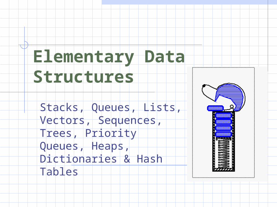
Elementary Data Structures
Stacks, Queues, Lists, Vectors, Sequences, Trees, Priority Queues, Heaps, Dictionaries & Hash Tables

Elementary Data Structures 2
The Stack ADT (§2.1.1)The Stack ADT stores arbitrary objectsInsertions and deletions follow the last-in first-out schemeThink of a spring-loaded plate dispenserMain stack operations:
push(object): inserts an element
object pop(): removes and returns the last inserted element
Auxiliary stack operations:
object top(): returns the last inserted element without removing it
integer size(): returns the number of elements stored
boolean isEmpty(): indicates whether no elements are stored

Elementary Data Structures 3
Applications of Stacks
Direct applications Page-visited history in a Web browser Undo sequence in a text editor Chain of method calls in the Java
Virtual Machine or C++ runtime environment
Indirect applications Auxiliary data structure for algorithms Component of other data structures

Elementary Data Structures 4
The Queue ADT (§2.1.2)The Queue ADT stores arbitrary objectsInsertions and deletions follow the first-in first-out schemeInsertions are at the rear of the queue and removals are at the front of the queueMain queue operations:
enqueue(object): inserts an element at the end of the queue
object dequeue(): removes and returns the element at the front of the queue
Auxiliary queue operations:
object front(): returns the element at the front without removing it
integer size(): returns the number of elements stored
boolean isEmpty(): indicates whether no elements are stored
Exceptions Attempting the execution
of dequeue or front on an empty queue throws an EmptyQueueException
Elementary Data Structures 5
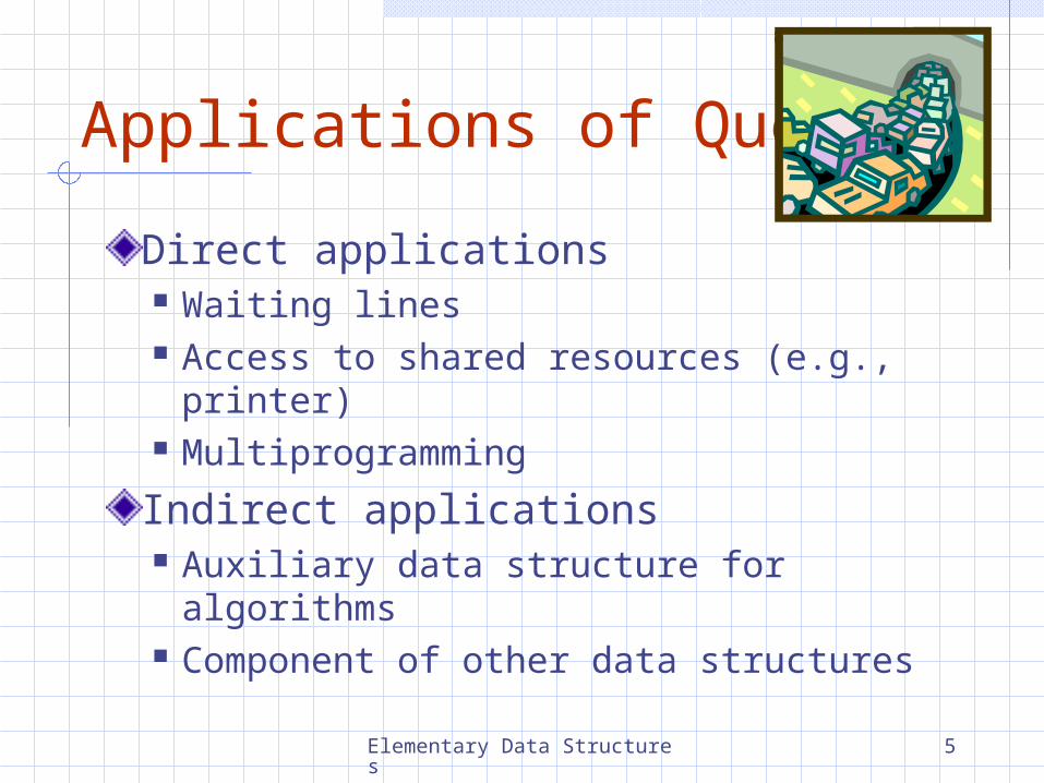
Applications of Queues
Direct applications Waiting lines Access to shared resources (e.g.,
printer) Multiprogramming
Indirect applications Auxiliary data structure for algorithms Component of other data structures

Elementary Data Structures 6
Position ADTThe Position ADT models the notion of place within a data structure where a single object is storedIt gives a unified view of diverse ways of storing data, such as a cell of an array a node of a linked list
Just one method: object element(): returns the element
stored at the position

Elementary Data Structures 7
List ADT (§2.2.2)
The List ADT models a sequence of positions storing arbitrary objectsIt allows for insertion and removal in the “middle” Query methods:
isFirst(p), isLast(p)
Accessor methods: first(), last() before(p), after(p)
Update methods: replaceElement(p,
o), swapElements(p, q)
insertBefore(p, o), insertAfter(p, o),
insertFirst(o), insertLast(o)
remove(p)
Elementary Data Structures 8
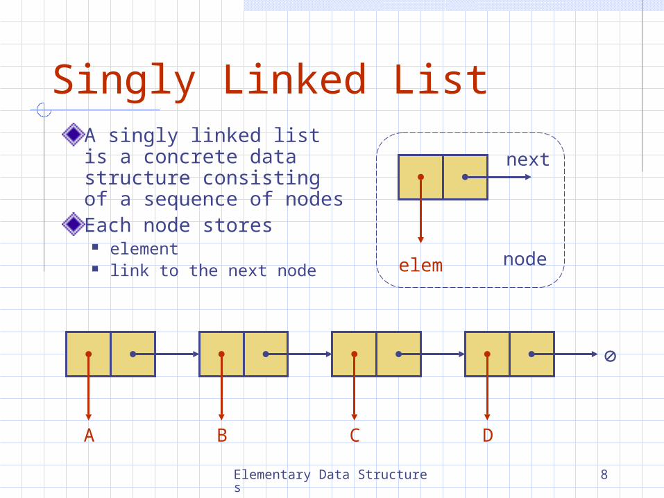
Singly Linked ListA singly linked list is a concrete data structure consisting of a sequence of nodesEach node stores
element link to the next node
next
elem node
A B C D
Elementary Data Structures 9
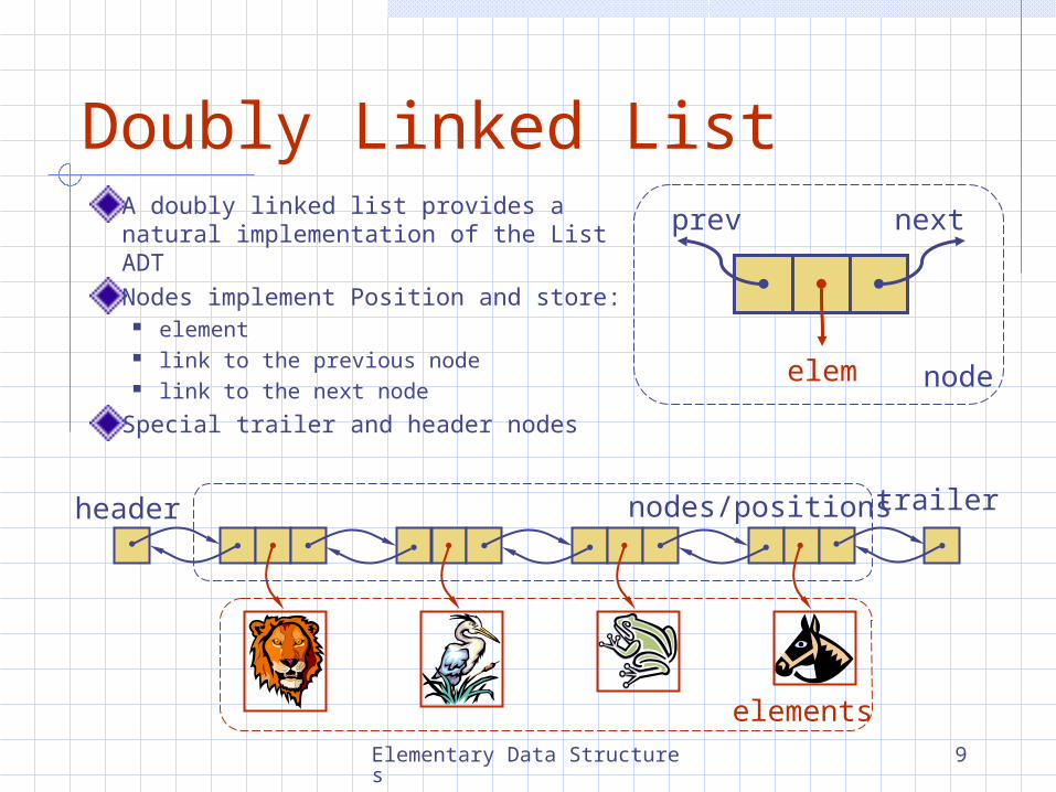
Doubly Linked ListA doubly linked list provides a natural implementation of the List ADTNodes implement Position and store:
element link to the previous node link to the next node
Special trailer and header nodes
prev next
elem
trailerheader nodes/positions
elements
node

Elementary Data Structures 10
The Vector ADTThe Vector ADT extends the notion of array by storing a sequence of arbitrary objectsAn element can be accessed, inserted or removed by specifying its rank (number of elements preceding it)An exception is thrown if an incorrect rank is specified (e.g., a negative rank)
Main vector operations: object elemAtRank(integer r):
returns the element at rank r without removing it
object replaceAtRank(integer r, object o): replace the element at rank with o and return the old element
insertAtRank(integer r, object o): insert a new element o to have rank r
object removeAtRank(integer r): removes and returns the element at rank r
Additional operations size() and isEmpty()

Elementary Data Structures 11
Applications of Vectors
Direct applications Sorted collection of objects
(elementary database)
Indirect applications Auxiliary data structure for algorithms Component of other data structures
Elementary Data Structures 12
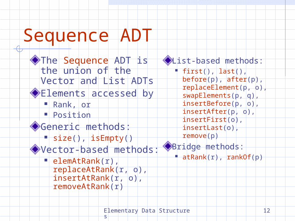
Sequence ADTThe Sequence ADT is the union of the Vector and List ADTsElements accessed by
Rank, or Position
Generic methods: size(), isEmpty()
Vector-based methods: elemAtRank(r),
replaceAtRank(r, o), insertAtRank(r, o), removeAtRank(r)
List-based methods: first(), last(),
before(p), after(p), replaceElement(p, o), swapElements(p, q), insertBefore(p, o), insertAfter(p, o), insertFirst(o), insertLast(o), remove(p)
Bridge methods: atRank(r), rankOf(p)
Elementary Data Structures 13
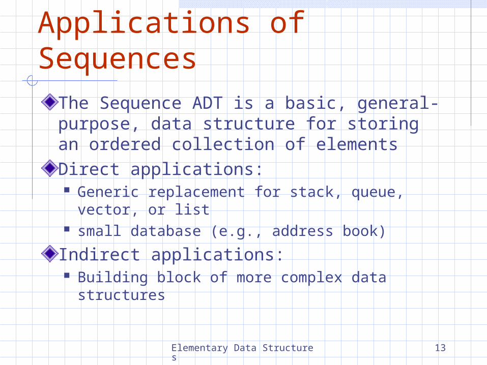
Applications of SequencesThe Sequence ADT is a basic, general-purpose, data structure for storing an ordered collection of elementsDirect applications: Generic replacement for stack, queue, vector,
or list small database (e.g., address book)
Indirect applications: Building block of more complex data structures

Elementary Data Structures 14
Trees (§2.3)In computer science, a tree is an abstract model of a hierarchical structureA tree consists of nodes with a parent-child relationApplications:
Organization charts File systems Programming
environments
Computers”R”Us
Sales R&DManufacturing
Laptops DesktopsUS International
Europe Asia Canada

Elementary Data Structures 15subtree
Tree TerminologyRoot: node without parent (A)Internal node: node with at least one child (A, B, C, F)External node (a.k.a. leaf ): node without children (E, I, J, K, G, H, D)Ancestors of a node: parent, grandparent, grand-grandparent, etc.Depth of a node: number of ancestorsHeight of a tree: maximum depth of any node (3)Descendant of a node: child, grandchild, grand-grandchild, etc.
A
B DC
G HE F
I J K
Subtree: tree consisting of a node and its descendants

Elementary Data Structures 16
Tree ADT (§2.3.1)We use positions to abstract nodesGeneric methods:
integer size() boolean isEmpty() objectIterator elements() positionIterator
positions()
Accessor methods: position root() position parent(p) positionIterator
children(p)
Query methods: boolean isInternal(p) boolean isExternal(p) boolean isRoot(p)
Update methods: swapElements(p, q) object replaceElement(p,
o)
Additional update methods may be defined by data structures implementing the Tree ADT
Elementary Data Structures 17
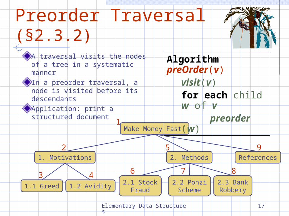
Preorder Traversal (§2.3.2)A traversal visits the nodes of a tree in a systematic mannerIn a preorder traversal, a node is visited before its descendants Application: print a structured document
Make Money Fast!
1. Motivations References2. Methods
2.1 StockFraud
2.2 PonziScheme
1.1 Greed 1.2 Avidity2.3 BankRobbery
1
2
3
5
4 6 7 8
9
Algorithm preOrder(v)visit(v)for each child w of v
preorder (w)
Elementary Data Structures 18
Postorder Traversal (§2.3.2)
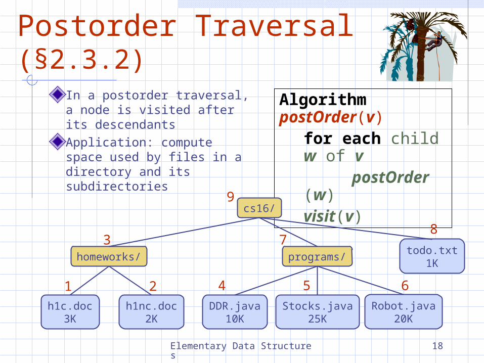
In a postorder traversal, a node is visited after its descendantsApplication: compute space used by files in a directory and its subdirectories
Algorithm postOrder(v)for each child w of v
postOrder (w)visit(v)
cs16/
homeworks/todo.txt
1Kprograms/
DDR.java10K
Stocks.java25K
h1c.doc3K
h1nc.doc2K
Robot.java20K
9
3
1
7
2 4 5 6
8
Elementary Data Structures 19
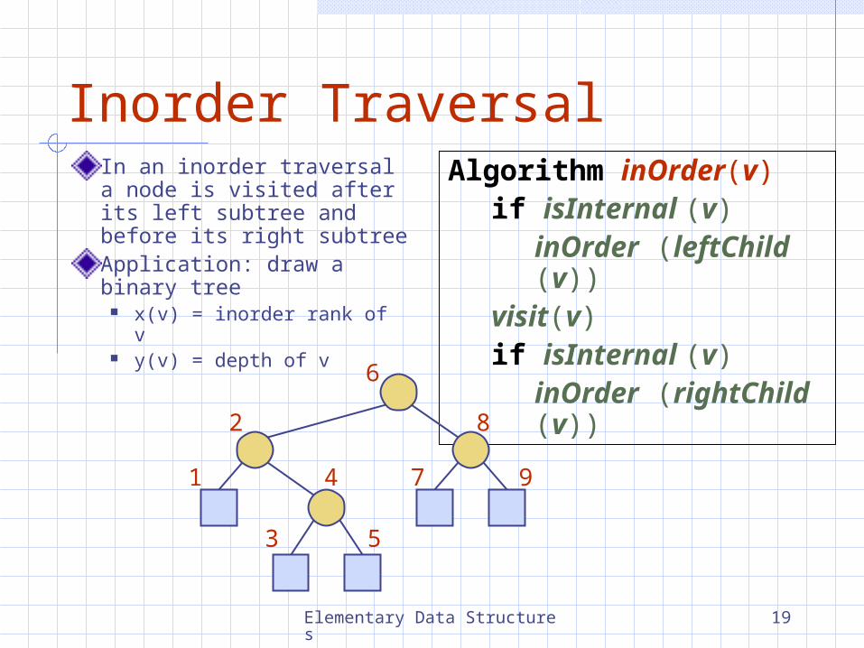
Inorder TraversalIn an inorder traversal a node is visited after its left subtree and before its right subtreeApplication: draw a binary tree
x(v) = inorder rank of v y(v) = depth of v
Algorithm inOrder(v)if isInternal (v)
inOrder (leftChild (v))visit(v)if isInternal (v)
inOrder (rightChild (v))
3
1
2
5
6
7 9
8
4
Elementary Data Structures 20
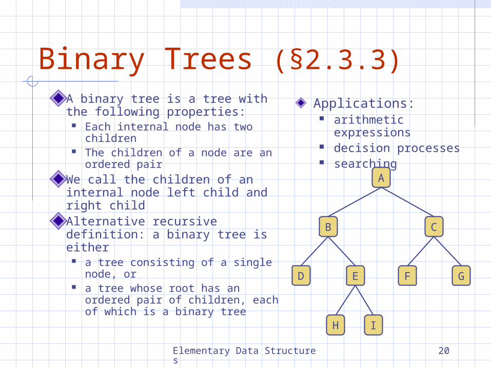
Binary Trees (§2.3.3)A binary tree is a tree with the following properties:
Each internal node has two children
The children of a node are an ordered pair
We call the children of an internal node left child and right childAlternative recursive definition: a binary tree is either
a tree consisting of a single node, or
a tree whose root has an ordered pair of children, each of which is a binary tree
Applications: arithmetic
expressions decision processes searching
A
B C
F GD E
H I
Elementary Data Structures 21
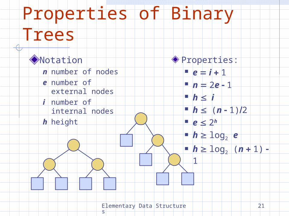
Properties of Binary TreesNotationn number of nodese number of
external nodesi number of
internal nodesh height
Properties: e i 1 n 2e 1 h i h (n 1)2 e 2h
h log2 e
h log2 (n 1) 1
Elementary Data Structures 22
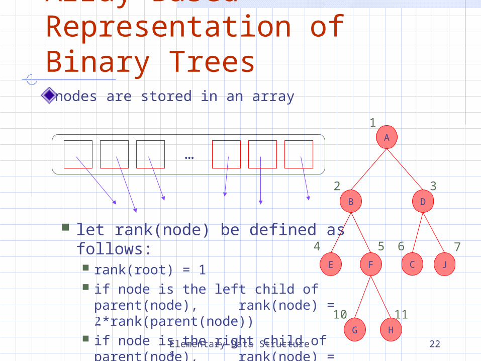
Array-Based Representation of Binary Trees
nodes are stored in an array
…
let rank(node) be defined as follows: rank(root) = 1 if node is the left child of parent(node),
rank(node) = 2*rank(parent(node)) if node is the right child of parent(node),
rank(node) = 2*rank(parent(node))+1
1
2 3
6 74 5
10 11
A
HG
FE
D
C
B
J

Elementary Data Structures 23
Priority Queue ADT
A priority queue stores a collection of itemsAn item is a pair(key, element)Main methods of the Priority Queue ADT
insertItem(k, o)inserts an item with key k and element o
removeMin()removes the item with smallest key and returns its element
Additional methods minKey(k, o)
returns, but does not remove, the smallest key of an item
minElement()returns, but does not remove, the element of an item with smallest key
size(), isEmpty()Applications:
Standby flyers Auctions Stock market
Elementary Data Structures 24
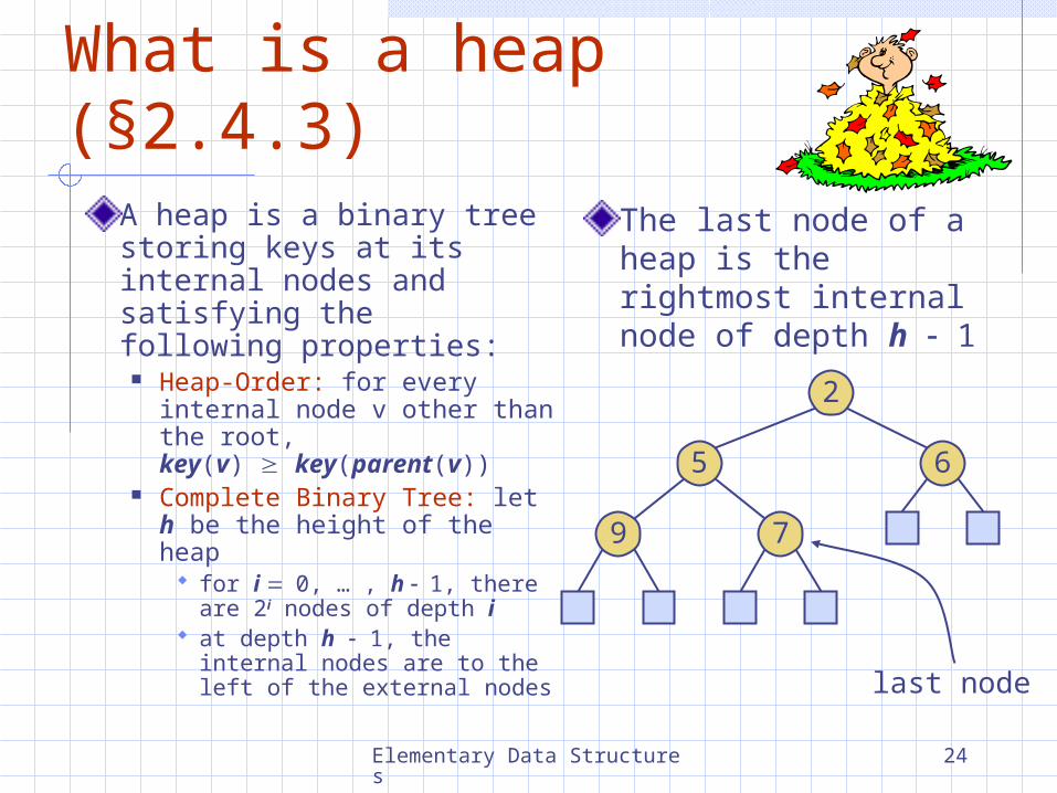
What is a heap (§2.4.3)A heap is a binary tree storing keys at its internal nodes and satisfying the following properties:
Heap-Order: for every internal node v other than the root,key(v) key(parent(v))
Complete Binary Tree: let h be the height of the heap
for i 0, … , h 1, there are 2i nodes of depth i
at depth h 1, the internal nodes are to the left of the external nodes
2
65
79
The last node of a heap is the rightmost internal node of depth h 1
last node
Elementary Data Structures 25
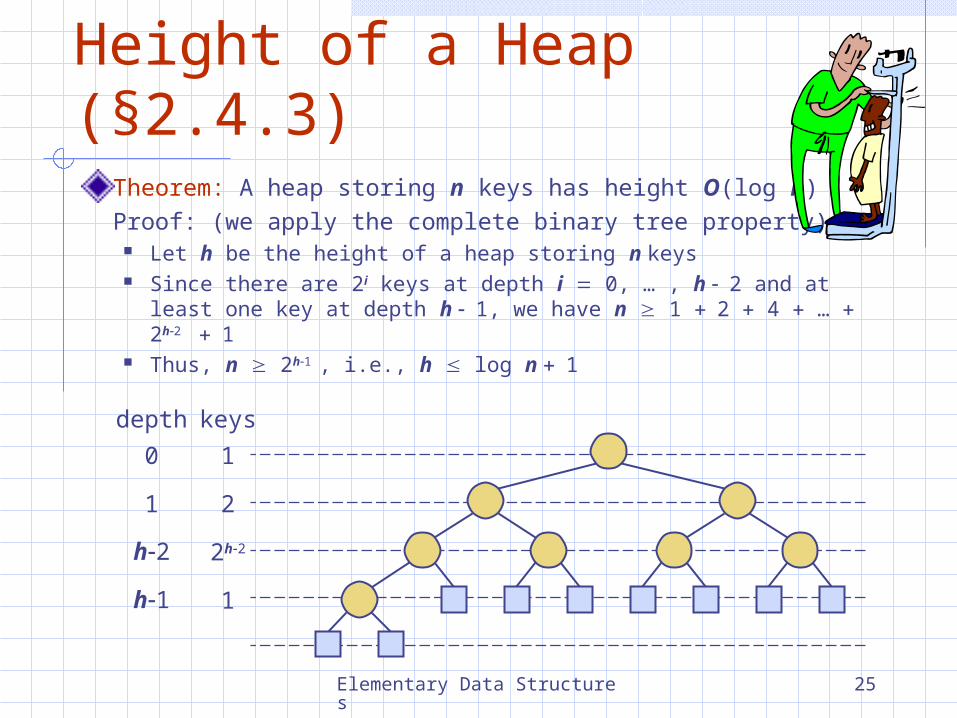
Height of a Heap (§2.4.3)Theorem: A heap storing n keys has height O(log n)
Proof: (we apply the complete binary tree property) Let h be the height of a heap storing n keys Since there are 2i keys at depth i 0, … , h 2 and at least
one key at depth h 1, we have n 1 2 4 … 2h2 1
Thus, n 2h1 , i.e., h log n 1
1
2
2h2
1
keys
0
1
h2
h1
depth
Elementary Data Structures 26
Dictionary ADTThe dictionary ADT models a searchable collection of key-element itemsThe main operations of a dictionary are searching, inserting, and deleting itemsMultiple items with the same key are allowedApplications:
address book credit card authorization mapping host names (e.g.,
cs16.net) to internet addresses (e.g., 128.148.34.101)
Dictionary ADT methods: findElement(k): if the
dictionary has an item with key k, returns its element, else, returns the special element NO_SUCH_KEY
insertItem(k, o): inserts item (k, o) into the dictionary
removeElement(k): if the dictionary has an item with key k, removes it from the dictionary and returns its element, else returns the special element NO_SUCH_KEY
size(), isEmpty() keys(), Elements()

Elementary Data Structures 27
Binary SearchBinary search performs operation findElement(k) on a dictionary implemented by means of an array-based sequence, sorted by key
similar to the high-low game at each step, the number of candidate items is halved terminates after a logarithmic number of steps
Example: findElement(7)
1 3 4 5 7 8 9 11 14 16 18 19
1 3 4 5 7 8 9 11 14 16 18 19
1 3 4 5 7 8 9 11 14 16 18 19
1 3 4 5 7 8 9 11 14 16 18 19
0
0
0
0
ml h
ml h
ml h
lm h
Elementary Data Structures 28
Lookup TableA lookup table is a dictionary implemented by means of a sorted sequence
We store the items of the dictionary in an array-based sequence, sorted by key
We use an external comparator for the keys
Performance: findElement takes O(log n) time, using binary search insertItem takes O(n) time since in the worst case we have
to shift n2 items to make room for the new item removeElement take O(n) time since in the worst case we
have to shift n2 items to compact the items after the removal
The lookup table is effective only for dictionaries of small size or for dictionaries on which searches are the most common operations, while insertions and removals are rarely performed (e.g., credit card authorizations)

Elementary Data Structures 29
Binary Search TreeA binary search tree is a binary tree storing keys (or key-element pairs) at its internal nodes and satisfying the following property:
Let u, v, and w be three nodes such that u is in the left subtree of v and w is in the right subtree of v. We have key(u) key(v) key(w)
External nodes do not store items
An inorder traversal of a binary search trees visits the keys in increasing order
6
92
41 8
Elementary Data Structures 30
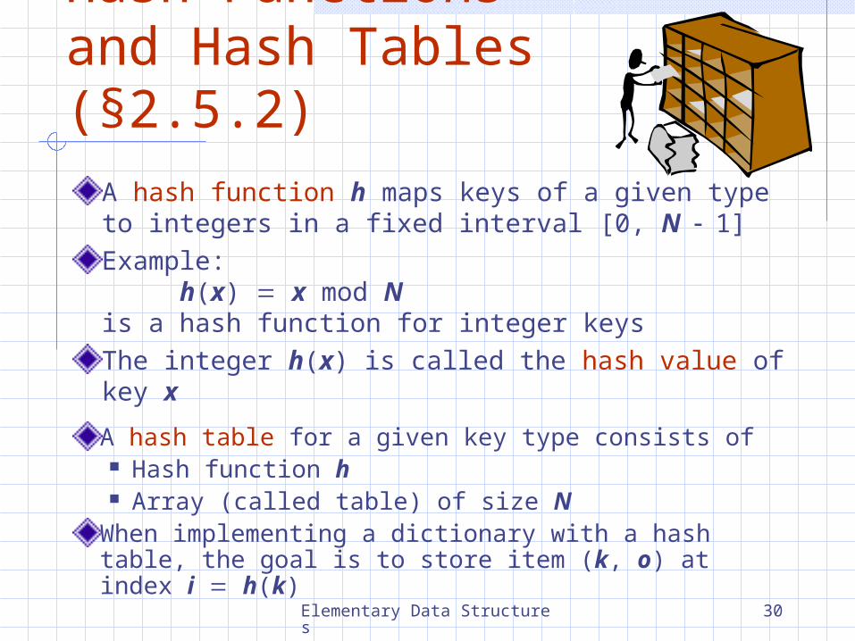
Hash Functions and Hash Tables (§2.5.2)
A hash function h maps keys of a given type to integers in a fixed interval [0, N1]
Example:h(x) x mod N
is a hash function for integer keysThe integer h(x) is called the hash value of key x
A hash table for a given key type consists of Hash function h Array (called table) of size N
When implementing a dictionary with a hash table, the goal is to store item (k, o) at index i h(k)
Elementary Data Structures 31
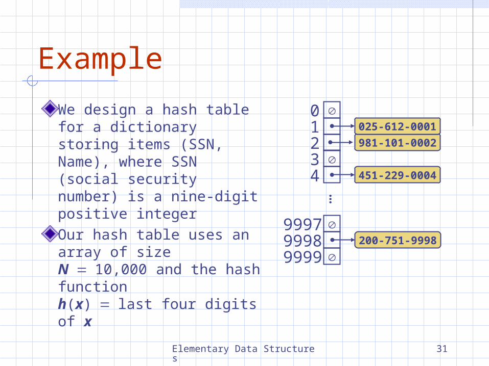
Example
We design a hash table for a dictionary storing items (SSN, Name), where SSN (social security number) is a nine-digit positive integerOur hash table uses an array of size N10,000 and the hash functionh(x)last four digits of x
01234
999799989999
…451-229-0004
981-101-0002
200-751-9998
025-612-0001

Elementary Data Structures 32
Hash Functions (§ 2.5.3)
A hash function is usually specified as the composition of two functions:Hash code map: h1: keys integers
Compression map: h2: integers [0, N1]
The hash code map is applied first, and the compression map is applied next on the result, i.e.,
h(x) = h2(h1(x))
The goal of the hash function is to “disperse” the keys in an apparently random way
Elementary Data Structures 33
Hash Code Maps (§2.5.3)
Memory address: We reinterpret the
memory address of the key object as an integer (default hash code of all Java objects)
Good in general, except for numeric and string keys
Integer cast: We reinterpret the bits of
the key as an integer Suitable for keys of length
less than or equal to the number of bits of the integer type (e.g., byte, short, int and float in Java)
Component sum: We partition the bits of
the key into components of fixed length (e.g., 16 or 32 bits) and we sum the components (ignoring overflows)
Suitable for numeric keys of fixed length greater than or equal to the number of bits of the integer type (e.g., long and double in Java)

Elementary Data Structures 34
Hash Code Maps (cont.)Polynomial accumulation:
We partition the bits of the key into a sequence of components of fixed length (e.g., 8, 16 or 32 bits) a0 a1 … an1
We evaluate the polynomialp(z) a0 a1 z a2 z2 …
… an1zn1
at a fixed value z, ignoring overflows
Especially suitable for strings (e.g., the choice z 33 gives at most 6 collisions on a set of 50,000 English words)
Polynomial p(z) can be evaluated in O(n) time using Horner’s rule:
The following polynomials are successively computed, each from the previous one in O(1) time
p0(z) an1
pi (z) ani1 zpi1(z) (i 1, 2, …, n 1)
We have p(z) pn1(z)
Elementary Data Structures 35
Compression Maps (§2.5.4)
Division: h2 (y) y mod N The size N of the
hash table is usually chosen to be a prime
The reason has to do with number theory and is beyond the scope of this course
Multiply, Add and Divide (MAD): h2 (y) (ay b) mod N a and b are
nonnegative integers such that
a mod N 0 Otherwise, every
integer would map to the same value b
Elementary Data Structures 36
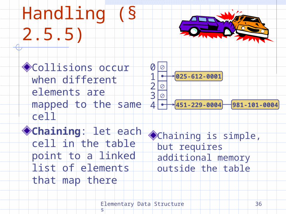
Collision Handling (§ 2.5.5)
Collisions occur when different elements are mapped to the same cellChaining: let each cell in the table point to a linked list of elements that map there
Chaining is simple, but requires additional memory outside the table
01234 451-229-0004 981-101-0004
025-612-0001
Elementary Data Structures 37
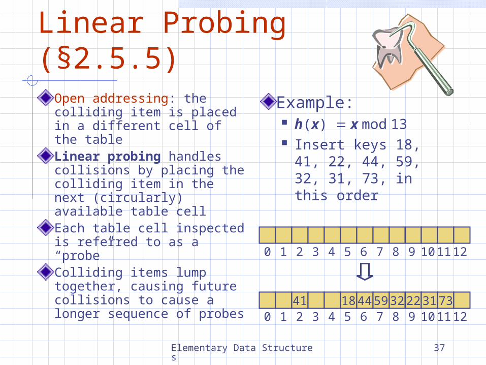
Linear Probing (§2.5.5)Open addressing: the colliding item is placed in a different cell of the tableLinear probing handles collisions by placing the colliding item in the next (circularly) available table cellEach table cell inspected is referred to as a “probe”Colliding items lump together, causing future collisions to cause a longer sequence of probes
Example: h(x) x mod 13 Insert keys 18, 41,
22, 44, 59, 32, 31, 73, in this order
0 1 2 3 4 5 6 7 8 9 10 11 12
41 18445932223173 0 1 2 3 4 5 6 7 8 9 10 11 12

Elementary Data Structures 38
Search with Linear ProbingConsider a hash table A that uses linear probingfindElement(k)
We start at cell h(k) We probe consecutive
locations until one of the following occurs
An item with key k is found, or
An empty cell is found, or
N cells have been unsuccessfully probed
Algorithm findElement(k)i h(k)p 0repeat
c A[i]if c
return NO_SUCH_KEY else if c.key () k
return c.element()else
i (i 1) mod Np p 1
until p Nreturn NO_SUCH_KEY

Elementary Data Structures 39
Updates with Linear Probing
To handle insertions and deletions, we introduce a special object, called AVAILABLE, which replaces deleted elementsremoveElement(k)
We search for an item with key k
If such an item (k, o) is found, we replace it with the special item AVAILABLE and we return element o
Else, we return NO_SUCH_KEY
insert Item(k, o) We throw an exception
if the table is full We start at cell h(k) We probe consecutive
cells until one of the following occurs
A cell i is found that is either empty or stores AVAILABLE, or
N cells have been unsuccessfully probed
We store item (k, o) in cell i

Elementary Data Structures 40
Double HashingDouble hashing uses a secondary hash function d(k) and handles collisions by placing an item in the first available cell of the series
(i jd(k)) mod N for j 0, 1, … , N 1The secondary hash function d(k) cannot have zero valuesThe table size N must be a prime to allow probing of all the cells
Common choice of compression map for the secondary hash function: d2(k) q k mod q
where q N q is a prime
The possible values for d2(k) are
1, 2, … , q
Elementary Data Structures 41
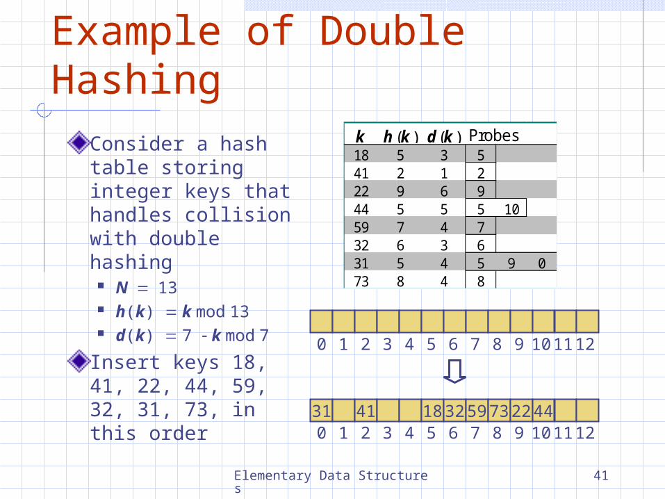
Consider a hash table storing integer keys that handles collision with double hashing
N13 h(k) k mod 13 d(k) 7 k mod 7
Insert keys 18, 41, 22, 44, 59, 32, 31, 73, in this order
Example of Double Hashing
0 1 2 3 4 5 6 7 8 9 10 11 12
31 41 183259732244 0 1 2 3 4 5 6 7 8 9 10 11 12
k h (k ) d (k ) Probes18 5 3 541 2 1 222 9 6 944 5 5 5 1059 7 4 732 6 3 631 5 4 5 9 073 8 4 8
Elementary Data Structures 42
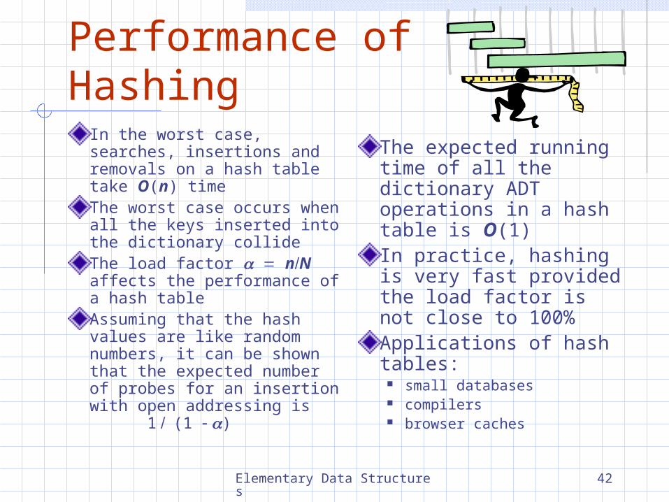
Performance of Hashing
In the worst case, searches, insertions and removals on a hash table take O(n) timeThe worst case occurs when all the keys inserted into the dictionary collideThe load factor nN affects the performance of a hash tableAssuming that the hash values are like random numbers, it can be shown that the expected number of probes for an insertion with open addressing is
1 (1 )
The expected running time of all the dictionary ADT operations in a hash table is O(1) In practice, hashing is very fast provided the load factor is not close to 100%Applications of hash tables:
small databases compilers browser caches
Elementary Data Structures 43
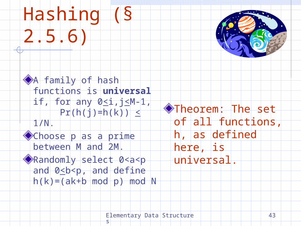
Universal Hashing (§ 2.5.6)
A family of hash functions is universal if, for any 0<i,j<M-1, Pr(h(j)=h(k)) < 1/N.Choose p as a prime between M and 2M.Randomly select 0<a<p and 0<b<p, and define h(k)=(ak+b mod p) mod N
Theorem: The set of all functions, h, as defined here, is universal.
Elementary Data Structures 44
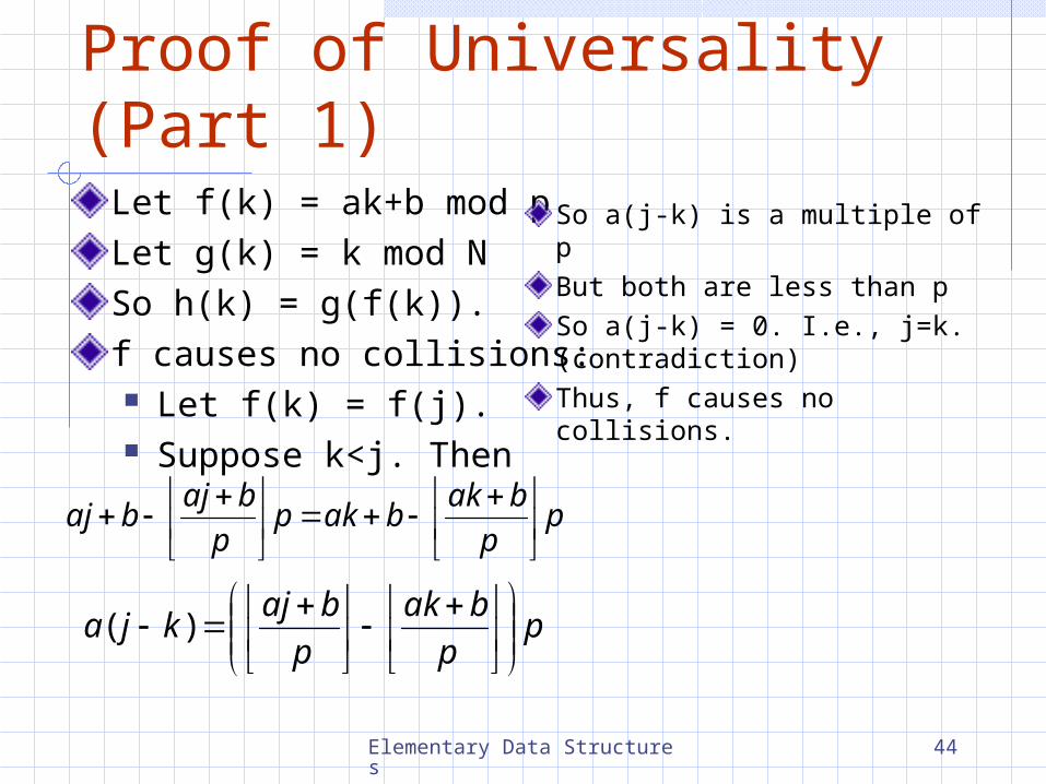
Proof of Universality (Part 1)
Let f(k) = ak+b mod pLet g(k) = k mod NSo h(k) = g(f(k)).f causes no collisions: Let f(k) = f(j). Suppose k<j. Then
pp
bakbakp
p
bajbaj
pp
bak
p
bajkja
)(
So a(j-k) is a multiple of pBut both are less than pSo a(j-k) = 0. I.e., j=k. (contradiction)Thus, f causes no collisions.
Elementary Data Structures 45
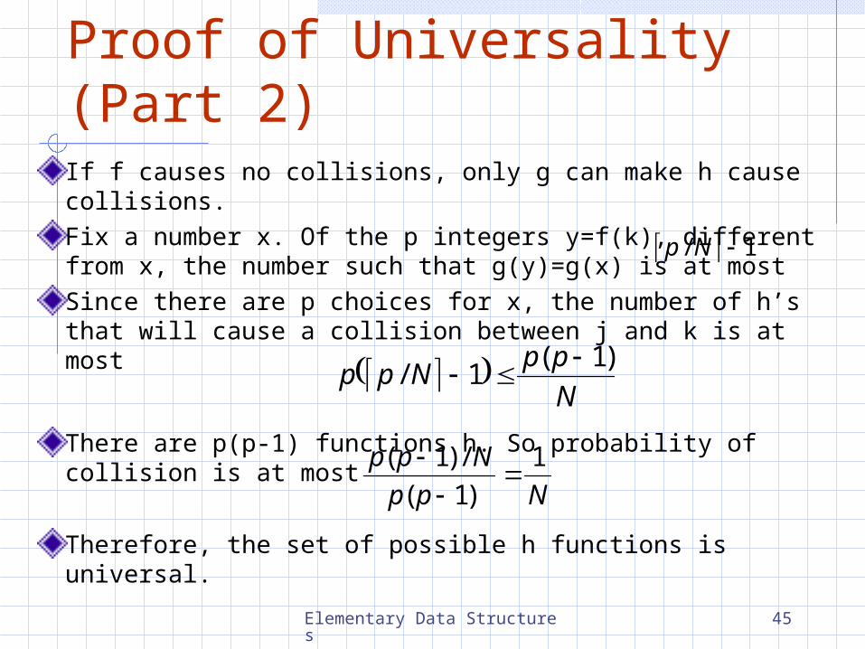
Proof of Universality (Part 2)If f causes no collisions, only g can make h cause collisions. Fix a number x. Of the p integers y=f(k), different from x, the number such that g(y)=g(x) is at most Since there are p choices for x, the number of h’s that will cause a collision between j and k is at most
There are p(p-1) functions h. So probability of collision is at most
Therefore, the set of possible h functions is universal.
1/ Np
N
ppNpp
)1(1/
Npp
Npp 1
)1(
/)1(