elemental: a new framework for distributed memory dense matrix · pdf fileelemental: a new...

Elemental: A New Framework for DistributedMemory Dense Matrix Computations

JACK POULSONThe University of Texas at AustinandBRYAN MARKERThe University of Texas at AustinandJEFF R. HAMMONDArgonne Leadership Computing FacilityandNICHOLS A. ROMEROArgonne Leadership Computing FacilityandROBERT A. VAN DE GEIJNThe University of Texas at Austin

Parallelizing dense matrix computations to distributed memory architectures is a well-studied

subject and generally considered to be among the best understood domains of parallel computing.Two packages, developed in the mid 1990s, still enjoy regular use: ScaLAPACK and PLAPACK.

With the advent of many-core architectures, which may very well take the shape of distributed

memory architectures within a single processor, these packages must be revisited since it willlikely not be practical to use MPI-based implementations. Thus, this is a good time to review

lessons learned since the introduction of these two packages and to propose a simple yet effectivealternative. Preliminary performance results show the new solution achieves competitive, if not

superior, performance on large clusters (i.e., on two racks of Blue Gene/P).

Categories and Subject Descriptors: G.4 [Mathematical Software]: —Efficiency

General Terms: Algorithms; Performance

Additional Key Words and Phrases: linear algebra, libraries, high-performance, parallel computing

Authors’ addresses: Jack Poulson, Institute for Computational Engineering and Sciences, The

University of Texas at Austin, Austin, TX 78712, [email protected]. Robert A. van de

Geijn and Bryan Marker, Department of Computer Science, The University of Texas at Austin,Austin, TX 78712, [email protected], [email protected]. Nichols A. Romero and Jeff R.Hammond, Argonne National Laboratory, 9700 South Cass Avenue, LCF/Building 240, Argonne,

IL 60439, {naromero, jhammond}@anl.gov.Permission to make digital/hard copy of all or part of this material without fee for personal

or classroom use provided that the copies are not made or distributed for profit or commercial

advantage, the ACM copyright/server notice, the title of the publication, and its date appear, andnotice is given that copying is by permission of the ACM, Inc. To copy otherwise, to republish,to post on servers, or to redistribute to lists requires prior specific permission and/or a fee.c© 20YY ACM 0098-3500/20YY/1200-0001 $5.00

ACM Transactions on Mathematical Software, Vol. V, No. N, Month 20YY, Pages 1–17.

2 · J. Poulson et al.

1. INTRODUCTION

With the advent of widely used commercial distributed memory architectures inthe late 1980s and early 1990s came the need to provide libraries for commonlyencountered computations. In response two packages, ScaLAPACK [Blackford et al.1997; Anderson et al. 1992; Dongarra and van de Geijn 1992; Anderson et al. 1992;Dongarra et al. 1994] and PLAPACK [Wu et al. 1996; Alpatov et al. 1997; van deGeijn 1997], were created in the mid-1990s, both of which provide a substantialpart of the functionality offered by the widely used LAPACK library [Andersonet al. 1999]. Both of these packages still enjoy loyal followings.

One of the authors of the present paper contributed to the early design of ScaLA-PACK and was the primarily architect of PLAPACK. This second package resultedfrom a desire to solve the programmability crisis that faced computational scientistsin the early days of massively parallel computing much like the programmabilityproblem that now faces us as multicore architectures evolve into many-core ar-chitectures. After major development on the PLAPACK project ceased around2000, many of the insights were brought back into the world of sequential andmulti-threaded architectures (including SMP and multicore), yielding the FLAMEproject [Gunnels et al. 2001], libflame library [Van Zee 2009], and SuperMatrixruntime system for scheduling dense linear algebra algorithms to multicore architec-tures [Chan et al. 2007; Quintana-Ort́ı et al. 2009]. With the advent of many-corearchitectures that may soon resemble “distributed memory clusters on a chip”,like the Intel 80-core network-on-a-chip terascale research processor [Mattson et al.2008] and the recently announced Intel Single-chip Cloud Computer (SCC) researchprocessor with 48 cores in one processor [Howard et al. 2010], the research comesfull circle: distributed memory libraries may need to be mapped to single-chipenvironments.

This seems an appropriate time to ask what we would do differently if we had tostart all over again building a distributed memory dense linear algebra library. Inthis paper we attempt to answer this question. This time the solution must trulysolve the programmability problem for this domain. It cannot compromise (much)on performance. It must be easy to retarget from a conventional cluster to a clusterwith hardware accelerators to a distributed memory cluster on a chip.

Both the ScaLAPACK and PLAPACK projects generated dozens of papers.Thus, this paper is merely the first in what we expect to be a series of papersthat together provide the new design. As such it is heavy on vision and somewhatlight on details. It is structured as follows: in Section 2, we review how matri-ces are distributed to the memories of a distributed memory architecture usingtwo-dimensional cyclic data distribution as well as the communications that areinherently encountered in parallel dense matrix computations. In Section 3, wediscuss how distributed memory code can be written so as to hide many of the in-dexing details that traditionally make libraries for distributed memory difficult todevelop and maintain. In Section 4, we show that elegance does not mean that per-formance must be sacrificed. Concluding remarks follow in the final section. Twoappendices are included. One describes the data distributions that underly Ele-mental in more detail while the other illustrates the parallel Cholesky factorizationthat is the model example used throughout the paper.ACM Transactions on Mathematical Software, Vol. V, No. N, Month 20YY.

Elemental · 3

Algorithm: A := Chol blk(A) Variant 3: down-looking

Partition A→ ATL ATR

? ABR

!where ATL is 0× 0

while m(ATL) < m(A) do

b = min(m(ABR), balg)

Repartition ATL ATR

? ABR

!→

0@ A00 A01 A02

? A11 A12

? ? A22

1Awhere A11 is b× b

A11 := Chol(A11)

A12 := A−H11 A12 (Trsm)

A22 := A22 −AH12A12 (Herk)

Continue with

ATL ATR

? ABR

!←

0@ A00 A01 A02

? A11 A12

? ? A22

1Aendwhile

Fig. 1. Blocked algorithms for computing the Cholesky factorization.

2. DISTRIBUTION AND COLLECTIVE COMMUNICATION

A key insight that underlies scalable dense linear algebra libraries for distributedmemory architectures is that the matrix must be distributed to MPI processes(processes hereafter) using a two-dimensional data distribution [Schreiber 1992;Stewart 1990; Hendrickson and Womble 1994]. The p processes in a distributedmemory architecture are logically viewed as a two-dimensional r× c mesh with p =rc. Subsequently, communication when implementing dense matrix computationscan be cast (almost) entirely in terms of collective communication within rows andcolumns of processes, with an occasional collective communication that involves allprocesses.

2.1 Motivating Example

In much of this paper, we will use the Cholesky factorization as our motivatingexample. An algorithm for this operation, known as the down-looking variant, thatlends itself well to parallelization is given in Figure 1.

2.2 Two-dimensional (block) cyclic distribution

Matrix A ∈ Rm×n is partitioned into blocks,

A =

A0,0 · · · A0,N−1

......

AM−1,0 · · · AM−1,N−1

,

ACM Transactions on Mathematical Software, Vol. V, No. N, Month 20YY.


where Ai,j is of a chosen (uniform) block size. A two-dimensional (Cartesian)block-cyclic matrix distribution assigns

A =

As,t As,t+c · · ·As+r,t As+r,t+c · · ·

......

to process (s, t).

2.3 ScaLAPACK

While in theory ScaLAPACK allows blocks Ai,j to be rectangular, in practice theyare chosen to be square. The design decisions that underly ScaLAPACK link thedistribution block size, bdistr, to the algorithmic block size, balg (e.g., the size ofblock A11 in Figure 1). Predicting the best distribution block size is often difficultbecause there is a tension between having block sizes that are large enough forlocal Basic Linear Algebra Subprogram (BLAS) [Dongarra et al. 1990] efficiency,yet small enough to avoid inefficiency due to load-imbalance.

The benefit of linking the two is that, for example, the A11 block in Figure 1is owned by a single process allowing it to be factored by one process. After thisfactoring, it only needs to be broadcast within the row of processes that ownsA12, and then those processes can independently perform their part of A12 :=U−H

11 A12 with local calls to trsm (meaning only c processes participate in thisoperations). Finally, A12 is duplicated within rows and columns of processes afterwhich A22 can be updated independently by each process. For some operations, thesimplicity of the distribution also allows for limited overlapping of communicationwith computation.

2.4 PLAPACK

In PLAPACK there is a notion of a vector distribution that induces the matrixdistribution [Edwards et al. 1995]. Vectors are subdivided into subvectors of lengthbdistr which are wrapped in a cyclic fashion to all processes. This vector distributionthen induces the distribution of columns and rows of a matrix to the mesh. Thenet effect is that the submatrices Ai,j are of size bdistr by r · bdistr. Algorithmsthat operate with the matrix are, as a result of this “unbalanced” distribution,mildly nonscalable in the sense that if the number of processes p gets large enough,efficiency will start to suffer even if the matrix is chosen to fill all of availablememory. In PLAPACK the distribution block size can be chosen to be small whilethe algorithmic block size can equal the block size that makes local computationefficient since the two block sizes are not linked.

The mild nonscalability of PLAPACK was the result of a conscious choice made tosimplify the implementation at a time when the number of processes was relativelysmall. There was always the intention to fix this eventually. The new packagedescribed in this paper is that fix, but it also incorporates other insights made inthe last decade.ACM Transactions on Mathematical Software, Vol. V, No. N, Month 20YY.

Elemental · 5

2.5 Elemental

In principle Elemental, like ScaLAPACK, can accomodate any distribution blocksize. Unlike ScaLAPACK and like PLAPACK, the distribution block size is notlinked to the algorithmic block size. Load balance is optimal when the distributionblock size is as small as possible, leading to the choice to initially (and possiblypermanently) only support bdistr = 1, unlike PLAPACK which is not implementedto be efficient when bdistr = 1. This choice also greatly simplifies routines that packand unpack messages before and after communication, since bdistr 6= 1 requirescareful attention to be paid to partial blocks, etc.

The insight to use bdistr = 1 is not new. On early distributed memory architec-tures, before the advent of cache-based processors that favor blocked algorithmslike the one in Figure 1, such an “elemental” distribution was the norm [Johnsson1987; Hendrickson and Womble 1994]. In [Hendrickson et al. 1999] it is noted that

“Block storage is not necessary for block algorithms and level 3 [BLAS] performance.Indeed, the use of block storage leads to a significant load imbalance when the block

size is large. This is not a concern on the Paragon, but may be problematic formachines requiring larger block sizes for optimal BLAS performance.”

Similarly, in [Strazdins 1998] it was experimentally shown that small distributionblock sizes that were independent of the algorithmic block size were beneficial. Thismay have been prophetic but has not become particularly relevant until recently.The reason is that the algorithmic block size used to be related to the (squareroot of the) size of the L1 cache [Whaley and Dongarra 1998], which was relativelysmall. Kazushige Goto [Goto and van de Geijn 2008] showed that higher perform-ing implementations should use the L2 cache for blocking, which means that thealgorithmic block size is now typically related to the (square root of the) size ofthe L2 cache. However, by the time this was discovered distributed memory archi-tectures had so much local memory that load balance could still be achieved forthe very large problem sizes that could be stored. More recently, the advent ofGPU accelerators push the block size higher yet, into the balg = 1000 range, so thatbdistr = balg will likely become problematic. Moreover, one path towards many-core(hundreds or even thousands of cores on one chip) is to create distributed memoryarchitectures on a chip [Howard et al. 2010]. In that scenario, the problem size willlikely not be huge due to an inability to have very large memories close to the chipand/or because the problems that will be targeted to those kinds of processors willbe relatively small.

To some the choice of bdistr = 1 may seem to be in contradition to conventionalwisdom that says that the more processor boundaries are encountered in the datapartitioning for distribution, the more often communication must occur. To explainwhy this is not necessarily true for dense matrix computations, consider the follow-ing observations regarding the parallelization of a blocked down-looking Choleskyfactorization:

—In the ScaLAPACK implementation, A11 is factored by a single process afterwhich it must be broadcast within the column of processes that owns it.

—If the matrix is distributed using bdistr = 1, then A11 can be gathered to allprocesses and factored redundantly. We note that, if communication cost is



ignored, this is as efficient as having a single process compute the factorizationwhile the other cores idle.

—If done correctly, an allgather to all processes is comparable in cost to the broad-cast of A11 performed by ScaLAPACK. (If the process mesh is p = r × c, underreasonable assumptions, the former requires log2(p) relatively short messageswhile the latter requires log2(r) such messages.)

The point is that, for the suboperation that factors A11, there is a small price to bepaid for switching to an elemental distribution. Next, consider the update of A12:

—In the ScaLAPACK implementation, A12 is updated by the c processes in theprocess row that owns it, requiring the broadcast of A11 within that row ofprocesses. Upon completion, the updated A12 is then broadcast within rows andcolumns of processes.

—If the matrix is distributed using bdistr = 1, then rows of A12 must be broughttogether so that they can be updated as part of A12 := U−H

11 A12. This can beimplemented as an all-to-all collective communication within columns (detailsof which are illustrated in Appendix B). After this, since A11 was redundantlyfactored by each process, the update A12 := U−H

11 A12 is shared among all pprocesses (again, details are illustrated in Appendix B).

Finally, consider the update of A22:

—An allgather within rows and columns then duplicates the elements of A12 (alsoillustrated in Appendix B) so that A22 can be updated in parallel; the ScaLA-PACK approach is similar but uses a broadcast rather than an allgather.

The point is that an elemental distribution requires different communications thatare comparable in cost to those incurred by ScaLAPACK while enhancing load-balance for operations like A12 := U−H

11 A12 and A22 := A22 −AH12A12.

3. PROGRAMMABILITY

A major concern when designing Elemental was that the same code should supportdistributed memory parallelism on both large-scale clusters and for many cores ona single chip. Thus, the software must be flexibly retargetable to both of theseextremes.

3.1 ScaLAPACK

The fundamental design decision behind ScaLAPACK can be found on the ScaLA-PACK webpage [ScaLAPACK 2010]:

“Like LAPACK, the ScaLAPACK routines are based on block-partitioned algorithms

in order to minimize the frequency of data movement between different levels of

the memory hierarchy. (For such machines, the memory hierarchy includes the off-processor memory of other processors, in addition to the hierarchy of registers, cache,

and local memory on each processor.) The fundamental building blocks of the ScaLA-

PACK library are distributed memory versions (PBLAS) of the Level 1, 2 and 3 BasicLinear Algebra Subprograms (BLAS), and a set of Basic Linear Algebra Communica-

tion Subprograms (BLACS) for communication tasks that arise frequently in parallel

linear algebra computations. In the ScaLAPACK routines, all interprocessor com-munication occurs within the PBLAS and the BLACS. One of the design goals of


Elemental · 7

SUBROUTINE PZPOTRF( UPLO, N, A, IA, JA, DESCA, INFO )

*

* -- ScaLAPACK routine (version 1.7) --

* University of Tennessee, Knoxville, Oak Ridge National Laboratory,

* and University of California, Berkeley.

* May 25, 2001

*

< deleted code >

*

DO 10 J = JN+1, JA+N-1, DESCA( NB_ )

JB = MIN( N-J+JA, DESCA( NB_ ) )

I = IA + J - JA

*

* Perform unblocked Cholesky factorization on JB block

*

CALL PZPOTF2( UPLO, JB, A, I, J, DESCA, INFO )

IF( INFO.NE.0 ) THEN

INFO = INFO + J - JA

GO TO 30

END IF

*

IF( J-JA+JB+1.LE.N ) THEN

*

* Form the row panel of U using the triangular solver

*

CALL PZTRSM( ’Left’, UPLO, ’Conjugate transpose’,

$ ’Non-Unit’, JB, N-J-JB+JA, CONE, A, I, J,

$ DESCA, A, I, J+JB, DESCA )

*

* Update the trailing matrix, A = A - U’*U

*

CALL PZHERK( UPLO, ’Conjugate transpose’, N-J-JB+JA, JB,

$ -ONE, A, I, J+JB, DESCA, ONE, A, I+JB,

$ J+JB, DESCA )

END IF

10 CONTINUE

< deleted code >

Fig. 2. Excerpt from ScaLAPACK Cholesky factorization. Parallelism is hidden inside calls toparallel implementations of BLAS operations, which limits the possiblity of combining commu-nication required for individual such operations. (The header refers to ScaLAPACK 1.7 but this

excerpt is from the code in the latest release, ScaLAPACK 1.8. dated April 5 2007.)

ScaLAPACK was to have the ScaLAPACK routines resemble their LAPACK equiv-

alents as much as possible.”

In Figure 2 we show the ScaLAPACK Cholesky factorization routine. A readerwho is familiar with the LAPACK Cholesky factorization will notice the similarityof coding style.

3.2 PLAPACK

As mentioned PLAPACK already supports balg 6= bdistr. While bdistr = 1 is sup-ported, the communication layer of PLAPACK would need to be rewritten and thenonscalability of the underlying distribution would need to be fixed.

Since the inception of PLAPACK, additional insights into solutions to the pro-ACM Transactions on Mathematical Software, Vol. V, No. N, Month 20YY.


grammability problem for dense matrix computations were exposed as part of theFLAME project and incorporated into the libflame library. To also incorporateall those insights, a complete rewrite of PLAPACK made more sense, yielding El-emental.

3.3 Elemental

Elemental goes one step beyond libflame in that it is coded in C++1. Otherthan this small detail, the coding style resembles that used by libflame. Like itspredecessors PLAPACK and libflame, it hides the details of matrices and vectorswithin objects. As a result, much of the indexing clutter that exists in LAPACKand ScaLAPACK code disappears, leading to much easier to develop and maintaincode.

Let us examine how the code in Figure 3 implements the algorithm described inSection 2.5.

—The tracking of submatrices in Figure 1 translates toPartitionDownDiagonal( A, ATL, ATR,

ABL, ABR, 0 );

while( ABR.Height() > 0 )

{

RepartitionDownDiagonal( ATL, /**/ ATR, A00, /**/ A01, A02,

/*************/ /******************/

/**/ A10, /**/ A11, A12,

ABL, /**/ ABR, A20, /**/ A21, A22 );

[...]

SlidePartitionDownDiagonal( ATL, /**/ ATR, A00, A01, /**/ A02,

/**/ A10, A11, /**/ A12,

/*************/ /******************/

ABL, /**/ ABR, A20, A21, /**/ A22 );

}

—Redistributing A11 so that all processes have a copy is achieved byDistMatrix<T,Star,Star> A11_Star_Star(g);

which indicates that A11 Star Star describes a matrix replicated on all processes,and

A11_Star_Star = A11;

lapack::internal::LocalChol( Upper, A11_Star_Star );

A11 = A11_Star_Star;

which performs an allgather of the data, has every process redundantly factor thematrix, and then locally substitutes the new values into the distributed matrix.

—The parallel computation of A12 := U−H11 A12 is accomplished by first constructing

an object for holding a temporary distribution of A12,DistMatrix<T,Star,VR> A12_Star_VR(g);

which describes what in PLAPACK would have been called a multivector distri-bution, followed by

A12_Star_VR = A12;

blas::internal::LocalTrsm

( Left, Upper, ConjugateTranspose, NonUnit,

(T)1, A11_Star_Star, A12_Star_VR );

1In the future, the library will be accessible from Fortran or C via wrappers.


Elemental · 9

template<typename T>

void CholU( DistMatrix<T,MC,MR>& A )

{

const Grid& g = A.GetGrid();

DistMatrix<T,MC,MR> ATL(g), ATR(g), A00(g), A01(g), A02(g),

ABL(g), ABR(g), A10(g), A11(g), A12(g),

A20(g), A21(g), A22(g);

DistMatrix<T,Star,Star> A11_Star_Star(g);

DistMatrix<T,Star,VR > A12_Star_VR(g);

DistMatrix<T,Star,MC > A12_Star_MC(g);

DistMatrix<T,Star,MR > A12_Star_MR(g);

PartitionDownDiagonal( A, ATL, ATR,

ABL, ABR, 0 );

while( ABR.Height() > 0 )

{

RepartitionDownDiagonal( ATL, /**/ ATR, A00, /**/ A01, A02,

/*************/ /******************/

/**/ A10, /**/ A11, A12,

ABL, /**/ ABR, A20, /**/ A21, A22 );

A12_Star_MC.AlignWith( A22 );

A12_Star_MR.AlignWith( A22 );

A12_Star_VR.AlignWith( A22 );

//--------------------------------------------------------------//


lapack::internal::LocalChol( Upper, A11_Star_Star );

A11 = A11_Star_Star;

A12_Star_VR = A12;

blas::internal::LocalTrsm

( Left, Upper, ConjugateTranspose, NonUnit,

(T)1, A11_Star_Star, A12_Star_VR );

A12_Star_MC = A12_Star_VR;

A12_Star_MR = A12_Star_VR;

blas::internal::LocalTriangularRankK

( Upper, ConjugateTranspose,

(T)-1, A12_Star_MC, A12_Star_MR, (T)1, A22 );

A12 = A12_Star_MR;

//--------------------------------------------------------------//

A12_Star_MC.FreeAlignments();

A12_Star_MR.FreeAlignments();

A12_Star_VR.FreeAlignments();

SlidePartitionDownDiagonal( ATL, /**/ ATR, A00, A01, /**/ A02,

/**/ A10, A11, /**/ A12,

/*************/ /******************/

ABL, /**/ ABR, A20, A21, /**/ A22 );

}

}

Fig. 3. Elemental upper-triangular variant 3 Cholesky factorization.



which redistributes the data via an all-to-all communication within columns andperforms the local portion of the update A12 := A−H

11 A12 (Trsm).—The subsequent redistribution of A12 so that A22 := A22−AH

12A12 is accomplishedby first constructing two temporary distributions,

DistMatrix<T,Star,MC> A12_Star_MC(g);

DistMatrix<T,Star,MR> A12_Star_MR(g);

which describe the two distributions needed to make the update of A22 local.The redistributions themselves are accomplished by the commands

A12_Star_VR = A12;

A12_Star_MC = A12_Star_VR;

A12_Star_MR = A12_Star_VR;

which perform a permutation of data among all processes, an allgather of datawithin rows, and an allgather of data within columns, respectively. (Details ofhow and why these communications are performed will be given in a future, morecomprehensive paper.) The local update of A22 is accomplished by

blas::internal::LocalTriangularRankK

( Upper, ConjugateTranspose,

(T)-1, A12_Star_MC, A12_Star_MR,(T)1, A22 );

—Finally, the updated A12 is placed back into the distributed matrix, withoutrequiring any communication, by the command

A12 = A12_Star_MR;

The point is that the Elemental framework allows the partitioning, distributions,communications, and local computations to be elegantly captured in code. Thedata movements that are incurred are further illustrated in Appendix B while anexplanation of the data distributions is given in Appendix A.

4. PERFORMANCE EXPERIMENTS

The scientific computing community has always been willing to give up programma-bility if it means attaining better performance. In this section, we give preliminaryperformance numbers that suggest that a focus on programmability does not needto come at the cost of performance.

4.1 Platform details

The performance experiments were carried out on Argonne National Laboratory’sIBM Blue Gene/P architecture. Each compute node consists of four 850 MHz Pow-erPC 450 processors for a combined theoretical peak performance of 13.6 GFlopsin double-precision arithmetic per node. Nodes are interconnected by a three-dimensional torus topology and a collective network that each support a per nodebidirectional bandwidth of 2.55 GB/s. Our experiments were performed on tworacks (2048 compute nodes, or 8192 cores), which have an aggregate theoreticalpeak of just over 27 TFlops For this configuration the X, Y , and Z dimensionsof the torus are 8, 8, and 32, respectively. The optimal decomposition into a two-dimensional topology was almost always Z × (X,Y ), which was used for the belowexperiments.

We compare the performance of a preliminary version of Elemental ported toBlue Gene/P (Elemental-BG/P) with the latest release of ScaLAPACK availablefrom netlib (Release 1.8). Since experiments showed that ScaLAPACK performsACM Transactions on Mathematical Software, Vol. V, No. N, Month 20YY.

Elemental · 11

worse in SMP mode, its performance results are reported with one MPI process percore with local computation performed by calls to BLAS provided by IBM’s serialESSL library. Elemental-BG/P performance is reported with one MPI process percore and with one MPI process per node (SMP mode). The shared memory par-allelism simply consists of using IBM’s threaded ESSL BLAS library and addingsimple OpenMP directives for parallelizing the packing and unpacking steps sur-rounding MPI calls. Both packages were tested for all block sizes in the range32, 64, 96, ..., 256, with only the best-performing block size for each problem size re-ported in the graphs. All reported computations were performed in double-precision(64-bit) arithmetic.

4.2 Operations

Solution of the Hermitian generalized eigenvalue problem, given by Ax = λBxwhere A and B are known, A is Hermitian, and B is Hermitian positive-definite,is of importance to the coauthors of this paper from Argonne National Lab. Thisoperations is typically broken down into six steps:

—Cholesky factorization. B → LLH where L is lower triangular.

—Reduction of the generalized problem to Hermitian standard form.The transformation C := L−1AL−H .

—Householder reduction to tridiagonal form. Computes unitary Q (as asequence of Householder transformations) so that T = QCQH is tridiagonal.

—Spectral decomposition of a tridiagonal matrix. Computes unitary V suchthat T = V DV H where D is diagonal. This part of the problem is not includedin the performance experiments. It could employ, for example, the PMRRRalgorithms [Bientinesi et al. 2005].

—Back transformation. This operations computes Z = QHV by applying theHouseholder transformations that represent Q to V .

—Solution of a triangular system of equations with multiple right-handsides. Now A(L−HZ) = C(L−HZ) and hence X = L−HZ equal the desiredgeneralized eigenvectors. This requires the solution of the triangular system ofequations LX = Z.

Since complex arithmetic requires four times as many floating point operations,we tuned and measured performance for double-precision real matrices. The repre-sented performance is qualitatively representative of that observed for the complexcase. To further reduce the time required for collecting data we limited the largestproblem size for which performance is reported to 100, 000 × 100, 000, which re-quires less than one percent of the available main memory of the 2048 nodes foreach distributed matrix.

4.3 Results

The point of this section is to show that preliminary experience with Elementalsupports the claim that it provides a solution to the programmability problemwithout sacrificing performance. Potential users of ScaLAPACK and Elementalare encouraged to perform and report their own comparisons.



0 0.2 0.4 0.6 0.8 1

·105

0

10

20

Dimension

TF

lop

s

Elemental-BG/P

Elemental-BG/P SMP

ScaLAPACK

0 0.2 0.4 0.6 0.8 1

·105

100

101

102

Dimension

Tim

e[s

econ

ds]

Elemental-BG/P

Elemental-BG/P SMP

ScaLAPACK

Fig. 4. Real double-precision Cholesky factorization on 8192 cores.

0 0.2 0.4 0.6 0.8 1

·105

0

10

20

Dimension

TF

lop

s

Elemental-BG/P

Elemental-BG/P SMP

ScaLAPACK

0 0.2 0.4 0.6 0.8 1

·105

100

101

102

103

Dimension

Tim

e[s

econ

ds]

Elemental-BG/P

Elemental-BG/P SMP

ScaLAPACK

Fig. 5. Real double-precision reduction of generalized eigenvalue problem to symmetric standard

form on 8192 cores.

0 0.2 0.4 0.6 0.8 1

·105

0

10

20

Dimension

TF

lop

s

Elemental-BG/P

Elemental-BG/P SMP

ScaLAPACK

0 0.2 0.4 0.6 0.8 1

·105

101

102

103

Dimension

Tim

e[s

econ

ds]

Elemental-BG/P

Elemental-BG/P SMP

ScaLAPACK

Fig. 6. Real double-precision Householder tridiagonalization on 8192 cores.


Elemental · 13

0 0.2 0.4 0.6 0.8 1

·105

0

10

20

Dimension

TF

lop

sElemental-BG/P

Elemental-BG/P SMP

ScaLAPACK

0 0.2 0.4 0.6 0.8 1

·105

100

101

102

Dimension

Tim

e[s

econ

ds]

Elemental-BG/P

Elemental-BG/P SMP

ScaLAPACK

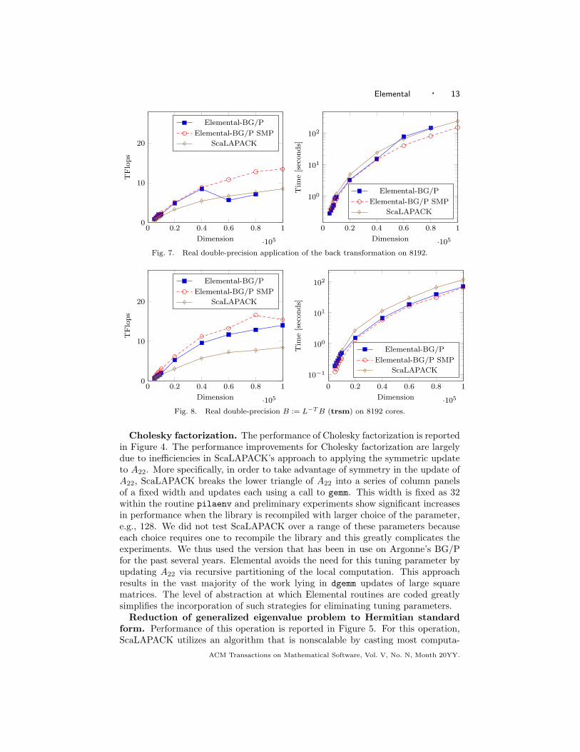
Fig. 7. Real double-precision application of the back transformation on 8192.

0 0.2 0.4 0.6 0.8 1

·105

0

10

20

Dimension

TF

lop

s

Elemental-BG/P

Elemental-BG/P SMP

ScaLAPACK

0 0.2 0.4 0.6 0.8 1

·105

10−1

100

101

102

Dimension

Tim

e[s

econ

ds]

Elemental-BG/P

Elemental-BG/P SMP

ScaLAPACK

Fig. 8. Real double-precision B := L−TB (trsm) on 8192 cores.

Cholesky factorization. The performance of Cholesky factorization is reportedin Figure 4. The performance improvements for Cholesky factorization are largelydue to inefficiencies in ScaLAPACK’s approach to applying the symmetric updateto A22. More specifically, in order to take advantage of symmetry in the update ofA22, ScaLAPACK breaks the lower triangle of A22 into a series of column panelsof a fixed width and updates each using a call to gemm. This width is fixed as 32within the routine pilaenv and preliminary experiments show significant increasesin performance when the library is recompiled with larger choice of the parameter,e.g., 128. We did not test ScaLAPACK over a range of these parameters becauseeach choice requires one to recompile the library and this greatly complicates theexperiments. We thus used the version that has been in use on Argonne’s BG/Pfor the past several years. Elemental avoids the need for this tuning parameter byupdating A22 via recursive partitioning of the local computation. This approachresults in the vast majority of the work lying in dgemm updates of large squarematrices. The level of abstraction at which Elemental routines are coded greatlysimplifies the incorporation of such strategies for eliminating tuning parameters.

Reduction of generalized eigenvalue problem to Hermitian standardform. Performance of this operation is reported in Figure 5. For this operation,ScaLAPACK utilizes an algorithm that is nonscalable by casting most computa-



tion in terms of the parallel solution of a triangular system with multiple right-handsides (trsm) and parallel triangular matrix-matrix multiplication (trmm). These op-erations work with only a narrow panel of right-hand sides (with width equal tothe block size), which greatly limits the opportunity for parallelism. By contrastElemental uses a new algorithm [Poulson 2009] that casts most computation interms of rank-k updates, which are easily parallelizable. The vast performance im-provement observed in this routine can be entirely attributed to the new algorithmavoiding unscalable updates.

Householder reduction to tridiagonal form. In Figure 6, we report theperformance for the reduction to tridiagonal form. This operation is the most timeconsuming step towards finding all eigenvalues and eigenvectors of a symmetric orHermitian matrix. Neither package attains the same level of performance as do theother operations. The reason for this is that a substantial part of the computation isin a (local) matrix-vector multiplication, which is inherently constrained by memorybandwidth. The algorithms used by both packages are essentially the same.

Back transformation. This operation requires the Householder transforma-tions that form Q to be applied to the eigenvectors of the tridiagonal matrix T .Our parallel implementation employs block UT transforms [Joffrain et al. 2006] inorder to cast most of the computation in terms of efficient matrix-matrix multipli-cations. Results are reported in Figure 7. The dramatic drop in the performancecurve for Elemental is due to a large drop in efficiency of IBM’s MPI Reduce scatterimplementation over the (Z, T ) subtori once the message sizes are larger than a par-ticular value. We are in the process of working out the problem with IBM.

Solution of a triangular system of equations with multiple right-handsides. Parallelization of this operation was first published in [Chtchelkanova et al.1997] and it is part of ScaLAPACK’s Parallel BLAS (PBLAS). Results are reportedin Figure 7.

4.4 Discussion

Both ScaLAPACK and Elemental have considerably large searchspaces of tuningparameters, so our experiments always included testing both packages over the samelarge range of blocksizes, process grid dimensions, and matrix sizes. Unfortunatelyan exhaustive search is infeasible, so we make no claims that we have found theoptimal parameters for each package. However, we believe that our experimentswere sufficiently detailed for qualitative comparison. In particular, we would like topoint out that the factor of 20 performance improvement observed in the reductionof the generalized eigenvalue problem resulted from a smarter algorithm ratherthan a smarter implementation; all other performance differences are insignificantin comparison.

5. CONCLUSION

The point of this paper is to demonstrate that, for the domain of dense linearalgebra libraries, neither abstraction nor elegance needs to stand in the way of per-formance, even on distributed memory architectures. Therefore, it is time for thecommunity to embrace notations, techniques, algorithms, abstractions, and APIsthat help solve the programmability problem in preparation for exascale comput-ing, rather than remaining fixated on performance at the expense of sanity. OnACM Transactions on Mathematical Software, Vol. V, No. N, Month 20YY.

Elemental · 15

future architectures that also incorporate GPUs, the effect of programmability onperformance is expected to be even more pronounced.

As of this writing, Elemental supports the following functionality, for both realand complex datatype:

—All level-3 BLAS.

—All three (one-sided) matrix factorizations: LU with partial pivoting, Cholesky,and QR factorization.

—All operations for computing the inverse of a symmetric/Hermitian positive-definite matrix.

—All operations for computing the solution of the generalized symmetric/Hermitianpositive-definite eigenvalue problem, with the exception of the parallel solutionof the symmetric tridiagonal eigensolver.

Soon, we expect to have functionality that rivals that of ScaLAPACK, with thepossible exception of solvers for the nonsymmetric eigenvalue problem.

We envision a string of additional papers in the near future. In Appendix A,we hint at a general set-based notation for describing the data distributions thatunderly Elemental. The key insight is that relations between sets, via the unionoperator, that link the different destributions dictate the communications that arerequired for parallelization. A full paper on this topic is being written. Anotherpaper will give details regarding the parallel computation of the solution of thegeneralized Hermitian eigenvalue problem.

As mentioned in the abstract and introduction, a major reason for creating a newdistributed memory dense matrix library and framework is the arrival of many-corearchitectures that can be viewed as clusters on a single chip, like the SCC archi-tecture. The Elemental library has already been ported to the SCC processor byreplacing the MPI collective communication library with calls to a custom collectivecommunication library for that architecture. The results of that experiment willalso be reported in a future publication.

Availability

The Elemental package is available at http://code.google.com/p/elemental andits port to Blue Gene/P at http://code.google.com/p/elemental-bgp.

Acknowledgements

This research was partially sponsored by NSF grants OCI-0850750 and CCF-0917167,grants from Microsoft, an unrestricted grant from Intel, and a fellowship from theInstitute of Computational Engineering and Sciences. Jack Poulson was also par-tially supported by a fellowship from the Institute of Computational Engineeringand Sciences, and Bryan Marker was partially supported by a Sandia National Lab-oratory fellowship. This research used resources of the Argonne Leadership Com-puting Facility at Argonne National Laboratory, which is supported by the Officeof Science of the U.S. Department of Energy under contract DE-AC02-06CH11357;early experiments were performed on the Texas Advanced Computing Center’sRanger Supercomputer.



Any opinions, findings and conclusions or recommendations expressed in thismaterial are those of the author(s) and do not necessarily reflect the views of theNational Science Foundation (NSF).

We would like to thank John Lewis (Cray) and John Gunnels (IBM T.J. WatsonResearch Center) for there constructive comments on this work and Brian Smith(IBM Rochester) for his help in eliminating performance problems in Blue Gene/P’scollective communication library.

REFERENCES

Alpatov, P., Baker, G., Edwards, C., Gunnels, J., Morrow, G., Overfelt, J., van de Geijn,R., and Wu, Y.-J. J. 1997. PLAPACK: Parallel linear algebra package – design overview. In

Proceedings of SC97.

Anderson, E., Bai, Z., Bischof, C., Blackford, L. S., Demmel, J., Dongarra, J. J., Croz,J. D., Hammarling, S., Greenbaum, A., McKenney, A., and Sorensen, D. 1999. LAPACK

Users’ guide (third ed.). Society for Industrial and Applied Mathematics, Philadelphia, PA,

USA.

Anderson, E., Benzoni, A., Dongarra, J., Moulton, S., Ostrouchov, S., Tourancheau, B.,and van de Geijn, R. 1992. Lapack for distributed memory architectures: Progress report.

In Proceedings of the Fifth SIAM Conference on Parallel Processing for Scientific Computing.

SIAM, Philadelphia, 625–630.

Bientinesi, P., Dhillon, I. S., and van de Geijn, R. A. 2005. A parallel eigensolver for dense

symmetric matrices based on multiple relatively robust representations. SIAM Journal on

Scientific Computing 27, 1, 43–66.

Blackford, L. S., Choi, J., Cleary, A., D’Azevedo, E., Demmel, J., Dhillon, I., Dongarra,J., Hammarling, S., Henry, G., Petitet, A., Stanley, K., Walker, D., and Whaley, R. C.

1997. ScaLAPACK Users’ Guide. SIAM.

Chan, E., Quintana-Ort́ı, E., Quintana-Ort́ı, G., and van de Geijn, R. 2007. SuperMatrixout-of-order scheduling of matrix operations for SMP and multi-core architectures. In SPAA

’07: Proceedings of the Nineteenth ACM Symposium on Parallelism in Algorithms and Archi-

tectures. 116–126.

Chtchelkanova, A., Gunnels, J., Morrow, G., Overfelt, J., and van de Geijn, R. A. 1997.Parallel implementation of BLAS: General techniques for level 3 BLAS. Concurrency: Practice

and Experience 9, 9 (Sept.), 837–857.

Dongarra, J. and van de Geijn, R. 1992. Reduction to condensed form on distributed memoryarchitectures. Parallel Computing 18, 973–982.

Dongarra, J., van de Geijn, R., and Walker, D. 1994. Scalability issues affecting the design

of a dense linear algebra library. J. Parallel Distrib. Comput. 22, 3 (Sept.).

Dongarra, J. J., Du Croz, J., Hammarling, S., and Duff, I. 1990. A set of level 3 basic linearalgebra subprograms. ACM Trans. Math. Soft. 16, 1 (March), 1–17.

Edwards, C., Geng, P., Patra, A., and van de Geijn, R. 1995. Parallel matrix distributions:

have we been doing it all wrong? Tech. Rep. TR-95-40, Department of Computer Sciences, The

University of Texas at Austin.

Goto, K. and van de Geijn, R. A. 2008. Anatomy of high-performance matrix multiplication.

ACM Trans. Math. Soft. 34, 3: Article 12, 25 pages (May).

Gunnels, J. A., Gustavson, F. G., Henry, G. M., and van de Geijn, R. A. 2001. FLAME: For-

mal Linear Algebra Methods Environment. ACM Transactions on Mathematical Software 27, 4(December), 422–455.

Hendrickson, B., Jessup, E., and Smith, C. 1999. Toward an efficient parallel eigensolver for

dense symmetric matrices. SIAM J. Sci. Comput. 20, 3, 1132–1154.

Hendrickson, B. A. and Womble, D. E. 1994. The torus-wrap mapping for dense matrixcalculations on massively parallel computers. SIAM J. Sci. Stat. Comput. 15, 5, 1201–1226.


Elemental · 17

Howard, J., Dighe, S., Hoskote, Y., Vangal, S., Finan, D., Ruhl, G., Jenkins, D., Wilson,

H., Borkar, N., Schrom, G., Pailet, F., Jain, S., Jacob, T., Yada, S., Marella, S., Sali-hundam, P., Erraguntla, V., Konow, M., Riepen, M., Droege, G., Lindemann, J., Gries,

M., Apel, T., Henriss, K., Lund-Larsen, T., Steibl, S., Borkar, S., De1, V., Wijngaart,

R. V. D., and Mattson, T. 2010. A 48-core IA-32 message-passing processor with DVFS in45nm CMOS. In Proceedings of the International Solid-State Circuits Conference.

Joffrain, T., Low, T. M., Quintana-Ort́ı, E. S., van de Geijn, R., and Van Zee, F. G.

2006. Accumulating householder transformations, revisited. ACM Trans. Math. Softw. 32, 2,169–179.

Johnsson, S. L. 1987. Communication efficient basic linear algebra computations on hypercube

architectures. J. of Par. Distr. Comput. 4, 133–172.

Mattson, T. G., Van der Wijngaart, R., and Frumkin, M. 2008. Programming the intel

80-core network-on-a-chip terascale processor. In SC’08: Proceedings of the 2008 ACM/IEEEconference on Supercomputing. IEEE Press, Piscataway, NJ, USA, 1–11.

Poulson, J. 2009. Formalized parallel dense linear algebra and its application to the generalized

eigenvalue problem. M.S. thesis, Department of Aerospace Engineering, The University ofTexas.

Quintana-Ort́ı, G., Quintana-Ort́ı, E. S., van de Geijn, R. A., Van Zee, F. G., and Chan,

E. 2009. Programming matrix algorithms-by-blocks for thread-level parallelism. ACM Trans-

actions on Mathematical Software 36, 3 (July), 14:1–14:26.

ScaLAPACK 2010. Home Page. http://www.netlib.org/scalapack/scalapack_home.html.

Schreiber, R. 1992. Scalability of sparse direct solvers. Graph Theory and Sparse Matrix

Computations 56.

Stewart, G. 1990. Communication and matrix computations on large message passing systems.

Parallel Computing 16, 27–40.

Strazdins, P. E. 1998. Optimal load balancing techniques for block-cyclic decompositions for

matrix factorization. In Proceedings of PDCN’98 2nd International Conference on Parallel

and Distributed Computing and Networks.

van de Geijn, R. A. 1997. Using PLAPACK: Parallel Linear Algebra Package. The MIT Press.

Van Zee, F. G. 2009. libflame: The Complete Reference. www.lulu.com.

Whaley, R. C. and Dongarra, J. J. 1998. Automatically tuned linear algebra software. In

Proceedings of SC’98.

Wu, Y.-J. J., Alpatov, P. A., Bischof, C., and van de Geijn, R. A. 1996. A parallel imple-

mentation of symmetric band reduction using PLAPACK. In Proceedings of Scalable ParallelLibrary Conference, Mississippi State University. PRISM Working Note 35.

Received Month Year; revised Month Year; accepted Month Year



Note to the referees: We envision Appendix A and B as electronic appendicesso that color has meaning.

A. ELEMENTAL DISTRIBUTION DETAILS

In this appendix, we describe the basics of the distribution used by Elemental andhow it facilitates parallel Cholesky factorization.

In our discussion, we assume that the p processes from a (logical) r × c meshwith p = rc. We let A ∈ Rm×n equal

A =

α00 α01 · · · α0(n−1)

α10 α11 · · · α1(n−1)

......

. . ....

α(m−1)0 α(m−1)1 · · · α(m−1)(n−1)

.

A.1 Distribution A(MC ,MR)

The basic elemental matrix distribution of matrix A assigns to process (s, t) of anr × c mesh of processes the submatrix

A =

αs,t αs,t+c · · ·αs+r,t αs+r,t+c · · ·

......

.

In Matlab notation (starting indexing at zero) this means that process (s, t) ownssubmatrix αs:r:m,t:c:n. We will denote this distribution by A(MC ,MR) whereMC

can be thought of as the set of sets of integers {Ms,tC } with s = 0, . . . , r − 1 and

t = 0, . . . , c− 1. The sets {Ms,tC } and {Ms,t

R } indicate two “filters” that determinethe row and column indices, respectively, of the matrix that are assigned to process(s, t). Figure 9 illustrates this.

The MC and MR are meant to represent a partitioning of the natural numbers(which include zero since we are computer scientists) into r and c nonoverlappingsubsets, respectively: MC =

(M0

C ,M1C , . . . ,M

r−1C

)andMR =

(M0

R,M1R, . . . ,M

c−1R

).

Now, A(Ms,tC ,Ms,t

R ) represents the submatrix of A that is formed by only choos-ing the row indices from Ms,t

C and column indices from Ms,tR . The notation

A(MC ,MR) is meant to indicate the distribution that assigns A(Ms,tC ,Ms,t

R ) toeach process (s, t).

While this notation captures a broad family of distributions, in the elementaldistributionMs

C = {s, s+ r, s+ 2r, . . .} andMtR = {t, t+ c, t+ 2c, . . .} creating the

desired round-robin distribution in Figure 9.

A.2 Distribution A(VC , ?)

This second distribution can be described as follows: The processes still forms anr × c mesh, but now the processes are numbered in column-major order: process(0, 0) is process 0. process (1, 0) is process 1, etc. process u in this numberingis assigned elements αu,∗, αu+p,∗, . . . where ∗ indicates all valid column indices.Another way of describing this is that the processes are now viewed as forminga one-dimensional array and rows of the matrix are wrapped onto this array in around-robin fashion. This is illustrated in Figure 10.ACM Transactions on Mathematical Software, Vol. V, No. N, Month 20YY.

Elemental · 19

Process (0,0) Process (0,1) Process (0,2)α0,0 α0,3 α0,6 · · · α0,1 α0,4 α0,7 · · · α0,2 α0,5 α0,8 · · ·α3,0 α3,3 α3,6 · · · α3,1 α3,4 α3,7 · · · α3,2 α3,5 α3,8 · · ·α6,0 α6,3 α6,6 · · · α6,1 α6,4 α6,7 · · · α6,2 α6,5 α6,8 · · ·

......

.... . .

......

.... . .

......

.... . .

Process (1,0) Process (1,1) Process (1,2)

α1,0 α1,3 α1,6 · · · α1,1 α1,4 α1,7 · · · α1,2 α1,5 α1,8 · · ·α4,0 α4,3 α4,6 · · · α4,1 α4,4 α4,7 · · · α4,2 α4,5 α4,8 · · ·α7,0 α7,3 α7,6 · · · α7,1 α7,4 α7,7 · · · α7,2 α7,5 α7,8 · · ·

......

.... . .

......

.... . .

......

.... . .

Process (2,0) Process (2,1) Process (2r,2)


......

.... . .

......

.... . .

......

.... . .

Fig. 9. Illustration of distribution A(MC ,MR) where r = c = 3, Ms,tC = {s, s + r, . . .}, and

Ms,tR = {t, t+ c, . . .}. Here the (s, t) tile represents process (s, t).

Process 0 Process 3 Process 6


......

.... . .

......

.... . .

......

.... . .



......

.... . .

......

.... . .

......

.... . .

Process 2 Process 5 Process 8α2,0 α2,1 α2,2 · · · α5,0 α5,1 α5,2 · · · α8,0 α8,1 α8,2 · · ·α11,0 α11,1 α11,2 · · · α14,0 α14,1 α14,2 · · · α17,0 α17,1 α17,2 · · ·α20,0 α20,1 α20,2 · · · α23,0 α23,1 α23,2 · · · α26,0 α26,1 α26,2 · · ·

......

.... . .

......

.... . .

......

.... . .

Fig. 10. Illustration of distribution A(VC , ∗) where r = c = 3 and Vs,tC = {u, u + p, . . .}, with

u = (formula).

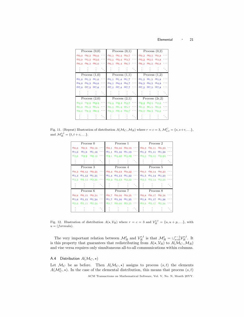
What is important is that it is very easy to redistribute from A(MC ,MR) toA(VC , ?). Focus on the first row of matrix A in Figures 9 and 10. The elementsof row 0 of A in Figure 9 need to be gathered within the first row of processesto process (0, 0) so that it becomes distributed as in Figure 10. Similarly, theelements of row 1 of A need to be gathered to process (1, 0). A careful comparisonof the two figures shows that all-to-all communications within rows of processes willredistribute A(MC ,MR) to A(VC , ?).

The VC represents a partitioning of the natural numbers into a 2D array of pACM Transactions on Mathematical Software, Vol. V, No. N, Month 20YY.


nonoverlapping subsets:

VC =

V0,0C , . . . ,V0,c−1

C...

Vr−1,0C , . . . ,Vr−1,c−1

C

Now, A(Vs,t

C , ?) represents the submatrix of A that is formed by only choosing therows with indices found in Vs,t

C . The notation A(VC , ?) is meant to indicate thedistribution that assigns A(Vs,t

C , ?) to each process (s, t). In the case where A is avector, x, the notation x(VC) can be used.

This notation also captures a broad family of distributions. In the elementaldistribution Vs,t

C = {u, u+p, u+2p, . . .}, where u = s+rt, creating the round-robindistribution in Figure 10.

The very important relation between MsC and Vs,t

C is that MsC = ∪c−1

t=0Vs,tC . It

is this property that guarantees that redistributing from A(VC , ?) to A(MC ,MR)and vise versa requires only simultaneous all-to-all communications within rows.

A.3 Distribution A(?,VR)

This distribution can be similarly described: The processes still forms an r×c mesh,but now the processes are numbered in row-major order: process (0, 0) is process0. process (0, 1) is process 1, etc. process u in this numbering is assigned elementsα∗,u, α∗,u+p, . . . where ∗ indicates all valid row indices. Another way of describingthis is that the processes are now viewed as forming a one-dimensional array andcolumns of the matrix are wrapped onto this array in a round-robin fashion. Thisis illustrated in Figure 12.

Again, what is important is that it is very easy to redistribute from A(MC ,MR)to A(?,VR). Focus on the first column of matrix A in Figure 11 (which is just arepeat of Figure 9 for easy comparison) and Figure 12. The elements of column 0 ofA in Figure 11 need to be gathered within the first column of processes to process(0, 0) so that it becomes distributed as in Figure 12. Similarly, the elements ofcolumn 1 of A need to be gathered to process (0, 1). A careful comparison of thetwo figures shows that all-to-all communications within columns of processes willredistribute A(MC ,MR) to A(?,VR).

The VR similarly represents a partitioning into the 2D array of nonoverlappingsubsets

VR =

V0,0R , . . . ,V0,c−1

R...

Vr−1,0R , . . . ,Vr−1,c−1

R

Now, A(?,Vs,t

R ) represents the submatrix of A that is formed by only choosing thecolumns from Vs,t

R . The notation A(?,VR) is meant to indicate the distributionthat assigns A(?,Vs,t

R ) to each process (s, t). In the case where A is a vector, x, thenotation x(VR) can be used.

This notation again captures a broad family of distributions. In the elementaldistribution Vs,t

C = {u, u+ p, u+ 2p, . . .}, where u = sc+ t creating the round-robindistribution in Figure 12.ACM Transactions on Mathematical Software, Vol. V, No. N, Month 20YY.

Elemental · 21


......

.... . .

......

.... . .

......

.... . .



......

.... . .

......

.... . .

......

.... . .



......

.... . .

......

.... . .

......

.... . .

Fig. 11. (Repeat) Illustration of distribution A(MC ,MR) where r = c = 3,MCs,t = {s, s+r, . . .},

and Ms,tR = {t, t+ c, . . .}.


......

.... . .

......

.... . .

......

.... . .



......

.... . .

......

.... . .

......

.... . .



......

.... . .

......

.... . .

......

.... . .

Fig. 12. Illustration of distribution A(?,VR) where r = c = 3 and Vs,tR = {u, u + p, . . .}, with

u = (formula).

The very important relation between MtR and Vs,t

R is that MtR = ∪r−1

s=0Vs,tR . It

is this property that guarantees that redistributing from A(?,VR) to A(MC ,MR)and vise versa requires only simultaneous all-to-all communications within columns.

A.4 Distribution A(MC , ?)

Let MC be as before. Then A(MC , ?) assigns to process (s, t) the elementsA(Ms

C , ?). In the case of the elemental distribution, this means that process (s, t)ACM Transactions on Mathematical Software, Vol. V, No. N, Month 20YY.



......

.... . .

......

.... . .

......

.... . .



......

.... . .

......

.... . .

......

.... . .



......

.... . .

......

.... . .

......

.... . .

Fig. 13. Illustration of distribution A(MC , ?) where r = c = 3.



......

.... . .

......

.... . .

......

.... . .


......

.... . .

......

.... . .

......

.... . .



......

.... . .

......

.... . .

......

.... . .

Fig. 14. Illustration of distribution A(?,MR) where r = c = 3.

is assigned the submatrix αs,?

αs+r,?

...

as illustrated in Figure 13.

It is important to note that redistributing from A(VC , ?) to A(MC , ?) requiressimultaneous allgathers within columns, as is obvious from comparing Figures 10and 13. Similarly, redistributing from A(MC ,MR) to A(MC , ?) requires simulta-ACM Transactions on Mathematical Software, Vol. V, No. N, Month 20YY.

Elemental · 23

neous allgathers within columns, as is obvious from comparing Figures 9 and 13.

A.5 Distribution A(?,MR)

Let MR be as before. Then A(?,MR) assigns to process (s, t) the elementsA(?,Mt

R). In the case of the elemental distribution, this means that process (s, t)is assigned the submatrix (

α?,t α?,t+c · · ·)

as illustrated in Figure 14.It is important to note that redistributing from A(?,VR) to A(?,MR) requires

simultaneous allgathers within columns, as is obvious from comparing Figures 12and 14. Similarly, redistributing from A(MC ,MR) to A(?,MR) requires simulta-neous allgathers within rows, as is obvious from comparing Figures 9 and 14.



B. AN ILLUSTRATED GUIDE TO ELEMENTAL CHOLESKY FACTORIZATION

In this appendix, we illustrate the Cholesky factorization routine in Figure 3. Wewill work through the commands in the loop body one by one for the first iterationof the algorithm. For each command, we explain how data is redistributed andwhat computation is performed where. We assume that the reader is reasonablyfamiliar with Cholesky factorization, the BLAS, and LAPACK. While we illustratethe algorithm on a 3 × 3 mesh of processes and use a distribution block size of 3,there is nothing special about the mesh being square and the block size being equalto the mesh row and column size.

We start with matrix A distributed among the processes:


......

.... . .

......

.... . .

......

.... . .



......

.... . .

......

.... . .

......

.... . .



......

.... . .

......

.... . .

......

.... . .

a distribution denoted by A(MC ,MR). Here the elements of A11, A12, and A22

are highlighted in blue, green, and red, respectively.

B.1 Parallel factorization of A11

The command


creates a copy of A11 on each process as illustrated byACM Transactions on Mathematical Software, Vol. V, No. N, Month 20YY.

Elemental · 25


α0,0 α0,1 α0,2 α0,0 α0,1 α0,2 α0,0 α0,1 α0,2

α1,0 α1,1 α1,2 α1,0 α1,1 α1,2 α1,0 α1,1 α1,2

α2,0 α2,1 α2,2 α2,0 α2,1 α2,2 α2,0 α2,1 α2,2

Process (1,0) Process (1,1) Process (1,2)α0,0 α0,1 α0,2 α0,0 α0,1 α0,2 α0,0 α0,1 α0,2

α1,0 α1,1 α1,2 α1,0 α1,1 α1,2 α1,0 α1,1 α1,2

α2,0 α2,1 α2,2 α2,0 α2,1 α2,2 α2,0 α2,1 α2,2

Process (2,0) Process (2,1) Process (2,2)α0,0 α0,1 α0,2 α0,0 α0,1 α0,2 α0,0 α0,1 α0,2

α1,0 α1,1 α1,2 α1,0 α1,1 α1,2 α1,0 α1,1 α1,2

α2,0 α2,1 α2,2 α2,0 α2,1 α2,2 α2,0 α2,1 α2,2

This requires an allgather among all processes. Next, the commandlapack::internal::LocalChol( Upper, A11_Star_Star );

factors A11, redundantly, on each process. The commandA11 = A11_Star_Star;

places the updated entries of A11 back where they belong in the distributed matrix,which does not require communication since each process owns a copy.

B.2 Parallel update A12 := U−H11 A12

Now, let us highlight A12 for the first iteration, but with multiple colors so thatsome of the required data movements can be tracked:



......

.... . .

......

.... . .

......

.... . .


......

.... . .

......

.... . .

......

.... . .


......

.... . .

......

.... . .

......

.... . .

Here the colored elements represent the distribution A12(?,MR). Consider thecomputation A12 := U−H

11 A12. Partition A12 by columns:

A12 →(α3

12 α412 · · ·

)ACM Transactions on Mathematical Software, Vol. V, No. N, Month 20YY.


Then(α3

12 α412 · · ·

):= U−H

11

(α3

12 α412 · · ·

)=(U−H

11 α312 U−H

11 α412 · · ·

). In other

words, each column is updated by a triangular solve with U11. So, to convenientlycompute A12 := U−H

11 A12 we note that (1) whole columns of A12 should exist onthe same node and (2) those columns should be wrapped to processes so that theycan all participate, as such:

Process 0 Process 1 Process 2α0,9 α0,18 · · · α0,10 α0,19 · · · α0,11 α0,20 · · ·α1,9 α1,18 · · · α1,10 α1,19 · · · α1,11 α1,20 · · ·α2,9 α2,18 · · · α2,10 α2,19 · · · α2,11 α2,20 · · ·



Now, compare this distribution A12(?,VR) to that of A12(?,MR) in the previ-ous picture. We notice that all-to-all communications within process columns areneeded to achieve the required redistribution. The command

A12_Star_VR = A12;

hides all the required communication in the assignment operator. After this thecommand

blas::internal::LocalTrsm( Left, Upper, ConjugateTranspose, NonUnit,(T)1, A11_Star_Star, A12_Star_VR );

updates the local content of A12(?,VR) with U−H11 A12, using the duplicated copy

of A11 (i.e., A11(?, ?), which holds U11). We will delay placing the updated entriesof A12 back where they belong until later.

B.3 Parallel update A22 := A22 −A−H12 A12

Finally, consider the update A22 := A22 − AH12A12. In the following, we highlight

the elements of A that are affected:ACM Transactions on Mathematical Software, Vol. V, No. N, Month 20YY.

Elemental · 27


......

.... . .

......

.... . .

......

.... . .


......

.... . .

......

.... . .

......

.... . .


......

.... . .

......

.... . .

......

.... . .

Let us home in on Processor (1, 2) where the following update must happen aspart of A22 := A22 −AH

12A12:α4,5 α4,8 α4,11 · · ·α7,5 α7,8 α7,11 · · ·α10,5 α10,8 α10,11 · · ·

......

.... . .

− :=

(α0,4 α0,7 α0,10 · · ·α1,4 α1,7 α1,10 · · ·α2,4 α2,7 α2,10 · · ·

)H (α0,5 α0,8 α0,11 · · ·α1,5 α1,8 α1,11 · · ·α2,5 α2,8 α2,11 · · ·

).

(1)(Here the gray entries are those that are not updated due to symmetry.) If theelements of A12 were distributed as illustrated in Figure 15 then each process couldlocally update its part of A22.

The commandsA12_Star_MC = A12_Star_VR;A12_Star_MR = A12_Star_VR;

redistribute (the updated) A12 as required. The communications required for theseredistributions are explained illustrated in Figures 16 and 17. After this, the simul-taneous local computations are accomplished by the call

blas::internal::LocalTriangularRankK( Upper, ConjugateTranspose,(T)-1, A12_Star_MC, A12_Star_MR, (T)1, A22 );

Finally, we observe that A12(?,MR) duplicates the updated submatrix A12 in sucha way that placing this data back in the original matrix requires only local copyingof data. The command

A12 = A12_Star_MR;accomplishes this.












Fig. 15. If A12 is redistributed both as A12(?,MC) (Top) and A12(?,MR) (Bottom) then local

parts of A22 := A22 − AH12A12 can be computed independently on each process. For example,

Process (1, 2) can then update its local elements as indicated in Eqn. (1).


Elemental · 29


α0,9 α0,18 · · · α0,10 α0,19 · · · α0,11 α0,20 · · ·α1,9 α1,18 · · · α1,10 α1,19 · · · α1,11 α1,20 · · ·α2,9 α2,18 · · · α2,10 α2,19 · · · α2,11 α2,20 · · ·







Fig. 16. An illustration of the result of command A12 Star MR = A12 Star VR;. The updated A12

starts distributed as A12(?,VR) (Top) and needs to be redistributed to A12(?,MR) (Bottom),which is also depicted in Figure 15 (Bottom). Comparing the two pictures, one notices thatallgathers within process columns accomplish the required data movements.




α0,9 α0,18 · · · α0,3 α0,12 α0,21 · · · α0,6 α0,15 α0,24 · · ·α1,9 α1,18 · · · α1,3 α1,12 α1,21 · · · α1,6 α1,15 α1,24 · · ·α2,9 α2,18 · · · α2,3 α2,12 α2,21 · · · α2,6 α2,15 α2,24 · · ·


α0,10 α0,19 · · · α0,4 α0,13 α0,22 · · · α0,7 α0,16 α0,25 · · ·α1,10 α1,19 · · · α1,4 α1,13 α1,22 · · · α1,7 α1,16 α1,25 · · ·α2,10 α2,19 · · · α2,4 α2,13 α2,22 · · · α2,7 α2,16 α2,25 · · ·

Process 2 Process 5 Process 8α0,11 α0,20 · · · α0,5 α0,14 α0,23 · · · α0,8 α0,17 α0,26 · · ·α1,11 α1,20 · · · α1,5 α1,14 α1,23 · · · α1,8 α1,17 α1,26 · · ·α2,11 α2,20 · · · α2,5 α2,14 α2,23 · · · α2,8 α2,17 α2,26 · · ·





Fig. 17. An illustration of the result of command A12 Star MC = A12 Star VR;. The updated A12

starts distributed as A12(?,VR) as in Figure 16 (Top). The command first triggers a redistribution

to A12(?,VC) depicted above in the top picture. Comparing the top picture in Figure 16 to the

top picture above shows that the required data movement is a permutation: If the data on eachprocess is viewed as a unit, these units are rearranged from being assigned to processes in row-

major order to column-major order. Next, the data needs to be redistributed from A12(?,VC)

(Top) to A12(?,MC) (Bottom), which is also depicted in Figure 15 (Top). Comparing the twopictures, one notices that allgathers within process rows accomplish the required data movements.


elemental: a new framework for distributed memory dense matrix · pdf fileelemental: a new...

Documents