electronic journal of theoretical physics - ejtp.com · electronic journal of theoretical physics...
TRANSCRIPT

Volume 8 Number 25
EJTP Electronic Journal of Theoretical Physics
ISSN 1729-5254
This picture taken from http://mathpages.blogspot.com under Attribution 3.0 Unported (CC BY 3.0)
Editors
José Luis Lopez-Bonilla Ignazio Licata Ammar Sakaji http://www.ejtp.com May, 2011 E-mail:[email protected]
Volume 8 Number 25
EJTP Electronic Journal of Theoretical Physics
ISSN 1729-5254
This picture taken from http://mathpages.blogspot.com under Attribution 3.0 Unported (CC BY 3.0)
Editors
José Luis Lopez-Bonilla Ignazio Licata Ammar Sakaji http://www.ejtp.com May, 2011 E-mail:[email protected]

Editor in Chief
Ignazio Licata
Foundations of Quantum Mechanics, Complex System & Computation in Physics and Biology, IxtuCyber for Complex Systems , and ISEM, Institute for Scientific Methodology, Palermo, Sicily – Italy
editor[AT]ejtp.info Email: ignazio.licata[AT]ejtp.info ignazio.licata[AT]ixtucyber.org
Co-Editors
José Luis Lopez-Bonilla Special and General Relativity, Electrodynamics of classical charged particles, Mathematical Physics, National Polytechnic Institute, SEPI-ESIME-Zacatenco, Edif. 5, CP 07738, Mexico city, Mexico Email: jlopezb[AT]ipn.mx lopezbonilla[AT]ejtp.info
Ammar Sakaji
Theoretical Condensed Matter, Mathematical Physics ISEM, Institute for Scientific Methodology, Palermo, Sicily – Italy International Institute for Theoretical Physics and Mathematics (IITPM), Prato, Italy Naval College, UAE And Tel:+971507967946 P. O. Box 48210 Abu Dhabi, UAE Email: info[AT]ejtp.com info[AT]ejtp.info

Editorial Board
Gerardo F. Torres del Castillo Mathematical Physics, Classical Mechanics, General Relativity, Universidad Autónoma de Puebla, México, Email:gtorres[AT]fcfm.buap.mx Torresdelcastillo[AT]gmail.com
Leonardo Chiatti Medical Physics Laboratory AUSL VT Via Enrico Fermi 15, 01100 Viterbo (Italy) Tel : (0039) 0761 1711055 Fax (0039) 0761 1711055 Email: fisica1.san[AT]asl.vt.it chiatti[AT]ejtp.info
Francisco Javier Chinea Differential Geometry & General Relativity, Facultad de Ciencias Físicas, Universidad Complutense de Madrid, Spain, E-mail: chinea[AT]fis.ucm.es
Maurizio Consoli
Non Perturbative Description of Spontaneous Symmetry Breaking as a Condensation Phenomenon, Emerging Gravity and Higgs Mechanism, Dip. Phys., Univ. CT, INFN,Italy
Email: Maurizio.Consoli[AT]ct.infn.it
Sergey Danilkin Instrument Scientist, The Bragg Institute Australian Nuclear Science and Technology Organization PMB 1, Menai NSW 2234 Australia Tel: +61 2 9717 3338 Fax: +61 2 9717 3606 Email: s.danilkin[AT]ansto.gov.au
Avshalom Elitzur Foundations of Quantum Physics ISEM, Institute for Scientific Methodology, Palermo, Italy Email: Avshalom.Elitzur[AT]ejtp.info

Elvira Fortunato Quantum Devices and Nanotechnology:
Departamento de Ciência dos Materiais CENIMAT, Centro de Investigação de Materiais I3N, Instituto de Nanoestruturas, Nanomodelação e Nanofabricação FCT-UNL Campus de Caparica 2829-516 Caparica Portugal
Tel: +351 212948562; Directo:+351 212949630 Fax: +351 212948558 Email:emf[AT]fct.unl.pt elvira.fortunato[AT]fct.unl.pt
Tepper L. Gill Mathematical Physics, Quantum Field Theory Department of Electrical and Computer Engineering Howard University, Washington, DC, USA
Email: tgill[AT]Howard.edu tgill[AT]ejtp.info
Alessandro Giuliani
Mathematical Models for Molecular Biology Senior Scientist at Istituto Superiore di Sanità Roma-Italy
Email: alessandro.giuliani[AT]iss.it
Richard Hammond
General Relativity High energy laser interactions with charged particles Classical equation of motion with radiation reaction Electromagnetic radiation reaction forces Department of Physics University of North Carolina at Chapel Hill, USA Email: rhammond[AT]email.unc.edu
Arbab Ibrahim Theoretical Astrophysics and Cosmology Department of Physics, Faculty of Science, University of Khartoum, P.O. Box 321, Khartoum 11115, Sudan
Email: aiarbab[AT]uofk.edu arbab_ibrahim[AT]ejtp.info
Kirsty Kitto Quantum Theory and Complexity Information Systems | Faculty of Science and Technology Queensland University of Technology Brisbane 4001 Australia
Email: kirsty.kitto[AT]qut.edu.au

Hagen Kleinert Quantum Field Theory Institut für Theoretische Physik, Freie Universit¨at Berlin, 14195 Berlin, Germany
Email: h.k[AT]fu-berlin.de
Wai-ning Mei Condensed matter Theory Physics Department University of Nebraska at Omaha,
Omaha, Nebraska, USA Email: wmei[AT]mail.unomaha.edu physmei[AT]unomaha.edu
Beny Neta Applied Mathematics Department of Mathematics Naval Postgraduate School 1141 Cunningham Road Monterey, CA 93943, USA Email: byneta[AT]gmail.com
Peter O'Donnell General Relativity & Mathematical Physics, Homerton College, University of Cambridge, Hills Road, Cambridge CB2 8PH, UK E-mail: po242[AT]cam.ac.uk
Rajeev Kumar Puri Theoretical Nuclear Physics, Physics Department, Panjab University Chandigarh -160014, India Email: drrkpuri[AT]gmail.com rkpuri[AT]pu.ac.in
Haret C. Rosu Advanced Materials Division Institute for Scientific and Technological Research (IPICyT) Camino a la Presa San José 2055 Col. Lomas 4a. sección, C.P. 78216 San Luis Potosí, San Luis Potosí, México Email: hcr[AT]titan.ipicyt.edu.mx

Zdenek Stuchlik Relativistic Astrophysics Department of Physics, Faculty of Philosophy and Science, Silesian University, Bezru covo n´am. 13, 746 01 Opava, Czech Republic Email: Zdenek.Stuchlik[AT]fpf.slu.cz
S.I. Themelis Atomic, Molecular & Optical Physics Foundation for Research and Technology - Hellas P.O. Box 1527, GR-711 10 Heraklion, Greece Email: stheme[AT]iesl.forth.gr
Yurij Yaremko
Special and General Relativity, Electrodynamics of classical charged particles, Mathematical Physics, Institute for Condensed Matter Physics of Ukrainian National Academy of Sciences 79011 Lviv, Svientsytskii Str. 1 Ukraine Email: yu.yaremko[AT]gmail.com yar[AT]icmp.lviv.ua
yar[AT]ph.icmp.lviv.ua
Nicola Yordanov Physical Chemistry Bulgarian Academy of Sciences, BG-1113 Sofia, Bulgaria Telephone: (+359 2) 724917 , (+359 2) 9792546
Email: ndyepr[AT]ic.bas.bg ndyepr[AT]bas.bg
Former Editors:
Ammar Sakaji, Founder and Editor in Chief (2003-2010)
Table of Contents
No Articles Page 1 Editorial Notes
Ignazio Licata
i
2 Bogoliubov's Foresight and Development of the ModernTheoretical Physics A. L. Kuzemsky
1
3 Converting Divergent Weak-Coupling into Exponentially Fast Convergent Strong-Coupling Expansions Hagen Kleinert
15
4 Hubbard-Stratonovich Transformation:Successes, Failure, and Cure Hagen Kleinert
57
5 A Clarification on the Debate on ``the Original Schwarzschild Solution'' Christian Corda
65
6 Entropy for Black Holes in the Deformed Horava-Lifshitz Gravity Andres Castillo and Alexis Larra
83
7 Canonical Relational Quantum Mechanics from Information Theory
93
Joakim Munkhammar
8 On the Logical Origins of Quantum Mechanics Demonstrated By Using Clifford Algebra: A Proof that Quantum Interference Arises in a Clifford Algebraic Formulation of Quantum Mechanics Elio Conte
109
9 The Ewald-Oseen Extinction Theorem in the Light of Huygens' Principle Peter Enders
127
10 Market Fluctuations -- the Thermodynamics Approach S. Prabakaran
137
11 Magnetized Bianchi Type VI_{0} Bulk Viscous Barotropic Massive String Universe with Decaying Vacuum Energy Density \Lambda Anirudh Pradhan and Suman Lata
158
12 Position Vector Of Biharmonic Curves in the 3-Dimensional Locally \phi-Quasiconformally Symmetric Sasakian Manifold Essin Turhan and Talat Körpinar
169
13 A Study of the Dirac-Sidharth Equation Raoelina Andriambololona and Christian Rakotonirina
177
14 Physical Vacuum as the Source of Standard Model Particle Masses
183

C. Quimbay and J. Morales
15 Quantum Mechanics as Asymptotics of Solutions of Generalized Kramers Equation E. M. Beniaminov
195
16 Application of SU(1,1) Lie algebra in connection with Bound States of Pöschl-Teller Potential Subha Gaurab Roy Raghunandan Das Joydeep Choudhury Nirmal Kumar Sarkar and Ramendu Bhattacharjee
211
17 Algebraic Aspects for Two Solvable Potentials Sanjib Meyur
217
18 Bound State Solutions of the Klein Gordon Equation with the Hulthén Potential Akpan N. Ikot Louis E. Akpabio and Edet J. Uwah
225
19 Chaotic dynamics of the Fractional Order\\ Nonlinear Bloch System Nasr-eddine Hamri and Tarek Houmor
233
20 A Criterion for the Stability Analysis of Phase Synchronization in Coupled Chaotic System Hadi Taghvafard and G. H. Erjaee
245
21 Synchronization of Different Chaotic Fractional-Order Systems via Approached Auxiliary System the Modified Chua Oscillator and the Modified Van der Pol-Duffing Oscillator
253

T. Menacer and N. Hamri
22 A Universal Nonlinear Control Law for the Synchronization of Arbitrary 4-D\Continuous-Time Quadratic Systems Zeraoulia Elhadj and J. C. Sprott
267
23 On a General Class of Solutions of a Nonholonomic Extension of Optical Pulse Equation Pinaki Patra, Arindam Chakraborty and A. Roy Chowdhury
273
24 Schwinger Mechanism for Quark-Antiquark Production in the Presence of Arbitrary Time Dependent Chromo-Electric Field Gouranga C. Nayak
279
25 Relic Universe M. Kozlowski and J. Marciak-Kozlowska
287
26 Halo Spacetime Mark D. Roberts
299
27 C-field Barotropic Fluid Cosmological Model with Variable G in FRW space-time Raj Bali and Meghna Kumawat
311
28 Two-Fluid Cosmological Models in Bianchi Type-III Space-Time K. S. Adhav S. M. Borikar, M. S. Desale, and R. B. Raut
319

29 Shell Closures and Structural Information from
Nucleon Separation Energies C. Anu Radha V. Ramasubramanian and E. James Jebaseelan Samuel
327
30 Calculating Vacuum Energy as a Possible Explanation of the Dark Energy B. Pan
343
31 Some Bianchi type-I Cosmic Strings in a Scalar --Tensor Theory of Gravitation R.Venkateswarlu, J.Satish and K.Pavan Kumar
354
32 Gravitons Writ Large; I.E. Stability, Contributions to Early Arrow of Time, and Also Their Possible Role in Re Acceleration of the Universe 1 Billion Years Ago? A. Beckwith
361
33 Dimensionless Constants and Blackbody Radiation Laws Ke Xiao
379

Electronic Journal of Theoretical Physics 8, No. 25 (2011) i
WELCOME TO EJTP AND 25th ISSUE!
Ignazio Licata
ISEM, Institute for Scientific and Methodology, Palermo, Italy
E-mail: [email protected]
Dear Friends of EJTP,
As time passes by, a review becomes like a group of people sharing the same interests
and passions.
So, we are glad to welcome some old and new friends as members of our Editorial
Board: Hagen Kleinert, who contributes - in his Feynman-style - to the current issue
with two impressive papers in perfect balance between the sense of Physics and mathe-
matical skill (Converting Divergent Weak-Coupling into Exponentially Fast Convergent
Strong-Coupling Expansions, and his extraordinary Hubbard-Stratonovich Transforma-
tion: Successes, Failure, and Cure); Kirsty Kitto, expert in Quantum languages applied
to Complexity (let’s remind her contribution ”Process Physics . Quantum Theories as
Models of Complexity” in ”Physics of Emergence and Organization”, Sakaji, A. and Li-
cata, I. Eds, World Scientific, 2008); Maurizio Consoli, expert in Particle Physics and
deep researcher of the connections between Quantum Vacuum and Condensed Matter
(his work “The Vacuum Condensates: a Bridge from Particle Physics to Gravity ?” is
included in the volume “Vision of oneness”, which is about to be issued, edited by A.
Sakaji and me); Avshalom Elitzur, well-known for the Elitzur-Vaidman bomb-testing
Gedanken experiment and the acute enquirer of the Quantum Sphinx (the author with
Shahar Dolev of “Undoing Quantum Measurement; Novel Twist to the Physical Account
of Time” included in Physics of Emergence and Organization); Elvira Fortunato , one
of the leading researcher in the field of quantum devices and nanotechnologies, univer-
sally known for the transparent transistors, a project for which she has been awarded
with the prize of the European Research Council; Alessandro Giuliani, a biologist expert
in folding protein, System Biology and Complexity, untired explorer of interdisciplinary
boundaries. And four exceptional relativists Gerardo F. Torres del Castillo from Mexico,
Francisco Javier Chinea from Spain, Peter O’Donnell from England and Yurij Yaremko
from Ukraine.
Majorana Prizes 2010: It is a pleasure for me to tell you that David Mermin has been
awarded as Best Person in Physics for his fundamental contribution to Condensed Matter

ii Electronic Journal of Theoretical Physics 8, No. 25 (2011)
Physics and for his role as a stimulating and creative source for the new generation of
scientists. The Best Annual Paper goes to Tuluzov, and S. I. Melnyk for their “Physical
Methodology for Economic Systems Modeling”. Robert Carroll has been awarded as the
Best Special Issue Paper for his “Quantum Potential as Information: A Mathematical
Survey”. Congratulations!
The space at my disposal is getting short, so I just tell you that the volume in your hands
is one of the EJTP richest issue, a mark of a new phase of maturity.
Excellent contributions from every corner of the World and in every field. Just take a
look at the index and you’ll realize what I mean. I concede myself a bit of arbitrari-
ness by pointing out only some papers which are particularly interesting for me and my
researchers. I apologize to all the other authors for such patent, whimsical choice!
Let’s start with the analysis of the N. N. Bogoliubov thought, one of the most im-
portant theoreticians of modern age, signed by A. L. Kuzemsky; C. Corda, Honorable
Mention at 2009 Gravity Research Foundation Awards, with his ”A Clarification on the
Debate on ”The Original Schwarzschild Solution”; Andres Castillo and Alexis Larranaga,
whose “Entropy for Black Holes in the Deformed Horava-Lifshitz Gravity” adds an im-
portant brick in building a Quantum Gravity; Elio Conte with his beautiful work on
the foundamental structure of Clifford algebra in Quantum Mechanics, the keystone for
the extension of quantum languages; S Prabakaran continues his work in Econophysics
by studying the market fluctuations from a thermodynamical viewpoint; Gouranga C.
Nayak, C. N. Yang Institute for Theoretical Physics, comes back to one of the most
important non-perturbative outcomes of QFT with “Schwinger Mechanism for Quark-
Antiquark Production in the Presence of Arbitrary Time Dependent Chromo-Electric
Field”; Joakim Munkhammar proposes an interesting connection between the Rovelli re-
lational interpretation of QM, the Shannon information theory and Garret Lisi universal
action by introducing a specific entropy of quantum systems (see also my paper in Physics
of Emergence and Organization: ” Emergence and Computation at The Edge of Classical
and Quantum Systems”); Nasr-eddine Hamri and Tarek Houmor focuses elegantly on the
Chaotic dynamics of the Fractional Order Nonlinear Bloch System; E. M. Beniaminov
investigates the classical roots of QM in a sort of ideal dialogue with A. Valentini and his
Beyond the Quantum scenario.
Thanks, as usual, to “a little help from my friends” Ammar Sakaji and J. Lopez-
Bonilla.
Enjoy your reading!
Ignazio Licata
EJTP Editor in Chief
May 2011.

EJTP 8, No. 25 (2011) 1–14 Electronic Journal of Theoretical Physics
Bogoliubov’s Foresight and Development of theModern Theoretical Physics
A. L. Kuzemsky ∗
Bogoliubov Laboratory of Theoretical Physics,Joint Institute for Nuclear Research,
141980 Dubna, Moscow Region, Russia
Received 05 October 2010, Accepted 10 February 2011, Published 25 May 2011
Abstract: A brief survey of the author’s works on the fundamental conceptual ideas of
quantum statistical physics developed by N. N. Bogoliubov and his school was given. The
development and applications of the method of quasiaverages to quantum statistical physics
and condensed matter physics were analyzed. The relationship with the concepts of broken
symmetry, quantum protectorate and emergence was examined, and the progress to date towards
unified understanding of complex many-particle systems was summarized. Current trends for
extending and using these ideas in quantum field theory and condensed matter physics were
discussed, including microscopic theory of superfluidity and superconductivity, quantum theory
of magnetism of complex materials, Bose-Einstein condensation, chirality of molecules, etc.c© Electronic Journal of Theoretical Physics. All rights reserved.
Keywords: Statistical physics and condensed matter physics; symmetry principles; broken
symmetry; Bogoliubov’s quasiaverages; Bogoliubov’s inequality; quantum protectorate;
emergence; quantum theory of magnetism; theory of superconductivity
PACS (2010): 05.30.-d; 05.30.Fk; 74.20.-z; 75.10.-b
The theory of symmetry is a basic tool for understanding and formulating the fun-
damental notions of physics. Symmetry considerations show that symmetry arguments
are very powerful tool for bringing order into the very complicated picture of the real
world. Many fundamental laws of physics in addition to their detailed features possess
various symmetry properties. These symmetry properties lead to certain constraints and
regularities on the possible properties of matter.
Thus the principles of symmetries belong to the underlying principles of physics. More-
over, the idea of symmetry is a useful and workable tool for many areas of the quantum
field theory, statistical physics and condensed matter physics The fundamental works of
N.N. Bogoliubov on many-body theory and quantum field theory [1, 2], on the theory of
∗ E-mail:[email protected]; http://theor.jinr.ru/˜kuzemsky

2 Electronic Journal of Theoretical Physics 8, No. 25 (2011) 1–14
phase transitions, and on the general theory of symmetry provided a new perspective.
Works and ideas of N.N. Bogoliubov and his school continue to influence and vitalize
the development of modern physics [1, 3]. In recently published review article by A.L.
Kuzemsky [4], which is a substantially extended version of his talk on the last Bogoli-
ubov’s Conference [3], the detailed analysis of a few selected directions of researches of
N.N. Bogoliubov and his school was carried out. This interdisciplinary review focuses on
the applications of symmetry principles to quantum and statistical physics in connection
with some other branches of science. Studies of symmetries and the consequences of
breaking them have led to deeper understanding in many areas of science. The role of
symmetry in physics is well-known [5, 6, 7, 8, 9, 10]. Symmetry was and still is one of the
major growth areas of scientific research, where the frontiers of mathematics and physics
collide. Symmetry has always played an important role in condensed matter physics [5],
from fundamental formulations of basic principles to concrete applications. Last decades
show clearly its role and significance for fundamental physics. This was confirmed by
awarding the Nobel Prize to Y. Nambu et al. in 2008. In fact, the fundamental ideas of
N.N. Bogoliubov influenced Y. Nambu works greatly.
A symmetry can be exact or approximate. Symmetries inherent in the physical laws may
be dynamically and spontaneously broken, i.e., they may not manifest themselves in the
actual phenomena. It can be as well broken by certain reasons. It was already pointed
by many authors, that non-Abelian gauge field become very useful in the second half
of the twentieth century in the unified theory of electromagnetic and weak interactions,
combined with symmetry breaking. Within the literature the term broken symmetry is
used both very often and with different meanings. There are two terms, the spontaneous
breakdown of symmetries and dynamical symmetry breaking, which sometimes have been
used as opposed but such a distinction is irrelevant. However, the two terms may be used
interchangeably. It should be stressed that a symmetry implies degeneracy. In general
there are a multiplets of equivalent states related to each other by congruence operations.
They can be distinguished only relative to a weakly coupled external environment which
breaks the symmetry. Local gauged symmetries, however, cannot be broken this way
because such an extended environment is not allowed (a superselection rule), so all states
are singlets, i.e., the multiplicities are not observable except possibly for their global
part. In other words, since a symmetry implies degeneracy of energy eigenstates, each
multiplet of states forms a representation of a symmetry group G. Each member of a
multiplet is labeled by a set of quantum numbers for which one may use the generators
and Casimir invariants of the chain of subgroups, or else some observables which form a
representation of G. It is a dynamical question whether or not the ground state, or the
most stable state, is a singlet, a most symmetrical one.
Peierls [11, 12] gives a general definition of the notion of the spontaneous breakdown of
symmetries which is suited equally well for the physics of particles and condensed matter
physics. According to Peierls [11, 12], the term broken symmetries relates to situations in
which symmetries which we expect to hold are valid only approximately or fail completely
in certain situations.
Electronic Journal of Theoretical Physics 8, No. 25 (2011) 1–14 3
The intriguing mechanism of spontaneous symmetry breaking is a unifying concept that
lie at the basis of most of the recent developments in theoretical physics, from statistical
mechanics to many-body theory and to elementary particles theory. It is known that
when the Hamiltonian of a system is invariant under a symmetry operation, but the
ground state is not, the symmetry of the system can be spontaneously broken. Symme-
try breaking is termed spontaneous when there is no explicit term in a Lagrangian which
manifestly breaks the symmetry.
The existence of degeneracy in the energy states of a quantal system is related to the
invariance or symmetry properties of the system. By applying the symmetry operation
to the ground state, one can transform it to a different but equivalent ground state.
Thus the ground state is degenerate, and in the case of a continuous symmetry, infinitely
degenerate. The real, or relevant, ground state of the system can only be one of these
degenerate states. A system may exhibit the full symmetry of its Lagrangian, but it is
characteristic of infinitely large systems that they also may condense into states of lower
symmetry.
The article [4] examines the Bogoliubov’s notion of quasiaverages, from the original pa-
pers [13, 14], through to modern theoretical concepts and ideas of how to describe both
the degeneracy, broken symmetry and the diversity of the energy scales in the many-
particle interacting systems. Current trends for extending and using Bogoliubov’s ideas
to quantum field theory and condensed matter physics problems were discussed, including
microscopic theory of superfluidity and superconductivity, quantum theory of magnetism
of complex materials, Bose-Einstein condensation, chirality of molecules, etc. It was
demonstrated there that the profound and innovative idea of quasiaverages formulated
by N.N. Bogoliubov, gives the so-called macro-objectivation of the degeneracy in domain
of quantum statistical mechanics, quantum field theory and in the quantum physics in
general. The complementary unifying ideas of modern physics, namely: spontaneous
symmetry breaking, quantum protectorate and emergence were discussed also.
The interrelation of the concepts of symmetry breaking, quasiaverages and quantum pro-
tectorate was analyzed in the context of quantum theory and statistical physics. The
leading idea was the statement of F. Wilczek [10]: ”primary goal of fundamental physics
is to discover profound concepts that illuminate our understanding of nature”. The works
of N.N. Bogoliubov on microscopic theory of superfluidity and superconductivity as well
as on quasiaverages and broken symmetry belong to this class of ideas. Bogoliubov’s
notion of quasiaverage is an essential conceptual advance of modern physics, as well as
the later concepts of quantum protectorate and emergence. These concepts manifest the
operational ability of the notion of symmetry; they also demonstrate the power of the uni-
fication of various complicated phenomena and have certain predictive ability. Broadly
speaking, these concepts are unifying and profound ideas ”that illuminate our under-
standing of nature”. In particular, Bogoliubov’s method of quasiaverages gives the deep
foundation and clarification of the concept of broken symmetry. It makes the emphasis on
the notion of degeneracy and plays an important role in equilibrium statistical mechanics
of many-particle systems. According to that concept, infinitely small perturbations can

4 Electronic Journal of Theoretical Physics 8, No. 25 (2011) 1–14
trigger macroscopic responses in the system if they break some symmetry and remove
the related degeneracy (or quasi-degeneracy) of the equilibrium state. As a result, they
can produce macroscopic effects even when the perturbation magnitude is tend to zero,
provided that happens after passing to the thermodynamic limit. This approach has
penetrated, directly or indirectly, many areas of the contemporary physics. Practical
techniques covered include quasiaverages, Bogoliubov theorem on the singularity of 1/q2,
Bogoliubov’s inequality, and its applications to condensed matter physics.
Condensed matter physics is the field of physics that deals with the macroscopic physical
properties of matter. In particular, it is concerned with the condensed phases that appear
whenever the number of constituents in a system is extremely large and the interactions
between the constituents are strong. The most familiar examples of condensed phases
are solids and liquids. More exotic condensed phases include the superfluid and the
Bose-Einstein condensate found in certain atomic systems. In condensed matter physics,
the symmetry is important in classifying different phases and understanding the phase
transitions between them. The phase transition is a physical phenomenon that occurs in
macroscopic systems and consists in the following. In certain equilibrium states of the
system an arbitrary small influence leads to a sudden change of its properties: the system
passes from one homogeneous phase to another. Mathematically, a phase transition is
treated as a sudden change of the structure and properties of the Gibbs distributions
describing the equilibrium states of the system, for arbitrary small changes of the param-
eters determining the equilibrium [15]. The crucial concept here is the order parameter.
In statistical physics the question of interest is to understand how the order of phase tran-
sition in a system of many identical interacting subsystems depends on the degeneracies
of the states of each subsystem and on the interaction between subsystems. In particular,
it is important to investigate a role of the symmetry and uniformity of the degeneracy
and the symmetry of the interaction. Statistical mechanical theories of the system com-
posed of many interacting identical subsystems have been developed frequently for the
case of ferro- or antiferromagnetic spin system, in which the phase transition is usually
found to be one of second order unless it is accompanied with such an additional effect
as spin-phonon interaction. Second order phase transitions are frequently, if not always,
associated with spontaneous breakdown of a global symmetry. It is then possible to find
a corresponding order parameter which vanishes in the disordered phase and is nonzero
in the ordered phase. Qualitatively the transition is understood as condensation of the
broken symmetry charge carriers. The critical region is reasonably described by a local
Lagrangian involving the order parameter field. Combining many elementary particles
into a single interacting system may result in collective behavior that qualitatively dif-
fers from the properties allowed by the physical theory governing the individual building
blocks. This is the essence of the emergence phenomenon.
It is known that the description of spontaneous symmetry breaking that underlies the con-
nection between classically ordered objects in the thermodynamic limit and their individ-
ual quantum-mechanical building blocks is one of the cornerstones of modern condensed-
matter theory and has found applications in many different areas of physics. The theory of

Electronic Journal of Theoretical Physics 8, No. 25 (2011) 1–14 5
spontaneous symmetry breaking, however, is inherently an equilibrium theory, which does
not address the dynamics of quantum systems in the thermodynamic limit. Any state of
matter is classified according to its order, and the type of order that a physical system can
possess is profoundly affected by its dimensionality. Conventional long-range order, as in
a ferromagnet or a crystal, is common in three-dimensional systems at low temperature.
However, in two-dimensional systems with a continuous symmetry, true long-range order
is destroyed by thermal fluctuations at any finite temperature. Consequently, for the
case of identical bosons, a uniform two-dimensional fluid cannot undergo Bose-Einstein
condensation, in contrast to the three-dimensional case. The two-dimensional system can
be effectively investigated on the basis of Bogoliubov’ inequality. Generally inter-particle
interaction is responsible for a phase transition. But Bose-Einstein condensation type of
phase transition occurs entirely due to the Bose-Einstein statistics. The typical situation
is a many-body system made of identical bosons, e.g. atoms carrying an integer total
angular momentum. To proceed one must construct the ground state. The simplest pos-
sibility to do so occurs when bosons are non-interacting. In this case, the ground state
is simply obtained by putting all bosons in the lowest energy single particle state, as the
brilliant Bogoliubov’s theory describes.
The method of quasiaverages is a constructive workable scheme for studying systems
with spontaneous symmetry breakdown. A quasiaverage is a thermodynamic (in statis-
tical mechanics) or vacuum (in quantum field theory) average of dynamical quantities in
a specially modified averaging procedure, enabling one to take into account the effects of
the influence of state degeneracy of the system. The method gives the so-called macro-
objectivation of the degeneracy in the domain of quantum statistical mechanics and in
quantum physics. In statistical mechanics, under spontaneous symmetry breakdown one
can, by using the method of quasiaverages, describe macroscopic observable within the
framework of the microscopic approach.
In considering problems of findings the eigenfunctions in quantum mechanics it is well
known that the theory of perturbations should be modified substantially for the degener-
ate systems. In the problems of statistical mechanics we have always the degenerate case
due to existence of the additive conservation laws. The traditional approach to quantum
statistical mechanics [16, 17] is based on the unique canonical quantization of classical
Hamiltonians for systems with finitely many degrees of freedom together with the en-
semble averaging in terms of traces involving a statistical operator ρ. For an operator A
corresponding to some physical quantity A the average value of A will be given as
〈A〉H = TrρA; ρ = exp−βH /Tr exp−βH , (1)
whereH is the Hamiltonian of the system, β = 1/kBT is the reciprocal of the temperature.
In general, the statistical operator [16] or density matrix ρ is defined by its matrix elements
in the ϕm-representation:
ρnm =1
N
N∑i=1
cin(cim)∗. (2)
6 Electronic Journal of Theoretical Physics 8, No. 25 (2011) 1–14
In this notation the average value of A will be given as
〈A〉 = 1
N
N∑i=1
∫Ψ∗iAΨidτ. (3)
The averaging in Eq.(3) is both over the state of the ith system and over all the systems
in the ensemble. The Eq.(3) becomes
〈A〉 = TrρA; Trρ = 1. (4)
Thus an ensemble of quantum mechanical systems is described by a density matrix [16,
18]. In a suitable representation, a density matrix ρ takes the form
ρ =∑k
pk|ψk〉〈ψk|
where pk is the probability of a system chosen at random from the ensemble will be
in the microstate |ψk〉. So the trace of ρ, denoted by Tr(ρ), is 1. This is the quantum
mechanical analogue of the fact that the accessible region of the classical phase space has
total probability 1. It is also assumed that the ensemble in question is stationary, i.e. it
does not change in time. Therefore, by Liouville theorem, [ρ,H] = 0, i.e., ρH = Hρ,
where H is the Hamiltonian of the system. Thus the density matrix describing ρ is
diagonal in the energy representation.
Suppose that
H =∑i
Ei|ψi〉〈ψi|,
where Ei is the energy of the i-th energy eigenstate. If a system i-th energy eigenstate
has ni number of particles, the corresponding observable, the number operator, is given
by
N =∑i
ni|ψi〉〈ψi|.
It is known [16], that the state |ψi〉 has (unnormalized) probability
pi = e−β(Ei−μni).
Thus the grand canonical ensemble is the mixed state
ρ =∑i
pi|ψi〉〈ψi| = (5)∑i
e−β(Ei−μni)|ψi〉〈ψi| = e−β(H−μN).
The grand partition, the normalizing constant for Tr(ρ) to be 1, is
Z = Tr[e−β(H−μN)].
Thus we obtain [16]
〈A〉 = TrρA = Treβ(Ω−H+μN)A. (6)
Electronic Journal of Theoretical Physics 8, No. 25 (2011) 1–14 7
Here β = 1/kBT is the reciprocal temperature and Ω is the normalization factor.
It is known [16] that the averages 〈A〉 are unaffected by a change of representation. Themost important is the representation in which ρ is diagonal ρmn = ρmδmn. We then have
〈ρ〉 = Trρ2 = 1. It is clear then that Trρ2 ≤ 1 in any representation. The core of the
problem lies in establishing the existence of a thermodynamic limit [19] (such as N/V =
const, V → ∞, N = number of degrees of freedom, V = volume) and its evaluation for
the quantities of interest.
The evolution equation for the density matrix is a quantum analog of the Liouville equa-
tion in classical mechanics. A related equation describes the time evolution of the expec-
tation values of observables, it is given by the Ehrenfest theorem. Canonical quantization
yields a quantum-mechanical version of this theorem. This procedure, often used to de-
vise quantum analogues of classical systems, involves describing a classical system using
Hamiltonian mechanics. Classical variables are then re-interpreted as quantum operators,
while Poisson brackets are replaced by commutators. In this case, the resulting equation
is∂
∂tρ = − i
�[H, ρ] (7)
where ρ is the density matrix. When applied to the expectation value of an observable,
the corresponding equation is given by Ehrenfest theorem, and takes the form
d
dt〈A〉 = i
�〈[H,A]〉 (8)
where A is an observable. Thus in the statistical mechanics the average 〈A〉 of anydynamical quantity A is defined in a single-valued way [16, 18].
In the situations with degeneracy the specific problems appear. In quantum mechanics, if
two linearly independent state vectors (wavefunctions in the Schroedinger picture) have
the same energy, there is a degeneracy. In this case more than one independent state
of the system corresponds to a single energy level. If the statistical equilibrium state
of the system possesses lower symmetry than the Hamiltonian of the system (i.e. the
situation with the spontaneous symmetry breakdown), then it is necessary to supplement
the averaging procedure (6) by a rule forbidding irrelevant averaging over the values of
macroscopic quantities considered for which a change is not accompanied by a change in
energy.
This is achieved by introducing quasiaverages, that is, averages over the Hamiltonian Hν�e
supplemented by infinitesimally-small terms that violate the additive conservations laws
Hν�e = H + ν(e · M), (ν → 0). Thermodynamic averaging may turn out to be unstable
with respect to such a change of the original Hamiltonian, which is another indication of
degeneracy of the equilibrium state.
According to Bogoliubov [13, 14], the quasiaverage of a dynamical quantity A for the
system with the Hamiltonian Hν�e is defined as the limit
� A �= limν→0〈A〉ν�e, (9)
where 〈A〉ν�e denotes the ordinary average taken over the Hamiltonian Hν�e, containing the
small symmetry-breaking terms introduced by the inclusion parameter ν, which vanish
8 Electronic Journal of Theoretical Physics 8, No. 25 (2011) 1–14
as ν → 0 after passage to the thermodynamic limit V → ∞. Thus the existence of de-
generacy is reflected directly in the quasiaverages by their dependence upon the arbitrary
unit vector e. It is also clear that
〈A〉 =∫
� A � de. (10)
According to definition (10), the ordinary thermodynamic average is obtained by ex-
tra averaging of the quasiaverage over the symmetry-breaking group [13, 17]. Thus to
describe the case of a degenerate state of statistical equilibrium quasiaverages are more
convenient, more physical, than ordinary averages [16, 13]. The latter are the same quasi-
averages only averaged over all the directions e.
It is necessary to stress, that the starting point for Bogoliubov’s work [13] was an in-
vestigation of additive conservation laws and selection rules, continuing and developing
the approach by P. Curie for derivation of selection rules for physical effects. Bogoliubov
demonstrated that in the cases when the state of statistical equilibrium is degenerate, as
in the case of the Heisenberg ferromagnet, one can remove the degeneracy of equilibrium
states with respect to the group of spin rotations by including in the Hamiltonian H an
additional noninvariant term νMzV with an infinitely small ν. Thus the quasiaverages
do not follow the same selection rules as those which govern the ordinary averages. For
the Heisenberg ferromagnet the ordinary averages must be invariant with regard to the
spin rotation group. The corresponding quasiaverages possess only the property of co-
variance. It is clear that the unit vector e, i.e., the direction of the magnetization M
vector, characterizes the degeneracy of the considered state of statistical equilibrium. In
order to remove the degeneracy one should fix the direction of the unit vector e. It can
be chosen to be along the z direction. Then all the quasiaverages will be the definite
numbers. This is the kind that one usually deals with in the theory of ferromagnetism.
The value of the quasi-average (9) may depend on the concrete structure of the addi-
tional term ΔH = Hν−H, if the dynamical quantity to be averaged is not invariant withrespect to the symmetry group of the original Hamiltonian H. For a degenerate state
the limit of ordinary averages (10) as the inclusion parameters ν of the sources tend to
zero in an arbitrary fashion, may not exist. For a complete definition of quasiaverages it
is necessary to indicate the manner in which these parameters tend to zero in order to
ensure convergence [16]. On the other hand, in order to remove degeneracy it suffices, in
the construction of H, to violate only those additive conservation laws whose switching
lead to instability of the ordinary average. Thus in terms of quasiaverages the selection
rules for the correlation functions [16] that are not relevant are those that are restricted
by these conservation laws.
By using Hν , we define the state ω(A) = 〈A〉ν and then let ν tend to zero (after passingto the thermodynamic limit). If all averages ω(A) get infinitely small increments under
infinitely small perturbations ν, this means that the state of statistical equilibrium under
consideration is nondegenerate [16]. However, if some states have finite increments as
ν → 0, then the state is degenerate. In this case, instead of ordinary averages 〈A〉H , oneshould introduce the quasiaverages (9), for which the usual selection rules do not hold.

Electronic Journal of Theoretical Physics 8, No. 25 (2011) 1–14 9
The method of quasiaverages is directly related to the principle weakening of the cor-
relation [16] in many-particle systems. According to this principle, the notion of the
weakening of the correlation, known in statistical mechanics [16], in the case of state
degeneracy must be interpreted in the sense of the quasiaverages.
The quasiaverages may be obtained from the ordinary averages by using the cluster
property which was formulated by Bogoliubov [14]. This was first done when deriving
the Boltzmann equations from the chain of equations for distribution functions, and in
the investigation of the model Hamiltonian in the theory of superconductivity [16]. To
demonstrate this let us consider averages (quasiaverages) of the form
F (t1, x1, . . . tn, xn) = 〈. . .Ψ†(t1, x1) . . .Ψ(tj, xj) . . .〉, (11)
where the number of creation operators Ψ† may be not equal to the number of annihilationoperators Ψ. We fix times and split the arguments (t1, x1, . . . tn, xn) into several clusters
(. . . , tα, xα, . . .), . . . , (. . . , tβ, xβ, . . .). Then it is reasonably to assume that the distances
between all clusters |xα − xβ| tend to infinity. Then, according to the cluster property,the average value (11) tends to the product of averages of collections of operators with
the arguments (. . . , tα, xα, . . .), . . . , (. . . , tβ, xβ, . . .)
lim|xα−xβ |→∞
F (t1, x1, . . . tn, xn) = F (. . . , tα, xα, . . .) . . . F (. . . , tβ, xβ, . . .). (12)
For equilibrium states with small densities and short-range potential, the validity of this
property can be proved [16]. For the general case, the validity of the cluster property has
not yet been proved. Bogoliubov formulated it not only for ordinary averages but also
for quasiaverages, i.e., for anomalous averages, too. It works for many important models,
including the models of superfluidity and superconductivity [17].
To illustrate this statement consider Bogoliubov’s theory of a Bose-system with separated
condensate, which is given by the Hamiltonian [16]
HΛ =
∫Λ
Ψ†(x)(− Δ
2m)Ψ(x)dx− μ
∫Λ
Ψ†(x)Ψ(x)dx (13)
+1
2
∫Λ2
Ψ†(x1)Ψ†(x2)Φ(x1 − x2)Ψ(x2)Ψ(x1)dx1dx2.
This Hamiltonian can be written also in the following form
HΛ = H0 +H1 =
∫Λ
Ψ†(q)(− Δ
2m)Ψ(q)dq (14)
+1
2
∫Λ2
Ψ†(q)Ψ†(q′)Φ(q − q′)Ψ(q′)Ψ(q)dqdq′.
Here, Ψ(q), and Ψ†(q) are the operators of annihilation and creation of bosons. They
satisfy the canonical commutation relations
[Ψ(q),Ψ†(q′)] = δ(q − q′); [Ψ(q),Ψ(q′)] = [Ψ†(q),Ψ†(q′)] = 0. (15)

10 Electronic Journal of Theoretical Physics 8, No. 25 (2011) 1–14
The system of bosons is contained in the cube A with the edge L and volume V . It
was assumed that it satisfies periodic boundary conditions and the potential Φ(q) is
spherically symmetric and proportional to the small parameter. It was also assumed
that, at temperature zero, a certain macroscopic number of particles having a nonzero
density is situated in the state with momentum zero.
The operators Ψ(q), and Ψ†(q) are represented in the form
Ψ(q) = a0/√V ; Ψ†(q) = a†0/
√V , (16)
where a0 and a†0 are the operators of annihilation and creation of particles with momen-
tum zero. To explain the phenomenon of superfluidity, one should calculate the spectrum
of the Hamiltonian, which is quite a difficult problem. Bogoliubov suggested the idea of
approximate calculation of the spectrum of the ground state and its elementary excita-
tions based on the physical nature of superfluidity. His idea consists of a few assumptions.
The main assumption is that at temperature zero the macroscopic number of particles
(with nonzero density) has the momentum zero. Therefore, in the thermodynamic limit,
the operators a0/√V and a†0/
√V commute
limV→∞
[a0/√V , a†0/
√V]=
1
V→ 0 (17)
and are c-numbers. Hence, the operator of the number of particles N0 = a†0a0 is a c-number, too. The concept of quasiaverages was introduced by Bogoliubov on the basis of
an analysis of many-particle systems with a degenerate statistical equilibrium state. Such
states are inherent to various physical many-particle systems. Those are liquid helium in
the superfluid phase, metals in the superconducting state, magnets in the ferromagneti-
cally ordered state, liquid crystal states, the states of superfluid nuclear matter, etc.
From the other hand, it is clear that only a thorough experimental and theoretical inves-
tigation of quasiparticle many-body dynamics of the many-particle systems can provide
the answer on the relevant microscopic picture [20]. As is well known, Bogoliubov was
first to emphasize the importance of the time scales in the many-particle systems thus
anticipating the concept of emergence of macroscopic irreversible behavior starting from
the reversible dynamic equations.
More recently it has been possible to go step further. This step leads to a deeper under-
standing of the relations between microscopic dynamics and macroscopic behavior on the
basis of emergence concept [21, 22, 23]. There has been renewed interest in emergence
within discussions of the behavior of complex systems and debates over the reconcilability
of mental causation, intentionality, or consciousness with physicalism. This concept is
also at the heart of the numerous discussions on the interrelation of the reductionism and
functionalism.
A vast amount of current researches focuses on the search for the organizing principles re-
sponsible for emergent behavior in matter [23, 24], with particular attention to correlated
matter, the study of materials in which unexpectedly new classes of behavior emerge in
response to the strong and competing interactions among their elementary constituents.

Electronic Journal of Theoretical Physics 8, No. 25 (2011) 1–14 11
As it was formulated by D.Pines [24], ”we call emergent behavior . . . the phenomena that
owe their existence to interactions between many subunits, but whose existence cannot
be deduced from a detailed knowledge of those subunits alone”.
Emergence - macro-level effect from micro-level causes - is an important and profound in-
terdisciplinary notion of modern science. There has been renewed interest in emergence
within discussions of the behavior of complex systems. In the search for a ”theory of
everything,” scientists scrutinize ever-smaller components of the universe. String theory
postulates units so minuscule that researchers would not have the technology to detect
them for decades. R.B. Laughlin [21, 22], argued that smaller is not necessarily better.
He proposes turning our attention instead to emerging properties of large agglomerations
of matter. For instance, chaos theory has been all the rage of late with its speculations
about the ”butterfly effect,” but understanding how individual streams of air combine
to form a turbulent flow is almost impossible. It may be easier and more efficient, says
Laughlin, to study the turbulent flow. Laws and theories follow from collective behavior,
not the other way around, and if one will try to analyze things too closely, he may not
understand how they work on a macro level. In many cases, the whole exhibits prop-
erties that can not be explained by the behavior of its parts. As Laughlin points out,
mankind use computers and internal combustion engines every day, but scientists do not
totally understand why all of their parts work the way they do. It is well known that
there are many branches of physics and chemistry where phenomena occur which cannot
be described in the framework of interactions amongst a few particles. As a rule, these
phenomena arise essentially from the cooperative behavior of a large number of particles.
Such many-body problems are of great interest not only because of the nature of phe-
nomena themselves, but also because of the intrinsic difficulty in solving problems which
involve interactions of many particles in terms of known Anderson statement that ”more
is different”. It is often difficult to formulate a fully consistent and adequate microscopic
theory of complex cooperative phenomena. R. Laughlin and D. Pines invented an idea
of a quantum protectorate [21, 23], ”a stable state of matter, whose generic low-energy
properties are determined by a higher-organizing principle and nothing else” [23]. This
idea brings into physics the concept that emphasize the crucial role of low-energy and
high-energy scales for treating the propertied of the substance. It is known that a many-
particle system (e.g. electron gas) in the low-energy limit can be characterized by a small
set of collective (or hydrodynamic) variables and equations of motion corresponding to
these variables. Going beyond the framework of the low-energy region would require the
consideration of plasmon excitations, effects of electron shell reconstructing, etc. The
existence of two scales, low-energy and high-energy, in the description of physical phe-
nomena is used in physics, explicitly or implicitly.
According to R. Laughlin and D. Pines, ”The emergent physical phenomena regulated by
higher organizing principles have a property, namely their insensitivity to microscopics,
that is directly relevant to the broad question of what is knowable in the deepest sense
of the term. The low energy excitation spectrum of a conventional superconductor, for
example, is completely generic and is characterized by a handful of parameters that may

12 Electronic Journal of Theoretical Physics 8, No. 25 (2011) 1–14
be determined experimentally but cannot, in general, be computed from first principles.
An even more trivial example is the low-energy excitation spectrum of a conventional
crystalline insulator, which consists of transverse and longitudinal sound and nothing
else, regardless of details. It is rather obvious that one does not need to prove the exis-
tence of sound in a solid, for it follows from the existence of elastic moduli at long length
scales, which in turn follows from the spontaneous breaking of translational and rota-
tional symmetry characteristic of the crystalline state. Conversely, one therefore learns
little about the atomic structure of a crystalline solid by measuring its acoustics. The
crystalline state is the simplest known example of a quantum protectorate, a stable state
of matter whose generic low-energy properties are determined by a higher organizing prin-
ciple and nothing else . . . Other important quantum protectorates include superfluidity in
Bose liquids such as 4He and the newly discovered atomic condensates, superconductiv-
ity, band insulation, ferromagnetism, antiferromagnetism, and the quantum Hall states.
The low-energy excited quantum states of these systems are particles in exactly the same
sense that the electron in the vacuum of quantum electrodynamics is a particle . . . Yet
they are not elementary, and, as in the case of sound, simply do not exist outside the
context of the stable state of matter in which they live. These quantum protectorates,
with their associated emergent behavior, provide us with explicit demonstrations that the
underlying microscopic theory can easily have no measurable consequences whatsoever
at low energies. The nature of the underlying theory is unknowable until one raises the
energy scale sufficiently to escape protection”. The notion of quantum protectorate was
introduced to unify some generic features of complex physical systems on different energy
scales, and is a complimentary unifying idea resembling the symmetry breaking concept
in a certain sense.
The sources of quantum protection in high-Tc superconductivity and low-dimensional
systems were discussed as well. According to Anderson and Pines, the source of quantum
protection is likely to be a collective state of the quantum field, in which the individual
particles are sufficiently tightly coupled that elementary excitations no longer involve just
a few particles, but are collective excitations of the whole system. As a result, macro-
scopic behavior is mostly determined by overall conservation laws.
It is worth also noticing that the notion of quantum protectorate [21, 23] complements
the concepts of broken symmetry and quasiaverages by making emphasis on the hierar-
chy of the energy scales of many-particle systems. In an indirect way these aspects arose
already when considering the scale invariance and spontaneous symmetry breaking.
D.N. Zubarev showed [18] that the concepts of symmetry breaking perturbations and
quasiaverages play an important role in the theory of irreversible processes as well. The
method of the construction of the nonequilibrium statistical operator becomes especially
deep and transparent when it is applied in the framework of the quasiaverage concept.
For detailed discussion of the Bogoliubov’s ideas and methods in the fields of nonlinear
oscillations and nonequilibrium statistical mechanics see Refs. [1, 25, 26]. It was demon-
strated in Ref. [4] that the connection and interrelation of the conceptual advances of
the many-body physics discussed above show that those concepts, though different in

Electronic Journal of Theoretical Physics 8, No. 25 (2011) 1–14 13
details, have complementary character. Many problems in the field of statistical physics
of complex materials and systems (e.g. the chirality of molecules) and the foundations of
the microscopic theory of magnetism and superconductivity were discussed in relation to
these ideas.
To summarize, it was demonstrated that the Bogoliubov’s method of quasiaverages plays
a fundamental role in equilibrium and nonequilibrium statistical mechanics and quantum
field theory and is one of the pillars of modern physics. It will serve for the future de-
velopment of physics as invaluable tool. All the methods developed by N. N. Bogoliubov
are and will remain the important core of a theoretician’s toolbox, and of the ideological
basis behind this development. Additional material and discussion of these problems can
be found in recent publications [27, 28, 29, 30].
References
[1] N.N. Bogoliubov, Collected Works in 12 vols. Nauka, Moscow, 2005-2009.
[2] N. N. Bogoliubov, Color Quarks as a New Level of Understanding the Microcosm.Vestn. AN SSSR, No. 6, 54 (1985).
[3] The International Bogoliubov Conference: Problems of Theoretical andMathematical Physics, Dubna, August 2009. Book of Abstracts.
[4] A.L. Kuzemsky, Bogoliubov’s Vision: Quasiaverages and Broken Symmetry toQuantum Protectorate and Emergence. Int.J. Mod. Phys., B24 835-935 (2010).
[5] P. W. Anderson, Basic Notions of Condensed Matter Physics. W.A. Benjamin, NewYork, 1984.
[6] D.J. Gross, Symmetry in Physics: Wigner’s Legacy. Phys.Today, N12, 46 (1995).
[7] Patrick Suppes, Invariance, Symmetry and Meaning. Foundations of Physics, 30 1569(2000).
[8] F.J. Wilczek, Fantastic Realities. World Scientific, Singapore, 2006.
[9] F.J. Wilczek, The Lightness of Being. Mass, Ether, and the Unification of Forces.Basic Books, New York, 2008.
[10] F.J. Wilczek, In Search of Symmetry Lost. Nature, 433, 239 (2005).
[11] R. Peierls, Spontaneously Broken Symmetries. J.Physics: Math. Gen. A 24, 5273(1991).
[12] R. Peierls, Broken Symmetries. Contemp. Phys. 33, 221 (1992).
[13] N. N. Bogoliubov, Quasiaverages in Problems of Statistical Mechanics.Communication JINR D-781, JINR, Dubna, 1961.
[14] N. N. Bogoliubov, On the Principle of the Weakening of Correlations in the Methodof Quasiaverages. Communication JINR P-549, JINR, Dubna, 1961.
[15] R. A. Minlos, Introduction to Mathematical Statistical Physics. (University LectureSeries) American Mathematical Society, 1999.
[16] N. N. Bogoliubov and N. N. Bogoliubov, Jr., Introduction to Quantum StatisticalMechanics, 2nd ed. World Scientific, Singapore, 2009.
14 Electronic Journal of Theoretical Physics 8, No. 25 (2011) 1–14
[17] D.Ya. Petrina, Mathematical Foundations of Quantum Statistical Mechanics. KluwerAcademic Publ., Dordrecht, 1995.
[18] D. N. Zubarev, Nonequilibrium Statistical Thermodynamics. Consultant Bureau,New York, 1974.
[19] N. N. Bogoliubov, D.Ya. Petrina, B.I. Chazet, Mathematical Description ofEquilibrium State of Classical Systems Based on the Canonical Formalism. Teor.Mat. Fiz. 1 251-274 (1969).
[20] A.L. Kuzemsky, Statistical Mechanics and the Physics of Many-Particle ModelSystems. Physics of Particles and Nuclei, 40,949-997 (2009).
[21] R. B. Laughlin, A Different Universe. Basic Books, New York, 2005.
[22] R. B. Laughlin, The Crime of Reason: And the Closing of the Scientific Mind. BasicBooks, New York, 2008.
[23] R. D. Laughlin, D. Pines. Theory of Everything. Proc. Natl. Acad. Sci. (USA). 97,28 (2000).
[24] D. L. Cox, D. Pines. Complex Adaptive Matter: Emergent Phenomena in Materials.MRS Bulletin. 30, 425 (2005).
[25] A.L. Kuzemsky, Theory of Transport Processes and the Method of NonequilibriumStatistical Operator. Int.J. Mod. Phys., B21,2821-2949 (2007).
[26] N.N. Bogoliubov, Jr., D. P. Sankovich, N. N. Bogoliubov and Statistical Mechanics,Usp. Mat. Nauk., 49, 21 (1994).
[27] A.L. Kuzemsky, Works on Statistical Physics and Quantum Theory of Solid State.JINR, Dubna, 2009.
[28] A.L. Kuzemsky, Symmetry Breaking, Quantum Protectorate and Quasiaverages inCondensed Matter Physics. Physics of Particles and Nuclei, 41 1031-1034 (2010).
[29] A.L. Kuzemsky, Bogoliubov’s Quasiaverages, Broken Symmetry and QuantumStatistical Physics, e-preprint: arXiv:1003.1363 [cond-mat. stat-mech] 6 Mar, 2010.
[30] A.L. Kuzemsky, Quasiaverages, Symmetry Breaking and Irreducible Green FunctionsMethod. Condensed Matter Physics (http://www.icmp.lviv.ua/journal), 13 43001:1-20 (2010).

EJTP 8, No. 25 (2011) 15–56 Electronic Journal of Theoretical Physics
Converting Divergent Weak-Coupling intoExponentially Fast Convergent Strong-Coupling
Expansions
Hagen Kleinert∗
Institute for Theoretical Physics, Free University Berlin, Berlin, Germany
Received 6 July 2010, Accepted 10 February 2011, Published 25 May 2011
Abstract: With the help of a simple variational procedure it is possible to convert the partial
sums of order N of many divergent series expansions f(g) =∑∞
n=0 angn into partial sums∑N
n=0 bng−ωn, where 0 < ω < 1 is a parameter that parametrizes the approach to the large-g
limit. The latter are partial sums of a strong-coupling expansion of f(g) which converge against
f(g) for g outside a certain divergence radius. The error decreases exponentially fast for large
N , like e−const.×N1−ω. We present a review of the method and various applications.
c© Electronic Journal of Theoretical Physics. All rights reserved.
Keywords: Strong-Coupling Expansions; Asymptotic Series; Resummation; Critical Exponents;
Non-Borel Series; Variational Techniques
PACS (2010): 03.70.+k; 11.10.-z; 21.60.Jz; 46.15.Cc; 03.65.-w; 12.40.Ee
1. Introduction
Variational techniques have a long history in theoretical physics. On the one hand, they
serve to find equations of motion from the extrema of actions. On the other hand they help
finding approximate solutions of physical problems by extremizing energies. In quantum
mechanics, the Rayleigh-Ritz variational principle according to which the ground state
energy of a system is bounded above by the inequality
E0 ≤∫d3xψ∗(x)Hψ(x) (1)
has yielded many useful results. In many-body physics, the Hartree-Fock method has
helped understanding electrons in metals and nuclear matter. In quantum field theory

16 Electronic Journal of Theoretical Physics 8, No. 25 (2011) 15–56
the effective action approach [1] has contributed greatly to the theory of phase transitions.
In particular the higher effective actions pioneered by Dominicis [2].
A variational method was very useful in solving functional integrals of complicated
quantum statistical systems, for instance the polaron problem [3]. Here another inequality
plays an important role, the Jensen-Peierls inequality, according to which the expectation
value of an exponential of a functional of a functional is at least as large as the exponential
of the expectation value itself:
〈e−O〉 ≥ e−〈O〉. (2)
This technique was extended in 1986 to find approximate solutions for the functional
integrals of many other quantum mechanical systems [4].
An important progress was reached in 1993 by finding a way of applying the technique
to arbitrarily high order [5]. The technique was developed furher in the textbook [6]. This
made it possible to perform the approximate calculation to any desired degree of accuracy.
In contrast to the higher effective action approach, the treatment converged exponentially
fast also in the strong-coupling limit [7].
The zero-temperature version of this technique led to a new solution of an old problem
in mathematical physics, that the results of many calculations can be given only in the
form of divergent weak-coupling expansions. For instance, the energy eigenvalues E of a
Schrodinger equation of a point particle of mass m[− �2
2M
∂2
∂x2+ V (x)
]ψ(x) = Eψ(x) (3)
moving in a three-dimensional potential
V (x) =ω2
2x2 + gx4 (4)
can be given as a series in g/ω3
E = ω
[N∑
n=0
an
( gω
)n]. (5)
The coefficients an grow exponentially fast with n. The series has a zero radius of con-
vergence. For the ground state it reads
E = ω
[1
2+3
4
g
4ω3− 21
8
( g
4ω3
)2
+333
16
( g
4ω3
)3
+. . .
]. (6)
There exist similar divergent expansions for critical exponents which may be calcu-
lated from weak-coupling expansions of quantum field theories and are experimentally
measurable near second-order phase transitions. One of these is the exponents α which
determines the behavior of the specific heat of superfluid helium near the phase transition
to the normal fluid. It has been measured with extreme accuracy in a recent satellite
experiment [8]. The result agrees very well with the value of the series for α as a power

Electronic Journal of Theoretical Physics 8, No. 25 (2011) 15–56 17
Fig. 1 Experimental data of space shuttle experiment by Lipa et al. [8].
series in g/m in the strong-coupling limit m→ 0 [9]
In many more physical examples the properties are found by evaluating divergent
weak-coupling series in the strong coupling limit.
In this lecture I shall present the main ideas and sketch a few applications of Varia-
tional Perturbation Theory .
2. Quantum Mechanical Example
In order to illustrate the method let us obtain the strong-coupling value of the ground
state energy (6). We introduce a dummy variational parameter by the substitution
ω →√Ω2 + (ω2 − Ω2) ≡
√Ω2 + gr, (7)
where r is short for
r ≡ (ω2 − Ω2)/g. (8)
This substitution does not change the partial sums of series (6):
EN = ωN∑
n=0
an
( g
4ω3
)n
(9)
for any order N . If we, however, re-expand these partial sums in powers of g at fixed r
up to order N , and substitute at the end r by (ω2 − Ω2)/g, we obtain new partial sums
WN = ΩN∑
n=0
a′n( g
Ω3
)n
. (10)
In contrast to EN , these do depend on the variational parameter Ω. For higher and higher
orders, the Ω-dependence has an increasing valley where the dependence is very weak. It
can be found analytically by setting the first derivative equal to zero, or, if this equation
has no solution, by setting the second derivative equal to zero. One may view this as a
manifestation of a principle of minimal sensitivity [10]. The plots are shown in Fig. 2
for odd N and even N .

18 Electronic Journal of Theoretical Physics 8, No. 25 (2011) 15–56
1 1.5 2 2.5 3 3.5 4
Ω
0.6
0.65
0.7
0.75
0.8
W
=1N
=3N
=5N
=11N
1 1.5 2 2.5 3 3.5 4
Ω
0.55
0.56
0.57
0.58
0.59
W
N =10N =6
N =4
N =2
Fig. 2 Typical Ω-dependence of Nth approximations WN at T = 0 for increasing orders N .The coupling constant has the value g/4 = 0.1. The dashed horizontal line indicates the exactenergy.
Even to lowest order, the result is surprisingly accurate. For N = 1, the energy EN
we has the linear dependence
E1 = ω
(1
2+
3
16
g
ω3
). (11)
After the replacement (7) and the reexpansion up to power g at fixed r we find
W 1 = Ω
(1
4+ω2
4Ω+
3
16
g
Ω4
). (12)
In the strong-coupling limit, the minimum lies at Ω ≈ c(g/4)1/3 where c is some constant
and the energy behaves like
W 1 ≈(g4
)1/3(c
4+
3
4c2
). (13)
The minimum lies at c = 61/3 where W 1 ≈ (g/4)1/3 (3/4)4/3≈ (g/4)1/3 × 0.681420. The
treatment can easily be extended to 40 digits [11] starting out like
E1= (g/4)1/3 × 0.667 986 259 . . . .
The result is shown in for g/4 = 0.1 in Fig. 3. If we plot the minimum as a function
of g we obtain the curve shown in Fig. 3. The curve has the asymptotic behavior
2 4 6 8
0.5
1
1.5
2
g
E1
min W 1
Fig. 3 First-order perturbative energy E1 and the variational-perturbative minimum of W 1.The exact result follows closely the curve min W 1.
(g/4)1/3×0.68142. This grows with the exact power of g and has a coefficient that differsonly slightly from the accurate value 0.667 986 259 . . . found by other approximation
procedures [12].

Electronic Journal of Theoretical Physics 8, No. 25 (2011) 15–56 19
The convergence of the approximations is exponential as was shown in Refs. [13, 14,
15] using the technique of order-dependent mapping [17]. If the asymptotic behavior of
EN(g) and its variational approximation WN(g) are parametrized by
WN(g) = g13
{b0 + b1 g
− 23 + b2 g
− 43 + . . .
}, (14)
the coefficients b0 and b1 converge with N as shown in Fig. 4. The approach is oscillatory
2 3 4 5
-40
-30
-20
-10
log 10|b1−bex1 | ≈ 11.6−9.7N1/3
log |b0−bex0 | ≈ 7.6−9.7N1/3
N1/3
Fig. 4 Asymptotic coefficients b0 and b1 of WN as a function of the order N .
(see Fig. 5).
20 40 60 80 100
-1
-0.75
-0.5
-0.25
0.25
0.5
0.75
1 e−7.6+9.7N1/3
(b0−bex0 )
N
Fig. 5 Oscillations of the strong-coupling coefficient b0.
3. Quantum Field Theory and Critical Behavior
When trying to apply the same procedure to quantum field theory, the above procedure
needs some important modification caused by the fact that the scaling dimensions of fields
are no longer equal to the naive dimensions but anomalous . This causes the principle of
minimal sensitivity to fail [16]. The adaption of the variational procedure was done in
the textbook [18]. Let us briefly summarize it using an important class of field theories.
The energy is an O(n)-symmetric coupling functional of a n-component field φ0 in D
dimensions
E[φ0 ] =
∫dDx
{1
2[∂φ0(x)]
2 +m2
0
2φ0(x)
2 +g04!
[φ0(x)
2]2}
, (15)
where the parameters depend on the distance of the temperature from the critical value
Tc:
m20 = O
((T − Tc)
1), g0 = O
((T − Tc)
0)

20 Electronic Journal of Theoretical Physics 8, No. 25 (2011) 15–56
The important critical behavior is seen in the correlation function which have the limiting
form
〈φi(x)φj(x′)〉 ∼ e−|x−x
′|/ξ(T )
|x− x′|D−2+η. (16)
where η is the anomalous field dimension, and ξ is the coherence length which diverges
near Tc like ξ(T ) ∼ (T − Tc)−ν .
3.1 Critical Behavior in D − ε Dimensions
The field fluctuations cause divergencies which can be removed by a renormalization of
field, mass and coupling constant to φ, m, and g. This is most elegantly done by assuming
the dimension of spacetime to be D = 4− ε, in which case the renormalization factor are
g0 = Zg(g, ε)Zφ(g, ε)−2 με g, (17)
m20 = Zm(g, ε)Zφ(g, ε)
−1m2, (18)
φ20 = Zφ(g, ε)φ
2. (19)
The factors have weak-coupling expansions:
Zg(g, ε) = 1 +n+ 8
3εg +
{(n+ 8)2
9ε2− 5n+ 22
9ε
}g2 + . . . , (20)
Zφ(g, ε) = 1− n+ 2
36εg2 + . . . , (21)
Zm(g, ε) = 1 +n+ 2
3εg +
{(n+ 2)(n+ 5)
9ε2− n+ 2
6ε
}g2 + . . . .
The dependence of these on the scale parameter μ defines the renormalization group
functions
β(g, ε) = μdg
dμ
∣∣∣∣0
= −ε{∂
∂gln[gZg(g, ε)Zφ(g, ε)
−2]}−1 , (22)
γm(g) =μ
m
dm
dμ
∣∣∣∣0
= −β(g, ε)2
∂
∂gln[Zm(g, ε)Zφ(g, ε)
−1] , (23)
γ(g) = −μφ
dφ
dμ
∣∣∣∣0
=β(g, ε)
2
∂
∂glnZφ(g, ε). (24)
At the phase transition g0 goes to the strong-coupling limit g0 → ∞. In this limit the
renormalized coupling g tends to a constant g∗, called the fixed point of the theory.From the renormalization group functions in the strong-coupling limit one finds the
physical observables at the critical point
η = 2γ(g∗) =n+ 2
2(n+ 8)2ε2 + . . . , (25)
ν =1
2 [1− γm(g∗)]=1
2+
n+ 2
4(n+ 8)ε+
(n+ 2)(n+ 3)(n+ 20)
8(n+ 8)3ε2 + . . . , (26)
ω = β′(g∗, ε) = ε− 3(3n+ 14)
(n+ 8)2ε2 + . . . . (27)

Electronic Journal of Theoretical Physics 8, No. 25 (2011) 15–56 21
The quantity ε is the so-called anomalous dimension of the field φ(x).
The ε-expansions are divergent and are typically evaluated at the physical value ε = 1
where D = 3 by various resummation procedures [19].
In variational perturbation theory the procedure is different. One rewrites the power
series of Eq. (17) as of the renormalized coupling g0:
g(g0) = g0 −n+ 8
3εg20 +
{(n+ 8)2
9ε2+9n+ 42
18ε
}g30 + . . . . (28)
For the dependence of the renormalized mass on the bare coupling one finds from Eq. (18)
m2(g0)
m20
= 1− n+ 2
3εg0 +
{(n+ 2)(n+ 5)
9ε2+5(n+ 2)
36ε
}g20 + . . . . (29)
and for the anomalous dimension from Eq. (19), (24), and (25):
η(g0) =n+ 2
18g20 −
(n+ 2)(n+ 8)
216
(1− 8
ε
)g20 + . . . . (30)
Due to the anomalous dimension η �= 0, the dependence of the approximations on
the variational parameter develops no longer a horizontal flat valley (see Appendix A).
Instead, the valley turns out to have a slope which can only be removed by introducing
another parameter q in to substitution rule (7). We rewrite the series in g as a series in
g/κq, and replace κ by
κ→√K2 + (κ2 −K2) ≡
√K2 + gr, (31)
by
r = (κ2 −K2)/g. (32)
As before we re-expand the partial sums of the series in powers of g at fixed r up to
power gN to obtain WN . After this we set κ → 1 and plot WN as a function of K. By
varying q we can make the valley of minimal K-dependence horizontal [16].
The asymptotic behavior of the variational parameter K(g0) and the critical exponent
as a function of g0, called generically f(g0), is now in general
K(g0) = g1/q{c0 + c1 g
−2/q0 + c2 g
−4/q0 + . . .
}f(g0) = gp/q
{b0 + b1 g
−2/q0 + b2 g
−4/q0 + . . .
}, (33)
In the proof of the exponentially fast convergence in Refs. [13, 14, 15]. it was shown
that the approach of the correct result proceeds as a function of the highest order L of
the partial sum as e−cL1−2/q
.
In this way we find from (28) the strong-coupling behavior [20]
g(g0) = g∗ + b1 g−ω
ε0 + . . . , (34)

22 Electronic Journal of Theoretical Physics 8, No. 25 (2011) 15–56
0.2 0.4 0.6 0.8 10
0.1
0.2
0.3
0.4
0.5
ε
g∗(ε)ex
0.2 0.4 0.6 0.8 1
0.2
0.4
0.6
0.8
1
ex
ε
ω(ε)
0.2 0.4 0.6 0.8 10.5
0.525
0.55
0.575
0.6
0.625
0.65
ex
ε
ν(ε)
0.2 0.4 0.6 0.8 11
1.05
1.1
1.15
1.2
1.25 ex
ε
γ(ε)
Fig. 6 Strong-coupling values of the renormalization group functions for n = 1 (the so-calledIsing universality class).
The exponent ω is the famous Wegner exponent [21]. Further we find from (29)
m2(g0)
m20
= b0 g− 2
εγ∗m
0 + . . . , (35)
where the parameter ω and γ∗m are found from the strong-coupling limits
ω
ε= −1− g0
[g′′(g0)g′(g0)
]g0→∞
, γ∗m = − ε2
[d lnm2(g0)/m
20
d ln g0
]g0→∞
. (36)
This parameter determines also the divergence of the coherence length in the critical
behavior ξ(T ) ∼ (T − Tc)−ν :
ν = 1/(2− γ∗m). (37)
The results are
ω =ε
2√1 + 3(3n+14)ε
(n+8)2− 1
, ν =1 + 5
2(n+8)ε
2[1− n−3
2(n+8)ε− 3(n+2)(3n+14)
2(n+8)3ε2] . (38)
They are plotted in Fig. 6 as a function of ε.
Instead of an expansion inD = 4−ε dimensions on may also treat expansions obtainedby Nickel [22] directly in D = 3 dimensions.
3.2 Three-Dimensional Treatment
If one plots the strong-coupling limits of the series obtained from the partial sums of
order L as a function of x(L) = e−cL1−ω
to account for the theoretical approach to the
asymptotic limit, one finds for various n [23]:

Electronic Journal of Theoretical Physics 8, No. 25 (2011) 15–56 23
0.003
0.5887 (0.5864) =4.6491
0.57
0.5725
0.575
0.5775
0.58
0.5825
0.585
0.5875
ν
n = 0
x0.005
0.6309 (0.627) =4.3216
0.6
0.605
0.61
0.615
0.62
0.625
0.63
ν
n = 1
x
0.004
0.6712 (0.6652) =4.31536
0.63
0.64
0.65
0.66
0.67
ν
n = 2
xx0.004
0.7083 (0.7004) =4.32018
0.66
0.67
0.68
0.69
0.70
ν
n = 3
c c
cc
Fig. 7 Strong-coupling values for the critical exponent ν−1(x) as a function of x(L) = e−cL1−ω
For the critical exponent α characterizing the behavior of the specific heat C ≈|T −Tc|−α of superfluid helium near the critical temperature Tc, the strong-coupling limit
is [15].
α ≈ 2− 3× 0.6712 ≈ −0.0136. (39)
If we extrapolate the asymptotic behavior expansion coefficients of ν up to the 9th order
according using the theoretically known large-order behavior this result can be improved
to α ≈ −0.0129 [24] (see Fig. 8). This value agrees perfectly with the space shuttle
value [8] α = −0.01285 ± 0.00038. The experimental result extracted from Fig. 1 and
Fig. 8 Strong-coupling limits of α as a function of x = e−cL1−ω
for 7th and 9th order inperturbation theory. The latter limit α ≈ −0.0129 agrees well with the satellite experiment [8].
the various theoretical numbers obtained from the divergent perturbation series for α are
summarized in Fig. 9.

24 Electronic Journal of Theoretical Physics 8, No. 25 (2011) 15–56
[8] [60][59] [61] [62] [63][65] [61] [62][64][66][24] [67] [68] [69] [70]
exp 4− ε D = 3 MC High T
�
our
αν
Fig. 9 Survey of experimental and theoretical values for α. The latter come from resummedperturbation expansions of φ4-theory in 4 − ε dimensions, in three dimensions, and from high-temperature expansions of XY-models on a lattice. The sources are indicated below.
4. Shift of the Critical Temperature in Bose-Einstein Conden-
sate by Repulsive Interaction
A free Bose gas condenses at a critical temperature
T (0)c =
2π
M
[n
ζ(3/2)
] 23
, (40)
where n is the particle density. A small relative shift of Tc with respect to T(0)c can be
calculated from the general formula
ΔTc
T(0)c
= −23
Δn
n(0), (41)
where n(0) is the particle density in the free condensate and Δn its change at Tc caused
by a small repulsive point interaction parametrized by an s-wave scattering length a. For
small a, this behaves like [25, 26]
ΔTc
T(0)c
= c1an1/3 + [c′2 ln(an
1/3) + c2]a2n2/3 +O(a3n). (42)
where c′2 = −64πζ(1/2)/3ζ(3/2)5/3 � 19.7518 can be calculated perturbatively, whereas
c1 and c2 require nonperturbative techniques since infrared divergences at Tc make them
basically strong-coupling results. The standard technique to reach this regime is based
on a resummation of perturbation expansions using the renormalization group [27, 18],
first applied in this context by Ref. [28].

Electronic Journal of Theoretical Physics 8, No. 25 (2011) 15–56 25
Using quantum field theory, the temperature shift can be found from the formula
ΔTc
T(0)c
≈ −23
MT(0)c
n
⟨Δφ2
⟩= −4π
3
(MT(0)c )2
n4!
⟨Δφ2
u
⟩a
= −4π3(2π)2
1
[ζ(3/2)]4/34!
⟨Δφ2
u
⟩an1/3, (43)
corresponding in Eq. (42) to
c1 ≈ −1103.09⟨Δφ2
u
⟩. (44)
A calculation of the Feynman diagrams in Fig. 10 yields the following five-loop per-
turbation expansion for the expectation value 〈φ2/u〉 [29, 30]⟨φ2
u
⟩= F (u) ≡ − N
4 π
m
u− a2
N (2 +N)
18 (4π)3u
m+ a3
N (16 + 10N +N2)
108 (4π)5
( um
)2
−[a41
N(2 +N)2
324 (4π)7+ a42
N (40 + 32N + 8N2 +N3)
648 (4π)7+ a43
N (44 + 32N + 5N2)
324 (4π)7
+ a44N (2 +N)2
324 (4π)7+ a45
N (44 + 32N + 5N2) u4
324m3 (4π)7
]( um
)3
+ . . . . (45)
where a2 ≡ log(4/3)/2 ≈ 0.143841 and the other constants are only known numerically
[31]:
a3 = 0.642144, a41 = −0.115069, a42 = 3.128107, a43 = 1.63, a44 = −0.624638, a45 = 2.39.
(46)
Writing the above expansion up to the Lth term as FL(u) = ΣLl=−1fl(u/4πm)
l, the ex-
pansion coefficients for the relevant number of components N = 2 are [31]:
f−1 = −126.651× 10⁻⁴, f0 = 0, f1 = −4.04837× 10⁻⁴,
f2 = 2.39701× 10⁻⁴, f3 = −1.80× 10⁻⁴. (47)
We need the value of the series FL(u) in the critical limit m → 0, which is obviously
equivalent to the strong-coupling limit of FL(u). As mentioned above, this limit should
be most accurately found with the help of variational perturbation theory [18, 32, 33].
If the series were of quantum mechanical origin, we could have found this limit by
applying the square-root trick (7) of Ref. [6]. In the present situation where we are only
+ +
+ + + + ++
Fig. 10 Diagrams contributing to the expectation value 〈φ2〉.

26 Electronic Journal of Theoretical Physics 8, No. 25 (2011) 15–56
interested in the extreme strong-coupling limit, we would form the sequence of truncated
expansions FL(u) for 1, 2, 3 and replace each term
(u/m)l → K l[1− 1]−l/2L−l (48)
where the symbol [1− 1]rk is defined as the binomial expansion of (1− 1)r truncated afterthe kth term
[1− 1]rk ≡k∑
i=0
(ri
)(−1)i = (−1)k
(r − 1
k
). (49)
The resulting expressions must be optimized in the variational parameter K. They are
listed in Table 1.
Table 1 Trial functions for the naive quantum-mechanical variational perturbation expansion
WQM1 = −0.0596831K−1 − 0.0000322159K,
WQM2 = −0.0497359K−1 − 0.0000483239K + 1.51792 10−6 K2,
WQM3 = −0.0435189K−1 − 0.0000604049K + 3.03584 10−6 K2 − .908 10−7 K3.
The approximants WQM1,2,3 have extrema W
QMext1,2,3 ≈ −0.00277, +0.00405, −0.0029, corre-
sponding, via (44), to c1 ≈ 3.059, −4.46, 3.01. These values have previously been ob-
tained in Ref. [29] in a much more complicated way via a so-called δ-expansion. Note the
negative sign of the second approximation arising from the fact that an extremum exists
only at negative K. According to our rules of variational perturbation theory one should,
in this case, use the saddle point at positive K which would yield WQM2 = −0.00153
corresponding to c1 ≈ 1.69 rather than -4.46, leading to the more reasonable approxima-
tion sequence c1 ≈ 3.059, 1.69, 3.01, which shows no sign of convergence. In WQM3 , there
is also a pair of complex extrema from which the authors of Ref. [29] extract the real
part Re WQM3complex ≈ −0.00134 corresponding to c1 ≈ 1.48, which they state as their final
result. There is, however, no acceptable theoretical justification for such a choice [16].
This lack of convergence is not astonishing since we are dealing with field theory, where
the dimensions are anomalous and the naive principle of minimal sensitivity breaks down
(contrary to ubiquitous statements in the literature [34]). The valley in the dependence
on the variational parameter is no longer horizontal [16].
The correct procedure goes as follows: We form the logarithmic derivative of the
expansion (45):
β (u) ≡ ∂ logF (u)
∂ log u= −1 + 2
f1f−1
( um
)2
+ 3f2f−1
( um
)3
+
(4f3f−1
− 2f 21
f 2−1
)( um
)4
+ . . . .(50)
In order for F (u) to go to a constant in the critical limit m → 0, this function must
go to zero in the strong-coupling limit u → ∞. Writing the expansion as βL (u) =
−1 + ΣLl=2 bl(u/4πm)
l, the coefficients are
b2 = 0.0639293, b3 = −0.056778, b4 = 0.0548799. (51)

Electronic Journal of Theoretical Physics 8, No. 25 (2011) 15–56 27
The sums βL(u) have to be evaluated for u → ∞ allowing for the universal anomalous
dimension ω by which the physical observables of φ4-theories approach the scaling limit
[27, 18]. The approach to the critical point A + B(m/u)ω′where ω′ = ω/(1 − η/2) [35].
The exponent η is the small anomalous dimension of the field while ω again the Wegner
exponent [21] of renormalization group theory Δ ≡ ων. Here it appears in the variational
expression for the strong-coupling limit which is found [32, 33] by replacing (u/m)l by
K l[1− 1]−ql/2L−l , where q ≡ 2/ω′. Thus we obtain the variational expressions
W β3 = −1 +
(2 f1f−1
+2 f1 q
f−1
)K2 +
3 f2f−1
K3 (52)
W β4 = −1 +
(2 f1f−1
+3 f1 q
f−1+f1 q
2
f−1
)K2 +
(3 f2f−1
+9 f2 q
2 f−1
)K3
+
(−2 f12
f−12 +
4 f3f−1
)K4 (53)
The first has a vanishing extremum at ω′3 = 0.592, the second has neither an extremum
nor a saddle point. However, a complex pair of extrema lies reasonably close to the
real axis at ω′4 = 0.635 ± 0.116, whose real part is not far from the true exponent of
approach ω′∞ ≈ 0.81 [18, 27], to which ω′L will converge for order L → ∞ [32]. Given
these ω′-values, we now form the variational expressions WL from FL by the replacement
(u/m)l → K l[1− 1]−ql/2L−l , which are
W2 = f−1
(1− 3
4q +
1
8q2)K−1 + f1K, (54)
W3 = f−1
(1− 11
13q +
1
4q2 − 1
48q3)K−1 + f1
(1 +
q
2
)K + f2K
2, (55)
W4 = f−1
(1− 25
24q +
35
96q2 − 5
96q3 +
1
384q4)K−1 + f1
(1 +
3
4q +
1
8q2)K
+f2(1 + q)K2 + f3K3. (56)
The lowest function W2 is optimized with the naive growth parameter q = 1 since
to this order no anomalous value can be determined from the zero of the beta function
(50). The optimal result is W opt2 = −
√log[4/3]/6/8π2 ≈ −0.00277 corresponding to
c1 ≡ 3.06. The next function W3 is optimized with the above determined q3 = 2/ω′3 andyields W opt
3 ≈ −0.000976 corresponding to c1 ≡ 1.078. Although ω′4 is not real we shallinsert its real part into W4 and find W
opt4 ≡ −0.000957 corresponding to c1 ≡ 1.057. The
three values of c1 for L ≡ L−1 = 1, 2, 3 can well be fitted by a function c1 ≈ 1.053+2/L6
(see Fig. 11). Such a fit is suggested by the general large-L behavior a+ be−c L1−ω′
which
was derived in Refs. [6]. Due to the smallness of 1 − ω′ ≈ 0.2, this can be replaced by
≈ a′ + b′/Ls.
Alternatively, we may optimize the functions W1,2,3 using the known precise value of
q∞ = 2/ω′∞ ≈ 2/0.81. Then W2 turns out to have no optimum, whereas the others yield
W opt3,4 ≈ −0.000554, −0.000735, corresponding via Eq. (44) to c1 = 0.580, 0.773. If these

28 Electronic Journal of Theoretical Physics 8, No. 25 (2011) 15–56
two values are fitted by the same inverse power of L, we find c1 ≈ 0.83 − 14/L6. From
the extrapolations to infinite order we estimate c1,∞ ≈ 0.92± 0.13.
1 1.5 2 2.5 3 3.5
0.5
1
1.5
2
2.5
3
L
c1 ≈ 1.053 + 2/L6
c1 ≈ 0.830− 14/L6
Fig. 11 The three approximants for c1 plotted against the order of variational approximationL ≡ L− 1 = 1, 2, 3, and extrapolation to the infinite-order limit.
This result is to be compared with latest Monte Carlo data which estimate c1 ≈1.32 ± 0.02 [36, 37]. Previous theoretical estimates are c1 ≈ 2.90 [38], 2.33 from a 1/N -
expansion [39]), 1.71 from a next-to-leading order in a 1/N -expansion [40], 3.059 from
an inapplicable δ-expansion [41] to three loops, and 1.48 from the same δ-expansion to
five loops, with a questionable evaluation at a complex extremum [29] and some wrong
expansion coefficients (see [31]). Remarkably, our result lies close to the average between
the latest and the first Monte Carlo result c1 ≈ 0.34± 0.03 in Ref. [42].
As a cross check of the reliability of our theory consider the result in the limit N →∞.
Here we must drop the first term in the expansion (45) which vanishes at the critical
point (but would diverge for N →∞ at finite m). The remaining expansion coefficients
of 〈φ2/u〉 /N in powers of Nu/4πm are
f1 = −6.35917 10−4, f2 = 4.7315 10−4, f3 = −3.84146 10−4. (57)
Using the N → ∞ limit of ω′ which is equal to 1 implying q = 2 in Eqs. (55) and (56),
we obtain the two variational approximations
W∞2 = −0.00127183K + 0.00047315K2,
W∞3 = −0.00190775K + 0.00141945K2 − 0.000384146K3, (58)
whose optima yield the approximations c1 ≈ 1.886 and 2.017, converging rapidly towards
the exact large-N result 2.33 of Ref. [39], with a 10% error.
Numerically, the first two 1/N -corrections found from a fit to large-N results ob-
tained by using the known large-N expression for ω′ = 1 − 8(8/3π2N) + 2(104/3 −9π2/2)(8/3π2N)2 [43] produce a finite-N correction factor (1− 3.1/N + 30.3/N2 + . . . ),
to be compared with (1− 0.527/N + . . . ) obtained in Ref. [40].
Since the large-N results can only be obtained so well without the use of the first
term we repeat the evaluations of the series at the physical value N = 2 without the first
term, where the variational expressions for f are
W2 = f1
(1 +
q
2
)K + f2K
2,
W3 = f1
(1 +
3
4q +
1
8q2)K + f2 (1 + q)K2 + f3K
3. (59)

Electronic Journal of Theoretical Physics 8, No. 25 (2011) 15–56 29
The lowest order optimum lies now at W opt2 = −f 2
1 (2 + q)2/16f 22 , yielding c1 ≡ 0.942 for
the exact q = 2/0.81. To next order, an optimal turning point of W3 yields c1 ≈ 1.038.
At this order, we can derive a variational expression for the determination of ω′ usingthe analog of Eq. (50) which reads
β (u) ≡ ∂ logF (u)
∂ log u= 1 +
f2f1
u
m+
(2f3f1− f 2
2
f 21
)( um
)2
+ . . . . (60)
After the replacement (48) we find
W β3 = 1 +
f2(1 + q/2)
f1K +
(2f3f1− f 2
2
f 21
)K2 + . . . (61)
whose vanishing extremum determines ω′ = 2/q as being
ω′3 =(2√2f1f3/f 2
2 − 1− 1
)−1≈ 0.675, (62)
leading to c1 ≈ 1.238 from an optimal turning point of W3. There are now too few points
to perform an extrapolation to infinite order. From the average of the two highest-order
results we obtain our final estimate: c1 ≈ 1.14± 0.11, such that the critical temperature
shift isΔTc
T(0)c
≈ (1.14± 0.11) an1/3. (63)
This lies reasonably close to the Monte Carlo number c1 ≈ 1.32± 0.02.
5. Membrane Between Walls
As another example consider a tension-free membrane of bending stiffness κ between hard
walls [44] (see Fig. 12).
z
xy
d/2
0
−d/2
Fig. 12 Membrane fluctuating between walls with distance d.
Its thermal fluctuations are described by a functional integral over a Boltzmann factor
Z =∏x
∫ d/2
−d/2Dh e−E/k0T , (64)
where h(x) is the height function of the membrane and E is the bending energy
E =κ
2
∫d2x
[∂2h(x)
]2. (65)

30 Electronic Journal of Theoretical Physics 8, No. 25 (2011) 15–56
This functional integral has not been solved exactly, in spite of its simplicity. It can,
however, be approximated by the functional integral
Z =∏x
∫ ∞
−∞Dh e−[E+V (x)]/k0T , (66)
in which the height fluctuates between −∞ and ∞ in a potential (see Fig. 13)
m→ 0 �
V (h)
d/2h0−d/2
Fig. 13 Softened hard-wall potential which becomes infinitely hard in the limit m→ 0
V (x) = m4 d2
π2tan2
(πh
d
). (67)
This problem can be solved perturbatively yielding Z = e−Af , where A is the area of the
membrane and f has, to order N , the series
fN =m2
2
[1 +
1
8+
π2
m2d21
64+ · · ·+
(π2
m2d2
)N
aN . . .
]. (68)
The hard-wall limit m→ 0 amounts to the strong-coupling limit of this series.
We expand the potential (4) into a power series
V (h) = m4h2
2+m4π
2
d2
{1
3h4+
17
90
π2
d2h6+
31
315
π4
d4h8+
691
14175
π6
d6h12+
10922
467775
π8
d8h16+. . .
}.
(69)
If we denote the interaction terms by
V int =κm4
2
∞∑k=1
εk
(πdh)2k
, (70)
and calculate the Feynman diagrams shown in Fig. 14, The functional integral (64) can
be expressed as an exponential Z = e−Af , where A is the area of the membrane and
fN =m2
2
[1 +
1
8+
π2
m2d21
64+ · · ·+
(π2
m2d2
)N
aN . . .
]. (71)

Electronic Journal of Theoretical Physics 8, No. 25 (2011) 15–56 31
.
Fig. 14 Feynman diagrams in the perturbative expansion of the free energy of the Membranebetween walls up to the order N = 4.
Using the Bender-Wu recursion relations [46], we can express the coefficients in terms of
εK as
fN =m2
2+3π2
4d2ε4 −
π4
8d4(21ε24 − 15ε6
)+
π6
16d6(333ε34−360ε4ε6+105ε8
)− π8
128d8(30885ε44−44880ε24ε6+6990ε26+1512ε4ε8+3780ε10
)+. . . .
The hard-wall result is obtained in the limit m → 0, which is the strong-coupling limit
of the series (71).
6. Variational Perturbation Theory of Tunneling
None of the presently known resummation schemes [18, 19] is able to deal with non-
Borel-summable series. Such series arise in the theoretical description of many important
physical phenomena, in particular tunneling processes. In the path integral, these are
dominated by non-perturbative contributions coming from nontrivial classical solutions
called critical bubbles [6, 45] or bounces [47], and fluctuations around these.
A non-Borel-summable series can become Borel-summable if the expansion parameter,
usually some coupling constant g, is continued to negative values. In this way, non-Borel-
summable series can be evaluated with any desired accuracy by an analytic continuation
of variational perturbation theory [6, 18] in the complex g-plane. This implies that
variational perturbation theory can give us information on non-perturbative properties
of the theory.
6.1 Test of Variational Perturbation Theory for Simple Model of Non-
Borel-summable Expansions
The partition function Z(g) of the anharmonic oscillator in zero space-time dimensions
is
Z(g) =1√π
∫ ∞
−∞exp (−x2/2− g x4/4) dx =
exp (1/8g)√4πg
K1/4(1/8g) , (72)

32 Electronic Journal of Theoretical Physics 8, No. 25 (2011) 15–56
whereKν(z) is the modified Bessel function. For small g, the function Z(g) has a divergent
Taylor series expansion, to be called weak-coupling expansion:
Z(L)weak(g) =
L∑l=0
al gl, with al = (−1)l Γ(2l + 1/2)
l!√π
. (73)
For g < 0, this is non-Borel-summable. For large |g| there exists a convergent strong-
coupling expansion:
Z(L)strong(g) = g−l/4
L∑l=0
bl g−l/2, with bl = (−1)l Γ(l/2 + 1/4)
2l!√π
. (74)
As is obvious from the integral representation (72), Z(g) obeys the second-order differ-
ential equation
16g2Z ′′(g) + 4(1 + 8g)Z ′(g) + 3Z(g) = 0, (75)
which has two independent solutions. One of them is Z(g), which is finite for g > 0 with
Z(0) = a0. The weak-coupling coefficients al in (73) can be obtained by inserting into
(75) the Taylor series and comparing coefficients. The result is the recursion relation
al+1 = −16l(l + 1) + 3
4(l + 1)al. (76)
A similar recursion relation can be derived for the strong-coupling coefficients bl in
Eq. (74). We observe that the two independent solutions Z(g) of (75) behave like Z(g) ∝gα for g →∞ with the powers α = −1/4 and −3/4. The function (72) has α = −1/4. Itis convenient to remove the leading power from Z(g) and define a function ζ(x) such that
Z(g) = g−1/4 ζ(g−1/2). The Taylor coefficients of ζ(x) are the strong-coupling coefficientsbl in Eq. (74). The function ζ(x) satisfies the differential equation and initial conditions:
4ζ ′′(x)− 2xζ ′(x)− ζ(x) = 0, with ζ(0) = b0 and ζ ′(0) = b1. (77)
The Taylor coefficients bl of ζ(x) satisfy the recursion relation
bl+2 =2l + 1
4(l + 1)(l + 2)bl . (78)
Analytic continuation of Z(g) around g =∞ to the left-hand cut gives:
Z(−g) = (−g)−1/4ζ((−g)−1/2) (79)
= (−g)−1/4∞∑l=0
bl(−g)−l/2 exp[− iπ4(2l + 1)
]for g > 0, (80)
so that we find an imaginary part
ImZ(−g) = −(4g)−1/4∞∑l=0
bl(−g)−l/2 sin[− iπ4(2l + 1)
](81)
= −(4g)−1/4∞∑l=0
βl(−g)−l/2 , (82)

Electronic Journal of Theoretical Physics 8, No. 25 (2011) 15–56 33
where
β0 = b0, β1 = b1, βl+2 = −2l + 1
4(l + 1)(l + 2)βl . (83)
It is easy to show that∞∑l=0
βlxl = ζ(x) exp (−x2/4), (84)
so that
ImZ(−g) = − 1√2g−1/4 exp (−1/4g)
∞∑l=0
bl g−l/2 . (85)
From this we may re-obtain the weak-coupling coefficients al by means of the dispersion
relation
Z(g) =− 1
π
∫ ∞
0
ImZ(−z)z + g
dz (86)
=1
π√2
∞∑j=0
bj
∫ ∞
0
exp (−1/4z) z−j/2−1/4z + g
dz. (87)
Indeed, replacing 1/(z + g) by∫∞0exp (−x(z + g)) dx, and expanding exp (−x g) into a
power series, all integrals can be evaluated to yield:
Z(g) =1
π
∞∑j=0
2jbj
∞∑l=0
(−g)lΓ(l + j/2 + 1/4) . (88)
Thus we find for the weak-coupling coefficients al an expansion in terms of the strong-
coupling coefficients
al =(−1)lπ
∞∑j=0
2jbj Γ(l + j/2 + 1/4). (89)
Inserting bj from Eq. (74), this becomes
al =(−1)l2π3/2
∞∑j=0
2j(−1)jj!
Γ(j/2 + 1/4)Γ(l + j/2 + 1/4) = (−1)l Γ(2l + 1/2)
l!√π
, (90)
coinciding with (73).
Let us now apply variational perturbation theory to the weak-coupling expansion (73).
We have seen in Eq. (79), that the strong-coupling expansion can easily be continued
analytically to negative g. This continuation can, however, be used for an evaluation
only for sufficiently large |g| where the strong-coupling expansion converges. In the
tunneling regime near the tip of the left-hand cut, the expansion diverges. Let us show
that an evaluation of the weak-coupling expansion according to the rules of variational
perturbation theory continued into the complex plane gives extremely good results on
the entire left-hand cut with a fast convergence even near the tip at g = 0.

34 Electronic Journal of Theoretical Physics 8, No. 25 (2011) 15–56
The Lth variational approximation to Z(g) is given by (see [15, 18, 32, 33])
Z(L)var (g,Ω) = Ωp
L∑j=0
( g
Ωq
)j
εj(σ), (91)
with
σ ≡ Ωq−2(Ω2 − 1)/g , (92)
where q = 2/ω = 4, p = −1 and
εj(σ) =
j∑l=0
al
((p− lq)/2
j − l
)(−σ)j−l . (93)
In order to find a valley of minimal sensitivity, the zeros of the derivative of Z(L)var (g,Ω)
with respect to Ω are needed. They are given by the zeros of the polynomials in σ:
P (L)(σ) =L∑l=0
al(p− lq + 2l − 2L)
((p− lq)/2
L− l
)(−σ)L−l = 0, (94)
since it can be shown [13, 15] that the derivative depends only on σ:
dZ(L)var (g,Ω)
dΩ= Ωp−1
( g
Ωq
)L
P (L)(σ) . (95)
g−.8
Z(g) Z(g)
−.4 0 g−.5 0 .5
−.2
−.4
1
.8
Fig. 15 Plot of the 1st- and 2nd-order calculation for the non-Borel-summable region of g < 0,where the function has a cut with non-vanishing imaginary part: imaginary (left) and real parts
(right) of Z(1)var(g) (dashed curve) and Z
(2)var(g) (solid curve) are plotted against g and compared
with the exact values of the partition function (dotted curve). The root of (92) giving the optimalvariational parameter Ω has been chosen to reproduce the weak-coupling result near g = 0.
Consider in more detail the lowest non-trivial order with L = 1. From Eq. (94) we
obtain
σ =5
2, corresponding to Ω =
1
2
(1±
√1 + 10g
). (96)
In order to ensure that our method reproduces the weak-coupling result for small g, we
have to take the positive sign in front of the square root. In Fig. 15 we have plotted Z(1)var(g)
(dashed curve) and Z(2)var(g) (solid curve) and compared these with the exact result (doted
curve) in the tunneling regime. The agreement is quite good even at these low orders [51].

Electronic Journal of Theoretical Physics 8, No. 25 (2011) 15–56 35
Next we study the behavior of Z(L)var (g) to higher orders L. For selected coupling values
in the non-Borel-summable region, g = −.01, −.1, −1, −10, we want to see the erroras a function of the order. We want to find from this model system the rule for selecting
systematically the best zero of P (L)(σ) solving Eq. (94), which leads to the optimal value
of the variational parameter Ω. For this purpose we plot the variational results of all
zeros. This is shown in Fig. 16, where the logarithm of the deviations from the exact
value is plotted against the order L. The outcome of different zeros cluster strongly near
the best value. Therefore, choosing any zero out of the middle of the cluster is reasonable,
in particular, because it does not depend on the knowledge of the exact solution, so that
this rule may be taken over to realistic cases.
g = −.01 g = −.1
g = −1 g = −10
10 20 30 L
10 20 30 L
10 20 30 L
10 20 30 L
−20
−30
−40
−10
−20
−10
−20
−10
−20
Fig. 16 Logarithm of deviation of the variational results from exact values log |Z(L)var − Zexact|
plotted against the order L for different g < 0 in the non-Borel-summable region. All complexoptimal Ω’s have been used.
Δ(L)
L10 20 30
−10
−20
−30
Fig. 17 Logarithm of deviation of variational results from exactly known value Δ(L) =
log |Z(L)var − Zexact|, plotted against the order L for g = 10 in Borel-summable region. The real
positive optimal Ω have been used. There is only one real zero of the first derivative in everyodd order L and none for even orders. There is excellent convergence Δ(L) � 0.02 exp (−0.73L)for L→∞.
We wish to emphasize, that for the Borel-summable domain with g > 0, variational
perturbation theory has the usual fast convergence in this model. In fact, for g = 10,
probing deeply into the strong-coupling domain, we find rapid convergence like Δ(L) �0.02 exp (−0.73L) for L → ∞, where Δ(L) = log |Z(L)
var − Zexact| is the logarithmic error
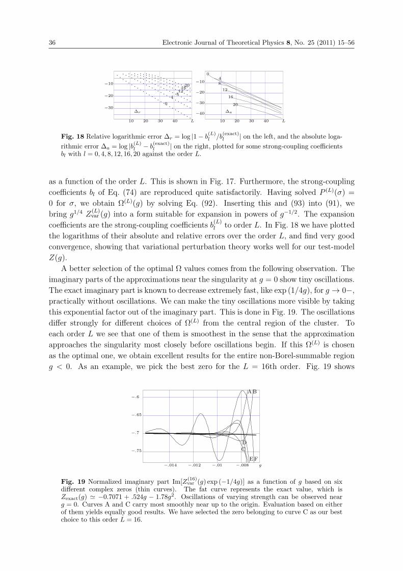
36 Electronic Journal of Theoretical Physics 8, No. 25 (2011) 15–56
L10 20 30 40 L10 20 30 40
−10
−20
−30
−10
−20
−30
−40Δr Δa
0
48121620
04
8
12
16
20
Fig. 18 Relative logarithmic error Δr = log |1− b(L)l /b
(exact)l | on the left, and the absolute loga-
rithmic error Δa = log |b(L)l − b
(exact)l | on the right, plotted for some strong-coupling coefficients
bl with l = 0, 4, 8, 12, 16, 20 against the order L.
as a function of the order L. This is shown in Fig. 17. Furthermore, the strong-coupling
coefficients bl of Eq. (74) are reproduced quite satisfactorily. Having solved P (L)(σ) =
0 for σ, we obtain Ω(L)(g) by solving Eq. (92). Inserting this and (93) into (91), we
bring g1/4 Z(L)var (g) into a form suitable for expansion in powers of g−1/2. The expansion
coefficients are the strong-coupling coefficients b(L)l to order L. In Fig. 18 we have plotted
the logarithms of their absolute and relative errors over the order L, and find very good
convergence, showing that variational perturbation theory works well for our test-model
Z(g).
A better selection of the optimal Ω values comes from the following observation. The
imaginary parts of the approximations near the singularity at g = 0 show tiny oscillations.
The exact imaginary part is known to decrease extremely fast, like exp (1/4g), for g → 0−,practically without oscillations. We can make the tiny oscillations more visible by taking
this exponential factor out of the imaginary part. This is done in Fig. 19. The oscillations
differ strongly for different choices of Ω(L) from the central region of the cluster. To
each order L we see that one of them is smoothest in the sense that the approximation
approaches the singularity most closely before oscillations begin. If this Ω(L) is chosen
as the optimal one, we obtain excellent results for the entire non-Borel-summable region
g < 0. As an example, we pick the best zero for the L = 16th order. Fig. 19 shows
g−.014 −.012 −.01 −.008
−.75
−.7
−.65
−.6AB
CD
EF
Fig. 19 Normalized imaginary part Im[Z(16)var (g) exp (−1/4g)] as a function of g based on six
different complex zeros (thin curves). The fat curve represents the exact value, which isZexact(g) � −0.7071 + .524g − 1.78g2. Oscillations of varying strength can be observed nearg = 0. Curves A and C carry most smoothly near up to the origin. Evaluation based on eitherof them yields equally good results. We have selected the zero belonging to curve C as our bestchoice to this order L = 16.
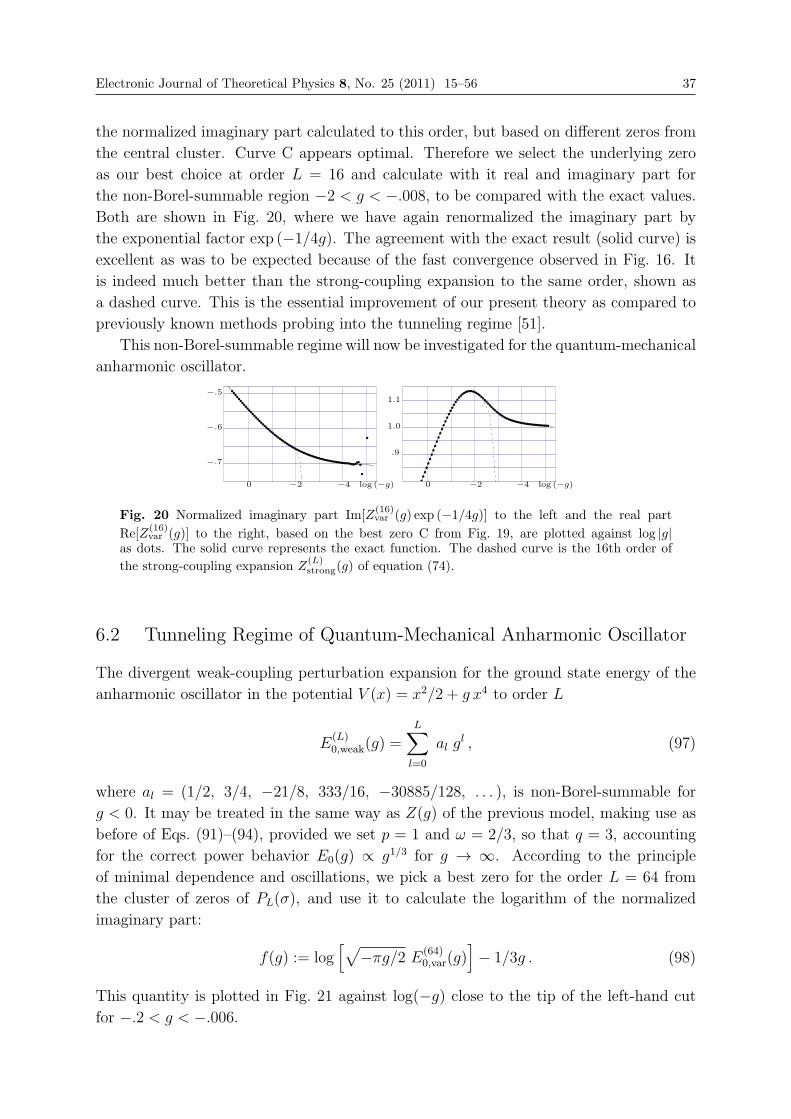
Electronic Journal of Theoretical Physics 8, No. 25 (2011) 15–56 37
the normalized imaginary part calculated to this order, but based on different zeros from
the central cluster. Curve C appears optimal. Therefore we select the underlying zero
as our best choice at order L = 16 and calculate with it real and imaginary part for
the non-Borel-summable region −2 < g < −.008, to be compared with the exact values.Both are shown in Fig. 20, where we have again renormalized the imaginary part by
the exponential factor exp (−1/4g). The agreement with the exact result (solid curve) isexcellent as was to be expected because of the fast convergence observed in Fig. 16. It
is indeed much better than the strong-coupling expansion to the same order, shown as
a dashed curve. This is the essential improvement of our present theory as compared to
previously known methods probing into the tunneling regime [51].
This non-Borel-summable regime will now be investigated for the quantum-mechanical
anharmonic oscillator.
log (−g)0 −2 −4 log (−g)0 −2 −4
.9
1.0
1.1
−.7
−.6
−.5
Fig. 20 Normalized imaginary part Im[Z(16)var (g) exp (−1/4g)] to the left and the real part
Re[Z(16)var (g)] to the right, based on the best zero C from Fig. 19, are plotted against log |g|
as dots. The solid curve represents the exact function. The dashed curve is the 16th order of
the strong-coupling expansion Z(L)strong(g) of equation (74).
6.2 Tunneling Regime of Quantum-Mechanical Anharmonic Oscillator
The divergent weak-coupling perturbation expansion for the ground state energy of the
anharmonic oscillator in the potential V (x) = x2/2 + g x4 to order L
E(L)0,weak(g) =
L∑l=0
al gl , (97)
where al = (1/2, 3/4, −21/8, 333/16, −30885/128, . . . ), is non-Borel-summable forg < 0. It may be treated in the same way as Z(g) of the previous model, making use as
before of Eqs. (91)–(94), provided we set p = 1 and ω = 2/3, so that q = 3, accounting
for the correct power behavior E0(g) ∝ g1/3 for g → ∞. According to the principle
of minimal dependence and oscillations, we pick a best zero for the order L = 64 from
the cluster of zeros of PL(σ), and use it to calculate the logarithm of the normalized
imaginary part:
f(g) := log[√−πg/2 E(64)
0,var(g)]− 1/3g . (98)
This quantity is plotted in Fig. 21 against log(−g) close to the tip of the left-hand cutfor −.2 < g < −.006.

38 Electronic Journal of Theoretical Physics 8, No. 25 (2011) 15–56
−.8
−.4
l(g)
0
−2 −3 −4 −5 log (−g)
Fig. 21 Logarithm of the imaginary part of the ground state energy of the anhar-monic oscillator with the essential singularity factored out for better visualization, l(g) =
log[√−πg/2 E
(64)0,var(g)
]− 1/3g, plotted against small negative values of the coupling constant
−0.2 < g < −.006 where the series is non-Borel-summable. The thin curve represents thedivergent expansion around a critical bubble of Ref. [52]. The fat curve is the 22nd order ap-proximation of the strong-coupling expansion, analytically continued to negative g in the slidingregime calculated in Chapter 17 of the textbook [6].
Comparing our result to older values from semi-classical calculations [52]
f(g) = b1g − b2g2 + b3g
3 − b4g4 + . . . , (99)
with
b1 = 3.95833 b2 = 19.344 b3 = 174.21 b4 = 2177 , (100)
shown in Fig. 21 as a thin curve, we find very good agreement. This expansion contains
the information on the fluctuations around the critical bubble. It is divergent and non-
Borel-summable for g < 0. In Appendix B we have rederived it in a novel way which
allowed us to extend and improve it considerably.
Remarkably, our theory allows us to retrieve the first three terms of this expansion
from the perturbation expansion. Since our result provides us with a regular approxima-
tion to the essential singularity, the fitting procedure depends somewhat on the interval
over which we fit our curve by a power series. A compromise between a sufficiently long
interval and the runaway of the divergent critical-bubble expansion is obtained for a lower
limit g > −.0229 ± .0003 and an upper limit g = −0.006. Fitting a polynomial to thedata, we extract the following first three coefficients:
b1 = 3.9586± .0003 b2 = 19.4± .12 b3 = 135± 18 . (101)
The agreement of these numbers with those in (99) demonstrates that our method is
capable of probing deeply into the critical-bubble region of the coupling constant.
Further evidence for the quality of our theory comes from a comparison with the
analytically continued strong-coupling result plotted to order L = 22 as a fat curve in
Fig. 21. This expansion was derived by a procedure of summing non-Borel-summable
series developed in Chapter 17 of the textbook [6]. It was based on a two-step process:

Electronic Journal of Theoretical Physics 8, No. 25 (2011) 15–56 39
log(−g)−2 −3 −4 −5
−.8
−.6
−.4
−.2
0
8 324 16
Fig. 22 Logarithm of the normalized imaginary part of the ground state energy
log (√−πg/2 E
L)0,var(g))− 1/3g, plotted against log (−g) for orders L = 4, 8, 16, 32 (curves). It
is compared with the corresponding results for L = 64 (points). This is shown for small negativevalues of the coupling constant −0.2 < g < −.006, i.e. in the non-Borel-summable critical-bubbleregion. Fast convergence is easily recognized. Lower orders oscillate more heavily. Increasingorders allow closer approach to the singularity at g = 0−.
the derivation of a strong-coupling expansion of the type (74) from the divergent weak-
coupling expansion, and an analytic continuation of the strong-coupling expansion to
negative g. This method was applicable only for large enough coupling strength where
the strong-coupling expansion converges, the so-called sliding regime. It could not invade
into the tunneling regime at small g governed by critical bubbles, which was treated in [6]
by a separate variational procedure. The present work fills the missing gap by extending
variational perturbation theory to all g arbitrarily close to zero, without the need for a
separate treatment of the tunneling regime.
It is interesting to see, how the correct limit is approached as the order L increases.
This is shown in Fig. 22, based on the optimal zero in each order. For large negative g,
even the small orders give excellent results. Close to the singularity the scaling factor
exp (−1/3g) will always win over the perturbation results. It is surprising, however, howfantastically close to the singularity we can go.
6.3 Dynamic Approach to the Critical-Bubble Regime
Regarding the computational challenges connected with the critical-bubble regime of
small g < 0, it is worth to develop an independent method to calculate imaginary parts
in the tunneling regime. For a quantum-mechanical system with an interaction potential
g V (x), such as a the harmonic oscillator, we may study the effect of an infinitesimal
increase in g upon the system. It induces an infinitesimal unitary transformation of
the Hilbert space. The new Hilbert space can be made the starting point for the next
infinitesimal increase in g. In this way we derive an infinite set of first order ordinary
differential equations for the change of the energy levels and matrix elements (for details
see Appendix C):
E ′n(g) =Vnn(g), (102)
V ′mn(g) =∑k �=n
Vmk(g)Vkn(g)
Em(g)− Ek(g)+∑k �=m
Vmk(g)Vkn(g)
En(g)− Ek(g). (103)

40 Electronic Journal of Theoretical Physics 8, No. 25 (2011) 15–56
g−.3 −.2 −.1
−.2
−.1
Fig. 23 Logarithm of the normalized imaginary part of the ground state energy of the anhar-monic oscillator as solution of the coupled set of differential equations (102), truncated at theenergy level of n = 64 (points), compared with the corresponding quantity from the L = 64thorder of non-Borel-summable variational perturbation theory (curve), both shown as functionsof the coupling constant g.
This system of equations holds for any one-dimensional Schroedinger problem. Individ-
ual differences come from the initial conditions, which are the energy levels En(0) of
the unperturbed system and the matrix elements Vnm(0) of the interaction V (x) in the
unperturbed basis. For a numerical integration of the system a truncation is necessary.
The obvious way is to restrict the Hilbert space to the manifold spanned by the lowest N
eigenvectors of the unperturbed system. For cases like the anharmonic oscillator, which
are even, with even perturbation and with only an even state to be investigated, we may
span the Hilbert space by even basis vectors only. Our initial conditions are thus for
n = 0, 1, 2, . . . , N/2:
E2n(0) =2n+ 1/2 (104)
V2n,2m =0 if m < 0 or m > N/2 (105)
V2n,2n(0) =3(8n2 + 4n+ 1)/4 (106)
V2n,2n±2(0) =(4n+ 3)√(2n+ 1)(2n+ 2)/2 (107)
V2n,2n±4(0) =√(2n+ 1)(2n+ 2)(2n+ 3)(2n+ 4)/4 (108)
(109)
For the anharmonic oscillator with a V (x) = x4 potential, all sums in equation (102) are
finite with at most four terms due to the near-diagonal structure of the perturbation.
In order to find a solution for some g < 0, we first integrate the system from 0 to
|g|, then around a semi-circle g = |g| exp (iϕ) from ϕ = 0 to ϕ = π. The imaginary
part of E0(g) obtained from a calculation with N = 64 is shown in Fig. 23, where it is
compared with the variational result for L = 64. The agreement is excellent. It must
be noted, however, that the necessary truncation of the system of differential equations
introduces an error, which cannot be made arbitrarily small by increasing the truncation
limit N . The approximations are asymptotic sharing this property with the original weak-
coupling series. Its divergence is, however, reduced considerably, which is the reason why
we obtain accurate results for the critical-bubble regime, where the weak-coupling series
fails completely to reproduce the imaginary part.
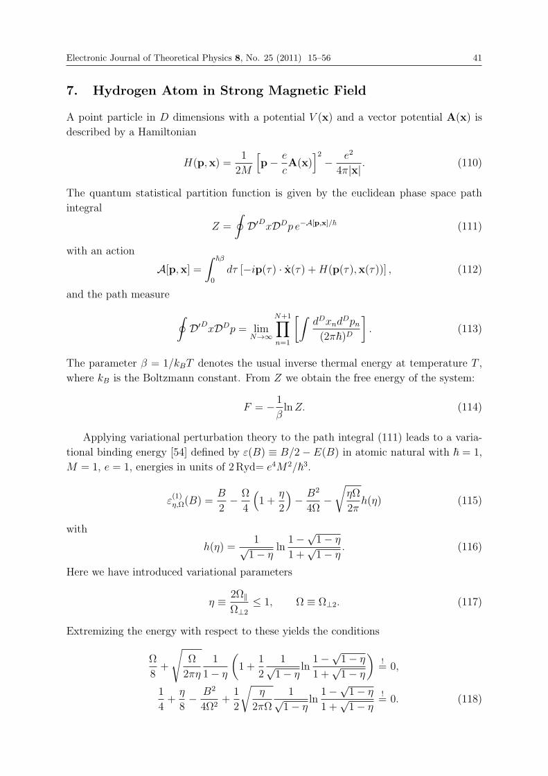
Electronic Journal of Theoretical Physics 8, No. 25 (2011) 15–56 41
7. Hydrogen Atom in Strong Magnetic Field
A point particle in D dimensions with a potential V (x) and a vector potential A(x) is
described by a Hamiltonian
H(p,x) =1
2M
[p− e
cA(x)
]2− e2
4π|x| . (110)
The quantum statistical partition function is given by the euclidean phase space path
integral
Z =
∮D′DxDDp e−A[p,x]/� (111)
with an action
A[p,x] =∫
�β
0
dτ [−ip(τ) · x(τ) +H(p(τ),x(τ))] , (112)
and the path measure ∮D′DxDDp = lim
N→∞
N+1∏n=1
[∫dDxnd
Dpn(2π�)D
]. (113)
The parameter β = 1/kBT denotes the usual inverse thermal energy at temperature T ,
where kB is the Boltzmann constant. From Z we obtain the free energy of the system:
F = − 1βlnZ. (114)
Applying variational perturbation theory to the path integral (111) leads to a varia-
tional binding energy [54] defined by ε(B) ≡ B/2− E(B) in atomic natural with � = 1,
M = 1, e = 1, energies in units of 2Ryd= e4M2/�3.
ε(1)η,Ω(B) =
B
2− Ω
4
(1 +
η
2
)− B2
4Ω−√ηΩ
2πh(η) (115)
with
h(η) =1√1− η
ln1−
√1− η
1 +√1− η
. (116)
Here we have introduced variational parameters
η ≡ 2Ω‖Ω⊥2
≤ 1, Ω ≡ Ω⊥2. (117)
Extremizing the energy with respect to these yields the conditions
Ω
8+
√Ω
2πη
1
1− η
(1 +
1
2
1√1− η
ln1−
√1− η
1 +√1− η
)!= 0,
1
4+η
8− B2
4Ω2+1
2
√η
2πΩ
1√1− η
ln1−
√1− η
1 +√1− η
!= 0. (118)

42 Electronic Journal of Theoretical Physics 8, No. 25 (2011) 15–56
Table 2 Perturbation coefficients up to order B6 for the weak-field expansions of the variationalparameters and the binding energy in comparison to the exact ones of Ref. [55].
n 0 1 2 3
ηn 1.0 − 405π2
7168 ≈ −0.5576 16828965π4
1258815488 ≈ 1.3023 − 3886999332075π6
884272562962432 ≈ −4.2260
Ωn329π ≈ 1.1318 99π
224 ≈ 1.3885 − 1293975π3
19668992 ≈ −2.03982 524431667187π5
27633517592576 ≈ 5.8077
εn − 43π ≈ −0.4244 9π
128 ≈ 0.2209 − 8019π3
1835008 ≈ −0.1355 256449807π5
322256764928 ≈ 0.2435
εn [55] −0.5 0.25 − 53192 ≈ −0.2760 5581
4608 ≈ 1.2112
Expanding the variational parameters into perturbation series of the square magnetic
field B2,
η(B) =∞∑n=0
ηnB2n, Ω(B) =
∞∑n=0
ΩnB2n (119)
and inserting these expansions into the self-consistency conditions (118) and (118) we
obtain order by order the coefficients given in Table 2. Inserting these values into the
expression for the binding energy (115) and expand with respect to B2, we obtain the
perturbation series
ε(1)(B) =B
2−
∞∑n=0
εnB2n. (120)
The first coefficients are also given in Table 2. We find thus the important result that
the first-order variational perturbation solution possesses a perturbative behavior with
respect to the square magnetic field strength B2 in the weak-field limit thus yielding the
correct asymptotic. The coefficients differ in higher order from the exact ones but are
improved by variational perturbation theory [6].
In a strong magnetic field one has
Ω⊥ � 2Ω‖, Ω‖ � B (121)
and the variational expression simplifies to
ε(1)Ω⊥,Ω‖ =
B
2−(Ω⊥4+
B2
4Ω⊥+Ω‖4+
√Ω‖πln
Ω‖2Ω⊥
), (122)
which is minimal at √Ω‖ = −
2√π
(lnΩ‖ − lnΩ⊥ + 2− ln 2
), (123)
Ω⊥ = 2
√Ω‖π+B
√1 + 4
Ω‖πB2
. (124)
Expanding the second conditions as
Ω⊥ = B + 2
√Ω‖π+ 2
Ω‖πB
− 4Ω2‖
π2B3+ . . . , (125)

Electronic Journal of Theoretical Physics 8, No. 25 (2011) 15–56 43
and inserting only the first two terms into the first condition (123), we neglect terms of
order 1/B, and find √Ω‖ ≈
2√π
(lnB − lnΩ
(1)‖ + ln 2− 2
). (126)
To obtain a tractable approximation for Ω‖, we perform some iterations starting from√Ω
(1)‖ =
2√πln 2Be−2 (127)
Reinserting this on the right-hand side of Eq. (126), one obtains the second iteration√Ω
(2)‖ . We stop this procedure after an additional reinsertion which yields√Ω
(3)‖ =
2√π
(ln 2Be−2 − 2ln
[2√π
{ln 2Be−2 − 2ln
(2√πln 2Be−2
)}]). (128)
The reader may convince himself that this iteration procedure indeed converges. For a
subsequent systematical extraction of terms essentially contributing to the binding energy,
the expression (128) is not satisfactory. Therefore it is better to separate the leading term
in the curly brackets and expand the logarithm of the remainder. Then this procedure
is applied to the expression in the square brackets and so on. Neglecting terms of order
ln−3B, we obtain √Ω
(3)‖ ≈ 2√
π
(ln 2Be−2 + ln
π
4− 2lnln 2Be−2
). (129)
The double-logarithmic term can be expanded in a similar way as described above:
lnln 2Be−2 = ln
[lnB
(1 +
ln 2− 2
lnB
)]= lnlnB +
ln 2− 2
lnB− 1
2
(ln 2− 2)2
ln2B+O(ln−3B).
(130)
Thus the expression (129) may be rewritten as√Ω
(3)‖ =
2√π
(lnB − 2lnlnB +
2a
lnB+
a2
ln2B+ b
)+O(ln−3B) (131)
with abbreviations
a = 2− ln 2 ≈ 1.307, b = lnπ
2− 2 ≈ −1.548. (132)
The first observation is that the variational parameter Ω‖ is always much smaller than
Ω⊥ in the high B-field limit. Thus we can further simplify the approximation (125) by
replacing
Ω⊥ ≈ B
(1 +
2
B
√Ω‖π
)−→ B (133)
without affecting the following expression for the binding energy. Inserting the solu-
tions (131) and (133) into the equation for the binding energy (122) and expanding the
logarithmic term once more as described, we find up to the order ln−2B:
ε(1)(B) =1
π(ln2B − 4 lnB lnlnB + 4 ln2lnB − 4b lnlnB + 2(b+ 2) lnB + b2
− 1
lnB[8 ln2lnB − 8b lnlnB + 2b2]) +O(ln−2B) (134)

44 Electronic Journal of Theoretical Physics 8, No. 25 (2011) 15–56
Table 3 Example for the competing leading six terms in Eq. (134) at B = 105B0 ≈ 2.35×10¹⁴ G.
(1/π)ln2B −(4/π)lnB lnlnB (4/π) ln2lnB −(4b/π) lnlnB [2(b + 2)/π] lnB b2/π
42.1912 −35.8181 7.6019 4.8173 3.3098 0.7632
Note that the prefactor 1/π of the leading ln2B-term differs from a value 1/2 obtained
by Landau and Lifschitz [56]. Our different value is a consequence of using a harmonic
trial system. The calculation of higher orders in variational perturbation theory would
improve the value of the prefactor.
At a magnetic field strength B = 105B0, which corresponds to 2.35× 10¹⁰T = 2.35×10¹⁴G, the contribution from the first six terms is 22.87 [2Ryd]. The next three terms
suppressed by a factor ln−1B contribute −2.29 [2Ryd], while an estimate for the ln−2B-terms yields nearly −0.3 [2Ryd]. Thus we find
ε(1)(105) = 20.58± 0.3 [2Ryd]. (135)
This is in very good agreement with the value 20.60 [2Ryd] obtained from an accurate
numerical treatment [58].
Table 3 lists the values of the first six terms of Eq. (134). This shows in particular
the significance of the second-leading term −(4/π)lnB lnlnB, which is of the same order
of the leading term (1/π)ln2B but with an opposite sign. In Fig. 24, we have plotted the
expression
εL(B) =1
2ln2B (136)
from Landau and Lifschitz [56] to illustrate that it gives far too large binding energies
even at very large magnetic fields, e.g. at 2000B0 ∝ 1012G.
This strength of magnetic field appears on surfaces of neutron stars (1010−1012G). Arecently discovered new type of neutron star is the so-called magnetar. In these, charged
particles such as protons and electrons produced by decaying neutrons give rise to the
giant magnetic field of 1015G. Magnetic fields of white dwarfs reach only up to 106−108G.All these magnetic field strengths are far from realization in experiments. The strongest
magnetic fields ever produced in a laboratory were only of the order 105G, an order of
magnitude larger than the fields in sun spots which reach about 0.4× 10⁴G. Recall, for
comparison, that the earth’s magnetic field has the small value of 0.6G.
The nonleading terms in Eq. (134) give important contributions to the asymptotic
behavior even at such large magnetic fields, as we can see in Fig. 24. It is an unusual
property of the asymptotic behavior that the absolute value of the difference between the
Landau-expression (136) and our approximation (134) diverges with increasing magnetic
field strengths B, only the relative difference decreases.
8. Appendix A: Modification of Principle of Minimal Sensitivity
The naive quantum mechanical variational perturbation theory has been used by many
authors under the name δ-expansion. This name stems from the fact that one may write
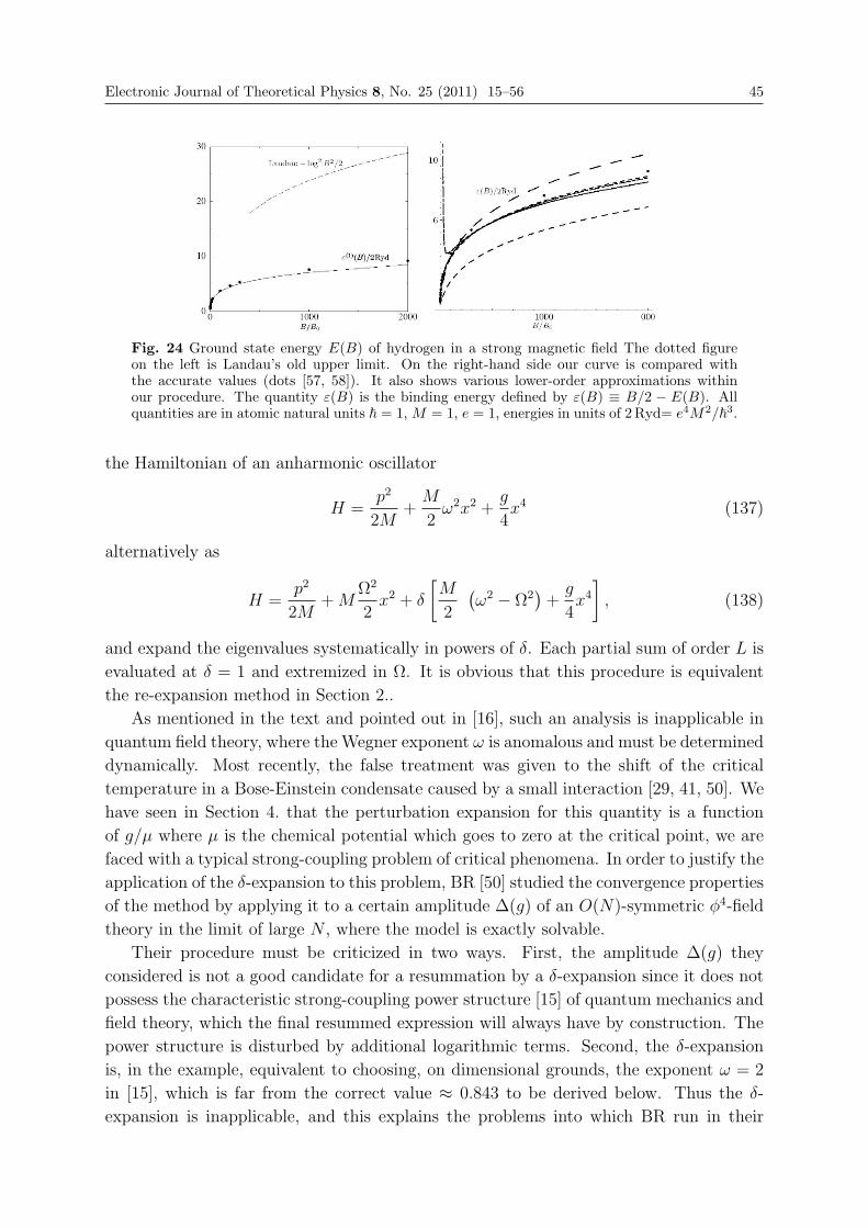
Electronic Journal of Theoretical Physics 8, No. 25 (2011) 15–56 45
Fig. 24 Ground state energy E(B) of hydrogen in a strong magnetic field The dotted figureon the left is Landau’s old upper limit. On the right-hand side our curve is compared withthe accurate values (dots [57, 58]). It also shows various lower-order approximations withinour procedure. The quantity ε(B) is the binding energy defined by ε(B) ≡ B/2 − E(B). Allquantities are in atomic natural units � = 1, M = 1, e = 1, energies in units of 2 Ryd= e4M2/�3.
the Hamiltonian of an anharmonic oscillator
H =p2
2M+M
2ω2x2 +
g
4x4 (137)
alternatively as
H =p2
2M+M
Ω2
2x2 + δ
[M
2
(ω2 − Ω2
)+g
4x4], (138)
and expand the eigenvalues systematically in powers of δ. Each partial sum of order L is
evaluated at δ = 1 and extremized in Ω. It is obvious that this procedure is equivalent
the re-expansion method in Section 2..
As mentioned in the text and pointed out in [16], such an analysis is inapplicable in
quantum field theory, where the Wegner exponent ω is anomalous and must be determined
dynamically. Most recently, the false treatment was given to the shift of the critical
temperature in a Bose-Einstein condensate caused by a small interaction [29, 41, 50]. We
have seen in Section 4. that the perturbation expansion for this quantity is a function
of g/μ where μ is the chemical potential which goes to zero at the critical point, we are
faced with a typical strong-coupling problem of critical phenomena. In order to justify the
application of the δ-expansion to this problem, BR [50] studied the convergence properties
of the method by applying it to a certain amplitude Δ(g) of an O(N)-symmetric φ4-field
theory in the limit of large N , where the model is exactly solvable.
Their procedure must be criticized in two ways. First, the amplitude Δ(g) they
considered is not a good candidate for a resummation by a δ-expansion since it does not
possess the characteristic strong-coupling power structure [15] of quantum mechanics and
field theory, which the final resummed expression will always have by construction. The
power structure is disturbed by additional logarithmic terms. Second, the δ-expansion
is, in the example, equivalent to choosing, on dimensional grounds, the exponent ω = 2
in [15], which is far from the correct value ≈ 0.843 to be derived below. Thus the δ-
expansion is inapplicable, and this explains the problems into which BR run in their

46 Electronic Journal of Theoretical Physics 8, No. 25 (2011) 15–56
resummation attempt. Most importantly, they do not find a well-shaped plateau of
the variational expressions Δ(L)(g, z) as a function of z which would be necessary for
invoking the principle of minimal sensitivity. Instead, they observe that the zeros of the
first derivatives ∂zΔ(L)(g, z) run away far into the complex plain. Choosing the complex
solutions to determine their final resummed value misses the correct one by 3% up to the
35th order.
One may improve the situation by trying out various different ω-values and choosing
the best of them yielding an acceptable plateau in Δ(g, z). This happens for ω ≈ 0.843.
However, even for this optimal value, the resummation result never converges to the
correct limit. For Δ(g) the error happens to be numerically small, only 0.1%, but it will
be uncontrolled in physical problems where the result is unknown.
Let us explain these points in more detail. BR consider the weak-coupling series with
the reexpansion parameter δ:
Δ(δ, g) = −∞∑l=1
(− δ g√
1− δ
)l
al , where al ≡∫ ∞
0
K(x)f l(x) dx , (139)
with
K(x) ≡ 4x2
π(1 + x2)2, f(x) ≡ 2
xarctan
x
2. (140)
The geometric series in (139) can be summed exactly, and the result may formally be
reexpanded into a strong-coupling series in h ≡√1− δ/(δ g):
Δ(δ, g) =
∫ ∞
0
K(x)δgf(x)√
1− δ + δgf(x)dx =
∞∑m=0
bm (−h)m ,where bm =
∫ ∞
0
K(x)f−m(x)dx.
(141)
The strong-coupling limit is found for h → 0 where Δ → b0 =∫∞0dxK(x) = 1. The
approach to this limit is, however, not given by a strong-coupling expansion of the form
(141). This would only happen if all the integrals bm were to exist which, unfortunately,
is not the case since all integrals for bm with m > 0 diverge at the upper limit, where
f(x) =2
xarctan
x
2∼ π
x. (142)
The exact behavior of Δ in the strong-coupling limit h → 0 is found by studying the
effect of the asymptotic π/x-contribution of f(x) to the integral in (141). For f(x) = π/x
we obtain ∫ ∞
0
K(x)1
1 + h/f(x)dx =
π4 + 2πh− πh+ 2h+ 4πh log h/π
(π + h). (143)
The logarithm of h shows a mismatch with the general asymptotic form of the result [15],
which and prevents the expansion (139) to be a candidate for variational perturbation
theory.

Electronic Journal of Theoretical Physics 8, No. 25 (2011) 15–56 47
We now explain the second criticism. Suppose we ignore the just-demonstrated fun-
damental obstacle and follow the rules of the δ-expansion, defining the Lth order ap-
proximant Δ(δ,∞) by expanding (139) in powers of δ up to order δL, setting δ = 1, and
defining z ≡ g. Then we obtain the Lth variational expression for b0:
b(L)0 (ω, z) =
L∑l=1
alzl
(L− l + l/ω
L− l
), (144)
with ω = 2, to be optimized in z. This ω-value would only be adequate if the approach
to the strong-coupling limit behaved like A+B/h2 + . . . , rather than (143). This is the
reason why BR find no real regime of minimal sensitivity on z.
0.5 1 1.5 2.5-0.5
0
0.5
1
Fig. 25 Plot of 1 − b(L)0 (ω, z) versus z for L = 10 and ω = 0.6, 0.843, 1, 2 . The curve
with ω = 0.6 shows oscillations. They decrease with increasing ω and becomes flat at aboutω = 0.843. Further increase of ω tilts the plateau and shows no regime of minimal sensitivity.At the same time, the minimum of the curve rises rapidly above the correct value of 1− b0 = 0,as can be seen from the upper two curves for ω = 1 and ω = 2, respectively.
Let us attempt to improve the situation by determining ω dynamically by making the
plateau in the plots of Δ(L)(ω, h) versus h horizontal for several different ω-values. The
result is ω ≈ 0.843, quite far from the naive value 2. This value can also be estimated
by inspecting plots of Δ(L)(ω, h) versus h for several different ω-values in Fig. 25, and
selecting the one producing minimal sensitivity.
It produces reasonable results also in higher orders, as is seen in Fig. 26. The
approximations appear to converge rapidly. But the limit does not coincide with the
known exact value, although it happens to lie numerically quite close. Extrapolating the
successive approximations by an extremely accurate fit to the analytically known large-
order behavior [15] with a function b(L)0,plateau(ω = 0.843) = A+B L−κ, we find convergence
to A = 1 − 0.001136, which misses the correct limit A = 1. The other two parameters
are fitted best by B = −0.002495 and κ = 0.922347 (see Fig. 27).
We may easily convince ourselves by numerical analysis that the error in the limiting
value is indeed linked to the failure of the strong-coupling behavior (143) to have the power
structure of [15]. For this purpose we change the function f(x) in equation (140) slightly
into f(x)→ f(x) = f(x) + 1, which makes the integrals for bm in (141) convergent. The
exact limiting value 1 of Δ remaines unchanged, but b(L)0 acquires now the correct strong-
coupling power structure of [15]. For this reason, we can easily verify that the application
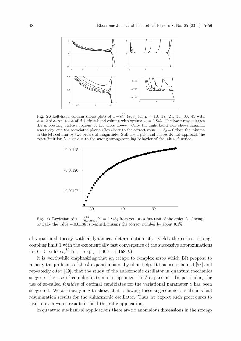
48 Electronic Journal of Theoretical Physics 8, No. 25 (2011) 15–56
0.5 1 1.50
0.2
0.4
0 1 2
-0.0015
-0.0012
-0.0009
0 0.5 1 1.5
-1
0
1
0 1 2
-1
0
1
Fig. 26 Left-hand column shows plots of 1 − b(L)0 (ω, z) for L = 10, 17, 24, 31, 38, 45 with
ω = 2 of δ-expansion of BR, right-hand column with optimal ω = 0.843. The lower row enlargesthe interesting plateau regions of the plots above. Only the right-hand side shows minimalsensitivity, and the associated plateau lies closer to the correct value 1− b0 = 0 than the minimain the left column by two orders of magnitude. Still the right-hand curves do not approach theexact limit for L→∞ due to the wrong strong-coupling behavior of the initial function.
20 40 60
-0.00125
-0.00126
-0.00127
Fig. 27 Deviation of 1 − b(L)0,plateau(ω = 0.843) from zero as a function of the order L. Asymp-
totically the value −.001136 is reached, missing the correct number by about 0.1%.
of variational theory with a dynamical determination of ω yields the correct strong-
coupling limit 1 with the exponentially fast convergence of the successive approximations
for L→∞ like b(L)0 ≈ 1− exp (−1.909− 1.168 L).
It is worthwhile emphasizing that an escape to complex zeros which BR propose to
remedy the problems of the δ-expansion is really of no help. It has been claimed [53] and
repeatedly cited [49], that the study of the anharmonic oscillator in quantum mechanics
suggests the use of complex extrema to optimize the δ-expansion. In particular, the
use of so-called families of optimal candidates for the variational parameter z has been
suggested. We are now going to show, that following these suggestions one obtains bad
resummation results for the anharmonic oscillator. Thus we expect such procedures to
lead to even worse results in field-theoretic applications.
In quantum mechanical applications there are no anomalous dimensions in the strong-

Electronic Journal of Theoretical Physics 8, No. 25 (2011) 15–56 49
coupling behavior of the energy eigenvalues. The growth parameters α and ω can be
directly read off from the Schrodinger equation; they are α = 1/3 and ω = 2/3 for the
anharmonic oscillator (see Appendix A). The variational perturbation theory is applicable
for all couplings strengths g as long as b(L)0 (z) becomes stationary for a certain value of
z. For higher orders L it must exhibit a well-developed plateau. Within the range of the
plateau, various derivatives of b(L)0 (z) with respect to z will vanish. In addition there will
be complex zeros with small imaginary parts clustering around the plateau. They are,
however, of limited use for designing an automatized computer program for localizing the
position of the plateau. The study of several examples shows that plotting b(L)0 (z) for
various values of α and ω and judging visually the plateau is by far the safest method,
showing immediately which values of α and ω lead to a well-shaped plateau.
Let us review briefly the properties of the results obtained from real and complex
zeros of ∂zb(L)0 (z) for the anharmonic oscillator. In Fig. 28, the logarithmic error of b
(L)0
is plotted versus the order L. At each order, all zeros of the first derivative are exploited.
To test the rule suggested in [53], only the real parts of the complex roots have been used
to evaluate b(L)0 . The fat points represent the results of real zeros, the thin points stem
from the real parts of complex zeros. It is readily seen that the real zeros give the better
result. Only by chance may a complex zero yield a smaller error. Unfortunately, there is
no rule to detect these accidental events. Most complex zeros produce large errors.
0 20 40 60 80-40
-30
-20
-10
0
Fig. 28 Logarithmic error of the leading strong-coupling coefficient b(L)0 of the ground state
energy of the anharmonic oscillator with x4 potential. The errors are plotted over the order Lof the variational perturbation expansion. At each order, all zeros of the first derivative have
been exploited. Only the real parts of the complex roots have been used to evaluate b(L)0 . The
fat points show results from real zeros, the smaller points those from complex zeros, size isdecreasing with distance from real axis.
We observe the existence of families described in detail in the textbook [6] and redis-
covered in Ref. [53]. These families start at about N = 6, 15, 30, 53, respectively. But
each family fails to converge to the correct result. Only a sequence of selected members in
each family leads to an exponential convergence. Consecutive families alternate around
the correct result, as can be seen more clearly in a plot of the deviations of b(L)0 from their
L → ∞ -limit in Fig. 29, where values derived from the zeros of the second derivative
of b(L)0 have been included.These give rise to accompanying families of similar behavior,

50 Electronic Journal of Theoretical Physics 8, No. 25 (2011) 15–56
0 20 40 60 80
-1 ·10-10
-5 ·10-11
0
5·10-11
0 20 40 60 80
-1 ·10-13
0
1·10-13
2·10-13
0 20 40 60 80
-0.00003
-0.00002
-0.00001
0
0.00001
0.00002
0 20 40 60 80
0
1·10-8
2·10-8
3·10-8
4·10-8
5·10-8
Fig. 29 Deviation of the coefficient b(L)0 from the exact value is shown as a function of pertur-
bative order L on a linear scale. As before, fat dots represent real zeros. In addition to Fig. 28,
the results obtained from zeros of the second derivative of b(L)0 are shown. They give rise to own
families with smaller errors by about 30%. At N = 6, the upper left plot shows the start of two
families belonging to the first and second derivative of b(L)0 , respectively. The deviations of both
families are negative. On the upper right-hand figure, an enlargement visualizes the next twofamilies starting at N = 15. Their deviations are positive. The bottom row shows two moreenlargements of families starting at N = 30 and N = 53, respectively. The deviations alternateagain in sign.
deviating with the same sign pattern from the exact result, but lying closer to the correct
result by about 30.
9. Appendix B: Ground-State Energy from Imaginary Part
We determine the ground state energy function E0(g) for the anharmonic oscillator on
the cut, i.e. for g < 0 in the bubble region, from the weak coupling coefficients al of
equation (97). The behavior of the al for large l can be cast into the form
al/al−1 = −L∑
j=−1βj l
−j . (145)
The βj can be determined by a high precision fit to the data in the large l region of250 < l < 300 to be
β−1, 0, 1, ... =
{3, −3
2,
95
24,
113
6,
391691
3456,
40783
48,
1915121357
248832,
10158832895
124416,
70884236139235
71663616,
60128283463321
4478976,
286443690892
1423,
144343264152266
43743,
351954117229
6,
2627843837757582
2339,
230619387597863
10,
12122186977970425
24,
41831507430222441029
3550, . . .
}, (146)

Electronic Journal of Theoretical Physics 8, No. 25 (2011) 15–56 51
where the rational numbers up to j = 6 are found to be exact, whereas the higher ones are approxima-
tions.
Equation (145) can be read as recurrence relation for the coefficients al. Now we construct an ordinary
differential equation for E(g) := E(L)0,weak(g) from this recurrence relation and find:⎡⎣(g d
dg
)L
+ g
L+1∑j=0
βL−j
(gd
dg+ 1
)j⎤⎦E(g) = 0 . (147)
All coefficients being real, real and imaginary part of E(g) each have to satisfy this equation separately.
The point g = 0, however, is not a regular point. We are looking for a solution, which is finite when
approaching it along the negative real axis. Asymptotically E(g) has to satisfy E(g) � exp (1/gβ−1) =
exp (1/3g). Therefore we solve (147) with the ansatz
E(g) = gα exp
(1
3g−∑k=1
bk(−g)k)
(148)
to obtain α = −1/2 and
b1,2,3,... =
{95
24,
619
32,
200689
1152,
2229541
1024,
104587909
3072,
7776055955
12288,
9339313153349
688128,
172713593813181
524288,
1248602386820060039
139886592,
14531808399402704160316631
54391637278720,
12579836720279641736960567921
1435939224158208,
109051824717547897884794645746723
348951880031797248,
45574017678173074497482074500364087
3780312033677803520. . . . (149)
This is in agreement with equation (100) and an improvement compared to the WKB results of [52].
Again, the first six rational numbers are exact, followed by approximate ones.
10. Appendix C: First-Order Differential Equations for En(g)
Given a one-dimensional quantum system
(H0 + g V )|n, g〉 = En(g)|n, g〉 (150)
with Hamiltonian H = H0 + g V , eigenvalues En(g) and eigenstates |n, g〉 we consider an infinitesimal
increase dg in the coupling constant g. The eigenvectors will undergo a small change:
|n, g + dg〉 = |n, g〉+ dg∑k �=n
unk|k, g〉 (151)
so that
d
dg|n, g〉 =
∑k �=n
unk|k, g〉 . (152)
Given this, we take the derivative of (150) with respect to g and multiply by 〈m, g| from the left to
obtain:
〈m, g|V − E′n(g)|n, g〉 =
∑k �=n
unk〈m, g|H0 + g V − En(g)|k, g〉 . (153)
Setting now m = n and m �= n in turn, we find:
E′n(g) =Vnn(g) (154)
Vmn(g) =unm (Em(g)− En(g)) , (155)

52 Electronic Journal of Theoretical Physics 8, No. 25 (2011) 15–56
where Vmn(g) = 〈m, g|V |n, g〉.Equation (154) governs the behavior of the eigenvalues as functions of the coupling constant g. In order
to have a complete system of differential equations, we must also determine how the Vmn(g) change,
when g changes. With the help of equations (152) and (155), we obtain:
V ′mn =
∑k �=m
u∗mk〈k, g|V |n, g〉+
∑k �=n
unk〈m, g|V |k, g〉 (156)
V ′mn =
∑k �=m
VmkVkn
Em − Ek+∑k �=n
VmkVkn
En − Ek. (157)
Equations (154) and (157) together describe a complete set of differential equations for the energy eigen-
values En(g) and the matrix-elements Vnm(g). The latter determine via (155) the expansion coefficients
umn(g). Initial conditions are given by the eigenvalues En(0) and the matrix elements Vnm(0) of the
unperturbed system.
References
[1] J. Goldstone, A. Salam, and S. Weinberg, Phys. Rev. 127 , 965 (1962).
[2] C. De Dominicis. J. Math. Phys. 3, 983 (1962).
[3] R.P. Feynman, Statistical Mechanics, Benjamin, Reading, 1972.
[4] R.P. Feynman and H. Kleinert, Phys. Rev. A 34, 1986(http//physik.fu-berlin.de/~kleinert/159/159.pdf).
[5] H. Kleinert Phys. Lett. A 173, 332 (1993)(http://physik.fu-berlin.de/~kleinert/213).
[6] H. Kleinert, Path Integrals in Quantum Mechanics, Statistics, Polymer Physics, andFinancial Markets, World Scientific, Singapore, 2009(http://www.physik.fu-berlin.de/~kleinert/b5).
[7] H. Kleinert, Annals of Physics 266, 135 (1998)(http://physik.fu-berlin.de/~kleinert/255/255.pdf).
[8] J.A. Lipa, D.R. Swanson, J.A. Nissen, T.C.P. Chui and U.E. Israelsson, Phys. Rev.Lett. —bf 76, 944 (1996); J.A. Lipa, D. R. Swanson, J.A. Nissen, Z.K. Geng, P.R.Williamson, D.A. Stricker, T.C.P. Chui, U.E. Israelsson and M. Larson, Phys. Rev.Lett. —bf 84, 4894 (2000).
[9] H. Kleinert, Phys. Rev. D 60, 085001 (1999) (hep-th/9812197); Phys.Lett. A 277,205 (2000) (cond-mat/9906107).
[10] V.I. Yukalov, Theor. Math. Phys. 28, 652-660 (1976); Physica A 89, 363-372(1977); Ann. Physik 36, 31 (1979); 37, 171 (1980); 38, 419 (1981); P.M. Stevenson,Phys. Rev. D 30, 1712 (1985); D 32, 1389 (1985); P.M. Stevenson and R. Tarrach,Phys. Lett. B 176, 436 (1986).
[11] W. Janke, H. Kleinert, Phys. Rev. Lett. 75, 2787 (1995) (quant-ph/9502019).
[12] E.J. Weniger, Phys. Rev. Lett. 77, 2859 (1996); see also F. Vinette and J. Cızek,J. Math. Phys. 32, 3392 (1991).
[13] H Kleinert and W. Janke, Phys. Lett. A 206, 283 (1995) (quant-ph/9509005).
[14] R. Guida, K. Konishi, H. Suzuki, Ann. Phys. (N.Y.) 249, 109 (1996).

Electronic Journal of Theoretical Physics 8, No. 25 (2011) 15–56 53
[15] H. Kleinert, Phys. Rev. D 57, 2264 (1998) (cond-mat/9801167); Phys. Rev. D 58,107702 (1998) (cond-mat/9803268).
[16] B. Hamprecht and H. Kleinert, Phys. Rev. D 68, 065001 (2003) (hep-th/0302116).
[17] R. Seznec and J. Zinn-Justin, J. Math. Phys. 20, 1398 (1979). This paper hasdeveloped important techniques for understanding the convergence mechanism ofvariational perturbation theory.
[18] H. Kleinert and V. Schulte-Frohlinde, Critical Phenomena in Φ4-Theory, WorldScientific, Singapore, 2001 (http://www.physik.fu-berlin.de/~kleinert/b8).
[19] J. Zinn-Justin, Quantum Field Theory and Critical Phenomena, Clarendon, Oxford,1989.
[20] See Section 19.4 in [18].
[21] F.J. Wegner, Phys. Rev. B 5, 4529 (1972); B 6, 1891 (1972).
[22] B.G. Nickel, D.I. Meiron, and G.B. Baker, Univ. of Guelph preprint 1977(unpublished). The preprint is readable on the WWW athttp://www.physik.fu-berlin.de/~kleinert/nickel/guelph.pdf;The results are cited and used in Chapters 19 and 20. They were axtended to sevenloops byD.B. Murray and B.G. Nickel, Univ. of Guelph preprint 1991.The additional g7 coefficients of the renormalization group functions are listed inSection 20.4 of the textbook [18].
[23] See Section 20.2 in [18].
[24] H. Kleinert, Phys. Rev. D 60, 085001 (1999) (hep-th/9812197), see Fig. 9; Phys.Lett.A 277, 205 (2000) (cond-mat/9906107).
[25] M. Holzmann, G. Baym, J.-P. Blaizot and F. Laloe, Phys. Rev. Lett. 87, 120403(2001).
[26] P. Arnold, G. Moore and B. Tomasik, cond-mat/0107124.
[27] J. Zinn-Justin, Quantum Field Theory and Critical Phenomena (Oxford UniversityPress, Oxford, England, 1996).
[28] M. Bijlsma and H. T. C. Stoof, Phys. Rev. A 54, 5085 (1996)
[29] F.F. de Souza Cruz, M.B. Pinto and R.O. Ramos, Phys. Rev. A 65, 053613 (2002)(cond-mat/0112306).
[30] E. Braaten, and E. Radescu, Phys. Rev. A 66, 063601 (2002) (cond-mat/0206186).
[31] These are the results of [30]. They differ from those of Refs. [29] which are a3 =0.644519, a41 = 0.87339, a42 = 3.15905, a43 = 1.70959, a44 = 4.4411, a45 = 2.37741. Thecoefficients of the series (57) to be resummed differ mainly in the last term: f−1 =−126.651 10−4, f0 = 0, f1= −4.04857 10−4, f2= 2.40587 10−4, f3= −2.06849 10−4.
[32] H. Kleinert, Strong-Coupling Behavior of Phi4-Theories and Critical Exponents,Phys. Rev. D 57 , 2264 (1998); Addendum: Phys. Rev. D 58 , 107702 (1998) (cond-mat/9803268); Seven Loop Critical Exponents from Strong-Coupling φ4-Theory inThree Dimensions , Phys. Rev. D 60 , 085001 (1999) (hep-th/9812197); Theory andSatellite Experiment on Critical Exponent alpha of Specific Heat in Superfluid HeliumPhys. Lett. A 277, 205 (2000) (cond-mat/9906107).

54 Electronic Journal of Theoretical Physics 8, No. 25 (2011) 15–56
[33] H. Kleinert, Strong-Coupling φ4-Theory in 4− ε Dimensions, and Critical Exponent ,Phys. Lett. B 434 , 74 (1998) (cond-mat/9801167); Critical Exponents without beta-Function, Phys. Lett. B 463, 69 (1999) (cond-mat/9906359).
[34] See [29, 30, 41] and references cited there.
[35] With standard normalization conditions used in the 3-dimensional φ4-theory, theapproach to scaling is governed by Wegner’s exponent ω (see [32]). The presentdefinition of m differs from the inverse correlation length m = ξ−1 by a factor:m = mZ−1φ ∝ mm−η/2 for m → 0. This changes the exponent of approach toω′ = ω/(1− η/2). I thank B. Kastening for noting this.
[36] P. Arnold and G. Moore, Phys. Rev. Lett. 87, 120401 (2001); Phys. Rev. E 64,066113 (2001). The authors derive a 1/N correction factor (1 − 0.527/N) to theleading N →∞ result.
[37] V.A. Kashurnikov, N.V. Prokof’ev and B.V. Svistunov, Phys. Rev. Lett. 87, 120402(2001).
[38] G. Baym, J.-P. Blaizot M. Holzmann, F. Laloe and D. Vautherin, Phys. Rev. Lett.83, 1703 (1999).
[39] G. Baym, J.-P. Blaizot and J. Zinn-Justin, Europhys. Lett. 49, 150 (2000).
[40] P. Arnold and B. Tomasik, Phys. Rev. A62, 063604 (2000).This paper starts out from the 3+1-dimensional initial theory and derives from it thethree-dimensional effective classical field theory, the field-theoretic generalization ofthe quantum-mechanical effective classical potential ofR.P Feynman and H. Kleinert, Phys. Rev. A 34, 5080 (1986). This reduction programwas started for the Bose-Einstein gas byA.M.J. Schakel, Int. J. Mod. Phys. B 8, 2021 (1994); J. Mod. Phys. B 8, 2021(1994); Boulevard of Broken Symmetries , Habilitationsschrift, FU-Berlin, (cond-mat/9805152) (1998).Unfortunately, Schakel did not go beyond the one-loop level so that he was happyto have found a positive shift ΔTc/Tc, and did see the cancellation at the two-looplevel. See his recent paper in J. Phys. Stud. 7, 140 (2003) (cond-mat/0301050).
[41] F.F. de Souza Cruz, M.B. Pinto and R.O. Ramos, Phys. Rev. B 64, 014515 (2001).
[42] P. Grueter, D. Ceperley, F. Laloe, Phys. Rev. Lett. 79, 3549 (1997) (cond-mat/9707028).
[43] See Eq. (20.23) in the textbook [18] or S.E. Derkachov, J.A. Gracey, and A.N.Manashov, Eur. Phys. J. C 2, 569 (1998) (hep-ph/9705268).
[44] W. Janke and H. Kleinert, Phys. Lett. A 117, 353 (1986)(http://www.physik.fu-berlin.de/~kleinert/133); Phys. Rev. Lett. 58, 144(1986). H. Kleinert, Phys. Lett. A 257, 269 (1999) (cond-mat/9811308); M.Bachmann, H. Kleinert, A. Pelster, Phys. Lett. A 261, 127 (1999) (cond-mat/9905397); Physical Review E 63, 051709/1-10 (2001) (cond-mat/0011281); seealso B. Kastening, Phys.Rev. A 68, 061601 (2003) (cond-mat/0303486); Phys.Rev.A 69, 043613 (2004) (cond-mat/0309060); Phys. Rev. E 73, 011101 (2006) (cond-mat/0508614); Phys. Rev. A 70, 043621 (2004) (cond-mat/0406035).
[45] J.S. Langer, Ann. Phys. 41, 108 (1967).
[46] C.M. Bender and T.T. Wu, Phys. Rev. 184, 1231 (1969);
[47] S. Coleman, Nucl. Phys. B 298, 178 (1988).

Electronic Journal of Theoretical Physics 8, No. 25 (2011) 15–56 55
[48] B.Bellet, P.Garcia, A.Neveu, Int. J. of Mod. Phys. A 11, 5587(1997)
[49] J.-L. Kneur, D. Reynaud, (hep-th/0205133v2). See also [50], [29], [41].
[50] E. Braaten, E. Radescu, (cond-math/0206186v1).
[51] The low-order results were first obtained byH. Kleinert, Phys. Lett. B 300, 261 (1993)(http://www.physik.fu-berlin.de/~kleinert/214),and extended by R. Karrlein and H. Kleinert, Phys. Lett. A 187, 133 (1994) (hep-th/9504048).
[52] J. Zinn-Justin, J. Math Phys. 22(3), 511 (1981). The first 10 coefficients of expansion(99) are calculated.
[53] B.Bellet, P.Garcia, A.Neveu, Int. J. of Mod. Phys. A11, 5587(1997). The familystructure of optimal variational parameters emphasized in this paper was discussedin great detail earlier in Chapter 5 of the textbook [6], but with correct applicationrules.
[54] M. Bachmann, H. Kleinert, and A. Pelster, Phys. Rev. A 62, 52509 (2000) (quant-ph/0005074), Phys. Lett. A 279, 23 (2001) (quant-ph/000510).
[55] J.E. Avron, B.G. Adams, J. Cızek, M. Clay, M.L. Glasser, P. Otto, J. Paldus, andE. Vrscay, Phys. Rev. Lett. 43, 691 (1979).
[56] L.D. Landau and E.M. Lifschitz, Quantenmechanik, Sechste Auflage (Akademie-Verlag Berlin, 1979).
[57] J.E. Avron, I.W. Herbst, B. Simon, Phys. Rev. A 20, 2287 (1979). See also theresummation treatment in J.-C. Le Guillou, J. Zinn-Justin, Ann. Phys. 147, 57(1983).
[58] H. Ruder, G. Wunner, H. Herold, and F. Geyer, Atoms in Strong Magnetic Fields(Springer-Verlag, Berlin, 1994).
[59] G. Ahlers, Phys. Rev. A 3, 696 (1971); K.H. Mueller, G. Ahlers, F. Pobell, Phys.Rev. B 14, 2096 (1976);
[60] L.S. Goldner, N. Mulders and G. Ahlers, J. Low Temp.Phys. 93 (1992) 131.
[61] R. Guida and J. Zinn-Justin, Critical exponents of the N-vector model , J. Phys. A31, 8130 (1998) (cond-mat/9803240)
[62] J.C. Le Guillou and J. Zinn-Justin, Phys. Rev. Lett. 39, 95 (1977); Phys. Rev. B 21,3976 (1980); J. de Phys. Lett 46, L137 (1985).
[63] H. Kleinert and V. Schulte-Frohlinde, J. Phys. A 34, 1037 (2001) (cond-mat/9907214).
[64] D.B. Murray and B.G. Nickel, unpublished.
[65] A. Pellisetto and E. Vicari, preprint IFUP-TH 52/97, cond-mat/9711078.
[66] F. Jasch and H. Kleinert, Berlin preprint 199 (cond-mat/9907214).
[67] W. Janke, Phys.Lett. A148 (1990) 306.
[68] H.G. Ballesteros, L.A. Fernandez, V. Martin-Mayor and A. Munoz Sudupe, Phys.Lett. B 387, 125 (1996).
[69] M. Ferer, M.A. Moore, and M. Wortis, Phys. Rev. B 65, 2668 (1972).
[70] P. Butera and M. Comi, Phys. Rev. B 56, 8212 (1997) (hep-lat/9703018).


EJTP 8, No. 25 (2011) 57–64 Electronic Journal of Theoretical Physics
Hubbard-Stratonovich Transformation:Successes, Failure, and Cure
Hagen Kleinert∗
Institut fur Theoretische Physik, Freie Universitat Berlin, 14195 Berlin, GermanyICRANeT Piazzale della Repubblica, 10 -65122, Pescara, Italy
Received 27 April 2011, Accepted 01 May 2011, Published 25 May 2011
Abstract: We recall the successes of the Hubbard-Stratonovich Transformation (HST) of
many-body theory, point out its failure to cope with competing channels of collective phenomena
and show how to overcome this by Variational Perturbation Theory. That yields exponentially
fast converging results, thanks to the help of a variety of collective classical fields, rather than
a fluctuating collective quantum field as suggested by the HST.c© Electronic Journal of Theoretical Physics. All rights reserved.
Keywords: Quantum Field, Many-Body Theory; Hubbard-Stratonovich Transformation (HST)
PACS (2010): 98.80.Cq, 98.80. Hw, 04.20.Jb, 04.50+h
1. The Hubbard-Stratonovich transformation (HST) has a well-established place in
many-body theory [1] and elementary particle physics [2]. It has led to a good understand-
ing of important collective physical phenomena such as superconductivity, superfluidity of
He3, plasma and other charge-density waves, pion physics and chiral symmetry breaking
in quark theories [3], etc. It has put heuristic calculations such as the Gorkov’s derivation
[4] of the Ginzburg-Landau equations [5] on a solid theoretical ground [6]. In addition,
it is in spirit close [7] to the famous density functional theory [8] via the celebrated
Hohenberg-Kohn and Kohn-Sham theorems [9].
The transformation is cherished by theoreticians since it allows them to re-express a
four-particle interaction exactly in terms of a collective field variable whose fluctations
can in principle be described by higher loop diagrams. The only bitter pill is that any
approximate treatment of a many-body system can describe interesting physics only if
calcuations may be restricted to a few low-order diagrams. This is precisely the point
where the HST fails.
Trouble arises in all those many-body systems in which different collective effects com-
pete with similar strenghts. Historically, an important example is the fermionic superfluid

58 Electronic Journal of Theoretical Physics 8, No. 25 (2011) 57–64
He3. While BCS superconductivity was described easily via the HST by transforming the
four-electron interaction to a field theory of Cooper pairs, this approach did initially not
succeed in a liquid of He3 atoms. Due to the strongly repulsive core of an atom, the forces
in the attractive p-wave are not sufficient to bind the Cooper pairs. Only after taking
the help of another collective field that arises in the competing paramagnon channel into
account, could the formation of weakly bound Cooper pairs be explained [10].
It is the purpose of this note to point out how to circumvent the fatal fucussing of
the HST upon a single channel and to show how this can be avoided in a way that takes
several competing channels into account to each order in perturation theory.
2. The problem of channel selection of the HST was emphasized in the context of
quark theories in [3] and in many-body systems such as He3 in [6]. Let us briefly recall
how it appears. Let x = (t,x) be the time and space coordinates, and consider the action
A ≡ A0 +Aint of a nonrelativistic many-fermion system
A=
∫x
ψ∗x [i∂t − ξ(−i∇)]ψx −1
2
∫x,x′ψ∗x′ψ
∗xVx,x′ψxψx′ , (1)
where we have written ψx instead of ψ(x), and∫xfor
∫d4x, to save space. The symbol
ξ(p) ≡ ε(p)− μ denotes the single-particle energies minus chemical potential. Adding toA also a source term As =
∫d4x(ψ∗xηx + c.c.) to form A = A +As, the grand-canonical
generating functional of all fermionic Green functions reads Z[η, η∗] =∫Dψ∗Dψ eiA.
The HST enters the arena by rewriting the interaction part with the help of an aux-
iliary complex field Δx,x′ as [6]
Z[η, η∗] =∫Dψ∗DψDΔ∗DΔ eiAa[ψ∗,ψ,Δ∗,Δ]+iAs (2)
with an auxiliary action
Aaux =
∫x,x′
{ψ∗x [i∂t − ξ(−i∇)] δx,x′ψx′ − 1
2Δ∗x,x′ψxψx′ − 1
2ψ∗xψ
∗x′Δx,x′ + 1
2 |Δx,x′ |2/Vx,x′},
(3)
Indeed, if the field Δx,x′ is integrated out in (2), one recovers the original generating
functional. At the classical level, the field Δx,x′ is nothing but a convenient abbreviation
for the composite pair field Vx,x′ψxψx′ upon extremizing the new action with respect
to δΔ∗x,x′ , yielding δA/δΔ∗x,x′ = (Δx,x′ − Vx,x′ψxψx′) /2Vx,x′ ≡ 0. Quantum mechanically,
there are Gaussian fluctuations around this solution which are discussed in detail in [3, 6].
Expression (3) is quadratic in the fundamental fields ψx and reads in functional matrix
form 12f∗xAx,x′fx′ with
Ax,x′=
⎛⎜⎝ [i∂t − ξ(−i∇)] δx,x′ −Δx,x′
−Δ∗x,x′ [i∂t + ξ(i∇)] δx,x′
⎞⎟⎠. (4)
where fx denotes the fundamental field doublet (“Nambu spinor”) with fTx = (ψx, ψ
∗x),
and f † ≡ f ∗T , as usual. Since f ∗x is not independent of fx, we can integrate out the Fermi

Electronic Journal of Theoretical Physics 8, No. 25 (2011) 57–64 59
fields and find
Z[η∗, η] =∫DΔ∗DΔ eiA[Δ∗,Δ]− 1
2
∫x,x′ j
†x[GΔ]x,x′jx′ , (5)
where jx collects the external source ηx and its complex conjugate, jTx ≡ (ηx, η
∗x), and the
collective action reads
A[Δ∗,Δ] = − i2Tr log
[iG−1
Δ
]+1
2
∫x.x′|Δx,x′ |2/Vx,x′ . (6)
The 2× 2 matrix GΔ denotes the propagator iA−1 which satisfies the functional matrixequation
∫x
⎛⎜⎝ [i∂t − ξ(−i∇)] δx,x′ −Δx,x′
−Δ∗x,x′ [i∂t + ξ(i∇)]x,x′
⎞⎟⎠× [GΔ]x′,x′′ = iδx,x′′ . (7)
Writing GΔ as a matrix
⎛⎜⎝ Gρ GΔ
G†Δ Gρ
⎞⎟⎠ the mean-field equations associated with this ac-
tion are precisely the equations used by Gorkov [4] to study the behavior of type II
superconductors.
With Z[η∗, η] being the full partition function of the system, the fluctuations of the
collective field Δx,x′ can now be incorporated, at least in principle, thereby yielding
corrections to these equations.
3. The basic weakness of the HST lies in the ambiguity of the decomposition of
the quadratic decomposition (2) of the interaction in (1). For instance, there exists an
alternative elimination of the two-body interaction using an auxiliary real field ϕx, and
writing the partition function as
Z[η∗, η] =∫Dψ∗DψDϕ exp [iA[ψ∗, ψ, ϕ] + iAs] , (8)
rather than (2), where the action is now
A[ψ∗, ψ, ϕ]=∫x,x′
{ψ∗x[i∂t−ξ(−i∇)−ϕ(x)] δx,x′ψx′ + 1
2ϕxV−1x,x′ϕx′
}. (9)
The new collective quantum field ϕx is directly related to the particle density. At the
classical level, this is obtained from the field equation δA/∂ϕx = ϕx−∫dx′Vx,x′ψ∗x′ψx′ = 0.
For example, if Vx,x′ represents the Coulomb interaction δt,t′/|x− x′| in an electron gas,the field ϕx describes the plasmon fluctuations in the gas.
The trouble with the approach is that when introducing a collective quantum field
Δx,x′ or ϕx, the effects of the other is automatically included if we sum over all fluctua-
tions. At first sight, this may appear as an advantage. Unfortunately, this is an illusion.
Even the lowest-order fluctuation effect is extremely hard to calculate, already for the

60 Electronic Journal of Theoretical Physics 8, No. 25 (2011) 57–64
simplest models of quantum field theory such as the Gross-Neveu model, since the prop-
agator of the collective quantum field is a very complicated object. So it is practically
impossible to recover the effects from the loop calculations with these propagators. Thus
the use of a collective quantum field theory must be abandoned whenever collective effects
of the different channels are important.
The cure of this problem comes from the development some time ago, in the treatment
of path integrals of various quantum mechanical systems [11] and in the calculation of
critical exponents in φ4-field theories [12], of a technique called Variational Perturbation
Theory (VPT) [13]. This is democratic in all competing channels of collective phenomena.
The important point is that it is based on the introduction of classical collective fields
which no longer fluctuate, and thus avoid double-counting of diagrams of competing
channels by quantum fluctuations.
4. To be specific let us assume the fundamental interaction to be of the local form
Alocint =
g
2
∫x
ψ∗αψ∗βψβψα = g
∫x
ψ∗↑ψ∗↓ψ↓ψ↑, (10)
where the subscripts ↑, ↓ indicate spin directions, and we have absorbed the spacetimearguments x in the spin subscripts, for brevity.
We now introduce auxiliary classical collective fields and replace the exponential of
the action in the generating functional Z[η, η∗] =∫Dψ∗Dψ eiA identically by [14]
ei g∫x ψ∗↑,xψ
∗↓,xψ↓,xψ↑,x = e−
i2
∫x fT
x Mxfx × eiAnewint
= e−i2
∫x(ψβΔ
∗βαψα+ψ∗αΔαβψ
∗β+ψ∗βρβαψα+ψ∗αραβψβ)×eiAnew
int ,
(11)
with the new interaction
Anewint = Aloc
int +1
2
∫x
fTxMxfx =
∫x
[g
2ψ∗αψ
∗βψβψα + 1
2
(ψβΔ
∗βαψα + ψ∗αΔαβψ
∗β
)+ ψ∗αραβψβ
].
(12)
We now define a new free action by the quadratic form Anew0 ≡ A0 − 1
2
∫xfTxMxfx =
12f†xA
Δ,ρx,x′fx′ , where f
Tx denotes the fundamental field doublet fT
x = (ψα, ψ∗α). Then we
rewrite Anew0 in the 2 × 2 matrix form analogous to (4) as Anew
0 ≡ A0 − 12
∫xfTxMxfx =
12f†xA
Δ,ρx,x′fx′ , with the functional matrix A
Δ,ρx,x′ being now equal to⎛⎜⎝ [i∂t − ξ(−i∇)] δαβ + ραβ Δαβ
Δ∗αβ [i∂t + ξ(i∇)] δαβ − ραβ
⎞⎟⎠. (13)
The physical properties of the theory associated with the action Alocint + As can now be
derived as follows: first we calculate the generating functional of the new quadratic action
Anew0 via the functional integral Znew
0 [η, η∗] =∫Dψ∗Dψ eiAnew
0 . From its derivatives we
find the new free propagators GΔ and Gρ. To higher orders, we expand the exponential
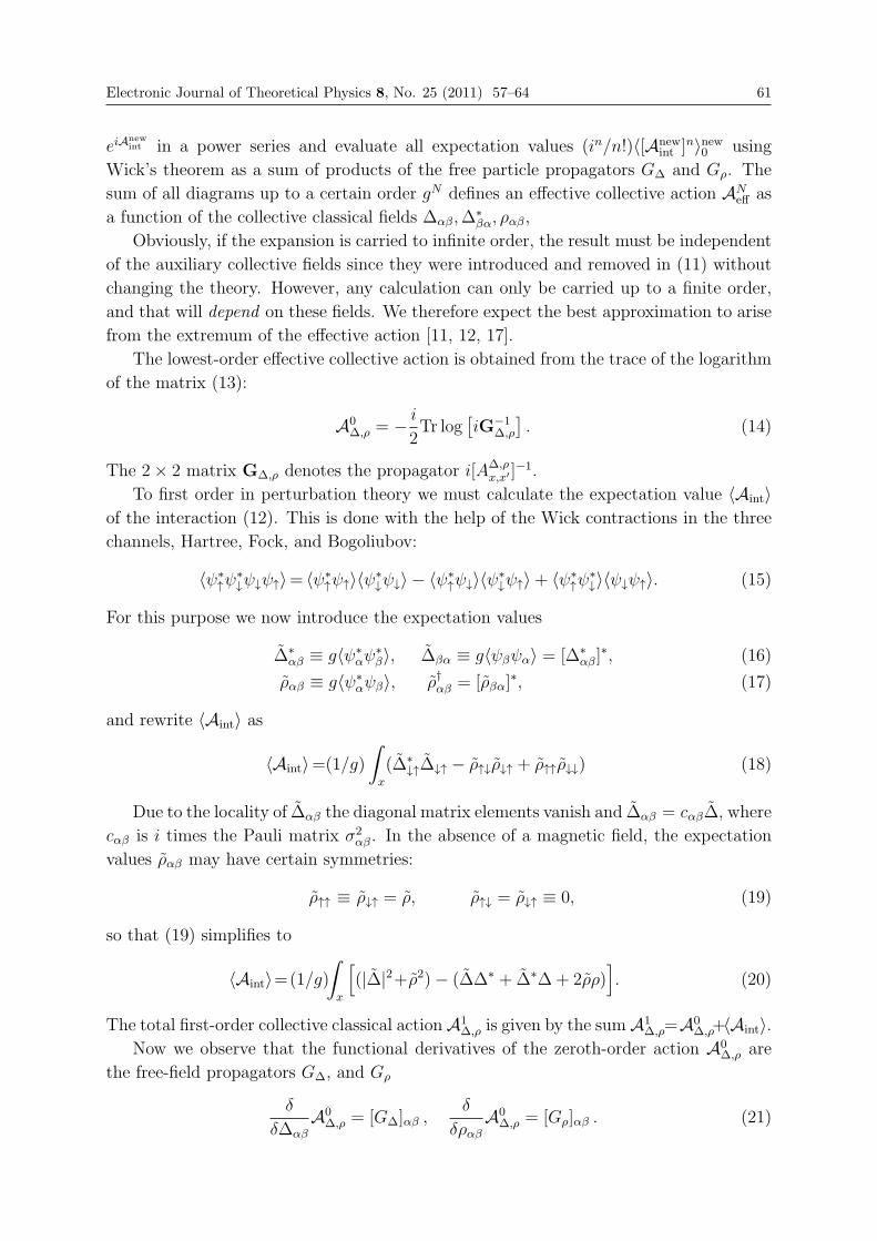
Electronic Journal of Theoretical Physics 8, No. 25 (2011) 57–64 61
eiAnewint in a power series and evaluate all expectation values (in/n!)〈[Anew
int ]n〉new0 using
Wick’s theorem as a sum of products of the free particle propagators GΔ and Gρ. The
sum of all diagrams up to a certain order gN defines an effective collective action ANeff as
a function of the collective classical fields Δαβ,Δ∗βα, ραβ,
Obviously, if the expansion is carried to infinite order, the result must be independent
of the auxiliary collective fields since they were introduced and removed in (11) without
changing the theory. However, any calculation can only be carried up to a finite order,
and that will depend on these fields. We therefore expect the best approximation to arise
from the extremum of the effective action [11, 12, 17].
The lowest-order effective collective action is obtained from the trace of the logarithm
of the matrix (13):
A0Δ,ρ = −
i
2Tr log
[iG−1
Δ,ρ
]. (14)
The 2× 2 matrix GΔ,ρ denotes the propagator i[AΔ,ρx,x′ ]
−1.To first order in perturbation theory we must calculate the expectation value 〈Aint〉
of the interaction (12). This is done with the help of the Wick contractions in the three
channels, Hartree, Fock, and Bogoliubov:
〈ψ∗↑ψ∗↓ψ↓ψ↑〉= 〈ψ∗↑ψ↑〉〈ψ∗↓ψ↓〉 − 〈ψ∗↑ψ↓〉〈ψ∗↓ψ↑〉+ 〈ψ∗↑ψ∗↓〉〈ψ↓ψ↑〉. (15)
For this purpose we now introduce the expectation values
Δ∗αβ ≡ g〈ψ∗αψ∗β〉, Δβα ≡ g〈ψβψα〉 = [Δ∗αβ]∗, (16)
ραβ ≡ g〈ψ∗αψβ〉, ρ†αβ = [ρβα]∗, (17)
and rewrite 〈Aint〉 as
〈Aint〉=(1/g)∫x
(Δ∗↓↑Δ↓↑ − ρ↑↓ρ↓↑ + ρ↑↑ρ↓↓) (18)
Due to the locality of Δαβ the diagonal matrix elements vanish and Δαβ = cαβΔ, where
cαβ is i times the Pauli matrix σ2αβ. In the absence of a magnetic field, the expectation
values ραβ may have certain symmetries:
ρ↑↑ ≡ ρ↓↑ = ρ, ρ↑↓ = ρ↓↑ ≡ 0, (19)
so that (19) simplifies to
〈Aint〉=(1/g)∫x
[(|Δ|2+ρ2)− (ΔΔ∗ + Δ∗Δ+ 2ρρ)
]. (20)
The total first-order collective classical actionA1Δ,ρ is given by the sumA1
Δ,ρ=A0Δ,ρ+〈Aint〉.
Now we observe that the functional derivatives of the zeroth-order action A0Δ,ρ are
the free-field propagators GΔ, and Gρ
δ
δΔαβ
A0Δ,ρ = [GΔ]αβ ,
δ
δραβA0
Δ,ρ = [Gρ]αβ . (21)

62 Electronic Journal of Theoretical Physics 8, No. 25 (2011) 57–64
Then we can extremize A1Δ,ρ with respect to Δ and ρ, and find that, to this order, the field
expectation values (17) are given by the free-field propagators (21) at equal arguments:
Δx = g[GΔ]x,x, ρx = g[Gρ]x,x. (22)
Thus we see that at the extremum, the action A1Δ,ρ is the same as the extremal action
A1[Δ, ρ] = A0[Δ, ρ]−1
g
∫x
(|Δ|2 + ρ2). (23)
Note how the theory differs, at this level, from the collective quantum field theory derived
via the HST. If we assume that ρ vanishes identically, the extremum of the one-loop action
A1[Δ, ρ] gives the same result as of the mean-field collective quantum field action (6),
which reads for the present δ-function attraction A1[Δ] = A0[Δ]− 1g
∫x|Δ|2. On the other
hand, if we extremize the action A1Δ,ρ at Δ = 0, we find the extremum from the expression
A1[Δ, ρ] = A0[Δ, ρ]− 1g
∫xρ2. The extremum of the first-order collective classical action
(23) agrees with the good-old Hartree-Fock-Bogolioubov theory.
The essential difference between this and the new approach arises in two ways:
• First when it is carried to higher orders. In the collective quantum field theory
based on the HST the higher-order diagrams must be calculated with the help of
the propagators of the collective field such as 〈ΔxΔx′〉. These are extremely compli-cated functions. For this reason, any loop diagram formed with them is practically
impossible to integrate. In contrast to that, the higher-order diagrams in the present
theory need to be calulated using only ordinary particle propagators GΔ and Gρ of
Eq. (21) and the interaction (12). Even that becomes, of course, tedious for higher
orders in g. At least, there is a simple rule to find the contributions of the quadratic
terms 12
∫xfTxMxfx in (11), given the diagrams without these terms. One calculates
the diagrams from only the four-particle interaction, and collects the contributions
up to order gN in an effective action AN [Δ, ρ]. Then one replaces AN [Δ, ρ] by
AN [Δ− εgΔ, ρ− εgρ] and re-expands everything in powers of g up to the order gN ,forming a new series
∑Ni=0 g
iAi[Δ, ρ]. Finally one sets ε equal to 1/g [15] and obtains
the desired collective classical action AN [Δ, ρ] as an expansion extending (23):
AN [Δ, ρ] =N∑i=0
Ai[Δ, ρ]− (1/g)
∫x
(|Δ|2 + ρ2). (24)
Note that this action must merely be extremized. There are no more quantum
fluctuations in the classical collective fields Δ, ρ. Thus, at the extremum, the action
(24) is directly the grand-canonical potential.
• The second essential difference with respect to the HST approach is that it is now
possible to study a rich variety of possible competing collective fields without the
danger of double-counting Feynman diagrams. One simply generalizes the matrix
Mx subtracted fromAint and added toAint in (11) in different ways. For instance, we
may subtract and add a vector field ψ†σaψSa containing the Pauli matrices σa and
study paramagnon fluctuations, thus generalizing the assumption (??) and allowing

Electronic Journal of Theoretical Physics 8, No. 25 (2011) 57–64 63
for a spontaneous magnetization in the ground state. Or one may do the same thing
with a term ψ†σa∇iψAia + c.c. in addition to the previous term, and derive the
Ginzburg-Landau theory of superfluid He3 as in [6].
An important property of the proposed procedure is that it yields good results in
the limit of infinitely strong coupling. It was precisely this property which led to the
successful calculation of critical exponents of all φ4 theories in the textbook [12] since
critical phenomena arise in the limit in which the unrenormalized coupling constant
goes to infinity [18]. This is in contrast to another possibility, in principle, of carrying
the variational approach to higher order via the so-called higher effective actions [19].
There one extremizes the Legendre transforms of the generating functionals of bilocal
correlation functions, which sums up all two-particle irreducible diagrams. That does
not give physically meaningful results [20] in the strong-coupling limit, even for simple
quantum-mechanical models.
6. The mother of this approach, Variational Perturbation Theory [11], is a systematic
extension of a variational method developed some years ago by Feynman and the author
[16]. It converts divergent perturbation expansions of quantum mechanical systems into
exponentially fast converging expansions for all coupling strength [17]. What we have
shown here is that this powerful theory can easily be transferred to many-body theory,
if we identfy a variety of relevant collective classical fields, rather than a fluctuating
collective quantum field suggested by the HST. This allows us to go systematically beyond
the standard Hartree-Fock-Bogoliubov approximation.
Acknowledgement
I am grateful to Flavio Nogueira, Aristieu Lima, and Axel Pelster for intensive discussions.
References
[1] R.L. Stratonovich, Sov. Phys. Dokl. 2, 416 (1958), J. Hubbard, Phys. Rev. Letters 3,77 (1959); B. Muhlschlegel, J. Math. Phys. 3, 522 (1962); J. Langer, Phys. Rev. 134,A 553 (1964); T. M. Rice, Phys. Rev. 140 A 1889 (1965); J. Math. Phys. 8, 1581(1967); A. V. Svidzinskij, Teor. Mat. Fiz. 9, 273 (1971); D. Sherrington, J. Phys. C4401 (1971).
[2] These identities were first employed in relativistic quantum field theory by P. T.Mathews, A. Salam, Nuovo Cimento 12, 563 (1954), 2, 120 (1955), and later instudies of the large-N limit of various model field theories, such as Gross-Neveu andnonlinear σ models.
[3] H. Kleinert, On the Hadronization of Quark Theories, Lectures presented at the EriceSummer Institute 1976, in Understanding the Fundamental Constituents of Matter,Plenum Press, New York, 1978, A. Zichichi ed., pp. 289-390 (klnrt.de/53/53.pdf).
[4] L.P. Gorkov, Sov. Phys. JETP 9, 1364 (1959). See also A.A. Abrikosov, L.P.Gorkov, I.E. Dzyaloshinski, Methods of Quantum Field Theory in Statistical Physics,Dover, New York (1975); L.P. Kadanoff, G. Baym, Quantum Statistical Mechanics,Benjamin, New York (1962); A. Fetter, J.D. Walecka, Quantum Theory of Many-Paricle Systems, McGraw-Hill, New York (1971).

64 Electronic Journal of Theoretical Physics 8, No. 25 (2011) 57–64
[5] V.L. Ginzburg and L.D. Landau, Eksp. Teor. Fiz. 20, 1064 (1950).
[6] H. Kleinert, Collective Quantum Fields, Lectures presented at the First Erice SummerSchool on Low-Temperature Physics, 1977, Fortschr. Physik 26, 565-671 (1978)(klnrt.de/55/55.pdf).
[7] E.H. Lieb, Int. J. Quantum Chem. 24, 243 (1983); R. Fukuda et al., Progr. Theor.Phys. 92, 833 (1994).
[8] R.G. Parr and W. Yang, Density Functional Theory of Atoms and Molecules, Oxford,Oxford, 1989; K.U. Gross and R.M. Dreizler, Density Functional Theory, NATOScience Series B, 1995.
[9] P. Hohenberg and W. Kohn, Phys. Rev. 136, B864 (1964)W. Kohn and L. J. Sham, Phys. Rev. 140, A1133 (1965).
[10] A. Leggett, Rev. Mod. Phys. 47, 331 (1975).
[11] H. Kleinert, Path Integrals in Quantum Mechanics, Statistics, Polymer Physics, andFinancial Markets, 5th ed., World Scientific, 2009 (klnrt.de/b8).
[12] H. Kleinert and V. Schulte-Frohlinde, Critical Properties of φ4-Theories, WorldScientific, 2001 (klnrt.de/b8).
[13] For more details see klnrt.de/b8/crit.htm).
[14] Note that the hermitian adjoint Δ∗↑↓ comprises transposition in the spin indices, i.e.,Δ∗↑↓ = [Δ↓↑]
∗.
[15] The alert reader will recognize her the so-called square-root trick of Chapter 5 in thetextbook Ref. [11].
[16] R.P. Feynman and H. Kleinert, Phys. Rev. A 34, 5080 (1986) (klnrt.de/159).
[17] H. Kleinert, Converting Divergent Weak-Coupling into Exponentially Fast ConvergentStrong-Coupling Expansions, Lecture presented at the Summer School on”Approximation and extrapolation of convergent and divergent sequences and series”in Luminy bei Marseille in 2009 (arXiv:1006.2910).
[18] H. Kleinert, Phys. Rev. D 57, 2264 (1998); Phys.Rev. D 60, 085001 (1999). (See alsoklnrt.de/critical).
[19] C. De Dominicis, J. Math. Phys. 3, 938 (1962); C. De Dominicis and P.C. Martin, J.Math. Phys. 5, 16, 31 (1964); J.M. Cornwall, R. Jackiw, and E.T. Tomboulis, Phys.Rev. D 10, 2428 (1974); H. Kleinert, Fortschr. Phys. 30, 187 (1982) (klnrt.de/82);Lett. Nuovo Cimento 31, 521 (1981) (klnrt.de/77).
[20] H. Kleinert, Annals of Physics 266, 135 (1998) (klnrt.de/255).

EJTP 8, No. 25 (2011) 65–82 Electronic Journal of Theoretical Physics
A Clarification on the Debate on “the OriginalSchwarzschild Solution”
Christian Corda∗
International Institute for Theoretical Physics and Mathematics Einstein-Galilei, viaSanta Gonda 14, Prato Italy
andInstitute for Basic Research, P. O. Box 1577, Palm Harbor, FL 34682, USA
Received 22 December 2010, Accepted 16 February 2011, Published 25 May 2011
Abstract: Now that English translations of Schwarzschild’s original paper exist, that paper has
become accessible to more people. Historically, the so-called ”standard Schwarzschild solution”
was not the original Schwarzschild’s work, but it is actually due to J. Droste and, independently,
H. Weyl, while it has been ultimately enabled like correct solution by D. Hilbert. Based on
this, there are authors who claim that the work of Hilbert was wrong and that Hilbert’s mistake
spawned black-holes and the community of theoretical physicists continues to elaborate on this
falsehood, with a hostile shouting down of any and all voices challenging them. In this paper
we re-analyse ”the original Schwarzschild solution” and we show that it is totally equivalent to
the solution enabled by Hilbert. Thus, the authors who claim that ”the original Schwarzschild
solution” implies the non existence of black holes give the wrong answer. We realize that the
misunderstanding is due to an erroneous interpretation of the different coordinates. In fact,
arches of circumference appear to follow the law dl = rdϕ, if the origin of the coordinate system
is a non-dimensional material point in the core of the black-hole, while they do not appear to
follow such a law, but to be deformed by the presence of the mass of the central body M if the
origin of the coordinate system is the surface of the Schwarzschild sphere.c© Electronic Journal of Theoretical Physics. All rights reserved.
Keywords: Black Holes; Schwarzschild solution; Singularity
PACS (2010): 04.70.-s; 04.70.Bw
1. Introduction
The concept of black-hole (BH) has been considered very fascinating by scientists even
before the introduction of general relativity (see [1] for an historical review). A BH is
a region of space from which nothing, not even light, can escape. It is the result of

66 Electronic Journal of Theoretical Physics 8, No. 25 (2011) 65–82
the deformation of spacetime caused by a very compact mass. Around a BH there is
an undetectable surface which marks the point of no return. This surface is called an
event horizon. It is called ”black” because it absorbs all the light that hits it, reflecting
nothing, just like a perfect black body in thermodynamics [2]. However, an unsolved
problem concerning such objects is the presence of a space-time singularity in their core.
Such a problem was present starting by the firsts historical papers concerning BHs [3, 4, 5].
It is a common opinion that this problem could be solved when a correct quantum gravity
theory will be, finally, obtained, see [6] for recent developments.
On the other hand, fundamental issues which dominate the question about the ex-
istence or non-existence of BH horizons and singularities and some ways to avoid the
development of BH singularities within the classical theory, which does not require the
need for a quantum gravity theory, have been discussed by various authors in the litera-
ture, see references from [7] to [16]. In fact, by considering the exotic nature of BHs, it
may be natural to question if such bizarre objects could exist in nature or to suggest that
they are merely pathological solutions to Einstein’s equations. Einstein himself thought
that BHs would not form, because he held that the angular momentum of collapsing
particles would stabilize their motion at some radius [17].
Recently, the debate became very hot as English translations of Schwarzschild’s orig-
inal work now exist and that work has become accessible to more people [18, 19]. Histor-
ically, the so-called ”Schwarzschild solution” was not the original Schwarzschild’s work,
but it is actually due to J. Droste [20] and, independently, H. Weyl [21], while it has been
ultimately enabled like correct solution by D. Hilbert [22]. Let us further clarify this point
by adding some historical notes. In 1915, A. Einstein developed his theory of general rel-
ativity [23]. A few months later, K. Schwarzschild gave the solution for the gravitational
field of a point mass and a spherical mass [3]. A few months after Schwarzschild, J. Droste,
a student of H. Lorentz, independently gave an apparently different solution for the point
mass and wrote more extensively about its properties [20]. In such a work Droste also
claimed that his solution was physically equivalent to the one by Schwarzschild. In the
same year, 1917, H. Weyl re-obtained the same solution by Droste [21]. This solution
had a peculiar behaviour at what is now called the Schwarzschild radius, where it became
singular, meaning that some of the terms in the Einstein equations became infinite. The
nature of this surface was not quite understood at the time, but Hilbert [22] claimed that
the form by Droste and Weyl was preferable to that in [3] and ever since then the phrase
“Schwarzschild solution” has been taken to mean the line-element which was found in
[20, 21] rather than the original solution in [3]. In 1924, A. Eddington showed that the
singularity disappeared after a change of coordinates (Eddington coordinates [24]), al-
though it took until 1933 for G. Lemaıtre to realize, in a series of lectures together with
Einstein, that this meant the singularity at the Schwarzschild radius was an unphysical
coordinate singularity [25].
In 1931, S. Chandrasekhar calculated that a non-rotating body of electron-degenerate
matter above 1.44 solar masses (the Chandrasekhar limit) would collapse [5]. His argu-
ments were opposed by many of his contemporaries like Eddington, Lev Landau and the

Electronic Journal of Theoretical Physics 8, No. 25 (2011) 65–82 67
same Einstein. In fact, a white dwarf slightly more massive than the Chandrasekhar
limit will collapse into a neutron star which is itself stable because of the Pauli exclusion
principle [1]. But in 1939, J. R. Oppenheimer and G. M. Volkoff predicted that neutron
stars above approximately 1.5 - 3 solar masses (the famous Oppenheimer–Volkoff limit)
would collapse into BHs for the reasons presented by Chandrasekhar, and concluded that
no law of physics was likely to intervene and stop at least some stars from collapsing
to BHs [26]. Oppenheimer and Volkoff interpreted the singularity at the boundary of
the Schwarzschild radius as indicating that this was the boundary of a bubble in which
time stopped. This is a valid point of view for external observers, but not for free-falling
observers. Because of this property, the collapsed stars were called ”frozen stars” [27]
because an outside observer would see the surface of the star frozen in time at the instant
where its collapse takes it inside the Schwarzschild radius. This is a known property of
modern BHs, but it must be emphasized that the light from the surface of the frozen
star becomes redshifted very fast, turning the BH black very quickly. Originally, many
physicists did not accept the idea of time standing still at the Schwarzschild radius, and
there was little interest in the subject for lots of time. But in 1958, D. Finkelstein, by
re-analysing Eddington coordinates, identified the Schwarzschild surface r = 2M (in nat-
ural units, i.e. G = 1, c = 1 and � = 1, i.e where r is the radius of the surface and M
is the mass of the BH) as an event horizon, ”a perfect unidirectional membrane: causal
influences can cross it in only one direction” [28]. This extended Oppenheimer’s results
in order to include the point of view of free-falling observers. Finkelstein’s solution ex-
tended the Schwarzschild solution for the future of observers falling into the BH. Another
complete extension was found by M. Kruskal in 1960 [29].
These results generated a new interest on general relativity, which, together with BHs,
became mainstream subjects of research within the Scientific Community. This process
was endorsed by the discovery of pulsars in 1968 [30] which resulted to be rapidly rotating
neutron stars. Until that time, neutron stars, like BHs, were regarded as just theoretical
curiosities; but the discovery of pulsars showed their physical relevance and spurred a
further interest in all types of compact objects that might be formed by gravitational
collapse.
In this period more general BH solutions were found. In 1963, R. Kerr found the
exact solution for a rotating BH [31]. Two years later E. T. Newman and A. Janis found
the asymmetric solution for a BH which is both rotating and electrically charged [32].
Through the works by W. Israel, B. Carter and D. C. Robinson the no-hair theorem
emerged [1], stating that a stationary BH solution is completely described by the three
parameters of the Kerr–Newman metric; mass, angular momentum, and electric charge
[1].
For a long time, it was suspected that the strange features of the BH solutions were
pathological artefacts from the symmetry conditions imposed, and that the singularities
would not appear in generic situations. This view was held in particular by Belinsky,
Khalatnikov, and Lifshitz, who tried to prove that no singularities appear in generic solu-
tions [1]. However, in the late sixties R. Penrose and S. Hawking used global techniques

68 Electronic Journal of Theoretical Physics 8, No. 25 (2011) 65–82
to prove that singularities are generic [1].
The term ”black hole” was first publicly used by J. A. Wheeler during a lecture in
1967 [33] but the first appearing of the term, in 1964, is due by A. Ewing in a letter
to the American Association for the Advancement of Science [34], verbatim: “According
to Einstein’s general theory of relativity, as mass is added to a degenerate star a sudden
collapse will take place and the intense gravitational field of the star will close in on itself.
Such a star then forms a ‘black hole’ in the universe.”
In any case, after Wheeler’s use of the term, it was quickly adopted in general use.
Today, the majority of researchers in the field is persuaded that there is no obstacle
to forming an event horizon. On the other hand, there are other researchers who demon-
strated that various physical mechanisms can, in principle, remove both of event horizon
and singularities during the gravitational collapse [7] - [16]. In particular, in [9] an exact
solution of Einstein field equations which removes both of event horizon and singularities
has been found by constructing the right-hand side of the field equations, i.e. the stress-
energy tensor, through a non-linear electrodynamics Lagrangian which was previous used
in super-strongly magnetized compact objects, such as pulsars, and particular neutron
stars [35, 36].
On the other hand, there are researchers who invoke the non existence of BH by
claiming that the Schwarzschild’s original work [3] gives a solution which is physically
different from the one derived by Droste [20] and Weyl [21]. Let us see this issue in more
detail. The new translations of Schwarzschild’s original work can be found in ref. [18, 19].
These works commented on Schwarzschild’s original paper [3]. In particular Abrams [18]
claimed that the line-element (we use natural units in all this paper)
ds2 = (1− rgr)dt2 − r2(sin2 θdϕ2 + dθ2)− dr2
1− rgr
(1)
i.e. the famous and fundamental solution to the Einstein field equations in vacuum, gives
rise to a space-time that is neither equivalent to Schwarzschild’s original solution in [3].
Abrams also claimed that Hilbert [22] opined that the form of (1) by Droste and Weyl
was preferable to that in [3] and ever since then the phrase “Schwarzschild solution”
has been taken to mean the line-element (1) rather than the original solution in [3].
In a following work [37] Abrams further claimed that “Black Holes are The Legacy of
Hilbert’s Error” as Hilbert’s derivation used a wrong variable. Thus, Hilbert’s assertion
that the form of (1) was preferable to the original one in [3] should be invalid. Based
on this, there are authors who agree with Abrams by claiming that the work of Hilbert
was wrong and Hilbert’s mistake spawned the BHs and the community of theoretical
physicists continues to elaborate on this falsehood, with a hostile shouting down of any
and all voices challenging them, see for example references [38, 39, 40, 41].
In this paper we re-analyse “the original Schwarzschild solution” to Einstein field equa-
tions derived in [3]. Such a solution arises from an apparent different physical hypothesis
which assumes arches of circumference to to do not follow the law dl = rdϕ, but to be
deformed by the presence of the mass of the central bodyM. This assumption enables the

Electronic Journal of Theoretical Physics 8, No. 25 (2011) 65–82 69
origin of the coordinate system to be not a single point, but a spherical surface having
radius equal to the gravitational radius, i.e. the surface of the Schwarzschild sphere. The
solution works for the external geometry of a spherical static star and circumnavigates
the Birkhoff theorem [4].
Then, the simplest case of gravitational collapse, i.e. the spherical radial collapse of a
star with uniform density and zero pressure, will be analysed by turning attention to the
interior of the collapsing object and the precise word line that its surface follows in the
external geometry. The result of the analysis will show that the singularity within the
totally collapsed spherical object remains. In fact, a coordinate transform that transfers
the origin of the coordinate system, which is the surface of a sphere having radius equal
to the gravitational radius, in a non-dimensional material point in the core of the BH re-
obtains the solution (1). Thus, “the original Schwarzschild solution” [3] results physically
equivalent to the solution (1) enabled like the correct on by Hilbert in [23], i.e. the solution
that is universally known like the ”Schwarzschild solution” [1]. This analysis ultimately
shows that the authors who claim that the original Schwarzschild solution leaves no room
for the science fiction of the BHs (see references[18, 19] and from [37] to [41]) give the
wrong answer. The misunderstanding is due to an erroneous interpretation of the different
coordinates. In fact, arches of circumference appear to follow the law dl = rdϕ, if the
origin of the coordinate system is a non-dimensional material point in the core of the
BH, while they do not appear to follow such a law, but to be deformed by the presence
of the mass of the central body M if the origin of the coordinate system is the surface of
the Schwarzschild sphere. Thus, the only way to remove the singularity in the core of a
BH within the classical theory of Einstein’s general relativity is changing the hypotheses
which govern the internal geometry of the collapsing star, following for example the ideas
in references from [7] to [16].
2. The “original Schwarzschild solution”
Following [42], the more general line-element which respects central symmetry is
ds2 = h(r, t)dr2 + k(r, t)(sin2 θdϕ2 + dθ2) + l(r, t)dt2 + a(r, t)drdt, (2)
where
r ≥ 0, 0 ≤ θ ≤ π, 0 ≤ ϕ ≤ 2π. (3)
We search a line-element solution in which the metric is spatially symmetric with
respect to the origin of the coordinate system, i.e. that we find again the same solution
when spatial coordinates are subjected to a orthogonal transformations and rotations and
it is asymptotically flat at infinity [1]. In order to obtain the “standard Schwarzschild
solution”, i.e. the line-element (1), to Einstein field equations in vacuum one uses trans-
formations of the type [42]
r = f1(r′, t′), t = f2(r
′, t′) , (4)

70 Electronic Journal of Theoretical Physics 8, No. 25 (2011) 65–82
where f1 and f1 are arbitrary functions of the new coordinates r′ and t′. At this point,if one wants the “standard Schwarzschild solution”, r and t have to be chosen in a way
that a(r, t) = 0 and k(r, t) = −r2 [42]. In particular, the second condition implies thatthe standard Schwarzschild radial coordinate is determined in a way which guarantees
that the length of the circumference centred in the origin of the coordinate system is 2πr
[42].
In our approach we will suppose again that a(r, t) = 0, but, differently from the
standard analysis, we will assume that the length of the circumference centred in the
origin of the coordinate system is not 2πr. We release an apparent different physical
assumption, i.e. that arches of circumference are deformed by the presence of the mass
of the central body M. Note that this different physical hypothesis permits to circum-
navigate the Birkhoff Theorem [4] which leads to the “standard Schwarzschild solution”
[3]. In fact, the demonstration of the Birkhoff Theorem starts from a line element in
which k(r, t) = −r2 has been chosen, see the discussion in paragraph 32.2 of [1] and, in
particular, look at Eq. (32.2) of such a paragraph.
Then, we proceed assuming k = −mr2, wherem is a generic function to be determined
in order to obtain that the length of circumferences centred in the origin of the coordinate
system are not 2πr. In other words, m represents a measure of the deviation from 2πr
of circumferences centred in the origin of the coordinate system.
The line element (2) becomes
ds2 = hdr2 −mr2(sin2 θdϕ2 + dθ2) + ldt2. (5)
One puts
X ≡ 13r3
Y ≡ − cos θ
Z ≡ ϕ.
(6)
In the X, Y, Z coordinates the line-element (5) reads
ds2 = ldt2 +hr4dX2 −mr2[
dY 2
1− Y 2+ dZ2(1− Y 2)]. (7)
Let us consider three functions

Electronic Journal of Theoretical Physics 8, No. 25 (2011) 65–82 71
A ≡ − hr4
B ≡ mr2
C ≡ l
(8)
which satisfy the conditions
X →∞ implies A→ 1r4= 1
(3X)43, B → r2 = 3X
23 , C → 1
normalization condition AB2C = 1.
(9)
The line-element (7) becomes
ds2 = Cdt2 − AdX2 −BdY 2
1− Y 2−BdZ2(1− Y 2). (10)
From the metric (10) one gets the Christoffell coefficients like (only the non zero
elements will be written down)
ΓttX = − 1
2C∂C∂X
ΓXXX = − 1
2A∂A∂X
ΓXY Y = 1
2A∂B∂X
11−Y 2 ΓX
ZZ =12A
∂B∂X(1− Y 2)
ΓXtt = − 1
2A∂C∂X
ΓYY X = − 1
2B∂B∂X
ΓYY Y = −Y
1−Y 2 ΓYZZ = −Y (1− Y 2)
ΓZZX = − 1
2B∂B∂X
ΓZZX = Y
1−Y 2 .
(11)
By using the equation for the components of the Ricci tensor, the components of
Einstein field equation in vacuum are [42]
Rik =∂Γl
ik
dxl− ∂Γl
il
dxk− Γl
ikΓmlm − Γm
il Γlkm = 0. (12)
By inserting Eqs. (11) in Eqs. (12) one gets only three independent relations
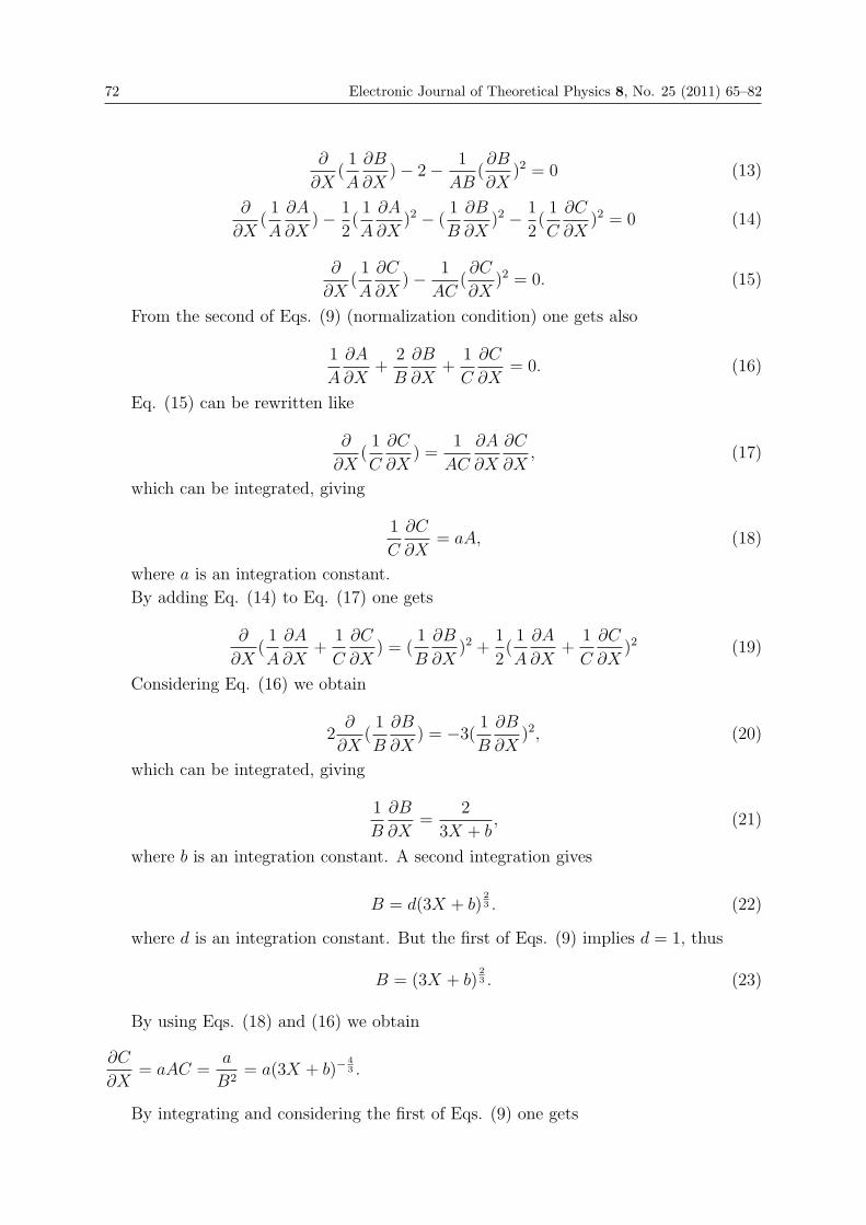
72 Electronic Journal of Theoretical Physics 8, No. 25 (2011) 65–82
∂
∂X(1
A
∂B
∂X)− 2− 1
AB(∂B
∂X)2 = 0 (13)
∂
∂X(1
A
∂A
∂X)− 1
2(1
A
∂A
∂X)2 − (
1
B
∂B
∂X)2 − 1
2(1
C
∂C
∂X)2 = 0 (14)
∂
∂X(1
A
∂C
∂X)− 1
AC(∂C
∂X)2 = 0. (15)
From the second of Eqs. (9) (normalization condition) one gets also
1
A
∂A
∂X+
2
B
∂B
∂X+
1
C
∂C
∂X= 0. (16)
Eq. (15) can be rewritten like
∂
∂X(1
C
∂C
∂X) =
1
AC
∂A
∂X
∂C
∂X, (17)
which can be integrated, giving
1
C
∂C
∂X= aA, (18)
where a is an integration constant.
By adding Eq. (14) to Eq. (17) one gets
∂
∂X(1
A
∂A
∂X+
1
C
∂C
∂X) = (
1
B
∂B
∂X)2 +
1
2(1
A
∂A
∂X+
1
C
∂C
∂X)2 (19)
Considering Eq. (16) we obtain
2∂
∂X(1
B
∂B
∂X) = −3( 1
B
∂B
∂X)2, (20)
which can be integrated, giving
1
B
∂B
∂X=
2
3X + b, (21)
where b is an integration constant. A second integration gives
B = d(3X + b)23 . (22)
where d is an integration constant. But the first of Eqs. (9) implies d = 1, thus
B = (3X + b)23 . (23)
By using Eqs. (18) and (16) we obtain
∂C
∂X= aAC =
a
B2= a(3X + b)−
43 .
By integrating and considering the first of Eqs. (9) one gets

Electronic Journal of Theoretical Physics 8, No. 25 (2011) 65–82 73
C = 1− a(3X + b)−13 (24)
Then, from Eq. (16) one obtains
A =(3X + b)−
43
1− a(3X + b)−13
. (25)
By putting Eqs. (25) and (23) in Eq. (13) one immediately sees that this last equation
is automatically satisfied.
We note that the function A results singular for values a(3X + b)−13 = 1. However,
this is a mathematical singularity due to the particular coordinates t,X, Y, Z defined by
the transformation (6). In fact, by assuming that such a singularity is located at X = 0
we get
b = a3, (26)
i.e. we find a relation between the two integration constants b and a.
At the end we obtain
A = (r3 + a3)−43 [1− a(r3 + a3)−
13 ]−1
B = (r3 + a3)23
C = 1− a(r3 + a3)−13 .
(27)
By inserting the functions (27) in Eq. (10) and using Eqs. (8) and (6) to return to
the standard polar coordinates the line-element solution reads
ds2 =
[1− a
(r3+a3)13
]dt2 − (r3 + a3)
23 (sin2 θdϕ2 + dθ2)+
− d(r3+a3)23
1− a
(r3+a3)13
.
(28)
Hence, we understand that the assumption to locate the mathematical singularity
of the function A at X = 0 coincides with the physical condition that the length of
the circumference centred in the origin of the coordinate system is 2π(r3 + a3)13 , which
is different from the value 2πr. This is the apparent fundamental physical difference
between this solution and the “standard Schwarzschild solution” (1), i.e. the one enabled
by Hilbert in [22]. The value of the generic function m which permits that the length of
circumferences centred in the origin of the coordinate system are not 2πr is
m =(r3 + a3)
23
r2. (29)

74 Electronic Journal of Theoretical Physics 8, No. 25 (2011) 65–82
On the other hand, in order to determinate the value of the constant a, by following
[42], one can use the weak field approximation which implies g00 ∼= 1 + 2ϕ at large
distances, where g00 = (1− a
(r3+a3)13) in Eq. (28) and ϕ ≡ −M
ris the Newtonian potential.
Thus, for a � r, we immediately obtain: a = 2M = rg, i.e. a results exactly the
gravitational radius [1, 42].
Then, we can rewrite the solution (28) in an ultimate way like
ds2 =
[1− rg
(r3+r3g)13
]dt2 − (r3 + r3g)
23 (sin2 θdϕ2 + dθ2)+
− d(r3+r3g)23
1− rg
(r3+r3g)13
.
(30)
Historically, the line-element (30) represents “the original Schwarzschild solution” to
Einstein field equations as it has been derived for the first time by Karl Schwarzschild in
[3] with a slight different analysis.
Some comments are needed. By looking Eq. (30) one understands that the origin
of the coordinate that we have chosen by putting r ≥ 0, 0 ≤ θ ≤ π 0 ≤ ϕ ≤ 2π and
with the additional assumption that the length of circumferences centred in the origin of
the coordinate system are not Euclidean, is not a single point, but it is the surface of a
sphere having radius rg, i.e. the surface of the Schwarzschild sphere. By putting
r ≡ (r3 + r3g)13 , (31)
Eq. (28) becomes
ds2 = (1− rgr)dt2 − r2(sin2 θdϕ2 + dθ2)− dr2
1− rgr
. (32)
Eq. (32) looks formally equal to the “standard Schwarzschild solution” (1). But one
could think that the transformation (31) is forbidden for the following motivation. It
transfers the origin of the coordinate system, r = 0, θ = 0, ϕ = 0, which is the surface
of a sphere having radius rg in the r, θ, ϕ coordinates, in a non-dimensional material
point r = 0, θ = 0, ϕ = 0 in the r, θ, ϕ coordinates. Such a non-dimensional material
point corresponds to the point r = −rg, θ = 0, ϕ = 0 in the original r, θ, ϕ coordinates.
Thus, the transformation (31) could not be a suitable coordinate transformation because
it transfers a spherical surface, i.e. a bi-dimensional manifold, in a non-dimensional
material point. We will see in the following that this interpretation is not correct.
On the other hand, we are searching a solution for the external geometry, thus we
assumed r ≥ 0 in Eq. (3) and from Eq. (31) it is always r ≥ rg in Eq. (32) as it is r ≥ 0
in Eq. (30). In this way, there are not physical singularities in Eq. (32). In fact, r = 0 in
Eq. (30) implies r = rg in Eq. (32) which corresponds to the mathematical singularity at
X = 0. This singularity is not physical but is due to the particular coordinates t,X, Y, Z
defined by the transformation (6).

Electronic Journal of Theoretical Physics 8, No. 25 (2011) 65–82 75
Again, we emphasize the apparent different assumption of our analysis. As it is
carefully explained in [42], the “standard Schwarzschild solution” (1), arises from the
hypothesis that the coordinates r and t of the two functions (4) are chosen in order to
guarantee that the length of the circumference centred in the origin of the coordinate
system is 2πr. Indeed, in the above derivation of “the original Schwarzschild solution”
(30), r and t are chosen in order to guarantee that the length of the circumference
centred in the origin of the coordinate system is not 2πr. In particular, choosing to put
the mathematical singularity of the function A at X = 0 is equivalent to the physical
condition that the length of the circumference centred in the origin of the coordinate
system is 2π(r3 + r3g)13 . Then, one could think that by forcing the transformation (31)
for r ≤ 0, one returns to the standard Schwarzschild solution (1), but a bi-dimensional
spherical surface, that is the surface of the Schwarzschild sphere, is forced to become a
non-dimensional material point and we force a non-Euclidean geometry for circumferences
to become Euclidean. In that case, such a mathematical forcing could be the cause of the
singularity in the core of the black-hole. Thus, this singularity could be only mathematical
and not physical. But in the following, by matching with the internal geometry, we will
see that this interpretation is not correct and that the singularity in the core of the BH
remains a physical singularity also in the case of the “original Schwarzschild solution”
given by Eq. (30).
Notice that a large distances, i.e. where rg � r, the solution (30) well approximates
the standard Schwarzschild solution (1), thus, both of the weak field approximation and
the analysis of astrophysical situations remain the same.
3. Matching with the internal geometry: singular gravitational
collapse
In the following we adapt the classical analysis in [1] to the line-element (30). Let us
consider a test particle moving in the external geometry (30). By following the magnitude
of the 4-vector of energy-momentum is represented by the rest mass μ of the particle [1]
gikpipk + μ2 = gikpipk + μ2 = 0, (33)
or
− E2
1− rg
(r3+r3g)13
+1
1− rg
(r3+r3g)13
r4
(r3 + r3g)43
(dr
dλ
)2
+L2
(r3 + r3g)23
+ μ2, (34)
where λ = τ/μ, L and E represent the affine parameter being τ the proper time, the
angular momentum and the energy of the particle [1].
Einstein equivalence principle [1] implies that test particles follow the same wordlines
regardless of mass. Then, what is relevant for the motion of particles are the normalized
quantities L = L/μ and E = E/μ.
Thus, Eq. (34) can be rewritten as

76 Electronic Journal of Theoretical Physics 8, No. 25 (2011) 65–82
(drdτ
)2=
(r3+r3g)43
r4
{E2 −
(1− rg
(r3+r3g)13
)(1 + L2
(r3+r3g)23
)}=
=(r3+r3g)
43
r4
(E2 − V 2(r)
),
(35)
where the “effective potential” is defined by
V (r) ≡
√√√√(1− rg
(r3 + r3g)13
)(1 +
L2
(r3 + r3g)23
). (36)
From Eq. (35) the proper time can be explicitly written down
τ =
ˆdτ =
ˆ ⎡⎣ dr(E2 − V 2(r)
) r2
(r3 + r3g)23
⎤⎦ . (37)
In the following we discuss the collapse of a star with uniform density and zero pres-
sure. Because no pressure gradients are present to deflect their motion, the particles on
the surface of any ball of dust must move along radial geodesic in the external geometry
of Eq. (30). The angular momentum vanishes and the integral (37) reduces to
τ =
ˆdτ =
ˆ⎡⎢⎢⎢⎢⎣ dr√(
rg
(r3+r3g)13− rg
(R3+r3g)13
) r2
(r3 + r3g)23
⎤⎥⎥⎥⎥⎦ , (38)
where R ≡ rg1−E2 is the “apastron”, i.e. the radius at which the particle has zero
velocity [1].
Eq. (38) can be integrated in parametric form:
r =1
2
[(R3 + r3g)(1 + cos η)3 − r3g
] 13 (39)
and
τ =(R3 + r3g)
13
2
(R3 + r3grg
) 16
(η + sin η). (40)
Eq. (40) is the proper time read by a clock on the surface of the collapsing star.
The collapse begins when the parameter η is zero (r = R, τ = 0) and terminates, for
the external geometry, at r = 0, η = 2rg
(R3+r3g)13−1
.
Thus, the total proper time to fall from rest at r = R into the surface of the sphere
r = 0 is

Electronic Journal of Theoretical Physics 8, No. 25 (2011) 65–82 77
τ =(R3 + r3g)
13
2
(R3 + r3grg
) 16
[arccos(
2rg
(R3 + r3g)13 − 1
) + sin arccos(2rg
(R3 + r3g)13 − 1
)
].
(41)
Let us focus the attention on the simplest ball of dust, an interior that is homogeneous
and isotropic everywhere, except at the surface. This is exactly the case of an interior
locally identical to a dust filled Friedmann closed cosmological model [1, 9]. In fact, the
closed model is the only one of interest because it corresponds to a gas sphere whose
dynamics begins at rest with a finite radius [1, 9]. The ordinary line-element is given by
[1, 9]
ds2 = −dτ 2 + a(τ)(+dχ2 + sin2 χ(dθ2 + sin2 θdϕ2), (42)
where a(τ) is the scale factor of the internal space-time. In the case of zero pressure
the stress-energy tensor is
T = ρu⊗ u, (43)
where ρ is the density of the star and u the 4-vector velocity of the matter. Thus, the
Einstein field equations give only one meaningful relation in terms of η [1, 9]
(da
dη)2 + a2 =
ρ
3a4, (44)
which admits the familiar cycloidal solution [1, 9]
a =a02(1 + cos η), (45)
and
τ =a02(η + sin η). (46)
where a0 is a constant.
Homogeneity and isotropy are broken only at the star’s surface which lies at a radius
χ = χ0 for all τ during the collapse [1, 9], as measured in terms of the co-moving hyper-
spherical polar angle χ. The match between the internal solution given by Eqs. (45) and
(46) and the external solution given by Eqs. (39) and (40) is possible. As a verification
of such a match let us examine the separate and independent predictions made by the
internal and external solutions for the star’s circumference [1]. From Eqs. (39) and (40)
the external solution enables the relations:
C = 2π(r3 + r3g)13 = 2π(R3 + r3g)
13 (1 + cos η)
τ =(R3+r3g)
13
2
(R3+r3g
rg
) 16(η + sin η).
(47)
From Eqs. (45) and (46) the internal solution enables the relations:

78 Electronic Journal of Theoretical Physics 8, No. 25 (2011) 65–82
C = 2π(r3 + r3g)13 = 2π a0 sinχ0
2(1 + cos η)
τ = a02(η + sin η).
(48)
Thus, the match works for all time during the collapse if and only if
R =(a30 sin
3 χ0 − r3g) 1
3
rg = a0 sin3 χ0.
(49)
By inserting the first of Eqs. (49) in Eq. (39) one gets
r =1
2
{[(a0 sinχ0)(1 + cos η)]3 − r3g
} 13 . (50)
Eq. (50) represents the run of the collapse for both the external and internal solu-
tions for 0 ≤ η ≤ 2rg
(R3+r3g)13−1
. When η = 2rg
(R3+r3g)13−1
it is r = 0 and particles reach the
Schwarzschild sphere which is the origin of the coordinate system. For η > 2rg
(R3+r3g)13−1
Eq. (50) represents only the trend of the internal solution and the r coordinate becomes
negative (this is possible because the origin of the coordinate system is the surface of the
Schwarzschild sphere). The r coordinate reaches a minimum r = −rg for η = π. Thus,
we understand that at this point the collapse terminates and the star is totally collapsed
in a singularity at r = −rg. In other terms, in the internal geometry all time-like radial
geodesics of the collapsing star terminate after a lapse of finite proper time in the ter-
mination point r = −rg and it is impossible to extend the internal space-time manifold
beyond that termination point. Thus, the point r = −rg represents a singularity basedon the rigorous definition by Schmidt [43].
Clearly, as all the particle of the collapsing star fall in the singularity at r = −rgvalues of r > −rg do not represent the internal geometry after the end of the collapse,
but they will represent the external geometry. This implies that the external solution
(30), i.e. “the original Schwarzschild solution” to Einstein field equations which has been
derived for the first time by Karl Schwarzschild in [3] can be analytically continued for
values of −rg < r ≤ 0 and it results physically equivalent to the solution (1) that is
universally known like the ”Schwarzschild solution”. In fact, now the transformation
(31) can be enabled and the origin of the coordinate system, r = 0, θ = 0, ϕ = 0, which
is the surface of a sphere having radius rg in the r, θ, ϕ coordinates, results transferred
in a non-dimensional material point r = 0, θ = 0, ϕ = 0 in the r, θ, ϕ coordinates. Such
a non-dimensional material point corresponds to the point r = −rg, θ = 0, ϕ = 0 in the
original r, θ, ϕ coordinates.
Then, the authors who claim that “the original Schwarzschild solution” leaves no
room for the science fiction of the BHs, see [18, 19], [37] - [41], give the wrong answer.

Electronic Journal of Theoretical Physics 8, No. 25 (2011) 65–82 79
We realize that the misunderstanding is due to an erroneous interpretation of the differ-
ent coordinates. In fact, arches of circumference appear to be 2πr if the origin of the
coordinate system is a non-dimensional material point in the core of the BH while they
do not appear to be 2πr, but deformed by the presence of the mass of the central body
M if the origin of the coordinate system is the surface of the Schwarzschild sphere.
The only way to remove the singularity in the core of a BH within the classical
theory of Einstein’s general relativity is changing the hypotheses which govern the internal
geometry of the collapsing star, following for example the ideas in references from [7] to
[16].
4. Conclusion remarks
In this paper we clarified a issue on the the debate on “the original Schwarzschild solu-
tion”. As English translations of Schwarzschild’s original paper exist, that paper has be-
come accessible to more people. A misunderstanding arises from the fact that, historically,
the so-called ”standard Schwarzschild solution” (1) was not the original Schwarzschild’s
work, but it is actually due to Droste [20] and Weyl [21]. The solution in refs. [20, 21]
has been ultimately enabled like correct solution by Hilbert in [22]. Based on this, there
are authors who claim that the work of Hilbert was wrong and that Hilbert’s mistake
spawned BHs and accuse the community of theoretical physicists to continue to elaborate
on this falsehood, with a hostile shouting down of any and all voices challenging them
[18, 19], [37] - [41].
With the goal to clarify the issue, we re-analysed “the original Schwarzschild solu-
tion” to Einstein field equations by showing that such a solution arises from an apparent
different physical hypothesis which assumes arches of circumference to be not 2πr, but
deformed by the presence of the mass of the central bodyM. This assumption enables the
origin of the coordinate system to be not a single point, but a spherical surface having
radius equal to the gravitational radius, i.e. the surface of the Schwarzschild sphere. The
solution works for the external geometry of a spherical static star and circumnavigates
the Birkhoff theorem. After this, we discussed the simplest case of gravitational collapse,
i.e. the spherical radial collapse of a star with uniform density and zero pressure, by
turning attention to the interior of the collapsing object and the precise word line that
its surface follows in the external geometry. The result is that the singularity within the
totally collapsed spherical object remains. In fact, a coordinate transform that transfers
the origin of the coordinate system, which is the surface of a sphere having radius equal to
the gravitational radius, in a non-dimensional material point in the core of the black-hole,
re-obtains the solution re-adapted by Hilbert. Thus, “the original Schwarzschild solution”
[3] results physically equivalent to the solution enabled by Hilbert in [22], i.e. the solution
that is universally known like ”the standard Schwarzschild solution”. We conclude that
Hilbert was not wrong but they are definitively wrong the authors who claim that “the
original Schwarzschild solution” implies the non existence of BHs [18, 19], [37] - [41]. The
misunderstanding is due to an erroneous interpretation of the different coordinates. In

80 Electronic Journal of Theoretical Physics 8, No. 25 (2011) 65–82
fact, arches of circumference appear to be 2πr if the origin of the coordinate system is a
non-dimensional material point in the core of the black-hole, while they do not appear
to be 2πr, but deformed by the presence of the mass of the central body M if the origin
of the coordinate system is the surface of the Schwarzschild sphere.
Therefore, the only way to remove the singularity in the core of a BH within the
classical theory of Einstein’s general relativity is changing the hypotheses which govern
the internal geometry of the collapsing star, following for example the ideas in references
from [7] to [16].
Acknowledgements
I thank Herman Mosquera Cuesta and Jeremy Dunning Davies for interesting discus-
sions on Black Hole physics. I also thank Chrysostomos for correcting typos in previous
versions of this paper. The R. M. Santilli Foundation has to be thanked for partially
supporting this paper (Research Grant of the R. M. Santilli Foundation Number RMS-
TH-5735A2310).
References
[1] C. W. Misner, K. S. Thorne and J. A. Wheeler, Gravitation, W. H. Freeman andCompany (1973).
[2] P. C. W. Davies, Rep. Prog. Phys. 41, 1313–1355 (1978).
[3] K. Schwarzschild, Sitzungsber. Preuss. Akad. Wiss. Berlin (Math. Phys.) 1916, 189-196 (1916).
[4] G. D. Birkhoff, Relativity and Modern Physics. Cambrigdge, MA: Harvard UniversityPress. LCCN 23008297 (1923).
[5] S. Chandrasekhar, The Highly Collapsed Configurations of a Stellar Mass, Mont.Not. Roy. Astr. Soc. 91, 456–466 (1931).
[6] H. Nicolai, G. F. R. Ellis, A. Ashtekar and others, Gen. Rel. Grav. 41, 4, 673-1011,Special Issue on quantum gravity (April 2009).
[7] S. Robertson and D. Leiter, Mon. Roy. Astron. Soc. 50, 1391 (2004).
[8] R. Schild, D. Leiter and S. Robertson, Astron. J. 2, 420-432 (2006).
[9] C. Corda and H. J. Mosquera Cuesta, Mod. Phys. Lett A 25, 28, 2423-2429 (2010).
[10] A. Mitra, Phys. Rev. Lett. 81, 4774 (1998).
[11] A. Mitra, Phys. Rev. D, 74, 2, 024010 (2006).
[12] A. Mitra, Mon. Not. Roy. Astron. Soc. 369, 492 (2006).
[13] A. Mitra, Journ. Math. Phys. 50, 4, 042502-042503 (2009).
[14] J. P. S. Lemos, O.B. Zaslavskii, arXiv:1004.4651 (2010).
[15] A. G. Agnese and M. La Camera, Phys. Rev. D 31, 1280–1286 (1985).

Electronic Journal of Theoretical Physics 8, No. 25 (2011) 65–82 81
[16] S. Robertson and D. Leiter, Astrophys. J. 596, L203-L206 (2003).
[17] A. Einstein, Ann. Math. 40, 4, 922–936 (1939).
[18] L. S. Abrams, Phys. Rev. D20, 2474 (1979), also in arXiv:gr-qc/0201044.
[19] S. Antoci and D.E. Liebscher, Gen. Rel. Grav. 35, 5, 945-950 (2003).
[20] J. Droste, Proc. K. Ned. Akad. Wet. 19, 197 (1917).
[21] H. Weyl, Ann. Phys. (Leipzig) 54, 117 (1917).
[22] D. Hilbert, Nachr. Ges. Wiss. G¨ttingen, Math. Phys. Kl., 53 (1917).
[23] A. Einstein, “Zur allgemeinen Relativitatstheorie”, Sitzungsberichte der a KoniglichPreußischen Akademie der Wissenschaften 1915, 778-86 (1915).
[24] A. S. Eddington, Nature 113, 192 (1924).
[25] A. Einstein and G. Lemaıtre, TALKING OVER THE UNIVERSE AND ITSORIGIN, Lectures in Pasadena, California, JWC-CX 1-13-33 [January 13, 1933] WCMET. (STAMPED JAN 14 1933).
[26] J. R. Oppenheimer and G. M. Volkoff, Phys. Rev. 55, 4, 374–381 (1939).
[27] R. Ruffini and J. A. Wheeler, Phys. Tod. 30–41 (1971).
[28] D. Finkelstein, Phys. Rev. 110, 965–967 (1958).
[29] M. Kruskal, Phys. Rev. 119, 1743–1745 (1960).
[30] A. Hewish, S. J. Bell and J. D. H Pilkington, Nature 217, 709–713 (1968).
[31] R. Kerr, Phys. Rev. Lett. 11, 237–238 (1963).
[32] E. T. Newman and A. Janis, Journ. Math. Phys. 6, 6, 915–917 (1965).
[33] S. Hawking, A Brief History of Time, Bantam Dell Publishing Group (1988).
[34] A. Ewing, Science News Letter of 18 (January 1964).
[35] H. J. Mosquera Cuesta and J. M. Salim, Mont. Not. Roy. Ast. Soc. 354, L55-L59(2004).
[36] H. J. Mosquera Cuesta and J. M. Salim, Ap. J. 608, 925-929 (2004).
[37] L. S. Abrams, Can. J. Phys. 67, 919 (1989), also in arXiv:gr-qc/0102055.
[38] S. Antoci, in ”Meteorological and Geophysical Fluid Dynamics (a book tocommemorate the centenary of the birth of Hans Ertel)”, W. Schroder Editor, ScienceEdition, Bremen, 2004 , also in arXiv:physics/0310104.
[39] S. J. Crothers, Prog. in Phys. Vol. 1 (2005).
[40] S. J. Crothers, Prog. in Phys. Vol. 2 (2005).
[41] A. Loinger and T. Marsico, Spacetime & Substance, No. 2 (17) (2003).
[42] L. Landau L and E. Lifshitz - Classical Theory of Fields (3rd ed.). London: Pergamon.ISBN 0-08-016019-0. Vol. 2 of the Course of Theoretical Physics (1971).
[43] B. G. Schmidt, Gen. Rel. Grav. 1, 269-280 (1971).


EJTP 8, No. 25 (2011) 83–92 Electronic Journal of Theoretical Physics
Entropy for Black Holes in the DeformedHorava-Lifshitz Gravity
Andres Castillo and Alexis Larranaga∗
Universidad Nacional de Colombia. Departamento de FısicaUniversidad Nacional de Colombia. Observatorio Astronomico Nacional
(OAN),Universidad Distrital Francisco Jose de Caldas. Facultad de Ingenierıa
Received 6 July 2010, Accepted 10 February 2011, Published 25 May 2011
Abstract: We study the entropy of black holes in the deformed Horava-Lifshitz gravity with
coupling constant λ. For λ = 1, the black hole resembles the Reissner-Nordstrom black hole
with a geometric parameter acting like the electric charge. Therefore, we obtain some differences
in the entropy when comparing with the Schwarzschild black hole. Finally, we study the heat
capacity and the thermodynamical stability of this solution.c© Electronic Journal of Theoretical Physics. All rights reserved.
Keywords: Physics of Black Holes; Thermodynamics; Modified Theories of Gravity
PACS (2010): 04.70.-s; 04.70.Dy; 04.50.Kd
1. Introduction
Recently, Horava [1] proposed a non-relativistic renormalisable theory of gravity that
reduces to Einstein’s general relativity at large scales. This theory is named Horava-
Lifshitz theory and has been studied in the literature for its applications to cosmology
[2] and black holes [3]. However, this proposal introduces back a non-equality of space
and time. Therefore, in this approach, space and time exhibit Lifshitz scale invariance
t → lzt and xi → lxi with z ≥ 1. Moreover, the theory is not invariant under the full
diffeomorphism group of General Relativity (GR), but rather under a subgroup of it.
This fact is manifest using the standard ADM splitting.
However, the Horava-Lifshitz theory goes to standard GR if the coupling λ that
controls the contribution of the trace of the extrinsic curvature has the specific value
λ = 1. For generic values of λ, the theory does not exhibits the full 4D diffeomorphism
invariance at large distances and it is possible to obtain deviations from GR. Therefore,

84 Electronic Journal of Theoretical Physics 8, No. 25 (2011) 83–92
it is interesting to confront this type of non-relativistic theory with experimental and
observational data.
Using the (3 + 1)-dimensional ADM formalism, the general metric can be written as
ds2 = −N2dt2 + gij(dxi +N idt)(dxj +N jdt) (1)
where gij, N and N i are the dynamical fields of scaling mass dimensions 0, 0, 2,
respectively. The Einstein-Hilbert action can be expressed as
SEH =1
16πG
∫d4x√gN{
(KijK
ij −K2)+R− 2Λ}, (2)
where G is Newton’s constant and the extrinsic curvature Kij takes the form
Kij =1
2N(gij −∇iNj −∇jNi) (3)
with a dot denoting derivative with respect to t and covariant derivatives defined with
respect to the spatial metric gij. On the other hand, the action of Horava-Lifshitz theory
is given by [1]
SHL =
∫dtd3x
√gN
[2
κ2(KijK
ij − λK2)+κ2μ2(ΛR− 3Λ2)
8(1− 3λ)+κ2μ2(1− 4λ)
32(1− 3λ)R2
−κ2μ2
8RijR
ij +κ2μ
2ω2εijkRil∇jR
lk −
κ2
2ω4CijC
ij
], (4)
where κ2, λ, ω are dimensionless constant parameters while μ and Λ are constant
parameters with mass dimensions [μ] = 1, [Λ] = 2. The object Cij is called the Cotten
tensor, defined by
Cij = εijk∇kRjl −
1
4εijk∂kR. (5)
Comparing the action to that of general relativity, one can see that the speed of light,
Newton’s constant and the cosmological constant are
c =κ2μ
4
√Λ
1− 3λ(6)
G =κ2c
32π(7)
Λ =3
2Λ. (8)
Note that if λ = 1, the first two terms in (4) could be reduced to the Einstein’s general
relativity action (2). However, in Horava-Lifshitz theory, λ is a dynamical coupling
constant, susceptible to quantum correction.
The static, spherically symmetric solutions have been found in [3]. Because of the
presence of a cosmological constant, solutions for λ = 1 are asymptotically AdS and have

Electronic Journal of Theoretical Physics 8, No. 25 (2011) 83–92 85
some interest because the AdS/CFT correspondence. These solutions have also been
extended to general topological black holes[4], in which the 2-sphere that acts as horizon
has been generalized to two dimensional constant curvature spaces.
2. Horava-Lifshitz Black Hole
Now we will introduce the black hole solution in the limit of Λ→ 0 and its thermodynamic
properties. Considering Ni = 0 (spherically symmetric solutions) in (1) we obtain the
metric ansatz
ds2 = −N2(r)dt2 +dr2
f(r)+ r2d2Ω. (9)
Using this line element and after the angular integration, the Lifshitz-Horava la-
grangian reduces to
L1 =κ2μ2N
8(1− 3λ)√f
(λ− 1
2f ′2 − 2λ(f − 1)
rf ′ +
(2λ− 1)(f − 1)2
r2− 2ω(1− f − rf ′)
),
(10)
where
ω =8μ2(3λ− 1)
κ2. (11)
For λ = 1 , we have ω = 16μ2
κ2 and the functions f and N can be determined as [5]
N2 = f(r) = 1 + ωr2 −√r(ω2r3 + 4ωM), (12)
where M is an integration constant that will be related to the mass of the black hole.
The condition f (r±) = 0 defines the radii of the horizons
r± =M
[1±
√1− 1
2ωM2
]. (13)
This equation shows that
M2 ≥ 1
2ω(14)
in order to have a black hole. The equality corresponds to the extremal black hole in
which the degenerate horizon has a radius
re =Me =1√2ω. (15)
In order to compare with Schwarzschild’s solution, we define a new parameter α as
α =1
2ω, (16)

86 Electronic Journal of Theoretical Physics 8, No. 25 (2011) 83–92
so the function f becomes
f(r) =2r2 − 4Mr + 2α
r2 + 2α +√r4 + 8αMr
. (17)
Note that f → 2(1− 2M
r
)as α → 0, i.e. that we recover Schwarzschild’s solution when
ω →∞. Now, the horizon radii become
r± =M ±√M2 − α, (18)
showing an incredible resemblance with the Reissner-Nordstrom solution in which the
horizons are defined by r± =M±√M2 −Q2, i.e. that the parameter α can be associated
with the electric charge. In terms of α, the extremal black hole is characterized by the
degenerate horizon
re =Me =√α. (19)
Since this spacetime is spherically symmetric, the temperature of the black hole can
be calculated as
T =κ
2π=
1
4π
∂f(r)
∂r
∣∣∣∣r=r+
, (20)
or using equation (17),
T =r2+ − α
4π(r3+ + 2αr+). (21)
Note that this temperature becomes Schwarzschild’s black hole temperature Ts =1
4πr+
for α = 0. Even more, in the extremal case, r+ = re =√α the temperature vanishes.
3. Entropy
Using the condition f (r+) = 0, the mass function is given by
M(r+, ω) =1 + 2ωr2+4ωr+
, (22)
or in terms of the parameter α,
M(r+, α) =α + r2+2r+
(23)
In Einstein’s general relativity, entropy of black hole is always given by one quarter
of black hole horizon area, but in higher derivative gravities, in general, the area formula
breaks down. Therefore, we will obtain the black hole entropy by using the first law of
black hole thermodynamics, assuming that this black hole is a thermodynamical system
and the first law keeps valid,

Electronic Journal of Theoretical Physics 8, No. 25 (2011) 83–92 87
dM = TdS. (24)
Note that we do not associate a thermodynamical character to the parameter α.
Integrating this relation yields
S =
∫dM
T+ S0, (25)
where S0 is an integration constant, which should be fixed by physical consideration.
Since the mass of the black hole is a function of r+ we can write
S =
∫1
T
∂M
∂r+dr+ + S0. (26)
Using the temperature (21) and the mass formula (23), we obtain the entropy
S = S0 + π(r2+ + 4α ln(r+)
), (27)
that is similar to the entropy obtained for topological black holes in [4]. Since we want
that this entropy becomes one quarter of black hole horizon area for Schwarzschild’s limit
(i.e. α = 0), we conclude that the integration constant is S0 = 0, giving the entropy
S = πr2+ + 4πα ln(r+). (28)
In Figure 1 it is shown the behavior of the entropy as a function of the horizon radius in
the case α = 12, i.e. ω = 1 for the Horava-Lifshitz black hole as well as for Schwarzschild’s
solution. Note how the curves coincide for large r+ but there is a significant difference near
r+ = 0, because the Horava-Lifshitz entropy diverges at this point. However, remember
that the Horava-Lifshitz black hole exists for values of M ≥√α = 1√
2ω, therefore, it can
only have horizon radii satisfying r+ ≥ re = Me, or r+ ≥ 1√2ω. Thus, the radius r+ = 0
is not allowed and there is no entropy divergence.
On the other hand, Figure 2 shows the behavior of the entropy as a function of
the horizon radius for different values of α for the Horava-Lifshitz black hole and for
Schwarzschild’s solution. When decreasing the value of α, i.e. increasing the value of ω,
the entropy curve for Horava-Lifshitz black hole approaches Schwarzschild’s entropy for
small r+. This behavior is better seen in Figure 3.
4. Heat Capacity and Hawking-Page Transition
The heat capacity can be calculated as
C =dM
dT=dM
dr+
dr+dT
. (29)
Using the temperature (21) and the mass function (23) we have
C(r+) = −2π(r2+ + 2α)2(r2+ − α)
r4+ − 5αr2+ − 2α2. (30)
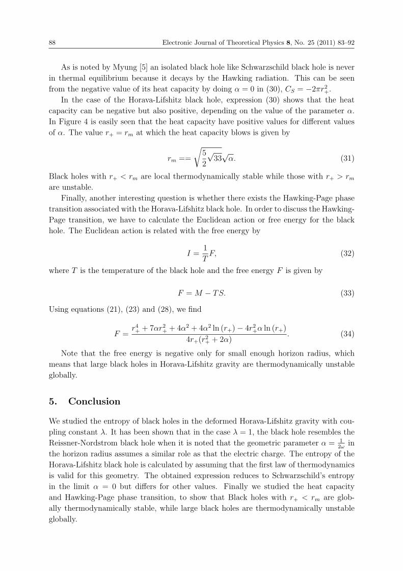
88 Electronic Journal of Theoretical Physics 8, No. 25 (2011) 83–92
As is noted by Myung [5] an isolated black hole like Schwarzschild black hole is never
in thermal equilibrium because it decays by the Hawking radiation. This can be seen
from the negative value of its heat capacity by doing α = 0 in (30), CS = −2πr2+.In the case of the Horava-Lifshitz black hole, expression (30) shows that the heat
capacity can be negative but also positive, depending on the value of the parameter α.
In Figure 4 is easily seen that the heat capacity have positive values for different values
of α. The value r+ = rm at which the heat capacity blows is given by
rm ==
√5
2
√33√α. (31)
Black holes with r+ < rm are local thermodynamically stable while those with r+ > rmare unstable.
Finally, another interesting question is whether there exists the Hawking-Page phase
transition associated with the Horava-Lifshitz black hole. In order to discuss the Hawking-
Page transition, we have to calculate the Euclidean action or free energy for the black
hole. The Euclidean action is related with the free energy by
I =1
TF, (32)
where T is the temperature of the black hole and the free energy F is given by
F =M − TS. (33)
Using equations (21), (23) and (28), we find
F =r4+ + 7αr2+ + 4α2 + 4α2 ln (r+)− 4r2+α ln (r+)
4r+(r2+ + 2α). (34)
Note that the free energy is negative only for small enough horizon radius, which
means that large black holes in Horava-Lifshitz gravity are thermodynamically unstable
globally.
5. Conclusion
We studied the entropy of black holes in the deformed Horava-Lifshitz gravity with cou-
pling constant λ. It has been shown that in the case λ = 1, the black hole resembles the
Reissner-Nordstrom black hole when it is noted that the geometric parameter α = 12ω
in
the horizon radius assumes a similar role as that the electric charge. The entropy of the
Horava-Lifshitz black hole is calculated by assuming that the first law of thermodynamics
is valid for this geometry. The obtained expression reduces to Schwarzschild’s entropy
in the limit α = 0 but differs for other values. Finally we studied the heat capacity
and Hawking-Page phase transition, to show that Black holes with r+ < rm are glob-
ally thermodynamically stable, while large black holes are thermodynamically unstable
globally.

Electronic Journal of Theoretical Physics 8, No. 25 (2011) 83–92 89
References
[1] P. Horava. arXiv:0901.3775[hep-th]
[2] T. Takahashi and J. Soda, arXiv:0904.0554 [hep-th]. G. Calcagni, arXiv:0904.0829.E. Kiritsis and G. Kofinas, arXiv:0904.1334 [hep-th]. S. Mukohyama, arXiv:0904.2190[hep-th]. R. Brandenberger, arXiv:0904.2835 [hep-th].
[3] H. Lu, J. Mei and C. N. Pope, arXiv:0904.1595 [hep-th].
[4] R. G. Cai, L. M. Cao and N. Ohta, arXiv:0904.3670 [hep-th]. arXiv:0905.0751 [hep-th]
[5] Y. Myung. arXiv:0905.0957 [hep-th]; Physics Letters B 684, Issues 2-3, Pages 158-161,(2010)

90 Electronic Journal of Theoretical Physics 8, No. 25 (2011) 83–92
Fig. 1 Entropy as a function of the radius of outer horizon with ω = 1 , i.e. α = 12 .
Fig. 2 Entropy as a function of the radius of outer horizon for different values of ω.

Electronic Journal of Theoretical Physics 8, No. 25 (2011) 83–92 91
Fig. 3 Zoom of Figure 2, Showing the entropy as a function of the radius of outer horizon fordifferent values of ω.
Fig. 4 Heat capacity as a function of the radius of outer horizon for different values of ω.


EJTP 8, No. 25 (2011) 93–108 Electronic Journal of Theoretical Physics
Canonical Relational Quantum Mechanics fromInformation Theory
Joakim Munkhammar∗
Studentstaden 23:230, 752 33, Uppsala, Sweden
Received 7 January 2011, Accepted 10 February 2011, Published 25 May 2011
Abstract: In this paper we construct a theory of quantum mechanics based on Shannon
information theory. We define a few principles regarding information-based frames of reference,
including explicitly the concept of information covariance, and show how an ensemble of all
possible physical states can be setup on the basis of the accessible information in the local
frame of reference. In the next step the Bayesian principle of maximum entropy is utilized in
order to constrain the dynamics. We then show, with the aid of Lisi’s universal action reservoir
approach, that the dynamics is equivalent to that of quantum mechanics. Thereby we show
that quantum mechanics emerges when classical physics is subject to incomplete information.
We also show that the proposed theory is relational and that it in fact is a path integral version
of Rovelli’s relational quantum mechanics. Furthermore we give a discussion on the relation
between the proposed theory and quantum mechanics, in particular the role of observation and
correspondence to classical physics is addressed. In addition to this we derive a general form
of entropy associated with the information covariance of the local reference frame. Finally we
give a discussion and some open problems.c© Electronic Journal of Theoretical Physics. All rights reserved.
Keywords: Quantum Mechanics; Relational Quantum Mechanics; Information Theory; Shannon
information theory
PACS (2010): 03.65.-w; 03.67.-a; 03.67.Bg; 03.65.Ta; 03.67.Mn
”Information is the resolution of uncertainty.”
- Claude Shannon
1. Introduction
Quantum mechanics constitutes a conceptual challenge as it defies many pivotal classical
concepts of physics. Despite this the theoretical and experimental success of quantum
∗ E-Mail: [email protected]

94 Electronic Journal of Theoretical Physics 8, No. 25 (2011) 93–108
mechanics is unparallel [15]. The intuitive construction of classical mechanics and the
perhaps counter-intuitive quantum mechanical formulation of reality has thus amounted
to a problem of interpretation of quantum mechanics. The list of interpretations of quan-
tum mechanics is long, but perhaps the most common interpretations are: Copenhagen
[2], consistent histories [7], many worlds [5] and relational [15]. Many of these approaches
share most central features of quantum mechanics, the difference is mainly the philo-
sophical context in which they are situated. The canonical problem in these approaches
is perhaps the counter-classic, and in many peoples views, counter-intuitive principle
that physics is fundamentally based on probability. The perhaps strongest opponent of
a probability-based theory of physics was Einstein who constructed several unsuccessful
thought experiments and theories in order to disprove the commonly accepted view of
quantum mechanics [4]. As a matter of fact all approaches to create a non-probabilistic
version of quantum mechanics have failed [3]. It has also been proven, via for example
Bell’s theorems, that the construction of such a deterministic or ”local hidden variable
theory” is impossible [3]. Thus one has no choice but to conclude that physics, inevitably,
has quantum properties.
1.0.1 Relational Quantum Mechanics
It was Einstein’s revised concepts of simultaneity and frame of reference that inspired
Rovelli to formulate a theory of mechanics as a relational theory; relational quantum
mechanics. In this seminal approach frames of reference were utilized and only relations
between systems had meaning. This setup gave interesting solutions to several quantum-
related conceptual problems such as the EPR-paradox [15]. It may be concluded that
Rovelli recast physics in the local frame of reference in such a way that the interactions
between systems amounted to the observed quantum phenomena. A particular facet of
Rovelli’s approach was that any physical system could be observed in different states by
different observers ”simultaneously”. This property can be interpreted as an extension
of the concept of simultaneity in special relativity [15]. The theory of relational quantum
mechanics was based on the hypothesis that quantum mechanics ultimately arose when
there was a lack of information of investigated systems.
1.0.2 Universal Action Reservoir
In a recent paper Lisi gave an interesting approach to quantum mechanics based on
information theory and entropy [12]. He showed that given a universal action reservoir
and a principle for maximizing entropy quantum mechanics could be obtained. In his
paper the origin of the universal action reservoir was postulated as a principle and was
given no deeper explanation. This was addressed in recent papers by Lee [10, 11] where
he suggested that it was related to information theory coupled to causal horizons.

Electronic Journal of Theoretical Physics 8, No. 25 (2011) 93–108 95
1.0.3 Relational Quantum Mechanics and the Universal Action Reservoir
In this paper we shall recast Rovelli’s relational approach to quantum mechanics on the
concept of information covariance and connect it to Lisi’s canonical information theoretic
approach. In the process of this we show that the universal action reservoir is an inevitable
consequence of incomplete information in physics. This theory is, in spirit of Rovelli’s
approach, a generalization of the special relativistic concept regarding frames of reference.
2. Physics with Information Covariance
2.1 Principles for Information-based Frames of Reference
Let us assume that we have a set of observations of certain physical quantities of a physical
system. This is the obtained information regarding the system. For all other events that
has not been observed we only know that something possible happened. If we knew with
certainty what happened then we as observers would be in a frame of reference based
on complete information regarding the explored system. However such a theory would
require some form of a conservation law which would require that a physical system has
a predetermined state when not observed. Let us instead consider the opposite: Assume
that no observation is made of the system, then information regarding that system is not
accessible and thus not inferable without more observations. It is then reasonable that
anything physically possible could have occurred when it was not observed. If one can
base the laws of physics on the premise of only what is known in the frame of reference,
in terms of information, regarding any physical system in connection with the observer
and her frame then one has attained a high from of generality in the formulation of the
laws of physics. This amounts to a seemingly tautological yet powerful principle:
If a system in physics is not observed it is in any physically possible state.
We shall call this principle the principle of physical ignorance. In one sense this
principle is intuitive and trivial: the unknown is not known. In another more intricate
sense it violates a number of basic principles of physics such as many of the laws of classical
physics. The law of inertia is one such principle for example; the inertia of a body does not
necessarily hold when we do not observe it. However one cannot assume that Newton’s
laws or any other classical laws hold in a system for which limited information is known.
For all we know regarding classical physics is that it holds in a certain classical limit. The
definition of ”known” here is what information has become accessible in ones frame of
reference obtained through interaction with another system. The laws of physics should
thus be formulated in such a way that they hold regardless of information content in the
local frame of reference; the formulation of the laws of physics should be invariant with
respect to the information content. This amounts to a principle for the formulation of
the laws of physics:
The laws of physics are defined on the basis of the information in the frame of reference.
This principle shall be call the principle of information covariance. It’s scope of gen-
erality is similar to the principle of general covariance, which is the natural generalization

96 Electronic Journal of Theoretical Physics 8, No. 25 (2011) 93–108
of the frames of reference used in special relativity. The principle of information covari-
ance suggests that the frame of reference is entirely based on information; thus any new
observations will alter the information content and thus re-constrain the dynamics of the
studied system ”projected” within the frame of reference. One should also keep in mind
that physics cannot, in a frame of incomplete information, ”project” any information
through physical interactions that is not inferable from the accessible information. This
creates a form of locality of physics: Physics only exists in every frame of reference. Thus
there exists no such thing as an objective observer. It should be noted here that there
exists a similar notion of frames of reference in traditional relational quantum mechanics
[15]. The dynamics is derived from a different set of principles and formal setup but
arrives at a similar conclusions [15].
2.2 Formal Setup
Let us assume that we have a set of observations An regarding physical quantities of a
system C from a frame of reference K. The available information regarding the system C
in K is given by the information in the observed physical quantities An and what can be
inferred from them, the rest of the properties of the system are by the principle of physical
ignorance unknown. Formally according to the principle of physical ignorance we may
conclude that the possible configurations of the explored physical system C in the frame
of referenceK has to form a set of all possible physical configurations under the constraint
of the set of observations An for the system. Consider a set of configuration parameters
for each possible physical configuration or path in configuration space path = q(t). The
set of configurations parameters is parameterized by one or more parameters t. Then for
each physical system we may associate an action S[path] = S[q(t)] defined on the basis
of the configuration space path q(t). The structure of the action is here assumed to be
something of a universal quantity of information inherent to every frame of reference, it
is the paths in the configuration space of objects that is unknown to every observer until
observed. The action of a system is defined classically as S =∫L(q, q)dt, where L(q, q)
is the Lagrangian for the system [17]. Traditionally with the aid of a variation principle
the expected action of a classical system is used to derive the dynamics of the system
[17]. In quantum mechanics a probabilistic setup is performed, ideally via a path integral
formulation. In our situation we shall instead look for all possible configurations under
condition of the observations An in accordance with the previously defined principle
of physical ignorance. The possible actions, based on the possible configurations, are
each associated with a probability of occurring, p[path] = p[q(t)]. The sum of these
probabilities need to satisfy the ubiquitous normalization criterion:
1 =∑paths
p[path] =
∫Dqp[q], (1)
Along with this we may conclude that any functional, or observable quantity Q, has
an expected value according to the expression [12]:

Electronic Journal of Theoretical Physics 8, No. 25 (2011) 93–108 97
〈Q〉 =∑paths
p[path]Q[path] =
∫Dqp[q]Q[q]. (2)
We have the expected action 〈S〉 according to [12]:
〈S〉 =∑paths
p[path]S[path] =
∫Dqp[q]S[q]. (3)
As a measure of the information content, or rather lack thereof, we can construct the
entropy of the system according to:
H = −∑paths
p[path] log p[path] = −∫Dqp[q] log p[q]. (4)
So far we have merely utilized information theoretic concepts, we shall deal with
its physical consequences further on in this paper. Although the probabilities for the
events in system C observed from reference system K are yet undefined we have a set of
possible configurations that could occur for a system and we have associated a probability
of occurrence with each based on the ensemble setup above. In order to deduce the
probability associated with each possible event we need some form of restriction on the
ensemble of possibilities. In a Bayesian theory of interference there is a maximization
principle regarding the entropy of a system called the Principle of maximum entropy [8]
which postulates the following:
Subject to known constraints, the probability distribution which best represents the
current state of knowledge is the one with largest entropy.
This principle is utilized in several fields of study, in particular thermodynamics where
it serves as the second fundamental law [8]. We shall assume that this principle holds and
we shall utilize it as a restriction on our framework. In [12] Lisi performed the following
derivation which is worth repeating here. By employing Lagrange multipliers, λ ∈ C and
α ∈ C, the entropy (4) is maximized by:
H ′ = −∫Dqp[q] log p[q] + λ
(1−
∫Dqp[q]
)+ α
(〈S〉 −
∫Dqp[q]S[q]
), (5)
which simplified becomes:
H ′ = λ+ α〈S〉 −∫Dq(p[q] log p[q] + λp[q] + αp[q]S[q]). (6)
If we perform variation on the probability distribution we get:
δH ′ = −∫Dq(δp[q])(log p[q] + 1 + λ+ αS[q]) (7)
which is extremized when δH ′ = 0 which corresponds to the probability distribution:
p[q] = e−1−λe−αS[q] =1
Ze−αS[q] (8)

98 Electronic Journal of Theoretical Physics 8, No. 25 (2011) 93–108
which is compatible with the knowledge constraints [12]. By varying the Lagrange
multipliers we enforce the two constraints, giving λ and α. Especially one gets: e−1−λ = 1Z
where Z is the partition function on the form:
Z =∑paths
e−αS[path] =∫Dqe−αS[q] (9)
and the parameter α is determined by solving:
〈S〉 =∫DqS[q]p[q] =
1
Z
∫DqS[q]e−αS[q] = − ∂
∂αlogZ. (10)
In order to fit the purpose Lisi concluded that the Lagrange multiplier value; α ≡1i�. Lisi concluded that this multiplier value was an intrinsic quantum variable directly
related to the average path action 〈S〉 of what he called the universal action reservoir.
In similarity with Lisi’s approach we shall also assume that the arbitrary scaling-part of
the constant α is in fact 1/�. Lisi also noted that Planck’s constant in α is analogous
to the thermodynamic temperature of a canonical ensemble, i� ↔ kBT ; being constant
reflects its universal nature - analogous to an isothermal canonical ensemble [12]. This
assumption along with (9) brings us to the following partition function:
Z =∑paths
eiS[path]
� =
∫Dqei
S[q]� . (11)
By inserting (11) into (2) we arrive at the following expectation value for any physical
quantity Q:
〈Q〉 =∑paths
p[path]Q[path] =
∫DqQ[q]p[q] =
1
Z
∫DqQ[q]ei
S[q]� , (12)
This suggests that a consequence of the incomplete information regarding the studied
system is that physics is inevitably based on a probabilistic framework. Conversely, had
physics not been probabilistic in the situation of incomplete information then information
of the system could be inferred. But a process of inferring results from existing limited
information does not provide more information regarding that system than the limited
information had already provided. That would have required, as we previously argued, an
additional principle of perfect information. Instead it is only interaction that can provide
new information. We may conclude that by the principle of information covariance
physics is local and based only on the available information in the local information-based
frame of reference. In turn this this creates an ensemble of possible states with a definite
and assigned expectation value for each physical quantity in the studied system according
to (12). This formalism, which might be called information covariant, is then directly
compatible with the general principle of relativity wherein All systems of reference are
equivalent with respect to the formulation of the fundamental laws of physics.
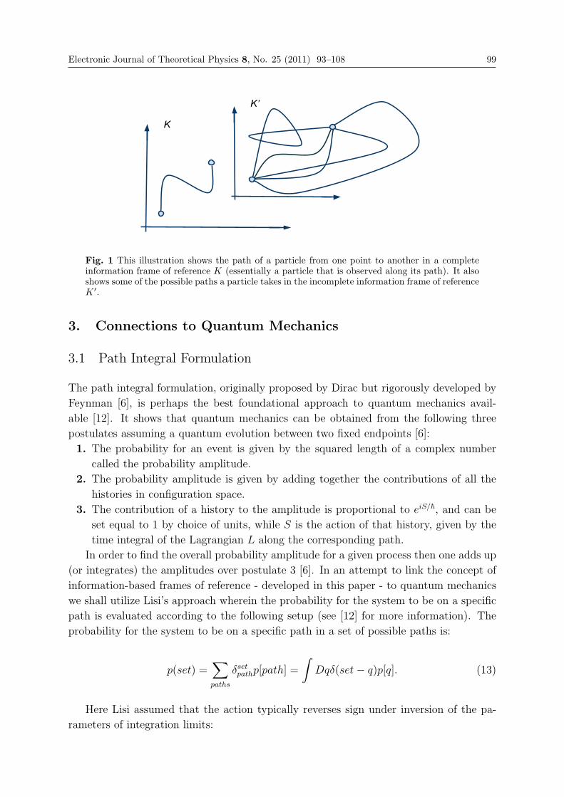
Electronic Journal of Theoretical Physics 8, No. 25 (2011) 93–108 99
Fig. 1 This illustration shows the path of a particle from one point to another in a completeinformation frame of reference K (essentially a particle that is observed along its path). It alsoshows some of the possible paths a particle takes in the incomplete information frame of referenceK ′.
3. Connections to Quantum Mechanics
3.1 Path Integral Formulation
The path integral formulation, originally proposed by Dirac but rigorously developed by
Feynman [6], is perhaps the best foundational approach to quantum mechanics avail-
able [12]. It shows that quantum mechanics can be obtained from the following three
postulates assuming a quantum evolution between two fixed endpoints [6]:
1. The probability for an event is given by the squared length of a complex number
called the probability amplitude.
2. The probability amplitude is given by adding together the contributions of all the
histories in configuration space.
3. The contribution of a history to the amplitude is proportional to eiS/�, and can be
set equal to 1 by choice of units, while S is the action of that history, given by the
time integral of the Lagrangian L along the corresponding path.
In order to find the overall probability amplitude for a given process then one adds up
(or integrates) the amplitudes over postulate 3 [6]. In an attempt to link the concept of
information-based frames of reference - developed in this paper - to quantum mechanics
we shall utilize Lisi’s approach wherein the probability for the system to be on a specific
path is evaluated according to the following setup (see [12] for more information). The
probability for the system to be on a specific path in a set of possible paths is:
p(set) =∑paths
δsetpathp[path] =
∫Dqδ(set− q)p[q]. (13)
Here Lisi assumed that the action typically reverses sign under inversion of the pa-
rameters of integration limits:

100 Electronic Journal of Theoretical Physics 8, No. 25 (2011) 93–108
St′ =
∫ t′
dtL(q, q) = −∫t′dtL(q, q) = −St′ . (14)
This implies that the probability for the system to pass through configuration q′ atparameter value t′ is:
p(q′, t′) =∫Dqδ(q(t′)− q)p[q] =
(∫ q(t′)=q′
Dqpt′[q]
)(∫q(t′)=q′
Dqpt′ [q]
)= ψ(q′, t′)ψ†(q′, t′),
(15)
in which we can identify the quantum wave function:
ψ =
∫ q(t′)=q′
Dqpt′[q] =
1√Z
∫ q(t′)=q′
Dqe−αSt′=
1√Z
∫ q(t′)=q′
DqeiSt′� . (16)
The quantum wave function ψ(q′, t) defined here is valid for paths t < t′ meeting at q′
while its complex conjugate ψ†(q′, t′) is the amplitude of paths with t > t′ leaving from q′.Multiplied together they bring the probability amplitudes that gives the probability of the
system passing through q′(t′), as is seen in (15). However, just as Lisi points out [12], thisquantum wave function in quantum mechanics is subordinate to the partition function
formulation since it only works when t′ is a physical parameter and the system is t′
symmetric, providing a real partition function Z. Indeed, the postulate of an information
covariant setup on the laws of physics according to the previous section suggests that
physics is ruled by the general complex partition function (9):
Z =∑paths
eiS[path]
� =
∫Dqei
S[q]� . (17)
How does this relate to the path integral formulation? The sum in the partition func-
tion (17) is a sum over paths. Let us take the common situation when the path is that
of a particle between two points. We can then conclude that each term is on the form
eiS[path]/� which is equivalent to postulate 3. Furthermore all paths are added, thus postu-
late 2 is also checked. Also, at least for the situation where p(q′, t′) = ψ(q′, t′)ψ†(q′, t′) thesum adds up to the probability density, checking postulate 1 as well. Thus we may con-
clude that the information covariant approach is equivalent to the canonical path integral
formulation of quantum mechanics under the circumstances provided for it.
3.2 Quantum Properties
The path integral formulation is canonical for quantum mechanics and covers the wide
variety of special features inherent to quantum mechanics [6, 12]. Since the approach in
this paper is equivalent to the path integral formulation in most aspects, some properties
are be worth discussing. A pivotal component of quantum mechanics is the canonical
commutation relation which gives rise to the Heisenberg uncertainty principle [3, 6]. For

Electronic Journal of Theoretical Physics 8, No. 25 (2011) 93–108 101
Fig. 2 This illustration shows on the left hand side the uncertainty of path of a particle fromone point to another and on the right hand side that the particle takes all possible paths fromone point to another. These two interpretations are equivalent under the general interpretationthat information is incomplete. Uncertainty in path means in practice that it takes any possiblepath until we observe it, a superposition of states is inevitable when information is incomplete.
example the famous commutation relation between position x and momentum p of a
particle is defined as:
[x, p] = i�. (18)
This can be obtained through the path integral formulation by assuming a random
walk of the particle from starting point to end point [6]. This works with this theory as
well under the same considerations since a random walk is equivalent to a walk with no
information about direction. In the path integral formulation it is also possible to show
that for a particle with classical non-relativistic action (where where m is mass and x is
position):
S =
∫mx2
2dt, (19)
that the partition function Z in the path integral formulation turns out to satisfy the
following equation [6]:
i�∂Z
∂t=[− 1
2∇2 + V (x)
]Z. (20)
This is the Schrodinger equation for Z = ψ and where V (x) is a potential [3]. It
is also possible to show the conservation of probability from the Schrodinger equation
(20) [3]. Here we can see that the traditional usage of operators on a Hilbert space in
quantum mechanics is a useful tool when information is incomplete. Another interesting
aspect of quantum mechanics is the superposition principle which states that a particle
occupies all possible quantum states simultaneously [3]. That the dynamics of a system
is fundamentally unknown or occupying all states simultaneously are both parts of the
same concept that information is incomplete regarding the system. The popular quantum
superposition thought experiment Schrodinger’s cat in which the alive/dead state of a
cat in a hazardous closed box is also evidently based on the lack of information regarding
the state of the cat. The superposition is intuitively equivalent to the lack of information.
The resolution of this problem in this theory is that the state of the cat is fundamentally

102 Electronic Journal of Theoretical Physics 8, No. 25 (2011) 93–108
unknown in our system of reference until we open the box and observe it, thus obtaining
information. The situation is also relational because even when information is obtained
the information is only inherent to our frame of reference which might not necessarily
be the same for any other frame of reference. For a complete verification that quantum
mechanics can be interpreted as a relational theory see [15]. The proof that quantum
mechanics can be interpreted as relational is constructed with Bra-kets in Hilbert spaces
and is directly related to a linearity inherent to quantum mechanics. Another interesting
topic worth mentioning here is the famous double slit experiment. The setup is as follows:
one has two slits and behind them a detection screen is setup. Some form of beam of
particles is then sent through the slits and a statistical pattern is shown on the detection
screen [3]. The result is an interference pattern equivalent to that described by the path
integral formulation of quantum mechanics. Such a pattern is not expected in classical
mechanics. The interpretation from the theory developed in this paper goes as follows:
due to the lack of information in the local information-based frame of reference a particle
takes any possible path, a similar interpretation was given by Lee [10]. This situation
is equivalent to the path integral formulation. The particle is, in our frame of reference,
wave-like until we observe it. This shows how the ubiquitous wave-particle dualism arises
under the lack of information. As far as observation goes, we will discuss that in section
3.5 below. Quantum entanglement is also a particular feature of quantum mechanics
that has spurred interpretational complications regarding quantum mechanics. Quantum
entanglement implies, among other things, that information can travel at a superluminal
speeds in most interpretations of quantum mechanics [4]. This violates the principle of
invariant speed of light inherent to special relativity [4]. However it has been solved
for relational quantum mechanics by postulating that physics is local, and then it can
be shown that no superluminal transfer of information occurs [11]. Since the theory
presented in this paper by design is relational the same conceptual solution holds. We will
discuss the connection between the theory developed in this paper and Rovelli’s version
of relational quantum mechanics in section 3.3 below. Since the theory developed in this
paper does not violate quantum mechanics it ought also to be completely compatible
with the Bohm-De Broglie pilot-wave approach [1] to quantum mechanics.
3.3 Connections to Relational Quantum Mechanics
Relational quantum mechanics is a theory of quantum mechanics based on the notion
that only systems in relation have meaning [15]. The observer and the partially observed
system makes out such a system typically. This addresses the problem of the third person
or Wigner’s friend as it is also called in which an observer observes another observer ob-
serving. The problem is solved by assuming that the two observers may ”simultaneously”
observe different states regarding the same object under observation. This is shown to be
a legal construction in quantum mechanics and is, as Rovelli points out, non-antagonistic
towards the most common formulations of quantum mechanics [15]. Furthermore, in his
seminal paper introducing relational quantum mechanics Rovelli postulates that quantum

Electronic Journal of Theoretical Physics 8, No. 25 (2011) 93–108 103
mechanics arises from the lack of information in classical physics. Given these facts one
might ask the following question: what is the similarity and what is the difference between
Rovelli’s approach and the theory developed in this paper? First of all our approach is
relational and based on a local frame of reference, which is similar to the concept used
by Rovelli. Second, this theory of quantum mechanics is based on information which is
similar to that used in Rovelli’s approach. There are two main differences. First of all this
theory is based on a few principles - different than those used by Rovelli - that sets the
foundation for a information covariant relational theory of physics. Second, it utilizes an
ensemble setup of Shannon information theory, developed by Lisi, which equips relational
quantum mechanics with an information-based path integral formulation.
3.4 Correspondence Principle
The correspondence from quantum mechanics, or any quantum field theory, to classical
physics is when � → 0 or more generally when S >> �. Since this theory is equivalent
to the canonical path integral approach to quantum mechanics under reasonable consid-
erations we may state tautologically that the correspondence to classical physics follows
the same limits as for regular quantum mechanics. The meaning of the correspondence is
also reasonable: If � descends to zero the partition function will ”collapse” and give only
one expected value for each quantity: The most expected one which by the Ehrenfest
theorem is the classical [3]. If the action is very large (S >> �) the situation is the
same; the larger the ratio between the classical action and Planck’s reduced constant is
the more likely the classical outcome is.
3.5 Observations and Wave Function Collapse
Observation is by definition obtaining information from a studied object [13, 12]. In order
to obtain information regarding a system one has to interact with it. This suggests that
observation of a system in practice is interacting with it, a view of observation that is
also held within the field of relational quantum mechanics [15]. In quantum mechanical
terms when an observation is performed then a wave function collapse occurs [3]. In the
theory developed in this paper the probability for a specific path (or state) becomes one.
Naturally the quantum expectation value for a quantity Q simply becomes the one for
the observed path A:
〈Q〉 =∑paths
p[path]Q[path] =
∫Dqp[q]Q[q] =
1
Z
∫DqQ[q]ei
S[q]� = Q[A]. (21)
Observation of a system limits the possibilities of that system by obtaining information
about it. The kinematics of a system, as viewed from our frame of reference, is based on
the local information about it by the principle of information covariance.

104 Electronic Journal of Theoretical Physics 8, No. 25 (2011) 93–108
4. Notes on Relativistic Invariance
The theory developed in this paper is by definition implicitly relativistic. The relativistic
kinematics inherent to special relativity should hold in this theory under at least the
same conditions for which the canonical path integral formulation is relativistic. In the
situation of complete information (or S >> �) the laws of (special) relativity hold in the
classical sense. We shall not detail the relativistic concepts further in this paper, nor
shall we attempt at constructing a general relativistic, or a general information covariant
theory of gravitation for the information-based frames of reference. Instead, this is left
for future investigation. However one might presume that such an approach might share
certain properties with the relational approach to quantum gravity [15].
5. Entropy
A great deal of this paper has consisted of meshing together mathematical structures
derived by previous authors under a new set of principles. In contrast to this we shall
here provide an explicit calculation of the entropy associated with an information-based
frame of reference. We defined the entropy as follows (4):
H = −∑paths
p[path] log p[path] = −∫Dqp[q] log p[q]. (22)
The entropy (22) is based purely on information theory and has thus no obvious direct
connection to physical quantities. Let us for this sake allow a scaling constant between
the information entropy H and the thermodynamical entropy H:
H ≡ kH. (23)
It was shown that after maximizing the entropy the probability of a specific path
becomes (8):
p[path] =1
Zei
S[path]� . (24)
Despite the fact that the probability (24) is a complex entity and thus ill-defined in
traditional probability theories it might still have meaning when used to calculate the
entropy. Insert (24) in (22):
H = −k∑paths
p[path]
(iS[path]
�− logZ
)(25)
We also have the normalization (1):
1 =∑paths
p[path], (26)
and the expression for the expected action (3):

Electronic Journal of Theoretical Physics 8, No. 25 (2011) 93–108 105
〈S〉 =∑paths
p[path]S[path] (27)
Together (25), (26), (27) and the fact that the partition function Z is path-independent
brings the following general expression for the entropy of the system:
H = −k( ∑
paths
p[path]iS[path]
�−
∑paths
p[path] logZ
)= −k
(i〈S〉�− logZ
). (28)
Let us now further assume the special case when the following identity holds:
ψ = Z. (29)
This identity holds at least when ψ = ψ(q′, t′) and t′ is a symmetric physical param-eter, just as described in section 3.1. Let us also assume that the structure of the wave
function is as follows:
ψ = ReiSc� (30)
where R = |ψ| and Sc is the classical action [3]. This brings the following expression:
logψ = log |ψ|+ iSc
�. (31)
Together (28) and (31) amounts to the following special case of the entropy:
H = −k(i〈S〉�− i
Sc
�− log |ψ|
). (32)
If we assume the equivalence between the classical action SC and the expected action
〈S〉, which is in accordance with the Ehrenfest theorem [3], then we get the following
expression for entropy:
H = k · log |ψ|. (33)
An expression similar to (33) was suggested as a basis for the holographic approach
to gravity [18] in a somewhat more speculative paper recently [13]. In that approach
the constant was suggested to be k = −2kB, where kB was Boltzmann’s constant. The
expression for entropy (33) is strikingly similar to Boltzmann’s formula for entropy in
thermodynamics:
H = kB · log(W ), (34)
where H is the entropy of an ideal gas for the number W of equiprobable microstates
[14]. The suggested entropy (33) and it’s more general version (28) are, up to a scalable
constant, measures of the lack of information in the information-based frame of reference.

106 Electronic Journal of Theoretical Physics 8, No. 25 (2011) 93–108
6. Discussion
This paper proposes a conceptual foundation for quantum mechanics based on informa-
tion brought on by the concept of information covariance. This approach supports the
notion that physics is largely based on information, a concept that among others Wheeler
strongly endorsed [19]. The suggested framework in this paper, building on Lisi’s universal
action reservoir and Rovelli’s relational quantum mechanics, gives an intuitive description
of physics; Physics in the quantum realm is a consequence of the incompleteness of infor-
mation in the local frame of reference. By setting up an information covariant foundation
in the local frame of reference by means of a maximization of Shannon entropy on the
possible paths of a system we managed to - by using Lisi’s theorem - establish a canonical
formulation of relational quantum mechanics. This implies that Lisi’s proposed universal
action reservoir is the inevitable result of the observer ignorance of a system. We also
explicitly calculated the entropy associated with any quantum mechanical system.
6.1 Open Problems
This theory primarily serves as a conceptual framework for quantum mechanics. How-
ever it also brings new concepts like for example the particular entropy (33) of a quantum
mechanical system. The role and the application of the new entropy is not yet fully inves-
tigated. It could, for example, perhaps be related to holographic theories of gravitation
[13, 18]. In addition to this the theory might give interesting effects in quantum statisti-
cal mechanics. Another open issue is how to construct a general relativistic approach to
this theory. Such a theory ought to arrive at some similar problems that many quantum
gravity theories have stumbled upon because this theory is merely a relational version of
the canonical path integral formulation of quantum mechanics.
6.2 Final Comments
When cast in a local frame of reference physics has only a limited amount of information
with which to function. When physics is fundamentally bound by a limited amount of
information probabilistic effects will occur. By maximizing entropy probabilistic effects
of quantum physics arise. The result of subjecting classical mechanics to incomplete
information is quantum mechanics.
Acknowledgments
This work would not have been possible without the inspiration and the valuable ideas
shared in the great works of G. Lisi, C. Rovelli and J-W. Lee. I would also like to thank
prof. Lee for a review of the paper and for giving valuable comments.
Electronic Journal of Theoretical Physics 8, No. 25 (2011) 93–108 107
References
[1] D. Bohm, Quantum Theory, New York: Prentice Hall. 1989 reprint, Dover (1951).
[2] N. Bohr, Quantum mechanics and physical reality, Nature 136 pp 65 (1935).
[3] B.H.Bransden, C.J.Joachain, Quantum Mechanics, Pearson Education Limited,Second ed. (2000).
[4] A. Einstein, B.Podolsky, N.Rosen, Can Quantum-Mechanical Description of PhysicalReality be Considered Complete?, Phys. Rev. D. 47 pp 777-780 (1935).
[5] H. Everett, Relative State Formulation of Quantum Mechanics, Rev. Mod. Phys. vol29, pp 454-462 (1957).
[6] R.P. Feynman, A.R. Hibbs, Quantum Mechanics and Path Integrals, New York,McGraw-Hill (1965).
[7] R.B. Griffiths, Consistent histories and the Interpretation of Quantum Mechanics, J.Stat. Phys. 36 (1984).
[8] E.T. Jaynes, Information Theory and Statistical Mechanics, Phys. Rev. 106: 620(1957).
[9] E.T. Jaynes, Information Theory and Statistical Mechanics II, Phys. Rev. 108: 171(1957).
[10] J-W. Lee, Quantum mechanics emerges from information theory applied to causalhorizons, Found. Phys. DOI 10.1007/s10701-010-9514-3 (2010) : arXiv:1005.2739v2.
[11] J-W. Lee, Physics from information, arXiv:1011.1657v1 [hep-th] (2010).
[12] G. Lisi, Quantum mechanics from a universal action reservoir,arXiv:physics/0605068v1 [physics.pop-ph] (2006).
[13] J.D.Munkhammar, Is Holographic Entropy and Gravity the result of QuantumMechanics?, arXiv:1003.1262 (2010).
[14] F. Rief, Fundamentals of statistical and thermal physics, McGraw-Hill (1985).
[15] C. Rovelli, Relational Quantum Mechanics, arXiv:quant-ph/9609002 (1997).
[16] C.E. Shannon, The Mathematical Theory of Communication, Univ. Illinois Press,(1949).
[17] J.B.Marion, S.T.Thornton, Classical Dynamics of Particles and Systems, Harcourt(1995).
[18] E.Verlinde, On the Origin of Gravity and the Laws of Newton, arXiv:1001.0785v1[hep-th] (2010).
[19] J.A.Wheeler, Information, physics, quantum: The search for links, W. Zurek (ed.)Complexity, Entropy, and the physics of information, Addison-Wesley (1990).


EJTP 8, No. 25 (2011) 109–126 Electronic Journal of Theoretical Physics
On the Logical Origins of Quantum MechanicsDemonstrated By Using Clifford Algebra: A Proofthat Quantum Interference Arises in a CliffordAlgebraic Formulation of Quantum Mechanics
Elio Conte∗
Department of Pharmacology and Human Physiology – TIRES – Center for InnovativeTechnologies for Signal Detection and Processing, University of Bari- Italy;
School of Advanced International Studies for Applied Theoretical and Non LinearMethodologies of Physics, Bari, Italy
Received 6 July 2010, Accepted 10 February 2011, Published 25 May 2011
Abstract: We review a rough scheme of quantum mechanics using the Clifford algebra.
Following the steps previously published in a paper by another author [31], we demonstrate
that quantum interference arises in a Clifford algebraic formulation of quantum mechanics. In
1932 J. von Neumann showed that projection operators and, in particular, quantum density
matrices can be interpreted as logical statements. In accord with a previously obtained result
by V. F Orlov , in this paper we invert von Neumann’s result. Instead of constructing logic
from quantum mechanics , we construct quantum mechanics from an extended classical logic. It
follows that the origins of the two most fundamental quantum phenomena , the indeterminism
and the interference of probabilities, lie not in the traditional physics by itself but in the logical
structure as realized here by the Clifford algebra.c© Electronic Journal of Theoretical Physics. All rights reserved.
Keywords: Quantum Mechanics; Quantum Interference; Clifford Algebra
PACS (2010): 03.65.-w; 42.50.-p; 03.65.Fd
1. Introduction
It is well known that in 1936 Birkhoff and von Neumann extended conventional quantum
mechanics by using quaternions in place of complex numbers in order to represent the
wave-functions and probability amplitudes in such a theory [1]. Starting with 1972 [2],
we began to apply Clifford algebra to a quantum mechanical framework, and our effort
culminated in 2000 [3], when we were able to reformulate the whole standard framework

110 Electronic Journal of Theoretical Physics 8, No. 25 (2011) 109–126
of quantum mechanics by a rough algebraic scheme, showing in detail that, by this rough
formulation, we may re-obtain all the standard quantum theory, and in particular we may
give proof of the existing quantization of systems, of basic features of harmonic oscillator,
of orbital angular momentum, of hydrogen atom, as well as of time evolution of quantum
systems, arriving to consider also the well known EPR problem of quantum mechanics
[4,5], the non locality, the Kochen and Specker theorem [5] as well as the more recent
Bell approach [7]. We covered all the standard features of quantum mechanics. Clifford
algebra gives an unifying framework of physical knowledge here including quantum me-
chanics, relativity, electromagnetism and other physical matter. When we introduce a
Clifford rough scheme of quantum mechanics, we cannot ignore the emerging salient fea-
ture of this formulation. It is that in this case we obtain a quantum mechanical theoretical
framework invoking only an algebraic structure that does not contain any further specific
requirement. This is a very important and salient feature of this algebraic structure.
Under a restricted and more methodological profile, it must be outlined with clearness
that such our approach to quantum mechanics does not give a formulation with alter-
native and entirely new ideas in quantum mechanics. In fact, recalling as example the
contributions given in [1], we outline that our elaboration results at least consistent with
old ideas that were known from the earliest days of quantum theory, although it contains
some, few, but very interesting new features that possibly deserve careful consideration.
In our effort there is, first of all, a research finality that is evident. There is also a didactic
finality. Starting with 2003 [8,910,11,12,13,16,17,20,26], we have performed a number of
experiments showing that the well known quantum interference effect may be observed
in perceptive-cognitive processes of human subjects, and, in particular, during their per-
ception and cognition of ambiguous figures. We will not enter here in the theoretical
and experimental details of such new obtained results [7], but their importance under the
perspective to establish if or not the psychological functions of human subjects involve
also the domain of quantum mechanics, results rather evident. In a recent contribution
we tested the possible Bell quantum violation in mental states, and we introduced for
the first time Clifford algebraic elements as basic quantum mental observables [17]. Such
new results in psychological and neurophysiological studies open interesting perspectives,
and lead as consequence that a whole set of researchers as psychologists and neurologists
could be interested to approach the whole scheme of quantum mechanics in order to fully
understand the possible potentialities of such theory when we attempt to explain by it
some basic features of our mind and of our human thinking. In brief, a rough approach to
quantum mechanics is required since it is well known that such researchers in some cases
may have not the necessary mathematical competence to approach the sophisticated and
standard formalism of the traditional quantum mechanics. In these cases, our simplified,
rough , Clifford scheme of quantum mechanics, without violating the requirements of the
scientific rigour that is required, but allowing at the same time some derogation under the
strict formal profile, enables as counterpart to acquire the basic conceptual foundations of
a theory, and thus to apply such new knowledge in the proper but distant sphere of com-
petence. This is the basic objective that the effort, given in [3], may substantially reach

Electronic Journal of Theoretical Physics 8, No. 25 (2011) 109–126 111
at the previously mentioned didactic profile. Clifford algebra uses few basic rules and al-
gebraic elements. Therefore, the advantage to use such so restricted algebraic framework
in a didactic perspective to acquire knowledge of the basic foundations of quantum me-
chanics, may be of importance for the researchers who unfortunately may have not direct
competence in the standard language of quantum mechanics that, as it is well known,
holds about the abstract field of Hilbert space and of acting linear operators. Of course,
the finality to introduce such alternative didactic patterns is not new here. We remember,
as example, the excellent book of T.F. Jordan [18], that reaches the same objective using
the simple matrix form, and that inspired so much our elaboration. In any manner, our
principal objective is to evidence the profound existing link between quantum mechan-
ics and Clifford algebra since this specific link opens some basic questions that are of
relevant and basic interest for the same widening of the basic foundations, nature and
meaning of quantum mechanics in the whole complex of unifying physical knowledge. It
offers also didactic opportunities. Therefore, our selected objective remains confined to
the analysis and examination of such existing link. To this purpose, it may be of interest
the result that we obtain in the present paper. We proof that quantum interference leads
necessarily to a Clifford algebraic formulation of quantum mechanics. Consequently, it
adds still rigour to the Clifford algebraic formulation of quantum mechanics .
2. A Clifford Algebraic Rough Scheme of Quantum Mechanics
Let us explain briefly the basic framework of our approach [3].
Let us give a proper definition of Clifford algebra. By using the Clifford algebra in our
rough quantum mechanical scheme it is intended that, specifically, a Clifford algebra is a
unital associative algebra which contains and is generated by a vector space V equipped
with a quadratic form Q. The Clifford algebra C�(V ,Q) is the algebra generated by V
subjected to the condition
v2 = Q(v) for all v ∈ Vwhere
uv + vu = 1/2(Q(u, v)−Q(u)−Q(v))
is the symmetric bilinear form associated to Q.
We will utilize and follow the work that, starting with 1981, was developed by Y.
Ilamed and N. Salingaros [19], using sometimes the same technique that these authors
introduced in their work.
Let us anticipate that only two basic assumptions, quoted as (a) and (b), are required
in order to formulate such rough scheme of quantum mechanics.
Let us consider three abstract basic elements, ei, with i = 1, 2, 3, and let us admit the
following two assumptions :
(1) it exists the scalar square for each basic element:
e1e1 = k1 , e2e2 = k2, e3e3 = k3 with ki ∈ � (1)
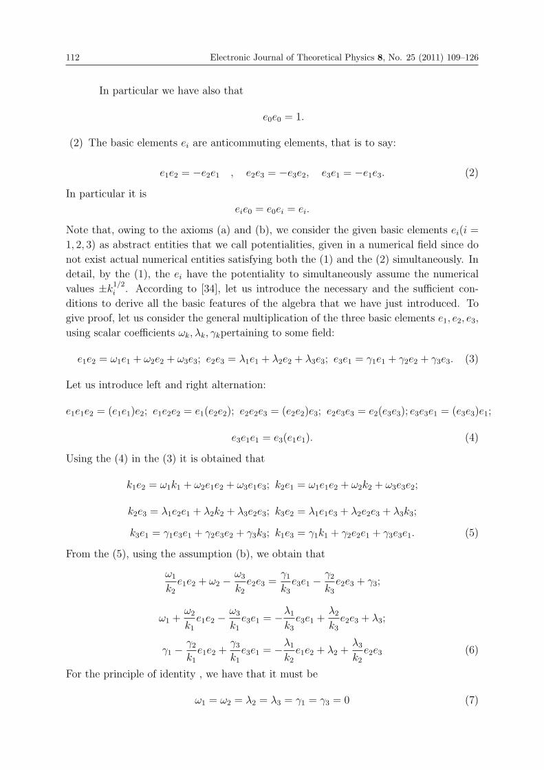
112 Electronic Journal of Theoretical Physics 8, No. 25 (2011) 109–126
In particular we have also that
e0e0 = 1.
(2) The basic elements ei are anticommuting elements, that is to say:
e1e2 = −e2e1 , e2e3 = −e3e2, e3e1 = −e1e3. (2)
In particular it is
eie0 = e0ei = ei.
Note that, owing to the axioms (a) and (b), we consider the given basic elements ei(i =
1, 2, 3) as abstract entities that we call potentialities, given in a numerical field since do
not exist actual numerical entities satisfying both the (1) and the (2) simultaneously. In
detail, by the (1), the ei have the potentiality to simultaneously assume the numerical
values ±k1/2i . According to [34], let us introduce the necessary and the sufficient con-
ditions to derive all the basic features of the algebra that we have just introduced. To
give proof, let us consider the general multiplication of the three basic elements e1, e2, e3,
using scalar coefficients ωk, λk, γkpertaining to some field:
e1e2 = ω1e1 + ω2e2 + ω3e3; e2e3 = λ1e1 + λ2e2 + λ3e3; e3e1 = γ1e1 + γ2e2 + γ3e3. (3)
Let us introduce left and right alternation:
e1e1e2 = (e1e1)e2; e1e2e2 = e1(e2e2); e2e2e3 = (e2e2)e3; e2e3e3 = e2(e3e3); e3e3e1 = (e3e3)e1;
e3e1e1 = e3(e1e1). (4)
Using the (4) in the (3) it is obtained that
k1e2 = ω1k1 + ω2e1e2 + ω3e1e3; k2e1 = ω1e1e2 + ω2k2 + ω3e3e2;
k2e3 = λ1e2e1 + λ2k2 + λ3e2e3; k3e2 = λ1e1e3 + λ2e2e3 + λ3k3;
k3e1 = γ1e3e1 + γ2e3e2 + γ3k3; k1e3 = γ1k1 + γ2e2e1 + γ3e3e1. (5)
From the (5), using the assumption (b), we obtain that
ω1
k2e1e2 + ω2 −
ω3
k2e2e3 =
γ1k3e3e1 −
γ2k3e2e3 + γ3;
ω1 +ω2
k1e1e2 −
ω3
k1e3e1 = −
λ1k3e3e1 +
λ2k3e2e3 + λ3;
γ1 −γ2k1e1e2 +
γ3k1e3e1 = −
λ1k2e1e2 + λ2 +
λ3k2e2e3 (6)
For the principle of identity , we have that it must be
ω1 = ω2 = λ2 = λ3 = γ1 = γ3 = 0 (7)

Electronic Journal of Theoretical Physics 8, No. 25 (2011) 109–126 113
and
−λ1k1 + γ2k2 = 0 γ2k2 − ω3k3 = 0 λ1k1 − ω3k3 = 0 (8)
The (8) is an homogeneous system admitting non trivial solutions since its determinant
Λ = 0, and the following set of solutions is given:
k1 = −γ2ω3, k2 = −λ1ω3, k3 = −λ1γ2. (9)
Admitting k1 = k2 = k3 = +1, it is obtained that
ω3 = λ1 = γ2 = i (10)
In this manner, using the (3), a theorem, showing the existence of such algebra, is proven.
The basic features of this algebra are given in the following manner
e1e2 = −e2e1 = ie3; e2e3 = −e3e2 = ie1; e3e1 = −e1e3 = ie2; i = e1e2e3 (11)
The content of this theorem is thus established: given three abstract basic elements
as defined in (a) and (b), an algebraic structure is established with four generators
(e0, e1, e2, e3).
Of course, as counterpart, the (11) are well known also in quantum mechanics and the
isomorphism with Pauli’s matrices at various orders is well known and discussed in detail
in [34]. Here, they have been derived only on the basis of two algebraic assumptions,
given respectively in (a) and (b).
We may now add some comments to the previous formulation.
Let us attempt to identify the phenomenological counterpart of the algebraic structure
given in (1), (2), and (11) with
e21 = 1, e22 = 1, e23 = 1 (12)
A generic member of our algebra is given by
x =3∑
i=0
xiei (13)
with xi pertaining to some field �or C. The (12) evidences that the ei are abstract
potential entities, having the potentiality that we may attribute them the numerical
values, or ±1. Admitting to be p1(+1)the probability to attribute the value (+1)to e1 andp1(−1) the probability to attribute (−1), considering the same corresponding notationfor the two remaining basic elements, we may introduce the following mean values:
< e1 >= (+1)p1(+1) + (−1)p1(−1), < e2 >= (+1)p2(+1) + (−1)p2(−1),
< e3 >= (+1)p3(+1) + (−1)p3(−1). (14)
Selected the generic element of the algebra, given in (13), its mean value results
< x >= x1 < e1 > +x2 < e2 > +x3 < e3 > (15)

114 Electronic Journal of Theoretical Physics 8, No. 25 (2011) 109–126
Let us call
a = x21 + x22 + x23 (16)
so that
−a ≤ x1 < e1 > +x2 < e2 > +x3 < e3 > ≤ a (17)
and
−1 ≤< ei > ≤ +1 i = (1, 2, 3) (18)
The (17) must hold for any real number xi, and, in particular, for
xi =< ei >
so that we have the fundamental relation
< e1 >2 + < e2 >
2 + < e3 >2≤ 1 (19)
See details of this proof in ref. [32] for quantum mechanics in simple matrix form and for
its extension in Clifford algebra in ref. [3]
Let us observe some important things:
(1) The (19), owing to the (14), says that probabilities for basic elements ei are not
independent and this is of basic importance to acknowledge the essential features of
a rough quantum mechanical scheme.
(2) The (19) still says that also mean values of ei are not independent. In detail, the
(19) may be considered to represent a general principle of ontic potentialities. We
have here a formulation of a basic, irreducible, ontic randomness. In particular, it
affirms that we never can attribute simultaneously, definite numerical values to two
basic elements ei. Let us consider, as example, < e3 >= +1, that is to say that
e3 → +1, we have consequently that < e1 >=< e2 >= 0, that is to say that e1 and
e2 are both in a complete condition of randomness. The values are equally probable,
there is full indetermination. We have a condition of ontic potentiality.
In conclusion, by using only the axioms (a) and (b), by the (11), the (14) and the (19),
we have delineated a rough scheme of quantum theory using only an algebraic structure.
Let us observe that the elective role in our formulation is performed in particular from the
axiom (b) that relates non commutativity of the basic elements. In this algebraic scheme
some principles of the basic quantum theoretical framework result to be represented. In
particular, this algebraic structure reflects the intrinsic indetermination and the ontic po-
tentiality that are basic components of quantum mechanics. This means that, in absence
of a direct numerical attribution, such basic elements are abstract entities that act hav-
ing an intrinsic, irreducible, indetermination, an ontic randomness, an ontic potentiality.
Therefore, by using such rough quantum mechanical scheme, we may explore what is the
actual role of potentiality in nature, what is its manner to combine with actual elements
of our reality and what is the manner in which potentiality may contribute to the general
dynamics of systems in Nature.
Let us add still some other feature of the scheme that we have in consideration. Let
us consider two generic elements of our algebra, given as in the (13), and let us indicate

Electronic Journal of Theoretical Physics 8, No. 25 (2011) 109–126 115
them by x and y. Owing to the (11), they will result in general not commutative, that is
to say
xy �= yx (20)
However, under suitable conditions, non-commutativity may fail and such abstract en-
tities return to have the actual and traditional numerical role in some selected field. In
this condition we have that xy = yx
Starting with 1974, [2] we introduced a theorem showing that necessary and sufficient
condition for two given algebraic elements, x and y, to be commutative is that
xy = yx↔ xj = λ yj , ∀λ(j = 1, 2, 3) (21)
This theorem regulates the passage from potentiality of abstract elements in this algebra
to actual numerical values relating instead any numerical field of our direct experience. In
quantum mechanics this passage from potentiality to actualisation is called the collapse
of wave function. An important feature of the theorem given in (21) is that the algebraic
structure given in (1), (2), (11), and (19) admits idempotents. Let us consider two of
such idempotents:
ψ1 =1 + e32
and ψ2 =1− e32
(22)
It is easy to verify that ψ21 = ψ1 and ψ
22 = ψ2. Let us examine now the following algebraic
relations:
e3ψ1 = ψ1e3 = ψ1 (23)
e3ψ2 = ψ2e3 = −ψ2 (24)
Similar relations hold in the case of e1or e2. The relevant result is that the (23) establishes
that the given algebraic structure, with reference to the idempotent ψ1, attributes to
e3 the numerical value of +1while the (24) establishes that, with reference toψ2, the
numerical value of -1 is attributed to e3.
The conclusion is very important: the conceptual counter part of the (23) and (24) is
that we are in presence of a self-referential process. On the basis of such self-referential
process, as given in (23) and in (24), this algebraic structure is able to attribute a precise
numerical value to its basic elements. Each of the three basic elements may “ transitate”
from the condition of pure potentiality to a condition of actualization, that is to say,
in mathematical terms, from the pure, symbolic representation of their being abstract
elements to that one of a real number. Let us remember that, on the basis of the (19),
this self-referential process may regard each time one and only one of the three basic
elements. It is well known that self-referential processes relate the basic phenomenology
of our mind and consciousness.
In conclusion, for the first time we have an algebraic structure that represents a rough
quantum mechanical scheme and that, at the same time, evidences, on the basis of a self-
referential process, that it is possible a transition from potentiality to actualization. Other
features of our formulation are given in [2,3,11]. It remains to evidence that a profound
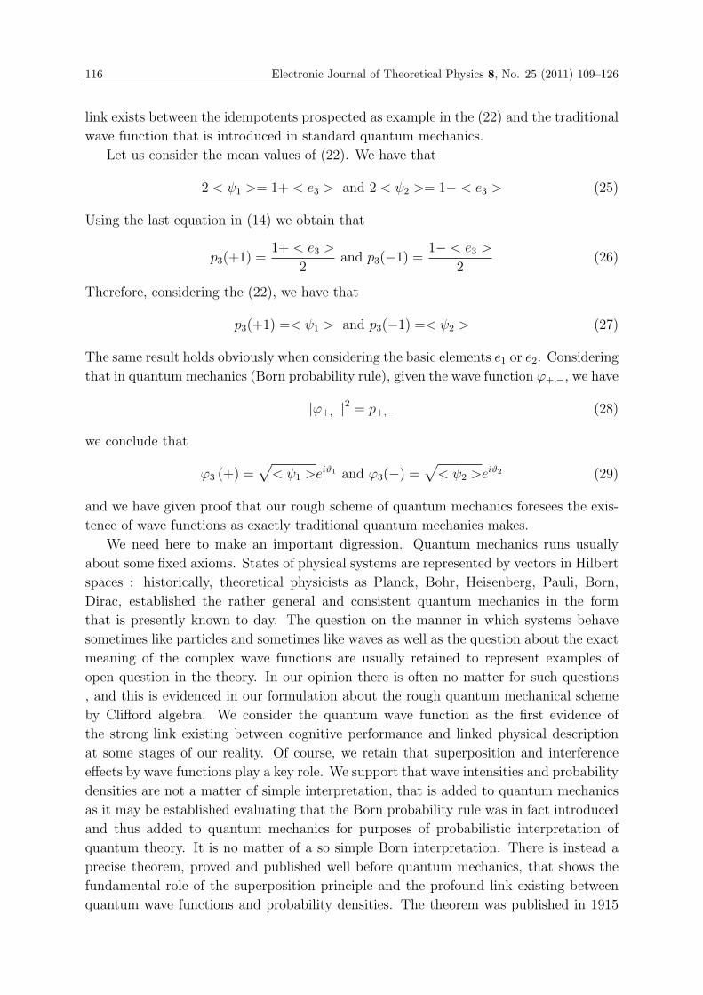
116 Electronic Journal of Theoretical Physics 8, No. 25 (2011) 109–126
link exists between the idempotents prospected as example in the (22) and the traditional
wave function that is introduced in standard quantum mechanics.
Let us consider the mean values of (22). We have that
2 < ψ1 >= 1+ < e3 > and 2 < ψ2 >= 1− < e3 > (25)
Using the last equation in (14) we obtain that
p3(+1) =1+ < e3 >
2and p3(−1) =
1− < e3 >
2(26)
Therefore, considering the (22), we have that
p3(+1) =< ψ1 > and p3(−1) =< ψ2 > (27)
The same result holds obviously when considering the basic elements e1 or e2. Considering
that in quantum mechanics (Born probability rule), given the wave function ϕ+,−, we have
|ϕ+,−|2 = p+,− (28)
we conclude that
ϕ3 (+) =√< ψ1 >e
iϑ1 and ϕ3(−) =√< ψ2 >e
iϑ2 (29)
and we have given proof that our rough scheme of quantum mechanics foresees the exis-
tence of wave functions as exactly traditional quantum mechanics makes.
We need here to make an important digression. Quantum mechanics runs usually
about some fixed axioms. States of physical systems are represented by vectors in Hilbert
spaces : historically, theoretical physicists as Planck, Bohr, Heisenberg, Pauli, Born,
Dirac, established the rather general and consistent quantum mechanics in the form
that is presently known to day. The question on the manner in which systems behave
sometimes like particles and sometimes like waves as well as the question about the exact
meaning of the complex wave functions are usually retained to represent examples of
open question in the theory. In our opinion there is often no matter for such questions
, and this is evidenced in our formulation about the rough quantum mechanical scheme
by Clifford algebra. We consider the quantum wave function as the first evidence of
the strong link existing between cognitive performance and linked physical description
at some stages of our reality. Of course, we retain that superposition and interference
effects by wave functions play a key role. We support that wave intensities and probability
densities are not a matter of simple interpretation, that is added to quantum mechanics
as it may be established evaluating that the Born probability rule was in fact introduced
and thus added to quantum mechanics for purposes of probabilistic interpretation of
quantum theory. It is no matter of a so simple Born interpretation. There is instead a
precise theorem, proved and published well before quantum mechanics, that shows the
fundamental role of the superposition principle and the profound link existing between
quantum wave functions and probability densities. The theorem was published in 1915
Electronic Journal of Theoretical Physics 8, No. 25 (2011) 109–126 117
by Fejer and by Riesz [21,22]. There is an excellent paper by F.H. Frohner that, time ago,
properly evidenced the profound existing link between probability theory and quantum
mechanics [23]. For any purpose, we retain of importance to report here this theorem
that states
0 ≤ ρ(x) ≡n∑
l=−ncle
ilx ≡∣∣∣∣∣
n∑k=0
akeikx
∣∣∣∣∣2
≡ |ψ(x)|2
where the complex Fourier polynomial ψ(x) has not restrictions, where instead to the
Fourier polynomial ρ(x) is imposed the requirement of its reality and non-negativity.
So, in conclusion, such required link exists and it is mathematically established. This
is the matter in spite of the continuous claims that in quantum mechanics such link holds
only on the basis of a given Born’s interpretation.
Let us look now to another link existing between standard quantum mechanics and our
rough quantum mechanical scheme. It is well known the central role that is developed in
traditional quantum mechanics from density matrix operator . In our scheme of quantum
mechanics, we have the corresponding algebraic member that is given in the following
manner
ρ = a+ be1 + ce2 + de3 (30)
with
a =|c1|2
2
+|c2|2
2
, b =c∗1c2 + c1c
∗2
2, c =
i(c1c∗2 − c∗1c2)2
, d =|c1|2 − |c2|2
2(31)
where in matrix notation, e1,e2, ande3 are the well known Pauli matrices. The complex
coefficients
ci(i = 1, 2)are the well known probability amplitudes for the considered quantum
state
ψ =
⎛⎜⎝ c1
c2
⎞⎟⎠ and |c1|2 + |c2|2 = 1 (32)
For a pure state in quantum mechanics it is ρ2 = ρ. In our scheme a theorem may be
demonstrated that
ρ2 = ρ↔ a =1
2and a2 = b2 + c2 + d2 (33)
The details of this our theorem are given in [24,25]. Written in matrix form we have also
Tr(ρ) = 2a = 1. In this manner we have the necessary and sufficient conditions for ρ to
represent a potential state or, in traditional quantum mechanics, to have a superposition
of states.
We have to examine now quantum time evolution.
It is clear that the quantum like scheme we are discussing is based on the two dimen-
sional abelian subalgebra of the four dimensional Clifford algebra. Of course, generally
speaking, we are considering our quantum rough scheme using quantum like operators
acting on vectors of a given Hilbert space.

118 Electronic Journal of Theoretical Physics 8, No. 25 (2011) 109–126
For time evolution, we consider Heisenberg description. Given the operator α con-
nected to some observable A, the mean value at a given time t will be given as
< αt >= (ψ0, U−1αUψ0)
with U time evolution operator.
It is well known that we have
ihd < α >
dt= ih <
∂α
∂t+
1
ih[α,H] > (34)
anddα
dt=∂α
∂t+
1
ih[α,H] (35)
where His the Hamiltonian of the system. The manner in which such Hamiltonian may
be constructed for psychological states in the Clifford algebra framework is given in [8].
It is well known that members of Clifford algebra transform according to
e′i = U+eiU, U+U = 1 (36)
In [3] we give a rigorous proof of the (34) and the (35) using the Clifford algebra.
Still we have to remember here that in the past there were attempts to go beyond the
linear Schrodinger equation [14,15,27,28,29,30], but, as well as we know, nobody tried to
do the same thing in the Heisenberg’s picture. It is very important to outline here that
in the non linear case, such two, Heisenberg and Schrodinger, representations, no more
result to be equivalent.
We have in fact that
U = exp(−ihHt) = 1− i
hHt+ (
iH
h)2t2
2!− (
iH
h)3t3
3!+ ........................ (37)
anddU
dt= − iH
h
[1− i
hHt+ (
iH
h)2t2
2!+ ...........
](38)
By using the Clifford rough scheme of quantum mechanics we are in the condition to take
account also for such possible non linear processes in Heisenberg like quantum represen-
tation.
3. Proof that Quantum Interference Arises in a Clifford Al-
gebraic Formulation of Quantum Mechanics and the Irre-
ducible, Ontic Randomness of Basic Clifford Algebraic Ele-
ments
Consider a beam of particles impinging on a beam splitter A so that randomly may be
either reflected to proceed a path L1 or transmitted to proceed along the path L2(Fig.1).
At the end of L1, the particles impinge on the upper side of a second beam splitter ,

Electronic Journal of Theoretical Physics 8, No. 25 (2011) 109–126 119
B, and it may be either reflected and detected by the detector D1 or transmitted and
detected by the detector D2.The particles arriving from path L2, impinge on the opposite
side of to be either transmitted reaching the detector D1 or reflected to reach the counter
D2. As it is well known we are considering here the interference pattern of a beam of
particles passing through a Mach Zender interferometer.
The considered random variable A assumes the value a = +1in the case of reflection
and the value a = −1 in the case of transmission. The random variable Bassumes the
value b = +1in the case of reflection and the value b = −1 in the case of transmission.We have a third variable C = ABthat is determined by the product of the values of A
and B.
In analogy with the rough quantum scheme previously developed we call still write
the mean value of A by < A > and
< A >= (a = +1)pab + (a = −1)pab (39)
the mean value of Bby < B > and
< B >= (b = +1)pab + (b = −1)pab (40)
and the mean value of C by < C > and
< C >= (ab; a = +1, b = +1)pab + (ab; a = +1, b = −1)pab+(ab; a = −1, b = +1)pab + (ab; a = −1, b = −1)pab (41)
Let us follow directly the argument as it was recently developed in [31]. According to
this interesting paper , we may write easily the expression of the probability for the
corresponding four alternatives (a = ±1, b = ±1) in the following manner
pab =1
4(1 + ax+ by + abz) (42)

120 Electronic Journal of Theoretical Physics 8, No. 25 (2011) 109–126
where
x ≡< A >, y ≡< B >, z ≡< C > . (43)
Still according to ref. [31] let us calculate the probability for counting the detector D1.
We have that
p++ =1
4(1 + x+ y + z) and p−− =
1
4(1− x− y + z) (44)
so that in the detector D1 we have
pD1 = p++ + p−− =1
2(1 + z) =
1
2(1+ < C >) (45)
In the case of the detector D2, we have
p+− =1
4(1 + x− y − z) and p−+ =
1
4(1− x+ y − z) (46)
and
pD2 = p+− + p−+ =1
2(1− z) =
1
2(1− < C >) (47)
This is of course the classical statistical argument holding on an epistemic interpretation
of randomness . In order to introduce the quantum like elaboration the author in ref.[31]
correctly introduced three new variables:
U = αA+ β B + γ C with α2 + β2 + γ2 = 1; (48)
V = λA+ μB + ν C , with λ2 + μ2 + ν2 = 1, αλ+ βμ+ γν = 0 (49)
and
W = δ A+ ωB + ϑC with δ = βν − γμ;ω = γλ− αν, ϑ = αμ− βλ, (50)
and considered
< U >= u (51)
plus
< V >=< W >= 0 (52)
in order to take into account a complete indetermination in the case of variables V and
W .
Following this argument one obtains
α < A > +β < B > +γ < C >= u ; (53)
λ < A > +μ < B > +ν < C >= 0;
δ < A > +ω < B > +ϑ < C >= 0
that admits solutions
< A >= αu , < B >= β u, < C >= γ u. (54)

Electronic Journal of Theoretical Physics 8, No. 25 (2011) 109–126 121
Inserting the (54) in the (42), one obtains
pab =1
4[1 + (α a+ β b+ γ ab)u] (55)
and
pD1 = p++ + p−− =1
2(1 + γ u) (56)
and
pD2 = p+− + p−+ =1
2(1− γ u) (57)
Let us comment the obtained results.
First consider the classical case.
Probability given in (42) must be between the well known limits
0 ≤ pab ≤ 1 (58)
Consequently, still according to the findings in ref.[31], < A >,< B >,< C >, are the
coordinates of a point inside the equilateral octahedron having the vertices
< A >= ±1, < B >= 0, < C >= 0; < B >= ±1, < A >= 0, < C >= 0;
< C >= ±1, < A >= 0, < C >= 0
The author in ref. [31] correctly argues that the first limiting values correspond to the case
of pure reflection (transmission) by A and equally probable reflection and transmission
by B and zero correlation. The second limiting values correspond to equally probable
reflection and transmission by A followed by pure reflection by B and zero correlation,
and the third limiting values correspond to the case of complete correlation between
the two splitters with equally probable transmission and reflection by A and B. These
are the limiting cases while for the other possible conditions we have average values of
the considered random variables having values less than one. This means that always
particles with both the values (±1) are present. We have that
−1 ≤< A > + < B > + < C >≤ +1 (59)
According to the (54) in the case of the (48)-(50) and (51)-(52) , we have that
−1 ≤ (α + β + γ) u ≤ +1 (60)
which implies that the absolute value of uis always smaller than one. Particles with both
values (±1) of A,B,C are always present, [31].
We may now explore the quantum case. Instead of the (45) and the (47) , of the (56)
and the (57) , the correct probabilities in quantum theory result to be
pD1 = p++ + p−− =1
2(1 + γ ) (61)
and
pD2 = p+− + p−+ =1
2(1− γ ) (62)

122 Electronic Journal of Theoretical Physics 8, No. 25 (2011) 109–126
that result to be
pD1 = p++ + p−− =1
2(1 + cosφ ) (63)
and
pD2 = p+− + p−+ =1
2(1− cosφ ) (64)
This is to say that we must have u = 1(u = −1), and
< A >= α, < B >= β, < C >= γ (65)
with
< A >2 + < B >2 + < C >2= 1 (66)
and
γ = cosφ
as polar angle of the unit vector on the sphere given in (66). This is to say that it must
be
< U2 >= 1 (67)
and
< V >=< W >= 0 (68)
to assure complete indetermination.
Let us consider again the variable U as given in the (48). It results that
U2 = (αA+ β B + γ C)(αA+ β B + γ C)
= α2 + β2 + γ2 + αβ(AB +BA) + αγ(AC + CA) + βγ(BC + CB)
= 1 + αβ(AB + BA) + αγ(AC + CA) + βγ(BC + CB). (69)
It is
< U2 >= 1+ < αβ(AB + BA) + αγ(AC + CA) + βγ(BC + CB) > . (70)
The only way to obtain the (67) is that
AB = −BA , AC = −CA, BC = −CB (71)
and this is to say that the variables A,B,C must be the basic elements of the Clifford
algebra, the ei(i = 1, 2, 3) basic elements that we introduced in the previous section in
the (1),(2),(11).
It is
A ≡ e1 , B ≡ e2, AB ≡ e1 e2 = ie3 (72)
Therefore, A,B,C, as given in the (48),(49), and the (50) are members of the Clifford
algebra.
So we reach the following conclusion.
Quantum mechanics holds about the basic phenomenon of quantum interference. We
may realize it using the basic elements, and the structure of the Clifford algebra. The

Electronic Journal of Theoretical Physics 8, No. 25 (2011) 109–126 123
author in [31] concluded that typical objects of the required kind are Hermitean matrices
with eigenvalues (±1).We may now take a step on.
Rather recently [32] we gave proof of two theorems on existing two Clifford algebras,
the A(Si) that has isomorphism with that one of Pauli matrices, and the Ni,±1 whereNi stands for the dihedral Clifford algebra. The salient feature was that by using such
two theorems, we showed that the Ni,±1 algebra may be obtained from the A(Si) algebra
when we attribute a numerical value (+1 or –1) to one of the basic elements (e1, e2, e3) of
the A(Si). The arising physical model was that the A(Si)−Clifford algebra refers to therepresentation of the general situation in quantum mechanics where the observer has no
right to decide on the state of a two-state system while instead, through the operation
represented by Ni,±1 algebra, he finally specifies which state is the one that will be or
is being observed. The A(Si)− algebra has as counterpart the description of quantum
systems that in standard quantum mechanics are considered in absence of observation
and quantum measurement while the Ni,±1 attend when a quantum measurement is
performed on such system with advent of wave function collapse. There is another salient
feature that needs to be outlined here. As said, under a Clifford algebraic profile, the
quantum measurement with wave function collapse induces the passage in the considered
quantum system from the A(Si) to Ni,+1or to the Ni,−1 algebras: it is of interest froma mathematical and physical view points to observe that in the passage from A(Si) to
N1,±1, each N1,±1 algebra has now its proper rules of commutation that are new and
different respect to standard ones calculated in A(Si). Under the profile of a quantum
measurement, wave function collapse is thus characterized, at least from an algebraic
view point, just from such transition from standard to new commutation rules for the
basic algebraic elements. This is an important feature that deserves careful physical
consideration.
In [32] we re-examined also the well known von Neumann postulate on quantum
measurement, and we gave a proper justification of such postulate by using such two
theorems. In detail, we studied some application of the above mentioned theorems to
some cases of interest in standard quantum mechanics, analyzing in particular a two
state quantum system, the case of time dependent interaction of such system with a
measuring apparatus and finally the case of a quantum system plus measuring apparatus
developed at the order n=4 of the considered Clifford algebras and of the corresponding
density matrix in standard quantum mechanics. In each of such cases, we found that
the passage from the algebra A(Si) to Ni,±1 actually describes the collapse of the wavefunction. We concluded that the actual quantum measurement has as counterpart in the
Clifford algebraic description, the passage from the A(Si) to the Ni,±1, reaching in thismanner the objective to reformulate von Neumann postulate on quantum measurement
and proposing at the same time a self-consistent formulation of quantum theory.
The aim of the present paper has been to propose a step on.
As it is well known, quantum mechanics runs about two basic foundations that are
the indeterminism and the quantum interference. It is also well known that in 1932 J.
124 Electronic Journal of Theoretical Physics 8, No. 25 (2011) 109–126
von Neumann [34] gave proof that the projection operators and, in particular, quantum
density matrices represent logical statements. We may say that he constructed a matrix
logic on the basis of quantum mechanics. In the present paper we have re-constructed
the two basic foundations of quantum mechanics starting from logic and thus arriving
to explain that quantum mechanics has logical origins. Not logic deriving from quantum
mechanics as in von Neumann but quantum mechanics having logical origins. This is
to say that the two basic foundations of quantum mechanics, the indeterminism and the
quantum interference, may be explained on a purely logical basis. In the development
of the paper we have used our Clifford rough scheme of quantum mechanics including
the theorems shown in [32]. No element of physics has been evoked by us but only
the idempotents of Clifford algebra , given in the (22) once again one has admitted the
necessary existence of the Clifford basic elements given in the (72). Such idempotents
represent of course in quantum mechanics the projection operators that were introduced
by von Neumann as logical statements. Therefore , a conclusion seems to be unavoidable.
We have to consider the basic foundations of quantum mechanics as basic framework
representing conceptual entities [33].
Acknowledgment
The author is indebted with the friend and colleague Alessandro Giuliani (Istituto Su-
periore di Sanita – Rome) for the continuous and stimulating discussions held during
the elaboration of the present paper about the fundamental theme on the possibility to
represent cognitive processes of mind by the classical and quantum profiles of the physics.
References
[1] Birkhoff, G., and von Neumann J., The logic of quantum mechanics, Ann. of Math.,37, 823 (1936)
[2] Conte E., New aspects of Indeterminism in Nature: quaternion quantum mechanics,Balkanski Matematicki Kongres, 24-30.6.1974
[3] Conte E., Biquaternion quantum mechanics, Pitagora Editrice, Bologna, 2000
[4] Conte E., The solution of the E.P.R. paradox in quantum mechanics, ProceedingsCongress-2002 on Fundamental problems of natural sciences and engineering, RussianAcademy of Sciences, 271-304, Saint-Petersburg, 2002
[5] Conte E., A Quantum Like Interpretation and Solution of Einstein, Podolsky, andRosen Paradox in Quantum Mechanics, arXiv:0711.2260
[6] Conte E., A Proof Of Kochen - Specker Theorem of Quantum Mechanics Using aQuantum Like Algebraic Formulation arXiv:0712.2992 .
[7] Bell J.S., Speakable and unspeakable in quantum mechanics, Cambridge UniversityPress, 1987

Electronic Journal of Theoretical Physics 8, No. 25 (2011) 109–126 125
[8] Conte, E., Todarello, O., Federici, A., Vitiello F., Lopane M., Khrennikov A., ZbilutJ.P., Some remarks on an experiment suggesting quantum-like behavior of cognitiveentities and formulation of an abstract quantum mechanical formalism to describecognitive entity and its dynamics. Chaos, Solitons and Fractals 31 (2007) 1076-1088
[9] Conte E., Pierri GP, Federici A., Mendolicchio L., Zbilut J.P., A model of biologicalneuron with terminal chaos and quantum like features, Chaos, Solitons and Fractals,30,774-780,2006
[10] Conte E., Khrennikov A., Todarello O., Federici A., Zbilut J. P.. Mental StatesFollow Quantum Mechanics during Perception and Cognition of Ambiguous Figures.Open Systems & Information Dynamics, (2009),Vol.16, No.1,1-17; available on linePhilPapers
[11] Conte E., Khrennikov Yuri, Todarello Orlando, Federici Antonio, Zbilut Joseph P:On the Existence of Quantum Wave Function and Quantum Interference Effects inMental States: An Experimental Confirmation during Perception and Cognition inHumans. NeuroQuantology, (2009), First issue 2009 - available on line.
[12] Conte E.: Exploration of Biological Function by Quantum Mechanics. Proceedings10th International Congress on Cybernetics, 1983;16-23, Namur-Belgique.
[13] Conte E.: Testing Quantum Consciousness. NeuroQuantology (2008); 6 (2): 126-139.
[14] Khrennikov A.: Quantum-like brain: Interference of minds. BioSystems 84, 225-241(2006).
[15] Khrennikov A.: Information Dynamics in Cognitive, Psychological and AnomalousPhenomena. ser. Fundamental Theories of Physics, Kluwer Academic, 2004.
[16] Conte E., Todarello O., Federici A., Zbilut Joseph P.: Mind States followQuantum Mechanics during Perception and Cognition of Ambiguous Figures: a FinalExperimental Confirmation. arXiv:0802.1835
[17] Conte E., Khrennikov A., Todarello O., Federici A., Zbilut J. P.: A PreliminaryExperimental Verification On the Possibility of Bell Inequality Violation in MentalStates. NeuroQuantology, (2008); 6 (3): 214-221.
[18] Jordan T.F.,Quantum mechanics in simple matrix form, John Wiley and Sons, NewYork, 1985.
[19] Ilamed Y., Salingaros N., Algebras with three anticommuting elements.I. Spinors andquaternions, J. Math.Phys. 22(10),2091-2095,1981.
[20] Conte E., Khrennikov A., Zbilut J.P., The transition from ontic potentiality toactualization of states in quantum mechanical approach to reality: The Proof of aMathematical Theorem to Support It, arXiv:quant-ph/0607196 .
[21] Fejer J. reine u. Agew Math. 146,53,1915
[22] Riesz F., Sz-Nagy B., Vorlesungen uber Funktionalanalysis,VEB Verlag derWissenschaften, 108-109, Berlin 1973
[23] Frohner F.H., Missing link between probability theory and quantum mechanics:theRiesz-Fejer Theorem, Z. Naturforsch.,53a,637-654,1998
[24] Conte E. , An example of wave packet reduction using biquaternions , Physics Essays,6, 4-10,1994
[25] Conte E. , Wave function collapse in biquaternion quantum mechanics, PhysicsEssays, 7, 14-20, 1994

126 Electronic Journal of Theoretical Physics 8, No. 25 (2011) 109–126
[26] Conte E., Decision Making : A Quantum Mechanical Analysis Based On TimeEvolution of Quantum Wave Function and of Quantum Probabilities duringPerception and Cognition
of Human Subjects,Philpapers.org/archive/CONDM-3.1pdf
[27] Khrennikov A., Linear representations of probabilistic transformations induced bycontext transitions. J. Phys.A: Math. Gen., 34, 9965-9981 (2001).
[28] Khrennikov A., Quantum-like formalism for cognitive measurements. Biosystems, 70,211-233 (2003).
[29] Khrennikov A., On quantum-like probabilistic structure of mental information. OpenSystems and Information Dynamics,11 (3), 267-275 (2004).
[30] Khrennikov A., Information dynamics in cognitive, psychological, social, andanomalous phenomena. Ser.:Fundamental Theories of Physics, Kluwer, Dordreht,2004.
[31] Cini M. ,Particle interference without waves, Electronic Journal of TheoreticalPhysics (EJTP),3,13,1-10,2006.
[32] Conte E. Int. Journ. Theor. Phys., available on line, DOI : 10.1007/s10773-009-0239-z
[33] see also Orlov J.F., Int. Journ. Theor. Phys., 17, 8, 585, 1978; Int. Journ.Theor. Phys., 21, 1, 37, 1982; Annals of Physics, 234, 245, 1994; arXiv:quant-ph/9607017v1,1996
[34] von Neumann J., Springer-Verlag, 1932, Mathematische Grundlagen derQuantenmechanik

EJTP 8, No. 25 (2011) 127–136 Electronic Journal of Theoretical Physics
The Ewald-Oseen Extinction Theorem in the Lightof Huygens’ Principle
Peter Enders∗
Senzig, Ahornallee 11, D-15712 Koenigs Wusterhausen, Germany
Received 15 February 2011, Accepted 10 March 2011, Published 25 May 2011
Abstract: The Ewald-Oseen extinction theorem states, that, inside a linear medium, the
incident electromagnetic wave is extinguished by its interference with a part of the irradiation
from the excited surface of the medium. This contradicts Huygens’ principle, according to which
the incident wave is absent after having excited the sources of the secondary wavelets. In this
contribution, the proof in Born & Wolf, Optics, is analyzed.c© Electronic Journal of Theoretical Physics. All rights reserved.
Keywords: Ewald-Oseen Extinction Theorem; Huygens’ Principle; Electromagnetic Stress
Tensor
PACS (2010): 03.50.De; 42.25.Bs; 42.25.-p; 41.20.Jb
1. Introduction
When a light beam enters a material medium, it magnetizes and/or polarizes it. These
excitations re-irradiate light. In view of the linearity of the Maxwell equations, one could
expect that the total electromagnetic field in the medium is the sum of the original (inci-
dent, exciting) and the re-irradiated fields. Actually, the incident beam is not observed.
The Ewald-Oseen extinction theorem [7,19] explains this absence such, as if ”the oscil-
lating electrons conspire to produce a field that exactly cancels out the original beam
everywhere in the medium” ([18], p.209). Now, it’s hard to believe, that ”electrons con-
spire” that way; this phenomenon has nothing to do with collective effects like Langmuir
waves. Second, this view supposes, that Huygens’ secondary wavelets consists of two
parts, one observable and one non-observable ones.
Now, both the formal, less intuitive proof in [3] and the very intuitive demonstration in
[17,18] work with time-harmonic fields. This suggests that they face the same difficulties
as Kirchhoff’s formula does in describing Huygens’ principle, because there is no explicit

128 Electronic Journal of Theoretical Physics 8, No. 25 (2011) 127–136
account of the dynamically independent field variables [5]. A closer examination of the
formal proof – performed in Section 2 – reveals, however, that two erroneous assumptions
compensate each another. These are, (i), that the incident wave propagates into the
medium and, (ii), that the polarization field in a continuous medium is retarded in the
same manner as the field propagating between single, separated dipoles, ie, with the
speed of light in vacuo.
Despite of the flaw of this proof, a mathematically correct representation of the the-
orem should be possible, as indicated in Section 3. However, it contradicts Huygens’
principle. Section 4 concludes this paper, where special attention is paid to the implica-
tion of this result for the electromagnetic stress tensor.
2. Extinction according to Huygens’ principle
2.1 The Chapman-Kolmogorov equation as most general formulation of
Huygens’ principle
According to Feynman [8], Huygens’ principle [12,13] can be expressed in form of the
Chapman-Kolmogorov equation [4,14,15]
Pac =∑b
PabPbc (1)
Pac, the propagation from state (space-time point) a to state c can be constructed as
propagation from a to all possible (accessible) intermediate states, b, and, then, from
these to c. The ’primary wave’, Pab, excites all states b, and all the ’secondary wavelets’,
Pbc, sum up to the ’final wave’ in c.
Thus, the extinction of the incoming ’wave’ (a→ b) happens as it excites the sources
(b) of the secondary wavelets (b→ c).
In the space-time domain, eq.(1) reads
G(rc, tc;ra, ta) =
∫∫∫Vb
G(rc, tc;rb, tb)G(rb, tb;ra, ta)d3rb; tc > tb > ta (2)
where G is an appropriate Green’s function [9]. It generalizes Huygens’ construction to
spreading wave fronts; the domain of sources of secondary wavelets is not necessarily
a surface, but, in general, a certain finite volume, Vb. [5] Non-spreading wave fronts
correspond to δ-functions in G reducing the volume integral to a surface integral.
2.2 Example
To illustrate this representation of Huygens’ principle, consider a two-dimensional net-
work of (ideally) lossless transmission lines, each of impedance Z.[5,6] A node consists
of the connection of 4 lines, say, in the directions W est, N orth, East and South. A

Electronic Journal of Theoretical Physics 8, No. 25 (2011) 127–136 129
very short pulse of unit voltage, 1V, incident from the West is scattered as follows. The
reflection coefficient equals13Z − Z
13Z + Z
= −12
(3)
because the lines towards North, East and South appear to be in parallel representing
thus a total impedance of 13Z. Thus, the reflected pulse has got a voltage of −1
2V. By
virtue of charge conservation and symmetry, the pulses transmitted towards North, East
and South have got +12V each. For the lines towards North, East and South get the same
voltage, and the sum of the voltage of all outgoing pulses equals the the voltage of the
incoming pulse. Accounting for the incident wave, there is a ’field’ of +12V on the side of
the incoming pulse (West), too. This demonstrates the symmetry of the node. But the
incident pulse is not propagated to the neighbouring nodes.
In d dimensions, the reflection coefficient equals
12d−1Z − Z1
2d−1Z + Z= −d− 1
d=1
d− 1 (4)
Thus, the total voltage on the incoming line is (1d− 1)+1 = 1
dV. The transmitted pulses
exhibit1−
(1d− 1
)2d− 1
V =1
dV (5)
along each line. Again, the symmetry is obvious.
The fundamental solution to the corresponding set of difference equations of first
order alias their Green’s function determining the voltage distribution on such a network
obeys a Chapman-Kolmogorov equation, too. Let us stress, that the incident pulse is not
propagated (reflected, transmitted) to the neighbouring nodes.
2.3 Ewald-Oseen extinction theorem
Returning to eq.(1), let’s assume that a means a point outside the medium (vacuum), c
one inside and b one on its surface. In this case,
Pac =∑b
P(vac)ab P
(med)bc (6)
If there is no medium, we have
P (vac)ac =
∑b
P(vac)ab P
(vac)bc (7)
One can add the expression
P (vac)ac −
∑b
P(vac)ab P
(vac)bc (= 0) (8)
to the r.h.s. of formula (6) and write
Pac = P (vac)ac +
∑b
P(vac)ab
(P
(med)bc − P
(vac)bc
)(9)

130 Electronic Journal of Theoretical Physics 8, No. 25 (2011) 127–136
This is an abstract expression of the Ewald-Oseen theorem. Each point of the excited
surface, {b}, is supposed to create two secondary wavelets, one with the speed of light inmedia, P
(med)bc , and a second one with the speed of light in vacuo, P
(vac)bc .
Mathematically, the formulae (7) and (9) are equivalent. In general, however, the set
of intermediate points, {b}, comprises not just the surface of the medium.
3. On the proof in Born & Wolf’s textbook
A well-known proof of the Ewald-Oseen extinction theorem [3] proceeds as follows. I will
omit the magnetic field as it plays only a passive role. For easier reference, the original
equation numbers will be used; modified formulations are marked by a prime (′).
3.1 The field of an array of dipoles
Consider an array of electrical dipoles in vacuo and an incident electrical field, E(inc)(r, t).
The (total) electrical field acting effectively upon the j-th dipole, E(eff)j , is decomposed
into the incident field, and the fields, Ejl, created by all other dipoles, l �= j.
E(eff)j = E
(inc)j +
∑l �=j
Ejl (2.4-1)
I have added the index j to E(inc), in order to indicate that it is the incident field at
the location of that dipole. It is thus assumed that the incident field propagates into the
medium.
The field created by the dipoles equals
E(dip)j =
∑l �=j
Ejl (2.4-2)
with
Ejl = ∇×∇×pl(t− 1
c|rj − rl|)
|rj − rl|(10)
as shown in what follows. Since the space between the dipoles is vacuum, the retardation
is related to the speed of light in vacuo, c.
The linear dipoles of momenta pl(t) at the positions rl create the polarization (total
dipole momentum density)
P (r, t) =∑l
pl(t)δ(r − rl) (2.2-48)
The corresponding (retarded) electrical Hertz vector (”polarization potential” [10]2) equals
Π(dip)(r, t) =
∫ P (r′, t− 1c|r − r′|)
|r − r′| d3r′ (11)
=∑l
pl(t− 1c|r − rl|)
|r − rl|(2.2-49)
2 Born & Wolf [3] also cite [20].
Electronic Journal of Theoretical Physics 8, No. 25 (2011) 127–136 131
(SI units). Thus, at the j-th dipole,
Πj = Π(dip)(rj, t) =∑l �=j
pl(t− 1c|rj − rl|)
|rj − rl|=∑l �=j
Πjl (12)
where I have introduced
Πjl =def
pl(t− 1c|rj − rl|)
|rj − rl|(13)
Since the magnetic Hertz vector vanishes identically, the electrical field created at the
position rj from the dipole, pl, at position rl becomes
Ejl =1
ε0
∂
∂rj× ∂
∂rj× Πjl (14)
3.2 Continuum approximation
Let us go over to an homogeneous isotropic non-magnetic medium with N = N(r) dipoles
per unit volume. Here, the polarization reads
P (r, t) = N(r)p(r, t) = N(r)α(r) E(eff)(r, t) (2.4-3)
where α denotes the polarizability. Consequently,
Π(dip)(r, t) =
∫N(r)α(r) E(eff)(r, t− 1
c|rj − rl|)
|r − r′| d3r′ (15)
Here, however, the retardation has not been changed. This has to be corrected in what
follows.
E(dip)(r, t) =1
ε0∇×∇× Π(dip)(r, t)
=1
ε0∇×∇×
∫N(r)α(r) E(eff)(r, t− 1
c|rj − rl|)
|r − r′| d3r′ (16)
Eq.(2.4-1) becomes an integro-differential equation for the effective field.
E(eff)(r, t) = E(inc)(r, t) + E(dip)(r, t)
= E(inc)(r, t) +1
ε0
∂
∂r× ∂
∂r×∫ E(eff)(r′, t− 1
c|r − r′|)
|r − r′| N(r′)α(r′)d3r′
(2.4-4)
If the observation point, r, lies inside the medium, the main part of the integral has to
be taken.
For the polarization (2.4-3), one can also write
P = Nα(E(inc) + E(dip)
)(2.4-6)
As in eq.(2.4-4), the retardation of the vacuum has been retained. This seems to
suppose, that both P and E(dip) propagate with the speed of light in vacuo. Alternatively,
if P and E(inc) propagate with different speeds, the reaction field of the medium, E(dip),
consists of two terms accounting for these two propagation speeds, see below.

132 Electronic Journal of Theoretical Physics 8, No. 25 (2011) 127–136
3.3 Test solution
Assume a time-harmonic incident field,
E(inc)(r, t) = A(inc)(r)e−iωt (2.4-8)
For the polarization, P , a ”test solution” is introduced, which exhibits ”the same fre-
quency, but another speed of propagation, say, c/n”, than the incident field (2.4-8).
P (r, t) =(n2 − 1
)k20 Q(r)e
−iωt (2.4-9)
Here, k0 = ω/c, and the spatially varying amplitude obeys an homogeneous Helmholtz
equation.
∇2 Q+ n2k20Q = 0 (2.4-10)
Moreover,
∇ Q = 0 (2.4-11)
is assumed.
Here, the authors remark, that it may look strange to tackle eq.(2.4-6) with a po-
larization propagating with speed c/n, while the incident wave propagates with speed c.
Anticipating their solution, they claim, that the dipole field, E(dip), can be represented
as the sum of two terms. One term obeys the wave equation with speed c and exactly
extinguishes the incident field, while the other term obeys a wave equation with speed
c/n. This is the essence of the extinction theorem first stated by Ewald [7] for crystals
and by Oseen [19] for isotropic materials.
To proof that theorem, Born & Wolf insert the ansatz (2.4-9) in eq.(2.4-6) to obtain
Q = Nα
{1
(n2 − 1) k20A(inc) + A(dip)
}(2.4-12)
where A(dip) is determined through
E(dip) =(n2 − 1
)k20A(dip)e−iωt (2.4-13)
A(dip) =1
ε0
∫∇×∇× Q(r′)G(|r − r′|)d3r′ (17)
Here,
G(R) =1
Reik0R (2.4-14)
is the Green’s function for outgoing (k0 > 0) waves of the free-space (n = 1) Helmholtz
equation,
∇2G+ k20G = δ(R) (2.4-16’)
In Appendix 5, Born and Wolf prove the following formula.
∇×∇×∫ Σ
σ
Q(r′)G(|r − r′|)d3r′ −→a→0
∫ Σ
σ
∇×∇× Q(r′)G(|r − r′|)d3r′+ 8π
3Q(r) (A.5-1)

Electronic Journal of Theoretical Physics 8, No. 25 (2011) 127–136 133
Σ is the outer surface of the integration volume, σ is a small sphere of radius a around
the point r. Thus, ”for sufficiently small a”,∫ Σ
σ
∇×∇× Q(r′)G(|r − r′|)d3r′ = ∇×∇×∫ Σ
σ
Q(r′)G(|r − r′|)d3r′− 8π
3Q(r) (2.4-15)
By virtue of eqs. (2.4-10) and (2.4-16’), the integrand on the r.h.s. can be rewritten
asQG =
1
(n2 − 1) k20
(Q∇2G−G∇2 Q
)(2.4-17)
Therefore, the extinction effect is obtained through contradictory assumptions which
finally compensate each another.
3.4 The test solution in the light of the macroscopic Maxwell equations
The arguing of the Ewald-Oseen theorem is equivalent to set
D = ε0 E + P ; B = μ0H + M (18)
and to rewrite the macroscopic Maxwell equations as
ε0∇ E = ρ−∇P (19a)
μ0∇ H = −∇ M (19b)
∇× E + μ0∂ H
∂t= −∂
M
∂t(19c)
∇× H − ε0∂ E
∂t= j +
∂ P
∂t(19d)
Here, the polarization, P , and magnetization, M , occur as external sources. Accord-
ingly, the (matrix valued) Green’s function for the vacuum would have to be taken for
calculating the fields, E and H, on the l.h.s. The general solution is the sum of a special
solution to the set of inhomogeneous equations plus the solution to the set of homogeneous
equations such, that the initial and boundary conditions are fulfilled.
For the situation considered above, however, P and M are not external sources of E
and H, but created by them, cf eq.(2.4-3) above.
P = NαE; M = 0 (20)
(non-magnetic material). This yields the macroscopic Maxwell equations in the form
∇ (ε0 +Nα) E = ρ (21a)
μ0∇ H = 0 (21b)
∇× E + μ0∂
∂tH = 0 (21c)
∇× H − ∂
∂t(ε0 +Nα) E = j (21d)
134 Electronic Journal of Theoretical Physics 8, No. 25 (2011) 127–136
Here, the Green’s function for the medium would have to be taken for calculating the
fields, E and H, which, hence, propagate with the speed of light in this medium.
Mathematically, one can assign even arbitrary parts of P and M to the left and
right-hand sides of eqs. (19).
∇ (ε0 + (1− a)Nα) E = ρ− a∇P (22a)
μ0∇ H = 0 (22b)
∇× E + μ0∂
∂tH = 0 (22c)
∇× H − ∂
∂t(ε0 + (1− a)Nα) E = j + a
∂ P
∂t(22d)
where a is an arbitrary number (|a| <∞). Physically, it does not appear to be meaning-
full, however, to describe the propagation through a given medium by means of a medium
with quite different electromagnetic properties.
4. Summary and Conclusions
The Ewald-Oseen extinction theorem is shown to be at variance with Huygens’ principle,
according to which the incident wave is absent in the medium. The proof in Ref. [3] is
contradictory. Its correction indicated in this paper is physically not tenable.
These opposing points of view resemble those on Maxwell’s theory of polarization by
Helmholtz on the one side and by Maxwell and Hertz on the other side (cf [16], pp.69-71).
But because the core of the latter discussion is about action-at-distance versus action-
at-proximity (or ”field action”, as Sommerfeld [21] puts it), I will not follow this in more
detail; Huygens’ principle clearly belongs to action-at-proximity.
More important, the Ewald-Oseen extinction theorem has been exploited to justify
Abraham’s [1,2] form of the electromagnetic stress tensor. Even for electromagnetic fields
in media, it relates the momentum density to the energy flux density through the speed
of light in vacuo. In the light of the arguments of this paper, this justification has lost
its ground. This does not decide the Abraham-Minkowski controversy, of course, because
there are other, independent reasons in favour of Abraham’s form.
Acknowledgments
I feel highly indebted to Prof. M. Mansuripur for numerous enlightening explanations.
References
[1] M. Abraham, Zur elektromagnetischen Mechanik, Phys. Zeit. 10 (1909) 737-741;http:home.tiscali.nl/physis/HistoricPaper/Historic%20Papers.html

Electronic Journal of Theoretical Physics 8, No. 25 (2011) 127–136 135
[2] M. Abraham, Zur Frage der Symmetrie des ElektromagnetischenSpannungstensors, Ann. Phys. 44 (1914) 537-544;http:home.tiscali.nl/physis/HistoricPaper/Historic%20Papers.html
[3] M. Born & E. Wolf, Principles of Optics. Electromagnetic Theory of Propagation,Interference and Diffraction of Light, Oxford etc.: Pergamon Press, 2nd (Revised)Ed. 1964, § 2.4
[4] S. Chapman & T. G. Cowling, The Mathematical Theory of Non-Uniform Gases.An account of the kinetic theory of viscosity, thermal conduction, and diffusionin gases, Cambridge: Cambridge Univ. Press 1939
[5] P. Enders, Huygens principle as universal model of propagation, Latin Am. J.Phys. Educ, vol.3, No.1 (2009) 19-32
[6] P. Enders & C. Vanneste, Huygens’ principle in the transmission line matrixmethod (TLM). Local theory. Int. J. Num. Modell.: Electronic Networks, Dev.and Fields 16 (2003) 175-178
[7] P. P. Ewald, Ueber die Grundlagen der Kristalloptik, Thesis, Munich 1912; Ann.Phys. 49 (1916) 1ff.; Engl.: On the foundations of crystal optics, Air ForceCambridge Res. Lab. Report AFCRL-70-0580, Cambridge (MA) 1970
[8] R. P. Feynman, Space-Time Approach to Non-Relativistic Quantum Mechanics.Rev. Mod. Phys. 20 (1948) 367-387
[9] G. Green, An Essay on the Applicability of Mathematical Analysis on theTheories of Electricity and Magnetism, Nottingham 1828; German: EinVersuch die mathematische Analysis auf die Theorien der Elektricitaet und desMagnetismus anzuwenden, Leipzig: Engelmann 1895 (Ostwald’s Classics 61)
[10] H. Hertz, Die Kraefte elektrischer Schwingungen, behandelt nach derMaxwell’schen Theorie, Wiedemanns Ann. 36 (1889) 1-22; corrected reprint in:[11], paper 9
[11] H. Hertz, Gesammelte Werke. Bd. II. Untersuchungen ueber die Ausbreitungder elektrischen Kraft, Leipzig: Barth (Meiner) 21894; Reprint: Vaduz: Saendig2001; here, on p.147 is a typo in that the paper [10] is erroneously dated 1888,cf http://de.wikisource.org/wiki/Annalen der Physik
[12] Chr. Huygens, Horologium oscillatorium sive de motu pendulorum ad horologiaaptato demonstrationes geometricae, Paris 1673; in: The complete Works ofChristiaan Huygens, Vol. XVII, Den Haag 1934
[13] Chr. Huygens, Traite de la lumiere, Leiden: Pierre van der Aa 1690; German:Abhandlung ueber das Licht, Thun · Frankfurt am Main: Deutsch 41996(Ostwald’s Classics 20)
[14] A. N. Kolmogorov, Ueber die analytischen Methoden derWahrscheinlichkeitsrechnung, Math. Ann. 104 (1931) 415ff.
[15] A. N. Kolmogorov, Grundbegriffe der Wahrscheinlichkeitsrechnung, Berlin:Springer 1933
[16] J. Luetzen, Mechanistic Images in Geometric Form. Heinrich Hertz’s Principlesof Mechanics, Oxford: Oxford Univ. Press 2005
[17] M. Mansuripur, The Ewald-Oseen extinction theorem, Opt. & Phot. News 9(1998) 8, 50-55; the criticism by James, Milonni, Fearn & Wolf and the reply byMansuripur are reprinted in [18], pp. 200-222

136 Electronic Journal of Theoretical Physics 8, No. 25 (2011) 127–136
[18] M. Mansuripur, Classical Optics and its Applications, Cambridge: CambridgeUniv. Press 2009
[19] C. W. Oseen, Ueber die Wechselwirkung zwischen zwei elektrischen Dipolen derPolarisationsebene in Kristallen und Fluessigkeiten, Ann. Phys. 48 (1915) 1-56
[20] A. Righi, Sui campi elettromagnetici e particolarmente su quelli creati da caricheelettriche o da poli magnetici in movimento, Nuovo Cimento II (1901) 104ff.;French: Sur les champs electromagnetiques et particulierement sur ceux creespar des charges electriques ou des poles magnetiques en mouvement (transl. byG. Goisot), J. Phys. Theor. Appl. 1 (1902) 728ff.(http://jphystap.journaldephysique.org/index.php?option=com toc&url=/articles/jphystap/abs/1902/01/contents/contents.html)
[21] A. Sommerfeld, Vorlesungen uber theoretische Physik, Bd. III Elektrodynamik,Frankfurt a. Main: Deutsch 42001

EJTP 8, No. 25 (2011) 137–152 Electronic Journal of Theoretical Physics
Market Fluctuations – the ThermodynamicsApproach
S. Prabakaran∗
College of Business Administration, Kharj,King Saud University - Riyadh,
Kingdom Saudi Arabia
Received 6 July 2010, Accepted 10 February 2011, Published 25 May 2011
Abstract: A thermodynamic analogy in economics is older than the idea of von Neumann to
look for market entropy in liquidity, advice that was not taken in any thermodynamic analogy
presented so far in the literature. In this paper, we go further and use a standard approach
in market fluctuation and develop a set of equations which are a simple model for market
fluctuation in a hypothetical financial market.In the past decade or so, physicists have begun to
do academic research in economics. Perhaps people are now actively involved in an emerging
field often called Econophysics. The scope of this paper is to present a phenomenological analysis
for Market Fluctuations through Thermodynamics approach The main ambition of this study
is fourfold: 1) First we begin our description with how market parameters vary with time by
using of simplest example. 2) To extend that the market fluctuations appears with the enforced
changes of macro parameters of the market and land speculations with non existence. 3) Next
we derived the equation for how market fluctuates with respect to time in an equilibrium state.
4) Finally we analyze the how the fluctuations affects the perceptions of the market agents on
the future. And this paper end with conclusion.c© Electronic Journal of Theoretical Physics. All rights reserved.
Keywords: Thermodynamics; Econophysics; Market Equilibrium and Market Fluctuation
PACS (2010): 05.70.-a; 89.65.Gh; 89.65.Gh
1. Introduction
Attempts at neo-classical equilibrium economic analogies with thermodynamics go back
to Guilluame [1] and Samuelson [2]. Von Neumann apparently believed that thermo-
dynamic formalism could potentially be useful in computer theory, for formulating a
description of intelligience, and was interested in the possibility of a thermodynamics

138 Electronic Journal of Theoretical Physics 8, No. 25 (2011) 137–152
of economics. But presented with Guillaume’s work, he criticized it on the basis of the
misidentification of a quantity as entropy [3]. Much more recently, Smith and Foley [4]
have presented a much more careful mapping of neo-classical equilibrium theory onto an
apparently formal thermodynamics. The neo-classical equilibrium analog of the zeroth
law requires identifying price as an intensive variable (not necessarily as temperature),
and quantities of assets held are treated as extensive variables. Starting with utility maxi-
mization as the fundamental principle, analogs of thermodynamic potentials were defined
purely formally by constructing Legendre transforms. A quantity that they identified as
‘entropy‘ was constructed as a Legendre transform on utility, with utility maximization
being interpreted as analogous to entropy maximization for a closed mechanical system
in thermodynamic equilibrium (entropy maximization is not the second law, but is a
deduction from the second law).
A word before going further. Equilibrium is not always essential for the identification
of an abstract, formal thermodynamics, and neither is a heat bath, but a correct iden-
tification of entropy as disorder is necessary. E.g., entropy and formal thermodynamics
exist [5] and have been constructed mathematically for the symbolic dynamics represent-
ing chaotic dynamical systems with generating partitions [6], but in this case the entropy
is simply the Boltzmann entropy of the symbol sequences corresponding to a single Lia-
punov exponent, and therefore correctly describes disorder in the usual Boltzmann-Gibbs
sense [7]. The underlying chaotic dynamical system is driven-dissipative and is far from
equilibrium (one can illustrate the formal thermodynamics via a tent, logistic or Henon
map, e.g.), but the entropy and thermodynamics are based on time-independent quanti-
ties and therefore do not contradict the nonequilibrium nature of the underlying dynamics
that gives rise to the invariant symbolic dynamics. Another way to say it is that the for-
mal thermodynamics and entropy are based on the topological invariants and generating
partition of the dynamical system [6,7], and not at all on the time-evolution from initial
conditions. In what follows, as in [4], we address the question of trying to use an economic
(finance) model ‘directly‘to construct a thermodynamics, because topological invariants
(and generating partitions) do not exist in financial data in particular, or in economic
phenomena more generally. That is, we simply apply empirically-based market dynamics
to the same variables treated statically by Smith and Foley, but without the unnecessary
introduction of empirically unobservable quantities like utility.
If we observe how market parameters vary with time for example, consider prices or
the amount of goods sold we observe certain fluctuations of these parameters about their
equilibrium states. The reasons for these fluctuations may be various but for us it is
necessary to differentiate two important types of fluctuations.
The first type of fluctuations is the result of the fact that markets can rarely if ever be
considered isolated. As a rule, markets are parts of larger markets and even if the system
as a whole, i.e., not only the directly observed part but other connected with it are in
equilibrium certain random deviations are possible which will be the larger the smaller
system is being considered.
The second type of fluctuations is fluctuations due to speculations. The values of the

Electronic Journal of Theoretical Physics 8, No. 25 (2011) 137–152 139
mean quadratic deviation are inversely proportional to the square root of the number of
the economic agents of the market. In what follows we will show what kind of theory can
be used for calculating mean quadratic fluctuations.
This theory is again identical to the fluctuation theory known from the statistical
physics. But in our case — being applied to economics — the fluctuation theory is espe-
cially viable because market fluctuations is a quite accessible procedure and we will see
in what follows the mean value of market fluctuations become related with thermody-
namic parameters of the markets. This means that the measurements of the mean values
of fluctuations can be used to determine thermodynamic parameters of the markets in
particular to define the temperature.
It is hardly needed to explain how important this may be for the construction of a
theory.
We obtain at last in our hands the measurement tool that can replace special ex-
perimental conditions. Nevertheless, everything said about the artificial reality of the
experiment remains valid. In addition to purely probabilistic factors related with the
peculiarities of the market structure the fluctuations of the quantities to be measured
such as prices and volumes of the goods will be affected by other non-market factors such
as social, political, demographic and so on.
Our thermodynamic model of the market ignores these extra facts whereas in reality
we cannot get rid of them at best reduce their influence to a minimum by selecting specific
moments for the measurements or excluding certain data. As before we face the same
dilemma. In order to actually verify a theory one needs to create an artificial reality
or, at least, select particular cases which will be close to an artificial reality so that the
influence of the factors not included in the model will be reduced to a minimum.
In this sense to measure fluctuations in the given systems at hand is much more
economic way to study economic systems than special constructing of experimental sit-
uations which among other things can hardly be possible because of an incredibly high
price of such experiments.
2. Values Of Fluctuations
It is natural to assume in complete agreement with the man postulate of the statistical
theory that the probability of the system to be in a state described by a macro-parameter
X is proportional to the number of microstates corresponding to this value of the macropa-
rameters. In other words, the probability W (X) of the system to be in the macro-state
X is proportional to the statistical weight g (X) of this state. Recall that these basic
principles of the statistical theory are never proved. We define the elementary microstates
to be equally probable. This easily implies that the probability of the system to be in the
macro-state X is proportional1 to the exponent of the entropy of this macro-state just
due to the definition of the entropy as the logarithm of the statistical weight:
W (x) = g (x) = eIng(z) = eS(x). (1)
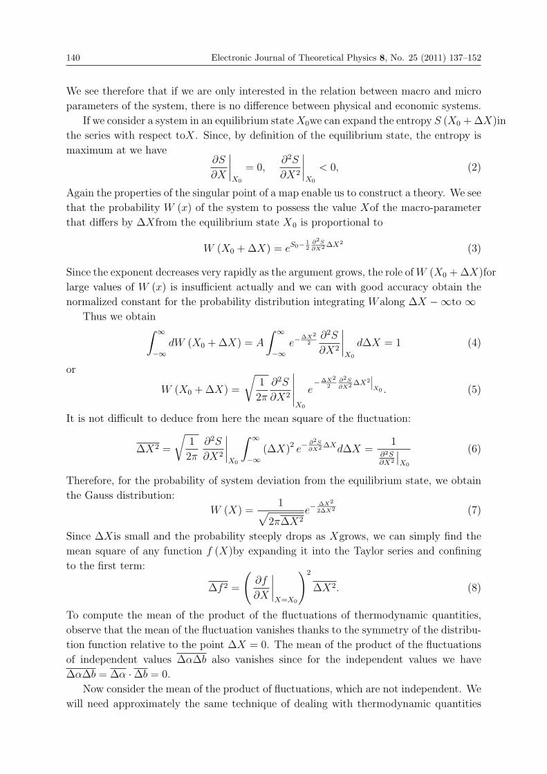
140 Electronic Journal of Theoretical Physics 8, No. 25 (2011) 137–152
We see therefore that if we are only interested in the relation between macro and micro
parameters of the system, there is no difference between physical and economic systems.
If we consider a system in an equilibrium stateX0we can expand the entropy S (X0 +ΔX)in
the series with respect toX. Since, by definition of the equilibrium state, the entropy is
maximum at we have∂S
∂X
∣∣∣∣X0
= 0,∂2S
∂X2
∣∣∣∣X0
< 0, (2)
Again the properties of the singular point of a map enable us to construct a theory. We see
that the probability W (x) of the system to possess the value Xof the macro-parameter
that differs by ΔXfrom the equilibrium state X0 is proportional to
W (X0 +ΔX) = eS0− 12
∂2S∂X2ΔX2
(3)
Since the exponent decreases very rapidly as the argument grows, the role ofW (X0 +ΔX)for
large values of W (x) is insufficient actually and we can with good accuracy obtain the
normalized constant for the probability distribution integrating Walong ΔX −∞to ∞Thus we obtain∫ ∞
−∞dW (X0 +ΔX) = A
∫ ∞
−∞e−
ΔX2
2∂2S
∂X2
∣∣∣∣X0
dΔX = 1 (4)
or
W (X0 +ΔX) =
√1
2π
∂2S
∂X2
∣∣∣∣∣X0
e−ΔX2
2∂2S∂X2ΔX2
∣∣∣X0 . (5)
It is not difficult to deduce from here the mean square of the fluctuation:
ΔX2 =
√1
2π
∂2S
∂X2
∣∣∣∣X0
∫ ∞
−∞(ΔX)2 e−
∂2S∂X2ΔXdΔX =
1∂2S∂X2
∣∣X0
(6)
Therefore, for the probability of system deviation from the equilibrium state, we obtain
the Gauss distribution:
W (X) =1√
2πΔX2e−
ΔX2
2ΔX2 (7)
Since ΔXis small and the probability steeply drops as Xgrows, we can simply find the
mean square of any function f (X)by expanding it into the Taylor series and confining
to the first term:
Δf 2 =
(∂f
∂X
∣∣∣∣X=X0
)2
ΔX2. (8)
To compute the mean of the product of the fluctuations of thermodynamic quantities,
observe that the mean of the fluctuation vanishes thanks to the symmetry of the distribu-
tion function relative to the point ΔX = 0. The mean of the product of the fluctuations
of independent values ΔαΔb also vanishes since for the independent values we have
ΔαΔb = Δα ·Δb = 0.
Now consider the mean of the product of fluctuations, which are not independent. We
will need approximately the same technique of dealing with thermodynamic quantities

Electronic Journal of Theoretical Physics 8, No. 25 (2011) 137–152 141
that we have already used to derive thermodynamic inequalities. If a fluctuation occurs
in a portion of the market, which is in equilibrium, this means that we can assume the
temperature of the universum and the price constants in the first approximation (for
a fluctuation). This in turn means that the deviations of the flow of money from the
equilibrium will be given by thermodynamic potential in accordance with arguments [8]
ΔΦ = ΔE − T0ΔS + P0ΔV (9)
where T0- is the equilibrium temperature and P0- is the equilibrium price.
Indeed, the entropy of the market is a function on the money flow. If we perform
a modification of this flow in a part of the system then the entropy of the system as a
whole will change:
ΔS =∂S
∂E· ΔE|P0T0
= T0ΔΦ. (10)
The changes of Φcan be found by expanding Einto the series with respect to δS and
δV .Observe here that the distribution function depends on the total change of the entropy
of the system under the fluctuation whereas δS and δV - are the changes of entropy and
the goods flow only for the separated part of the system.
In the same way as above we have
ΔΦ = ΔE − T0δS + P0δV
= 12
(∂2E∂S2 δS
2 + 2 ∂2E∂S∂V
δSδV + ∂2E∂V 2 δV
2)
= 12
(δSδ
(∂E∂V
∣∣S
))= 1
2(δSδT−δV δP )
(11)
Here we see the mathematical meaning of the variation of the thermodynamics potential
ΔΦ.It shows how much the money flow deviates from the tangent plane to the surface of
state E = E (V, T ).
Now we can express this change of ΔΦin varies coordinate system. Having selected
for example, the variables δV, δT we can express δS and δP in terms of δV, δT . After
implications we obtain
δPδV − δTδS = −CV
TδT 2 +
∂P
∂V
∣∣∣∣T
δV 2 (12)
The probability of fluctuation under the deviation of the systems from equilibrium is
accordingly proportional to the product of two factors depending on δV and δT
W (δT, δV ) ≈ e− 1
2T
(−CV
TδT 2+ ∂P
∂V |T δV 2)
(13)
i.e. δV δT = 0
It is not difficult to compute the mean quadratic values of the fluctuations by com-
paring W (δT, δV )with the Gauss distribution formula [9]
(δT )2 = T 2
CV,
(δT )2 = −T ∂V∂P
∣∣T
(14)

142 Electronic Journal of Theoretical Physics 8, No. 25 (2011) 137–152
This gives for the mean value of following value:
δPδT =
(∂P
∂V
∣∣∣∣T
δV − ∂P
∂T
∣∣∣∣V
δT
)δT =
∂P
∂V
∣∣∣∣T
δV 2 = −T (15)
This relation enables us to measure the temperature of the market by computing the
mean of the product of the fluctuation of the market by the fluctuation of the flow of
goods. Since the averaging over the ensemble can be replaced by averaging over time, we
obtain the following formula for the empirical computation of the market’s temperature:
T =1
2Tlim
∫ T
0
(V (t)− V
) (P (t)− P
)dt. (16)
Both the dependence of the price on time and the dependence of the flow of goods on
time are accessible, in principle, data, say, for the stock market. Therefore if we assume
that no external factors not determined by the structure of the market as such influence
the prices and the flows of goods then we have a means to measure thermodynamic
parameters of markets.
3. Fluctuation in Time
Here we consider the dependence of fluctuations on time in the system led out of the
equilibrium state. Observe here that we may only consider the not too large deviations
from equilibrium states but, on the other hand, not too small ones [10]
If the initial deviation of the equilibrium state is very tiny, the dynamics of the
fluctuations will not differ from the chaotic spontaneous fluctuations. If, on the other
hand, the initial deviation is very large, one has to take into account the non-linear effects
on the dependence on the speed of the deviation of the quantity under the study on the
value of the initial deviation.
Therefore we will confine ourselves to a linear case that is we will assume that in the
dependence of the speed with which the quantity returns to the equilibrium state on the
deviation we can ignore all the in the Taylor series expansion except the first one.
Speaking about practical applications of such an approach for prediction of behavior
of time series, say of the price on the share and stock markets this means that reasonable
predictions can be only made for short periods of time when the prices are still capable
to return to the equilibrium state but the time spans are still larger than the value of
dispersion.
In order to purely thermodynamic approach to work it is necessary that the “shadow of
future” does not affect too much the behavior of the market agents and the existence of a
certain symmetry between the sellers and the buyers. In other words, the thermodynamic
approach will hardly be effective for stock exchange, where the fulfillment of both of the
above requirements is hard to imagine but it can certainly be applicable for the commodity
markets.
In order to construct the theory of time fluctuations we have to introduce an important
value called autocorrelation function. It is defined as the average over the ensemble of

Electronic Journal of Theoretical Physics 8, No. 25 (2011) 137–152 143
the product of the values of the quantities studied separated by a fixed time interval
t0 and the time segments [tin , tik ](the subscripts n and k stand for the first letters of
Russian words “beginning” and “end” are the periods during which a prediction can be
significant. One can determine the value of dispersion of ΔX by means of the arguments
from the preceding section.
φ (t0) = 〈ΔX (t)ΔX (t+ t0)〉 . (17)
This quantity enables to determine the spectral density of the fluctuations, that is the
probability that the “frequency” of the fluctuation belongs to a certain interval. Here
speaking about “frequency” of fluctuations we use a metaphorical language because in
actual fact we have in mind the existence of processes with a certain characteristic relax-
ation time t0.
The frequency is inversely proportional to the relaxation time:
ω =1
t0(18)
In a more formal presentation, the arguments on a relation of the frequency of fluctuations
and the relaxation time are as follows. Consider the Fourier transform ofΔX (t):
ΔXω =1
2π
∞∫−∞
ΔX (t) eiωtdt. (19)
Then ΔX (t) can be considered as the inverse Fourier transform of ΔXω :
ΔX =
∞∫−∞
ΔXωe−iωtdω (20)
This expression for ΔX (t) can be substituted into the definition of the autocorrelation
function for ΔX (t):
φ (t0) =
⟨∫ ∞∫−∞
ΔXωΔXω′e−i(ω+ω′)te−iωt0dωdω′
⟩(21)
Now observe that, in accordance with the main principles of statistical thermodynamics,
the average over the ensemble can be replaced by averaging over time.
φ (t0) =
∫ ∞∫−∞
ΔXωΔXω′
⎛⎝ 1
T
T∫−T
e−i(ω+ω′)tdt
⎞⎠ e−iωt0dωdω′ (22)
In the limit as T → ∞the integral in parentheses become an expression for the delta
functionδ (ω+ω′). Therefore for the autocorrelation function φ (t0)we get the expression
φ (t0) =
∞∫−∞
ΔX2ωe−iωt0dω. (23)
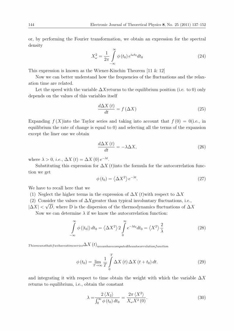
144 Electronic Journal of Theoretical Physics 8, No. 25 (2011) 137–152
or, by performing the Fourier transformation, we obtain an expression for the spectral
density
X2ω =
1
2π
∞∫−∞
φ (t0) eiωt0dt0 (24)
This expression is known as the Wiener-Kinchin Theorem [11 & 12]
Now we can better understand how the frequencies of the fluctuations and the relax-
ation time are related.
Let the speed with the variable ΔXreturns to the equilibrium position (i.e. to 0) only
depends on the values of this variables itself
dΔX (t)
dt= f (ΔX) (25)
Expanding f (X)into the Taylor series and taking into account that f (0) = 0(i.e., in
equilibrium the rate of change is equal to 0) and selecting all the terms of the expansion
except the liner one we obtain
dΔX (t)
dt= −λΔX, (26)
where λ > 0, i.e., ΔX (t) = ΔX (0) e−λt.Substituting this expression for ΔX (t)into the formula for the autocorrelation func-
tion we get
φ (t0) =⟨ΔX2
⟩e−λt. (27)
We have to recall here that we
(1) Neglect the higher terms in the expression of ΔX (t)with respect to ΔX
(2) Consider the values of ΔXgreater than typical involuntary fluctuations, i.e.,
|ΔX| <√D, where D is the dispersion of the thermodynamics fluctuations of ΔX
Now we can determine λ if we know the autocorrelation function:
∞∫−∞
φ (|t0|) dt0 =⟨ΔX2
⟩2
∞∫0
e−λt0dt0 =⟨X2
⟩ 2λ
(28)
ThismeansthatifwehaveatimeseriesΔX (t)wecanhavecomputedtheautocorrelationfunction
φ (t0) = limT→∞
1
T
T∫0
ΔX (t)ΔX (t+ t0) dt. (29)
and integrating it with respect to time obtain the weight with which the variable ΔX
returns to equilibrium, i.e., obtain the constant
λ =2 〈X2〉∫∞
0φ (t0) dt0
=2π 〈X2〉XωX2 (0)
. (30)

Electronic Journal of Theoretical Physics 8, No. 25 (2011) 137–152 145
where X2ω is the spectral density at zero frequency in accordance with the Wiener -
Kinchin theorem.
Observe that for the exponential autocorrelation function the spectral density is as
follows
X2ω =
λ
π (ω2 + λ2)
⟨X2
⟩. (31)
For frequencies smaller thanλ, the spectral density is approximately equal to 1πλ〈X2〉 ,
i.e., for the frequencies smaller than the inverse relaxation time of the system, we see that
the probabilities for ΔX to have such frequency component are approximately equal.
Observe that to apply the above theory of thermodynamic fluctuations to the study of
price relaxations on markets should be implemented with utmost caution for the reasons
that we consider in the next section.
4. The Collective Behavior at Market
Now we have to consider a very important question directly related with the study of
market fluctuations. How do fluctuations affect the perceptions of the market agents on
the future?
Generally speaking, the market agents have different information on the situation, it is
difficult to expect any coordinated behavior of the market agents anywhere, in particular,
in a neighborhood of the equilibrium. Indeed, the very lack of such a coordinated behavior
characterizes the “extended order” F. Hayek [13-15], wrote about. The one who discovers
new possibilities, new types of behavior gets an advantage and the multitude of such
possibilities is unlimited. Moreover it is unknown.
In the case when a certain stereotype of behavior starts to dominate one should not
expect the growth of “order”. Contrariwise, one should expect its destruction. This is
precisely what happens when a certain idea becomes common for a considerable majority
of market agents: for example to invest into a particular type of activity or company. In
this case, the shares quickly become overvalued and this sooner or later (usually relatively
soon) becomes clear thus influencing a new wave of spontaneously coordinated behavior,
this time to withdraw money from the corresponding activity.
Such situations lead not just to market fluctuations, but to considerable oscillations
and sometimes to a total transition of the market. Examples of this type are quite
numerous. It suffices to recall economic catastrophes in Mexico and South East Asia
during the 1990s.
A decisive role in such spontaneously coordinated behavior of the market agents is
played by the “shadow of future” that is, perceptions on a possible development of the
situation. The result turns out unexpected for the participants because their collective
behavior leads precisely to the very result that each of them tries to avoid.
A similar effect is well known in so-called non-cooperative games and is best studied
with an example of the game called “prisoner’s dilemma”. The innumerable literature
is devoted to this topic and here is not the place to discuss this problem, still observe

146 Electronic Journal of Theoretical Physics 8, No. 25 (2011) 137–152
that it is precisely in non-cooperative games (though in a somewhat different sense) the
radically important role of the “shadow of the future” in the molding of spontaneous
patterns of collective behavior have been singled out [16,17]
In this case the following problem becomes of interest: how are the small fluctuations
of the system related to patterns of spontaneous behavior that totally change the market
situation? In other words: what is the role of spontaneously formed collective behavior
in the problem of stability of market economy?
If small fluctuations of market parameters help to form spontaneous collective behav-
ior that destroys the market equilibrium then the market becomes evolutionary unstable
despite of the fact that in “neoclassical” sense such a market should possess equilibrium.
Lately similar questions are in the center of attention of researchers that try to leave
“neoclassical” orthodoxy and extend the frameworks of economic studies in particular
in connection with the study of the influence of technical innovations to economics [18].
Here we will confine ourselves to the simple model of “speculative behavior” which shows
under what conditions the market fluctuations can be considered as thermodynamic ones.
The study of the process of molding of the stock market price is of particular interest
both for creating forecasting models and from purely theoretical point of view since this
price is a good example illustrating how a directed activity of a multitude of people based
on individual forecasts and decision making leads to a formation of a certain collective
variable.
The problem of forecasting stock market prices requires a very detailed study of
the concrete situation and discovery of a number of factors not only of economic but
also of political character. An attempt of construction in mathematical model taking
into account all these factors is doomed to failure. Nevertheless observe that many of
external factors and also a number of economic factors (for example the level of actual
demand of an item of goods) may remain constant during a sufficiently long time though
the prices are subject to constant fluctuations. The reason for these fluctuations is a
speculative activity. Analysis of dependence of stock market prices on time shows us
that for sufficiently short lapses of time the nature of fluctuations often possesses certain
common peculiarities. This hints to study speculative oscillations provided the “long-
ranged” factors are constant. This makes it possible to model the modification of prices
making use of the difference in the “time scale” for price fluctuations caused by speculative
activities and oscillations resulting by “long-ranged” factors.
Let us abstract from the real conditions of stop market functioning making several
simplifications.
Define the “mean price” X (t)as the ratio of the mean amount of money P (t) spent
for the purchase of the goods per unit of time to the mean value of goods Q (t)sold at
the same time:
X (T ) =P (t)
Q (t)(32)
In the free market this ratio coincides with the marginal price that determines the market
equilibrium, where P (t) and Q (t)are slowly changing quantities whose value is deter-
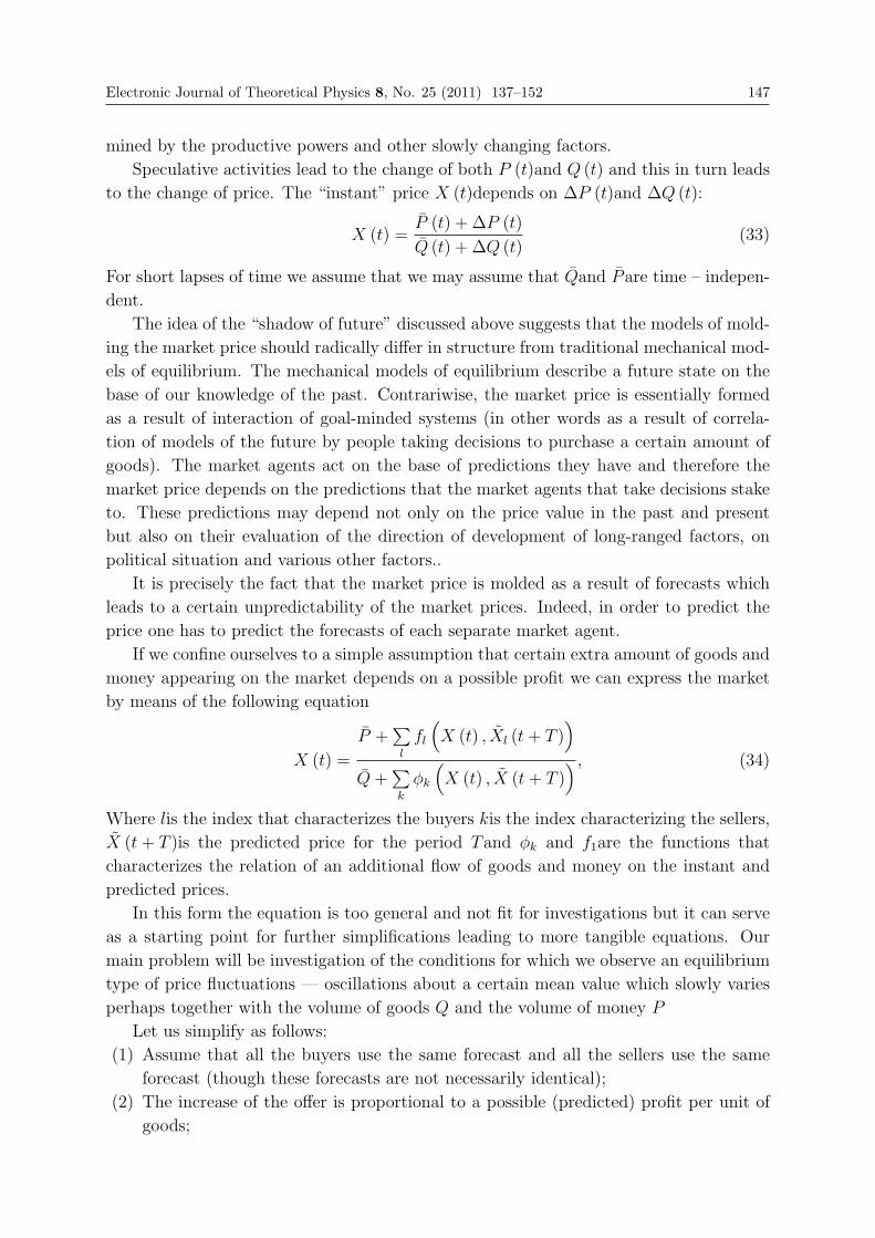
Electronic Journal of Theoretical Physics 8, No. 25 (2011) 137–152 147
mined by the productive powers and other slowly changing factors.
Speculative activities lead to the change of both P (t)and Q (t) and this in turn leads
to the change of price. The “instant” price X (t)depends on ΔP (t)and ΔQ (t):
X (t) =P (t) + ΔP (t)
Q (t) + ΔQ (t)(33)
For short lapses of time we assume that we may assume that Qand Pare time – indepen-
dent.
The idea of the “shadow of future” discussed above suggests that the models of mold-
ing the market price should radically differ in structure from traditional mechanical mod-
els of equilibrium. The mechanical models of equilibrium describe a future state on the
base of our knowledge of the past. Contrariwise, the market price is essentially formed
as a result of interaction of goal-minded systems (in other words as a result of correla-
tion of models of the future by people taking decisions to purchase a certain amount of
goods). The market agents act on the base of predictions they have and therefore the
market price depends on the predictions that the market agents that take decisions stake
to. These predictions may depend not only on the price value in the past and present
but also on their evaluation of the direction of development of long-ranged factors, on
political situation and various other factors..
It is precisely the fact that the market price is molded as a result of forecasts which
leads to a certain unpredictability of the market prices. Indeed, in order to predict the
price one has to predict the forecasts of each separate market agent.
If we confine ourselves to a simple assumption that certain extra amount of goods and
money appearing on the market depends on a possible profit we can express the market
by means of the following equation
X (t) =
P +∑l
fl
(X (t) , Xl (t+ T )
)Q+
∑k
φk
(X (t) , X (t+ T )
) , (34)
Where lis the index that characterizes the buyers kis the index characterizing the sellers,
X (t+ T )is the predicted price for the period Tand φk and f1are the functions that
characterizes the relation of an additional flow of goods and money on the instant and
predicted prices.
In this form the equation is too general and not fit for investigations but it can serve
as a starting point for further simplifications leading to more tangible equations. Our
main problem will be investigation of the conditions for which we observe an equilibrium
type of price fluctuations — oscillations about a certain mean value which slowly varies
perhaps together with the volume of goods Q and the volume of money P
Let us simplify as follows:
(1) Assume that all the buyers use the same forecast and all the sellers use the same
forecast (though these forecasts are not necessarily identical);
(2) The increase of the offer is proportional to a possible (predicted) profit per unit of
goods;

148 Electronic Journal of Theoretical Physics 8, No. 25 (2011) 137–152
(3) The increase of demand is also proportional to a possible profit.
Under these assumptions equation (34) takes the form
X (t) =P + α
(XP (t+ T )−X (t)
)Q+ β
(XQ (t+ θ)−X (t)
) , (35)
Where XP (t+ T )is the buyer’s prediction that use basis prediction time Tand XQ (t+ θ)is
the seller’s prediction that use the basis prediction timeθ
We should expect that Tand θmay be rather different, i.e., the market is, generally
speaking, asymmetric [19].
Let us simplify further. It is natural to assume that the prediction is determined by
the expansion of the price X (t) in the Taylor series with respect to time and terms higher
second order are neglected. It is difficult to conceive the influence of the derivatives of
the price greater than the second one on human perception: the eye usually catches the
first and second derivatives from the form of the curve. Thus the equation (35) takes the
form
X (t) =P + α
(TX + T 2
2X)
Q+ β(θX + θ2
2X) . (36)
We have the following alternatives:
(1) We may confine ourselves to the first derivatives thus obtaining the equation
X (t) =P + αTX
Q+ βθX; (37)
(1) We may study the more complicated equation (36)
Case (a) is rather simple. Resolving (37)
X =P − QX
BX − A, (38)
where B = βθ and A = αT .
Certainly one can integrated this equation but we will study it in a simply way. The
change of variables Z = BAXleads us to
FZ =Φ− Z
Z − 1, (39)
Where F = AQ, Φ = PB
QA.
If F > 0, that is A > 0 and Φ > 1, we have a stable equilibrium at the point
Z = Φ(X = P
Q
).
If F > 0and Φ < 1, then the equilibrium at Z = Φ(X = P
Q
)is unstable. Under a
small increase of the price it steeply up to the value corresponding to Z = 1(X = A
B
)and
under small diminishing falls to zero.

Electronic Journal of Theoretical Physics 8, No. 25 (2011) 137–152 149
The case Φ = 1is no equilibrium at all since Z = − 1F
(X = Q
B
).
For B < 0, the price continuously grows whereas B > 0it falls to zero.
In this situation every thing depends on the nature of the sellers’ forecast, i.e., do
they believe that the raising the price will stimulate the production or one should hide
the goals and wait till its price grows up.
Clearly, if the supplies are restricted or if there is a possibility to shrink the production,
the case B > 0is realized. In other words, in the case of a monopoly of the seller and
objective restrictions on supplies, the price grows unboundedly.
Apparently, this model adequately describes the phenomenon of sudden plummeting
of prices during social unrests and wars and also the inflation in the case of restricted
production.
Let us now consider another type of prognosis, which takes into account the second
derivative of price. Resolving equation (36) for the second derivative we get
X =P + αTX −X
(Q+ βθX
)β θ2
2X − αT 2
2
(40)
We may study this equation another by standard means, see, e.g., [9]. Introduce a new
variable X = Y and in the system of equation obtained eliminate time by dividing Xby
Y .
We get dYdX
=P+αTY−X(Q+βθY )
Y(β θ2
2X−αT2
2
) (40)
We can simplify this equation by setting
k1 = αT, k2 = αT 2
2, k3 = βθ, k4 = β
θ2
2. (41)
We getdY
dX=
P + QX
Y (k4X − k2)+
k1 − k3k4x− k2
(42)
Here we see that if k1 = k3then the system is equilibrium at the point Y = 0 that is
X = PQis the expected equilibrium point.
However, if k1 �= k3then X = PQis not an equilibrium point.
This is an astonishing result that shows that under asymmetric conditions taking into
account the second derivative we eliminate equilibrium. Asymmetric markets behave
totally unexpectedly.
Conclusion
From the above discussed the scope of the phenomenological analysis for Market Fluc-
tuations through Thermodynamics approach. Here we described how market parameters
vary with time by using of simplest example, and this extended to the market fluctuations
appears with the enforced changes of macro parameters of the market and land specu-
lations with non existence. And also we derived the equation for how market fluctuates
150 Electronic Journal of Theoretical Physics 8, No. 25 (2011) 137–152
with respect to time in an equilibrium state. Finally we analyzed the how the fluctuations
affects the perceptions of the market agents on the future.
From the above discussion our considerations resulted in rather unexpected corol-
laries: The “shadow of future” for the linear forecast restricts the domain of a stable
equilibrium but even for the asymmetric forecasts of sellers and buyers it does not totally
eliminate the equilibrium. Adding the second derivative into the forecast (which amounts,
actually, to professionalization of the forecast) completely eliminates equilibrium for the
asymmetric markets. In other words, the market becomes globally unstable. This de-
duction is extremely important for our further analysis. It means that there appears a
possibility to manipulate the market using restricted resources
References
[1] G. Guillaume, E. Guillaume, Sur le fundaments de l’economique rationelle, Gautier-Villars, Paris, 1932.
[2] P. Samuelson, Collected Economics Papers, Vol. 5, MIT Pr., Cambridge, 1986.
[3] P. Mirowski, Machine Dreams, Cambridge, Cambridge, 2002.
[4] E. Smith, D.K. Foley, Is utility theory so different from thermodynamics? SFIpreprint, 2002.
[5] D. Ruelle, Statistical Mechanics, Thermodynamic Formalism, Addison-Wesley,Reading, Mass., 1978.
[6] P. Cvitanovic, G.H. Gunaratne, I. Procaccia, Phys. Rev. A38 (1988) 1503.
[7] J.L. McCauley, Classical Mechanics: flows, transformations, integrability and chaos,Cambridge, Cambridge, 1997.
[8] Landau L. D., Lifshitz E. M. Course of theoretical physics. Vol. 5: Statistical physics.Translated from the Russian by J.B. Sykes and M. J. Kearsley. Second revised andenlarged edition Pergamon Press, Oxford-Edinburgh-New York, 1968, xii+484 pp.
[9] Tricomi F. G., Differential equations. Translated by Elizabeth A. McHarg HafnerPublishing Co., New York 1961 x+273 pp.
[10] Mills T. C., The Econometric Modeling of Financial Time Series. Cambridge Univ.Press, Cambridge, 1993.
[11] Wiener, N., The Fourier integral and certain of its applications. Reprint of the 1933edition. With a foreword by Jean-Pierre Kahane. Cambridge Mathematical Library.Cambridge University Press, Cambridge, 1988. xviii+201 pp.
[12] Wiener, N., Nonlinear problems in random theory. Technology Press ResearchMonographs The Technology Press of The Massachusetts Institute of Technologyand John Wiley & Sons, Inc., New York; Chapman & Hall, Ltd., London 1958.ix+131 pp.
[13] Hayek F. A. The Road to Serfdom. Chicago Univ. Press, Chicago, 1977
[14] Hayek F. A. New Studies in Philosophy, Politics, Economics and the History ofIdeas,Chicago Univ. Press, Chicago, 1978
[15] Hayek F. A. The Fatal Conceit. In: Collected Works of F.A. Hayek. University ofChicago Press, Chicago, 1988

Electronic Journal of Theoretical Physics 8, No. 25 (2011) 137–152 151
[16] Axelrod R. The Evolution of Cooperation. New York, Basic, 1984
[17] Sergeev V., The Wild East (Crime and lawlessness in post-Soviet Russia), M. E.Sharp Armonk, NY, 1998
[18] Arthur W.B. Self-reinforcing mechanisms in Economics. In: P. W. Anderson, K. J.Arrow, D. Pines (eds.) The Economy as an Evolving Complex System. Proceedingsof the Workshop on the Evolutionary Paths of the Global Economy Held in Santa Fe,New Mexico, September, 1987. Addison-Wesley, Redwood City, CA, 1988, 9 – 31.
[19] Akerloff G.A. The Market for Lemons: Qualitative Uncertainty and the MarketMechanism. Quaterly J. Econom., 1970, 84, 488–500.

EJTP 8, No. 25 (2011) 153–168 Electronic Journal of Theoretical Physics
Magnetized Bianchi Type V I0 Bulk ViscousBarotropic Massive String Universe with Decaying
Vacuum Energy Density Λ
Anirudh Pradhan∗1 and Suman Lata 2
1,2Department of Mathematics, Hindu Post-graduate College, Zamania-232 331,Ghazipur, India
2Department of Mathematics, G. G. I. C., Ghazipur-233 001, India
Received 6 July 2010, Accepted 10 February 2011, Published 25 May 2011
Abstract: Bianchi type V I0 bulk viscous massive string cosmological models using the
technique given by Letelier (1983) with magnetic field are investigated. To get the deterministic
models, we assume that the expansion (θ) in the model is proportional to the shear (σ) and also
the fluid obeys the barotropic equation of state. The viscosity coefficient of bulk viscous fluid
is assumed to be a power function of mass density. The value of the vacuum energy density Λ
is observed to be small and positive at late time which is supported from recent supernovae Ia
observations. The behaviour of the models from physical and geometrical aspects in presence
and absence of magnetic field is also discussed.c© Electronic Journal of Theoretical Physics. All rights reserved.
Keywords: Massive String; Bianchi type V I0 Universe, Variable Λ; Bulk viscosity
PACS (2010): 11.10.-z; 98.80.Cq; 04.20.-q; 98.80.-k
1. Introduction
The problem of the cosmological constant is one of the most salient and unsettled prob-
lems in cosmology. The smallness of the effective cosmological constant recently observed
(Λ0 ≤ 10−56cm−2) constitutes the most difficult problems involving cosmology and ele-
mentary particle physics theory. To explain the striking cancellation between the “bare”
cosmological constant and the ordinary vacuum energy contributions of the quantum
fields, many mechanisms have been proposed during last few years [1]. The “cosmologi-
cal constant problem” can be expressed as the discrepancy between the negligible value
of Λ has for the present universe (as can be seen by the successes of Newton’s theory
∗ E-mail: [email protected], [email protected]

154 Electronic Journal of Theoretical Physics 8, No. 25 (2011) 153–168
of gravitation [2]) and the values 1050 larger expected by the Glashow-Salam-Weinberg
model [3] or by grand unified theory (GUT) where it should be 10107 larger [4]. The
cosmological term Λ is then small at the present epoch. The problem in this approach
is to determine the right dependence of Λ upon S or t. Recent observations of Type
Ia supernovae (Perlmutter et al. [5], Riess et al. [6]) and measurements of the cosmic
microwave background [7] suggest that the universe is an accelerating expansion phase [8].
Several ansatz have been proposed in which the Λ term decays with time (see Refs.
Gasperini [9], Berman [10-12], Berman et al. [13-15], Freese et al. [16], Ozer and Taha
[17], Ratra and Peebles [18], Chen and Hu [19], Abdussattar and Vishwakarma [20], Gariel
and Le Denmat [21], Pradhan et al. [22]). Of the special interest is the ansatz Λ ∝ S−2
(where S is the scale factor of the Robertson-Walker metric) by Chen and Wu [19], which
has been considered/modified by several authors ( Abdel-Rahaman [23], Carvalho et al.
[24], Silveira and Waga [25], Vishwakarma [26]).
One of the outstanding problems in cosmology today is developing a more precise
understanding of structure formation in the universe, that is, the origin of galaxies and
other large-scale structures. Existing theories for the structure formation of the Universe
fall into two categories, based either upon the amplification of quantum fluctuations in
a scalar field during inflation, or upon symmetry breaking phase transition in the early
Universe which leads to the formation of topological defects such as domain walls, cosmic
strings, monopoles, textures and other ’hybrid’ creatures. Cosmic strings play an impor-
tant role in the study of the early universe. These arise during the phase transition after
the big bang explosion as the temperature goes down below some critical temperature
as predicted by grand unified theories (see Refs. Zel’dovich et al. [27], Kibble [28, 29],
Everett [30], Vilenkin [31]). It is believed that cosmic strings give rise to density pertur-
bations which lead to formation of galaxies (Zel’dovich [32]). These cosmic strings have
stress energy and couple to the gravitational field. Therefore, it is interesting to study
the gravitational effect which arises from strings. The general treatment of strings was
initiated by Letelier [33, 34] and Stachel [35].
The occurrence of magnetic fields on galactic scale is well-established fact today, and
their importance for a variety of astrophysical phenomena is generally acknowledged.
Several authors (Zeldovich [36], Harrison [37], Misner, Thorne and Wheeler [38], Asseo
and Sol [39], Pudritz and Silk [40], Kim, Tribble, and Kronberg [41], Perley, and Taylor
[42], Kronberg, Perry, and Zukowski [43], Wolfe, Lanzetta and Oren [44], Kulsrud, Cen,
Ostriker and Ryu [45] and Barrow [46]) have pointed out the importance of magnetic
field in different context. As a natural consequences, we should include magnetic fields in
the energy-momentum tensor of the early universe. The string cosmological models with
a magnetic field are also discussed by Benerjee et al. [47], Chakraborty [48], Tikekar and
Patel ([49], Patel and Maharaj [51] Singh and Singh [52].

Electronic Journal of Theoretical Physics 8, No. 25 (2011) 153–168 155
Recently, Bali et al. [53-57], Pradhan et al. [58-60], Yadav et al. [61] and Pradhan [62]
have investigated Bianchi type I, II, III, V, IX and cylindrically symmetric magnetized
string cosmological models in presence and absence of magnetic field. Pradhan and
Bali [50] have investigated some solutions for Bianchi type V I0 cosmology in presence
and absence of magnetic field. In this paper we have derived some Bianchi type V I0string cosmological models for bulk viscous fluid distribution in presence and absence of
magnetic field and discussed the variation of Λ with time. This paper is organized as
follows: The metric and field equations are presented in Section 2. In Section 3, we deal
with the solution of the field equations in presence of magnetic field. In Section 4, we
have described the solution of the field equations in presence of bulk viscous fluid and
some geometric and physical behaviour of the model. Section 5 includes the solution in
absence of magnetic field. In Section 6, we hav discussed the bulk viscous solution of the
field equations in absence of magnetic field. In the last Section 7, concluding remarks are
given.
2. The Metric and Field Equations
We consider the Bianchi Type V I0 metric in the form
ds2 = −dt2 + A2(t)dx2 +B2(t)e2xdy2 + C2(t)e−2xdz2. (1)
The energy-momentum tensor for a cloud of strings in presence of magnetic field is taken
into the form
Tik = (ρ+ p)vivk + pgik − λxixk + [glmFilFkm −1
4gikFlmF
lm], (2)
where vi and xi satisfy conditions
vivi = −xixi = −1, vixi = 0. (3)
In equations (2), p is isotropic pressure, ρ is rest energy density for a cloud strings, λ is
the string tension density, Fij is the electromagnetic field tensor, xi is a unit space-like
vector representing the direction of string, and vi is the four velocity vector satisfying the
relation
gijvivj = −1. (4)
Here, the co-moving coordinates are taken to be v1 = 0 = v2 = v3 and v4 = 1 and
xi = ( 1A, 0, 0, 0). The Maxwell’s equations
Fij;k + Fjk;i + Fki;j = 0, (5)
F ik;k = 0, (6)
are satisfied by
F23 = K(say) = constant, (7)

156 Electronic Journal of Theoretical Physics 8, No. 25 (2011) 153–168
where a semicolon (;) stands for covariant differentiation.
The Einstein’s field equations (with 8πGc4
= 1)
Rji −
1
2Rgji = −T j
i − Λgji , (8)
for the line-element(1) lead to the following system of equations:
B44
B+C44
C+B4C4
BC+
1
A2= −
[p− λ− K2
2B2C2
]− Λ, (9)
A44
A+C44
C+A4C4
AC− 1
A2= −
[p+
K2
2B2C2
]− Λ, (10)
A44
A+B44
B+A4B4
AB− 1
A2= −
[p+
K2
2B2C2
]− Λ, (11)
A4B4
AB+B4C4
BC+C4A4
CA− 1
A2=
[ρ+
K2
2B2C2
]− Λ, (12)
1
A
[C4
C− B4
B
]= 0, (13)
where the sub indice 4 in A, B, C denotes ordinary differentiation with respect to t. The
velocity field vi is irrotational. The scalar expansion θ and components of shear σij are
given by
θ =A4
A+B4
B+C4
C, (14)
σ11 =A2
3
[2A4
A− B4
B− C4
C
], (15)
σ22 =B2
3
[2B4
B− A4
A− C4
C
], (16)
σ33 =C2
3
[2C4
C− A4
A− B4
B
], (17)
σ44 = 0. (18)
Therefore
σ2 =1
2
[(σ1
1)2 + (σ2
2)2 + (σ3
3)2 + (σ4
4)2
],
which leads to
σ2 =1
3
[A2
4
A2+B2
4
B2+C2
4
C2− A4B4
AB− B4C4
BC− C4A4
CA
].
Above relation after using (13) reduces to
σ =1√3
(A4
A− B4
B
). (19)

Electronic Journal of Theoretical Physics 8, No. 25 (2011) 153–168 157
3. Solutions of the Field Equations
We have revisted the solutions obtained by Pradhan and Bali [50]. The field equations
(9)-(13) are a system of five equations with seven unknown parameters A, B, C, ρ, p, λ
and Λ. We need two additional conditions to obtain explicit solutions of the system.
Equation (13) leads to
C = mB, (20)
where m is an integrating constant.
We first assume that the expansion (θ) in the model is proportional to shear (σ). The
motive behind assuming this condition is explained with reference to Thorne [63], the ob-
servations of the velocity-red-shift relation for extragalactic sources suggest that Hubble
expansion of the universe is isotropic today within ≈ 30 per cent [64, 65]. To put more
precisely, red-shift studies place the limit
σ
H≤ 0.3
on the ratio of shear, σ, to Hubble constant, H, in the neighbourhood of our Galaxy today.
Collins et al. [66] have pointed out that for spatially homogeneous metric, the normal
congruence to the homogeneous expansion satisfies that the condition σθis constant. This
condition and Eq. (20) lead to
1√3
(A4
A− B4
B
)= l
(A4
A+2B4
B
)(21)
which yields toA4
A= n
B4
B, (22)
where n = (2l√3+1)
(1−l√3)and l are constants. Eq. (22), after integration, reduces to
A = βBn, (23)
where β is a constant of integration. Eqs. (10) and (12) lead to
p = − K2
2B2C2−
(A44
A+C44
C+A4C4
AC− 1
A2
)− Λ, (24)
and
ρ =A4B4
AB+B4C4
BC+C4A4
CA− 1
A2− K2
2B2C2+ Λ, (25)
respectively. Now let us consider that the fluid obeys the barotropic equation of state
p = γρ, (26)
where γ(γ ≤ 0 ≤ 1) is a constant. Eqs. (24) to (26) lead to
A44
A+C44
C+ (1 + γ)
A4C4
AC+ γ
(A4B4
AB+B4C4
BC
)− (1 + γ)
1
A2+

158 Electronic Journal of Theoretical Physics 8, No. 25 (2011) 153–168
(1− γ)K2
2B2C2+ (1 + γ)Λ = 0. (27)
Eq. (27) with the help of (20) and (23) reduces to
2B44 +2(n2 + 2γn+ γ)
(n+ 1)
B24
B2=2(1 + γ)
β2B2n−1 +(1− γ)K2
m2B3+ 2l0B, (28)
where l0 = (1 + γ)Λ.
Let us consider B4 = f(B) and f ′ = dfdB. Hence Eq. (28) takes the form
d
df(f 2) +
2α
Bf 2 =
2(1 + γ)
β2B2n−1 +(1− γ)K2
m2B3+ 2l0B, (29)
where α = (n2+2nγ+γ)(n+1)
. Eq. (29) after integrating reduces to
f 2 =2(1 + γ)B−2n+2
β2(2α− 2n+ 2)+
(1− γ)K2
2m2(α− 1)+
l0B2
(α + 1)+MB−2α, γ �= 1, (30)
where M is an integrating constant. To get deterministic solution in terms of cosmic
string t, we suppose M = 0 without any loss of generality. In this case Eq. (30) takes
the form
f 2 = aB−2(n−1) + bB−2 + kB2, (31)
where
a =2(1 + γ)
β2(2α− 2n+ 2), b =
(1− γ)K2
2m2(α− 1), k =
(1 + γ)Λ
(α + 1).
Therefore, we havedB√
aB−2(n−1) + bB−2 + kB2= dt. (32)
To get deterministic solution, we assume n = 2. In this case integrating Eq. (32), we
obtain
B2 =√(a+ b)
sinh (2√kt)√
k. (33)
Hence, we have
C2 = m2√(a+ b)
sinh (2√kt)√
k, (34)
A2 = β2(a+ b)sinh2 (2
√kt)
k, (35)
where k > 0 without any loss of generality.
Therefore, the metric (1), in presence of magnetic field, reduces to the form
ds2 = −dt2 + β2(a+ b)sinh2 (2
√kt)
kdx2+

Electronic Journal of Theoretical Physics 8, No. 25 (2011) 153–168 159
√(a+ b)
sinh (2√kt)√
ke2x dy2 +m2
√(a+ b)
sinh (2√kt)√
ke−2x dz2. (36)
The expressions for the pressure (p), energy density (ρ), the string tension density
(λ), the particle density (ρp) for the model (36) are given by
p =
[k
β2(a+ b)− K2k
2m2(a+ b)
]coth2 (2
√kt)+
[K2
2m2(a+ b)− 1
β2(a+ b)− 8
]k − Λ, (37)
ρ =
[5k − k
(a+ b)
(K2
2m2+
1
β2
)]coth2 (2
√kt)+
k
(a+ b)
(K2
2m2+
1
β2
)+ Λ, (38)
where p = γρ is satisfied by (27).
λ =
[2k
β2(a+ b)− K2k
m2(a+ b)− k
]coth2 (2
√kt)+
{K2k
m2(a+ b)− 2k
β2(a+ b)− 4k
}, (39)
ρp = ρ− λ =
[K2k
2m2(a+ b)− 3k
β2(a+ b)+ k
]coth2 (2
√kt)
+9k +
{3k
β2(a+ b)− K2
2m2(a+ b)
}, (40)
4. Solutions for Bulk Viscous Fluid
Astronomical observations of large-scale distribution of galaxies of our universe show
that the distribution of matter can be satisfactorily described by a perfect fluid. But
large entropy per baryon and the remarkable degree of isotropy of the cosmic microwave
background radiation, suggest that we should analyze dissipative effects in cosmology.
Further, there are several processes which are expected to give rise to viscous effect.
These are the decoupling of neutrinos during the radiation era and the recombination era
[67], decay of massive super string modes into massless modes [68], gravitational string
production [69, 70] and particle creation effect in grand unification era [71]. It is known
that the introduction of bulk viscosity can avoid the big bang singularity. Thus, we
should consider the presence of a material distribution other than a perfect fluid to have
realistic cosmological models (see Grøn [72] for a review on cosmological models with

160 Electronic Journal of Theoretical Physics 8, No. 25 (2011) 153–168
bulk viscosity). A uniform cosmological model filled with fluid which possesses pressure
and second (bulk) viscosity was developed by Murphy [73]. The solutions that he found
exhibit an interesting feature that the big bang type singularity appears in the infinite
past.
In presence of bulk viscous fluid distribution, we replace isotropic pressure p by effective
pressure p in Eq. (37) where
p = p− ξvi;i, (41)
where ξ is the coefficient of bulk viscosity.
The scalar of expansion (θ) for the model (36) is given by
θ = 4√k coth (2
√kt), (42)
The expression for effective pressure p for the model Eq. (36) is given by
p = (p− ξvi;i) =
[k
β2(a+ b)− K2k
2m2(a+ b)
]coth2 (2
√kt)
+
[K2
2m2(a+ b)− 1
β2(a+ b)− 8
]k − Λ, (43)
Thus, for given ξ(t) we can solve for the cosmological parameters. In most of the inves-
tigation involving bulk viscosity is assumed to be a simple power function of the energy
density (Pavon [74], Maartens [75], Zimdahl [76], Santos [77])
ξ(t) = ξ0ρn, (44)
where ξ0 and n are constants. For small density, n may even be equal to unity as used
in Murphy’s work [52] for simplicity. If n = 1, Eq. (43) may correspond to a radiative
fluid (Weinberg [2]). Near the big bang, 0 ≤ n ≤ 12is a more appropriate assumption
(Belinskii and Khalatnikov [78]) to obtain realistic models.
For simplicity sake and for realistic models of physical importance, we consider the
following two cases (n = 0, 1):
4.1 Model I: When n = 0
When n = 0, Eq. (44) reduces to ξ = ξ0 = constant. With the use of Eqs. (37), (26) and
(42), Eq. (43) reduces to
(1 + γ)ρ = 4ξ0√k coth (2
√kt) + (5k − k1 + k2) coth
2 (2√kt) + (k1 − k2), (45)
where
k1 =k
(a+ b)
(K2
2m2+
1
β2
),
Electronic Journal of Theoretical Physics 8, No. 25 (2011) 153–168 161
and
k2 =k
(a+ b)
(1
β2− K2
2m2
).
Eliminating ρ(t) between Eqs. (38) and (45), we obtain
(1 + γ)Λ = 4ξ0√k coth (2
√kt) + [k2 − (5k − k1)γ] coth
2 (2√kt)− (k1γ + k2). (46)
4.2 Model II: When n = 1
When n = 1, Eq. (44) reduces to ξ = ξ0ρ. With the use of Eqs. (37), (26) and (42), Eq.
(43) reduces to
ρ =(5k − k1 + k2) coth (2
√kt) + (k1 − k2)
[1 + γ − 4ξ0√k coth (2
√kt)]
. (47)
Eliminating ρ(t) between Eqs. (38) and (47), we obtain
Λ =(5k − k1 + k2) coth (2
√kt) + (k1 − k2)
[1 + γ − 4ξ0√k coth (2
√kt)]
− (5k − k1) coth (2√kt)− k1. (48)
From Eqs. (45) and (47), by choosing the appropriate values of constant quantities, we
observe that ρ(t) in both models are a decreasing function of time and ρ > 0 for all times.
From Eqs. (46) and (48), we see that the cosmological terms Λ in both models are a
decreasing function of time and they approach a small positive value at late time. Thus,
our models are consistent with the results of recent observations (Perlmutter et al. [5],
Riess et al. [6]).
The effect of bulk viscosity is to produce a change in perfect fluid and therefore ex-
hibits essential influence on the character of the solution. A comparative inspection of
ρ show apparent evolution of time due to perfect fluid and bulk viscous fluid. It is ap-
parent that the vacuum energy density (ρ) decays much fast in later case. Also shows
effect of uniform viscosity model and linear viscosity model. Even in these case decay of
vacuum energy density is much faster than uniform. So the coupling parameter ξ0 would
be related with physical structure of the matter and provides mechanism to incorporate
relevant property. In order to say more specific, detailed study would be needed which
would be reported in future. Similar behaviour is observed for the cosmological constant
Λ. We also observe here that Murphy’s [73] conclusion about the absence of a big bang
type singularity in the infinite past in models with bulk viscous fluid in general, is not
true. The results obtained by Myung and Cho [68] also show that, it is not generally
valid since for some cases big bang singularity occurs in finite past.
The shear tensor (σ) and the proper volume (V 3) for the model (36) are given by
σ =
√k
3coth (2
√kt), (49)

162 Electronic Journal of Theoretical Physics 8, No. 25 (2011) 153–168
V 3 =βm(a+ b)
ksinh2 (2
√kt). (50)
From Eqs. (42) and (49), we obtain
σ
θ= constant. (51)
The deceleration parameter is given by
q = − R/R
R2/R2= −
[8k3− 8k
9coth2 (2
√kt)
16k9coth2 (2
√kt)
]. (52)
From (52), we observe that
q < 0 if coth2 (2√kt) < 3
and
q > 0 if coth2 (2√kt) > 3.
From (38), ρ ≥ 0 implies that
coth2 (2√kt) ≤
[ k(a+b)
(K2
2m2 +1β2
)+ Λ
k(a+b)
(K2
2m2 +1β2
)− 5k
]. (53)
Also from (40), ρp ≥ 0 implies that
coth2 (2√kt) ≤
[ 3kβ2(a+b)
− K2
2m2(a+b)+ 9k
3kβ2(a+b)
− K2k2m2(a+b)
− k
]. (54)
Thus the energy conditions ρ ≥ 0, ρp ≥ 0 are satisfied under conditions given by (53)
and (54).
The model (36) starts with a big bang at t = 0. The expansion in the model decreases
as time increases. The proper volume of the model increases as time increases. Sinceσθ= constant, hence the model does not approach isotropy. Since ρ, λ, θ, σ tend to
infinity and V 3 → 0 at initial epoch t = 0, therefore, the model (36) for massive string
in presence of magnetic field has Line-singularity (Banerjee et al. [47]). For the condi-
tion coth2 (2√kt) < 3, the solution gives accelerating model of the universe. It can be
easily seen that when coth2 (2√kt) > 3, our solution represents decelerating model of the
universe.
5. Solutions in Absence of Magnetic Field
In absence of magnetic field, i.e. when b→ 0 i.e. K → 0, we obtain
B2 = 2√2sinh (2
√kt)
2√k
,

Electronic Journal of Theoretical Physics 8, No. 25 (2011) 153–168 163
C2 = 2m2√asinh (2
√kt)
2√k
,
A2 = 4aβ2 sinh2 (2√kt)
4k. (55)
Hence, in this case, the geometry of the universe (36) reduces to
ds2 = −dt2 + 4β2asinh2 (2
√kt)
4kdx2+
2√2sinh (2
√kt)
2√k
e2x dy2 + 2m2√asinh (2
√kt)
2√k
e−2x dz2. (56)
The pressure (p), energy density (ρ), the string tension density (λ), the particle density
(ρp), the scalar of expansion (θ) for the model (56) are given by
p =k
aβ2coth2 (2
√kt)−
(1
aβ2+ 8
)k − Λ, (57)
ρ =
(5k − k
aβ2
)coth2 (2
√kt) +
k
aβ2+ Λ, (58)
λ =
[2k
aβ2− k
]coth2 (2
√kt)−
{2k
aβ2+ 4k
}, (59)
ρp = ρ− λ =
[k − 3k
aβ2
]coth2 (2
√kt) + 9k +
3k
β2a, (60)
θ = 4√k coth (2
√kt), (61)
6. Solutions for Bulk Viscous Fluid
The expression for effective pressure p for the model Eq. (56) is given by
p = (p− ξvi;i) =k
aβ2coth2 (2
√kt)−
(1
aβ2+ 8
)k − Λ (62)
Thus, for given ξ(t) we can solve for the cosmological parameters. For simplicity sake and
for realistic models of physical importance, we consider the following two cases (n = 0, 1):
6.1 Model I: When n = 0
When n = 0, Eq. (44) reduces to ξ = ξ0 = constant. With the use of Eqs. (57), (26) and
(61), Eq. (62) reduces to
(1 + γ)ρ = 4ξ0√k coth (2
√kt) + 5k coth2 (2
√kt)− 8k (63)
Eliminating ρ(t) between Eqs. (58) and (63), we obtain
(1 + γ)Λ = 4ξ0√k coth (2
√kt)− [5γ +
(1 + γ)
aβ2]k coth2 (2
√kt)− (1 + γ)k
aβ2(64)
164 Electronic Journal of Theoretical Physics 8, No. 25 (2011) 153–168
6.2 Model II: When n = 1
When n = 1, Eq. (44) reduces to ξ = ξ0ρ. With the use of Eqs. (57), (26) and (61), Eq.
(62) reduces to
ρ =5k coth (2
√kt) + 8k
[1 + γ + 4ξ0√k coth (2
√kt)]
. (65)
Eliminating ρ(t) between Eqs. (58) and (65), we obtain
Λ =5k coth (2
√kt) + 8k
[1 + γ + 4ξ0√k coth (2
√kt)]
− [5− 1
aβ2]k coth (2
√kt)− k
aβ2. (66)
From Eqs. (63) and (65), by choosing the proper values of constant quantities, we observe
that ρ(t) in both models are a decreasing function of time and ρ > 0 for all times. From
Eqs. (64) and (66), we see that the cosmological terms Λ in both models are a decreasing
function of time and they approach a small positive value at late time. Thus, our models
are consistent with the results of recent observations (Perlmutter et al. [5], Riess et al.
[6]).
The shear tensor (σ) and the proper volume (V 3) for the model (49) are given by
σ =
√k
3coth (2
√kt), (67)
V 3 =βma
ksinh2 (2
√kt). (68)
From Eqs. (61) and (67), we obtain
σ
θ= constant. (69)
From (58), ρ ≥ 0 implies that
coth2 (2√kt) ≤
[ kaβ2 + Λk
aβ2 − 5k
]. (70)
Also from (60), ρp ≥ 0 implies that
coth2 (2√kt) ≤
[ 3kaβ2 + ak3kaβ2 − k
]. (71)
Thus the energy conditions ρ ≥ 0, ρp ≥ 0 are satisfied under conditions given by (70)
and (71).
The model (56) starts with a big bang at t = 0 and the expansion in the model
decreases as time increases. The spatial volume of the model increases as time increases.
Since σθ= constant, hence the anisotropy is maintained throughout. Since ρ, λ, θ, σ tend
to infinity and V 3 → 0 at initial epoch t = 0, therefore, the model (56) for massive string
in absence of magnetic field has Line-singularity [47].

Electronic Journal of Theoretical Physics 8, No. 25 (2011) 153–168 165
Concluding Remarks
Some Bianchi type V I0 massive string cosmological models with a bulk viscous fluid as
the source of matter are obtained in presence and absence of magnetic field. Generally,
the models are expanding, shearing and non-rotating. In presence of bulk viscous fluid
it represents an accelerating universe during the span of time mentioned below equation
(52) as decelerating factor q < 0 and it represents decelerating universe as q > 0. All
the two massive string cosmological models obtained in the present study have Line-
singularity (Banerjee et al. [47]) at the initial epoch t = 0. The variation of cosmological
term in presence and absence of magnetic field is consistent with recent observations. To
solve the age parameter and density parameter, one requires the cosmological constant
to be positive or equivalently the deceleration parameter to be negative. The nature of
the cosmological constant Λ and the energy density ρ have been examined.
We have also observed that the magnetic field gives positive contribution to expansion
and shear which die out for large value of t at a slower rate than the corresponding quan-
tities in the absence of magnetic field. In our derived models, in presence and absence
of magnetic field, by proper choice of the constant quantities the cosmological term Λ
are found to be a decreasing function of time and their values approach a small positive
value at late time which is supported by recent results from the observations of Type
Ia supernova explosion (SN Ia). Naturally a cosmological model is required to explain
acceleration in the present universe. Thus, our theoretical models are consistent with the
results of recent observations.
The effect of bulk viscosity is to produce a change in perfect fluid and therefore exhibits
essential influence on the character of the solution. The effect is clearly visible on the p
effective (see details in previous sections). We have observed regular well behaviour of
energy density, cosmological term (Λ) and the expansion of the universe with parameter
t in both presence and absence of magnetic field. Our solutions generalize the solutions
recently obtained by Pradhan and Bali [50].
Acknowledgement
One of the authors (A. Pradhan) thanks the Institute of Mathematical Science (IMSc.),
Chennai, India for providing facility and hospitality under associateship scheme where
part of this work was carried out.
References
[1] S. Weinberg, Rev. Mod. Phys. 61, 1 (1989).
[2] S. Weinberg, Gravitation and Cosmology, Wiley, New York, 1972.
[3] E. S. Abers and B. W. Lee, Phys. Rep. 9, 1 (1973).

166 Electronic Journal of Theoretical Physics 8, No. 25 (2011) 153–168
[4] P. Langacker, Phys. Rep. 72, 185 (1981).
[5] S. Perlmutter et al., Astrophys. J. 483, 565 (1997) (astro-ph/9608192).S. Perlmutter et al., Nature 391, 51 (1998) (astro-ph/9712212);S. Perlmutter et al., Astrophys. J. 517, 5 (1999)(astro-ph/9812133).
[6] A. G. Riess et al., Astron. J. 116 (1998) 1009 (astro-ph/9805201).A. G. Riess: PASP, 114 1284 (2000).
[7] P. De Bernardis et al., Ap. J. 564, 559 (2002).
[8] S. M. Caroll, astro-ph/0310342 (2003).
[9] M. Gasperini, Phys. Lett. B 194, 347 (1987).M. Gasperini, Class. Quant. Grav. 5, 521 (1988).
[10] M. S. Berman, Int. J. Theor. Phys. 29, 567 (1990).
[11] M. S. Berman, Int. J. Theor. Phys. 29, 1419 (1990).
[12] M. S. Berman, Phys. Rev. D 43, 75 (1991).
[13] M. S. Berman and M. M. Som, Int. J. Theor. Phys. 29, 1411 (1990).
[14] M. S. Berman, M. M. Som and F. M. Gomide, Gen. Rel. Grav. 21, 287 (1989).
[15] M. S. Berman, Gen. Rel. Grav. 23, 465 (2001).
[16] K. Freese, F. C. Adams, J. A. Frieman and E. Motta, ibid. B 287, 1797 (1987).
[17] M. Ozer and M. O. Taha, Nucl. Phys. B 287, 776 (1987).
[18] B. Ratra and P. J. E. Peebles, Phys. Rev. D 37, 3406 (1988).
[19] W. Chen and Y. S. Wu, Phys. Rev. D 41, 695 (1990).
[20] Abdussattar and R. G. Vishwakarma, Pramana J. Phys. 47, 41 (1996).
[21] J. Gariel and G. Le Denmat, Class. Quant. Grav. 16, 149 (1999).
[22] A. Pradhan and A. Kumar, Int. J. Mod. Phys. D 10, 291 (2001).A. Pradhan and V. K. Yadav, Int J. Mod Phys. D 11, 983 (2002).
[23] A.-M. M. Abdel-Rahaman, Gen. Rel. Grav. 22, 655 (1990).A.-M. M. Abdel-Rahaman, Phys. Rev. D 45, 3492 (1992).
[24] J. C. Carvalho, J. A. S. Lima and I. Waga, Phys. Rev. D 46,2404 (1992).
[25] V. Silviera and I. Waga, ibid. D 50, 4890 (1994).
[26] R. G. Vishwakarma, Class. Quant. Grav. 17, 3833 (2000).
[27] Ya. B. Zel’dovich, I. Yu. Kobzarev, and L. B. Okun, Zh. Eksp. Teor. Fiz. 67, 3 (1975).Ya. B. Zel’dovich, I. Yu. Kobzarev, and L. B. Okun, Sov. Phys.-JETP 40, 1 (1975).
[28] T. W. B. Kibble, J. Phys. A: Math. Gen. 9, 1387 (1976).
[29] T. W. B. Kibble, Phys. Rep. 67, 183 (1980).
[30] A. E. Everett, Phys. Rev. 24, 858 (1981).
[31] A. Vilenkin, Phys. Rev. D 24, 2082 (1981).
[32] Ya. B. Zel’dovich, Mon. Not. R. Astron. Soc. 192, 663 (1980).

Electronic Journal of Theoretical Physics 8, No. 25 (2011) 153–168 167
[33] P. S. Letelier, Phys. Rev. D 20, 1294 (1979).
[34] P. S. Letelier, Phys. Rev. D 28, 2414 (1983).
[35] J. Stachel, Phys. Rev. D 21, 2171 (1980).
[36] Ya. B. Zel’dovich, Magnetic field in Astrophysics, New York, Gordon and Breach(1993).
[37] E. R. Harrison, Phys. Rev. Lett. 30, 188 (1973).
[38] C. W. Misner, K. S. Thorne and J. A. Wheeler, Gravitation, W. H. Freeman, NewYork (1973).
[39] E. Asseo and H. Sol, Phys. Rep. 6, 148 (1987).
[40] R. Pudritz and J. Silk, Astrophys. J. 342, 650 (1989).
[41] K. T. Kim, P. G. Tribble and P. P. Kronberg, Astrophys. J. 379, 80 (1991)
[42] R. Perley and G. Taylor, Astrophys. J. 101, 1623 (1991).
[43] P. P. Kronberg, J. J. Perry and E. L. Zukowski, Astrophys. J. 387, 528 (1991).
[44] A. M. Wolfe, K. Lanzetta and A. L. Oren, Astrophys. J. 388, 17 (1992).
[45] R. Kulsrud, R. Cen, J. P. Ostriker and D. Ryu, Astrophys. J. 380, 481 (1997).
[46] J. D. Barrow, Phys. Rev. D 55, 7451 (1997).
[47] A. Banerjee, A. K. Sanyal and S. Chakraborty, Pramana-J. Phys. 34, 1 (1990).
[48] S. Chakraborty, Ind. J. Pure Appl. Phys.29, 31 (1980).
[49] R. Tikekar and L. K. Patel, Gen. Rel. Grav. 24, 397 (1992).R. Tikekar and L. K. Patel, Pramana-J. Phys. 42, 483 (1994).
[50] A. Pradhan and R. Bali, EJTP, 5, 91 (2008).
[51] L. K. Patel and S. D. Maharaj, Pramana-J. Phys. 47, 1 (1996).
[52] G. P. Singh and T. Singh, Gen. Rel. Grav. 31, 371 (1999).
[53] R. Bali and S. Dave, Pramana - J. Phys., 56, 513 (2001).
[54] R. Bali and R. D. Upadhaya, Astrophys. Space Sci. 283, 97 (2003).
[55] R. Bali and D. K. Singh, Astrophys. Space Sci. 300, 387 (2005).
[56] R. Bali and Anjali, Astrophys. Space Sci. 302, 201 (2006).
[57] R. Bali, U. K. Pareek and A. Pradhan, Chin. Phys. Lett., 24, 2455 (2007).
[58] A. Pradhan, A. Rai and S. K. Singh, Astrophys. Space Sci. 312, 261 (2007).
[59] A. Pradhan, K. Jotania and A. Singh, Braz. J. Phys. 38, 167 (2008).
[60] A. Pradhan, V. Rai and K. Jotania, Commun. Theor. Phys. 50, 279 (2008).
[61] M. Y. Yadav, A. Pradhan and S. K. Singh, Astrophys. Space Sci. 311, 423 (2007).
[62] A. Pradhan, Fizika B (Zagreb), 16, 205 (2007).
[63] Thorne, K.S.: Astrophys. J. 148, 51 (1967)

168 Electronic Journal of Theoretical Physics 8, No. 25 (2011) 153–168
[64] Kantowski, R., Sachs, R.K.: J. Math. Phys. 7, 433 (1966)
[65] J. Kristian, J., Sachs, R.K.: Astrophys. J. 143, 379 (1966)
[66] Collins, C.B., Glass, E.N., Wilkinson, D.A.: Gen. Rel. Grav. 12, 805 (1980)
[67] E. W. Kolb and M. S. Turner, The Early Universe (Addison - Wesley, U S A, 1990).
[68] S. Myung and B. M. Cho, Mod. Phys. Lett. A 1, 37 (1986).
[69] N. Turok, Phys. Rev. Lett. 60, 549 (1988).
[70] J. D. Barrow, Nucl. Phys. B 310, 243 (1988).
[71] C. Wolf, S.-Afr. Tydskr. 14, 68 (1991).
[72] Ø. Grøn, Astrophys. Space Sci. 173, 191 (1990).
[73] G. L. Murphy, Phys. Rev. D 8, 4231 (1973).
[74] D. Pavon, J. Bafaluy and D. Jou, Class. Quant. Grav. 8, 357 (1996).
[75] R. Maartens, Class Quantum Gravit. 12, 1455 (1995).
[76] W. Zimdahl, Phys. Rev. D 53, 5483 (1996).
[77] N. O. Santos, R. S. Dias and A. Banerjee, J. Math. Phys. 26, 878 (1985).
[78] U. A. Belinskii and I. M. Khalatnikov, Sov. Phys. JETP 42, 205 (1976).

EJTP 8, No. 25 (2011) 169–176 Electronic Journal of Theoretical Physics
Position Vector Of Biharmonic Curves in the3-Dimensional Locally φ-Quasiconformally
Symmetric Sasakian Manifold
Essin Turhan∗and Talat Korpinar
Fırat University, Department of Mathematics, 23119, Elazıg, Turkey
Received 27 August 2010, Accepted 16 March 2011, Published 25 May 2011
Abstract: In this paper, we study biharmonic curves in locally φ-quasiconformally symmetric
Sasakian manifold. Firstly, we give some characterizations for curvature and torsion of a
biharmonic curve in in locally φ-quasiconformally symmetric Sasakian manifold. Moreover,
we obtain the position vector of biharmonic curve in in locally φ-quasiconformally symmetric
Sasakian manifold.c© Electronic Journal of Theoretical Physics. All rights reserved.
Keywords: biharmonic Curve; Locally φ-quasiconformally Symmetric Sasakian Manifold
PACS (2010): 02.20.-a; 02.40.Ky
Mathematics Subject Classifications: 53C41, 53A10
1. Introduction
Let (N, h) and (M, g) be Riemannian manifolds. Denote by RN and R the Riemannian
curvature tensors of N and M , respectively. We use the sign convention:
RN (X, Y ) = [∇X ,∇Y ]−∇[X,Y ], X, Y ∈ Γ (TN) .
For a smooth map φ : N −→ M , the Levi-Civita connection ∇ of (N, h) induces a
conncetion ∇φ on the pull-back bundle
φ∗TM =⋃p∈N
Tφ(p)M.
The section T (φ) := tr∇φdφ is called the tension field of φ. A map φ is said to be
harmonic if its tension field vanishes identically.

170 Electronic Journal of Theoretical Physics 8, No. 25 (2011) 169–176
A smooth map φ : N −→ M is said to be biharmonic if it is a critical point of the
bienergy functional:
E2 (φ) =
∫N
1
2|T (φ)|2 dvh.
The Euler–Lagrange equation of the bienergy is given by T2(φ) = 0. Here the section
T2(φ) is defined byT2(φ) = −ΔφT (φ) + trR (T (φ), dφ) dφ, (1)
and called the bitension field of φ. The operator Δφ is the rough Laplacian acting on
Γ(φ∗TM) defined by
Δφ := −n∑
i=1
(∇φ
ei∇φ
ei−∇φ
∇Neiei
),
where {ei}ni=1 is a local orthonormal frame field of N . Obviously, every harmonic map is
biharmonic. Non-harmonic biharmonic maps are called proper biharmonic maps.
In particular, if the target manifold M is the Euclidean space Em, the biharmonic
equation of a map φ : N → Em is
ΔhΔhφ = 0,
where Δh is the Laplace–Beltrami operator of (N, h).
Recently, there have been a growing interest in the theory of biharmonic maps which
can be divided into two main research directions. On the one side, the differential ge-
ometric aspect has driven attention to the construction of examples and classification
results. The other side is the analytic aspect from the point of view of PDE: biharmonic
maps are solutions of a fourth order strongly elliptic semilinear PDE.
In this paper, we study biharmonic curves in locally φ-quasiconformally symmetric
Sasakian manifold. Firstly, we give some characterizations for curvature and torsion of a
biharmonic curve in in locally φ-quasiconformally symmetric Sasakian manifold. More-
over, we obtain the position vector of biharmonic helix in in locally φ-quasiconformally
symmetric Sasakian manifold.
2. Locally φ-Quasiconformally Symmetric Sasakian Manifold
Let (M, g) be a 3-dimensional contact Riemannian manifold with contact form η, the
associated vector field ξ, (1, 1)-tensor field φ and the associated Riemannian metric g. If
ξ is a Killing vector field then M is called a K−contact Riemannian manifold [1]. If insuch a manifold the relation
(∇Xφ)Y = g (X, Y ) ξ − η (Y )X (2)
holds, where ∇ denotes the Levi-Civita connection of g, then M is called a Sasakian
manifold.
Let R, Q, r denote the curvature tensor of type (1,3), Ricci operator and scalar
curvature of M, respectively. It is known that in a contact manifold M the Riemannian

Electronic Journal of Theoretical Physics 8, No. 25 (2011) 169–176 171
metric may be so chosen that the following relations hold
φξ = 0, η (ξ) = 1, η ◦ φ = 0, (3)
φ2X = −X + η (X) ξ, (4)
g (X, ξ) = η (X) , (5)
g (φX, φY ) = g (X, Y )− η (X) η (Y ) , (6)
for any vector fields X, Y . IfM is a Sasakian manifold, then besides (3)-(6), the following
relations hold
∇Xξ = −φX, (∇Xη)Y = g (X,φY ) , (7)
Φ (X, Y ) = (∇Xη)Y, (8)
Φ (X, Y ) = −Φ (Y,X) , (9)
Φ (X, Y ) = 0, (10)
R (X, Y ) ξ = η (Y )X − η (X)Y, (11)
R (ξ,X)Y = (∇Xφ)Y, (12)
S (X, ξ) = (n− 1) η (X) . (13)
Lemma 3.1. A 3-dimensional Sasakian manifold M is locally φ-quasiconformally
symmetric if and only if the scalar curvature r is constant.
3. Biharmonic Curves in Locally φ-Quasiconformally Symmet-
ric Sasakian Manifold M
Let us consider biharmonicity of curves in 3-dimensional locally φ-quasiconformally sym-
metric Sasakian manifold. Let (T,N,B) be the Frenet frame field along γ . Then, the
Frenet frame satisfies the following Frenet–Serret equations:
∇TT = κN,
∇TN = −κT+ τB,
∇TB = −τN,
where κ = |T (γ)| = |∇TT| is the geodesic curvature of γ and τ its geodesic torsion.A helix is a curve with constant geodesic curvature and geodesic torsion. In particular,
curves with constant nonzero geodesic curvature and zero geodesic torsion are called
(Riemannian) circles. Note that geodesics are regarded as helices with zero geodesics
curvature and torsion.
Biharmonic equation for the curve γ reduces to
∇3TT−R (T,∇TT)T = 0, (14)
that is, γ is called a biharmonic curve if it is a solution of the equation (14).

172 Electronic Journal of Theoretical Physics 8, No. 25 (2011) 169–176
Theorem 3.1. γ : I −→ M is a unit speed biharmonic curve in the locally φ-
quasiconformally symmetric Sasakian manifold M if and only if
κ = constant �= 0,
κ2 + τ 2 = 1, (15)
τ ′ = 0.
Proof. Using (3.1), we have
τ2(γ) = ∇3TT− κR(T,N)T
= (−3κκ′)T+ (κ′′ − κ3 − κτ 2)N+ (2τκ′ + κτ ′)B− κR(T,N)T.
Using the Riemannian curvature in M, we have
(3κκ′)T+ (κ′′ − κ3 − κτ 2 − κ)N+ (2τκ′ + κτ ′)B = 0 (16)
By (16), we see that γ is a biharmonic curve if and only if
κκ′ = 0,
κ′′ − κ3 − κτ 2 + κ = 0, (17)
2τκ′ + κτ ′ = 0.
These, together with (16), complete the proof of the theorem.
Lemma 3.2. Let γ : I −→ M is a unit speed biharmonic curve in the locally φ-
quasiconformally symmetric Sasakian manifold M. Then, γ is a helix.
Corollary 3.3.
κ = cos ρ, (18)
τ = sin ρ,
where ρ is a constant angle.
Theorem 3.4. Let γ : I −→ M is a unit speed biharmonic curve in the locally
φ-quasiconformally symmetric Sasakian manifold M. Then the position vector of γ is
given by
γ (s) =(s. sin2 ρ+ c1 cos ρ sin s− c2 cos ρ cos s+ c3
)T
+(− cos ρ+ c1 cos s+ c2 sin s)N (19)
+ (s. sin ρ cos ρ− c1 sin ρ sin s+ c2 sin ρ cos s+ c4)B,
where c1, c2, c3, c4 are constants of integration and ρ is a constant angle.
Proof. If γ : I −→ M is a biharmonic curve in the locally φ-quasiconformally
symmetric Sasakian manifold M , then we can write its position vector as follows:
γ (s) = a (s)T+ b (s)N+ c (s)B (20)
for some differentiable functions a, b and c of s ∈ I ⊂ R. These functions are called
component functions (or simply components) of the position vector.

Electronic Journal of Theoretical Physics 8, No. 25 (2011) 169–176 173
Differentiating (20) with respect to s and by using the corresponding Frenet equation,
we find
a′ (s)− b (s)κ = 1,
b′ (s)− a (s)κ− c (s) τ = 0, (21)
c′ (s) + b (s) τ = 0.
From (21) we get the following differential equation:
b′′ (s) +(κ2 + τ 2
)b (s) + κ = 0. (22)
By using first equation of (15), we find
b′′ (s) + b (s) + cos ρ = 0. (23)
The solution of (23) is
b (s) = − cos ρ+ c1 cos s+ c2 sin s, (24)
where c1 and c2 are constants of integration.
From a′ (s)−b (s)κ = 1 and using (24), we find the solution of this equation as follows:
a (s) = s. sin2 ρ+ c1 cos ρ sin s− c2 cos ρ cos s+ c3, (25)
where c3 is constant of integration.
By using (24), we find the solution of c′ (s) + b (s) τ = 0 as follows:
c (s) = s. sin ρ cos ρ− c1 sin ρ sin s+ c2 sin ρ cos s+ c4, (26)
where c4 is constant of integration.
Substituting (24), (25) and (26) in (20) complete the proof of the theorem.
4. Applications
Using programme of Mathematica, we can draw the functions a (s) , b (s) , c (s) from
cos ρ = 1√2, c1 = c2 = c3 = c4 = 1 are as follows, respectively:

174 Electronic Journal of Theoretical Physics 8, No. 25 (2011) 169–176
Similarly, we show the functions a (s) , b (s) , c (s) together in one figure from cos ρ = 1√2,
c1 = c2 = c3 = c4 = 1 is as follows:
On the other hand, we get coordinate of γ as {T,N,B} , we can draw γ from cos ρ = 1√2,
c1 = c2 = c3 = c4 = 1 is as follows:

Electronic Journal of Theoretical Physics 8, No. 25 (2011) 169–176 175
References
[1] D. E. Blair, Contact Manifolds in Riemannian Geometry, Lecture Notes inMathematics, Springer-Verlag 509, Berlin-New York, 1976.
[2] R. Caddeo, S. Montaldo, C. Oniciuc, Biharmonic submanifolds in spheres, Israel J.Math. 130 (2002), 109–123.
[3] R. Caddeo, S. Montaldo, P. Piu, Biharmonic curves on a surface, Rend. Mat. Appl.21 (2001), 143–157.
[4] J. Eells, J.H. Sampson, Harmonic mappings of Riemannian manifolds, Amer. J.Math. 86 (1964), 109–160.
[5] J. Happel, H. Brenner, Low Reynolds Number Hydrodynamics with SpecialApplications to Particulate Media, Prentice-Hall, New Jersey, (1965).
[6] J. Inoguchi, Submanifolds with harmonic mean curvature in contact 3-manifolds,Colloq. Math. 100 (2004), 163–179.
[7] G.Y. Jiang, 2-harmonic isometric immersions between Riemannian manifolds,Chinese Ann. Math. Ser. A 7 (1986), 130–144.
[8] G.Y. Jiang, 2-harmonic maps and their first and second variation formulas, ChineseAnn. Math. Ser. A 7 (1986), 389–402.
[9] W. E. Langlois, Slow Viscous Flow, Macmillan, New York, Collier-Macmillan,London, (1964).
[10] T. Korpınar, E. Turhan, On Horizontal Biharmonic Curves In The Heisenberg GroupHeis3, Arab. J. Sci. Eng. Sect. A Sci., (in press).
[11] E. Loubeau, C. Oniciuc, On the biharmonic and harmonic indices of the Hopf map,preprint, arXiv:math.DG/0402295 v1 (2004).
[12] J. Milnor, Curvatures of Left-Invariant Metrics on Lie Groups, Advances inMathematics 21 (1976), 293-329.
[13] B. O’Neill, Semi-Riemannian Geometry, Academic Press, New York (1983).
[14] C. Oniciuc, On the second variation formula for biharmonic maps to a sphere, Publ.Math. Debrecen 61 (2002), 613–622.
[15] Y. L. Ou, p-Harmonic morphisms, biharmonic morphisms, and nonharmonicbiharmonic maps , J. Geom. Phys. 56 (2006), 358-374.
[16] S. Rahmani, Metriqus de Lorentz sur les groupes de Lie unimodulaires, de dimensiontrois, Journal of Geometry and Physics 9 (1992), 295-302.
[17] T. Sasahara, Legendre surfaces in Sasakian space forms whose mean curvature vectorsare eigenvectors, Publ. Math. Debrecen 67 (2005), 285–303.
[18] T. Sasahara, Stability of biharmonic Legendre submanifolds in Sasakian space forms,preprint.
[19] E. Turhan, Completeness of Lorentz Metric on 3-Dimensional Heisenberg Group,International Mathematical Forum 13 (3) (2008), 639 - 644.
[20] E. Turhan, T. Korpınar, Characterize on the Heisenberg Group with left invariantLorentzian metric, Demonstratio Mathematica,42 (2) (2009), 423-428
[21] E. Turhan, T. Korpınar, On Characterization Of Timelike Horizontal BiharmonicCurves In The Lorentzian Heisenberg Group Heis3, Zeitschrift fur NaturforschungA- A Journal of Physical Sciences , (in press).


EJTP 8, No. 25 (2011) 177–182 Electronic Journal of Theoretical Physics
A Study of the Dirac-Sidharth Equation
Raoelina Andriambololona∗1 and Christian Rakotonirina†2
1Madagascar-Institut des Sciences et Techniques Nucleaires, Madagascar-INSTN2Institute of High Energy Physics-Madagascar, iHEP-MAD
Institut Superieur de Technologie d’Antananarivo, IST-T, BP 8122, Madagascar
Received 7 March 2011, Accepted 5 April 2011, Published 25 May 2011
Abstract: The Dirac-Sidharth equation has been constructed from the Sidharth Hamiltonian
by quantification of the energy and momentum in Pauli algebra. We have solved this equation
by using tensor product of matrices.c© Electronic Journal of Theoretical Physics. All rights reserved.
Keywords: Dirac-Sidharth Equation; Dirac Equation; Tensor Product of Matrices
PACS (2010): 03.65.Pm; 02.10.Yn; 02.10.Xm; 02.40.Gh
1. Introduction
According to the special relativity of Einstein [1], we have the energy-momentum relation
E2 = c2p2 +m2c4 (1)
from which we can deduce the Klein-Gordon equation and the Dirac equation. This the-
ory use the concept of continuous spacetime.
Quantized spacetime was introduced at the first time by Snyder [2, 3], which known as
Snyder noncommutative geometry. That is because the commutation relations are mod-
ified and become [2, 3]
[xμ, xν ] = iα�2c2
�(xμpν − xνpμ) , (2)
[xμ, pν ] = i�
[δμν + iα
�2c2
�2pμpν
], (3)
[pμ, pν ] = 0 (4)
178 Electronic Journal of Theoretical Physics 8, No. 25 (2011) 177–182
where � is any physical length scale. For axample, � = �p =√
�Gc3≈ 1.6 × 10⁻³³cm
the Planck length, the physical smallest possible length, where G is the gravitational
constant. As consequence, the energy momentum relation gets modified and becomes (in
natural units c = � = 1)[4]
E2 = p2 +m2 + αl2p4 (5)
or (in SI units)[5, 6]
E2 = c2p2 +m2c4 + α( c�
)2
�2p4 (6)
where α a dimensionless constant.
ε =�c√α�
(7)
is the energy due to the Planck length scale � = �p [5, 6]. Then, [6]
E2 = c2p2 +m2c4 +c4p4
ε2(8)
The fundamental role of ε is explained in [5, 6, 7].
In fact, applying the Snyder-Sidharth Hamiltonian (5) Sidharth has deduced the Dirac-
Sidharth equation [4, 8], i.e. the Dirac equation modified due to the non-commutative
geometry of phase-space.
In this paper, in section 2, we will derive the Dirac-Sidharth equation, from the relation
(6), by quantification of energy and momentum. In the Section.3, we will solve the Dirac-
Sidharth equation by using tensor product of matrices.
We think that using differents mathematical tools in physics will make to appear differents
hidden mathematical or physical properties.
First of all, let us give some properties of tensor product of matrices.
2. Tensor product of Matrices
Consider the m×n-matrix A = (Aij) and the p× r-matrix B = (Bi
j). The matrix defined
by
A⊗ B =
⎛⎜⎜⎜⎜⎜⎜⎜⎜⎜⎜⎜⎝
A11B . . . A1
jB . . . A1nB
......
...
Ai1B . . . Ai
jB . . . AinB
......
...
Am1 B . . . Am
j B . . . Amn B
⎞⎟⎟⎟⎟⎟⎟⎟⎟⎟⎟⎟⎠obtained after performing the multiplications by scalar, Ai
jB, is called the tensor product
of the matrix A by the matrix B. A⊗B is a mp× nr-matrix.

Electronic Journal of Theoretical Physics 8, No. 25 (2011) 177–182 179
(B1 · A1) ⊗ (B2 · A2) = (B1 ⊗B2) · (A1 ⊗ A2) for any matrices B1, A1, B2, A2 if the
habitual matricial products B1 · A1 and B2 · A2 are defined.
For any matrices A and B, A⊗ B = 0 if, and only if A = 0 or B = 0.
3. A derivation of the Dirac-Sidharth Equation
For deriving the Dirac-Sidharth equation we use the method used by J.J. Sakurai [9] for
deriving the Dirac equation.
The wave function of a spin-12particle is two components. So, for quantifying the
energy-momentum relation in order to have the modified Klein-Gordon equation [4, 8],
or Klein-Gordon-Sidharth equation, of the spin-12particle, the operators which take part
in the quantification should be 2× 2-matrices. So, let us take as quantification rules
E −→ i�σ0 ∂∂t= i� ∂
∂t
p −→ −i�σ1 ∂∂x1 − i�σ2 ∂
∂x2 − i�σ3 ∂∂x3 = −i�σ∇ = p1σ
1 + p2σ2 + p3σ
3
where σ1, σ2, σ3 are the Pauli matrices. Then we have, at first the Klein-Gordon-Sidharth
equation
c2�2(
∂2
c2∂t2−Δ−m2c2 − α
�2
�2∇4
)φ = 0 (9)(
i�∂
∂t+ ic�σ∇
)1
mc2
{+∞∑k=0
(−1)k[i√α
mc��(−i�σ∇
)2]k}
×(i�∂
∂t− ic�σ∇
)φ =
[mc2 + i
√αc
��(−i�σ∇
)2]φ
(10)
with application of the operator to two components wave function φ, which is solution of
the Klein-Gordon-Sidharth equation. Let
χ =1
mc2
{+∞∑k=0
(−1)k[i√α
mc��(−i�σ∇
)2]k}
×(i�∂
∂t− ic�σ∇
)φ (11)
then, we have the following system of partial differential equations⎧⎪⎨⎪⎩i�
∂
c∂tχ+ i�σ∇χ = mcφ+ i
√α�
�
(i�σ∇
)2
φ
i�∂
c∂tφ− i�σ∇φ = mcχ− i
√α�
�
(i�σ∇
)2
χ(12)
In additionning and in subtracting these equations, and in transforming the obtained
equations under matrix form, we have the Dirac-Sidharth equation
i�γμD∂μψD −mcψD − i√α��γ5DΔψD = 0 (13)
in the Dirac (or ”Standard”) representation of the γ-matrices, where
γ0D =
⎛⎜⎝σ0 0
0 −σ0
⎞⎟⎠ = σ3 ⊗ σ0, γjD =
⎛⎜⎝ 0 σj
−σj 0
⎞⎟⎠ = iσ2 ⊗ σj, j = 1, 2, 3,

180 Electronic Journal of Theoretical Physics 8, No. 25 (2011) 177–182
γ5D = iγ0Dγ1Dγ
2Dγ
3D =
⎛⎜⎝ 0 σ0
σ0 0
⎞⎟⎠ = σ1 ⊗ σ0, and ψD =
⎛⎜⎝χ+ φ
χ− φ
⎞⎟⎠,Δ = ∂2
∂x21+ ∂2
∂x22+ ∂2
∂x23.
We know that [10]
Pγ5 = −γ5P (14)
It follows that the Dirac-Sidharth equation is not invariant under reflections [11]. The
equation
i�γμW∂μψW −mcψW − i√α��γ5WΔψW = 0 (15)
is the Dirac-Sidharth equation in the Weyl (or chiral) representation, where ψW =
⎛⎜⎝χφ
⎞⎟⎠.So, χ is the left-handed two components spinor and φ the right-handed one. According
to the equation (9), this method makes to appear that the right-handed two components
spinor is solution of the Klein-Gordon-Sidharth equation.
4. Resolution of the Dirac-Sidharth equation
In this section, we search for solutions of the Dirac-Sidharth equation, in the form of
plane waves in using tensor product of matrices. We had used this method, suggested by
Raoelina Andriambololona, for solving the Dirac equation [12].
Let us look for a solution of the form
ψD = U(p)ei�(�p�x−Et) (16)
Let Ψ a four components spinor which is eigenstate both of pj = −i� ∂∂xj and E = i� ∂
∂t,
p =
⎛⎜⎜⎜⎜⎝p1
p2
p3
⎞⎟⎟⎟⎟⎠, and n = �pp=
⎛⎜⎜⎜⎜⎝n1
n2
n3
⎞⎟⎟⎟⎟⎠.The Dirac-Sidharth equation becomes
σ0 ⊗ σ0U(p)− 2
�cpσ1 ⊗
(�
2σn
)U(p)−mc2σ3 ⊗ σ0U(p)
+ c√αp2
�
�σ2 ⊗ σ0U(p) = 0 (17)
Let us take U(p) of the form
U(p) = ϕ⊗ u (18)
where u is the eigeinvector of the spin operator �
2σn. ϕ =
⎛⎜⎝ϕ1
ϕ2
⎞⎟⎠ and u are two compo-
nents.

Electronic Journal of Theoretical Physics 8, No. 25 (2011) 177–182 181
Since u �= 0, so (ηcpσ1 +mc2σ3 − c
√αp2
�
�σ2
)ϕ = Eϕ (19)
with η =
{+1 spin up
−1 spin down
Solving this equation with respect to ϕ1 and ϕ2, we have
Ψ+ =
√E +mc2
2E
⎛⎜⎝ 1
ηcp−i c�
√αp2�
mc2+E
⎞⎟⎠⊗ sei�(�p�x−Et) (20)
the solution with positive energy, where s = 1√2(1+n3)
⎛⎜⎝−n1 + in2
1 + n3
⎞⎟⎠ spin up,
s = 1√2(1+n3)
⎛⎜⎝ 1 + n3
n1 + in2
⎞⎟⎠ spin down.
According to the equation (19), this method makes to appear the 2 × 2-matrix h =
ηcpσ1 − c√αp2 �
�σ2 + mc2σ3, or h = ηcpσ1 − c2p2
εσ2 + mc2σ3 (if � is the Planck length
scale), whose eigeinvalues are the positive and the negative energies. h is like a vector
in Pauli algebra. So, energy of the spin-12particle can be associated to a vector in Pauli
algebra, whose length or intensity is given by the dispersion relation.
h2 = E2 (21)
Acknowledgement
We would like to thank Professor Lukasz A. Glinka for some corrections in the references
and for remarks and suggestions which are helpful for our future research.
References
[1] Einstein, A. (1905). Ann. der Phys. 17 1905, 891.
[2] Snyder, H.S. (1947). Phys. Rev. 72 1947, 68-71.
[3] Snyder, H.S. (1947). Phys. Rev. 71 1947, 38-41.
[4] Sidharth, B.G. (2004). Int. J. Theor. Phys. 43 (9), 2004, pp.1857-1861.
[5] Glinka, L.A. (2010). Apeiron 17 (4), 2010, pp. 223-242, E-print: arXiv:0902.4811v4[hep-ph].
[6] Glinka, L.A. (2010). Apeiron 17 (4), 2010, pp. 243-271, E-print: arXiv:0905.3916v3[hep-ph].
[7] Glinka, L.A. (2011), E-print: arXiv:1102.5002v2 [physics.gen-ph].

182 Electronic Journal of Theoretical Physics 8, No. 25 (2011) 177–182
[8] Sidharth, B.G. (2005). Int.J.Mod.Phys.E. 14, (6), 2005, pp.923ff.
[9] Sakurai, J.J. (1967). Advanced Quantum Mechanics, Addison Wesley PublishingCompany, 1967, pp.308-311.
[10] Bjorken J.D. and Drell, S.D. (1964). Relativistic Quantum Mechanics, Mc-Graw Hill,New York, 1964, p.39.
[11] Sidharth, B.G. (2009). E-print: arXiv: 0904.3639v2 [physics.gen-ph].
[12] Rakotonirina, C. (2003). Produit Tensoriel de Matrices en Theorie de Dirac, These deDoctorat de Troisieme Cycle, Universite d’Antananarivo, Antananarivo, Madagascar,2003.

EJTP 8, No. 25 (2011) 183–194 Electronic Journal of Theoretical Physics
Physical Vacuum as the Source of StandardModel Particle Masses
C. Quimbay∗ and J. Morales†
Departamento de Fısica, Universidad Nacional de ColombiaCiudad Universitaria, Bogota D.C., Colombia
Received 1 February 2011, Accepted 10 February 2011, Published 25 May 2011
Abstract: We present an approach of mass generation for Standard Model particles in which
fermions acquire masses from their interactions with physical vacuum and gauge bosons acquire
masses from charge fluctuations of vacuum. A remarkable fact of this approach is that left-
handed neutrinos are massive because they have a weak charge. We obtain consistently masses
of electroweak gauge bosons in terms of fermion masses and running coupling constants of
strong, electromagnetic and weak interactions. On the last part of this work we focus our
interest to present some consequences of this approach as for instance we first show a restriction
about the possible number of fermion families. Next we establish a prediction for top quark
mass and finally fix the highest limit for the summing of the square of neutrino masses.c© Electronic Journal of Theoretical Physics. All rights reserved.
Keywords: Particle Mass Generation; Physical Vacuum; Standard Model without Higgs Sector;
Self-Energy, Polarization Tensor
PACS (2010): 12.60.Fr; 14.80.Bn; 12.15.Ff
1. Introduction
The Standard Model (SM) is a gauge theory based on the SU(3)C × SU(2)L × U(1)Ygauge group. In this model particles acquire masses by means of implementation of the
electroweak symmetry spontaneous breaking using Higgs mechanism. This mechanism
is based on the fact that the potential must be such that one of neutral components
of the Higgs field doublet acquires spontaneously a non-vanishing vacuum expectation
value. Since the vacuum expectation value of the Higgs field is different from zero, the
Higgs field vacuum can be interpreted as a medium with a net weak charge. On this
way the SU(3)C × SU(2)L × U(1)Y gauge symmetry is spontaneously broken into the

184 Electronic Journal of Theoretical Physics 8, No. 25 (2011) 183–194
SU(3)C × U(1)em symmetry [1]. In current picture of Higgs mechanism particle masses
are generated by interactions of particles with weakly charged Higgs field vacuum [2].
We present an approach for particle mass generation [3] in which the role of Higgs field
vacuum is played by physical vacuum. This physical vacuum is understood as a virtual
medium at zero temperature which is formed by fermions and antifermions interacting
among themselves by exchanging gauge bosons. We assume that the fundamental particle
model to describe dynamics of physical vacuum is the Standard Model without the Higgs
Sector (SMWHS). We assume that to every fermion flavor in physical vacuum we associate
a chemical potential μf which describes an excess of antifermions over fermions in the
vacuum.
On this approach, masses for fermions are generated from their self-energies which
represent fundamental interactions of fermions with physical vacuum [4]. On the other
hand, masses for gauge bosons are generated from charge fluctuations of physical vac-
uum which are described by vacuum polarization tensors [4]. An outstanding fact of our
approach is that left-handed neutrinos are massive because they have weak charge. The
weak interaction among left-handed neutrinos and physical vacuum is a source for neu-
trino masses. We find that masses of fermions and gauge bosons are functions of vacuum
fermionic chemical potentials μf which are unknown input parameters here. This fact
let us write masses for electroweak gauge bosons in terms of fermion masses and running
coupling constants of strong, electromagnetic and weak interactions. Additionally we
establish a prediction for top quark mass and fix the highest limit for the summing of the
square of neutrino masses.
Before considering the dynamics of real physical vacuum which is described by the
SMWHS, in section 2 we first study a more simple case in which the dynamics of the
vacuum is described by a non-abelian gauge theory and in this context masses of fermions
and gauge bosons are generated from vacuum. In section 3 we regard the SMWHS as
the model which describes the dynamics of the physical vacuum and we achieve masses
for fermions (quarks and leptons) and electroweak gauge bosons (W± and Z0). This
procedure allows us to consistently write electroweak gauge boson masses in terms of
the fermion masses and running coupling constants of three fundamental interactions. In
section 4 we first focus our interest to find a restriction about the possibility of having
a new fermion family, next establish a prediction for top quark mass and finally fix the
highest limit for the summing of the square of neutrino masses. Our conclusions are
summarized in section 5.
2. Mass Generation in a Non-Abelian Gauge Theory
We initially study the case in which the dynamics of vacuum is described by means of
a gauge theory invariant under the non-abelian gauge group SU(N). Consequently the
physical vacuum is thought to be a quantum medium at zero temperature constituted
by massless fermions and antifermions interacting among themselves through the N − 1
massless gauge bosons. We assume that there is an excess of antifermions over fermions in

Electronic Journal of Theoretical Physics 8, No. 25 (2011) 183–194 185
the vacuum. This antimatter-matter asymmetry of vacuum is described by non-vanishing
fermionic chemical potentials μfi , where fi represent different fermion species. For sim-
plicity, we take μf1 = μf2 = . . . = μf . Fermion mass is generated by the SU(N) gauge
interaction among massless fermion with vacuum. The charge fluctuations of vacuum is
a source of gauge boson mass.
We follow the next general procedure to calculate particle masses: (i) Initially we
write one-loop self-energies and one-loop polarization tensors at finite density and finite
temperature. (ii) Next we calculate dispersion relations by obtaining poles of fermion and
gauge boson propagators. (iii) Starting from these dispersion relations we obtain fermion
and gauge boson effective masses at finite density and finite temperature. (iv) Finally we
identify these particle effective masses at zero temperature as physical particle masses.
This identification can be performed reasons by the virtual medium at zero temperature
represents the physical vacuum.
It is well known in the context of quantum field theory at finite temperature and
density that as a consequence of statistical interactions among massless fermions with
a medium at temperature T and fermionic chemical potential μf , fermions acquire an
effective mass MF given by [5]
M2F (T, μf ) =
g2C(R)
8
(T 2 +
μ2f
π2
), (1)
where g is the interaction coupling constant and C(R) is the quadratic Casimir invariant
of the representation of the SU(N) gauge group. For the fundamental representation the
quadratic Casimir invariant is given by C(R) = (N2− 1)/2N [6]. The expression for M2F
given by (1) is in agreement with [7-10]. For the case in which the interaction among
the massless fermions with the medium is mediated by U(1) Abelian gauge bosons, the
effective mass of fermions is also given by the expression (1) with g2C(R) → e2, being
e the interaction coupling constant associated with the U(1) gauge group. The effective
mass of fermions is gauge invariant due to that it was obtained at leading order in
temperature and chemical potential [10]. We are interested in the effective mass at T = 0
which corresponds precisely to the case in which the vacuum is described by a virtual
medium at zero temperature. For this case the effective mass of the fermion is
M2F (0, μF ) =M2
F =g2C(R)
8
μ2f
π2. (2)
For the limit k �MF it is possible to write the fermion dispersion relation as [3]
ω2(k) =M2F
[1 +
2
3
k
MF
+5
9
k2
M2F
+ . . .
]. (3)
It is well known that the relativistic energy in vacuum for a massive fermion at rest is
ω2(0) = m2f . It is clear from (3) that if k = 0 then ω2(0) = M2
F and thereby we can
identify the fermion effective mass at zero temperature as the rest mass of fermion, i. e.
mf =MF . For this reason we can conclude that the gauge invariant fermion mass, which

186 Electronic Journal of Theoretical Physics 8, No. 25 (2011) 183–194
is generated from the SU(N) gauge interaction of the massless fermion with the vacuum,
is
m2f =
g2C(R)
8
μ2f
π2. (4)
On the other hand, as a consequence of charge fluctuations of the medium, the non-
Abelian gauge boson acquires an effective mass MB(na) given by [5]
M2B(na)(T, μf ) =
1
6Ng2T 2 +
1
2g2C(R)
[T 2
6+
μ2f
2π2
], (5)
where N is the gauge group dimension. The non-Abelian effective mass (5) was also
calculated in [3]. If some dynamics of the medium were described by means of a U(1)
gauge invariant theory, the Abelian gauge boson would have acquired an effective mass
MB(a) given by [5]
M2B(a)(T, μf ) = e2
[T 2
6+
μ2f
2π2
]. (6)
The Abelian effective mass (6) is in agreement with [11]. For the vacuum as described
by a virtual medium at T = 0, the non-Abelian gauge boson effective mass generated by
the quantum fluctuations of the vacuum is
M2B(na)(0, μf ) =M2
B(na) = g2C(R)μ2f
4π2, (7)
and the Abelian gauge boson effective mass is
M2B(a)(0, μf ) =M2
B(a) = e2μ2f
2π2, (8)
in agreement with the result obtained at a finite density and zero temperature [12]. The
dispersion relations for the transverse and longitudinal propagation modes are given by
[13]
ω2L =M2
B +3
5k2L + . . . , (9)
ω2T =M2
B +6
5k2T + . . . , (10)
for k � MBμ limit. It is clear from (9) and (10) that for k = 0 then ω2(0) = M2B and
we can recognize the gauge boson effective mass as a physical gauge boson mass. The
non-Abelian gauge boson mass is
m2B(na) =M2
B(na) = g2C(R)μ2f
4π2, (11)
and the Abelian gauge boson mass is
m2B(a) =M2
B(a) = e2μ2f
2π2. (12)
We observe that the gauge boson mass is a function on the chemical potential that is a
free parameter on this approach. We can notice that if the fermionic chemical potential
has an imaginary value then the gauge boson effective masses given by (11) and (12)
would be negative [14].
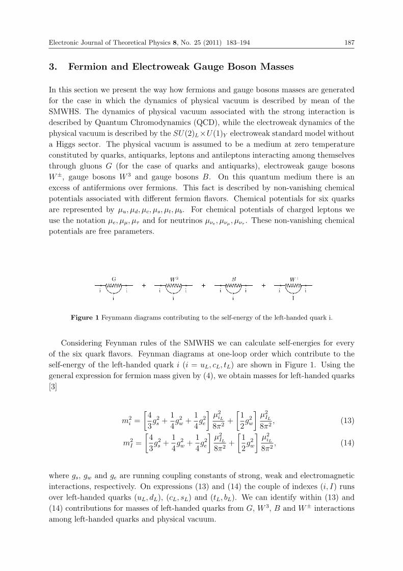
Electronic Journal of Theoretical Physics 8, No. 25 (2011) 183–194 187
3. Fermion and Electroweak Gauge Boson Masses
In this section we present the way how fermions and gauge bosons masses are generated
for the case in which the dynamics of physical vacuum is described by mean of the
SMWHS. The dynamics of physical vacuum associated with the strong interaction is
described by Quantum Chromodynamics (QCD), while the electroweak dynamics of the
physical vacuum is described by the SU(2)L×U(1)Y electroweak standard model without
a Higgs sector. The physical vacuum is assumed to be a medium at zero temperature
constituted by quarks, antiquarks, leptons and antileptons interacting among themselves
through gluons G (for the case of quarks and antiquarks), electroweak gauge bosons
W±, gauge bosons W 3 and gauge bosons B. On this quantum medium there is an
excess of antifermions over fermions. This fact is described by non-vanishing chemical
potentials associated with different fermion flavors. Chemical potentials for six quarks
are represented by μu, μd, μc, μs, μt, μb. For chemical potentials of charged leptons we
use the notation μe, μμ, μτ and for neutrinos μνe , μνμ , μντ . These non-vanishing chemical
potentials are free parameters.
Figure 1 Feynmann diagrams contributing to the self-energy of the left-handed quark i.
Considering Feynman rules of the SMWHS we can calculate self-energies for every
of the six quark flavors. Feynman diagrams at one-loop order which contribute to the
self-energy of the left-handed quark i (i = uL, cL, tL) are shown in Figure 1. Using the
general expression for fermion mass given by (4), we obtain masses for left-handed quarks
[3]
m2i =
[4
3g2s +
1
4g2w +
1
4g2e
]μ2iL
8π2+
[1
2g2w
]μ2IL
8π2, (13)
m2I =
[4
3g2s +
1
4g2w +
1
4g2e
]μ2IL
8π2+
[1
2g2w
]μ2iL
8π2, (14)
where gs, gw and ge are running coupling constants of strong, weak and electromagnetic
interactions, respectively. On expressions (13) and (14) the couple of indexes (i, I) runs
over left-handed quarks (uL, dL), (cL, sL) and (tL, bL). We can identify within (13) and
(14) contributions for masses of left-handed quarks from G, W 3, B and W± interactions
among left-handed quarks and physical vacuum.
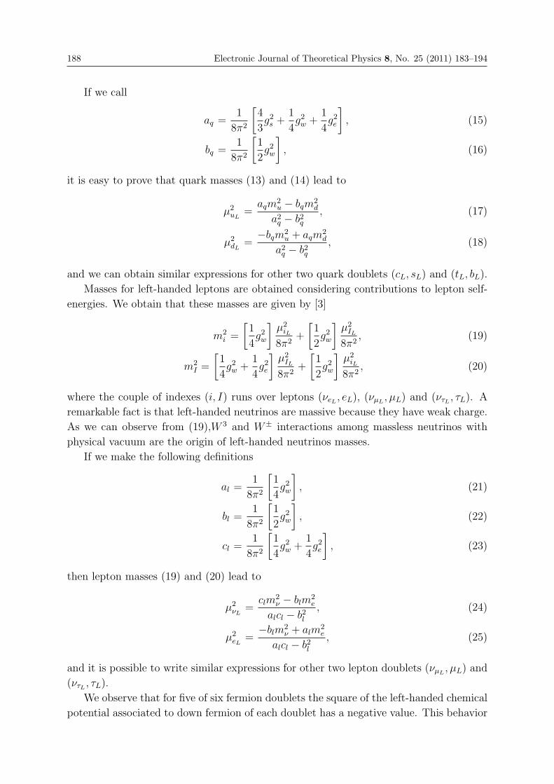
188 Electronic Journal of Theoretical Physics 8, No. 25 (2011) 183–194
If we call
aq =1
8π2
[4
3g2s +
1
4g2w +
1
4g2e
], (15)
bq =1
8π2
[1
2g2w
], (16)
it is easy to prove that quark masses (13) and (14) lead to
μ2uL
=aqm
2u − bqm
2d
a2q − b2q, (17)
μ2dL=−bqm2
u + aqm2d
a2q − b2q, (18)
and we can obtain similar expressions for other two quark doublets (cL, sL) and (tL, bL).
Masses for left-handed leptons are obtained considering contributions to lepton self-
energies. We obtain that these masses are given by [3]
m2i =
[1
4g2w
]μ2iL
8π2+
[1
2g2w
]μ2IL
8π2, (19)
m2I =
[1
4g2w +
1
4g2e
]μ2IL
8π2+
[1
2g2w
]μ2iL
8π2, (20)
where the couple of indexes (i, I) runs over leptons (νeL , eL), (νμL, μL) and (ντL , τL). A
remarkable fact is that left-handed neutrinos are massive because they have weak charge.
As we can observe from (19),W 3 and W± interactions among massless neutrinos with
physical vacuum are the origin of left-handed neutrinos masses.
If we make the following definitions
al =1
8π2
[1
4g2w
], (21)
bl =1
8π2
[1
2g2w
], (22)
cl =1
8π2
[1
4g2w +
1
4g2e
], (23)
then lepton masses (19) and (20) lead to
μ2νL=clm
2ν − blm
2e
alcl − b2l, (24)
μ2eL=−blm2
ν + alm2e
alcl − b2l, (25)
and it is possible to write similar expressions for other two lepton doublets (νμL, μL) and
(ντL , τL).
We observe that for five of six fermion doublets the square of the left-handed chemical
potential associated to down fermion of each doublet has a negative value. This behavior

Electronic Journal of Theoretical Physics 8, No. 25 (2011) 183–194 189
is observed for the case in which there is a large difference between masses of both fermions
of the same doublet. Since up and down quarks have approximately equivalent masses,
the mentioned behavior is not observed for the left-handed quark doublet formed by up
and down quarks. For this case chemical potentials associated to these two left-handed
quarks are positive.
On the other hand, applying expressions (11) and (12) for the SMWHS case, we
obtain masses for gauge bosons [3]
M2W± =
g2w2
μ2uL+ μ2
dL+ μ2
cL− μ2
sL+ μ2
tL− μ2
bL+∑3
i=1(μ2νiL− μ2
eiL)
4π2, (26)
M2W 3 =
g2w4
μ2uL+ μ2
dL+ μ2
cL− μ2
sL+ μ2
tL− μ2
bL+∑3
i=1(μ2νiL− μ2
eiL)
2π2, (27)
M2B =
g2e4
μ2uL+ μ2
dL+ μ2
cL− μ2
sL+ μ2
tL− μ2
bL+∑3
i=1(μ2νiL− μ2
eiL)
2π2, (28)
where the summation runs over the three leptons families. It is important to remember
that if the fermionic chemical potential has an imaginary value then its contribution
to the gauge boson effective mass, as in the case (11) or (12), is negative. This fact
means that finally the contribution from every fermionic left-handed chemical potential
to masses of gauge bosons is always positive.
For well known physical reasons W 3μ and Bμ gauge bosons are mixed. After diago-
nalization of the mass matrix, we get physical fields Aμ and Zμ corresponding to photon
and neutral Z0 boson of mass MZ respectively, through relations [15, 16]
M2Z =M2
W +M2B, (29)
cos θw =MW
MZ
, sin θw =MB
MZ
, (30)
where θw is the weak mixing angle
Z0μ = Bμ sin θw −W 3
μ cos θw, (31)
Aμ = Bμ cos θw +W 3μ sin θw. (32)
Substituting expressions (17), (18), (24), (25) for fermionic left-handed chemical po-
tentials into expressions (26), (27), (28) we obtain masses of electroweak gauge bosons
W and Z in terms of fermion masses and running coupling constants of strong, electro-
magnetic and weak interactions. Masses of electroweak gauge bosons can be written as
[3]
M2W = g2w(A1 + A2 + A3 − A4), (33)
M2Z = (g2e + g2w)(A1 + A2 + A3 − A4), (34)

190 Electronic Journal of Theoretical Physics 8, No. 25 (2011) 183–194
where the parameters A1, A2, A3 and A4 are
A1 =m2
u +m2d
B1
, (35)
A2 =m2
c −m2s +m2
t −m2b
B2
, (36)
A3 =3(m2
e +m2μ +m2
τ )
B3
, (37)
A4 =(3 + g2e/g
2w)(m
2νe +m2
νμ +m2ντ )
B3
, (38)
and where
B1 =4
3g2s +
3
4g2w +
1
4g2e , (39)
B2 =4
3g2s −
1
4g2w +
1
4g2e , (40)
B3 =3
4g2w −
1
4g2e . (41)
It is straight to show that if we take central experimental values for the strong
constant at the MZ scale as αs(MZ) = 0.1184, the fine-structure constant as αe =
7.2973525376×10⁻³ and the cosine of the electroweak mixing angle as cos θw =MW/MZ =
80.399/91.1876 = 0.88168786 [17], then gs = 1.21978, gw = 0.641799 and ge = 0.343457.
Substituting the values of gs, gw and ge and the values for the experimental masses of
the electrically charged fermions, given by [17] mu = 0.0025 GeV, md = 0.00495 GeV,
mc = 1.27 GeV, ms = 0.101 GeV, mt = 172.0 ± 2.2 GeV, mb = 4.19 GeV, me =
0.510998910 × 10⁻³ GeV, mμ = 0.105658367 GeV, mτ = 1.77682 GeV, into the expres-
sions (33) and (34), and assuming neutrinos as massless particles, mνe = mνμ = mντ = 0,
we obtain that theoretical masses of the W and Z electroweak gauge bosons are given by
M thW± = 79.9344± 1.0208GeV (42)
M thZ = 90.6606± 1.1587GeV . (43)
These theoretical masses are in agreement with theirs experimental values given by
M expW = 80.399 ± 0.023 GeV and M exp
Z = 91.1876 ± 0.0021 GeV [17]. Central values
for parameters A1, A2, A3 and A4 in expressions (33) and (34) are A1 = 1.32427× 10⁻⁵,A2 = 15478, A3 = 34.0137 and A4 = 0. We observe that A2 is very large respect to
A3 and A1. Taking into account the definition of parameter A2 given by (36) we can
conclude that masses of electroweak gauge bosons coming specially from top quark mass
mt and strong running coupling constant gs. Notwithstanding neutrino masses are not
known, direct experimental results show that neutrino masses are of order 1 eV [17], and
cosmological interpretations of five-year WMAP observations find a limit on the total
mass of neutrinos of Σmν < 0.6 eV (95% CL) [18]. These results assure us that values
of left-handed lepton chemical potentials obtained of taking neutrinos to be massless will
change a little if we take true small neutrinos masses.

Electronic Journal of Theoretical Physics 8, No. 25 (2011) 183–194 191
4. Some Consequences of this Approach
We note that expressions (33) and (34) establish a very close relationship among twelve
fermion masses and three interaction running coupling constants with masses of W and
Z electroweak gauge bosons. This fact let us obtain some consequences that we are
presenting next.
We conclude that expressions (33) and (34) reasons by experimental uncertainties of
electroweak gauge boson masses restrict the existence of a new family of fermions in the
SMWHS. We can arrive to this conclusion if we suppose the existence of a new fermion
family. We represent the two new leptons as νn and ln, the two new quarks as un and
dn, and the mass of these four fermions as mνn , mln , mun and mdn , respectively. We
hope that these fermion masses must be heavier than the ones of the third family. These
masses could satisfy: (i) The non-hierarchy condition given bymνn ∼ mln andmun ∼ mdn
; (ii) the hierarchy condition expressed by mνn � mln and mun � mdn . From the first
condition, expressions (33) and (34) are modified by the inclusion of terms which are
proportional to m2νn +m
2lnand m2
un+m2
dn. From the second condition, these expressions
are modified by terms which are proportional tom2νn−m2
lnand m2
un−m2
dn. Both cases are
strongly suppressed by experimental uncertainties for electroweak gauge boson masses.
On this way, our approach establishes a strong restriction for possible existence of the
fourth fermion family in the SMWHS.
We obtain also a prediction for top quark mass starting from the expression (34).
Using central experimental values for Z and W electroweak gauge boson masses and un-
certainties for running coupling constants and for fermion masses, and assuming neutrinos
as massless particles, we predict from (34) that top quark mass ismtht = 173.0015±0.6760
GeV. This theoretical value is in agreement with the experimental value for top quark
mass given by [17] mexpt = 172.0± 2.2 GeV.
If we write (38) as
A4 =(3 + g2e/g
2w)(Σm
2ν)
B3
, (44)
from (34) we obtain that for the summing of squares of neutrino masses Σm2ν can be
written as
Σm2ν =
[A1 + A2 + A3 −
M2Zmin
g2e + g2w
]B3
3 + g2e/g2w
, (45)
whereMZminis the smallest experimental value of Z mass given byMZmin
= 91.1855 GeV.
Usingmt = 173.0015 GeV and central experimental values for fermion masses and running
coupling constants that we have used in section 3, we obtain that Σm2ν = 0.06213 GeV2.
This approach for mass generation predicts that left-handed neutrinos are massive, but
this can not predict about the values for neutrino masses due to that fermionic chemical
potentials are free parameters. However we find a highest limit for the summing of squares
of neutrino masses given by Σm2ν < 0.06213 GeV2

192 Electronic Journal of Theoretical Physics 8, No. 25 (2011) 183–194
Conclusions
We have presented an approach of mass generation for Standard Model particles in which
we have extracted some generic features of the Higgs mechanism that do not depend on
its interpretation in terms of a Higgs field. On this approach the physical vacuum has
been assumed to be a medium at zero temperature which is formed by fermions and an-
tifermions interacting among themselves by exchanging gauge bosons. The fundamental
effective model describing the dynamics of this physical vacuum is the SMWHS. We have
assumed that every fermion flavor in physical vacuum has associated a chemical potential
μf in such a way that there is an excess of antifermions over fermions. This fact implies
that physical vacuum can be understood as a virtual medium having an antimatter finite
density.
Fermion masses are calculated starting from fermion self-energy which represents fun-
damental interactions of a fermion with the physical vacuum. The gauge boson masses
are calculated from the charge fluctuations of physical vacuum which are described by
a vacuum polarization tensor. Using this approach for particle mass generation we have
generated masses for the electroweak gauge bosons in agreement with their experimental
values.
A further result of this approach is that left-handed neutrinos are massive due to that
they have weak charge. Additionally our approach has established a strong restriction to
the existence of a new fermion family in the SMWHS. We have also predicted that top
quark mass is mtht = 173.0015± 0.6760 GeV. Finally we have obtained the highest limit
for the summing of squares of neutrino masses given by Σm2ν < 0.06213 GeV2
Acknowledgments
We thank Vicerrectoria de Investigaciones of Universidad Nacional de Colombia by the
financial support received through the research grant ”Teorıa de Campos Cuanticos apli-
cada a sistemas de la Fısica de Partıculas, de la Fısica de la Materia Condensada y a la
descripcion de propiedades del grafeno”. C. Quimbay thanks to Rafael Hurtado, Rodolfo
Dıaz and Antonio Sanchez for stimulating discussions.
References
[1] S. Weinberg, The quantum theory of fields. Modern Applications, Vol. II. CambridgeUniversity Press, Cambridge (1996).
[2] A. Djouadi, The Anatomy of electro-weak symmetry breaking. I: The Higgs boson inthe standard model, Phys. Rept. 457, 1-216 (2008).
[3] C. Quimbay, J. Morales, Particle mass generation from physical vacuum, Apeiron 8,161-202 (2011); Effective model for particle mass generation, ArXiv:hep-ph/0702145(2007); A new approach to generate dynamically the masses of elementary particles,Rev. Col. Fis. 34, 347-350 (2002).

Electronic Journal of Theoretical Physics 8, No. 25 (2011) 183–194 193
[4] J. Schwinger, Quantum electrodynamics. I A covariant formulation, Phys. Rev 74,1439-1461 (1948); Quantum electrodynamics. 2. Vacuum polarization and selfenergy,Phys. Rev 75, 651-679 (1949).
[5] M. Le Bellac, Thermal field theory, Cambridge monographs on mathematical physics,Cambridge University Press, Cambridge (1996).
[6] H. A. Weldon, Covariant calculations at finite temperature: The relativistic plasma,Phys. Rev. D 26, 1394-1407 (1982); Dynamical holes in the quark - gluon plasma,Phys. Rev. D 40, 2410-2420 (1989).
[7] K. Kajantie, P. V. Ruuskanen, Shielding of quark mass singularities in photonemission from hot quark - gluon plasm, Phys. Lett. B 121, 352 (1983).
[8] E. J. Levinson, D. H. Boal, Selfenergy corrections to fermions in the presence of athermal background, Phys. Rev. D 31, 3280-3284 (1985).
[9] J. P. Blaizot, J. Y. Ollitrault, Collective fermionic excitations in systems with a largechemical potential, Phys. Rev. D 48, 1390-1408 (1993).
[10] J. Morales, C. Quimbay, F. Fonseca, Fermionic dispersion relations at finitetemperature and nonvanishing chemical potentials in the minimal standard model,Nucl. Phys. B 560, 601-616 (1999); C. Quimbay, S. Vargas-Castrillon, Fermionicdispersion relations in the standard model at finite temperature, Nucl. Phys. B 451,265-304 (1995).
[11] E. Braaten, D. Segel, Neutrino energy loss from the plasma process at all temperaturesand densities, Phys. Rev. D 48, 1478-1491 (1993).
[12] T. Altherr, U. Kraemmer, Gauge field theory methods for ultra-degenerate and ultra-relativistic plasmas, Astropart. Phys. 1, 133-158 (1992).
[13] H. A. Weldon, Covariant calculations at finite temperature: The relativistic plasma,Phys. Rev. D 26, 1394-1407 (1982).
[14] M. Bluhm, B. Kampfer, Quasiparticle model of quark-gluon plasma at imaginarychemical potential, Phys. Rev. D 77, 034004 (2008).
[15] S. Weinberg, A model of leptons, Phys. Rev. Lett. 19, 1264-1266 (1967).
[16] J. Pestieau, P. Roy, Lepton symmetry and selfmass, Phys. Rev. Lett. 23, 349 (1969);Historical note on the derivation of the strength of neutral current weak interactions,Lett. Nuovo Cimento 31, 625 (1981).
[17] K. Nakamura et al. (Particle Data Group), The review of particle physics, J. Phys. G37, 075021 (2010).
[18] E. Komatsu et al., Five-year Wikinson microwave anisotropy probe (WMAP)observations: Cosmological interpretations, Astrophys. J. Suppl. 180 330 (2009);ArXiv:0803.0547 [astro-ph] (2008).


EJTP 8, No. 25 (2011) 195–210 Electronic Journal of Theoretical Physics
Quantum Mechanics as Asymptotics of Solutions ofGeneralized Kramers Equation
E. M. Beniaminov∗
Sumskaya st. 6-3-76, Moscow, 117587, Russia
Received 6 July 2010, Accepted 10 February 2011, Published 25 May 2011
Abstract: We consider the process of diffusion scattering of a wave function given on the
phase space. In this process the heat diffusion is considered only along momenta. We write
down the modified Kramers equation describing this situation. In this model, the usual quantum
description arises as asymptotics of this process for large values of resistance of the medium per
unit of mass of particle. It is shown that in this case the process passes several stages. During the
first short stage, the wave function goes to one of “stationary” values. At the second long stage,
the wave function varies in the subspace of “stationary” states according to the Schrodinger
equation. Further, dissipation of the process leads to decoherence, and any superposition of
states goes to one of eigenstates of the Hamilton operator. At the last stage, the mixed state
of heat equilibrium (the Gibbs state) arises due to the heat influence of the medium and the
random transitions among the eigenstates of the Hamilton operator. Besides that, it is shown
that, on the contrary, if the resistance of the medium per unit of mass of particle is small, then
in the considered model, the density of distribution of probability ρ = |ϕ|2 satisfies the standardLiouville equation, as in classical statistical mechanics.c© Electronic Journal of Theoretical Physics. All rights reserved.
Keywords: Quantum Mechanics; Asymptotics Solution; Kramers Equation; Diffusion Scattering
PACS (2010): 03.65.-w; 02.60.Lj; 05.70.-a;02.30.Jr
1. Description and Some Properties of the Model
As in [2], we consider certain mathematical model of a process whose state at each moment
of time is given by a wave function, which is a complex valued function ϕ(x, p), where
(x, p) ∈ R2n, on the phase space, and n is the dimension of the configuration space. In
contrast to quantum mechanics, where the wave function depends only on coordinates
or only on momenta, in our case the wave function depends both on coordinates and on
momenta. By analogy with quantum mechanics, it is assumed that wave functions obey

196 Electronic Journal of Theoretical Physics 8, No. 25 (2011) 195–210
the superposition principle, and the density of probability ρD(x, p) in a bounded domain
of the phase space (x, p) ∈ D ⊂ R2n, corresponding to the wave function ϕ(x, p), is given
by the standard formula
ρD(x, p) = |ϕ(x, p)|2/∫D
|ϕ(x, p)|2dxdp. (1)
In quantum mechanics, the time evolution of the wave function can be defined by the
Feynman path integral [3]. The Feynman principle assumes that if at the initial moment
t = t0 a wave function ϕ(x0, p0, t0) is given, then the value of the wave function at the point
(x, p) at the moment t = t1 is defined by the integral over all paths {x(t), p(t)} joiningthe points (x0, p0, t0) and (x, p, t1), of the quantity exp
(− i
�
∫ t1t0[V (x(t))− p2(t)/(2m)]dt
),
where � is the Planck constant, with respect to certain “measure” on paths defined by
Feynman.
In contrast to Feynman’s assumption, in the present paper we study the model in
which the Feynman measure on paths is replaced by the probability measure of the
diffusion process (the heat Brownian motion) given by the Kramers equation [4], [5]:
∂f
∂t=
n∑j=1
(∂V
∂xj
∂f
∂pj− pjm
∂f
∂xj
)+ γ
n∑j=1
∂
∂pj
(pjf + kTm
∂f
∂pj
), (2)
where f(x, p, t) is the density of probability distribution of the particle in the phase space
at the moment of time t; m is the mass of the particle; V (x) is the potential function
of the external forces acting on the particle; γ = β/m is the resistance coefficient of
the medium per unit of mass; k is the Boltzmann constant; T is the temperature of the
medium.
This is the classical Kramers equation describing the diffusion motion of a particle in
the phase space under action of external forces defined by the potential function V (x),
the heat medium with temperature T , and the medium resistance per unit of mass γ.
Consider the following modified Kramers equation for the wave function ϕ(x, p, t):
∂ϕ
∂t= Aϕ+ γBϕ, (3)
where Aϕ =n∑
j=1
(∂V
∂xj
∂ϕ
∂pj− pjm
∂ϕ
∂xj
)− i
�
(mc2 + V −
n∑j=1
p2j2m
)ϕ (4)
Bϕ =n∑
j=1
∂
∂pj
((pj + i�
∂
∂xj
)ϕ+ kTm
∂ϕ
∂pj
).
Equation (3) is obtained from the Kramers equation (2) by adding to the right hand side
the summand of the form −i/�(mc2 + V − p2/(2m))ϕ and by replacing multiplication of
the function ϕ by pj in the diffusion operator by the action of the operator (pj+ i�∂/∂xj)
on the function ϕ.
Adding the summand−i/�(mc2+V−p2/(2m))ϕ is related with the additional physicalrequirement that the wave function at the point (x, p) oscillates harmonically with the
frequency 1/�(mc2 + V − p2/(2m)) in time.

Electronic Journal of Theoretical Physics 8, No. 25 (2011) 195–210 197
The requirement of harmonic oscillation of the wave function ϕ at the point (x, p)
with large frequency 1/�(mc2 + V − p2/(2m)), in the case when mc2 is much greater
than V , gives that the shift of the wave function with respect to coordinate xj with
conservation of the proper time at the point (x, p) yields the phase shift in the oscillation
of the function ϕ. This also gives that the operator of infinitesimal shift ∂/∂xj is replaced
by the operator ∂/∂xj − ipj/�. (For a more detailed explanation, see [2].) Respectively,
if one multiplies this operator by i�, then one obtains the operator pj + i�∂/∂xj used in
the modified diffusion operator B.
Let us proceed to the study of equation (3).
In order to separate mathematics from physics in this equation, let us make a change
of variables and let us pass to dimensionless quantities:
t′ = γt, p′ =p√kTm
, x′ =
√kTm
�x, V ′(x) =
V (x)
kT. (5)
In the new variables equation (3) takes the following form:
∂ϕ
∂t′=kT
γ�A′ϕ+B′ϕ, (6)
where A′ϕ =n∑
j=1
(∂V ′
∂x′j
∂ϕ
∂p′j− p′j
∂ϕ
∂x′j
)− i
(mc2
kT+ V ′ −
n∑j=1
(p′j)2
2
)ϕ (7)
B′ϕ =n∑
j=1
∂
∂p′j
((p′j + i
∂
∂x′j
)ϕ+
∂ϕ
∂p′j
).
The parameter of the model described by equation (6), is the dimensionless quantity
kT/(γ�), which we denote by ε.
Let us assume that ε = kT/(γ�) is a small quantity which is the small perturbation
parameter in equation (6) with the non-perturbed equation ∂ϕ/∂t′ = B′ϕ, i. e., theequation
∂ϕ
∂t′=
n∑j=1
∂
∂p′j
((p′j + i
∂
∂x′j
)ϕ+
∂ϕ
∂p′j
). (8)
Note that the smallness of the quantity ε = kT/(γ�) requires that the friction coefficient
of the medium per unit of mass γ = β/m = (k/�)T/ε = 1.3 · 1011T/ε be greater than1.3 · 1011T , since k/� = 1.3 · 1011.
Let us substitute into equation (8) the Fourier integral presentation of ϕ(x′, p′, t′) withrespect to x′:
ϕ(x′, p′, t′) =1
(2π)n/2
∫Rn
ϕ(s′, p′, t′)eis′x′ds′, (9)
where ϕ(s′, p′, t′) =1
(2π)n/2
∫Rn
ϕ(x′, p′, t′)e−is′x′dx′. (10)
We obtain that ϕ(s′, p′, t′) satisfies the equation
∂ϕ
∂t′=
n∑j=1
∂
∂p′j
((p′j − s′j)ϕ+
∂ϕ
∂p′j
). (11)

198 Electronic Journal of Theoretical Physics 8, No. 25 (2011) 195–210
The operator of the right hand side of this equation is well known (see, for example,
[6]). This operator has a full set of eigenfunctions in the space of functions tending to
zero as |p′| tends to infinity. The eigenvalues of this operator are nonpositive integers.The eigenfunctions corresponding to the eigenvalue 0 have the form
ϕ0(s′, p′) =
1
(2π)n/2ψ(s′)e−
(p′−s′)22 ,
where ψ(s′) is an arbitrary complex valued function of s′ ∈ Rn .
The rest of eigenfunctions are obtained as derivatives of the functions ϕ0(s′, p′) with
respect to p′, and have eigenvalues −1,−2, ..., respectively, depending on the degree of
derivative, and the projector P0 to the subspace of eigenfunctions with eigenvalue 0 has
the form
ϕ0(s′, p′) = P0ϕ =
1
(2π)n/2ψ(s′)e−
(p′−s′)22 , where ψ(s′) =
∫Rn
ϕ(s′, p′)dp′. (12)
Hence, considering equation (11) in the basis of these eigenfunctions, we obtain that each
solution ϕ(s′, p′, t′) of this equation tends exponentially in time with exponent −1 to astationary solution of the form ϕ0. Therefore, taking into account the presentation (9) of
the function ϕ(x′, p′, t) via ϕ(s′, p′, t′), we obtain that “stationary” solutions ϕ0(x′, p′) of
equation (6) look as follows:
ϕ0(x′, p′) =
1
(2π)n
∫Rn
ψ(s′)e−(p′−s′)2
2 eis′x′ds′.
Let us present the function ψ(s′), in its turn, as the Fourier integral:
ψ(s′) =1
(2π)n/2
∫Rn
ψ(y′)e−is′y′dy′.
Substituting this presentation into the preceding expression and integrating over s′, weobtain
ϕ0(x′, p′) =
1
(2π)3n/2
∫R2n
ψ(y′)e−(p′−s′)2
2 eis′(x′−y′)ds′ dy′
=1
(2π)n
∫Rn
ψ(y′)e−(x′−y′)2
2 eip′(x′−y′)dy′
or, taking into account (12),
ϕ0 = P0ϕ =1
(2π)n
∫Rn
ψ(y′)e−(x′−y′)2
2 eip′(x′−y′)dy′, where ψ(y′) =
∫Rn
ϕ(y′, p′)dp′. (13)
Thus, if ε is small, then at the time t′ of order 1, a solution of equation (6), starting
from an arbitrary function ϕ, will become close to a function of the form ϕ0 which, in
the initial coordinates (5), reads:
ϕ0(x, p) =1
(2π�)n
∫Rn
ψ(y) exp
(−kTm(x− y)2
2�2
)exp
(ip(x− y)
�
)dy.

Electronic Journal of Theoretical Physics 8, No. 25 (2011) 195–210 199
Later the solution of equation (3), evolving in time, will be close to the subspace of
“stationary” functions of the form ϕ0.
Note that the “stationary” functions obtained here coincide, up to a normalizing
factor, with the “stationary” functions of Theorem 1 obtained in the work [2], if one
puts kTm/� equal to b/a, where a2 and b2 are the diffusion coefficients with respect to
coordinates and momenta in the model considered in [2]. Hence some results obtained in
[1], [2], hold true also in our case. We shall cite them without proof.
The results are obtained by the perturbation theory method up to second order, of
equation (6) ∂ϕ/∂t = εA′ϕ+B′ϕ for ε� 1, where A′ is a skew Hermitian operator and
B′ is an operator with nonpositive discrete spectrum.Note that this equation does not preserve the norm of the function ϕ, which we
normalize to obtain the distribution ρ(x, p). The corresponding equation preserving the
norm, which we actually study, reads ∂ϕ/∂t = εA′ϕ+B′ϕ+kϕ, where k = −(〈B′ϕ, ϕ〉+〈ϕ,B′ϕ〉)/(2〈ϕ, ϕ〉), but it is nonlinear.
2. The main results
Denote by H(x, p) = p2/(2m) + V (x) +mc2 the Hamilton function of the system.
Theorem 1. The motion described by equation (3), for small ε = kT/(γ�) asymp-
totically splits into rapid and slow motion.
1) After rapid motion the arbitrary wave function ϕ(x, p, 0) goes, in time of order
1/γ, to a function which after normalization has the form
ϕ0(x, p) =1
(2π�)n/2
∫Rn
ψ(y)χ(x− y)eip(x−y)/�dy, (14)
where ||ψ|| = 1 and χ(x− y) =
(kTm
π�2
)n/4
e−kTm(x−y)2/(2�2), (15)
The wave functions of the form (14) form a linear space. The elements of this subspace
are parameterized by the wave functions ψ(y) depending only on coordinates y ∈ Rn.
2) The slow motion starting from the wave function ϕ0(x, p) of the form (14) with
nonzero function ψ(y), goes inside the subspace and is parameterized by the wave function
ψ(y, t) depending on time. The function ψ(y, t) satisfies the Schrodinger equation of the
form i�∂ψ/∂t = Hψ, where
Hψ = − �2
2m
( n∑k=1
∂2ψ
∂y2k
)+ V (y)ψ +
kT
2nψ +mc2ψ. (16)
Proof of the first part of Theorem 1 is given in [2]. Proof of the second part of the
Theorem is given in Appendix 1 to the present paper.
Theorem 2. The projection operator P0 transforming an arbitrary integrable function
ϕ(x, p) on the phase space into the function of the form (14) (but without normalization),
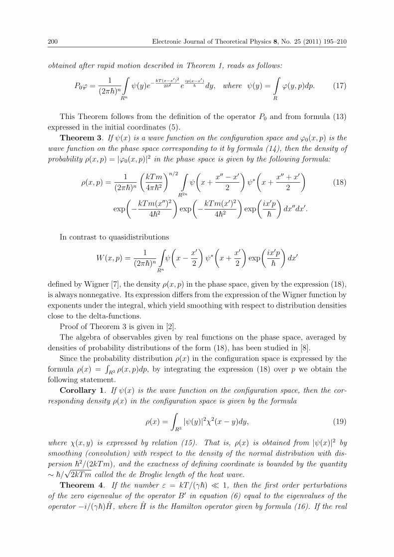
200 Electronic Journal of Theoretical Physics 8, No. 25 (2011) 195–210
obtained after rapid motion described in Theorem 1, reads as follows:
P0ϕ =1
(2π�)n
∫Rn
ψ(y)e−kT (x−x′)2
2�2 eip(x−x′)
� dy, where ψ(y) =
∫R
ϕ(y, p)dp. (17)
This Theorem follows from the definition of the operator P0 and from formula (13)
expressed in the initial coordinates (5).
Theorem 3. If ψ(x) is a wave function on the configuration space and ϕ0(x, p) is the
wave function on the phase space corresponding to it by formula (14), then the density of
probability ρ(x, p) = |ϕ0(x, p)|2 in the phase space is given by the following formula:
ρ(x, p) =1
(2π�)n
(kTm
4π�2
)n/2 ∫R2n
ψ
(x+
x′′ − x′
2
)ψ∗(x+
x′′ + x′
2
)(18)
exp
(−kTm(x
′′)2
4�2
)exp
(−kTm(x
′)2
4�2
)exp
(ix′p�
)dx′′dx′.
In contrast to quasidistributions
W (x, p) =1
(2π�)n
∫Rn
ψ
(x− x′
2
)ψ∗(x+
x′
2
)exp
(ix′p�
)dx′
defined by Wigner [7], the density ρ(x, p) in the phase space, given by the expression (18),
is always nonnegative. Its expression differs from the expression of the Wigner function by
exponents under the integral, which yield smoothing with respect to distribution densities
close to the delta-functions.
Proof of Theorem 3 is given in [2].
The algebra of observables given by real functions on the phase space, averaged by
densities of probability distributions of the form (18), has been studied in [8].
Since the probability distribution ρ(x) in the configuration space is expressed by the
formula ρ(x) =∫R3 ρ(x, p)dp, by integrating the expression (18) over p we obtain the
following statement.
Corollary 1. If ψ(x) is the wave function on the configuration space, then the cor-
responding density ρ(x) in the configuration space is given by the formula
ρ(x) =
∫R3
|ψ(y)|2χ2(x− y)dy, (19)
where χ(x, y) is expressed by relation (15). That is, ρ(x) is obtained from |ψ(x)|2 by
smoothing (convolution) with respect to the density of the normal distribution with dis-
persion �2/(2kTm), and the exactness of defining coordinate is bounded by the quantity
∼ �/√2kTm called the de Broglie length of the heat wave.
Theorem 4. If the number ε = kT/(γ�) � 1, then the first order perturbations
of the zero eigenvalue of the operator B′ in equation (6) equal to the eigenvalues of the
operator −i/(γ�)H, where H is the Hamilton operator given by formula (16). If the real

Electronic Journal of Theoretical Physics 8, No. 25 (2011) 195–210 201
parts of the second order perturbations corresponding to these first order perturbations are
different from one another, then any solution of equation (3) will go in time proportional
to 1/(γε2) = γ�2/(kT )2, to one of the eigenstates of the Hamilton operator.
Proof of the Theorem is given in Appendix 2.
This theorem describes the process called in the literature by decoherence of quan-
tum states [9], [10], [11]. The form of the estimate of the time of decoherence given in
Theorem 4, somewhat differs from the form of the estimate given in the literature, for
instance in [10]. The study of the correspondence of these estimates is the subject of
another future work.
According to Theorem 4 the process described by equation (3), in time proportional
to γ�2/(kT )2, goes to one of eigenstates of the Hamilton (energy) operator. Further, on
large scales of time the system, under the action of the heat medium, will jump from
one eigenstates to others due to large deviations of the random process. In the limit as
t→∞ the system will go to the mixed state corresponding to the heat equilibrium Gibbs
state.
We have studied equation (3) for small value of ε = kT/(γ�) and obtained that
the process described by this equation is asymptotically close to the process having the
standard quantum description. Let us now consider the same equation in the case when
the quantity ε is large.
Theorem 5. If ε = kT/(γ�) � 1, i. e. γ�/(kT ) � 1, where γ = β/m is the resis-
tance of medium per unit of mass, then the operator B in equation (3) can be neglected,
and in this case the density of probability distribution ρ(x, p, t) = ϕ(x, p, t)ϕ∗(x, p, t) sat-isfies the following classical Liouville equation:
∂ρ
∂t=
n∑j=1
(∂V
∂xj
∂ρ
∂pj− pjm
∂ρ
∂xj
). (20)
Proof of the Theorem follows from the fact that equation (3) without the operator B
is a partial differential equation of first order, consisting of sum of the Liouville operator
and the operator of multiplication by a function. The solution ϕ(x, p, t) of such equation
is obtained from the initial state ϕ(x, p) = ϕ(x, p, 0) and the characteristics x(t), p(t) of
the equation with the following initial conditions: x(0) = x, p(0) = p, in the following
form:
ϕ(x, p, t) = ϕ(x(t), p(t)) exp
(−i/�
∫ t
0
(H(x(t), p(t))− p2(t)/(2m))dt
).
Respectively, we have:
ρ(x, p, t) = ϕ(x, p, t)ϕ∗(x, p, t) = ϕ(x(t), p(t))ϕ∗(x(t), p(t)) = ρ(x(t), p(t)).
Therefore, the phase of the wave is inessential, and the density ρ(x, p, t) satisfies the
Liouville equation.
Thus, Theorem 5 states that for small value of β�/(kTm) the process described
by equation (3) is asymptotically close to the process with the classical (non-quantum)

202 Electronic Journal of Theoretical Physics 8, No. 25 (2011) 195–210
description of the motion of the particle. This case arises when the mass m of the particle
is large relative to the medium resistance β.
Conclusion
In quantum optics, one now widely uses methods of study of dynamics of quantum
processes in the phase space, see, for example, [12], where, in particular, one considers
dynamics of wave packets and interference in the phase space. On this way, one manages
to model dynamics of ions in traps, optics of atoms in quantum light fields, etc. “This
approach which stresses the fundamental role of phase variables allows one to expose and
interprete very clearly various branches of quantum optics...” (from the abstract of the
book [12]).
These achievements lead to an assumption that it would be useful to consider not
only the behavior of distributions in the phase space, as it is done, for example, in [12],
[13], [14], but also to introduce the wave function itself on the phase space.
In the present work, following this direction, we construct a diffusion equation for
the wave function with large frequency of oscillations in the phase space, describing the
process of heat scattering of a wave in the phase space. In the presented model one
meets both classical and quantum mechanics behavior of the particle. If the quantity
ε = kTm/(β�) is small, then in this model the behavior of the particle, after short
transition stage (of order m/β < �/kT = 0.77 · 10−12/T sec.) amounts to the standard
picture of quantum mechanics with the Heisenberg indeterminacy principle and with
the Schrodinger equation describing the dynamics. And if the quantity ε is large, then
the particle behaves according to classical mechanics, and the density of probability
distribution of the particle in the phase space satisfies the classical Liouville equation.
In the general case, the behavior of the particle described by this model is of mixed
nature. It would be interesting to analyze the model in this case and compare it with
results of experiments for particles with intermediate values of ε.
One should also compare with experimental data the estimate of time of decoherence
given in Theorem 4. Besides that, one should find a theoretical estimate of the transition
time of the quantum system to the mixed state of heat equilibrium in this model.
One should also acknowledge numerous works of predecessors, due to which the sub-
ject of this paper arose, the problem has been stated and the methods of its solution have
been found. This is a separate large work. In science, posing right questions gives no less
than the results obtained. Bright examples of it are the questions of A. Einstein, due to
which quantum mechanics was founded and develops up to now.
In the works of V. P. Maslov [15, 16] one has already studied certain problem of
description of motion of a distribution of charges in the phase space under action of a
random field. In [15] under certain assumptions it is proven that if the initial distribution
of charges, depending on coordinates and momenta, belongs to certain subspace, parame-
terized by complex valued functions depending on coordinates, then the distribution does
not leave this subspace, and the dynamics of such system is described by the correspond-

Electronic Journal of Theoretical Physics 8, No. 25 (2011) 195–210 203
ing Schrodinger equation. This result has certainly influenced the author while posing
the problem of the present work.
Acknowledgements
I am deeply grateful in my heart to Professor G. L. Litvinov for the many year attention
to my work, for understanding, and for help in the right organization and exposition of
the material. I am grateful to professor A. V. Stoyanovsky, who translated this paper to
English.

204 Electronic Journal of Theoretical Physics 8, No. 25 (2011) 195–210
Appendices
Appendix 1. Proof of Part 2 of Theorem 1
Consider equation (3) in the dimensionless system of variables (5). In these variables,
the equation takes the form (6), and “stationary” solutions, to which arbitrary solutions
of equation (6) tend at time t′ of order 1, have the form (13).
Let ϕ0(x′, p′, t′) be a function of the form (13) corresponding to the function ψ(y′, t′).
Let us substitute this expression into equation (6), and let us take projection of both
parts of this equation to the space of functions ψ(y′, t′) by formula (13). We have:∫Rn
∂ϕ0
∂t′dp′ =
∫Rn
(kT
γ�A′ + B′
)ϕ0dp
′
or, taking into account that B′ϕ0 = 0, after substitution of expression ϕ0(x′, p′, t′) in the
form (13), we obtain:
1
(2π)n
∫R2n
∂ψ(y′, t′)∂t′
e−(x′−y′)2
2 eip′(x′−y′)dy′dp′
=kT
γ�
1
(2π)n
∫R2n
A′ψ(y′, t′)e−(x′−y′)2
2 eip′(x′−y′)dy′dp′.
Let us integrate the right hand side of this equality over p′ and over y′. Noting that inthe right hand side of the equality we have the delta function, we obtain:
∂ψ(x′, t′)∂t′
=kT
γ�
1
(2π)n
∫R2n
A′ψ(y′, t′)e−(x′−y′)2
2 eip′(x′−y′)dy′dp′.
Taking into account expression (7) for operator A′, we deduce from the latter equality
that
∂ψ
∂t′=kT
γ�
1
(2π)n
∫R2n
(n∑
j=1
(∂V ′
∂x′j
∂
∂p′j− p′j
∂
∂x′j
)− i
(mc2
kT+ V ′ −
n∑j=1
(p′j)2
2
))
×ψ(y′, t′)e−(x′−y′)2
2 eip′(x′−y′)dy′dp′ =
kT
γ�(I1 + I2 + I3 + I4), (21)
where
I1 =1
(2π)n
∫R2n
n∑j=1
∂V ′(x′)∂x′j
∂
∂p′j
(ψ(y′, t′)e−
(x′−y′)22 eip
′(x′−y′))dy′dp′; (22)
I2 = −1
(2π)n
∫R2n
n∑j=1
p′j∂
∂x′j
(ψ(y′, t′)e−
(x′−y′)22 eip
′(x′−y′))dy′dp′; (23)
I3 = −i1
(2π)n
∫R2n
(mc2
kT+ V ′(x′)
)ψ(y′, t′)e−
(x′−y′)22 eip
′(x′−y′)dy′dp′; (24)
I4 = i1
(2π)n
∫R2n
n∑j=1
(p′j)2
2ψ(y′, t′)e−
(x′−y′)22 eip
′(x′−y′)dy′dp′. (25)

Electronic Journal of Theoretical Physics 8, No. 25 (2011) 195–210 205
Consider the integral I1 given by expression (22). Let us exchange summation and
integration, let us put behind the sign of integral expressions not depending on integration
variables, let us compute the derivatives with respect to p′j, and let us integrate the
remaining integrals over p′ and y′. We obtain:
I1 =i
(2π)n
n∑j=1
∂V ′(x′)∂x′j
∫R2n
ψ(y′, t′)e−(x′−y′)2
2 (x′j − y′j)eip′(x′−y′)dy′dp′ = 0 (26)
Consider the integral I2 given by expression (23). Let us exchange summation and
integration, let us transfer the derivatives with respect to x′j behind the sign of integral,let us replace the expressions p′j exp(ip
′(x′ − y′)) by equal expressions i∂ exp(ip′(x′ −y′))/(∂y′j), and let us integrate the obtained integrals by parts. We have:
I2 = −1
(2π)n
n∑j=1
∂
∂x′j
∫R2n
ψ(y′, t′)e−(x′−y′)2
2 i∂
∂y′jeip
′(x′−y′)dy′dp′
=i
(2π)n
n∑j=1
∂
∂x′j
∫R2n
∂ψ(y′, t′)∂y′j
e−(x′−y′)2
2 eip′(x′−y′)dy′dp′
− i
(2π)n
n∑j=1
∂
∂x′j
∫R2n
ψ(y′, t′)(x′j − y′j)e− (x′−y′)2
2 eip′(x′−y′)dy′dp′
= i
n∑j=1
∂2ψ(x′, t′)∂(x′j)2
. (27)
Consider the integral I3 given by expression (24). Let us transfer behind the sign of
integral the expressions not depending on the integration variables, and let us integrate
the remaining integral over p′ and y′. We obtain:
I3 = −i(mc2
kT+ V ′(x′)
)1
(2π)n
∫R2n
ψ(y′, t′)e−(x′−y′)2
2 eip′(x′−y′)dy′dp′
= −i(mc2
kT+ V ′(x′)
)ψ(x′, t′). (28)
Consider the integral I4 given by expression (25). Let us exchange summation and
integration, let us transfer 1/2 behind the sign of integral, let us replace the expression
(p′j)2 exp(ip′(x′ − y′)) by the second derivative of the function − exp(ip′(x′ − y′)) with

206 Electronic Journal of Theoretical Physics 8, No. 25 (2011) 195–210
respect to y′j, and let us integrate the obtained integrals by parts. We have:
I4 = −i
2
1
(2π)n
n∑j=1
∫R2n
ψ(y′, t′)e−(x′−y′)2
2∂2
∂(y′j)2eip
′(x′−y′)dy′dp′
= − i2
1
(2π)n
n∑j=1
∫R2n
(∂2ψ
∂(y′j)2− 2
∂ψ
∂y′j(x′j − y′j) + ψ(x′j − y′j)
2 + ψ
)×e−
(x′−y′)22 eip
′(x′−y′)dy′dp′
= − i2
(n∑
j=1
∂2ψ(x′, t′)∂(x′j)2
+ nψ(x′, t′)
). (29)
Let us substitute the obtained expressions for integrals I1, . . . , I4 into equality (21),
let us sum up similar terms, and let us transfer −i behind the brackets. We obtain,
∂ψ
∂t′= − i
�
kT
γ
(−12
∂2
∂(x′j)2+ V ′ +
mc2
kT+n
2
)ψ(x′, t′).
If in the obtained equality we pass to the initial coordinate system (5), then we obtain
the equality (16) required in Part 2 of Theorem 1.

Electronic Journal of Theoretical Physics 8, No. 25 (2011) 195–210 207
Appendix 2. Proof of Theorem 4
Consider equation (6) of the form ∂ϕ/∂t′ = εA′ϕ + B′ϕ. Let P0 be the projector onto
the subspace of eigenfunctions of operator B′ with eigenvalue 0. Then, by definition ofP0, we have the equalities:
P0P0 = P0; P0B′ = B′P0 = 0.
We shall denote by ϕ0 a function belonging to the image of projector P0, i. e. ϕ0 = P0ϕ0.
Note that by construction of operator H from Theorem 1, given in Appendix 1, the
operator εP0A′ on the subspace of functions ϕ0, in the presentation by the functions
ψ(y) has the form −i/(γ�)H. Hence the eigenvalues of operators εP0A′ and −i/(γ�)H
coincide. Since the operator H is self-adjoint, it has a complete system of eigenfunctions,
and therefore the operator εP0A′ on the subspace of values of the projector P0 also has
a complete system of eigenfunctions.
Let us state the result thus obtained as a Lemma.
Lemma. The eigenvalues of operators εP0A′ and −i/(γ�)H coincide. The operator
εP0A′ has a complete system of eigenfunctions on the subspace of values of the projector
P0.
Consider the eigenvalue problem for equation (6) of the form λεϕε = (εA′ + B′)ϕε.
According to perturbation theory, let us look for solutions as series:
λε = λ0 + ελ1 + ε2λ2 + ...
ϕε = ϕ0 + εϕ1 + ε2ϕ2 + ...
Let us substitute these series into the eigenvalue equation and compare coefficients before
equal powers of ε. We obtain:
(ε0) λ0ϕ0 = B′ϕ0;
(ε1) λ1ϕ0 + λ0ϕ1 = A′ϕ0 +B′ϕ1;
We are interested in perturbations of eigenvalue λ0 = 0. In this case equation (ε0)
means that ϕ0 is an eigenfunction of operator B′ with eigenvalue 0.
Let us apply the operator εP0 to both parts of equality (ε1). Taking into account the
equalities P0ϕ0 = ϕ0, λ0 = 0, and P0B′ = 0, we obtain:
ελ1ϕ0 = εP0A′ϕ0.
Hence the quantity ελ1 is an eigenvalue of the operator εP0A′ on the subspace of
values of the projector P0, and by the Lemma the quantity ελ1 is an eigenvalue of the
operator −i/(γ�)H. On the other hand, the quantity ελ1 is by definition a first order
correction to the eigenvalue 0 of the operator εA′ +B′.Thus, the first part of Theorem 4 is proved.

208 Electronic Journal of Theoretical Physics 8, No. 25 (2011) 195–210
To prove the second part, let us present an arbitrary function ϕ0(t′) from the subspace
of values of the projector P0 as a sum (or integral for continuous spectrum):
ϕ0(t′) =
∞∑k=1
ck(t′)ϕk
0,
where ϕk0 are the eigenfunctions of the operator P0A
′ with eigenvalues λk1. This is possible,since by the Lemma such functions form a complete system. Besides that, the same
Lemma implies that the numbers λk1 are pure imaginary, since they are eigenvalues of the
operator −i/(εγ�)H, where H is a self adjoint Hamilton operator with real spectrum.
Let λkε ≈ ελk1 + ε2λk2, and ϕkε ≈ ϕk
0 + εϕk1 be the approximations of eigenvalues
and eigenfunctions corresponding to eigenfunctions ϕk0. By assumptions of Theorem 4
the real parts Reλk2 are different for various k.
Consider equation (6) restricted to the subspace spanned by the basis vectors of the
form ϕkε with the function of the form
ϕ(t′) =∞∑k=1
ck(t′)ϕk
ε .
In this basis the equation splits (up to terms of order ε3) into a system of equations
numbered by k of the form:
∂ck(t′)
∂t′= (ελk1 + ε2λk2)ck(t
′),
whose solution reads as follows: ck(t′) = ck(0) exp((ελ
k1 + ε2λk2)t
′). Hence, the solution ofequation (6) is approximately presented in the following form:
ϕ(t′)=∞∑k=1
ck(0) exp((ελk1 + ε2λk2)t
′)ϕkε
=∞∑k=1
ck(0) exp((ελk1 + ε2λk2)t
′)(ϕk0 + εϕk
1)
=∞∑k=1
ck(0) exp((ελk1 + ε2λk2)t
′)ϕk0 +
∞∑k=1
ck(0) exp((ελk1 + ε2λk2)t
′)εϕk1
=ϕ0(t′) + εϕ1(t
′), (30)
where ϕ0(t′) =
∞∑k=1
ck(0) exp((ελk1 + ε2λk2)t
′)ϕk0; (31)
ϕ1(t′) =
∞∑k=1
ck(0) exp((ελk1 + ε2λk2)t
′)ϕk1. (32)
Since ε is small, equality (30) implies that the solution ϕ(t′) has a small differencewith the function ϕ0(t
′) given by expression (31).

Electronic Journal of Theoretical Physics 8, No. 25 (2011) 195–210 209
Since ελk1 is imaginary, each summand in the sum giving the function ϕ0(t′) in ex-
pression (31), decreases in time t′ = γt proportionally to
exp(ε2Re(λk2)t′) = exp(γε2Re(λk2)t),
where Re(λk2) is the real part of the number λk2. This implies that after the time t ∼
1/(γε2) this sum will be determined by the summand with the maximal number Re(λk2)
among the summands with the valuable coefficients ck(0).
Thus, Theorem 4 is proved.
References
[1] Beniaminov E. M. Diffusion processes in phase spaces and quantum mechanics //Doklady Mathematics (Proceedings of the Russian Academy of Sciences), 2007,vol.76, No. 2, 771–774.
[2] Beniaminov E. M. Quantization as asymptotics of a diffusion process in phase space//http://beniaminov.rsuh.ru/ExpandedDAN.pdf (in Russian; English translation:http://arXiv.org/abs/0812.5116v1). (2008)
[3] Feynman R., Hibbs A. Quantum mechanics and path integrals, New York: McGraw-Hill, 1965.
[4] Kramers H.A. // Physica. 1940. Vol. 7. P. 284-304.
[5] Van Kampen N.G. Stochastic Processes in Physics and Chemistry. North Holland,Amsterdam, 1981.
[6] Kamke E., Differentialgleichungen: Losungsmethoden und Losungen, I, GewohnlicheDifferentialgleichungen, B. G. Teubner, Leipzig, 1977.
[7] Wigner E. On the Quantum Correction For Thermodynamic Equilibrium // Phys.Rev. 1932. V. 40. P. 749-759.
[8] Beniaminov E.M. A Method for Justification of the View of Observables in QuantumMechanics and Probability Distributions in Phase Space http://arxiv.org/abs/quant-ph/0106112 (2001).
[9] Zeh H.D. Roots and Fruits of Decoherence. // In: Quantum Decoherence, Duplantier,B., Raimond, J.-M., and Rivasseau, V., edts. (Birkhauser, 2006), p. 151-175(arXiv:quant-ph/0512078v2).
[10] Zurek W. H. Decoherence and the transition from quantum to classical - REVISITEDarXiv:quant-ph/0306072v1. 2003 (An updated version of PHYSICS TODAY, 44:36-44 (1991)).
[11] Menskij M. B. Dissipation and decoherence of quantum systems. Physics-Uspekhi(Advances in Physical Sciences), 2003, vol.173, 1199-1219.
[12] Shlyajh V. P. Quantum optics in the phase space, Fizmatlit, Moscow, 2005. 760 pp.(in Russian).
[13] Ibort A., Man’ko V.I., Marmo G., Simoni A., Ventriglia F. On the TomographicPicture of Quantum Mechanics. Phys.Lett.A374:2614-2617, 2010. arXiv:1004.0102v1.

210 Electronic Journal of Theoretical Physics 8, No. 25 (2011) 195–210
[14] Khrennikov A. Quantum Randomness as a Result of Random Fluctuations at thePlanck Time Scale? Int. J. Theor. Phys. 2008. 47, N 1, P.114-124. arXiv:hep-th/0604011v3.
[15] Maslov V. P. Kolmogorov–Feller equations and the probabilistic model of quantummechanics. // Itogi nauki i tehniki. Probability, Mathematical Statistics andCybernetics, 1982, vol. 19, p. 55–85 (in Russian).
[16] Maslov V. P. Quantization of thermodynamics and ultrasecondary quantization,Moscow: Institute for Computer Studies, 2001, 384 pp. (in Russian).

EJTP 8, No. 25 (2011) 211–216 Electronic Journal of Theoretical Physics
Application of SU(1,1) Lie algebra in connectionwith Bound States of Poschl-Teller Potential
Subha Gaurab Roy∗1, Raghunandan Das2, Joydeep Choudhury1, NirmalKumar Sarkar3 and Ramendu Bhattacharjee1
1Department of Physics, Assam University, Silchar - 788011, India2Department of physics, Govt. Degree College, Dharmanagar -799251, India
3Department of Physics, Karimganj College, Karimganj - 788710, India
Received 23 November 2010, Accepted 10 February 2011, Published 25 May 2011
Abstract: Exactly solvable quantum mechanical potentials have attracted much attention
since the early days of quantum mechanics and the Schrodinger equation has been solved for
a large number of potentials by employing a variety of methods. Here we consider a specific
realization of SU(1,1) algebra and use it to describe the bound states of Poschl-Teller potential
without solving the Schrodinger equation for the mentioned potential.c© Electronic Journal of Theoretical Physics. All rights reserved.
Keywords: Schrodinger equation, SU(1,1) Lie algebra
PACS (2010): 31.15.xh; 03.65.Fd; 02.20.-a
1. Introduction
Group theory has wide applications in physics. The dynamical groups and their related
algebras are useful in generating the spectra and reducing the calculation of certain
transition matrix elements to algebraic manipulations. In last few years Lie algebraic
techniques have been used extensively to depict the spectra of various physical systems,
such as collective states in nuclei [1] and rotation vibration spectra in molecules. [2-8].
These applications were restricted to bound states. In all these applications, the groups
used were compact, so that their unitary representations could reproduce the observed
discrete and finite dimensional spectra. The algebras associated with the group were
used to generate the spectra [9, 10]. However, many of these systems have both discrete
and continuous spectra. For example, diatomic molecules may dissociate, above certain
energy, in two parts or one may wish to study atom-atom scattering.
∗ subha [email protected]

212 Electronic Journal of Theoretical Physics 8, No. 25 (2011) 211–216
Lie algebraic techniques based on SU(1,1) group structure could potentially be very
useful in describing bound state problems as that based on SU(2) group. The group
structure associated with the bound state problem is generally that of SU(2). The group
SU(2) can be realized either on a two dimensional harmonic oscillator space or on a sphere.
The first realization is connected with the Morse potential [11]. The second realization is
connected with the Poschl Teller potential [12]. This Poschl Teller potential emerges in
a variety of problems in physics, such as the soliton solutions to the Korteweg-de Vries
equation [13], the Hartree mean field equation of a many-body system with a δ-function
two-body interaction [14] and in connection with completely integrable many-body one-
dimensional systems [15]. Also how several potentials can be generated by SU(1,1) are
described by C. V. Sukumar and G. Levai [16].
In all the earlier works [11-16] bound and scattering states were described separately
i.e. SU(2) algebra was used to describe the bound states while SU(1,1) was used to
describe the scattering states only. But no works has been reported yet to describe the
bound states of a potential with the help of SU(1,1) algebra. So in this paper we aim to
describe how one can get hold of the bound states of Poschl-Teller potential employing the
algebra of only SU(1,1) group without following the traditional SU(2) algebraic approach
or without solving the Schrodinger equation.
2. Mathematical Calculations
To start with we reproduce a construction of the Lie group SU(1,1) generated by three
(angular momentum) operators Jx, Jy, Jz which obey SU(1,1) Lie algebraic commutation
relations as they satisfy the following commutation relations
[Jx, Jy] = −iJz, [Jy, Jz] = iJx, [Jz, Jx] = iJy
Now as the algebra is SU(1,1), so the Casimir operator (C) can be written as
C = J2 = J2z − J2
x − J2y = Jz(Jz − 1)− J−J+ (1)
where the operators J+and J−are defined as J± = Jx ± JyAlso this algebra has the realization
Jx = − i [y∂z + z∂y]
Jy = i [x∂z + z∂x] and
Jz = − i [x∂y − y∂x]
Also the simultaneous eigen states of J2 and Jz can be written as
J2 |j,m〉 = j (j + 1) |j,m〉
Jz |j,m〉 = m |j,m〉
⎤⎥⎦ (2)
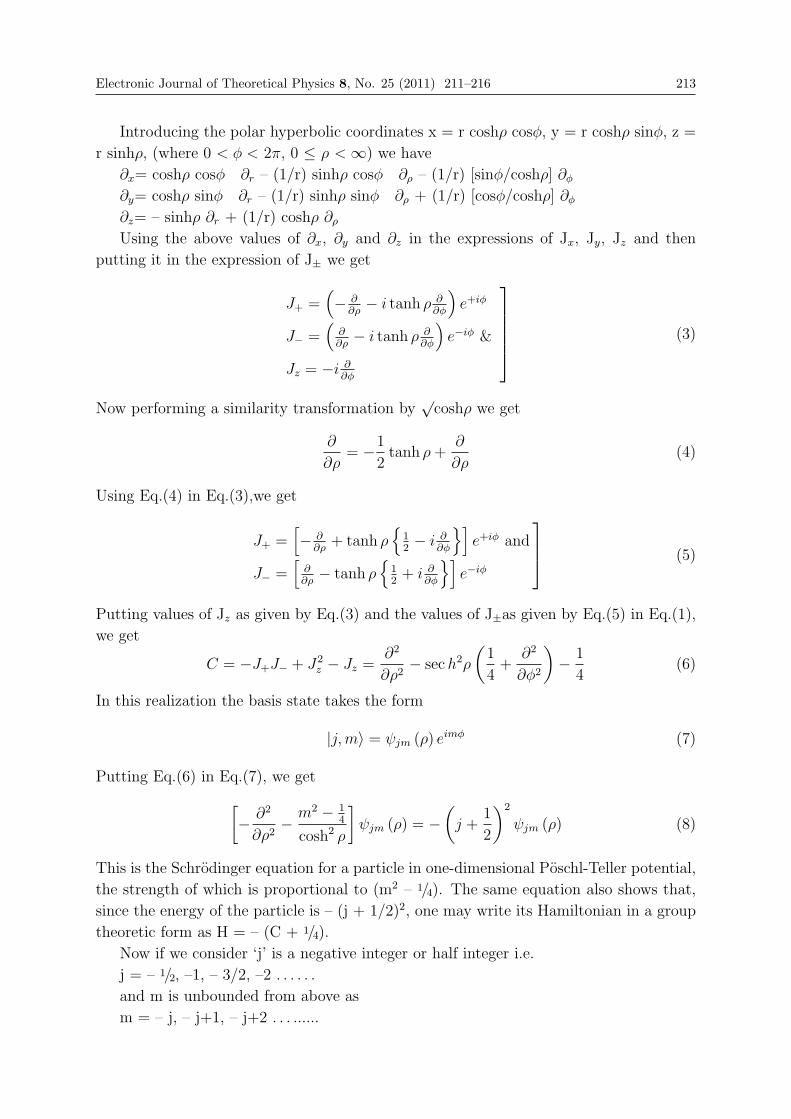
Electronic Journal of Theoretical Physics 8, No. 25 (2011) 211–216 213
Introducing the polar hyperbolic coordinates x = r coshρ cosφ, y = r coshρ sinφ, z =
r sinhρ, (where 0 < φ < 2π, 0 ≤ ρ <∞) we have
∂x= coshρ cosφ ∂r – (1/r) sinhρ cosφ ∂ρ – (1/r) [sinφ/coshρ] ∂φ∂y= coshρ sinφ ∂r – (1/r) sinhρ sinφ ∂ρ + (1/r) [cosφ/coshρ] ∂φ∂z= – sinhρ ∂r + (1/r) coshρ ∂ρUsing the above values of ∂x, ∂y and ∂z in the expressions of Jx, Jy, Jz and then
putting it in the expression of J± we get
J+ =(− ∂
∂ρ− i tanh ρ ∂
∂φ
)e+iφ
J− =(
∂∂ρ− i tanh ρ ∂
∂φ
)e−iφ &
Jz = −i ∂∂φ
⎤⎥⎥⎥⎥⎦ (3)
Now performing a similarity transformation by√coshρ we get
∂
∂ρ= −1
2tanh ρ+
∂
∂ρ(4)
Using Eq.(4) in Eq.(3),we get
J+ =[− ∂
∂ρ+ tanh ρ
{12− i ∂
∂φ
}]e+iφ and
J− =[
∂∂ρ− tanh ρ
{12+ i ∂
∂φ
}]e−iφ
⎤⎥⎦ (5)
Putting values of Jz as given by Eq.(3) and the values of J±as given by Eq.(5) in Eq.(1),we get
C = −J+J− + J2z − Jz =
∂2
∂ρ2− sech2ρ
(1
4+
∂2
∂φ2
)− 1
4(6)
In this realization the basis state takes the form
|j,m〉 = ψjm (ρ) eimφ (7)
Putting Eq.(6) in Eq.(7), we get[− ∂2
∂ρ2−m2 − 1
4
cosh2 ρ
]ψjm (ρ) = −
(j +
1
2
)2
ψjm (ρ) (8)
This is the Schrodinger equation for a particle in one-dimensional Poschl-Teller potential,
the strength of which is proportional to (m2 – 1/4). The same equation also shows that,
since the energy of the particle is – (j + 1/2)2, one may write its Hamiltonian in a group
theoretic form as H = – (C + 1/4).
Now if we consider ‘j’ is a negative integer or half integer i.e.
j = – 1/2, –1, – 3/2, –2 . . . . . .
and m is unbounded from above as
m = – j, – j+1, – j+2 . . . ......

214 Electronic Journal of Theoretical Physics 8, No. 25 (2011) 211–216
Then the basis states correspond to bound states of the Poschl-Teller potential. For
a given potential (i.e., m fixed positive integer or half-integer) the bound state spectrum
is given by Ej = – (j+ 1/2)2.
On the other hand if we consider ‘j’ is a negative integer or half integer i.e.
j = – 1/2, –1, – 3/2, –2 . . . . . . . . . . . .
and m is unbounded as
m = j, j–1, j–2 . . . . . . .. . . . . . .
Then also it describes the same physical state (bound state) as the potential retains
the same symmetry as that before.
Conclusion
In this work the bound state of Poschl-Teller potential are described using a new realiza-
tion of the SU(1,1) algebra. This approach has the advantage that it can be generalised
to cases where the Hamiltonian is specified in terms of the generators of the group rather
than as a differential Schrodinger operator. Here the energy spectrum is obtained without
solving the Schrodinger equation. Also in all earlier works, SU(2) algebra was used to
describe the bound states but her we have shown that how one can explain the bound
state employing the algebra of only SU(1,1) group.
Acknowledgement
We would like to thank Mr. Pritibhajan Byakti, Dr. Uday Shankar Chakraborty, Dr.
Himadri Sekhar Das, Dr. B. I. Sharma, Dr. Sudip Choudhury and Mr. Saurav Shome for
their useful discussions and support. Subha Gaurab Roy is thankful to Assam University,
Silchar for the grant of UGC Ph.D. fellowship. Subha Gaurab Roy is also extremely
grateful to DST, New Delhi for the grant of INSPIRE fellowship.
References
[1] A. Arima and F. Iachello, Ann. Phys., 99, 253 (1976); 111, 201 (1978), and 123, 581(1981).
[2] F. Iachello, Chem. Phys. Lett., 78, 581 (1981); F. Iachello and R. D. Levine, J. Chem.Phys., 77, 4046 (1982), and O. S. van Roosmalen, A. E. L. Dieperink and F. Iachello,Chem. Phys. Lett., 85, 32 (1982).
[3] N. K. Sarkar, J. Choudhury and R. Bhattacharjee, Mol. Phys., 104, 3051 (2006);106, 693-702(2008), and Indian J. Phys., 82, 767 (2008).
[4] S. R. Karumuri, N. K. Sarkar, J. Choudhury and R. Bhattacharjee, Mol. Phys., 106,1733 (2009).
[5] J. Choudhury, S. R. Karumuri, N. K. Sarkar and R. Bhattacharjee, Pramana J.Phys., 71(3), 439 (2008); 73(5), 881 (2009); 72(3), 517 (2008) and 74, 57 (2010).

Electronic Journal of Theoretical Physics 8, No. 25 (2011) 211–216 215
[6] S. R. Karumuri, J. Choudhury, N. K. Sarkar & R. Bhattacharjee, J. EnvironmentalResearch and Development, 03, 250 (2008).
[7] J. Choudhury, N. K. Sarkar and R. Bhattacharjee, Indian J. Phys., 82, 561 (2008).
[8] J. Choudhury, S. R. Karumuri, N. K. Sarkar and R. Bhattacharjee, Chin. Phys. Lett.,26 (2), 020308-1 (2009), and 26 (9), 093301-1 (2009).
[9] Y. Alhassid and R. D. Levine, Phys. Rev. A., 18, 89 (1978).
[10] R. D. Levine and C. E. Wulfman, Chem. Phys. Lett., 60, 372 (1979).
[11] P. M. Morse, Phys. Rev., 34, 57 (1929).
[12] Y. Alhassid, F. Gursey and F. Iachello, Phys. Rev. Lett., 50, 873 (1983);
[13] S. G. Roy, J. Choudhury, N. K. Sarkar, S. R. Karumuri and R. Bhattacharjee,Electronic Journal of Theoretical Physics, 7 (24), 235-240 (2010).
[14] P. Lax, Commun. Pure Appl. Math., 27, 97 (1968).
[15] F. Calogero and A. Degasperis, Phys. Rev. A., 11, 265 (1975), and B. Yoon and J.W. Negele, Phys. Rev. A., 16, 1451 (1977).
[16] F. Calogero, Lett. Nuovo Citn., 13, 411 (1975).
[17] C. V. Sukumar, J. Phys. A: Math. Gen., 19, 2229 (1986), and G. Levai, J. Phys. A:Math. Gen., 27, 3809 (1994).

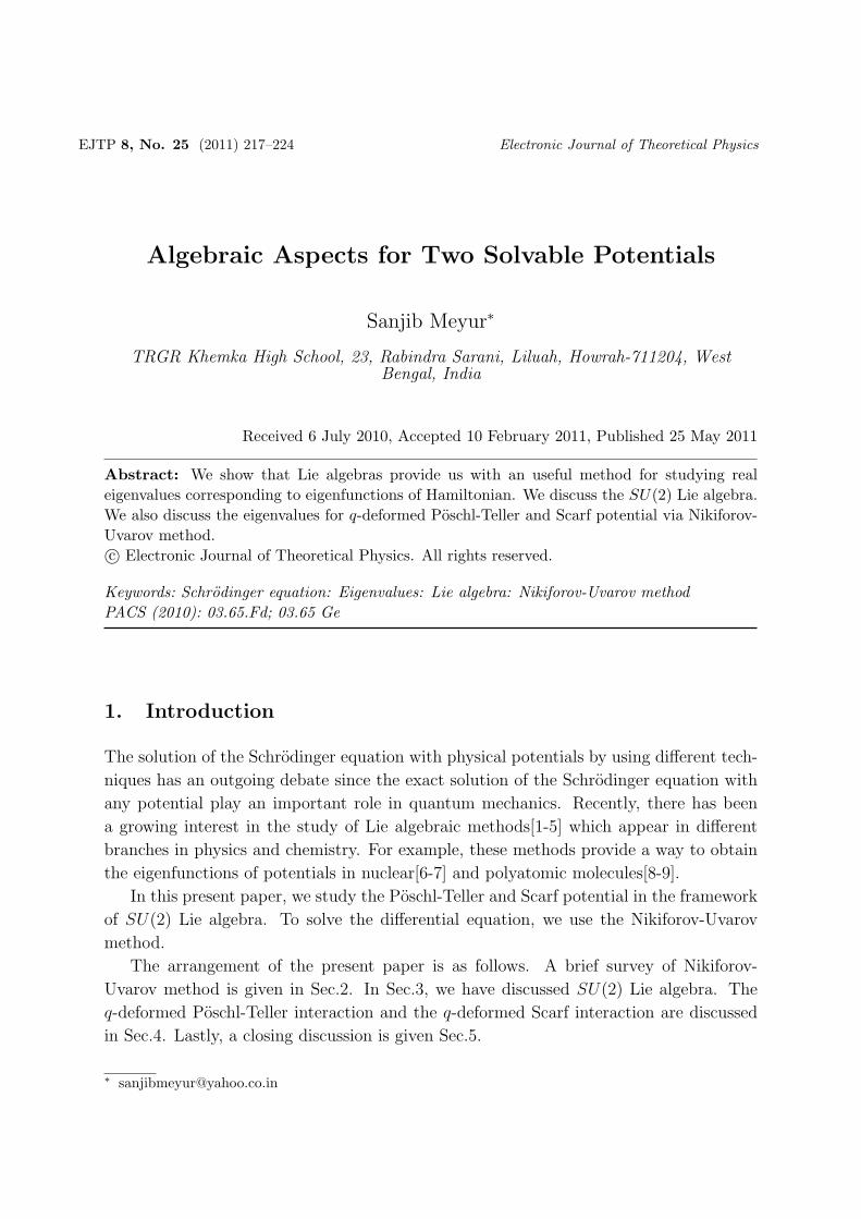
EJTP 8, No. 25 (2011) 217–224 Electronic Journal of Theoretical Physics
Algebraic Aspects for Two Solvable Potentials
Sanjib Meyur∗
TRGR Khemka High School, 23, Rabindra Sarani, Liluah, Howrah-711204, WestBengal, India
Received 6 July 2010, Accepted 10 February 2011, Published 25 May 2011
Abstract: We show that Lie algebras provide us with an useful method for studying real
eigenvalues corresponding to eigenfunctions of Hamiltonian. We discuss the SU(2) Lie algebra.
We also discuss the eigenvalues for q-deformed Poschl-Teller and Scarf potential via Nikiforov-
Uvarov method.c© Electronic Journal of Theoretical Physics. All rights reserved.
Keywords: Schrodinger equation: Eigenvalues: Lie algebra: Nikiforov-Uvarov method
PACS (2010): 03.65.Fd; 03.65 Ge
1. Introduction
The solution of the Schrodinger equation with physical potentials by using different tech-
niques has an outgoing debate since the exact solution of the Schrodinger equation with
any potential play an important role in quantum mechanics. Recently, there has been
a growing interest in the study of Lie algebraic methods[1-5] which appear in different
branches in physics and chemistry. For example, these methods provide a way to obtain
the eigenfunctions of potentials in nuclear[6-7] and polyatomic molecules[8-9].
In this present paper, we study the Poschl-Teller and Scarf potential in the framework
of SU(2) Lie algebra. To solve the differential equation, we use the Nikiforov-Uvarov
method.
The arrangement of the present paper is as follows. A brief survey of Nikiforov-
Uvarov method is given in Sec.2. In Sec.3, we have discussed SU(2) Lie algebra. The
q-deformed Poschl-Teller interaction and the q-deformed Scarf interaction are discussed
in Sec.4. Lastly, a closing discussion is given Sec.5.

218 Electronic Journal of Theoretical Physics 8, No. 25 (2011) 217–224
2. Nikiforov-Uvarov method
The conventional Nikiforov-Uvarov method[10], which received much interest, has been
introduced for solving Schrodinger equation, Klein-Gordon and Dirac equations.
The differential equations whose solutions are the special functions of hypergeometric
type can be solved by using the Nikiforov-Uvarov method which has been developed by
Nikiforov and Uvarov[10]. In this method, the one dimensional Schrodinger equation is
reduced to an equation by an appropriate coordinate transformation x = x(s),
d2ψ(s)
ds2+τ(s)
σ(s)
dψ(s)
ds+
σ(s)
σ2(s)ψ(s) = 0 (1)
where σ(s) and σ(s) are polynomials, at most of second degree, and τ(s) is a polynomial,
at most of first degree. In order to obtain a particular solution to Eq.(1), we set the
following wave function as a multiple of two independent parts
ψ(s) = φ(s)y(s) (2)
According to Eq.(1) and Eq.(2) we have
σ(s)y′′(s) + τ(s)y′(s) + λy(s) = 0 (3)
which demands that the following conditions be satisfied:
φ′(s)φ(s)
=π(s)
σ(s)(4)
τ(s) = τ(s) + 2π(s), τ ′(s) < 0 (5)
The condition τ ′(s) < 0 helps to generate energy eigenvalues and corresponding eigen-
functions. The condition τ ′(s) > 0 has widely discussed in[11] . The λ in (3) satisfies the
following second-order differential equation
λ = λn = −nτ ′(s)−n(n− 1)
2σ′′(s), n = 0, 1, 2, ....... (6)
The polynomial τ(s) with the parameter s and prime factors show the differentials at
first degree be negative. It is to be noted that λ or λn are obtained from a particular
solution of the form y(s) = yn(s) which is a polynomial of degree n. The second part
yn(s) of the wavefunction Eq.(2) is the hypergeometric-type function whose polynomial
solutions are connected by Rodrigues relation[12-14]
yn(s) =Cn
ρ(s)
dn
dsn[σn(s)ρ(s)] (7)
where Cn is normalization constant and the weight function ρ(s) satisfies the relation as
d
ds[σ(s)ρ(s)] = τ(s)ρ(s) (8)

Electronic Journal of Theoretical Physics 8, No. 25 (2011) 217–224 219
On the other hand, in order to find the eigenfunctions, φn(s) and yn(s) in Eqs.(4) and
(7) and eigenvalues λn in Eq.(6), we need to calculate the functions:
π(s) =
(σ′ − τ
2
)±
√(σ′ − τ
2
)2
− σ + kσ (9)
k = λ− π′(s) (10)
In principle, since π(s) has to be a polynomial of degree at most one, the expression under
the square root sign in Eq.(9) can be put into order to be the square of a polynomial of
first degree[10], which is possible only if its discriminant is zero. Thus, the equation for k
obtained from the solution of Eq.(9) can be further substituted in Eq.(10). In addition,
the energy eigenvalues are obtained from Eqs.(6) and (10).
3. SU(2) Lie Algebra
The generators Jx, Jy, Jz of the SU(2) group characterized by the commutation relations
[Jx, Jy] = i�Jz, [Jy, Jz] = i�Jx, [Jz, Jx] = i�Jy (11)
The differential realization in spherical coordinate (r, θ, φ) of the SU(2) generators are
Jz = −i�∂
∂φ, J2 = −�2
[1
sin θ
∂
∂θ
(sin θ
∂
∂θ
)+
1
sin2 θ
∂2
∂φ2
](12)
where 0 ≤ φ < 2π and −→J = −→r ×−→p (13)
We consider the Hamiltonian as H = −J2z and the Casimir operator corresponding to
the above generators is C = J2. The Schrodinger equation is
Cψ = J2ψ = j(j + 1)ψ (14)
Using Eqs.(11) and (14), we have[1
sin θ
∂
∂θ
(sin θ
∂
∂θ
)+
1
sin2 θ
∂2
∂φ2+ ε
]ψ = 0 (15)
where
ε =j(j + 1)
�2(16)
To solve the Eq. (15), we separated ψ(θ, φ) as
ψ(θ, φ) = Θ(θ)Φ(φ) (17)
From Eq.(15) and Eq.(17), we have two second order differential equations
d2Θ(θ)
dθ2+ cot θ
dΘ(θ)
dθ+
[ε− μ2
sin2 θ
]Θ(θ) = 0 (18)

220 Electronic Journal of Theoretical Physics 8, No. 25 (2011) 217–224
d2Φ(φ)
dφ2+ μ2Φ(φ) = 0 (19)
where μ is constant. The solution of the Eq.(19) is periodic and must satisfy the periodic
boundary condition Φ(φ+ 2π) = Φ(φ), from which we have
Φ(φ) =1√2πexp(iμφ), μ = 0,±1,±2, .......... (20)
After the substitution s = cos θ, the Eq.(18) becomes
d2Θ(θ)
ds2− 2s
1− s2dΘ(θ)
ds+
[ε(1− s2)− μ2
(1− s2)2
]Θ(θ) = 0 (21)
Now comparing Eq.(1) and Eq.(19), we have
τ(s) = −2s, σ(s) = 1− s2, σ(s) = −εs2 + ε− μ2 (22)
From Eq.(9) and Eq.(22), we have
π(s) = ±√(ε− k)s2 − (ε− k) + μ2 (23)
Due to Nikiforov-Uvarov method, the expression in the square root is taken as the square
of a polynomial. Then, one gets the possible functions for each root k as
π(s) =
⎧⎪⎪⎪⎪⎪⎪⎪⎨⎪⎪⎪⎪⎪⎪⎪⎩
+μs if k = ε− μ2
−μs if k = ε− μ2
+μ if k = ε
−μ if k = ε
(24)
In order to obtain physical solution, τ(s) must satisfy τ ′(s) < 0, for which
π(s) = −μs if k = ε− μ2 (25)
Hence from Eq.(5), We have
τ(s) = −2(1 + μs), τ ′(s) = −2μ (26)
From Eqs.(6) and (10), the λ is given by
λ = λn = 2n(1 + μ) + n(n− 1)
λ = ε− μ(1 + μ)(27)
Eq.(27) and Eq.(16) gives
ε = (n+ μ)2 − 14
j = n+ μ(28)

Electronic Journal of Theoretical Physics 8, No. 25 (2011) 217–224 221
According to Eqs.(4), (8), (22) and (26), the following expressions for φ(s) and ρ(s) are
obtained,
φ(s) = (1− s2)μ2 , ρ(s) = (1− s2)μ (29)
Using Eqs.(7), and (29), we have
yn(s) = NnP(μ,μ)n (s) (30)
Using Eqs.(2), (29), and (30), we have
Θ(θ) = Nn(sin θ)μP (μ,μ)
n (cos θ) (31)
where Nn is the normalization constant[15-16] satisfying.
Nn =
√(2j + 1)(j − μ)!
2(j + μ)!(32)
Finally, from Eq.(17), Eq.(20) and Eq.(31), we have
ψ(θ, φ) =
√(2j + 1)(j − μ)!
4π(j + μ)!(sin θ)μP (μ,μ)
n (cos θ)exp(iμφ) (33)
4. Poschl-Teller and Scarf Potential
Set s = tanhq z on Eq.(21), the equation becomes[d2
dz2+(Σ + V1sech
2qz)]Θ(θ) = 0 (34)
where Σ = −μ2, V1 = q ε and the deformed hyperbolic function is defined as:
sinhq x = ex−qe−x
2, coshq x = ex+qe−x
2, tanhq x = sinhq x
coshq x. The Eq.(34) is the Schrodinger
equation for the Poschl-Teller potential. The eigenvalue and the wavefunction of Eq.(34)
are given in Ref.[17]. Again introducing s = cothq z on Eq.(21), the equation becomes[d2
dz2+(Σ− V1cosech
2qz)]Θ(θ) = 0 (35)
The Eq.(35) is the Schrodinger equation for the Scarf potential. The eigenvalue and the
wavefunction of Eq.(35) are given in Ref.[18].
Conclusions
In this paper, we have derived the Schrodinger equation for Poschl-Teller and Scarf poten-
tial by choosing an appropriate coordinate transformation. The Nikiforov-Uvarov method
have been used to solve the second order differential equation. We have expressed the
wave function in terms of Jacobi polynomial.
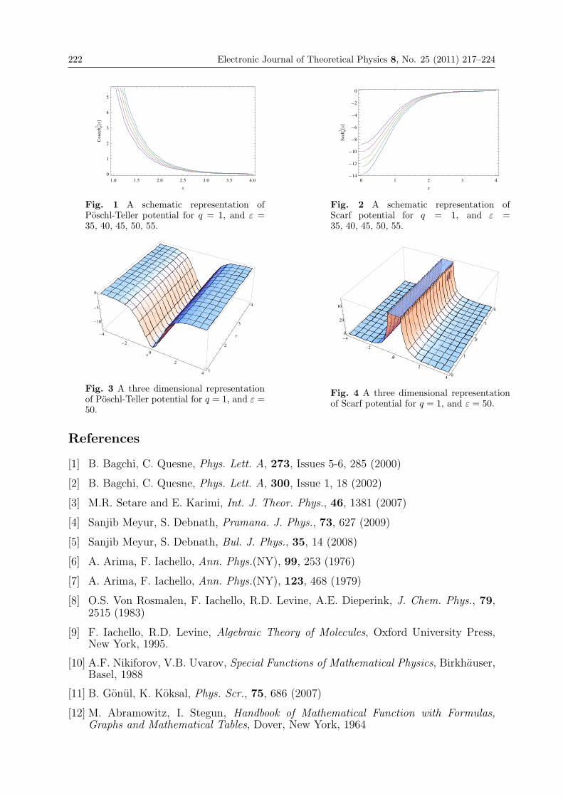
222 Electronic Journal of Theoretical Physics 8, No. 25 (2011) 217–224
1.0 1.5 2.0 2.5 3.0 3.5 4.00
1
2
3
4
5
x
Cos
ech q2 �
x�
Fig. 1 A schematic representation ofPoschl-Teller potential for q = 1, and ε =35, 40, 45, 50, 55.
0 1 2 3 4�14
�12
�10
�8
�6
�4
�2
0
x
Sech
q2 �x�
Fig. 2 A schematic representation ofScarf potential for q = 1, and ε =35, 40, 45, 50, 55.
�4
�2
0
2
4
x
1
2
3
4
y
�10
�5
0
Fig. 3 A three dimensional representationof Poschl-Teller potential for q = 1, and ε =50.
�4
�2
0
2
4
x
0
1
2
3
4
y0
20
40
Fig. 4 A three dimensional representationof Scarf potential for q = 1, and ε = 50.
References
[1] B. Bagchi, C. Quesne, Phys. Lett. A, 273, Issues 5-6, 285 (2000)
[2] B. Bagchi, C. Quesne, Phys. Lett. A, 300, Issue 1, 18 (2002)
[3] M.R. Setare and E. Karimi, Int. J. Theor. Phys., 46, 1381 (2007)
[4] Sanjib Meyur, S. Debnath, Pramana. J. Phys., 73, 627 (2009)
[5] Sanjib Meyur, S. Debnath, Bul. J. Phys., 35, 14 (2008)
[6] A. Arima, F. Iachello, Ann. Phys.(NY), 99, 253 (1976)
[7] A. Arima, F. Iachello, Ann. Phys.(NY), 123, 468 (1979)
[8] O.S. Von Rosmalen, F. Iachello, R.D. Levine, A.E. Dieperink, J. Chem. Phys., 79,2515 (1983)
[9] F. Iachello, R.D. Levine, Algebraic Theory of Molecules, Oxford University Press,New York, 1995.
[10] A.F. Nikiforov, V.B. Uvarov, Special Functions of Mathematical Physics, Birkhauser,Basel, 1988
[11] B. Gonul, K. Koksal, Phys. Scr., 75, 686 (2007)
[12] M. Abramowitz, I. Stegun, Handbook of Mathematical Function with Formulas,Graphs and Mathematical Tables, Dover, New York, 1964

Electronic Journal of Theoretical Physics 8, No. 25 (2011) 217–224 223
[13] I.S. Gradshteyn, I.M. Ryzhik, Tables of Integrals, Series and Products, AP, NewYork, 1980.
[14] W. Magnus, F. Oberhettinger, R.P. Soni, Formulas and Theorems for the SpecialFunction of Mathematical Physics, 3rd ed., Springer, Berlin, 1966
[15] Y.F. Cheng, T.Q. Dai, Phys. Scr., 75, 274 (2007)
[16] C.Y. Chen, S.H. Dong, Phys. Lett. A, 335, 374 (2005)
[17] Sanjib Meyur, S. Debnath, Bul. J. Phys., 36, volume 1 17 (2009)
[18] Sanjib Meyur, S. Debnath, Bul. J. Phys., 35, volume 4, 290 (2008)


EJTP 8, No. 25 (2011) 225–232 Electronic Journal of Theoretical Physics
Bound State Solutions of the Klein Gordon Equationwith the Hulthen Potential
Akpan N. Ikot∗1, Louis E. Akpabio1 and Edet J. Uwah2
1Department Of Physics, University Of Uyo, Nigeria2Department Of Physics, University Of Calabar, Nigeria
Received 6 July 2010, Accepted 10 February 2011, Published 25 May 2011
Abstract: An approximate solution of the Klein–Gordon equation for the Hulthen potential
with equal scalar and vector potential is presented. Using the new improved approximation
scheme to deal with the centrifugal term, we solve approximately the Klein–Gordon equation
via the Nikiforov–Uvarov method for an arbitrary angular momentum quantum number. The
corresponding eigen – energy and eigen functions are also obtained for the s-wave bound state.c© Electronic Journal of Theoretical Physics. All rights reserved.
Keywords: Klein Gordon Equation; Approximation Scheme; Hulthen Potential
PACS (2010): 03.65.Pm; 02.60.Lj; 03.65.Pm; 02.30.Jr
1. Introduction
In recent times the Nikiforov-Uvarov (NU) method has been used successfully in solving
the Schrodinger, Dirac, Klein-Gordon, and Duffin-Kemmer-Petiau wave equations in the
presence of some well known potential [1-5]. In relativistic mechanics, the solution of the
Klein-Gordon and Dirac equation with some physical potential play a significant role in
nuclear physics and other areas [6,7]. These relativistic equations contain two objects,
the vector V(r) and scalar potential S(r).
The Klein-Gordon equation with the vector and scalar potentials can be written as
follows: [−(i∂
∂t− V (r)
)2
−∇2 + (S(r) +M)2]ψ(r, θ, ϕ) = 0 (1)
where M is the rest mass and for the case S(r) = ±V (r) has been studied recently [8,9].However, the analytical solutions of the Klein-Gordon equations are possible only

226 Electronic Journal of Theoretical Physics 8, No. 25 (2011) 225–232
in the s-wave case with the angular momentum � = 0 for some exponential type po-
tential models [10-11]. Conversely, when � �= 0, one can only solve approximately the
Klein-Gordon equations and the Dirac equation for some potential by using a suitable
approximation scheme [6]. Generalized Hulthen potential which is reducible to the stan-
dard Hulthen potential, Woods-Saxon potential, exponential type screened potentials are
studied [6,12]. The bound states relativistic solution of the standard Hulthen potential
has also been presented [13,14].
With the conventional approximation scheme suggested by Greene and Aldrich [15]
to deal with the centrifugal term, many authors have evaluated the bound state solutions
of the Klein-Gordon and Dirac equations for different potentials [6,16].
The method Nikiforov-Uvarov (NU) [17] is based on solving the second order linear
differential equations by reducing to a generalized equation of hypergeometric type. The
NU-method is used to solve the Schrodinger, Klein-Gordon, Dirac and Duffin-Kemmer-
Petiau equations with exponential-like potentials such as Woods-Saxon [18], Hulthen [19]
and Poschl – Teller [20].
Motivated by the success in obtaining approximately the bound state solution of the
Klein-Gordon equation with Poschl-Teller potential [21]. We attempt to solve approx-
imately the arbitrary l−wave Klein-Gordon equation with Hulthen potential using the
NU-method. The centrifugal term in the Klein-Gordon equation is deal with using a new
improved approximation scheme [26].
2. Nikiforov-Uvarov Method
The NU method [17] is based on the solution of a generalized second order linear differ-
ential equation with special orthogonal functions [22]. The Schrodinger equation
ψ′′(x) + [E − V (x)]ψ(x) = 0, (2)
can be solved by this method. This can be done by transforming this equation of hyper-
geometric type with appropriate co-ordinate transformation, s = s(x).
ψ′′(s) +τ(s)
σ(s)ψ′(s) +
σ(s)
σ2(s)ψ(s) = 0 (3)
In order to find the exact solution to equation (3), we set the wave function as
ψ(s) = ϕ(s)χ(s), (4)
and on substituting, equation (4) into equation (3) reduces equation (3) into hypergeo-
metric type,
σ(s)χ′′(s) + τ(s)χ′(s) + λχ(s) = 0 (5)
where the wave function ψ(s) is defined as the logarithmic derivative [23]
ϕ1(s)
ϕ(s)=π(s)
σ(s), (6)

Electronic Journal of Theoretical Physics 8, No. 25 (2011) 225–232 227
where π(s) is at most first-degree polynomials.
Likewise, the hypergeometric type function χ(s) in equation (5) for a fixed n is given
by the Rodrigues relation
χn(s) =Bn
ρ(s)
dn
dsn[σ′′(s)ρ(s)] , (7)
where Bn is the normalization constant and the weight function ρ(s) most satisfy the
condition [17]d
ds(σ(s)ρ(s)) = τ(s)ρ(s), (8)
with
τ(s) = τ(s) + 2π(s) (9)
In order to accomplish the conditions imposed on the weight function ρ(s), it is necessary
that the classical orthogonal polynomials τ(s) be equal to zero to some point of an interval
(a, b) and its derivative at this interval at σ(s) > 0 will be negative, that is
dτ(s)
ds< 0. (10)
Therefore, the function π(s) and the parameter λ required for the NU-method are defined
as follows:
π(s) =σ′ − τ
2±
√(σ′ − τ
2
)2
− σ + kσ, (11)
λ = k + π′(s) (12)
The k-values in equation (11) are possible to evaluate if the expression under the square-
root must be square of polynomials. This is possible, if and only if its discriminant is
zero. With this, a new eigen-value equation becomes
λ = λn = −ndτ
ds− n (n− 1)
2
d2σ
ds2, n = 0, 1, 2, ... (13)
where τ(s) is as defined in equation (9) and on comparing equation (12) and equation
(13), we obtain the energy eigen values.
3. Bound State Solutions of Klein-Gordon Equation
The three-dimensional Klein-Gordon equation with vector V(r) and scalar potential S(r)
can be written as[∇2 + (V (r)− E)2 − (S(r) +M)2
]ψ (θ, r, ϕ) = 0, (14)
where E is the relativistic energy; ∇2 is the Laplace operator and where the velocity of
light and Planck’s constants have been set to unity. Writing the total spherical wave
function as
ψ (r, θ, ϕ) =1
rR(r)Y (θ, ϕ), (15)

228 Electronic Journal of Theoretical Physics 8, No. 25 (2011) 225–232
separated equation (14) into variables and the resulting equations become [24]
d2
dr2R(r) + 2
[MS(r) + EV (r) + S2(r)− V 2(r) +
�(�+ 1)
r2
](16)
R(r) =(E2 −M2
)R(r) (17)
d2Θ(θ)
dθ2+ cot θ
d
dθΘ(θ) +
[λ− m2
sin2 θ− (E +M)
]Θ(θ) (18)
d2Φ(ϕ)
dϕ2+m2Φ(ϕ) = 0, (19)
where Y (θ, ϕ) = Θ(θ)Φ(ϕ) and m2 is the separate content, λ = �(�+ 1).
The solution to equation (17) and (18) are well known, [25].
4. Solution of the Radial Equation via Nu-Method
The Hulthen potential is defined by
V (r) =−V0e−2αr(1− e−2αr)
, (20)
where V0 is the potential depth and α is an arbitrary constant. The radial equation of
the Klein-Gordon equation for the special case V(r) = S(r) is
d2R(r)
dr2+
[V0e
−2αr
(1− e−2αr)(M + E) +
�(�+ 1)
r2
]R(γr) =
(E2 −M2
)R(r) (21)
The centrifugal term in equation (21) can be evaluated using the new improved approx-
imation scheme [26]. However, with the centrifugal term present, equation (21) can not
be solve analytically, that is for� �= 0. In order to obtain the approximate analytical
solutions of equation (21) for� �= 0, we follow the new improved approximation scheme
[26] to deal with the centrifugal term
1
r2≈ 4α2
[c0 +
e−2αr
(1− e−2αr)2
], (22)
where c0 =12is an arbitrary dimensionless constant. In this study, we set c0=0 which
reduces the new improved approximation scheme to conventional approximation scheme
suggested by Green and Aldrich [15].
Substituting equation (22) into equation (21) yields.
d2R(r)
dr2+
[E2 +
V1e−2αr
(1− e−2αr)+4α2�(�+ 1)e−2αr
(1− e−2αr)2
]R(r) = 0 (23)
where V1 = (E +M)V0 and E2 = (E2 −M2).

Electronic Journal of Theoretical Physics 8, No. 25 (2011) 225–232 229
Introducing a new variable s = e−2αr, reduces equation (23) into hypergemetric type,
d2R
ds2+1
s
(1− s)
(1− s)
dR
ds+
1
s2(1− s)2[−ε2s2 +
(2ε2 − β2 + γ2
)s+ β2 − ε2
]R(s) = 0 (24)
where the following dimensionless quantity has been used in obtaining equation (24);
ε2 = − E2
2α2, β2 =
V12α2
, γ2 = 2�(�+ 1). (25)
Now comparing equation (24) with equation (3), we get
σ(s) = s(1− s), τ(s) = (1− s),
σ(s) = −ε2s2 +(2ε2 − β2 + γ2
)s+ β2 − ε2. (26)
Substituting equation (26) into equation (11) yields
π(s) = −s2± 1
2
√(4ε2 − 4k + 1) s2 + 4 (β2 − 2ε2 − γ2 + k) s+ 4 (ε2 − β2), (27)
and we get two possible functions for each root k as
π(s) = −s2± 1
2
⎧⎪⎪⎪⎪⎪⎪⎪⎪⎪⎪⎪⎨⎪⎪⎪⎪⎪⎪⎪⎪⎪⎪⎪⎩
(2√ε2 − β2 − i
√γ2 + 1
4
)s− 2
√ε2 − β2,
for k = β2 + γ2 +√(ε2 − β2)
(−γ2 − 1
4
)(2√ε2 − β2 + i
√γ2 + 1
4
)s− 2
√ε2 − β2,
for k = β2 + γ2 −√(ε2 − β2)
(−γ2 − 1
4
)(28)
From the four possible forms of the polynomials π(s), we select the one for which the
τ ′(s) < 0, thus, using equation (9), we get
τ(s) = 1− 3s
(√ε2 − β2 + i
√γ2 +
1
4
)s−
√ε2 − β2
τ ′(s) = −3−(√
ε2 − β2 + i
√γ2 +
1
4
). (29)
Therefore, the appropriate π(s) value is
π(s) = −s2− 1
2
[(2√ε2 − β2 + i
√γ2 +
1
4
)s− 2
√ε2 − β2
]. (30)
The constant λ = k + π′(s) is obtain as
λ = β2 + γ2 − i
√(ε2 − β2)
(γ2 +
1
4
)+1
2−√ε2 − β2 − i
√γ2 +
1
4, (31)

230 Electronic Journal of Theoretical Physics 8, No. 25 (2011) 225–232
and from the definition of λn, we write
λn = 2n+ 2n√ε2 − β2 + in
√γ2 +
1
4+ n(n− 1). (32)
On comparing equations (31) and (32), we obtain the bound state eigen energy for the
Klein-Gordon equation as
E = − V12α2
− 2α2
⎡⎢⎣(
V1
2α2
)(1 + 2n+ i
√γ2 + 1
4
) +2�(�+ 1)(
1 + 2n+ i√γ2 + 1
4
)
+1
2(1 + 2n+ i
√γ2 + 1
4
) − n+ i (1 + n)√γ2 + 1
4(1 + 2n+ i
√γ2 + 1
4
)⎤⎥⎦
2
. (33)
The corresponding wave function can now be calculated by first calculating the weight
function in equation (8) as
d
ds(σ(s)ρ(s)) = τ(s)ρ(s), (34)
yields
ρ(s) = (1− s)2√
ε2−β2+1(1 + s)i√
γ2+ 14 . (35)
Substituting equation (35) into the Rodrigues relation of equation (7), we obtain the
eigen function χn(s) as
χn(s) = Bn(1 + s)−i
(√γ2+ 1
4
)(1− s)
−(2√
ε2−β2+1)
× dn
dsn
[(1− s2
)n(1− s)
−(2√
ε2−β2+1)(1 + s)−i
√γ2+ 1
4
]= BnP
(μ,υ)n (s), (36)
where Bn is the normalization constant and μ = i√γ2 + 1
4and υ = 2
√ε2 − β2 + 1 and
Pn(s) is the Jacobi polynomials.
The other part of the wave function in equation (6) is obtained by using ϕ′(s)ϕ(s)
= π(s)σ(s)
and solving the differential equation yields,
ϕ(s) = (1− s)2√
ε2−β2+ 12 (1 + s)i
√γ2+ 1
4 (37)
Combining the Jacobi polynomials and equation (37), we obtain the wave function as
ψn(s) = An (1− s)2v (1 + s)μ P (μ,v)n (s), (38)
where An is a new normalization constant.

Electronic Journal of Theoretical Physics 8, No. 25 (2011) 225–232 231
Conclusions
The solution of the radial Klein-Gordon equation for the Hulthen potentials with an
arbitrary angular momentum � �= 0 are obtained. Using the NU method, we obtain
the approximate solution of the Klein-Gordon equation with equal scalar and vector
potentials for s-wave bound state. By using a new improved approximation approach
to deal with the centrifugal term, we obtain approximately the energy eigen value and
the unnormalized radial eigen function in terms of the hypergeometric function for an
arbitrary l-states.
Acknowledgement
This research was supported by the grant NANDY-LEABIO 2474.
References
[1] H. Egrifes, D. Demirhan and F. Buyukkihe, Phys. Scri. 59, 90, (1999).
[2] N. Cotfas, J. Phys. A: Math. Gen. 35, 9355 (2002).
[3] O. Yesiltas, M. Simsek, R. Sever and C. Tezcan, Phys. Scr. 67, 472 (2003).
[4] A. Berkdemir, C. Berkdemir and R. Sever. Phys. Rev. C, 72, 27001 (2004).
[5] C. Berkdemir, Nucl. Phys. A. 770. 32 (2006).
[6] Y. Xu, S. He and C. S. Jia, Phys. Scr. 81, 045001 (2010).
[7] M. Simsek and H. Egrifes, J. Phys. Lon. Math. Gen. 27, 4379 (2004).
[8] A. D. Alhaidari, H. Bahlouli and A. M-Hasan, Phys. Lett. A., 349, 87, (2006).
[9] F. Yasuk, A. Durmus and I. Boztosun, arxiv: quant-ph/0606224, (2006).
[10] Y. F. Diao, L. Z. Yi and C. S. Jia, Phys. Lett. A. 332, 157, (2004).
[11] X. Zou, L. Z. Yi and C. S. Jia, Phys. Lett. A. 346, 54. (2005).
[12] H. Egrifes and R. Sever, Int. J. Theor. Phys. 46, 935 (2007).
[13] F. Dominguez - Adame, Phys. Lett. A. 136, 175 (1989).
[14] L. Chetouani, L. Guechi, A. Lecheheb, T. F. Hamman and A. Messouber, Physica,A. 234, 529, (1996).
[15] R. L. Greene and C. Aldrich, Phys. Rev. A. 14, 2363, (1976).
[16] N. Sadd, Phys. Scri. 76 623 (2007).
[17] A. F. Nikiforov and V. B. Uvarov, Special Functions of Mathematical Physics (Basel,Birkhauser,1988).
[18] A. Berkdemir, C. Berkdemir and R. Sever, Mod. Phys. Lett. A. 21, 2087 (2006).
[19] F. Yasuk, C. Berkdemir, A. Berkdemir and C. Onem, Phys. Scr. 71, 340 (2005).
[20] O. Yesiltas, Phys. Scr. 75, 4146 (2007).

232 Electronic Journal of Theoretical Physics 8, No. 25 (2011) 225–232
[21] T. Chen, J. Y. Liu and C. S. Jia, Phys. Scr. 79, 055002 (2009).
[22] A. F. Nikiforov, S. K. Suslov and V. B. Uvarov, Classical orthogonal polynomials ofa discrete variables (Springer, Berlin, 1991).
[23] N. Cotfas, CEJP, 2, L1195 (2004).
[24] S. Flugge, Practical Quantum Mechanics, (Springer, Berlin, 1974).
[25] J. Sadeghi and B. Pourhassan, EJTP 5, 193 (2008).
[26] C. S. Jia, T. Chen and L. G. Cui, Phys. Lett. A. 373, 1621 (2009).

EJTP 8, No. 25 (2011) 233–244 Electronic Journal of Theoretical Physics
Chaotic dynamics of the Fractional OrderNonlinear Bloch System
Nasr-eddine Hamri∗1 and Tarek Houmor†2
1Institute of Sciences & Technologie, University Center of Mila, Algeria2Department of Mathematics, University of Constantine, Algeria
Received 6 July 2010, Accepted 10 February 2011, Published 25 May 2011
Abstract: The dynamic behaviors in the fractional-order nonlinear Bloch equations were
numerically studied. Basic properties of the system have been analyzed by means of Lyapunov
exponents and bifurcation diagrams. The derivative order range used was relatively broad.
Regular motions (including period-3 motion) and chaotic motions were examined. The chaotic
motion identified was validated by the positive Lyapunov exponent.c© Electronic Journal of Theoretical Physics. All rights reserved.
Keywords: Dynamical Systems; Fractional Calculus; Bifurcation
PACS (2010): 05.45.Pq; 05.45.Xt; 05.45.-a; 05.45.-a; 02.30.Oz
1. Introduction
The dynamics of fractional-order systems have attracted increasing attentions in recent
years. It has been shown that the fractional-order generalizations of many well-known
systems can also behave chaotically: [12] and [7] for the fractional Chua system, [3] and
[17] for the fractional Duffing one, [8] and [9] for the fractional Chen one and so on.
A review of the literature indicates that phase portrait, bifurcation diagram, Poincare
maps and Lyapunov exponent always be the efficient ways to research the integer and
fractional-order systems. Many investigations about fractional-order system have been
done. Many researches to nonlinear fractional-order equations are based on the frequency-
domain method whereas there are some disadvantages of using this method were found
in [19]. On the other hand, the dynamic properties in fractional systems are still needing
pay more attentions, some basic properties such as fixed point, limit cycles and chaos
have been investigated. Bifurcation, Poincare map and Lyapunov exponent are all good
∗ [email protected]† tarek [email protected]

234 Electronic Journal of Theoretical Physics 8, No. 25 (2011) 233–244
tools.
In this paper, the dynamics of the fractional-order nonlinear Bloch system is studied.
Nonlinear Bloch system is a system of three nonlinear ordinary differential equations,
which define a continuous-time dynamical system that exhibits chaotic dynamics associ-
ated with the fractal properties of the attractor.
In the paper, we will focus on the dynamical behavior of fractional-order nonlinear
Bloch system. Experience of dynamical behavior will be considered. Bifurcation of
the parameter-dependent system which provides a summary of essential dynamics is in-
vestigated. Period-3 windows, coexisting limit cycles and chaotic zones are found. The
occurrence and the nature of chaotic attractors are verified by evaluating the largest Lya-
punov exponents. This paper is organized as follows. Fractional derivative definitions, a
method for solving fractional-order differential equation and some stability results are in-
troduced in Section 2. In Section 3, fractional-order nonlinear Bloch system is presented
based on the integer-order system. Bifurcation and the largest Lyapunov exponents of the
fractional-order nonlinear Bloch system are studied in Section 4. Finally, some concluding
remarks are given in Section 5.
2. Fractional Calculus Fundamentals
2.1 Definitions of Fractional Derivatives
The idea of fractional calculus has been known since the development of the regular
calculus, with the first reference probably being associated with Leibniz and L’Hospital
in 1695 where half-order derivative was mentioned. Fractional calculus is a generalization
of integration and differentiation to non-integer order fundamental operator aDrt , where
a and t are the limits of the operation. The continuous integro-differential operator is
defined as
aDrt =
⎧⎪⎪⎪⎪⎨⎪⎪⎪⎪⎩dr
dt: r > 0
1 : r = 0∫ t
a(dτ)−r : r < 0
(1)
The three definitions used for the general fractional differintegral are the Grunwald-
Letnikov (GL) definition, the Riemann-Liouville (RL), and the Caputo definition [11, 13].
These definitions are equivalent for a wide class of functions [13]. The GL is given as
aDrt f(t) = lim
h→0h−r
[ t−ah
]∑j=0
(−1)j
⎛⎜⎝ r
j
⎞⎟⎠ f(t− jh), (2)
where [.] means the integer part. The RL definition is given as
aDrt f(t) =
1
Γ(n− r)
dn
dtn
∫ t
a
f(τ)
(t− τ)r−n+1dτ, (3)

Electronic Journal of Theoretical Physics 8, No. 25 (2011) 233–244 235
for (n − 1 < r < n) and where Γ(.) is the Gamma function.The Caputo’s definition can
be written as
aDrt f(t) =
1
Γ(n− r)
∫ t
a
f (n)(τ)
(t− τ)r−n+1dτ, (4)
for(n − 1 < r < n). The initial conditions for the fractional order differential equations
with the Caputo’s derivatives are the same form as for the integer-order differential equa-
tions. These integer-order derivatives have a physical meaning and can be measured. On
the other hand, when the Riemann-Liouville derivative (3) is considered, it is necessary
to specify the values at t0 = 0 in terms of fractional integrals and their derivatives. These
data do not have a physical meaning and, consequently, are not measurable. It can be
concluded that the Caputo derivative (4) is a better choice for our study, since the initial
values required by the Caputo definition coincide with identifiable physical states in our
system.
2.2 Numerical Methods for Calculation of The Fractional Order Deriva-
tives
Since the analysis of fractional-order systems is not sufficient yet, a suitable numerical
method needs to be selected. Among the literature of fractional-order field, two approx-
imation methods have been proposed in order to obtain response of a fractional order
system, one of which is the Adams-Bashforth-Moulton predictor-corrector scheme [5, 6],
while the other one is the frequency domain approximation [4]. Due to the specificity of
the error estimation bound, simulation results obtained by the former method are more
reliable than those of the latter [20]. As a result, the former method is used throughout
this paper because of its efficiency and reliability. The method is based on the fact that
fractional differential equation
Dα∗ y(t) = f(t, y(t)), 0 ≤ t ≤ T,
y(k)(0) = y(k)0 , k = 0, 1, ...,m− 1
(5)
is equivalent to the Volterra integral equation
y(t) =
[α]−1∑k=0
y(k)(0)tkn+1
k!+
1
Γ(α)
∫ t
0
(t− s)α−1f(s, y(s))ds (6)
Set h = (T/N), tn = nh, n = 0, 1, ...N ∈ Z+.
Then (6) can be discretized as follows:
yh(tn+1) =
[α]−1∑k=0
y(k)(0)tkn+1
k!+
hα
Γ(α + 2)f(tn+1, y
ph(tn+1) +
+hα
Γ(α + 2)
n∑j=0
aj,n+1f(tj, yh(tj)) (7)
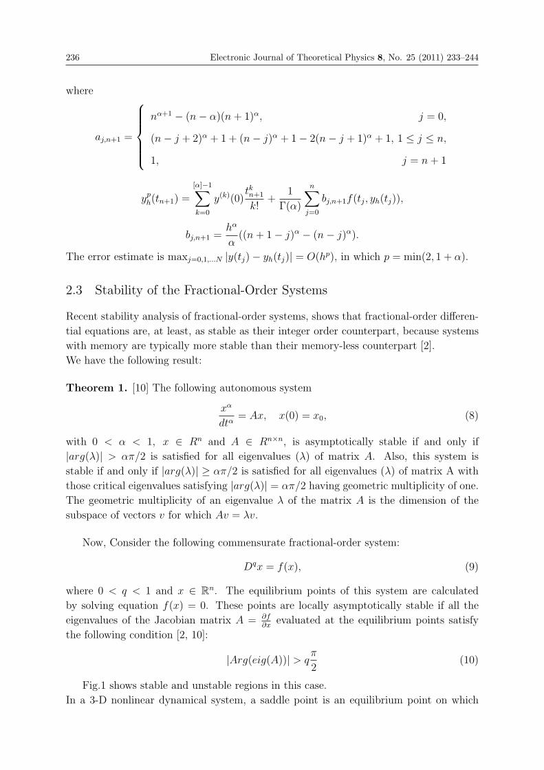
236 Electronic Journal of Theoretical Physics 8, No. 25 (2011) 233–244
where
aj,n+1 =
⎧⎪⎪⎪⎪⎨⎪⎪⎪⎪⎩nα+1 − (n− α)(n+ 1)α, j = 0,
(n− j + 2)α + 1 + (n− j)α + 1− 2(n− j + 1)α + 1, 1 ≤ j ≤ n,
1, j = n+ 1
yph(tn+1) =
[α]−1∑k=0
y(k)(0)tkn+1
k!+
1
Γ(α)
n∑j=0
bj,n+1f(tj, yh(tj)),
bj,n+1 =hα
α((n+ 1− j)α − (n− j)α).
The error estimate is maxj=0,1,...N |y(tj)− yh(tj)| = O(hp), in which p = min(2, 1 + α).
2.3 Stability of the Fractional-Order Systems
Recent stability analysis of fractional-order systems, shows that fractional-order differen-
tial equations are, at least, as stable as their integer order counterpart, because systems
with memory are typically more stable than their memory-less counterpart [2].
We have the following result:
Theorem 1. [10] The following autonomous system
xα
dtα= Ax, x(0) = x0, (8)
with 0 < α < 1, x ∈ Rn and A ∈ Rn×n, is asymptotically stable if and only if
|arg(λ)| > απ/2 is satisfied for all eigenvalues (λ) of matrix A. Also, this system is
stable if and only if |arg(λ)| ≥ απ/2 is satisfied for all eigenvalues (λ) of matrix A with
those critical eigenvalues satisfying |arg(λ)| = απ/2 having geometric multiplicity of one.
The geometric multiplicity of an eigenvalue λ of the matrix A is the dimension of the
subspace of vectors v for which Av = λv.
Now, Consider the following commensurate fractional-order system:
Dqx = f(x), (9)
where 0 < q < 1 and x ∈ Rn. The equilibrium points of this system are calculated
by solving equation f(x) = 0. These points are locally asymptotically stable if all the
eigenvalues of the Jacobian matrix A = ∂f∂x
evaluated at the equilibrium points satisfy
the following condition [2, 10]:
|Arg(eig(A))| > qπ
2(10)
Fig.1 shows stable and unstable regions in this case.
In a 3-D nonlinear dynamical system, a saddle point is an equilibrium point on which

Electronic Journal of Theoretical Physics 8, No. 25 (2011) 233–244 237
the equivalent linearized model has at least one eigenvalue in the stable region and one
eigenvalue in the unstable region. In the same system, a saddle point is called saddle
point of index 1 if one of the eigenvalues is unstable and other eigenvalues are stable.
Also, a saddle point of index 2 is a saddle point with one stable eigenvalue and two
unstable eigenvalues. In chaotic systems, it is proved that scrolls are generated only
around the saddle points of index 2. Moreover, saddle points of index 1 are responsible
only for connecting scrolls [18]. Assume that 3-D chaotic system x = f(x) displays one
scroll attractor. Hence, this system has a saddle point of index 2 encircled by a one-scroll
attractor. Suppose λ = α ± jβ are unstable eigenvalues for this saddle point of index 2.
A necessary condition for fractional system Dqx = f(x) to remain chaotic is keeping the
eigenvalue λ in the unstable region. This means
tan(qπ
2
)>|β|α⇒ q >
2
πtan−1
(|β|α
)(11)
jω
σq π /2q π /2
− q π /2
stable
stable
stable
stable
unstable
unstable
Fig. 1 Stability region of linear fractional-order system with order q.
3. Integer-Order Nonlinear Bloch System
The dynamics of an ensemble of spins usually described by the nonlinear Bloch equation
is very important for the understanding of the underlying physical process of nuclear
magnetic resonance. The basic process can be viewed as the combination of a precession
about a magnetic field and of a relaxation process, which gives rise to the damping of
the transverse component of the magnetization with a different time constant. The basic
model is derived from a magnetization M precessing in the magnetic induction field
B0 in the presence of a constant radiofrequency field B1 with intensity B1 = ω1
γand
frequency ωrf . The following modified nonlinear Bloch equation govern the evolution of

238 Electronic Journal of Theoretical Physics 8, No. 25 (2011) 233–244
the magnetization, ⎧⎪⎪⎪⎪⎪⎨⎪⎪⎪⎪⎪⎩x = δy + γz(xsin(c)− ycos(c))− x
Γ2
y = −δx− z + γz(xcos(c) + ysin(c))− y
Γ2
z = y − γsin(c)(x2 + y2)− z − 1
Γ1
(12)
where the variables are properly scaled [1].
It is easy to visualize that fixed the point (x0, y0, z0) of the above system is given as
x0 = f(z0, γ, c, δ,Γ2), y0 = f(z0, γ, c, δ,Γ2) where z0 is given by
γ2z30 − γ
[2sin(c)
Γ2
+ 2δcos(c) + γ
]z20 +
{1
Γ22
+ δ2 +2γsin(c)
Γ2
+ 2γδcos(c) +Γ1
Γ2
}z0
−(1
Γ22
+ δ2)= 0,
a cubic equation. In particular for real root one can always get the restriction on the
parameters. The jacobian matrix of system (12), evaluated at the equilibrium (x0, y0, z0)
J =
⎛⎜⎜⎜⎜⎜⎝γsin(c)z0 −
1
Γ2
δ − γcos(c)z0 γ (sin(c)x0 − cos(c)y0)
−δ + γcos(c)z0 γsin(c)z0 −1
Γ2
−1 + γ (cos(c)x0 + sin(c)y0)
−2γsin(c)x0 1− 2γsin(c)y0 − 1
Γ1
⎞⎟⎟⎟⎟⎟⎠Previous works shows that the system (12) possess chaotic attractors for two different
sets of parameter values, the first set of parameters is:
γ = 10, δ = 1.26, c = 0.7764, Γ1 = 0.5, Γ2 = 0.25
and the second set:
γ = 35, δ = −1.26, c = 0.173, Γ1 = 5, Γ2 = 2.5
The form of attractors is given in Fig.2.
0.20.4
0.60.8
1
−0.5
0
0.5
1−0.6
−0.4
−0.2
0
0.2
0.4
z(t)x(t)
y(t)
−0.2−0.1
00.1
0.20.3
−0.4
−0.2
0
0.2
−0.4
−0.2
0
0.2
0.4
z(t)
x(t)
y(t)
Fig. 2 Chaotic attractors of system (12) for the parameters: (a) γ = 10, δ = 1.26, c =0.7764, Γ1 = 0.5, Γ2 = 0.25 . (b) γ = 35, δ = −1.26, c = 0.173, Γ1 = 5, Γ2 = 2.5 .
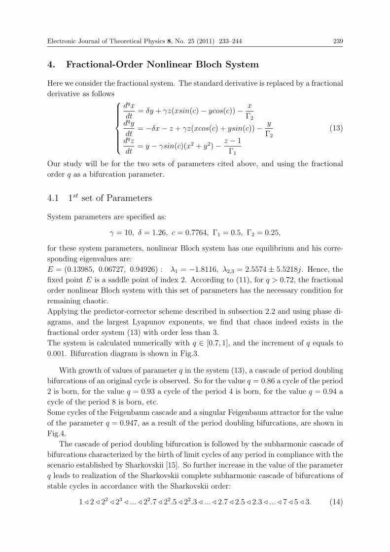
Electronic Journal of Theoretical Physics 8, No. 25 (2011) 233–244 239
4. Fractional-Order Nonlinear Bloch System
Here we consider the fractional system. The standard derivative is replaced by a fractional
derivative as follows⎧⎪⎪⎪⎪⎪⎨⎪⎪⎪⎪⎪⎩
dqx
dt= δy + γz(xsin(c)− ycos(c))− x
Γ2dqy
dt= −δx− z + γz(xcos(c) + ysin(c))− y
Γ2dqz
dt= y − γsin(c)(x2 + y2)− z − 1
Γ1
(13)
Our study will be for the two sets of parameters cited above, and using the fractional
order q as a bifurcation parameter.
4.1 1st set of Parameters
System parameters are specified as:
γ = 10, δ = 1.26, c = 0.7764, Γ1 = 0.5, Γ2 = 0.25,
for these system parameters, nonlinear Bloch system has one equilibrium and his corre-
sponding eigenvalues are:
E = (0.13985, 0.06727, 0.94926) : λ1 = −1.8116, λ2,3 = 2.5574 ± 5.5218j. Hence, the
fixed point E is a saddle point of index 2. According to (11), for q > 0.72, the fractional
order nonlinear Bloch system with this set of parameters has the necessary condition for
remaining chaotic.
Applying the predictor-corrector scheme described in subsection 2.2 and using phase di-
agrams, and the largest Lyapunov exponents, we find that chaos indeed exists in the
fractional order system (13) with order less than 3.
The system is calculated numerically with q ∈ [0.7, 1], and the increment of q equals to
0.001. Bifurcation diagram is shown in Fig.3.
With growth of values of parameter q in the system (13), a cascade of period doubling
bifurcations of an original cycle is observed. So for the value q = 0.86 a cycle of the period
2 is born, for the value q = 0.93 a cycle of the period 4 is born, for the value q = 0.94 a
cycle of the period 8 is born, etc.
Some cycles of the Feigenbaum cascade and a singular Feigenbaum attractor for the value
of the parameter q = 0.947, as a result of the period doubling bifurcations, are shown in
Fig.4.
The cascade of period doubling bifurcation is followed by the subharmonic cascade of
bifurcations characterized by the birth of limit cycles of any period in compliance with the
scenario established by Sharkovskii [15]. So further increase in the value of the parameter
q leads to realization of the Sharkovskii complete subharmonic cascade of bifurcations of
stable cycles in accordance with the Sharkovskii order:
1 � 2 � 22 � 23 � ... � 22.7 � 22.5 � 22.3 � ... � 2.7 � 2.5 � 2.3 � ... � 7 � 5 � 3. (14)

240 Electronic Journal of Theoretical Physics 8, No. 25 (2011) 233–244
0.7 0.75 0.8 0.85 0.9 0.95 1−0.25
−0.2
−0.15
−0.1
−0.05
0
0.05
0.1
0.15
q
x
Fig. 3 Bifurcation diagram with parameter q increasing form 0.7 to 1.
0.70.8
0.91
−0.20
0.20.4
0.6−0.2
−0.1
0
0.1
0.2
0.3
z(t)x(t)
y(t)
q=0.85
0.50.6
0.70.8
0.9
−0.20
0.20.4
0.6−0.4
−0.2
0
0.2
0.4
z(t)x(t)
y(t)
q=0.86
0.40.5
0.60.7
0.80.9
−0.20
0.20.4
0.6−0.4
−0.2
0
0.2
0.4
z(t)x(t)
y(t)
q=0.93
0.20.4
0.60.8
1
−0.20
0.20.4
0.6−0.4
−0.2
0
0.2
0.4
z(t)x(t)
y(t)
q=0.94
0.20.4
0.60.8
1
−0.20
0.20.4
0.6−0.4
−0.2
0
0.2
0.4
z(t)x(t)
y(t)
q=0.947
Fig. 4 Projections of original cycle, period two cycle, period four cycle, period eight cycle andFeigenbaum attractor in the fractional order nonlinear Bloch system.
The ordering n � k in (14) means that the existence of a cycle of period k implies the
existence of all cycles of period n. So, if the system (13) has a stable limit cycle of period
three then it has also all unstable cycles of all periods in accordance with the Sharkovskii
order (14).
The Sharkovskii complete subharmonic cascade of bifurcations of stable cycles is proved
by existence of a limit cycle of period 6 for the parameter value q = 0.948, a limit cycle
of period 5 for q = 0.955 and a limit cycle of period 3 lying in the interval [0.965, 0.979]
which with further increase of the parameter q goes through a cascade of period doubling
bifurcations. Thus, for q = 0.98 we observe a doubled cycle of period 3. The subharmonic
cascade also terminates with the formation of an irregular attractor.
Some cycles of this cascade and a subharmonic singular attractor are shown in Fig.5.
To demonstrate the chaotic dynamics, the largest Lyapunov exponent should be the
first thing to be considered, because any system containing at least one positive Lyapunov
exponent is defined to be chaotic [16]. Measuring the largest Lyapunov exponent (LLE) is
always an important problem whatever in a fractional order system or in an integral-order

Electronic Journal of Theoretical Physics 8, No. 25 (2011) 233–244 241
0.20.4
0.60.8
1
−0.20
0.20.4
0.6−0.4
−0.2
0
0.2
0.4
z(t)x(t)
y(t)
q=0.948
0.20.4
0.60.8
1
−0.20
0.20.4
0.6−0.4
−0.2
0
0.2
0.4
z(t)x(t)
y(t)
q=0.955
0.20.4
0.60.8
1
−0.20
0.20.4
0.6−0.6
−0.4
−0.2
0
0.2
0.4
z(t)x(t)
y(t)
q=0.97
0.20.4
0.60.8
1
−0.20
0.20.4
0.6−0.6
−0.4
−0.2
0
0.2
0.4
z(t)x(t)
y(t)
q=0.98
0.20.4
0.60.8
1
−0.20
0.20.4
0.6−0.6
−0.4
−0.2
0
0.2
0.4
z(t)x(t)
y(t)
q=0.99
Fig. 5 Projections of period six cycle, period five cycle, period three cycle, doubled period threecycle and more complex subharmonic singular attractor in the fractional order nonlinear Blochsystem.
system. Wolf and Jacobian algorithms are the most popular algorithm in calculating the
largest Lyapunov exponent of integer-order system. However, Jacobian algorithm is not
applicable for calculating LLE of a fractional order system, since the Jacobian matrix
of fractional order system is hard to be obtained. As to Wolf algorithm [21] which is
relatively difficult to implement. Therefore, in this paper, the small data sets algorithm
developed by Michael T. Rosenstein etc [14] is chosen to calculating LLE of the Fractional
order nonlinear Bloch system, the diagram is plotted in Fig.6.
0.7 0.75 0.8 0.85 0.9 0.95 1−0.02
−0.015
−0.01
−0.005
0
0.005
0.01
0.015
0.02
0.025
0.03
q
Max
imal
Lya
puno
v E
xpon
ents
Fig. 6 Maximal Lyapunov Exponents versus q form 0.7 to 1 step with 0.01.
4.2 2nd set of Parameters
System parameters are specified as:
γ = 35.0, δ = −1.26, c = 0.173, Γ1 = 5.0, Γ2 = 2.5,
for these system parameters, nonlinear Bloch system has one equilibrium and his corre-
sponding eigenvalues are:

242 Electronic Journal of Theoretical Physics 8, No. 25 (2011) 233–244
E = (0.02730, 0.00429, 0.99847) : λ1 = −0.19971, λ2,3 = 5.6155± 35.685j. Hence, the
fixed point E is a saddle point of index 2. The necessary condition to remain chaotic for
the fractional order nonlinear Bloch system with this set of parameters is q > 0.90.
At q ≈ 0.90 a Hopf bifurcation gives birth to an orbitally stable limit cycle. For cer-
tain parameter values, this limit cycle co-exists with another limit cycle with different
period, each with its basin of attraction. Fig.7 shows the bifurcation diagram against the
parameter q and the coexisting limit cycles for different initial condition
0.88 0.9 0.92 0.94 0.96 0.98 1−0.4
−0.35
−0.3
−0.25
−0.2
−0.15
−0.1
−0.05
0
0.05
q
x
−0.10
0.10.2
0.3 −0.4−0.2
00.2
0.4
−0.4
−0.2
0
0.2
0.4
x(t)z(t)
y(t)
q=0.975
Fig. 7 (a) bifurcation diagram vs q, (b)coexisting limit cycles. Initial conditions: (0.1, 0.1, 0.1)for the thick line and (0.01, 0.01, 0.01) for the thin line.
Fixing the initial conditions at (0.1, 0.1, 0.1) and increasing the parameter q, the initial
period one limit cycle will disappear suddenly and is replaced by a period four limit cycle
at q = 0.99, the two limit cycles goes through a cascade of period doubling bifurcations
which terminates with the formation of irregular attractors as shown in Fig.8.
−0.20
0.20.4
0.6
−0.2−0.1
00.1
0.2−0.2
−0.1
0
0.1
0.2
z(t)x(t)
y(t)
q=0.98
−0.10
0.10.2
0.3
−0.4−0.2
00.2
0.4−0.4
−0.2
0
0.2
0.4
z(t)x(t)
y(t)
q=0.99
−0.10
0.10.2
0.3
−0.4
−0.2
0
0.2
0.4−0.4
−0.2
0
0.2
0.4
y(t)
q=0.9915
−0.2−0.1
00.1
0.20.3
−0.4−0.2
00.2
0.4−0.4
−0.2
0
0.2
0.4
z(t)x(t)
y(t)
q=0.9923
−0.050
0.050.1
0.150.2
−0.2−0.1
00.1
0.2
−0.3
−0.2
−0.1
0
0.1
0.2
0.3
z(t)x(t)
y(t)
q=0.994
−0.2−0.1
00.1
0.20.3
−0.4−0.2
00.2
0.4−0.4
−0.2
0
0.2
0.4
z(t)x(t)
y(t)
q=0.995
Fig. 8 Projections of the period doubling bifurcations and irregular attractors.
The largest Lyapunov exponents are calculated numerically with q ∈ [0.85, 1] for an
increment of 0.01 which are plotted in Fig.9.
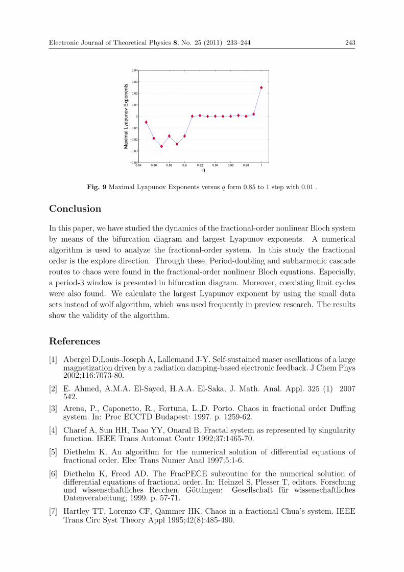
Electronic Journal of Theoretical Physics 8, No. 25 (2011) 233–244 243
0.84 0.86 0.88 0.9 0.92 0.94 0.96 0.98 1−0.04
−0.03
−0.02
−0.01
0
0.01
0.02
0.03
0.04
q
Max
imal
Lya
puno
v E
xpon
ents
Fig. 9 Maximal Lyapunov Exponents versus q form 0.85 to 1 step with 0.01 .
Conclusion
In this paper, we have studied the dynamics of the fractional-order nonlinear Bloch system
by means of the bifurcation diagram and largest Lyapunov exponents. A numerical
algorithm is used to analyze the fractional-order system. In this study the fractional
order is the explore direction. Through these, Period-doubling and subharmonic cascade
routes to chaos were found in the fractional-order nonlinear Bloch equations. Especially,
a period-3 window is presented in bifurcation diagram. Moreover, coexisting limit cycles
were also found. We calculate the largest Lyapunov exponent by using the small data
sets instead of wolf algorithm, which was used frequently in preview research. The results
show the validity of the algorithm.
References
[1] Abergel D,Louis-Joseph A, Lallemand J-Y. Self-sustained maser oscillations of a largemagnetization driven by a radiation damping-based electronic feedback. J Chem Phys2002;116:7073-80.
[2] E. Ahmed, A.M.A. El-Sayed, H.A.A. El-Saka, J. Math. Anal. Appl. 325 (1) 2007542.
[3] Arena, P., Caponetto, R., Fortuna, L.,D. Porto. Chaos in fractional order Duffingsystem. In: Proc ECCTD Budapest: 1997. p. 1259-62.
[4] Charef A, Sun HH, Tsao YY, Onaral B. Fractal system as represented by singularityfunction. IEEE Trans Automat Contr 1992;37:1465-70.
[5] Diethelm K. An algorithm for the numerical solution of differential equations offractional order. Elec Trans Numer Anal 1997;5:1-6.
[6] Diethelm K, Freed AD. The FracPECE subroutine for the numerical solution ofdifferential equations of fractional order. In: Heinzel S, Plesser T, editors. Forschungund wissenschaftliches Recchen. Gottingen: Gesellschaft fur wissenschaftlichesDatenverabeitung; 1999. p. 57-71.
[7] Hartley TT, Lorenzo CF, Qammer HK. Chaos in a fractional Chua’s system. IEEETrans Circ Syst Theory Appl 1995;42(8):485-490.
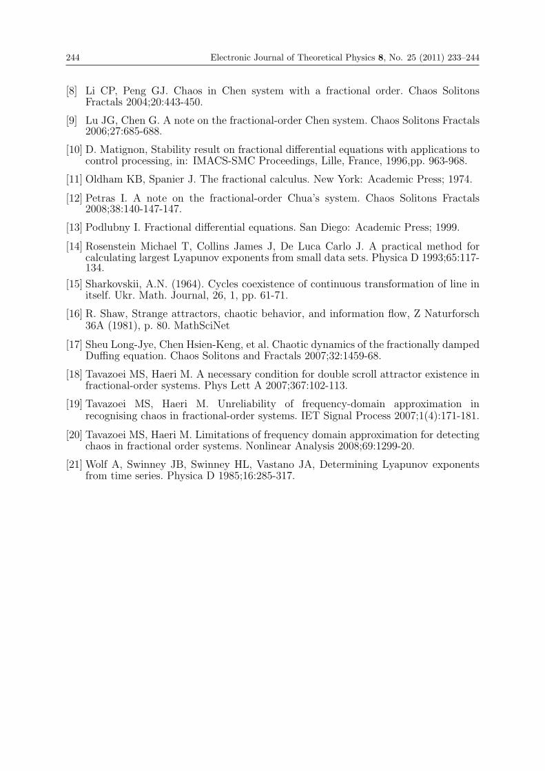
244 Electronic Journal of Theoretical Physics 8, No. 25 (2011) 233–244
[8] Li CP, Peng GJ. Chaos in Chen system with a fractional order. Chaos SolitonsFractals 2004;20:443-450.
[9] Lu JG, Chen G. A note on the fractional-order Chen system. Chaos Solitons Fractals2006;27:685-688.
[10] D. Matignon, Stability result on fractional differential equations with applications tocontrol processing, in: IMACS-SMC Proceedings, Lille, France, 1996,pp. 963-968.
[11] Oldham KB, Spanier J. The fractional calculus. New York: Academic Press; 1974.
[12] Petras I. A note on the fractional-order Chua’s system. Chaos Solitons Fractals2008;38:140-147-147.
[13] Podlubny I. Fractional differential equations. San Diego: Academic Press; 1999.
[14] Rosenstein Michael T, Collins James J, De Luca Carlo J. A practical method forcalculating largest Lyapunov exponents from small data sets. Physica D 1993;65:117-134.
[15] Sharkovskii, A.N. (1964). Cycles coexistence of continuous transformation of line initself. Ukr. Math. Journal, 26, 1, pp. 61-71.
[16] R. Shaw, Strange attractors, chaotic behavior, and information flow, Z Naturforsch36A (1981), p. 80. MathSciNet
[17] Sheu Long-Jye, Chen Hsien-Keng, et al. Chaotic dynamics of the fractionally dampedDuffing equation. Chaos Solitons and Fractals 2007;32:1459-68.
[18] Tavazoei MS, Haeri M. A necessary condition for double scroll attractor existence infractional-order systems. Phys Lett A 2007;367:102-113.
[19] Tavazoei MS, Haeri M. Unreliability of frequency-domain approximation inrecognising chaos in fractional-order systems. IET Signal Process 2007;1(4):171-181.
[20] Tavazoei MS, Haeri M. Limitations of frequency domain approximation for detectingchaos in fractional order systems. Nonlinear Analysis 2008;69:1299-20.
[21] Wolf A, Swinney JB, Swinney HL, Vastano JA, Determining Lyapunov exponentsfrom time series. Physica D 1985;16:285-317.

EJTP 8, No. 25 (2011) 245–252 Electronic Journal of Theoretical Physics
A Criterion for the Stability Analysis of PhaseSynchronization in Coupled Chaotic System
Hadi Taghvafard∗1 and G. H. Erjaee†1,2
1Mathematics Department, Shiraz University, Shiraz, Iran2Mathematics Department, Qatar University, Doha, Qatar
Received 6 July 2010, Accepted 10 February 2011, Published 25 May 2011
Abstract: We report phase synchronization for the coupled diffusionless Lorenz system and for
a new coupled chaotic system in four dimensional space. Stability is also examined by applying
a measure to the linearlized evaluation difference matrix between coupled chaotic systems.c© Electronic Journal of Theoretical Physics. All rights reserved.
Keywords: Chaos; Chaotic Systems; Synchronization; Nonlinear Dynamics
PACS (2010): 05.45.Pq; 05.45.Xt; 05.45.-a
1. Introduction
Recently, synchronization phenomena in coupled chaotic systems have received much at-
tention [1 -17]. Pecora and Carroll have shown [1-4] that in coupled chaotic systems a
complete synchronization occurs if the difference between the various states of synchro-
nized systems converges to zero. They have also shown that synchronization stability
depends upon the signs of the conditional Lyapunov exponents: i.e., if all of the Lya-
punov exponents of the response system under the action of the driver are negative, then
there is a complete and stable synchronization between the drive and response systems.
Synchronization stability can also be verified using the Jacobian matrix in the linearized
state difference between the drive and response chaotic systems [6]. Accordingly, despite
the stability analysis in dynamical systems, if this Jacobian matrix is of full rank and all
of its real parts of eigenvalues are negative, then the system will converge to zero, yield-
ing complete synchronization. Phase synchronization is another type of synchronization
phenomenon which occurs when the Jacobian matrix has some zero eigenvalues. In this
∗ Email:[email protected]† Corresponding author, Email:[email protected]

246 Electronic Journal of Theoretical Physics 8, No. 25 (2011) 245–252
case, the difference between various states of synchronized systems may not necessary
converging to the zero, but will stay less than or equal to a constant.
The main goal of this paper is to discuss the stability analysis of phase synchronization
in coupled chaotic systems which coupled by the nonlinear feedback function method
[18]. Thus, a brief discussion of the nonlinear coupling feedback function method is
presented in section 2, followed by the presentation of a criterion for the stability of
phase synchronization in section 3. In section 4, we presented two numerical examples
to corroborate our analytical assertion.
2. Phase Synchronization
We shall apply the nonlinear coupling feedback function method introduced by Ali and
Fang [18] to coupled chaotic systems. Consider the differential equation x(t) = F(x(t)),
where F(x(t)) is a vector-valued function and decomposed into linear, A(x(t)), and non-
linear, N(x(t)), components, i.e.
F(x(t)) = A(x(t))−N(x(t)). (1)
Now consider two chaotic dynamical systems whose associated vector functions are
decomposed as in (1) and coupled by using the non-linear parts of their vector functions
as follows.
x1(t) = A(x1(t))−N(x1(t)) + r[N(x1(t))−N(x2(t))], (2)
x2(t) = A(x2(t))−N(x2(t)) + r[N(x2(t))−N(x1(t))]. (3)
Here, systems (2) and (3) serve as drive and response systems, respectively, and the
parameter r measures the strength of their coupling. The stability of the synchronization
can be studied by using the evolutional equation of the difference between systems (2)
and (3). This equation is determined by the linear approximation
x(t) =
[A+ (2r − 1)
∂N
∂x
]e(t), (4)
where e(t) = x1(t) − x2(t). It is well-known from linear stability theory in dynamical
systems that if r = 1/2, then the stability type of the zero equilibrium in Equation (4)
reflects the stability type of the synchronization between the two chaotic systems (2), (3)
and depends upon the signs of the real parts of the eigenvalues of A [19]. However, in the
case of phase synchronization, we are not able to use this criterion for stability because
some of these eigenvalues have zero real parts. Instead, we will develop another criterion
for stability of phase synchronization in the next section.

Electronic Journal of Theoretical Physics 8, No. 25 (2011) 245–252 247
3. A Stability Criterion for Phase Synchronization
Suppose the two coupled chaotic systems in (2) and (3) have a phase synchronization.
Define the matrix measures of a real square matrix A = (aij)n×n by
μ∗(A) = limε→0
‖I+ εA‖∗ − 1
ε,
where I is a identity matrix. In this case, for the matrix norms
‖A‖1 = maxj
n∑i=1
|aij|, ‖A‖2 = [λmax(ATA)]1/2,
‖A‖∞ = maxi
n∑j=1
|aij|, ‖A‖ω = maxj
n∑i=1
ωi
ωj
|aij|,
where ωi > 0, we have the matrix measures
μ1(A) = maxj
{ajj +
n∑i=1, i �=j
|aij|}, μ2(A) =
1
2λmax(A
T +A),
μ∞(A) = maxi
{aii +
n∑j=1, j �=i
|aij|}, μω(A) = max
j
{ajj +
n∑i=1, i �=j
ωi
ωj
|aij|},
respectively.
Now suppose that in error system (4), with r = 1/2, matrix A doesn’t have full rank.
Then the global stability of this system for which e(t) = x1(t)−x2(t) = c, with a constant
vector c, can be determined by the following theorem.
Theorem 3..1. Let μ∗(A) ≤ 0 for some matrix measure μ∗. Then system (4) for r = 1/2
is globally asymptotically stable around a constant vector c. Consequently, there is phase
synchronization between systems (2) and (3) which is globally asymptotically stable.
Proof 3..2. Let e(t) be a solution of e(t) = A(e(t)− c). Thus, one can obtain
d|e(t)− c|dt
− μ∗(A)|e(t)− c| = limε→0+
|e(t+ ε)− c| − |e(t)− c|ε
− limε→0+
‖I+ εA‖∗ − 1
ε|e(t)− c|
= limε→0+
1
ε[|e(t+ ε)− c| − ‖I+ εA‖∗|e(t)− c|]
≤ limε→0+
1
ε|e(t+ ε)− c− [I+ εA](e(t)− c)|
= limε→0+
1
ε|e(t+ ε)− e(t)− εA(e(t)− c)|
= |e(t)− e(t)| = 0.
Therefore, d|e(t)−c|dt
≤ μ∗(A)|e(t)−c| which implies |e(t)−c| ≤ eμ∗(A)t. Now, if μ∗(A) ≤ 0
then system (4)is globally asymptotically stable around a constant vector c. Note that
the constant vector c depends upon the initial conditions.

248 Electronic Journal of Theoretical Physics 8, No. 25 (2011) 245–252
Fig. 1 Phase synchronization for the diffusionless Lorenz system
4. Numerical Results
We will first consider the diffusionless Lorenz system and then introduce a new four
dimensional chaotic system which, we believe, is presented here for the first time. The
diffusionless Lorenz system presented as follows [20].⎧⎪⎪⎨⎪⎪⎩x1 = −x− y,
y = −xz,z = −xy + p.
(5)
It is well-known that this system is chaotic for p ∈ (0, 5) [20]. Now we apply the nonlinear
coupling feedback function method to this system to obtain⎧⎪⎪⎪⎪⎪⎪⎪⎪⎪⎪⎨⎪⎪⎪⎪⎪⎪⎪⎪⎪⎪⎩
x1 = −x1 − y1,
y1 = −x1z1 + r(x1z1 − x2z2),
z1 = −x1y1 + p+ r(x2y2 − x1y1)
x2 = −x2 − y2,
y2 = −x2z2 + r(x2z2 − x1z1),
z2 = −x2y2 + p+ r(x1y1 − x2y2).
(6)
As we can see in Fig.1, phase synchronization exists for system (6) with parameter values
r = 1/2 and p = 4. As regards stability, cosider the matrixA =
⎛⎜⎜⎜⎜⎝−1 −1 0
0 0 0
0 0 0
⎞⎟⎟⎟⎟⎠ . It is easy to

Electronic Journal of Theoretical Physics 8, No. 25 (2011) 245–252 249
Fig. 2 Phase synchronization for the coupled system (8) in the text.
see that the eigenvalues of this matrix are -1 and zero with multiplicity 2. Since μ∞(A) =0, the existence of phase synchronization in system (6) is globally asymptotically stable
by Theorem 1.
As the second example, consider our new four dimensional system defined as follows.⎧⎪⎪⎪⎪⎪⎨⎪⎪⎪⎪⎪⎩x = −ax− by + w,
y = −cy − axz,
z = −z + axy + d.
w = −fw − exz.
(7)
This system is chaotic for the parameter values a = 3, b = 2, c = 0 and f = 1. Applying
the nonlinear coupling feedback function method to this system yields⎧⎪⎪⎪⎪⎪⎪⎪⎪⎪⎪⎪⎪⎪⎪⎪⎨⎪⎪⎪⎪⎪⎪⎪⎪⎪⎪⎪⎪⎪⎪⎪⎩
x1 = −ax1 − by1 + w1,
y1 = −cy1 − ax1z1 + ra(x1z1 − x2z2),
z1 = −z1 + ax1y1 + d+ ra(x2y2 − x1y1),
w1 = −fw1 − ex1z1 + re(x1z1 − x2z2),
x2 = −ax2 − by2 + w2,
y2 = −cy2 − ax2z2 + ra(x2z2 − x1z1),
z2 = −z2 + ax2y2 + d+ ra(x1y1 − x2y2),
w2 = −fw2 − ex2z2 + re(x2z2 − x1z1).
(8)
Figure 2 shows different states of phase synchronization in system (8). Here the eigenval-
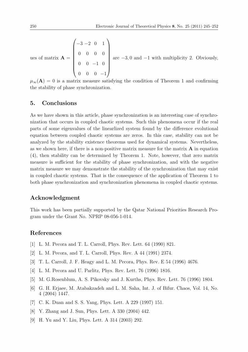
250 Electronic Journal of Theoretical Physics 8, No. 25 (2011) 245–252
ues of matrix A =
⎛⎜⎜⎜⎜⎜⎜⎜⎝
−3 −2 0 1
0 0 0 0
0 0 −1 0
0 0 0 −1
⎞⎟⎟⎟⎟⎟⎟⎟⎠are −3, 0 and −1 with multiplicity 2. Obviously,
μ∞(A) = 0 is a matrix measure satisfying the condition of Theorem 1 and confirming
the stability of phase synchronization.
5. Conclusions
As we have shown in this article, phase synchronization is an interesting case of synchro-
nization that occurs in coupled chaotic systems. Such this phenomena occur if the real
parts of some eigenvalues of the linearlized system found by the difference evolutional
equation between coupled chaotic systems are zeros. In this case, stability can not be
analyzed by the stability existence theorems used for dynamical systems. Nevertheless,
as we shown here, if there is a non-positive matrix measure for the matrix A in equation
(4), then stability can be determined by Theorem 1. Note, however, that zero matrix
measure is sufficient for the stability of phase synchronization, and with the negative
matrix measure we may demonstrate the stability of the synchronization that may exist
in coupled chaotic systems. That is the consequence of the application of Theorem 1 to
both phase synchronization and synchronization phenomena in coupled chaotic systems.
Acknowledgment
This work has been partially supported by the Qatar National Priorities Research Pro-
gram under the Grant No. NPRP 08-056-1-014.
References
[1] L. M. Pecora and T. L. Carroll, Phys. Rev. Lett. 64 (1990) 821.
[2] L. M. Pecora, and T. L. Carroll, Phys. Rev. A 44 (1991) 2374.
[3] T. L. Carroll, J. F. Heagy and L. M. Pecora, Phys. Rev. E 54 (1996) 4676.
[4] L. M. Pecora and U. Parlitz, Phys. Rev. Lett. 76 (1996) 1816.
[5] M. G.Rosenblum, A. S. Pikovsky and J. Kurths, Phys. Rev. Lett. 76 (1996) 1804.
[6] G. H. Erjaee, M. Atabakzadeh and L. M. Saha, Int. J. of Bifur. Chaos, Vol. 14, No.4 (2004) 1447.
[7] C. K. Duan and S. S. Yang, Phys. Lett. A 229 (1997) 151.
[8] Y. Zhang and J. Sun, Phys. Lett. A 330 (2004) 442.
[9] H. Yu and Y. Liu, Phys. Lett. A 314 (2003) 292.

Electronic Journal of Theoretical Physics 8, No. 25 (2011) 245–252 251
[10] C. Zhou and C. H. Lai, Phys. Rev. E 58 (1998) 5185.
[11] H. G. Schuster, Handbook of Chaos Control, WileyVCH, 1999.
[12] A. Pikovsky, M. Rosenblum and J. Kurths, Synchronization a Universal Concept inNonlinear Sciences, Cambridge Univ. Press, Cambridge, UK, 2001.
[13] E. W. Bai and K. E. Lonngsen, Chaos Solitons Fractals 8 (1997) 51.
[14] H. Zhang and X. K. Ma, Chaos Solitons Fractals 21 (2004) 39.
[15] S. Codreanu, Chaos Solitons Fractals 15 (2003) 507.
[16] M. T. Yassen, Chaos, Solitons Fractals 23 (2005) 131.
[17] M. C. Ho, Y. C. Hung and C. H. Chou, Phys. Lett. A 296 (2002) 43.
[18] M. Ali and J. Q. Fang, Phys. Rev. E 55 (1997) 5285.
[19] G. H. Erjaee, Chaos Solitons Fractals 39 (2000) 1195.
[20] K. Sun and J. C. Sprott, EJTP 6, No. 22 (2009) 123-134


EJTP 8, No. 25 (2011) 253–266 Electronic Journal of Theoretical Physics
Synchronization of Different ChaoticFractional-Order Systems via Approached
Auxiliary System the Modified Chua Oscillator andthe Modified Van der Pol-Duffing Oscillator
T. Menacer∗ and N. Hamri†
Department of Mathematics University Mentouri Constantine, Algeria
Received 6 November 2010, Accepted 16 March 2011, Published 25 May 2011
Abstract: In this paper we propose the study of synchronization between two different
chaotic fractional-order systems via approached auxiliary system, we choose the modified Chua
oscillators as a master system and the modified Van der Pol-Duffing oscillator (MVDPD) as a
slave system, this method is also detected for both well known systems Chen and Lu. Routh-
Hurwitz criterion is used for the study of stability of error system between the master-slave
systems. Numerical results show the effectiveness of the theoretical analysis.c© Electronic Journal of Theoretical Physics. All rights reserved.
Keywords: Chaos; Chaotic Fractional-Order System, Auxiliary System; Synchronization; Routch
–Hurwitz Criterion
PACS (2010): 05.45.Pq; 05.45.Xt; 05.45.-a
1. Introduction
In recent years considerable interest is assigned to the applications of fractional derivatives
(of fractional order) in several areas. It has been found in the interdisciplinary fields, many
systems can be described by Fractional differential equations. Recently, synchronization
of fractional order chaotic systems is starting to attract increasing attention due to its
potential applications in secure communications and process control [2].
During this decade, several types of synchronization (complete synchronization or
identical generalized phase, projective) [12] have been studied and many methods have
been proposed, but all these types and methods are encompassed in two modes of syn-
chronization. The first method is based on a mutual coupling between two or more chaotic

254 Electronic Journal of Theoretical Physics 8, No. 25 (2011) 253–266
systems. The second is called master or slave-way coupling: Its principle is to choose a
generator of chaos called ”transmitter”. The latter is described by equations recurring
and characterized by its state variables constituting the state vector. Some components
of this vector are transmitted to a second system, called ”receiver”. This paper will look
at the second mode, and we chose the systems of Van der Pol-Duffing modified (MVDPD)
and the system of Chua modified and we try to study the synchronization of both systems
then those of Chen and LU using the criterion of Routh-Hurwitz generalized to fractional
order to study the stabilization of error system.
Fractional calculus is a generalization of ordinary differentiation and integration to
arbitrary order but there are several definitions of fractional derivatives. In this paper,
we use the Caputo-type fractional derivative defined in [10] by:
Dqf(t) = 1Γ(n−q)
∫ t
0(t− τ)n−q−1f (n)(τ)dτ = jn−q( dn
dtnf(t))
Where n = [q]the value of is q rounded up to the nearest integer, Γis the gamma function.
For the numerical solutions of the systems that we study, we use the Adams-Bash
forth-Moulton predictor-corrector scheme [4].
2. Systems Description
The first system in which we are interested is the Van der pol-Duffing oscillator (MVDPD)
which is an improved model of an autonomous chaotic system by King and Gaito in 1992
[14], in this paper we will be interested in playing fractional version of the system.
While the second is derived from the famous Chua’s circuit [15-17] in fact, it is now
obvious that both oscillators can be represented by the simplified and generic electrical
circuit of Fig.1, The difference in their qualitative dynamical behaviour lies only on the
physical realization of the nonlinear resistance (N), and of course on the parameters
selection.
Fig. 1 The electrical model of the MVDPD oscillator.

Electronic Journal of Theoretical Physics 8, No. 25 (2011) 253–266 255
Fig. 2 (a) The physical realization of the nonlinear resistance and (b) the normal Chua oscillator.
2.1 The Fractional –Order (MVDPD) System
The fractional –order (MVDPD) system is given as follows:⎧⎪⎪⎪⎪⎨⎪⎪⎪⎪⎩dqxdtq
= m(y − x3 + αx+ μ)
dqydtq
= x− y − z
dqzdtq
= βy − γz
(1)
• That since the parameter μ is in general cancelled with the offset current of the
op-amp; we further cancel it from our equations.
• Where q is the fractional order satisfying q ∈ (0, 1], the parameters β,m, γ and α
are all positive real, where q = 1, system (1) is the original integer-order (MVDPD)
system exhibits chaotic behaviours with the parameter values
β = 200,m = 100,γ= 0.2 and α= 0.1
• To evaluate equilibrium points, let
dqx
dtq= 0,
dqy
dtq= 0 and
dqz
dtq= 0
Then E0(0, 0, 0),E+(x+,y+,z+), E−(x−,y−,z−)Are the equilibrium points of system (1)
Where:
x+ = 1β
β+γβ3+γ3+3βγ2+3β2γ
√αβ6 + β5γ + 4αβ5γ + β2γ4 + 3β3γ3 + 3β4γ2 + αβ2γ4 + 4αβ3γ3 + 6αβ4γ2
y+ = 1β
γβ3+γ3+3βγ2+3β2γ
√αβ6 + β5γ + 4αβ5γ + β2γ4 + 3β3γ3 + 3β4γ2 + αβ2γ4 + 4αβ3γ3 + 6αβ4γ2
z+ = 1β3+γ3+3βγ2+3β2γ
√αβ6 + β5γ + 4αβ5γ + β2γ4 + 3β3γ3 + 3β4γ2 + αβ2γ4 + 4αβ3γ3 + 6αβ4γ2
Using the parameter values:
m = 100 , β=200 , γ=0.2 and α=0.1 The system (1) has tree point’s equilibrium

256 Electronic Journal of Theoretical Physics 8, No. 25 (2011) 253–266
E0(0, 0, 0), E+(0.3178, 3, 1749× 10−0.4, 0.31749)
and
E−(−0.3178,−3, 1749× 10−0.4,−0.31749)And their eigenvalues are given as:
E0(0, 0, 0)...λ1 = 13.436, λ2,3 = -2.318± 12.046i
E+(0.3178, 3.1749× 10−0.4, 0.31749)...λ1 = −23.515, λ2,3 = 1.0081± 13.075i
E−(−0.3178,−3.1749× 10−0.4,−0.31749)...λ1 = −23.515, λ2,3 = 1.0081± 13.075i
But
for the stability analysis we have this theorem introduced in [21].
Theorem 1
The following autonomous system:
Dqx = Ax. x(0)=x0
with 0 ≺ q ≺ 1, x ∈ Rn and A ∈ Rn × Rn
Is asymptotically stable if and only if |arg(λ)| qπ/2
Is satisfied for all eigenvalues (λ)of matrix A.Also, this system is stable if and
only if |arg(λ)| ≥ qπ/2is satisfied for all eigenvalues of matrix A and those critical
eigenvalues which satisfy |arg(λ)| = qπ/2
Have geometric multiplicity one.
Fig.3 shows stable and unstable regions according to the above theorem.
Fig. 3 Stability region of the fractional-order system.
• The equilibrium point E0(0, 0, 0)is a saddle point
of index 1[3], however, the equilibrium points E+ and E−are saddle points of index 2 [3].
Thus, by the theorem 1 the necessary condition for the fractional-order (MAVPD)
system (1) to remain chaotic is
q 2
πarctan(
|Im(λ2,3|Reλ2,3
)

Electronic Journal of Theoretical Physics 8, No. 25 (2011) 253–266 257
(a) The system is chaotic for q = 0.98. (b) Its stable for q = 0.94
Fig. 4
Consequently, the lowest fractional order q for which the fractional-order (MAVPD) sys-
tem (1) demonstrates chaos using the above mentioned parameters is given by the in-
equality q 0.95146.
Fig 4 shows the system (1) is chaotic for α = 0.98 and is stable for q = 0.94
2.2 The Fractional-Order Chua System
Our second model is derived from the well-known and famous Chua’s circuit[17] where the
nonlinear element(commonly called Chua’s diode) is implemented using two diodes only,
in addition to an op-amp and some resistors (see Fig.3(b) for an example), Several other
practical implementations of a Chua’s diode characterized by a five-segments piecewise-
linear current-voltage characteristic have been proposed [16].An implementation of Chua’s
circuit with a cubic nonlinearity was first described by Zhong[17].The advantage of the
cubic nonlinearity are that it requires no absolute-valued functions, it is smooth and
thus more suitable for mathematical calculations. Physically, the original Chua’s circuit
does not involve any resistor in series with the inductor. This resistor appears in the
Chua oscillator of Ref.[18]. Coming back to the model of Fig.2 (b), we now rename the
circuit elements by introducing an index “c” on them, and taking the current-voltage
characteristics of the nonlinear resistance in the form:
i(V ) = νc + a2V + b2V3.
Therefore, it is obvious that the Chua’s oscillator will also be described by a set of first-
order coupled differential equations similar to those of (MAVPD) system.
One can therefore conclude that the MAVPD and the modified Chua oscillators are
in fact the same model, with their specific qualitative dynamical behaviour depending
Only on the selection of their parameters, since an inductor can always be physi-
cally constructed with a lower (and negligible) series resistance, and because we need to
stay closer to the original Chua circuit oscillator can thus be described by the following

258 Electronic Journal of Theoretical Physics 8, No. 25 (2011) 253–266
equations: ⎧⎪⎪⎪⎪⎨⎪⎪⎪⎪⎩·x = η(y − x3 + μx),·y = x− y − z,
·z = ρy,
(2)
Where the parameters η, μ and ρ are all positive real
In order to obtain the so-called double scroll attractor which is specific to the family
of Chua’s circuits, we use the same selection of parameters as in [18], that is η = 10, ρ =
16 and μ = 0.143.
2.3 Fractional Version of Modified Chua’s System
The fractional –order Chua system is given as follows:⎧⎪⎪⎪⎪⎨⎪⎪⎪⎪⎩dqxdtq
= η(y − x3 + μx)
dqydtq
= x− y − z
dqzdtq
= ρy
(3)
Where q is the fractional order satisfying q ∈ (0, 1], the parameters ρ, η, and μ are all
positive real, where q = 1, system (3) is the original integer-order Chua system exhibits
chaotic behaviors with the parameter values ρ = 16, η = 10, and μ= 0.143
The system (2) has tree point’s equilibrium given by:
E0(0, 0, 0), E+(√μ, 0,
√μ) andE−(−
√μ, 0, -
√μ)
Using the parameter values:
ρ = 16 , η=10 , and μ=0.143 the points equilibrium are given by:
E0(0, 0, 0) , E+(0.37815, 0, 0.37815) and E−(-0.37815, 0,-0.37815) And their eigenval-ues are given as:
E0(0, 0, 0)...λ1 = 14.889, λ2,3 = −0.79474± 3.8386i
E+(0.37815, 3.0, 0.37815)...λ1 = −4.2846, λ2,3 = 0.21236± 3.2611i
E−(−0.37815, 3.0,−0.37815)... λ1 = −4.2846, λ2,3 = 0.21236± 3.2611i
• The equilibrium point E0(0, 0, 0) is a saddle point
of index 1,however, the equilibrium points E+ and E− are saddle points of index 2
Thus, by the theorem 1 the necessary condition for the fractional-order (Chua) system
(3) to remain chaotic is
q 2
πarctan(
|Im(λ2,3|Reλ2,3
)
Electronic Journal of Theoretical Physics 8, No. 25 (2011) 253–266 259
Consequently, the lowest fractional order q for which the fractional-order (Chua) system
(3) demonstrates chaos using the above mentioned parameters is given by the inequality
q 0.9591.
Fig 5 shows the system (3) is chaotic for q = 0.98 and is stable for q = 0.94
3. Synchronization of two Different Chaotic Fractional Systems
with Auxiliary System
In this study we will study the synchronization between two different fractional systems
with auxiliary system
3.1 The Method of Auxiliary System Approach
The principle of this method is based on the fact that even if the sending system
x(t)conducted two identical receptor systems y(t) and z(t) starting with different ini-
tial conditions in the attraction basin, then the Stability analysis of synchronization in
the space X ⊕ Y , which may generally have a very complicated shape y(t) = φ(x(t)),
may be replaced by the stability analysis is quite simple z(t) = y(t)in the space Z ⊕ Y
For this purpose we assume the following driver, slave and auxiliary system
xq = F (x(t)) (4)
yq = G(y(t), g, x(t)) (5)
And auxiliary system
zq = G(z(t), g, x(t)) (6)
Which is identical to the receiving system(5), Clearly, when the system receiver (5) and
his auxiliary (6) have same transmission signal x(t), then the fields vector in phase space
of the receiver and auxiliary system are identical and the systems can grow on identical
attractors.
It is easy to show that the linear stability of the manifold z(t) = y(t) is equivalent to
the linear stability of manifold of synchronized movements in X⊕Y which is determined
by φ(.).the linear zed equations that govern the evolution of the quantities
ζy(t) = y(t)− φ(x(t))and ζz(t) = z(t)− φ(x(t))
Are
ζqy(t) = DG(φ(x(t), g, x(t))× ζy(t)
ζqz (t) = DG(φ(x(t), g, x(t))× ζz(t)
With DG(w, hu(t)) =∂G(w,hu(t)
∂w
Since the linear zed equations for ζy(t) et ζz(t) are identical, linear zed equations for
ζz(t) − ζy(t) = z(t) − y(t) have the same Tacobian matrix DG(., g, x(t)) in the previous
equation.
260 Electronic Journal of Theoretical Physics 8, No. 25 (2011) 253–266
So, if the collector synchronized movements inX⊕Y ⊕Zis linearly stable forz(t)−y(t),then it is linearly stable for ζy(t) = y(t)− φ(x(t)) and vice versa
The study of synchronization goes back to the study of stability in the vicinity of the
origin of a new system that gives it the name of “system error”. The latter represents
the disturbance that may exist between the transmitting and receiving system.
To study the stability of the system error we will use the criterion of Routh-Hurwitz
generalized to fractional order [1]
3.2 Some Stability Conditions
Let (xe, ye, ze)be an equilibrium solution of the following three dimensional fractional-
order systems: ⎧⎪⎪⎪⎪⎨⎪⎪⎪⎪⎩dqx(t)dtq
= f(x, y, z)
dqy(t)dtq
= g(x, y, z)
dqz(t)dtq
= h(x, y, z)
(7)
Where q ∈ (0, 1].the eigenvalues equation of the equilibrium point (xe, ye, ze) is given by
the following polynomial:P (λ) = λ3 + a1λ2 + a2λ+ a3 = 0
And its discriminant D (P) is given as:
D(P ) = 18a1a2a3 + (a1a2)2 − 4a3(a1)
3 − 4(a2)3 − 27(a3)
2
(1) If D(P ) 0, then the necessary and sufficient condition for the equilibrium point
(xe, ye, ze), to be locally asymptotically stable, is :
a1 0, a2 0, a1a2−a3 0.
(2) If D(P ) ≺ 0, a1 0, a2 0, a3 0. then (xe, ye, ze) is locally asymptotically stable
for,q ≺ 2/3, However, if D(P ) ≺ 0, a1 ≺ 0, a2 ≺ 0 , q 2/3, then all roots of
equation satisfy the condition |arg(λ)| ≺ qπ/2.
(3) if D(P ) ≺ 0, a1 0, a2 0,a1a2 − a3 = 0. then (xe, ye, ze) is locally asymptotically
stable for all q ∈ (0, 1).(4) the necessary condition for the equilibrium point (xe, ye, ze) To be locally asymptot-
ically stable, is a3 0
Synchronization of Modified Chua’s System and MAVPD System
Let us take in this paragraph the two preceding studies, the first is the fractional modi-
fied Chua system, the second is the fractional MAVPD system and we will detect their
synchronization with an auxiliary system.

Electronic Journal of Theoretical Physics 8, No. 25 (2011) 253–266 261
For this we assume the modified Chua system as transmitter (master):⎧⎪⎪⎪⎪⎨⎪⎪⎪⎪⎩dqx1
dtq= η(y1 − x31 + μx1)
dqy1dtq
= x1 − y1 − z1
dqz1dtq
= ρy1
(8)
And the MAVPD system as receiving (slave).⎧⎪⎪⎪⎪⎨⎪⎪⎪⎪⎩dqx2
dtq= m(y2 − x32 + αx2)− k(x2 − x1)
dqy2dtq
= x2 − y2 − z2
dqz2dtq
= βy2 − γz2
..............(9) (9)
The master system is coupled with the slave system only by the x(t) scalar
We choose the auxiliary system that is identical to the slave system (9) (witch different
initial conditions). ⎧⎪⎪⎪⎪⎨⎪⎪⎪⎪⎩dqx3
dtq= m(y3 − x3 + αx3)− k(x3 − x1)
dqy3dtq
= x3 − y3 − z3
dqz3dtq
= βy3 − γz3
(10)
Subtraction of the two systems (9) and (10), gives us the following error system:⎧⎪⎪⎪⎪⎨⎪⎪⎪⎪⎩dqe1dtq
= (mα− k)e1 +me2 −m(x33 − x32)
dqe2dtq
= e1 − e2 − e3
dqe3dtq
= βe2 − γe3
(11)
Where e1 = x3 − x2, e2= y3−y2, e3= z3−z2The system (11) can be written as following matrix:
⎛⎜⎜⎜⎜⎝dqe1dtq
dqe2dtq
dqe3dtq
⎞⎟⎟⎟⎟⎠ = A
⎛⎜⎜⎜⎜⎝e1
e2
e3
⎞⎟⎟⎟⎟⎠+ φ(x, y, z)(12)
Where A
⎛⎜⎜⎜⎜⎝mα− k m 0
1 -1 -1
0 β γ
⎞⎟⎟⎟⎟⎠
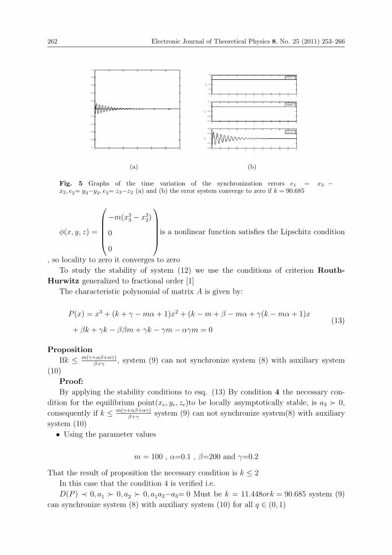
262 Electronic Journal of Theoretical Physics 8, No. 25 (2011) 253–266
(a) (b)
Fig. 5 Graphs of the time variation of the synchronization errors e1 = x3 −x2, e2= y3−y2, e3= z3−z2 (a) and (b) the error system converge to zero if k = 90.685
φ(x, y, z) =
⎛⎜⎜⎜⎜⎝−m(x33 − x32)
0
0
⎞⎟⎟⎟⎟⎠is a nonlinear function satisfies the Lipschitz condition, so locality to zero it converges to zero
To study the stability of system (12) we use the conditions of criterion Routh-
Hurwitz generalized to fractional order [1]
The characteristic polynomial of matrix A is given by:
P (x) = x3 + (k + γ −mα + 1)x2 + (k −m+ β −mα + γ(k −mα + 1)x
+ βk + γk − ββm+ γk − γm− αγm = 0(13)
Proposition
Ifk ≤ m(γ+αβ+αγ)β+γ
, system (9) can not synchronize system (8) with auxiliary system
(10)
Proof:
By applying the stability conditions to esq. (13) By condition 4 the necessary con-
dition for the equilibrium point(xe, ye, ze)to be locally asymptotically stable, is a3 0,
consequently if k ≤ m(γ+αβ+αγ)β+γ
system (9) can not synchronize system(8) with auxiliary
system (10)
• Using the parameter values
m = 100 , α=0.1 , β=200 and γ=0.2
That the result of proposition the necessary condition is k ≤ 2
In this case that the condition 4 is verified i.e.
D(P ) ≺ 0, a1 0, a2 0, a1a2−a3= 0 Must be k = 11.448ork = 90.685 system (9)
can synchronize system (8) with auxiliary system (10) for all q ∈ (0, 1)

Electronic Journal of Theoretical Physics 8, No. 25 (2011) 253–266 263
(a) (b) (c)
Fig. 6 Graphs of the time variation of the synchronization errors e1 = x3 −x2, e2= y3−y2, e3= z3−z2 (a) and (b) the error system converge to zero if k = 22 (c) the errorsystem is instable if k = 2
Synchronization of Fractional Chen System and Fractional LU
System
In this paragraph we replied this method of synchronization for two well known systems,
the first is frictional Chen system and the second is fractional Lu system with auxiliary
system
For this we assume the fractional Chen system as transmitter (master):
⎧⎪⎪⎪⎪⎨⎪⎪⎪⎪⎩dqx1
dtq = a(y1 − x1),
dqy1
dtq = (c− a)y1 − x1z1 + cy1,
dqz1
dtq = x1y1 − bz1,
(14)
Where (a, b, c) = (35, 3, 28) Consequently, the lowest fractional order qfor which the
fractional-order Chen system (14) demonstrates chaos using the above mentioned param-
eters is given by the inequality.q 0.82
And we assume the fractional Lu system as receiving (slave).
⎧⎪⎪⎪⎪⎨⎪⎪⎪⎪⎩dqx2
dtq= α(y2 − x2),
dqy2dtq
= δy2 − x2z2 − k(y2 − y1),
dqz2dtq
= x2y2 − βz2,
(15)
(α, β, δ) = (36, 3, 20) and k is coupling parameter Consequently, the lowest fractional
order q for which the fractional-order LU system (15) demonstrates chaos using the above
mentioned parameters is given by the inequality.q 0.91605
The master system is coupled with the slave system only by the y(t) scalar
We choose the auxiliary system that is identical to the slave system (15) (with different
initial conditions).
264 Electronic Journal of Theoretical Physics 8, No. 25 (2011) 253–266
⎧⎪⎪⎪⎪⎨⎪⎪⎪⎪⎩dqx3
dtq= α(y3 − x3),
dqy3dtq
= δy3 − x3z3 − k(y3 − y1),
dqz3dtq
= x3y3 − βz3,
(16)
Subtraction of the two systems (16) and (15), gives us the following error system⎧⎪⎪⎪⎪⎨⎪⎪⎪⎪⎩dqe1dtq
= α(e2 − e1)
dqe2dtq
= βe2 − ke2 − x3e1 − z2e1
dqe3dtq
= x3e2 − y2e1 − αe3
(17)
Where e1 = x3 − x2, e2= y3−y2, e3= z3−z2The system (17) can be written as following matrix:
⎛⎜⎜⎜⎜⎝dqe1dtq
dqe2dtq
dqe3dtq
⎞⎟⎟⎟⎟⎠ = A
⎛⎜⎜⎜⎜⎝e1
e2
e3
⎞⎟⎟⎟⎟⎠+ φ(x, y, z)(18)
Where A
⎛⎜⎜⎜⎜⎝−α α 0
0 δ-k 0
0 0 -β
⎞⎟⎟⎟⎟⎠
φ(x, y, z) =
⎛⎜⎜⎜⎜⎝0
−z2e1 − x3e1
x3e2 − y2e1
⎞⎟⎟⎟⎟⎠is a nonlinear function satisfies the Lipschitz condition,so locality to zero it converges to zero
The characteristic polynomial of matrix A is given by
x3 + (k+α+β−δ)x2 + (−α(−k+δ)+β(k+α−δ))x−αβ(−k+δ) (19)
• By applying the stability conditions to esq.(19) with condition 4 the necessary con-
dition for the equilibrium point (xe, ye, ze) to be locally asymptotically stable, is
a3 0, consequently if k ≺ δ system (14) can not synchronize system (15) with
auxiliary system (16)
• . Using the parameter values(α, β, δ) = (36, 3, 20)
According to the previous result, the necessary condition for synchronization is achieved
k ≥ 21
Figure (6) show the synchronization is realized in case k = 22 but not realized in case
k = 2
Electronic Journal of Theoretical Physics 8, No. 25 (2011) 253–266 265
Conclusion
In this paper we have studied the synchronization between different chaotic fractional
–order systems, with the auxiliary system, we have applied this method on both systems:
The modified Chua oscillator as transmitter system and Van der Pol-Duffing modified
(MVDPD) as receiver system; we have also used it again on two well know systems Chen
and LU.Using the criterion of routh Hurwitz to study the stability of the system error.
Numerical results show the effectiveness of the theoretical analysis.
References
[1] E. Ahmed, A.M.A. El-Sayed, Hala A.A. El Saka On some Routh. Hurwitz conditionsfor fractional order dierential equations an their applications in orenz,Rosler,.Chuaand Chen systems. Phys Lett A.2006; 358:1.4
[2] Ahmad M. Harb, Wajdi M. Ahmad ”Chaotic systems synchronization in securecommunication.systems.”.in compting,2006:169-177.
[3] Tavazoei MS, Haeri M.A necessary condition for double scroll attractor existence Infractional-order.systems.Phys Lett A 2007;367:102.13.
[4] Kai Diethelm and Alan D.Freed”The FracPECE Subroutine for the NumericalSolution of Differential Equations of Fractional Order” Gottingen, Gesellschaft furwissenschaftliche. Dataverarbeitung, 1999, pp. 57-71
[5] Poludbny, I”, fractional differential equations “Mathematics in Science andEngineering, 198, Academic press, (1999)
[6] Hilaire Fotsin, Samuel Bowing, and Jamel Daafouz: ”Adaptive synchro nizationof two chaotic systems.consisting of modi.ed Van der Pol-Du ng and Chuaoscillations”.Chaos, Solitons and Fractals 26 (2005).215.229
[7] Matouk AE, Agiza HN. Bifurcations, chaos and synchronization in ADVP circuitwith parallel resistor.J Math Anal Appl 2008;341:259.69.
[8] M.Lakshmman, K.Murali, Chaos in Nonlinear Oscillators: Controlling andSynchronization, World Scientific, 1996
[9] Caputo, “Linear model of dissipation whose Q is almost frequency indepondent”-II.Geophys, J.R Astr, Soc, vol 13, 1967, p, p, 529-539
[10] Caputo M. “Linear models of dissipation whose Q is almost frequency independent-II.” Geophys J R Astron Soc 1967; 13:529–39.
[11] JunwelWang, Xiong, Yanbin Zhang ”Extending synchronization scheme to chaoticfractional-order.Chen systems”.Physica A 370 (2000) 279-265.
[12] Wang Xingyuan, HeYijie ”Projective synchronization of fractional order chaoticsystem based on.linear separation” .Physica Letters A 372.(2008)435-441.
[13] King GP, Gaito ST, Bistable chaos, I, Unfolding the cusp.phys Rev A 1992; 46;3093-599
[14] King GP, Gaito ST. Bistable chaos. I. Unfolding the cusp. Phys Rev A 1992; 46:3093–599.
[15] Hwang CC, Chow H-Y, Wang Y-K. A new feedback control of a modified Chua scircuit system. Physical D 1996; 92:95–100.

266 Electronic Journal of Theoretical Physics 8, No. 25 (2011) 253–266
[16] Matsumoto T. A chaotic attractor from Chua s circuit. IEEE Trans Circ Syst 1984;31:1055–8.
[17] Zhong GQ. Implementation of Chua s circuit with a cubic nonlinearity. Int J BifurChaos 1994; 41:934–41.
[18] Madam RN. Chua s circuit: a paradigm for chaos. Singapore: World Scientific; 1993.
[19] Jiang G-P, Zheng WX, Chen G. Global chaos synchronization with channel time-delay. Chaos, Solutions & Fractals 2004; 20:267–75.
[20] A.E Matouk ”Chaos, feedback control and synchronization of a frac- tional Ordermodi.ed Autonomous.Van der Pol.Du ng circuit” Commun nonlinear Sci NumerSimulat xxx (2010) xxx.xxx. (article in prese).
[21] D.Matignon, Stability result on fractional differential equations with applications tocontrol processing. In: IMACS-SMC proceding, Lille, France.1996, pp.963-968

EJTP 8, No. 25 (2011) 267–272 Electronic Journal of Theoretical Physics
A Universal Nonlinear Control Law for theSynchronization of Arbitrary 4-D
Continuous-Time Quadratic Systems
Zeraoulia Elhadj∗1 and J. C. Sprott†2
1Department of Mathematics, University of Tebessa, (12002), Algeria2Department of Physics, University of Wisconsin, Madison, WI 53706, USA
Received 6 July 2010, Accepted 10 February 2011, Published 25 May 2011
Abstract: In this letter we show the existence of a universal nonlinear control law (without
any conditions) for the synchronization of arbitrary 4-D continuous-time quadratic systems.c© Electronic Journal of Theoretical Physics. All rights reserved.
Keywords: Synchronization; Universal Nonlinear Control Law; 4-D Continuous-Time Quadratic
Systems
PACS (2010): 05.45.Pq; 05.45.Xt; 05.45.-a
1. Introduction
There are several methods of chaos synchronization. For example in [9], a method is
introduced to synchronize two identical chaotic systems with different initial conditions.
An adaptive control approach is presented in [10], a backstepping design is given in [13],
an active control method is presented in [5-11,12], and a nonlinear control scheme is
given in [4,6,8]. In fact, there are many applications of chaos synchronization in phys-
ical, chemical, and ecological systems, and in secure communications [1,2,3,7,9,10]. For
4-D continuous-time quadratic systems, some of these methods were applied to Lorenz-
Stenflo systems, Qi systems, and other hyperchaotic quadratic systems as shown in
[14,15,16,17,18,19,20]. In this letter, we apply nonlinear control theory to synchronize
∗ [email protected] and [email protected]† [email protected]
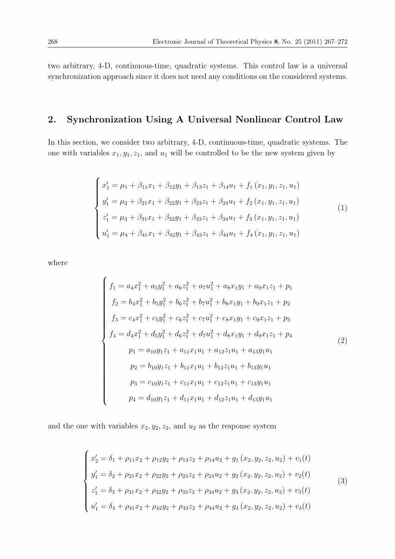
268 Electronic Journal of Theoretical Physics 8, No. 25 (2011) 267–272
two arbitrary, 4-D, continuous-time, quadratic systems. This control law is a universal
synchronization approach since it does not need any conditions on the considered systems.
2. Synchronization Using A Universal Nonlinear Control Law
In this section, we consider two arbitrary, 4-D, continuous-time, quadratic systems. The
one with variables x1, y1, z1, and u1 will be controlled to be the new system given by
⎧⎪⎪⎪⎪⎪⎪⎪⎨⎪⎪⎪⎪⎪⎪⎪⎩
x′1 = μ1 + β11x1 + β12y1 + β13z1 + β14u1 + f1 (x1, y1, z1, u1)
y′1 = μ2 + β21x1 + β22y1 + β23z1 + β24u1 + f2 (x1, y1, z1, u1)
z′1 = μ3 + β31x1 + β32y1 + β33z1 + β34u1 + f3 (x1, y1, z1, u1)
u′1 = μ4 + β41x1 + β42y1 + β43z1 + β44u1 + f4 (x1, y1, z1, u1)
(1)
where ⎧⎪⎪⎪⎪⎪⎪⎪⎪⎪⎪⎪⎪⎪⎪⎪⎪⎪⎪⎪⎪⎪⎨⎪⎪⎪⎪⎪⎪⎪⎪⎪⎪⎪⎪⎪⎪⎪⎪⎪⎪⎪⎪⎪⎩
f1 = a4x21 + a5y
21 + a6z
21 + a7u
21 + a8x1y1 + a9x1z1 + p1
f2 = b4x21 + b5y
21 + b6z
21 + b7u
21 + b8x1y1 + b9x1z1 + p2
f3 = c4x21 + c5y
21 + c6z
21 + c7u
21 + c8x1y1 + c9x1z1 + p3
f4 = d4x21 + d5y
21 + d6z
21 + d7u
21 + d8x1y1 + d9x1z1 + p4
p1 = a10y1z1 + a11x1u1 + a12z1u1 + a13y1u1
p2 = b10y1z1 + b11x1u1 + b12z1u1 + b13y1u1
p3 = c10y1z1 + c11x1u1 + c12z1u1 + c13y1u1
p4 = d10y1z1 + d11x1u1 + d12z1u1 + d13y1u1
(2)
and the one with variables x2, y2, z2, and u2 as the response system
⎧⎪⎪⎪⎪⎪⎪⎪⎨⎪⎪⎪⎪⎪⎪⎪⎩
x′2 = δ1 + ρ11x2 + ρ12y2 + ρ13z2 + ρ14u2 + g1 (x2, y2, z2, u2) + v1(t)
y′1 = δ2 + ρ21x2 + ρ22y2 + ρ23z2 + ρ24u2 + g2 (x2, y2, z2, u2) + v2(t)
z′1 = δ3 + ρ31x2 + ρ32y2 + ρ33z2 + ρ34u2 + g3 (x2, y2, z2, u2) + v3(t)
u′1 = δ4 + ρ41x2 + ρ42y2 + ρ43z2 + ρ44u2 + g4 (x2, y2, z2, u2) + v4(t)
(3)

Electronic Journal of Theoretical Physics 8, No. 25 (2011) 267–272 269
where ⎧⎪⎪⎪⎪⎪⎪⎪⎪⎪⎪⎪⎪⎪⎪⎪⎪⎪⎪⎪⎪⎪⎨⎪⎪⎪⎪⎪⎪⎪⎪⎪⎪⎪⎪⎪⎪⎪⎪⎪⎪⎪⎪⎪⎩
g1 = h4x22 + h5y
22 + h6z
22 + h7u
22 + h8x2y2 + h9x2z2 + p5
g2 = m4x22 +m5y
22 +m6z
22 +m7u
22 +m8x2y2 +m9x2z2 + p6
g3 = r4x22 + r5y
22 + r6z
22 + r7u
22 + r8x2y2 + r9x2z2 + p7
g4 = s4x22 + s5y
22 + s6z
22 + s7u
22 + s8x2y2 + s9x2z2 + p8
p5 = h10y2z2 + h11x2u2 + h12z2u2 + h13y2u2
p6 = m10y2z2 +m11x2u2 +m12z2u2 +m13y2u2
p7 = r10y2z2 + r11x2u2 + r12z2u2 + r13y2u2
p8 = s10y2z2 + s11x2u2 + s12z2u2 + s13y2u2
(4)
Here (μi, δi)1≤i≤4 ∈ R8 and (βij, ρij)1≤i,j≤4 ∈ R16 and (ai, bi, ci, di, hi,mi, ri, si)4≤i≤13 ∈ R80
are bifurcation parameters, and v1(t), v2(t), v3(t), and v4(t) are the unknown nonlinear
controller such that two systems (1)-(2) and (3)-(4) can be synchronized.
First, let us define the following quantities depending on the above two systems:⎧⎪⎪⎪⎪⎪⎪⎪⎪⎪⎪⎪⎪⎪⎪⎪⎪⎪⎪⎪⎪⎪⎨⎪⎪⎪⎪⎪⎪⎪⎪⎪⎪⎪⎪⎪⎪⎪⎪⎪⎪⎪⎪⎪⎩
η1 = h7u21 − a9u1x2 + h13u1y2 − a12u1z2 + ρ14u1 − a7u
22 + h9u2x1
η2 = −a13u2y1 + h12u2z1 − β14u2 + h4x21 + h8x1y2 + h9x1z2 + ρ11x1
η3 = −a4x22 − a8x2y1 − a9x2z1 − β11x2 + h5y21 + h10y1z2 + ρ12y1 − a5y
22
η4 = −a10y2z1 − β12y2 + h6z21 + ρ13z1 − a6z
22 − β13z2 − μ1 + δ1
η5 = m7u21 − b9u1x2 +m13u1y2 − b12u1z2 + ρ24u1 − b7u
22 +m9u2x1
η6 = −b13u2y1 +m12u2z1 − β14u2 +m4x21 +m8x1y2 +m9x1z2 + ρ21x1
η7 = −b4x22 − b8x2y1 − b9x2z1 − β21x2 +m5y21 +m10y1z2 + ρ22y1 − b5y
22
η8 = −b10y2z1 − β22y2 +m6z21 + ρ23z1 − b6z
22 − β23z2 − μ2 + δ2
(5)
⎧⎪⎪⎪⎪⎪⎪⎪⎪⎪⎪⎪⎪⎪⎪⎪⎪⎪⎪⎪⎪⎪⎨⎪⎪⎪⎪⎪⎪⎪⎪⎪⎪⎪⎪⎪⎪⎪⎪⎪⎪⎪⎪⎪⎩
η9 = r7u21 − c9u1x2 + r13u1y2 − c12u1z2 + ρ34u1 − c7u
22 + r9u2x1
η10 = −c13u2y1 + r12u2z1 − β34u2 + r4x21 + r8x1y2 + r9x1z2 + ρ11x1
η11 = −c4x22 − c8x2y1 − c9x2z1 − β31x2 + r5y21 + r10y1z2 + ρ32y1 − c5y
22
η12 = −c10y2z1 − β32y2 + r6z21 + ρ33z1 − c6z
22 − β33z2 − μ3 + δ3
η13 = s7u21 − d9u1x2 + s13u1y2 − d12u1z2 + ρ44u1 − d7u
22 + s9u2x1
η14 = −d13u2y1 + s12u2z1 − β44u2 + s4x21 + s8x1y2 + s9x1z2 + ρ41x1
η15 = −d4x22 − d8x2y1 − d9x2z1 − β41x2 + s5y21 + s10y1z2 + ρ42y1 − d5y
22
η16 = −d10y2z1 − β42y2 + s6z21 + ρ43z1 − d6z
22 − β43z2 − μ4 + δ4
(6)

270 Electronic Journal of Theoretical Physics 8, No. 25 (2011) 267–272
⎧⎪⎪⎪⎪⎪⎪⎪⎪⎪⎪⎪⎨⎪⎪⎪⎪⎪⎪⎪⎪⎪⎪⎪⎩
ξ1 = β11 + ρ11 + (a4 + h4) (x1 + x2) + a9u1 + a8y1 + a9z1 + h9u2 + h8y2 + h9z2
ξ2 = β12 + ρ12 + (a5 + h5) (y1 + y2) + a10z1 + z2h10
ξ3 = β13 + ρ13 + (a6 + h6) (z1 + z2) + u1a12 + u2h12
ξ4 = β14 + ρ14 + (a7 + h7) (u1 + u2) + y1a13 + y2h13
ξ5 = η1 + η2 + η3 + η4
(7)
⎧⎪⎪⎪⎪⎪⎪⎪⎪⎪⎪⎪⎨⎪⎪⎪⎪⎪⎪⎪⎪⎪⎪⎪⎩
ξ6 = β21 + ρ21 + (b4 +m4) (x1 + x2) + b9u1 + b8y1 + b9z1 +m9u2 +m8y2 +m9z2
ξ7 = β22 + ρ22 + (b5 +m5) (y1 + y2) + b10z1 + z2m10
ξ8 = β23 + ρ23 + (b6 +m6) (z1 + z2) + u1b12 + u2m12
ξ9 = β24 + ρ24 + (b7 +m7) (u1 + u2) + y1b13 + y2m13
ξ10 = η5 + η6 + η7 + η8
(8)
⎧⎪⎪⎪⎪⎪⎪⎪⎪⎪⎪⎪⎨⎪⎪⎪⎪⎪⎪⎪⎪⎪⎪⎪⎩
ξ11 = β31 + ρ31 + (c4 + r4) (x1 + x2) + c9u1 + c8y1 + c9z1 + r9u2 + r8y2 + r9z2
ξ12 = β32 + ρ32 + (c5 + r5) (y1 + y2) + c10z1 + z2r10
ξ13 = β33 + ρ33 + (c6 + r6) (z1 + z2) + u1c12 + u2r12
ξ14 = β34 + ρ34 + (c7 + r7) (u1 + u2) + y1c13 + y2r13
ξ15 = η9 + η10 + η11 + η12
(9)
⎧⎪⎪⎪⎪⎪⎪⎪⎪⎪⎪⎪⎨⎪⎪⎪⎪⎪⎪⎪⎪⎪⎪⎪⎩
ξ16 = β41 + ρ41 + (d4 + s4) (x1 + x2) + d9u1 + d8y1 + d9z1 + s9u2 + s8y2 + s9z2
ξ17 = β42 + ρ42 + (d5 + s5) (y1 + y2) + d10z1 + z2s10
ξ18 = β43 + ρ43 + (d6 + s6) (z1 + z2) + u1d12 + u2s12
ξ19 = β44 + ρ44 + (d7 + s7) (u1 + u2) + y1d13 + y2s13
ξ20 = η13 + η14 + η15 + η16
(10)
Now let the error states be e1 = x2 − x1, e2 = y2 − y1, e3 = z2 − z1, and e4 = u2 − u1.
Then the error system is given by⎧⎪⎪⎪⎪⎪⎪⎪⎨⎪⎪⎪⎪⎪⎪⎪⎩
e′1 = ξ1e1 + ξ2e2 + ξ3e3 + ξ4e4 + ξ5 + v1 (t)
e′2 = ξ6e1 + ξ7e2 + ξ8e3 + ξ9e4 + ξ10 + v2 (t)
e′3 = ξ11e1 + ξ12e2 + ξ13e3 + ξ14e4 + ξ15 + v3 (t)
e′4 = ξ16e1 + ξ17e2 + ξ18e3 + ξ19e4 + ξ20 + v4 (t)
(11)

Electronic Journal of Theoretical Physics 8, No. 25 (2011) 267–272 271
In this letter, we propose the following universal control law for the system (3)-(4):⎧⎪⎪⎪⎪⎪⎪⎪⎨⎪⎪⎪⎪⎪⎪⎪⎩
v1 (t) = − (1 + ξ1) e1 − ξ5
v2 (t) = − (ξ2 + ξ6) e1 − (1 + ξ7) e2 − ξ10
v3 (t) = − (ξ3 + ξ11) e1 − (ξ8 + ξ12) e2 − (1 + ξ13) e3 − ξ15
v4 (t) = − (ξ4 + ξ16) e1 − (ξ9 + ξ17) e2 − (ξ14 + ξ18) e3 − (1 + ξ19) e4 − ξ20
(12)
Then the two 4-D, continuous-time, quadratic systems (1)-(2) and (3)-(4) approach syn-
chronization for any initial condition, since the error system (11) becomes⎧⎪⎪⎪⎪⎪⎪⎪⎨⎪⎪⎪⎪⎪⎪⎪⎩
e′1 = −e1 + ξ2e2 + ξ3e3 + ξ4e4
e′2 = −ξ2e1 − e2 + ξ8e3 + ξ9e4
e′3 = −ξ3e1 − ξ8e2 − e3 + ξ14e4
e′4 = −ξ4e1 − ξ9e2 − ξ14e3 − e4
(13)
and if we consider the Lyapunov function V =e21+e22+e23+e24
2, then it is easy to verify the
asymptotic stability of the error system (13) by Lyapunov stability theory since we havedVdt
= −e21 − e22 − e23 − e24 < 0 for all (μi, δi)1≤i≤4 ∈ R8 and (βij, ρij)1≤i,j≤4 ∈ R16 and
(ai, bi, ci, di, hi,mi, ri, si)4≤i≤13 ∈ R80 and for all initial conditions. If the two systems (1)-
(2) and (3)-(4) are chaotic, then the control law (12) guaranties also their synchronization
for any initial condition. An elementary example of this situation can be found in [14].
Also, we notice that any 4-D, continuous-time, quadratic, chaotic system can be stabilized
(resp. controlled) to a stable 4-D, continuous-time, quadratic system that converges to
an equilibrium point (resp. to a 4-D, continuous-time, quadratic system that converges
to a periodic solution). Furthermore, any 4-D, continuous-time, quadratic system can be
chaotified to a chaotic 4-D, continuous-time, quadratic system.
Conclusion
We have presented a universal nonlinear control law (without any conditions) for the
synchronization of arbitrary 4-D, continuous-time, quadratic systems. This control law
(12) can be considered either as a stabilization, or as a control, or as a chaotification
approach for a general 4-D, continuous-time, quadratic system.
References
[1] A. Pikovsky, M. Rosenblum and J. Kurths, Synchronization, a Universal Concept inNonlinear Science. Cambridge University Press, Cambridge (2001).
[2] E. Mosekilde, Y. Mastrenko and D. Postnov, Chaotic Synchronization. Applicationsfor Living Systems. World Scienctific, Singapore (2002).

272 Electronic Journal of Theoretical Physics 8, No. 25 (2011) 267–272
[3] H. K. Chen, T. N. Lin and J. H. Chen, The stability of chaos synchronization of theJapanese attractors and its application. Jpn. J. Appl. Phys. 42, 2003, 7603–7610.
[4] H. K. Chen, Global chaos synchronization of new chaotic systems via nonlinearcontrol. Chaos, Solitons & Fractals 23, 2005, 1245–1251.
[5] H. K. Chen, Synchronization of two different chaotic systems: A new system andeach of the dynamical systems Lorenz, Chen and Lu. Chaos, Solitons & Fractals 25,2005, 1049–1056.
[6] J. H. Park, Chaos synchronization of a chaotic system via nonlinear control. Chaos,Solitons & Fractals 25, 2005, 579–584.
[7] J. Lu, X. Wu and J. Lu, Synchronization of a unified chaotic system and theapplication in secure communication. Phys. Lett. A 305, 2002, 365–370.
[8] L. Huang, R. Feng and M. Wang, Synchronization of chaotic systems via nonlinearcontrol. Phys. Lett. A 320, 2004, 271–275.
[9] L. M. Pecora and T. L. Carroll, Synchronization in chaotic systems. Phys. Rev. Lett.64, 1990, 821–824.
[10] L. Kocarev and U. Parlitz, General approach for chaotic synchronization withapplication to communication. Phys. Rev. Lett. 74, 1995, 5028–5031.
[11] M. C. Ho and Y. C. Hung, Synchronization two different systems by using generalizedactive control. Phys. Lett. A 301, 2002, 424–428.
[12] M. T. Yassen, Chaos synchronization between two different chaotic systems usingactive control. Chaos, Solitons & Fractals 23, 2005, 131–140.
[13] X. Tan, J. Zhang and Y. Yang, Synchronizing chaotic systems using backsteppingdesign. Chaos, Solitons & Fractals 16, 2003, 37–45.
[14] A. N. Njah and O. D. Sunday, Synchronization of Identical and non-identical 4-D chaotic systems via Lyapunov direct method. International Journal of NonlinearScience, 8 (1), 2009, 3–10.
[15] D. Lu, A. Wang and X. Tian, Control and synchronization of a new hyperchaoticsystem with unknown parameters. Internatinal Journal of Nonlinear Science 6, 2009,224–229.
[16] J. A. Laoye, U. E. Vincent and S. O. Kareem, Chaos control of 4D chaotic systemsusing recursive backstepping nonlinear controller. Chaos, Solitons & Fractals 39, 2009,356–362.
[17] X. Zhang and H. Zhu, Anti-synchronization of two different hyperchaotic systemsvia active and adaptive control. Internatinal Journal of Nonlinear Science 6, 2008,216–223.
[18] U. E. Vincent, Synchronization of identical and non-identical 4-D chaotic systemsvia active control. Chaos, Solitons & Fractals 37, 2008, 1065–1075.
[19] Y. Lei, W. Xu and W. Xie, Synchronization of two chaotic four-dimensional systemsusing active control. Chaos, Solitons & Fractals 32, 2007, 1823–1829.
[20] E. M. Elabbasy, H. N. Agiza and M. M. El-Dessoky, Adaptive synchronization of ahyperchaotic system with uncertain parameter, Chaos, Solitons & Fractals 30, 2006,1133–1142.

EJTP 8, No. 25 (2011) 273–278 Electronic Journal of Theoretical Physics
On a General Class of Solutions of a NonholonomicExtension of Optical Pulse Equation
Pinaki Patra, Arindam Chakraborty1, and A. Roy Chowdhury2∗
1Department of Physics, Swami Vivekananda Institute of Science and Technology,Govindapur , Kolkata - 700150, India
2Department of Physics, Jadavpur University, Kolkata - 700032 , India
Received 23 November 2010, Accepted 10 February 2011, Published 25 May 2011
Abstract: A Nonholonomic extension of an equation obeyed by short pulse in non-linear optics
is obtained.A general class of solutions of such an equation is obtained with the help of Riemann-
Hilbert technique.c© Electronic Journal of Theoretical Physics. All rights reserved.
Keywords: Integrable System; Nonholonomic; Lax Pair; Reimann Hilbert
PACS (2010): 42.65.-k; 05.45.Pq; 05.45.Ac; 05.45.-a
1. Introduction
Recent literature of integrable systems has been enriched by quite a few publications
discussing a new class of systems which are nonholonomic in the sense that they are ac-
companied by differential constraints [1] those cannot be explicitly solved . This actually
enlarges the integrable class itself. People have studied some interesting cases associated
with AKNS [2] systems Kaup-Newell equation and so on . Here in this communication
we have obtained a nonholonomic generalization of a very special type of equation which
governs the propagation of a short optical pulse in nonlinear optics [3]. In the second
part we have shown how a general class of solutions of such an equation can be generated
through the Riemann Hilbert method [6].
∗ (Corresponding author)e-mail: asesh [email protected]

274 Electronic Journal of Theoretical Physics 8, No. 25 (2011) 273–278
2. Formulation
To start with, we consider the Lax pair
ψx = Lψ (1)
ψt =Mψ (2)
L =
⎛⎜⎝−φx 1
−λ φx
⎞⎟⎠ ;N =
⎛⎜⎝A B
C −A
⎞⎟⎠whence consistency leads to
φxt + Ax − C − λB = 0 (3)
Bx + 2A+ 2φxB = 0 (4)
Cx + 2λA− 2φxC = 0 (5)
Next we set
A = a−1λ−1 + a2 + a1λ+ a0λ2 (6)
B = b−1λ−1 + b2 + b1λ+ b0λ2 (7)
C = c−1λ−1 + c2 + c1λ+ c0λ2 (8)
The unknown coefficients are determined in a recursive manner and are given as
a0 = b0 = 0
c0 = η2
a1 = η2φx (9)
b1 = −η2
c1 =1
2η2(φxx + φ2
x
)a2 = −
1
4η2(φxxx − 2φ3
x
)b2 =
1
2η2(φxx − φ2
x
)(10)
c−1 = η1 exp (2φ)
where η1 and η2 are constants .
Along with ;
a−1x = η1 exp (2φ) (11)
b−1xx + 2φxxb−1 + 2φxb−1x + 2η1 exp (2φ) = 0 (12)
c2xx − 2φxxc2 − 2φxc2x + 2η1 exp (2φ) = 0 (13)
and the nonlinear equation ;
φxt + a2x − c2 − b−1 = 0 (14)

Electronic Journal of Theoretical Physics 8, No. 25 (2011) 273–278 275
It is interesting to note that c2 , b−1 are to be determined only as solutions of eq(8)
and eq(9) , which really leads to nonlocal nonholonomic constraints . To proceed further
we consider the special case η1 = 0 , which leads to a−1 = constant ; along with c2 =
η3 exp (2φ) and b−1 = η4 exp (−2φ) so that the nonlinear equations turns out to be ;
φxt = φxxxx − 6φ2xφxx + 2η sinh (2φ) . (15)
by proper choice of ηi. Equation (11) is nothing but the nonlinear equation obeyed by a
short optical pulse propagating in an optical fibre . So, if we assume η1 �= 0 , then eq(10)
can be consider as a nonholonomic generalization of eq (11)5 .
3. General Solutions
To analyze the solutions of the new equation [14] we take recourse to the Riemann-
Hilbert technique [4]. The usual approach is to assume that the analytic wave function
φ(λ) , with the constraint
φ1 (λ)φ2 (λ) = G (λ) (16)
where φ1 , φ2 are the boundary values of φ on the interior and exterior of a close Jordan
curve Γ in the complex λ plane . In case of Riemann - Hilbert problem with simple poles
we assume G (λ) = 1 . Let φ0 be the starting seed solution of eq [14] with ψ0 , the
corresponding Lax eigenfunction [5] . We can set
ψ = χψ0 (17)
If the lax operator corresponding to φ0 be denoted as L0 , then one gets
L = χxχ−1 + χL0χ
−1 (18)
To formulate the Riemann-Hilbert problem we assume that χ contains simple pole in λ
- plane ,
χ =
(1 +
S
λ− λ1
)(19)
along with
χ−1 =(1 +
R
λ− λ1
)(20)
From the condition χχ−1 = 1 one gets
S = −R = (λ1 − μ1)P (21)
where P is the projection operator (P 2 = P ) . Also from Eq.[18] we get
L = L0 − (λ1 − μ1)[P, σ−] (22)

276 Electronic Journal of Theoretical Physics 8, No. 25 (2011) 273–278
The Lax operator has some interesting symmetry property
σ1LTσ1 = L(−φ, λ) (23)
σ2LTσ2 = −L (φ, λ) (24)
with σ1 σ2 being Pauli matrices and σ− = σ1 − iσ2 . An easy seed solution is φ = 0 ,
whence we require the Lax eigenfunction as solution of ;
ψx =
⎛⎜⎝ 0 1
−λ 0
⎞⎟⎠ψ (25)
and ψt =
⎛⎜⎝ η1xλ−1 −η1x2λ−1 − η2λ
η1λ−1 − η1x
2 + η2λ2 −η1xλ−1
⎞⎟⎠ψ (26)
writing out in component form we get one partial differential equation
ψ2t +(−ηx2 + ηλ−1 − λ2
) ψ2x
λ= −ηxλ−1ψ2 (27)
Now it is easy to show that an equation of the form ;
f(x)ωx + g(y)ωy = [δ1(x) + δ2(y)]ω (28)
has a solution of the form
ω = exp
[∫δ1 (x)
f (x)dx+
∫δ2 (y)
g (y)dy
]Θ
(∫1
f (x)dx−
∫1
g (y)dy
)(29)
where Θ is an arbitrary function of its argument. Finally using the explicit of function
δ1 and δ2 from Eqs.[26], we arrive at
ψ1 =μ(θ)√
λ− ηλ−1x2(30)
ψ2 =ηλ−1xμ(θ)√λ− ηλ−1x2
+μx(θ)√
λ− ηλ−1x2(31)
where θ = t + 12aηλ−1 ln
(x+ax−a
), along with a2 = λ3
η. The Projection operator is now
constructed as,
P =| p >< q |< p | q > (32)

Electronic Journal of Theoretical Physics 8, No. 25 (2011) 273–278 277
where | p > and | q > are given by;
| p >=
⎛⎜⎝ a1ψ1(λ1)
a2ψ2(λ1)
⎞⎟⎠ =
⎛⎜⎝u1
u2
⎞⎟⎠ (33)
| q >=
⎛⎜⎝ b1ψ1(μ1)
b2ψ2(μ1)
⎞⎟⎠ =
⎛⎜⎝ v1
v2
⎞⎟⎠ (34)
where Eq.(22) leads to
φx = (λ1 − μ1)u1v2
u1v1 + u2v2(35)
The form of the solution is clearly different from the usual soliton like profile sustained
by original optical pulse equation . The absence of any wavefront (x− vt) suggests that
it is a nonpropagating solution .
Acknowledgement
One of the author (P.P) is grateful to CSIR(Govt. of India) for a Junior Research
Fellowship which made the work possible.
References
[1] A . Karasu , A.Karasu , A . Sakovich , S. Sakovich and R . Turhan - J. Math. Phys.51, 113507(2010)
[2] Ruguang Zhoua, J. Math. Phys. 50, 123502 , 2009
[3] Leblond H , Melnikov I , V Mihalache D - Phys. Rev. Lett. A 78(2008)043802
[4] A . Chakraborty and A. Roy Chowdhury - EJTP . No.24(2010)1− 8
[5] Boris A . Kupershmidt , Phys. Lett. A 372, 2634 (2008)
[6] R. G. Zhou, J. Math. Phys. 36, 4220 (1995)


EJTP 8, No. 25 (2011) 279–286 Electronic Journal of Theoretical Physics
Schwinger Mechanism for Quark-AntiquarkProduction in the Presence of Arbitrary Time
Dependent Chromo-Electric Field
Gouranga C. Nayak∗
C. N. Yang Institute for Theoretical Physics, Stony Brook University, SUNY, StonyBrook, NY 11794-3840, USA
Received 12 November 2010, Accepted 10 February 2011, Published 25 May 2011
Abstract: We study the Schwinger mechanism in QCD in the presence of an arbitrary time-
dependent chromo-electric background field Ea(t) with arbitrary color index a=1,2,...8 in SU(3).
We obtain an exact result for the non-perturbative quark (antiquark) production from an
arbitrary Ea(t) by directly evaluating the path integral. We find that the exact result is
independent of all the time derivatives dnEa(t)dtn where n = 1, 2, ...∞. This result has the same
functional dependence on two Casimir invariants [Ea(t)Ea(t)] and [dabcEa(t)Eb(t)Ec(t)]2 as the
constant chromo-electric field Ea result with the replacement: Ea → Ea(t). This result relies
crucially on the validity of the shift conjecture, which has not yet been established.c© Electronic Journal of Theoretical Physics. All rights reserved.
Keywords: Schwinger Mechanism; Quantum Chromodynamics; Quark-Antiquark
PACS (2010): 11.15.-q, 11.15.Me, 12.38.Cy, 11.15.Tk
In 1951 Schwinger derived an exact one-loop non-perturbative result for electron-
positron pair production in QED from a constant electric field E by using the proper
time method [1]. In QCD this result depends on two independent Casimir invariants
in SU(3): C1 = [EaEa] and C2 = [dabcEaEbEc]2 where a, b, c=1,2,...8 [2, 3]. Recently
we have studied the Schwinger mechanism for gluon pair production in the presence of
arbitrary time dependent chromo-electric field in [4, 5]. This technique is also applied in
[6] to study path integration in QCD in the presence of arbitrary space-dependent (one
dimensional) static color potential. This result relies crucially on the validity of the shift
conjecture [7], which has not yet been established.
In this paper we study the Schwinger mechanism for quark-antiquark production in
the presence of an arbitrary time-dependent chromo-electric background field Ea(t) with
arbitrary color index a=1,2,...8 in SU(3). We obtain an exact non-perturbative result

280 Electronic Journal of Theoretical Physics 8, No. 25 (2011) 279–286
for quark (antiquark) production from arbitrary Ea(t) by directly evaluating the path
integral.
We obtain the following exact non-perturbative result for the probability of quark
(antiquark) production per unit time, per unit volume and per unit transverse momentum
from an arbitrary time dependent chromo-electric field Ea(t) with arbitrary color index
a=1,2,...8 in SU(3):
dWq(q)
dtd3xd2pT= − 1
4π3
3∑j=1
|gΛj(t)| ln[1 − e−π(p2T+m2)
|gΛj(t)| ]. (1)
In the above equation m is the mass of the quark and
Λ1(t) =
√C1(t)
3cosθ(t); Λ2,3(t) =
√C1(t)
3cos(2π/3± θ(t)); cos23θ(t) =
3C2(t)
C31(t)
, (2)
where
C1(t) = [Ea(t)Ea(t)]; C2(t) = [dabcEa(t)Eb(t)Ec(t)]2 (3)
are two independent time-dependent Casimir/gauge invariants in SU(3).
This result has the remarkable feature that it is independent of all the time derivativesdnEa(t)
dtnand has the same functional form as the constant chromo-electric field Ea result
[2] with: Ea → Ea(t).
Now we will present a derivation of eq. (1).
The Lagrangian density for a quark (antiquark) in the presence of background chromo
field Aaμ(x) is given by
L = ψj(x)[δjkp/− gT ajkA/
a(x)− δjkm]ψk(x) = ψj(x)Mjk[A]ψ
k(x) (4)
where a=1,2,...8 and j, k=1,2,3. The vacuum-to-vacuum transition amplitude is given by
< 0|0 >= Z[A]
Z[0]=
∫[dψ][dψ]ei
∫d4x ψj(x)Mjk[A]ψk(x)∫
[dψ][dψ]ei∫d4x ψj(x)Mjk[0]ψk(x)
=Det[M[A]]
Det[M[0]]= eiS (5)
which gives
S = −iTr ln[δjkp/− gT ajkA/
a(x)− δjkm] + iTr ln[δjkp/− δjkm]. (6)
Since the trace is invariant under transposition we find
S = −iTr ln[δjkp/− gT ajkA/
a(x) + δjkm] + iTr ln[δjkp/+ δjkm]. (7)
Adding eqs. (6) and (7) we find
S = − i2Tr ln[(δjkp/− gT a
jkA/a(x))2 − δjkm
2] +i
2Tr ln[δjk(p
2 −m2)] (8)
where
TrO = trDiractrcolor
∫d4x < x|O|x > (9)

Electronic Journal of Theoretical Physics 8, No. 25 (2011) 279–286 281
Since it is convenient to work with the exponential of the trace we write
ln(a
b) =
∫ ∞
0
ds
s[e−is(b−iε) − e−is(a−iε)]. (10)
Hence we find from eq. (8)
S =i
2trDiractrcolor
∫d4x
< x|∫ ∞
0
ds
s[e−is[(δjkp−gT
ajkA
a(x))2+ g2σμνTa
jkFaμν−δjkm2−iε] − e−is[δjk(p
2−m2)−iε]]|x > . (11)
We assume the arbitrary time dependent chromo-electric field Ea(t) to be along the beam
direction (say along the z-axis) and choose the axial gauge Aa3 = 0 so that only
Aa0(t, z) = −Ea(t)z (12)
is non-vanishing. Using eq. (12) in (11) and evaluating the Dirac trace by using
(γ0γ3)eigenvalues = (λ1, λ2, λ3, λ4) = (1, 1,−1,−1) (13)
we find
S =i
2
4∑l=1
trcolor
∫ ∞
0
ds
s
∫dt < t|
∫dx < x|
∫dy < y|
∫dz < z|
e−is[(δjki
ddt+gTa
jkEa(t)z)2−p2z−p2T+igλlT
ajkE
a(t)−m2−iε] − e−is(δjk(p2−m2)−iε)|z > |y > |x > |t > .(14)
We write this in the color matrix notation
S =i
2
4∑l=1
trcolor [
∫ ∞
0
ds
s
∫dt < t|
∫dx < x|
∫dy < y|
∫dz < z|
e−is[(1i
ddt+gM(t)z)2−p2z−p2T+igλlM(t)−m2−iε] − e−is((p
2−m2)−iε)|z > |y > |x > |t >]jk (15)
where Mjk(t) = T ajkE
a(t). (16)
Inserting complete set of |pT > states (using∫d2pT |pT >< pT | = 1) we find from the
above equation
S(1) =i
2(2π)2
4∑l=1
trcolor[
∫ ∞
0
ds
s
∫d2xT
∫d2pT e
is(p2T+m2+iε)
[
∫ +∞
−∞dt < t|
∫ +∞
−∞dz < z|e−is[( 1i d
dt+gM(t)z)2−p2z+igλlM(t)]|z > |t > −
∫dt
∫dz
1
4πs]]jk
(17)

282 Electronic Journal of Theoretical Physics 8, No. 25 (2011) 279–286
where we have used the normalization < q|p >= 1√2πeiqp. At this stage we use the shift
theorem [7] and find
S(1) =i
2(2π)2
4∑l=1
trcolor[
∫ ∞
0
ds
s
∫d2xT
∫d2pT e
is(p2T+m2+iε)[
∫ +∞
−∞dt < t|
∫ +∞
−∞dz
< z +i
gM(t)
d
dt|e−is[g2M2(t)z2−p2z+igλlM(t)]|z + i
gM(t)
d
dt> |t > −
∫dt
∫dz
1
4πs]]jk
(18)
where the z integration must be performed from −∞ to +∞ for the shift theorem to be
applicable.
Note that a state vector |z + ia(t)
ddt> which contains a derivative operator is not
familiar in physics. However, the state vector |z + ia(t)
ddt> contains the derivative d
dtnot
ddz. Hence the state vector is defined in the z-space with d
dtacting as a c-number shift in
z-coordinate (not a c-number shift in t-coordinate). To see how one operates with such
state vector we find
< z +i
a(t)
d
dt|pz > f(t) =
1√2πei(z+
ia(t)
ddt)pzf(t) =
1√2πeizpze−
pza(t)
ddtf(t). (19)
Inserting complete sets of |pz > states (using∫dpz |pz >< pz| = 1) in eq. (18) we
find
S(1) =i
2(2π)2
4∑l=1
∫ ∞
0
ds
s
∫d2xT
∫d2pT e
is(p2T+m2+iε)[Fl(s)−∫dt
∫dz
3
4πs] (20)
where
Fl(s) =1
(2π)trcolor [
∫ +∞
−∞dt < t|
∫ +∞
−∞dz
∫dpz
∫dp′z e
izpze−1
gM(t)ddtpz
< pz|eis[−g2M2(t)z2+p2z−iλlgM(t)]|p′z > e
1gM(t)
ddtp′ze−izp
′z |t >]jk. (21)
It can be seen that the exponential e−1
gM(t)ddtpz contains the derivative d
dtwhich operates
on < pz|eis[−g2M2(t)z2+p2z−iλlgM(t)]|p′z > hence we can not move e−
1gM(t)
ddtpz to the right. We
insert more complete set of t states to find
Fl(s) =1
(2π)trcolor [
∫ +∞
−∞dt
∫ +∞
−∞dz
∫dpz
∫dp′z
∫dt′
∫dt′′ < t|eizpze−
1gM(t)
ddtpz |t′ >
< t′| < pz|eis[−g2M2(t)z2+p2z−iλlgM(t)]|p′z > |t′′ >< t′′|e
1gM(t)
ddtp′ze−izp
′z |t >]jk
=1
(2π)trcolor [
∫ +∞
−∞dt
∫ +∞
−∞dz
∫dpz
∫dp′z
∫dt′ < t|eizpze−
1gM(t)
ddtpz |t′ >
< pz|eis[−g2M2(t′)z2+p2z−iλlgM(t′)]|p′z >< t′|e
1gM(t)
ddtp′ze−izp
′z |t >]jk. (22)

Electronic Journal of Theoretical Physics 8, No. 25 (2011) 279–286 283
Inserting more complete sets of states as appropriate we find
Fl(s) =1
(2π)trcolor [
∫ +∞
−∞dt
∫ +∞
−∞dz
∫dpz
∫dp′z
∫dt′
∫dp0
∫dp′0
∫dz′
∫dz′′∫
dp′′0
∫dp′′′0 < t|p0 > eizpz < p0|e−
1gM(t)
ddtpz |p′0 >< p′0|t′ >< pz|z′ >< z′|
eis[−g2M2(t′)z2+p2z−iλlgM(t′)]|z′′ >< z′′|p′z >< t′|p′′0 >< p′′0|e
1gM(t)
ddtp′z |p′′′0 > e−izp
′z < p′′′0 |t >]jk
=1
(2π)4trcolor [
∫ +∞
−∞dt
∫ +∞
−∞dz
∫dpz
∫dp′z
∫dt′
∫dp0
∫dp′0
∫dz′
∫dz′′∫
dp′′0
∫dp′′′0 eitp0eizpz < p0|e−
1gM(t)
ddtpz |p′0 > e−it
′p′0e−iz′pz
< z′|eis[−g2M2(t′)z2+p2z−iλlgM(t′)]|z′′ > eiz′′p′zeit
′p′′0 < p′′0|e1
gM(t)ddtp′z |p′′′0 > e−izp
′ze−itp
′′′0 ]jk. (23)
It can be seen that all the expressions in the above equation are independent of t except
eit(p0−p′′′0 ). This can be seen as follows
< p0|f(t)d
dt|p′0 >=
∫dt′
∫dt′′
∫dp′′′′0 < p0|t′ >< t′|f(t)|t′′ >< t′′|p′′′′0 >< p′′′′0 |
d
dt|p′0 >
=
∫dt′
∫dt′′
∫dp′′′′0 e
−it′p0 δ(t′ − t′′)f(t′′)eit′′p′′′′0 ip′0 δ(p
′′′′0 − p′0) = ip′0
∫dt′ e−it
′(p0−p′0)f(t′)
(24)
which is independent of t and ddt. Hence by using the cyclic property of trace we can
take the matrix [< p′′0|e1
gM(t)ddtpz |p′′′0 >]jk to the left. The t integration is now easy
(∫ +∞−∞ dteit(p0−p
′′′0 ) = 2πδ(p0 − p′′′0 )) which gives
Fl(s) =1
(2π)3trcolor [
∫ +∞
−∞dz
∫dpz
∫dp′z
∫dt′
∫dp0
∫dp′0
∫dz′
∫dz′′
∫dp′′0 e
izpz
< p′′0|e1
gM(t)ddtp′z |p0 >< p0|e−
1gM(t)
ddtpz |p′0 > e−iz
′pze−it′p′0 < z′|eis[−g2M2(t′)z2+p2z−iλlgM(t′)]|z′′ >
eit′p′′0 eiz
′′p′ze−izp′z ]jk. (25)
As advertised earlier we must integrate over z from −∞ to +∞ for the shift theorem to be
applicable [7]. The matrix element < z′|e−is[−g2M2(t)z2+p2z−iλlgM(t)]|z′′ > is independent of
the z variable (it depends on z′ and z′′ variables). Hence we can perform the z integration
easily by using∫ +∞−∞ dzeiz(pz−p
′z) = 2πδ(pz − p′z) to find
Fl(s) =1
(2π)2trcolor [
∫dpz
∫dt′
∫dp0
∫dp′0
∫dz′
∫dz′′
∫dp′′0
< p′′0|e1
gM(t)ddtpz |p0 >< p0e
− 1gM(t)
ddtpz |p′0 > e−iz
′pze−ip′0t′< z′|eis[−g2M2(t′)z2+p2z−iλlgM(t′)]|z′′ >
eip′′0 t′eiz
′′pz ]jk. (26)
Using the completeness relation∫dp0|p0 >< p0| = 1 we obtain
Fl(s) =1
(2π)2trcolor [
∫dpz
∫dt′
∫dp′0
∫dz′
∫dz′′
e−iz′pz < z′|eis[−g2M2(t′)z2+p2z−iλlgM(t′)]|z′′ > eiz
′′pz ]jk. (27)

284 Electronic Journal of Theoretical Physics 8, No. 25 (2011) 279–286
Since the color matrix Mjk(t) = T ajkE
a(t) is antisymmetric it can be diagonalized [2] by
an orthogonal matrix Ujk(t). The eigenvalues
[Mjk(t)]eigenvalues = [T ajkE
a(t)]eigenvalues = (Λ1(t), Λ2(t), Λ3(t)) (28)
can be found by evaluating the traces of M(t), M2(t) and Det[M(t)] respectively:
Λ1(t) + Λ2(t) + Λ3(t) = 0; Λ21(t) + Λ2
2(t) + Λ23(t) =
Ea(t)Ea(t)
2,
Λ1(t)Λ2(t)Λ3(t) =1
12[dabcE
a(t)Eb(t)Ec(t)] (29)
the solution of which is given by eq. (2).
Using these eigen values we perform the color trace in eq. (27) to find
Fl(s) =1
(2π)2
3∑j=1
∫dpz
∫dt′
∫dp′0
∫dz′
∫dz′′e−iz
′pz < z′|eis[−g2Λ2j (t′)z2+p2z−iλlgΛj(t
′)]|z′′ > eiz′′pz .
(30)
The above equation boils down to usual harmonic oscillator, ω2(t)z2 + p2z, with the con-
stant frequency ω replaced by time dependent frequency ω(t). The harmonic oscillator
wave function
< z|nt >= ψn(z) = (ω(t)
π)1/4
1
(2nn!)1/2Hn(z
√ω(t))e−
ω(t)2
z2 (31)
(Hn being the Hermite polynomial) is normalized∫dz| < z|nt > |2 = 1. (32)
Inserting a complete set of harmonic oscillator states (by using∑
n |nt >< nt| = 1) in
eq. (30) we find
Fl(s) =1
(2π)2
∑n
3∑j=1
∫dpz
∫dt′
∫dp′0
∫dz′
∫dz′′e−iz
′pz < z′|nt′ > e(−sgΛj(t′)(2n+1)+sλlgΛj(t
′))
< nt′ |z′′ > eiz′′pz =
1
(2π)
∑n
3∑j=1
∫dt
∫dp0
∫dz | < z|nt > |2e(−sgΛj(t)(2n+1)+sλlgΛj(t))
=1
(2π)
∑n
trcolor [
∫dt
∫dp0 e
(−s(2n+1)gM(t)+sgλlM(t))]jk (33)
where we have used eq. (32). The Lorentz force equation in color space, δjkdpμ =
gT ajkF
aμνdx
ν , gives (when the chromo-electric field is along the z-axis, eq. (12)), δjkdp0 =
gT ajkE
a(t)dz = gMjk(t)dz. Using this in eq. (33) we obtain
Fl(s) =1
(2π)
3∑j=1
∫dt
∫dz gΛj(t)
esgλlΛj(t)
2sinh(sgΛj(t)). (34)
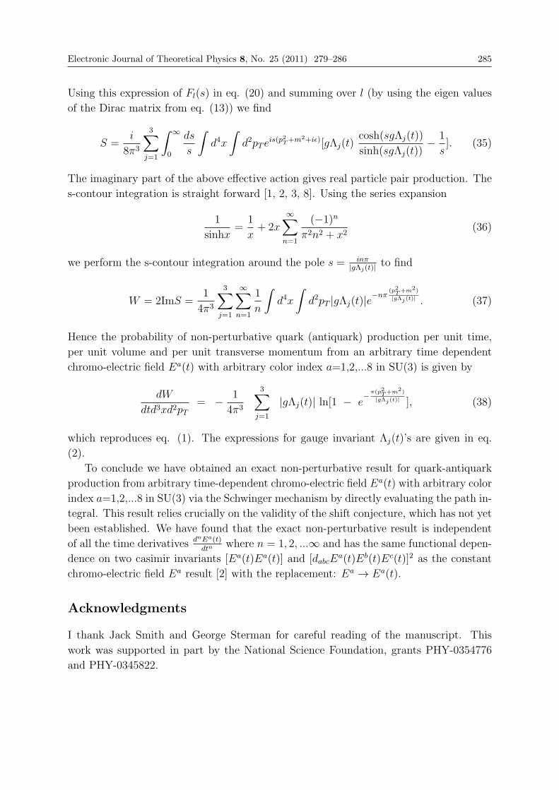
Electronic Journal of Theoretical Physics 8, No. 25 (2011) 279–286 285
Using this expression of Fl(s) in eq. (20) and summing over l (by using the eigen values
of the Dirac matrix from eq. (13)) we find
S =i
8π3
3∑j=1
∫ ∞
0
ds
s
∫d4x
∫d2pT e
is(p2T+m2+iε)[gΛj(t)cosh(sgΛj(t))
sinh(sgΛj(t))− 1
s]. (35)
The imaginary part of the above effective action gives real particle pair production. The
s-contour integration is straight forward [1, 2, 3, 8]. Using the series expansion
1
sinhx=1
x+ 2x
∞∑n=1
(−1)nπ2n2 + x2
(36)
we perform the s-contour integration around the pole s = inπ|gΛj(t)| to find
W = 2ImS =1
4π3
3∑j=1
∞∑n=1
1
n
∫d4x
∫d2pT |gΛj(t)|e
−nπ (p2T+m2)
|gΛj(t)| . (37)
Hence the probability of non-perturbative quark (antiquark) production per unit time,
per unit volume and per unit transverse momentum from an arbitrary time dependent
chromo-electric field Ea(t) with arbitrary color index a=1,2,...8 in SU(3) is given by
dW
dtd3xd2pT= − 1
4π3
3∑j=1
|gΛj(t)| ln[1 − e−π(p2T+m2)
|gΛj(t)| ], (38)
which reproduces eq. (1). The expressions for gauge invariant Λj(t)’s are given in eq.
(2).
To conclude we have obtained an exact non-perturbative result for quark-antiquark
production from arbitrary time-dependent chromo-electric field Ea(t) with arbitrary color
index a=1,2,...8 in SU(3) via the Schwinger mechanism by directly evaluating the path in-
tegral. This result relies crucially on the validity of the shift conjecture, which has not yet
been established. We have found that the exact non-perturbative result is independent
of all the time derivatives dnEa(t)dtn
where n = 1, 2, ...∞ and has the same functional depen-
dence on two casimir invariants [Ea(t)Ea(t)] and [dabcEa(t)Eb(t)Ec(t)]2 as the constant
chromo-electric field Ea result [2] with the replacement: Ea → Ea(t).
Acknowledgments
I thank Jack Smith and George Sterman for careful reading of the manuscript. This
work was supported in part by the National Science Foundation, grants PHY-0354776
and PHY-0345822.
286 Electronic Journal of Theoretical Physics 8, No. 25 (2011) 279–286
References
[1] J. Schwinger, Phys. Rev. 82 (1951) 664.
[2] G. C. Nayak, Phys. Rev. D72 (2005) 125010.
[3] G. Nayak and P. van Nieuwenhuizen Phys. Rev. D71 (2005) 125001; F. Cooper andG. C. Nayak, Phys. Rev. D73 (2006) 065005.
[4] G. C. Nayak, Eur. Phys. J. C59 (2009) 715.
[5] G. C. Nayak, Int.J.Mod.Phys.A25:1155-1163,2010.
[6] G. C. Nayak, JHEP 0903:051,2009.
[7] G. C. Nayak and F. Cooper, hep-th/0609192.
[8] C. Itzykson and J-B. Zuber, Quantum Field Theory, page-194, Dover Publication,Inc. Mineola, New York (1980).

EJTP 8, No. 25 (2011) 287–298 Electronic Journal of Theoretical Physics
Relic Universe
M.Kozlowski∗1 and J. Marciak-Kozlowska2
1Physics Department Warsaw University , Warsaw, Poland2Institute of Electron Technology , Warsaw, Poland
Received 6 July 2010, Accepted 10 February 2011, Published 25 May 2011
Abstract: In this paper we present the anthropic model calculation of the contemporary
Universe. The values of the radius Universe, velocity of expansion and acceleration are
calculated. In addition the cosmological parameter Λ in de Sitter Universe is calculated. We
argue that the present Epoch Universe is the Relic Universe. The future of the Universe is
diagnosed and discussed.c© Electronic Journal of Theoretical Physics. All rights reserved.
Keywords: Cosmology; Relic Universe; Anthropic Model; De Sitter Universe
PACS (2010): 98.80.-k; 98.80.Es; 04.60.-m
1. Introduction
In the recent years the growing interest for the source of Universe expansion is observed.
After the work of Supernova detecting groups the consensus for the acceleration of the
moving of the space time is established [2, 3]. In this paper we will developed the diffusion
model for the expansion of the Universe
We will study the influence of the repulsive gravity (G < 0) on the temperature
field in the universe and cosmological constant Λ. To that aim we will apply the quantum
hyperbolic heat transfer equation (QHT) formulated in our earlier papers [4, 5].
When substitution G→ −G is performed in QHT the Schrodinger type equation is
obtained for the temperature field. In papers [4, 5] the quantum heat transport equation
( diffusion equation) in a Planck Era was formulated:
τ∂2T
∂t2+∂T
∂t=
�
Mp
∇2T. (1)
In equation (1) τ =(�Gc5
)1/2is the relaxation time, Mp =
(�Gc
)1/2is the mass of the
∗ Corresponding author: e-mail: [email protected]

288 Electronic Journal of Theoretical Physics 8, No. 25 (2011) 287–298
Planck particle, h, c are the Planck constant and light velocity respectively and G is the
gravitational constant. The crucial role played by gravity (represented by G in formula
(28)) in a Planck Era was investigated in paper [5]. For a long time the question whether,
or not the fundamental constant of nature G varies with time has been a question of
considerable interest. Since P. A. M. Dirac [6] suggested that the gravitational force may
be weakening with the expansion of the Universe, a variable G is expected in theories such
as the Brans-Dicke scalar-tensor theory and its extension [7, 8]. Recently the problem of
the varying G received renewed attention in the context of extended inflation cosmology
[9]. It is now known, that the spin of a field (electromagnetic, gravity) is related to
the nature of the force: fields with odd-integer spins can produce both attractive and
repulsive forces; those with even-integer spins such as scalar and tensor fields produce
a purely attractive force. Maxwell’s electrodynamics, for instance can be described as a
spin one field. The force from this field is attractive between oppositely charged particles
and repulsive between similarly charged particles.
The integer spin particles in gravity theory are like the graviton, mediators of forces
and would generate the new effects. Both the graviscalar and the graviphoton are ex-
pected to have the rest mass and so their range will be finite rather than infinite. More-
over, the graviscalar will produce only attraction, whereas the graviphoton effect will
depend on whether the interacting particles are alike or different. Between matter and
matter (or antimatter and antimatter) the graviphoton will produce repulsion. The ex-
istence of repulsive gravity forces can to some extent explains the early expansion of the
Universe [6].
2. The Model
In this paper we will describe the influence of the repulsion gravity on the quantum
thermal processes in the universe. To that aim we put in equation (28) G → −G.In that case the new equation is obtained, viz.
i�∂T
∂t=
(�3 |G|c5
)1/2∂2T
∂t2−(�3 |G|c
)1/2
∇2T. (2)
For the investigation of the structure of equation (2) we put:
�2
2m=
(�3 |G|c
)1/2
(3)
and obtains
m =1
2Mp
with new form of the equation (2)
i�∂T
∂t=
(�3 |G|c5
)1/2∂2T
∂t2− �2
2m∇2T. (4)

Electronic Journal of Theoretical Physics 8, No. 25 (2011) 287–298 289
Equation (3) is the quantum Heaviside equation discussed in paper [5]. To clarify the
physical nature of the solution of equation (3) we will discuss the diffusion approximation,
i.e. we omit the second time derivative in equation (3) and obtain
i�∂T
∂t= − �2
2m∇2T. (5)
Equation (5) is the Schrodinger type equation for the temperature field in a universes
with G < 0.
Both equation (5) and diffusion equation:
∂T
∂t=
�2
2m∇2T (6)
are parabolic and require the same boundary and initial conditions in order to be “well
posed”.
The diffusion equation (5) has the propagator [10]:
TD
(R,Θ
)=
1
(4πDΘ)3/2exp
[− R2
2π�Θ
], (7)
whereR = r − r′, Θ = t− t′.
For equation (5) the propagator is:
TS
(R,Θ
)=
(Mp
2π�Θ
)3/2
exp
[−3πi
4
]exp
[iMpR
2
2π�Θ
](8)
with initial condition TS(R, 0) = δ(R)
3. The Anthropic Argument
In equation (8) TS((R), Θ) is the complex function of R and Θ. For anthropic observers
only the real part of T is detectable, so in our description of universe we put:
ImT(R,Θ
)= 0. (9)
The condition (9) can be written as (bearing in mind formula (8):
sin
[−3π4+
(R
Lp
)21
4Θ
]= 0, (10)
where LP=τP c and Θ = Θ/τp. Formula (10) describes the discretization of R
RN = [(4Nπ + 3π)Lp]1/2 (tc)1/2 ,
N = 0, 1, 2, 3...(11)

290 Electronic Journal of Theoretical Physics 8, No. 25 (2011) 287–298
In fact from formula (38) the Hubble law can be derived
RN
RN
= H =1
2τ, (12)
independent of N .
In the subsequent we will consider R (11), as the space-time radius of the N −universe with “atomic unit” of space LP .
It is well known that idea of discrete structure of time can be applied to the “flow”
of time. The idea that time has “atomic” structure or is not infinitely divisible, has
only recently come to the fore as a daring and sophisticated hypothetical concomitant
of recent investigations in the physics elementary particles and astrophysics. Descartes
[11]. The shortest unit of time, atom of time is named chronon [12]. Modern speculations
concerning the chronon have often be related to the idea of the smallest natural length
is LP . If this is divided by velocity of light it gives the Planck time τP=10−43 s, i.e. the
chronon is equal τP . In that case the time t can be defined as
t = M τ p, M= 0, 1, 2, . . . (12)
Considering formulae (10) and (12) the space-time radius can be written as
R(M,N) = π1/2M1/2
(N +
3
4
)1/2
Lp, M,N = 0, 1, 2, 3, .... (13)
Formula (13) describes the discrete structure of space-time. As the R(M , N) is time
dependent, we can calculate the velocity, υ = dR/dt, i.e. the velocity of the expansion of
space-time
υ =(π4
)1/2(N + 3
4
M
)1/2
c, (14)
where c is the light velocity. We define the acceleration of the expansion of the space-time
a =dυ
dt= −1
2
(π4
)1/2(N + 3
4
M3
)1/2c
τp. (15)
Considering formula (15) it is quite natural to define Planck acceleration:
Ap =c
τp=
(c7
�G
)1/2
= 1051ms−2 (16)
and formula (43) can be written as
a = −12
(π4
)1/2(N + 3
4
M3
)1/2(c7
�G
)1/2
. (17)
In Table I the numerical values for R, υ and a are presented. It is quite interesting
that for N , M →∞ the expansion velocity υ < c in complete accord with relativistic
description. Moreover for N , M >> 1 the υ is relatively constant υ =0.88 c. From

Electronic Journal of Theoretical Physics 8, No. 25 (2011) 287–298 291
formulae (38) and (42) the Hubble parameter H, and the age of our Universe can be
calculated
υ = HR,H = 12Mτp
= 5 · 10−18s−1,
T = 2Mτp = 2 · 1017s ∼ 1010years,(18)
which is in quite good agreement with recent measurement [13, 14, 15].
As is well known in de Sitter universe the cosmological constant Λ is the function of
R, radius of the Universe,
Λ =3
R2. (19)
Substituting formula (38) to formula (47) we obtain
Λ =3
πN2L2p
, N = 0, 1, 2.... (20)
The result of the calculation of the radius of the Universe, R, the acceleration of the
spacetime, a, and the cosmological constant, Λ are presented in Figs. 1, 2, 3, 4 for
different values of number N . As can be easily seen the values of a and R are in very
good agreement with observational data for present Epoch. As far as it is concerned
cosmological constant Λ for the firs time we obtain, the history of cosmological constant
from the Beginning to the present Epoch.
Conclusions
In this paper the diffusion model of the Universe expansion is developed. Considering the
anthropic argument Universe temperature :ImT( r,t) = 0 the quantization of the space-
time is obtained. The radius, velocity of the Universe expansion, the acceleration and
cosmological parameter as the function of the discreteness parameter N is obtained. For
N=10 60 the age Universe= 1017 s = the present Epoch. The present day Universe is
the relic of the primordial point Universe which expands in discrete steps N=1,2 ,. . . .
1060. . . .
References
[1] Kozlowski M.; Marciak – Kozlowska J. Thermal Processes Using Attosecond LaserPulses ; Optical Science 121; Springer: New York, NY, 2006.
[2] Adam G. Riess, Alexei V. Filippenko, Peter Challis, Alejandro Clocchiatti, AlanDiercks, Peter M. Garnavich, Ron L. Gilliland, Craig J. Hogan, Saurabh Jha, RobertP. Kirshner, B. Leibundgut, M. M. Phillips, David Reiss, Brian P. Schmidt, Robert A.Schommer, R. Chris Smith, J. Spyromilio, Christopher Stubbs, Nicholas B. Suntzeff,and John Tonry. Astron. J. 1998, 116, 1009.
[3] Glenn Starkman, Mark Trodden, and Tanmay Vachaspati. Phys. Rev. Lett. 1999, 83,1510.
[4] Marciak-Kozowska, J. Kozlowski M Found. Phys. Lett. 1997, 10, 295.

292 Electronic Journal of Theoretical Physics 8, No. 25 (2011) 287–298
[5] Kozlowski, M. ; Marciak – Kozlowska, J. Found. Phys. Lett. 1997, 10, 599.
[6] Dirac, P. A. M. Nature (London) 1937, 139, 323.
[7] Damour, T.; Gibbons, G. W.; Gundach, C. Phys. Rev. Lett. 1990, 64, 123.
[8] Damour, T.; Esposito Farese G. Esposito, Classical Quantum Gravity 1992, 9, 2093.
[9] La, D.; Steinhard, P. J. Phys. Rev. Lett. 1989, 62, 376.
[10] Barton, G. In Elements of Green’s functions and propagation, Oxford SciencePublications; Clarendon Press: Oxford, 1995; p. 222.
[11] Descartes, R. Meditions on the first philosophy. In A discourse on method etc.; Deut:London, 1912; pp 107-108.
[12] Whitrow, G. J. In The natural philosophy of time, 2nd Ed.; Oxford SciencePublications; Oxford, 1990; p. 204.
[13] R. Cayrel, V. Hill, T. C. Beers, B. Barbuy, M. Spite, F. Spite, B. Plez, J. Andersen,P. Bonifacio, P. Francois, P. Molaro, B. Nordstrom and F. Primas Nature, 2001, 409,691.
[14] Spergel D N, Bolte M. W Freedman, PNAS, 1997, 94, 6579.
[15] John D. Anderson, Philip A. Laing, Eunice L. Lau, Anthony S. Liu, Michael MartinNieto, and Slava G. Turyshev Phys. Rev. Lett., 1998, 81, 2858.
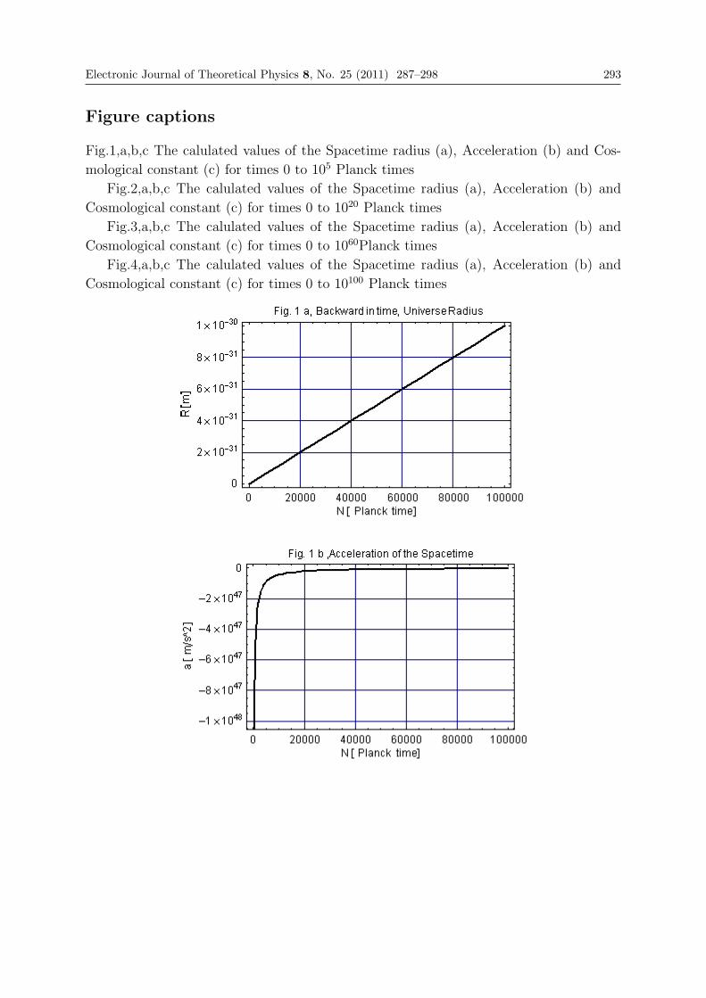
Electronic Journal of Theoretical Physics 8, No. 25 (2011) 287–298 293
Figure captions
Fig.1,a,b,c The calulated values of the Spacetime radius (a), Acceleration (b) and Cos-
mological constant (c) for times 0 to 105 Planck times
Fig.2,a,b,c The calulated values of the Spacetime radius (a), Acceleration (b) and
Cosmological constant (c) for times 0 to 1020 Planck times
Fig.3,a,b,c The calulated values of the Spacetime radius (a), Acceleration (b) and
Cosmological constant (c) for times 0 to 1060Planck times
Fig.4,a,b,c The calulated values of the Spacetime radius (a), Acceleration (b) and
Cosmological constant (c) for times 0 to 10100 Planck times

294 Electronic Journal of Theoretical Physics 8, No. 25 (2011) 287–298

Electronic Journal of Theoretical Physics 8, No. 25 (2011) 287–298 295

296 Electronic Journal of Theoretical Physics 8, No. 25 (2011) 287–298

Electronic Journal of Theoretical Physics 8, No. 25 (2011) 287–298 297


EJTP 8, No. 25 (2011) 299–310 Electronic Journal of Theoretical Physics
Halo Spacetime
Mark D. Roberts∗†
54 Grantley Avenue, Wonersh Park, GU5 0QN, UK
Received 12 March 2011, Accepted 5 April 2011, Published 25 May 2011
Abstract: It is shown that constant galactic rotation curves require a logarithmic potential
in both Newtonian and relativistic theory. In Newtonian theory the density vanishes
asymptotically, but there are a variety of possibilities for perfect fluid Einstein theory.c© Electronic Journal of Theoretical Physics. All rights reserved.
Keywords: Cosmology; Galactic Rotation; Halo Spacetime; Logarithmic Newtonian Potential;
Einstein Equations
PACS (2010): 98.80.-k; 04.20.Fy; 04.20.-q; 98.62.En; 04.40.Nr
1. Introduction.
Constant galactic rotation curves require a logarithmic potential in both newtonian and
relativistic theory. The logarithmic potential contrasts with heuristic derivations of the
Tully-Fischer [4, 7] relationship, which require φ ≈ 1/r. As pointed out in [18] for
a potential ≈ ln(r) one would expect as well a metric with ≈ ln(r) terms and hence
first derivatives and Christoffel symbol corresponding to the metric are of order ≈ 1/r;
thus both the derivatives and products of the Christoffel symbol are of order ≈ 1/r2 so
that linear approximations to the Riemann tensor and hence the field equations are not
necessarily consistent. This is why for a relativistic analysis one has to start again with
the properties of geodesics, this is done here in section 3.. A problem with any model
of galactic rotation is what happens asymptotically. The logarithmic potential necessary
for constant rotation curves diverges as r → ∞. One way around a divergent potential
seems to be to invoke a “halo” which is a region surrounding a galaxy where there is an
approximately logarithmic newtonian potential. The properties of the “halo” have some
sort of unspecified cut off so that the potential does go out to too large distances, quite
how this works is not at all clear, after all binary and multiple galaxies exhibit unusual
∗ [email protected]† http://www.violinist.com/directory/bio.cfm?member=robemark

300 Electronic Journal of Theoretical Physics 8, No. 25 (2011) 299–310
dynamics, as do stellar clusters, but presumably nearby galaxies have more gravitational
influence than distant ones, so that at some distance a logarithmic potential must have
a cut off. Another way of looking at what happens asymptotically for a logarithmic
potential is to note that it is only the derivatives of the potential that have effects and
φr ≈ 1/r does not diverge asymptotically. Yet another way is to introduce smooth step
functions, see section 5.. “Halo” is a term that is usually restricted to an area of “dark
matter” surrounding a galaxy; however if a model uses matter fields or different field
equations to model galactic rotation one would again require a region that these fields
model and it is simpler to again refer to this as a “halo” rather than use new terminology.
In section 4. the analysis is generalized to the perfect fluid Einstein equations where
it is shown that the density is the same as in the Newtonian analysis, but with addi-
tional terms appearing in the pressure and the density of order v4c . The analysis requires
four assumptions: 1)a galactic halo can be modelled by a static spherically symmetric
spacetime, 2)in the limit of no rotation halo spacetime is Minkowski spacetime, 3)the con-
straint on the first derivatives of the metric needed in order to produce constant rotation
curves can be applied, 4)the perfect fluid Einstein equations; the density is the same as
in the Newtonian analysis, but with additional terms appearing in the pressure and the
density of order v4c . The assumption 1) is that a galactic halo can be modelled by a static
spherically symmetric spacetime. That it is static is a good approximation as dynamical
disturbances in galaxies do not seem to be the cause of constant rotation curves. That it
is spherically symmetric seems to be born out by observations [14]. Thus it is taken that
a spherically symmetric halo causes constant galactic rotation, rather than the rotation of
the luminous part of the galaxy. Using spherical symmetry as opposed to axial symmetry
considerably simplifies calculations. There are two problems with the assumption 2) that
in the limit of no rotation the spacetime is Minkowski spacetime. The first is that it ex-
cludes the possibility of other limiting structure, such as deSitter spacetime. The second
is that even non-rotating galaxies have non-flat spacetimes: in other words this assump-
tion is that to lowest order the rotating part of the description of a galaxies spacetime can
be described independently of its non-rotating part. The assumption 3) is the constant
velocity rotation constraint, this is a constraint on the first derivatives of the metric, it
has been derived in [19], and is derived again in the next section. For spherical symme-
try it is an unusual constraint because it often involves logarithms rather than powers
of the metric. The assumption 4) is the perfect fluid Einstein equations. For spherical
symmetry the stress has three arbitrary stress functions (ρ, pr, pθ). The assumption that
the stress is a perfect fluid reduces the three components to two (ρ, p) via the isotropic
pressure equation p = pr = pθ. For a perfect fluid the density ρ and the pressure p are
independent unless an equation of state is imposed. The reduction of the three arbitrary
stress functions to two can be thought of as a second constraint on a first derivative of
the metric. The fourth assumption has two aspects: firstly that Einstein’s equations are
the correct ones to model galaxies, and secondly that any ”dark matter” has isotropic
pressure so that pr = pθ. In section 4. whether it is permissible to expand in the velocity
of rotation vc/c, where c is the velocity of light, rather than a radial parameter r is also

Electronic Journal of Theoretical Physics 8, No. 25 (2011) 299–310 301
discussed. For a galaxy it is not clear what radial parameter could be used because of
the problem of what happens as r → ∞, for the luminosity radial parameter R one has
that the metric ≈ ln(R) suggesting that it is not a good parameter to expand in. In both
cases the expansions are independent of the mass of the galaxy m which does not enter
explicitly into calculations here to lowest order. Taking galactic rotation to be in any
way related to the Kerr solution is always misleading, as Kerr rotation is a short range
effect and galactic rotation is a long range effect.
A selection of recent literature on rotation curves can be divided into three types.
The first are papers which use the MOND modification of gravity, see for example [2, 3].
The second are papers which invoke higher dimensions and/or branes, see for example
[8, 10, 11, 13, 15]. The third are papers which invoke new fields, or field equations, or
potentials, see for example [1,5,6,12,16-18,22-24].
Conventions include: metric -+++ and field equations Gab = 8πGTab Calculations
were done using maple9.
2. Newtonian theory.
First a newtonian analysis is given, the presentation follows [19], but is shorter. In
spherical coordinates newton’s second law has two dynamical components
− (φr, φθ) =
(r − rθ2,
d
dr(r2θ)
), (1)
where φ is the newtonian potential and the subscript indicates which coordinate it is
differentiated with. The θ component integrates to give
r2θ = L, (2)
where L is the angular momentum for each individual particle. The square of the velocity
at any point is
v2 = r2 + (rθ)2. (3)
For circular orbits r = 0 so that (3) becomes
v2c = (rθ)2 =L2
r2, (4)
also for circular orbits Newton’s second law (1) gives
φr = rθ2 =L2
r3. (5)
Eliminating L2 from these two equations (4) and (5) gives
φr =v2cr, (6)
integrating gives the newtonian potential
φ = v2c ln(r), (7)

302 Electronic Journal of Theoretical Physics 8, No. 25 (2011) 299–310
where vc is a constant. Poisson’s equation is
4πGρ = �φ =1
r2(r2φr
)r=v2cr2. (8)
3. The Geodesics of Rotation Curves
The constant rotation curve constraint can be derived as follows. The axi-symmetric line
element can be taken as
ds2 = gttdt2 + 2gtφdtdφ+ gφφdφ
2 + grrdr2 + gθθdθ
2. (9)
The geodesic lagrangian is
2L = gttt2 + 2gtφtφ+ gφφφ
2 + grrr2 + gθθθ
2 = papa, (10)
where 2L = −1 for timelike geodesics. The Euler equations are
dpadτ
=∂L∂xa
. (11)
For (10)
pr ≡∂L∂r
= grrr, 2∂L∂r
= g′ttt2 + 2g′tφtφ+ g′φφφ
2 + g′rrr2 + g′θθθ
2, (12)
where f ′ denotes ∂f/∂r. Thus the r component of the Euler equation is
dprdτ
= grrr + g′rrr2 + grr,θrθ = g′ttt
2 + 2g′tφtφ+ g′φφφ2 + g′rrr
2 + g′θθθ2, (13)
with a similar equation for the θ component. If required the pt and pφ components can
be expressed in terms of the energy E and momentum L for each geodesic, and then with
(13) this allows generalizations of the Binet equation; however for present purposes this
is unnecessary as the problem much simplifies because constant velocity curves require
θ = r = 0. (14)
Substituting into the lagrangain (10) and the r & θ components of the Euler equation
(13) gives
2L = gttt2 + 2gtφtφ+ gφφφ
2, (15)
0 = g′ttt2 + 2g′tφtφ+ g′φφφ
2,
respectively. There is a similar equation to the second of (15) with f ′ denoting ∂f/∂θ.The angular momentum is
Ω ≡ φ
t=
vc√gφφ
, (16)
note that this corrects equation (27) of [19] where there is an r rather than a√gφφ in
the denominator of the last term. Substituting into the lagrangian equation of (15) from

Electronic Journal of Theoretical Physics 8, No. 25 (2011) 299–310 303
which t can be calculated, this is not necessary for present purposes. Substituting into
(15) first for the first equality in (16) and then for the second equality in (16) gives
0 = g′tt + 2g′tφΩ + g′φφΩ2 = g′tt + 2
vc√gφφ
gtφ +v2cg
′φφ
gφφ. (17)
There is the possibility the galactic rotation curves are intrinsically axi-symmetric and
cannot be modelled by spherical symmetry, however the newtonian model with potential
7 is spherically symmetric and if there is a requirement that this is a limit of a relativis-
tic model then to lowest order this must also be spherically symmetric. For spherical
symmetry with line element
ds2 = − exp(2ν)dt2 + exp(2μ)dr2 + exp(2ψ)dΣ22, (18)
where dΣ22 = dθ2 + sin(θ)2dφ2, the constraint (17) reduces to
{exp(2ν)}′ = 2v2cψ′. (19)
The requirement that for vc = 0 the metric is Minkowski fixes the constant of integration;
integrating the metric becomes
ds2 = −(1 + 2v2cψ(r)
)dt2 + exp(2μ(r))dr2 + exp(2ψ(r))dΣ2
2. (20)
At first sight this line element has two arbitrary function in it, however defining the
luminosity distance rlm
rlm ≡ exp(ψ(r)), exp(μlm(rlm) ≡exp(μ(invψ(ln(rlm))))
r2lmψ2r
, (21)
and dropping the subscript lm the line element becomes
ds2 = −(1 + 2v2c ln(r))dt2 + exp(2μ)dr2 + r2dΣ2
2, (22)
leaving just one arbitrary function μ(r). This can be fixed by using field equations.
4. The Perfect Fluid Einstein Equations
For a spherically symmetric spacetime of the form (22) there are three non-vanishing
components of the Einstein tensor
8πGρ = −Gt.t =
1
r2(1− (r exp(−2μ))′), (23)
8πGpr = +Gr.r =
1
r2
(−1 + exp(−2μ)(1 + 2v2c + 2v2c ln(r))
(1 + 2v2c ln(r))
)8πGpθ = +Gθ
.θ =− exp(−2μ)
r2(1 + 2v2c ln(r))
(v4c
(1 + 2v2c ln(r))+ rμ′(1 + v2c + 2v2c ln(r))
)where Gφ
.φ = Gθ.θ, ρ is the density, pr is the radial pressure, and pθ is the angular pres-
sure. These field equations are simple as they linear in only the first derivatives of μ

304 Electronic Journal of Theoretical Physics 8, No. 25 (2011) 299–310
and so should have many solution, for present purposes just the case of a perfect fluid
is examined. The requirement that the stress be that of a perfect fluid is that the pres-
sure is isotropic p = pr = pθ, and this is sufficient to completely determine the metric.
Subtracting pθ from pr gives a first order differential equation in μ,
rμ′ +1 + v2c + 2v2c ln(r)
1 + 2v2c ln(r)+ exp(2μ)
(r2(pθ − pr)− 1
) 1 + 2v2c ln(r)
1 + v2c + 2v2c ln(r)= 0, (24)
setting pθ = pr and solving gives
ds2 = −(1− 2v2c ln(r))dt2 +
dr2
2r2(k − I)(1 + 2v2c ln(r))+ r2dΣ2
2, (25)
the requirement that the line element reduces to Minkowski when the velocity vanishes
gives k = 0. I is the integral
I ≡∫dr
r31
(v2c + 1 + 2v2c ln(r))(26)
= − 1
2r2+ (1 + ln(r))
v2cr2−(5 + 8 ln(r) + 4 ln(r)2
) v4c2r2
+O(v6c).
For k = 0 the pressure is
8πGp = − 1
r2+ 2
(1 + 2v2c + 2v2c ln(r)
)(k − I) =
v4cr2+O
(v6c), (27)
and the density is
8πGρ =(3 + v2c + 6v2c ln(r))
(1 + v2c + 2v2c ln(r))r2+ 2
(3 + 2v2c + 6v2c ln(r)
)(I − k) (28)
= +2v2cr2− (9 + 4 ln(r))
v4cr2+O
(v6c).
The O(v0c ) term of the integral (27) shows that the spacetime is Minkowski when vc =
k = 0, for k �= 0 the grr component looks similar to deSitter spacetime however there is
no corresponding term in gtt and any such term would violate the the rotation constraint
(17), here usually k = 0. The expansion in vc shows that to lowest order the density
(28) agrees with the newtonian expression (8), however the expansion does not always
converge, terms becoming larger and changing sign for each increase in v2c . The large
distance r properties of (28) cannot be obtained from the v2c expansion as this is not
the same as a r−2 expansion because of the ln(r) terms. The technical reason that a
r−2 expansion cannot be obtained is that there is no series expansion for the logarithmicintegral J ≡
∫dx/ ln(x), if it is attempted each term is of the same order. This makes it
necessary to work with the exponential integral defined by
Ei(a, z) ≡∫ ∞
1
d�
�aexp (−�z) , (29)
and illustrated in the figure.

Electronic Journal of Theoretical Physics 8, No. 25 (2011) 299–310 305
Fig. 1 The logarithmic and exponential integrals.
Fig. 2 The density, pressure and mass function.
Using this definition 29 the integral 27 can be expressed as
I = − 1
2v2cexp
(1 +
1
v2c
)Ei
(1, 1 +
1
v2c+ 2 ln(r)
), (30)
and this can be used to numerically produce graphs of the properties of the spacetime. In
figure one the density, 105×pressure and 400×mass function are plotted for vc/c = 0.05
(not v2c = 0.05) and k = 0. Asymptotically the density approaches 3, the pressure 0,
and the mass function r. In the region vc = 0.01 − 0.02 the machine overflows, which
is unfortunate as vc = 10−6 is a more realistic value. For k = 1 the density and mass
function appear negative, the critical value for which positive density is restored is around
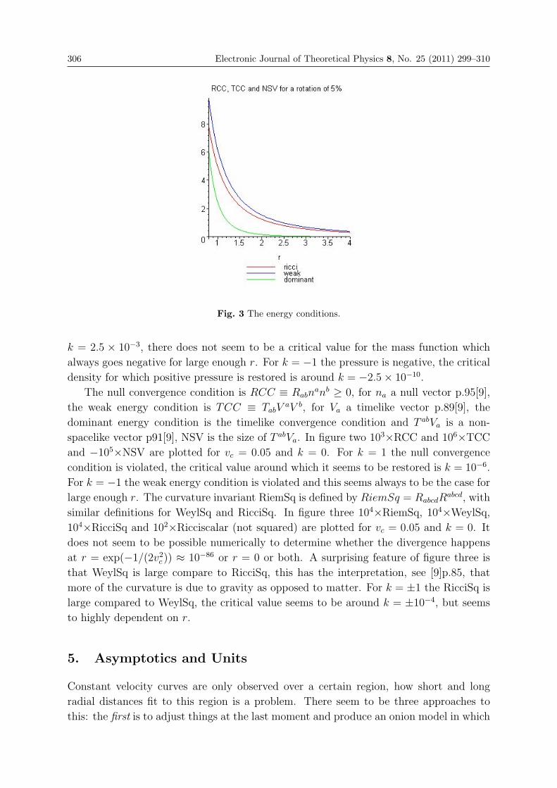
306 Electronic Journal of Theoretical Physics 8, No. 25 (2011) 299–310
Fig. 3 The energy conditions.
k = 2.5 × 10⁻³, there does not seem to be a critical value for the mass function which
always goes negative for large enough r. For k = −1 the pressure is negative, the criticaldensity for which positive pressure is restored is around k = −2.5× 10⁻¹⁰.
The null convergence condition is RCC ≡ Rabnanb ≥ 0, for na a null vector p.95[9],
the weak energy condition is TCC ≡ TabVaV b, for Va a timelike vector p.89[9], the
dominant energy condition is the timelike convergence condition and T abVa is a non-
spacelike vector p91[9], NSV is the size of T abVa. In figure two 103×RCC and 106×TCC
and −105×NSV are plotted for vc = 0.05 and k = 0. For k = 1 the null convergence
condition is violated, the critical value around which it seems to be restored is k = 10−6.For k = −1 the weak energy condition is violated and this seems always to be the case forlarge enough r. The curvature invariant RiemSq is defined by RiemSq = RabcdR
abcd, with
similar definitions for WeylSq and RicciSq. In figure three 104×RiemSq, 104×WeylSq,
104×RicciSq and 102×Ricciscalar (not squared) are plotted for vc = 0.05 and k = 0. It
does not seem to be possible numerically to determine whether the divergence happens
at r = exp(−1/(2v2c )) ≈ 10−86 or r = 0 or both. A surprising feature of figure three is
that WeylSq is large compare to RicciSq, this has the interpretation, see [9]p.85, that
more of the curvature is due to gravity as opposed to matter. For k = ±1 the RicciSq islarge compared to WeylSq, the critical value seems to be around k = ±10−4, but seemsto highly dependent on r.
5. Asymptotics and Units
Constant velocity curves are only observed over a certain region, how short and long
radial distances fit to this region is a problem. There seem to be three approaches to
this: the first is to adjust things at the last moment and produce an onion model in which

Electronic Journal of Theoretical Physics 8, No. 25 (2011) 299–310 307
Fig. 4 The curvature invariants.
Fig. 5 A good newtonian potential.
the constant velocity region as given has other spacetimes are fixed to it, see [20], the
second is to adjust things in the middle by choosing contrived newtonian potentials, the
third is to adjust things at the beginning by letting vc → vc(r).
Looking at the third approach first, for a newtonian model, equations (6) and (8)
become
rφr = v2c (r), 4πGρ =1
r2(rv2c (r)
)′. (31)
For purposes of illustration consider the smoothed out step around r = ro
S(r, ro) ≡1
2(1− tanh(r − ro)) =
1
exp(2(r − r0)) + 1. (32)
Apply the step (32) to the velocity
v2c (r, ro) = S(r, ro), (33)

308 Electronic Journal of Theoretical Physics 8, No. 25 (2011) 299–310
then the potential is given by an integral, (34) with k = 1, The integral (34) has to be
evaluated numerically
φ =
∫dr
r(exp(2(r − ro) + k), (34)
for the velocity (33), (31) gives the density
4πGρ =1 + (1− 2r) exp(2(r − ro)
r2(1 + exp(2(r − ro)))2(35)
For ro = 4 the velocity (33), the potential (34) divided by 3.5 and the density (35) divided
by 100 are plotted in figure four, to avoid singularities at the origin the integral is taken
from 0.1 rather than 0. By comparison with the integral∫dr/(exp(2(r − ro) + 1) =
ln(exp(2(r− ro))/(exp(2(r− ro))+1))/2 the potential converges to 0 as r →∞, which is
good for two reasons, firstly that it converges at all unlike ln(r), secondly that the limit
is 0 so that there is no trace of the potential at great distance from the galaxy; similarly
comparing with the integral∫dr/r = ln(r) the potential is seen to diverge for short
distances. Surprisingly both the potential and the density show no unusual properties at
the step ro.
For the second approach apply the step (32) to the potential so that
φ = ln(r)S(r), v2c := r(ln(r)S(r))′ (36)
the potential starts out like a ln potential and then smooths out, however v2c becomes
negative which is unphysical.
For short distance behaviour one can again use smoothed out step functions, however
numerical studies show that there are rings of large density near the smoothed out step.
To produce a relativistic model with potential (34) is a substantial numerical problem: one
needs to first evaluate the integral numerically, then substitute this into the generalization
of (24) to solve that numerically, and finally put this into the generalizations of (23) to
get the pressure and density.
Another problem is what units of length r is measured in. As galactic rotation curves
are observed to be constant at almost all distances from the centre of galaxies, the problem
is in this sense scale invariant and there is no characteristic length scale for the problem.
The models here are invariant under r → r/r0 so that r is arbitrary, in particular the
models here of galactic rotation do have a characteristic length, usually when r = 1 where
ln(r) changes sign, so the question arises ‘what is r = 1 in meters?’, the answer is that this
is an arbitrary distance. An exception is the model (34) where there is no characteristic
length associated with a sign change of the potential, but there is the characteristic length
of the step at ro.
Conclusion.
That galactic rotation is described by a logarithmic potential, as opposed to a reciprocal
potential −1/r, is sufficient to show that dark matter does not exist. In particular Fig.2

Electronic Journal of Theoretical Physics 8, No. 25 (2011) 299–310 309
shows that both the density and mass function do not tend to zero asymptotically. Thus
galactic rotation requires field modifications as opposed to fluid modifications of Einstein’s
equations, such a field model has been given [21].
Acknowledgements.
I would like to thank Jakob Bekenstein, James Binney, Antony Fairall, Alex Feinstein,
Gerry Gilmore, Tom Kibble, Andrew Liddle, David Matravers, Michael Merrifield and
Andrew Taylor for discussion on various aspect of this paper, and the referee for his
comments.
References
[1] Alexandre Arbey, Julien Lesgourgues & Pierre SalatiCosmological constraints on quintessential halos.http://arxiv.org/abs/astro-ph/0112324 astro-ph/0112324
[2] J.D. BekensteinRelativsitic gravitational theory for the MOND paradigm.http://arXiv.org/abs/astro-ph/0403694 astro-ph/0403694
[3] K.G. Begeman, A.H. Broeils et alExtended rotation curves of spiral galaxies: dark haloes and modified dynamics.Mon.Not.R.Astr.Soc.249(1991)524-537.
[4] M. CarmeliDerivation of the Tully-Fisher Law: Doubts about the necessity and existence of halodark matter.Int.J.Theor.Phys.39(2000)1397-1404.
[5] F.I. Cooperstock & S. TieuGeneral relativity resolves galactic rotation without exotic dark matter.http://arxiv.org/abs/astro-ph/0507619 astro-ph/0507619
[6] Donald H. EchardtExponential potential versus dark matter.Phys.Rev.D48(1993)3762-3767.
[7] John G. HartnettCan the Carmeli metric correctly describe galaxy rotation curves?http://arxiv.org/abs/astro-ph/0407082 astro-ph/0407082
[8] Tiberiu Harko & K.S. ChengGalactic metric, dark radiation, dark pressure and gravitational lensing in braneworld models.http://arxiv.org/abs/astro-ph/0509576 astro-ph/0509576
[9] Hawking, S. W. and Ellis, G. F. R. (1973)The Large Scale Structure of Space-time.Math.Rev.http://www.ams.org/mathscinet-getitem?mr=54:12154 54 #12154,Cambridge University Press.
[10] Dan Hooper & Graham D. KribsKaluza-Klein dark matter and the positron excess.http://arxiv.org/abs/hep-ph/0406026 hep-ph/0406026

310 Electronic Journal of Theoretical Physics 8, No. 25 (2011) 299–310
[11] Kimmo Kainulainen & Daniel Sunhede, DanielDark Energy from Large Extra Dimensions.http://arxiv.org/abs/hep-ph/0412609 hep-ph/0412609
[12] V.V. KislevGhost condensate model of flat rotation curves.http://arxiv.org/abs/gr-gc/0406086 gr-qc/0406086
[13] M.K. Mak & Tiberiu HarkoCan the galatic rotation curves be explained in brane world models?Phys.Rev.D70(2004)024010.
[14] Michael R. MerrifieldHalo Tracing with Atomic Hydrogen.http://arxiv.org/abs/astro-ph/0107291 astro-ph/0107291
[15] Supralik Pal, Somnath Bharadwaj & Sayan KarCan extra dimensional effects replace dark matter?http://arxiv.org/abs/gr-qc/0409023 gr-qc/0409023
[16] Mark D. RobertsMach’s Principle and the Missing Mass in Clusters of Galaxies.Acta Phys.Polon.B16(1985)693-697.
[17] Mark D. RobertsA new approach to a relativistic model of galaxies.Astrophysics & Space Science119(1986)405-407.
[18] Mark D. RobertsGalactic Rotation Curves and Quadratic Lagrangians.Mon.Not.roy.Astro.Soc.249(1991)339-342.
[19] Mark D. RobertsGalactic Metrics.http://arXiv.org/abs/astro-ph/0209456 astro-ph/0209456Gen.Rel.Grav.36(2004)1-10.
[20] Mark D. RobertsSpacetime Exterior to a Star.http://arXiv.org/abs/gr-qc/9811093 gr-qc/9811093 International Journal ofTheoretical Physics(2004)1-37.
[21] Mark D. RobertsString theory explanation of galactic rotation.http://arXiv.org/abs/1003.1309 1003.1309
[22] Daniel Vogt & P.S.LetelierRelativistic Models of Galaxies.http://arxiv.org/abs/astro-ph/0507406 astro-ph/0507406
[23] Xavier Hernandez, Tonatiuh Matos, Roberto A. Sussman and Yosef VerbinScalar field ”mini-MACHOs”: a new explanation for galactic dark matter.http://arxiv.org/abs/astro-ph/0407245 astro-ph/0407245
[24] V.V. Zhytnikov & J.M. NesterCan Galactic Observations Be Explained by a Relativistic Gravity Theory?Phys.Rev.L73(1994)2950.

EJTP 8, No. 25 (2011) 311–318 Electronic Journal of Theoretical Physics
C-field Barotropic Fluid Cosmological Model withVariable G in FRW space-time
Raj Bali∗ and Meghna Kumawat†
Department of Mathematics, University of Rajasthan, Jaipur-302055, India
Received 6 July 2010, Accepted 10 February 2011, Published 25 May 2011
Abstract: C-field cosmological model with variable G for barotropic perfect fluid distribution
in flat FRW (Friedmann-Robertson-Walker) space-time is investigated. To get the deterministic
model of the universe, we assume that G = Rn where R is scale factor and n is a constant.
We find that the creation field (C) increases with time, G and ρ (matter density) decreases
with time and∣∣∣ GG
∣∣∣ = H(t) where H is the Hubble parameter. These results match with the
observations.c© Electronic Journal of Theoretical Physics. All rights reserved.
Keywords: C-field Cosmology; Variable G; FRW space-time
PACS (2010): 98.80.Cq; 04.20.-q
1. Introduction
In Einstein’s General Theory of Relativity, the gravitational constant (G) plays the role
of coupling constant between geometry and matter. Therefore, in an evolving universe,
it is natural to look at this constant which depends on time based on different arguments
proposed in last few decades. Motivated by the occurrence of large numbers hypoth-
esis, Dirac [1] proposed a theory with a variable gravitational constant. Subsequently,
mathematically well posed alternative theories of gravity were developed to generalize
Einstein’s general theory of relativity by including variable G and satisfying conservation
equation. The scalar tensor theory of gravity was first formulated by Jordan [2]. To
achieve possible unification of gravitation and elementary particle physics or to incorpo-
rate Mach’s principle in general relativity, many attempts (Brans and Dicke [3], Hoyle
and Narlikar [4,5], Canuto et al. [6]) have been proposed for the possible extensions of
∗ E-mail: [email protected]† E-mail: meghnaa [email protected]
312 Electronic Journal of Theoretical Physics 8, No. 25 (2011) 311–318
Einstein’s general relativity with time dependent G.
The astronomical observations reveal that the predictions of Friedmann-Robertson-
Walker (FRW) type models do not meet our requirements as was developed earlier (Smoot
et al. [7]). Thus alternative theories were proposed from time to time. The most well
known theory is the Steady State Theory by Bondi and Gold [8]. In this theory, the
universe does not have any singular beginning nor an end on the cosmic time scale. For
the maintenance of uniformity of mass density, they envisaged a very slow but contin-
uous creation of matter in contrast to the explosive creation at t = 0 of the standard
model. However, it suffers from the serious disqualifications by not giving any physical
justifications in the form of any dynamical theory for continuous creation of matter. To
overcome this difficulty, Hoyle and Narlikar [9] adopted a field theoretic approach intro-
ducing a massless and chargeless scalar field to account for creation of matter. In C-field
theory, there is no big-bang type singularity as in the steady-state theory of Bondi and
Gold [8]. Narlikar [10] has explained that matter creation is accomplished at the expense
of negative energy C-field. He also emphasized that if overall energy conservation is to be
maintained then primary matter creation must be accompanied by the release of nega-
tive energy and the repulsive nature of this negative reservoir will be sufficient to prevent
the singularity. Narlikar and Padmanabhan [11] investigated the solution of Einstein’s
field equation which admits radiation and negative energy massless scalar creation field
as a source. Vishwakarma and Narlikar [12] discussed modeling repulsive gravity with
creation. Recently Bali and Tikekar [13] have investigated C-field cosmological model for
dust distribution with variable G in the frame work of flat Friedmann-Robertson-Walker
space-time and the results match with the observations.
In this paper, we have investigated C-field barotropic perfect fluid cosmological model
with variable G using flat FRW space-time. In particular, we obtain the same result for
dust distribution for C-field cosmological model with variable G in flat FRW model as
obtained by Bali and Tikekar[13]. The physical aspects of the model have been discussed
and the results match with the observations.
2. Formation of Line-Element
We consider the flat FRW space-time as
ds2 = dt2 − R2(t)[dr2 + r2 dθ2 + r2sin2θdφ2] (1)
Einstein’s modified field equations by the introduction of C-field are given by (Narlikar
[15]) as
Rj
i −1
2Rg
j
i = − 8 π G(mT j
i +CT
j
i ) (2)
wheremT j
i = ( ρ+ p) vi vj − pgji (3)
andCT j
i = − f(CiC
j − 1
2gji C
αCα
)(4)

Electronic Journal of Theoretical Physics 8, No. 25 (2011) 311–318 313
with f > 0 and Ci =dCdxi .
The modified field equation (2) for the metric (1) for variable G(t) leads to
3R2
R2= 8 π G(t)
(ρ − 1
2fC
2)
(5)
2R
R+
R2
R2= 8 π G(t)
(1
2fC
2 − p
)(6)
The conservation equation
(8 π GT ji );j = 0
leads to
8 π G
(ρ− 1
2fC
2)+ 8 π G
(ρ− fC C − 3fC
2 R
R+ 3 (ρ+ p)
R
R
)= 0 (7)
which yields C = 1when used in the source equation.
Using C = 1 in equation (5), we have
8 π Gρ =3R
2
R2+ 4 π Gf (8)
We assume that universe is filled with barotropic perfect fluid i.e. p = γρ(0 ≤ γ ≤ 1),p
being the isotropic pressure, ρ the matter density. Now using p = γρ and C = 1 in
equation (6), we have2R
R+R2
R2= 4 π Gf − 8 πGγρ (9)
Equations (8) and (9) lead to
2R
R+ (1 + 3γ)
R2
R2= (1− γ)4πG(t)f (10)
To get the deterministic solution, we assume that
G = Rn (11)
where R is the scale factor and n is a constant.
Using the condition (11) in (10), we have
2R + (1 + 3γ)R2
R= (1− γ)KRn+1 (12)
where
K = 4 π f (13)
Let us assume R = F (R). Thus equation (12) leads to
d
dR(F 2) +
(1 + 3γ
R
)F 2 = (1− γ)KRn+1 (14)

314 Electronic Journal of Theoretical Physics 8, No. 25 (2011) 311–318
where
R = FF′, F
′=dF
dR.
From equation (14), we have
F 2 =
(dR
dt
)2
=K(1− γ)Rn+2
n+ 3γ + 3+
L
R3γ+1(15)
where L is the constant of integration. Equation (15) leads to
R3γ+1
2 dR√K(1− γ)Rn+3γ+3 + L(n+ 3γ + 3)
=dt√
n+ 3γ + 3(16)
where L is the constant of integration.
To obtain the deterministic value of R in terms of cosmic time t, we assume that
n = −(3γ + 3
2
)(17)
Using condition (17) in (16), we have
R3γ+1
2 dR√R
3γ+32 + L(3γ+3)
2K(1−γ)
=
√2K(1− γ)
3γ + 3dt (18)
Equation (18) leads to
R3γ+3
2 =
⎡⎣{1
2
√K(1− γ)(3γ + 3)
2t+
(3γ + 3
4
)N
}2
− L(3γ + 3
2K(1− γ)
⎤⎦ (19)
where N is the constant of integration. Therefore
G = Rn = R−3γ+3
2 =
⎡⎣{1
2
√K(1− γ)(3γ + 3)
2t+
(3γ + 3
4
)N
}2
− L(3γ + 3)
2K(1− γ)
⎤⎦−1(20)
From equations (8), (19) and (20), we have{3K(1− γ)(3γ + 3)
2+K
(3γ + 3
2
)2} {√
K(1− γ)(3γ + 3)
2√2
t+N(3γ + 3)
4
}2
− L
8
(3γ + 3)3
(1− γ)
8 πρ = (3γ+32
)2 [{√3K(1−γ2)
2√2
t+ 3(1+γ)N4
}− 3L(1+γ)
2K(1−γ)
] (21)
Using barotropic equation p = ργ in equation (7), we have

Electronic Journal of Theoretical Physics 8, No. 25 (2011) 311–318 315
8 π (Gρ+ Gρ)− 4πGfC2 −− 8 πGfCC
−24πGρRRfC
2+ 24πGρ
R
R(1 + γ) = 0 (22)
Equation (22) after using (19), (20) and (21) leads to
C2t6−2γ1+γ =
∫ [9(1−γ2)
2+ 9(1+γ)2
4
]9(1+γ)2
8
t5−3γ1+γ dt (23)
where we have set the constants of integration L = 0, N = 0 to get the deterministic
value of C. Now equation (23) leads to
C2.t6−2γ1+γ =
36(1− γ2) + 18(1 + γ)2
9(1 + γ)
t6−2γ1+γ
6− 2γ+M
= 4(1−γ)+ 2(1+γ)2(3−γ) t
6−2γ1+γ (setting M = 0)
=6− 2γ
6− 2γt6−2γ1+γ (24)
Thus, we have
C2 = 1 (25)
which leads to
C = t (26)
We find that C = 1 which agrees with the value used in source equation. The creation
field (C) increases with time. The metric (1) after using the value of R, leads to
ds2 = dt2 −{√
3K(1− γ2)
2√2
t
} 83γ+3
[dr2 + r2dθ2 + r2sin2θdφ2] (27)
where γ �= 1.
Special Cases
i) γ = 0 gives that FRW model for dust distribution with variable G obtained by Bali
and Tikekar [13].
ii) γ = 1/3 i.e. ρ = 3p gives radiation dominated universe for flat FRW model with
variable G.
iii) γ = 1 leads to stiff fluid universe but in our case flat FRW model with variable G is
not possible for γ = 1.

316 Electronic Journal of Theoretical Physics 8, No. 25 (2011) 311–318
Discussion
The homogeneous mass density (ρ), the gravitational constant G, the spatial volume
(R3), the deceleration parameter (q), the Hubble constant (H) and∣∣∣ GG
∣∣∣ for the case L=0,N=0 are given by
8πρ = constant (28)
G =8
3K(1− γ2)t2(29)
R3 =
[3K(1− γ2)
8t2] 2
3γ+3
(30)
q =3γ − 1
4∣∣∣∣∣GG∣∣∣∣∣ = 1
t= H
The reality condition ρ > 0 leads to
3− γ2 + 2γ > 0
We find that when t → 0, G → ∞. The spatial volume increases as t increases. The
deceleration parameter q < 0 for γ = 0. Thus for dust filled universe, the model (27)
represents accelerating universe. For γ = 1/3 i.e. for radiation dominated universe,
q = 0 which gives Milne universe (Narlikar [16]). The creation field (C) increases
as time increases. These results match with the observations. The homogeneous mass
density ρ = constant. This can be interpreted as the matter is supposed to move along the
geodesic normal to the surface (t = constant). When the matter moves further apart, it
is assumed that more matter is created continuously to maintain the density at constant
value (Hoyle and Narlikar [4], Hawking and Ellis [14]).
References
[1] Dirac, P.A.M.: Nature 139, 323 (1937).
[2] Jordan, P.: Naturwissenschaften 26, 417 (1938).
[3] Brans, C. and Dicke, R.H.: Phys. Rev. 24, 925(1961).
[4] Hoyle, F. and Narlikar, J.V.: Proc. Roy. Soc. A 282, 191 (1964).
[5] Hoyle, F. and Narlikar, J.V., Nature 233, 41(1971).
[6] Canuto, V., Adams, P.J., Hsieh, S.H. and Tsiang, E.: Phys. Rev. D16, 1643 (1977).
[7] Smoot, G.F. et al.: Astrophys. J. 396, L1 (1992).
[8] Bondi, H. and Gold, T.: Mon. Not. R. Astron. Soc. 108, 252 (1948).
[9] Hoyle, F. and Narlikar, J.V.: Proc. Roy. Soc. A 290, 162 (1966).

Electronic Journal of Theoretical Physics 8, No. 25 (2011) 311–318 317
[10] Narlikar, J.V.: Nature 242, 135 (1973).
[11] Narlikar, J.V. and Padmanabhan, T.: Phys. Rev. D 32, 1928 (1985).
[12] Vishwakarma, R.G. and Narlikar, J.V.: J. Astrophys. and Astron. 28, 17 (2007).
[13] Bali, R. and Tikekar, R.: Chin. Phys. Lett. 24, 3290 (2007).
[14] Hawking, S.W. and Ellis, G.F.R.: The large scale structure of space-time, CambridgeUniv. Press (1973).
[15] Narlikar, J.V.: Introduction to Cosmology, Cambridge Univ. Press, p.323 (2002).
[16] Narlikar, J.V.: Introduction to Cosmology, Cambridge University Press, p.140 (2002).


EJTP 8, No. 25 (2011) 319–326 Electronic Journal of Theoretical Physics
Two-Fluid Cosmological Models in Bianchi Type-IIISpace-Time
K. S. Adhav∗, S. M. Borikar, M. S. Desale, R. B. Raut
Department of Mathematics,Sant Gadge Baba Amravati University,Amravati(INDIA)444602
Received 10 July 2010, Accepted 16 March 2011, Published 25 May 2011
Abstract: In this paper we have studied anisotropic, homogeneous two-fluid cosmological
models in a Bianchi type III space-time. Here one fluid represents the matter content of the
universe and another fluid is chosen to model the CMB radiation. These cosmological models
depict two different scenarios of cosmic history i.e. one when the radiation and matter content
of the universe are in interactive phase and another when the two are in non-interacting phase.c© Electronic Journal of Theoretical Physics. All rights reserved.
Keywords: Bianchi III space time; Two fluid
PACS (2010): 04.20jb; 98.80 hw
1. Introduction
The present stage of the expanding universe is modeled by the isotropic and homogeneous
space time given by Friedman, Robertson and Walker. Many authors (Davidson 1962;
McIntosh 1968; Coley and Tupper 1986) were motivated to investigate FRW models with
a two fluid source after the discovery of 2.73K isotropic cosmic microwave background
radiation (CMBR). The isotropy of the CMB models was one of the problems of standard
cosmology and inflationary models were deemed to solve these(problems) difficulties with
non credible evidences.
The photons were released when the universe was cooled sufficiently to form atomic
hydrogen in the recombination epoch. These photons are moved freely in the universe
forming the presently observed CMB. The COBE (1992) discovered temperature varia-
tions in the CMB level of 1 part in 100,000. These small anisotropies are believed to have
the information about the geometry and the content of the early universe. The investiga-
tion of microwave Anisotropy Probe (MAP) and COBRAS-SAMBA (Planck Surveyor)
∗ ati [email protected]

320 Electronic Journal of Theoretical Physics 8, No. 25 (2011) 319–326
satellites gives details of CMBR anisotropy. These observed CMBR anisotropies at var-
ious angular scales gives different directions in investigation of two fluid models which
exhibit anisotropy.
Bianchi type space-times are spatially homogeneous and isotropic models of universe.
Bianchi type VI0 model with a two-fluid source has been investigated by Coley and
Dunn (1990). Pant and Oli (2002) examined two fluid cosmological models in Bianchi
type II space time. Two fluid Bianchi type I models are studied by Oli (2008 a,b) with
and without variable G and Λ . Here we have investigated physically sound co-moving
two-fluid models in Bianchi type-III space-time.
2. Field Equations
Bianchi type III space time is given by
ds2 = −dt2 + A2 dx2 + B2 e2x dy2 + C2 dz2 (1)
The Einstein’s field equations for a two fluid source in natural unit (or in gravitational
units) ((8πG = 1, c = 1)are
Gij = − (T i(m)
j + Ti(r)j ) . (2)
Where Gij = Ri
j − 12δij R is the Einstein tensor. T
i (m)j is the energy momentum tensor
for matter field and Ti (r)j is the energy momentum tensor for radiation field.
As given by Coley and Dunn (1990) these are
Ti (m)j = (pm + ρm)u
mi u
mj − pmgij (3)
Ti (r)j = 4/3 ρr u
ri u
rj − 1/3 ρr gij (4)
with
gij umi umj = 1 , gij uri u
rj = 1 (5)
and
u(m)i = (0, 0, 0, 1) u
(r)i = (0, 0, 0, 1) (6)
Using, (1), (3), (4) and (6) the field equations (2) reduce to
B
B+C
C+BC
BC= −(−pm − ρr
3) (7)
A
A+C
C+AC
AC= −(−pm − ρr
3) (8)
B
B+A
A+BA
BA= −(−pm − ρr
3) (9)
BC
BC+AC
AC+AB
AB− 1
A2= −(ρm + ρr) (10)

Electronic Journal of Theoretical Physics 8, No. 25 (2011) 319–326 321
B
B− A
A= 0 . (11)
These are five equations in six (A,B,C, pm , ρr, ρm)unknowns. Thus, to obtain a solution
we require additional relations. These relations may be taken by involving field variables
as well as physical variables.
Now we have two different situations as:
(1) The two fluids are in the interactive phase and the matter distribution obeys the
–law of equation of state. This situation is most relevant to describe the scenario
before the recombination epoch when the photons were bound to the matter.
(2) The two fluids are in non-interacting phase. The situation is generally considered
to model the post recombination era when the photons got themselves free to from
the CMB being observed presently.
In order to evaluate arbitrary constants, we shall assume that the present age of the
universe is t0 = 5×10¹⁷ s, which is estimated from the ages of low luminosity population
II stars in globular clusters(Harrison 2000). The density of CMB at the present epoch
is assumed to be given by ρr0 = 4.67× 10⁻³⁴ gcm−3 which corresponds to the blackbodyradiation at 2.73K.
3. Solutions of the Field Equations
We first assume the relation between pressure and energy density of matter field through
the “gamma-law” equation of state
pm = (γ − 1) ρm , 0 ≤ γ ≤ 2
From (11) , we get
B = A (12)
Substituting (12) in equations (8) & (9), we get
−AA
+C
C+AC
AC− A2
A2+
1
A2= 0 (13)
As number of above equation is one and there are two unknowns, we require one additional
relation. We use here the physical condition that the expansion scalar is proportional to
the shear scalar. According to Throne(1967), observations of velocity red shift relation
for extragalactic sources suggest that Hubble expansion of the universe is isotropic within
about 30% range approximately [Kantowaski & Sachs (1966); Kristian & Sachs (1966)]
and red shift studies place the limit σH≤ 0.30, where σ is the shear and H is Hubble
constant. Collins (1979) discussed the physical significance of this condition for perfect
fluid and barotropic equation of state in a more general case. In many papers Roy &
Singh (1985), Roy & Banerjee(1988), Bali et al. (2008) have proposed this condition to
find exact solutions of cosmological models.
So we use the condition as
A = Cn. (14)

322 Electronic Journal of Theoretical Physics 8, No. 25 (2011) 319–326
From equations (13) & (14), we get
C
C+ 2n
C2
C2=
1
n− 1
1
C2n(15)
Let
C = f(C) (16)
C = ff ′ where f ′ =df
dC.
With the help of (16), equation (15) becomes
f 2 =1
1− nC2−2n + K1C
−2n (17)
where K1 is constant of integration.
But
C = f(C) (18)
Using (18), equation (17) becomes
C2n−1√C2n
2n−1−n2 + K1C2n−2dC = dt (19)
To get determinate solution, we assume K1 = 0
Equation (19) reduces to
2n− 1− n2
n2C2n = (t+K2)
2
C =
[n2
2n− 1− n2(t+K2)
2
]1/2n(20)
Hence , we get A = B =
([n2
2n−1−n2 (t+K2)2]1/2n)n
i.e.
A = B =
[n2
2n− 1− n2
]1/2(t+K2) (21)
ρm =1
4− 3γ
⎡⎣8n2 + 8n+ 4
n2
1
(t+K2)2+
1
t1/2 (t+K2)
3/2
⎤⎦ (22)
ρr =−6n2γ + 6nγ − 3γ
(4− 3γ)n2(t+K2)2+
3− 3γ
(4− 3γ)t1/2 (t+K2)
3/2(23)
In order to investigate the physical behavior of the fluid parameters we consider the
particular case of dust i.e. when γ = 1.
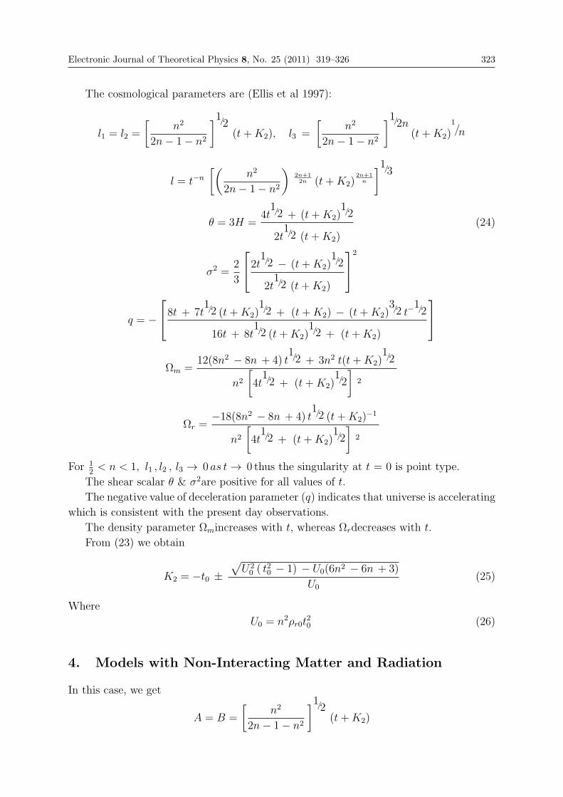
Electronic Journal of Theoretical Physics 8, No. 25 (2011) 319–326 323
The cosmological parameters are (Ellis et al 1997):
l1 = l2 =
[n2
2n− 1− n2
]1/2(t+K2), l3 =
[n2
2n− 1− n2
]1/2n(t+K2)
1/n
l = t−n[(
n2
2n− 1− n2
)2n+12n (t+K2)
2n+1n
]1/3θ = 3H =
4t1/2 + (t+K2)
1/2
2t1/2 (t+K2)
(24)
σ2 =2
3
⎡⎣2t1/2 − (t+K2)1/2
2t1/2 (t+K2)
⎤⎦2
q = −
⎡⎣8t + 7t1/2 (t+K2)
1/2 + (t+K2) − (t+K2)3/2 t−
1/2
16t + 8t1/2 (t+K2)
1/2 + (t+K2)
⎤⎦Ωm =
12(8n2 − 8n + 4) t1/2 + 3n2 t(t+K2)
1/2
n2
[4t1/2 + (t+K2)
1/2
]2
Ωr =−18(8n2 − 8n + 4) t
1/2 (t+K2)−1
n2
[4t1/2 + (t+K2)
1/2
]2
For 12< n < 1, l1 , l2 , l3 → 0 as t→ 0 thus the singularity at t = 0 is point type.
The shear scalar θ & σ2are positive for all values of t.
The negative value of deceleration parameter (q) indicates that universe is accelerating
which is consistent with the present day observations.
The density parameter Ωmincreases with t, whereas Ωrdecreases with t.
From (23) we obtain
K2 = −t0 ±√U20 ( t
20 − 1) − U0(6n2 − 6n + 3)
U0
(25)
Where
U0 = n2ρr0t20 (26)
4. Models with Non-Interacting Matter and Radiation
In this case, we get
A = B =
[n2
2n− 1− n2
]1/2(t+K2)

324 Electronic Journal of Theoretical Physics 8, No. 25 (2011) 319–326
Table 1 : March of the matter density , radiation density, matter-radiation density ratio
and density parameter in the dust model for n = 2/3 ≈ 0.66,t0 = 5 × 10¹⁷ s,ρr0 = 4.67 ×10⁻³⁴ gcm−3, and here K2 = −4.87754× 10¹⁷
Sr.No. t (sec) ρm (g cm−3) ρr (g cm−3) ρm/ρr
1 1018 2.02017249×10⁻³⁵ −1.446723× 10⁻³⁵ −1.396378
2 2.5× 10¹⁸ 3.4657132× 10−36 −9.3751973× 10−37 −3.6966829
3 5× 10¹⁸ 7.1517666× 10−37 −1.8644769× 10−37 −3.8358033
4 7.5× 10¹⁸ 2.9958127× 10−37 −7.7201951× 10−38 −3.8804883
5 1019 1.6372828× 10−37 −4.1954294× 10−38 −3.9025393
6 2.5× 10¹⁹ 1.0071926× 10−38 −6.31795× 10−39 −1.5941763
7 5× 10¹⁹ 6.1239477× 10−39 −1.5485214× 10−39 −3.9547065
8 7.5× 10¹⁹ 2.7069076× 10−39 −6.8373406× 10−40 −3.9590065
Table 2 : March of the matter density , radiation density, matter-radiation density ratio and
density parameter in the dust model for n = 0.9,t0 = 5× 10¹⁷ s,ρr0 = 4.67× 10⁻³⁴ gcm−3, andhere K2 = −1.0574458× 10¹⁰
Sr.No. t (sec) ρm (g cm−3) ρr (g cm−3) ρr + ρm
1 3.5× 10¹⁷ 4.4847777× 10⁻³⁵ −2.4792281× 10⁻³⁵ 2.4792281× 10⁻³⁵
2 4× 10¹⁷ 3.4337823× 10⁻³⁵ −1.8982431× 10⁻³⁵ 1.5355392× 10⁻³⁵
3 4.5× 10¹⁷ 2.7130108× 10⁻³⁵ −1.4997778× 10⁻³⁵ 1.213233× 10⁻³⁵
4 5× 10¹⁷ 2.1975380× 10⁻³⁵ −1.2148196× 10⁻³⁵ 0.9827184× 10⁻³⁵
5 5.5× 10¹⁷ 1.8161465× 10⁻³⁵ −1.0039828× 10⁻³⁵ 0.8121637× 10⁻³⁵
6 7.5× 10¹⁷ 9.766803× 10−36 −5.3991769× 10−36 0.4367626× 10⁻³⁵
7 1018 5.4938288× 10−36 −3.0370376× 10−36 0.2456791× 10⁻³⁵
8 2.5× 10¹⁸ 2.3190129× 10−36 −4.859263× 10−37 0.1833086× 10⁻³⁵
9 3× 10¹⁸ 1.1610427× 10⁻³⁵ −3.3745079× 10−37 1.1272976× 10⁻³⁵
10 3.5× 10¹⁸ 1.1831698× 10−36 −2.4792153× 10−37 .93524827× 10−36
C =
[n2
2n− 1− n2
]1/2n(t+K2)
1/n (27)
Here the two fluids are non-interacting i.e. they obey separate conservation laws. The
conservation of radiation Tij (r); j = 0 leads to
ρr =K3(
n2
2n−1−n2
) 4n+23n (t+K2)
103
(28)
Where K3 is constant of integration.

Electronic Journal of Theoretical Physics 8, No. 25 (2011) 319–326 325
The expression for matter density and pressure are
ρm =3n2 − 2n + 1
n2 (t+K2)2− ρr (29)
pm =1
3
⎧⎨⎩n2 t−3/2(t+K2)
3/2 − 2n2(t+K2) + 2(2n− 1− n2)
2n2 (t+K2)2− ρr
⎫⎬⎭ (30)
And
ρmρr
=(3n2 − 2n+ 1) (n2)
n+23n (t+K2)
43
(2n− 1− n2)4n+23n K3
− 1 (31)
All the cosmological parameters in this case are given by (24), except and which are given
by
Ωm =12t ( 3n2 − 2n + 1)
n2
[4t1/2 + (t+K2)
1/2
]2
− 12t (t+K2)−4/3K3(
n2
2n−1−n2
) 4n+23n
[4t1/2 + (t+K2)
1/2
]2
(32)
Ωr =12t (t+K2)
−4/3K3(n2
2n−1−n2
) 4n+23n
[4t1/2 + (t+K2)
1/2
]2
(33)
Ω0 =12t ( 3n2 − 2n + 1)
n2
[4t1/2 + (t+K2)
1/2
]2
(34)
Conclusion
We have standard observations of anisotropy of the CMB. Here, we have presented power
law solutions of general relativistic two fluid cosmological field equations in Bianchi type
III space time. In both cases we get, point singularity.
We have examined dust ( γ = 1) model in absence of cosmological constant and when
the two fluids are in interacting phase obeying the γ-law equation of state for the matter
field. It is observed that this dust model isotropizes as t → ∞. We have obtained model
in which the deceleration parameter( q) becomes negative for an intermediate period of
time t.
The models presented here are physically meaningful as the associated parameters
behave responsibly, however, they do not reflect the general picture. These are par-
ticular and simple models, nevertheless, our investigation demonstrates the space-time
anisotropy may be an interesting factor to be introduced and investigated to arrive at a
rigorous and reasonable cosmic picture.

326 Electronic Journal of Theoretical Physics 8, No. 25 (2011) 319–326
References
[1] Bali,R, Chandani, N.K. : J. Math. Phys. 49, 032502 (2008).
[2] Coley, A.A., Dunn, K.: Astrophys.J.348, 26(1990).
[3] Coley, A.A.,Tupper, B.O.J.: J.Math. Phys. 27,406(1986).
[4] Collins C.B. and Ellis G.F.R., Phys.Rep. 56,65(1979).
[5] Davidson, W.:Mon.Not. R. Astron. Soc. 124, 79 (1962).
[6] Ellis, G.F.R.: Dynamical Systems in Cosmology. Cambridge University Press,Cambridge (1997).
[7] Harrison, E.: Cosmology. Cambridge University Press. Cambridge (2000).
[8] Kantowaski R. and Sachs R.K., J. Math. Phys. 7,433(1966).
[9] Kristian J. and Sachs R.K., Astrophys.J. 143,379(1966).
[10] McIntosh, C.B.G.:Mon. Not. R. Astron.Soc.140,461(1968).
[11] Pant,D.N.,Oli,S.: Astrophys, Space Sci.281,623(2002).
[12] Roy S.R. and Banerjee S.K., Astrophys. and Space Science 150,213(1988).
[13] Roy S.R. et. al.:Aust.J.Phys.38 ,239(1985).
[14] Sanjay Oli : Astrophys Space Sci 314,89(2008).
[15] Sanjay Oli : Astrophys Space Sci 314,95(2008).
[16] Thorne,K.S.: Astrophysics J. 148,51 (1967).
EJTP 8, No. 25 (2011) 327–342 Electronic Journal of Theoretical Physics
Shell Closures and Structural Information fromNucleon Separation Energies
C. Anu Radha∗, V. Ramasubramanian and E. James Jebaseelan Samuel
School of Advanced Sciences, VIT University, Vellore – 632 014, Tamil Nadu. India
Received 27 April 2010, Accepted 16 January 2011, Published 25 May 2011
Abstract: In this work nuclei along N=Z line are of interest as transitions from spherical
to deformed shapes are expected to occur when going across the medium mass region. In
this respect a strong sudden shape transition between deformation is predicted to occur in
the region N=Z as well as N>Z nuclei. New shell gaps are predicted using nucleon and
two-nucleon separation energies and the shape evaluation are depicted by applying triaxially
deformed cranked Nilsson Strutinsky calculations. Nucleon separation energy plays a major
role in the prediction of new magicity in the proton and neutron drip line nuclei.c© Electronic Journal of Theoretical Physics. All rights reserved.
Keywords: Separation Energy; Stability; Shell Closures; Shape Transition
PACS (2010): 21.10.Gv; 21.10.Dr; 21.10.-k; 21.10.-k; 21.10.Gv
1. Introduction
Nuclear structural calculation far from the region of stability reveals new ideas which are
not usually observed in the stability line. These studies provide information about the
type of decay and the deformation exhibited by the nuclei. Ground state proton emission
is an identification that the drip line has reached. To know about the two proton decay
process, their separation energies need to be calculated. The special quality of proton
rich nuclei is the diproton emission. Due to pairing, a nucleus with an even number of
protons is tightly bound than odd number of proton nucleus [1]. Hence the existence of
two proton emission is sensitive to the two proton separation energies. More number of
nuclei is found to undergo one proton emission either from the ground state or from an
isomeric state or both [2]. When the emitters are found to be deformed, it gives a check
for the nuclear structure models at the drip line [3].
Systematic studies related to nucleon separation energies from the masses of nuclei
328 Electronic Journal of Theoretical Physics 8, No. 25 (2011) 327–342
provide evidence for shell closures. It is important to look for new shell closures or the
disappearance of existing shell closures from the separation energy calculation [4, 5]. The
origin of the unusual stability of nuclei with nucleon numbers 2, 8, 20, 28, 50, 82 and
126, commonly called to as “magic numbers”, is explained to be due to nuclear shell
structure.At present there is a proliferation of new magic or rather quasi-magic numbers
[6, 7]. At the same time some magic numbers are demoted and seem to lose their magicity.
In the simple shell model these are due to shell or sub-shell closures. Shell closure may
be demonstrated by a large drop in separation energies. Such phenomena can be simply
explained by the simple shell model. The single- and two-nucleon separation energies are
fundamental properties of the atomic nucleus [8]. It is a challenge for nuclear many-body
theories to derive the shell model out of complex calculations. Systematic of proton and
neutron separation energies can be powerful tools to study the nuclear structure at and
even beyond the drip lines [9]. It can be used to predict masses and separation energies
of nuclei beyond the neutron and proton drip lines.
This paper is organized as follows. Section 1 is introductory. Section 2 deals with the
theoretical framework used in the study of shell closures and nuclear structure effects.
The found shell gaps, new magicity and shape transitions obtained in the sample case
of fp shell region nucleus titanium isotope are discussed in Sec. 3. The evolution of the
shapes in the rotating titanium isotopes is also traced in Sec.3. Finally, Sec. 4 contains
a summary and conclusion.
2. Theoretical Formalism
An important question in nuclear structure physics is the nature of shape evolution taking
place at critical angular momenta near the limit of stability. In order to know the shape of
the nucleus before fission, this work involves two formalisms. The first framework shows
the nucleon separation energy calculations for various Z and N values in detail. The second
formalism depicts the shape transition in the fp shell region nucleus for evolution of shapes
in the β−γ plane at zero temperature using cranked Nilsson Strutinsky calculations withtuned to fixed spins. The shape transitions details are predicted by using potential energy
surface calculations.
2.1 Separation Energy for sp, sn, s2p, s2n for Different Isotopes and Iso-
tones
Separation energy values for single proton, diproton, single neutron and di neutron are
calculated to show the magicity prevailing in their numbers. The separation energies are
calculated using the relation
S2n(Z,N) = −M(Z,N) +M(Z,N − 2) + 2mn (1)
S2P (Z,N) = −M(Z,N) +M(Z − 2, N) + 2mP (2)
Electronic Journal of Theoretical Physics 8, No. 25 (2011) 327–342 329
In this work, separation energies are calculated for different proton numbers Z for fixed
values of N = 3, 6, 8, 10, 11, 12, 14, 16, 18, 20, 22 and different neutron numbers for
various fixed Z values. The mass value for the daughter nuclei are taken from the Audi
Wapstra mass table [10]. The same work is extended to two proton separation energy
with respect to Z (or N) for fixed neutron (or proton) numbers. Similarly one neutron
and two neutron separation energies are calculated for fixed Z and N values.
2.2 Triaxially Deformed Cranked Nilsson Strutinsky Calculation
The second section gives the theoretical framework for obtaining potential energy surfaces
of the considered nuclei as a function of deformation β and nonaxiality γ parameters at
different spins by the Strutinsky method.
For a non rotating nuclei (zero spin) shell energy calculations assumes a single particle
field
H0 = Σ h0 (3)
where h0 is the triaxial Nilsson Hamiltonian given by
h0 =p2
2m+1
2m
3∑i=1
ω2i x
2i + Cls+D
(l2 − 2
⟨l2⟩). (4)
By Hill-Wheeler parameterization the three oscillator frequencies ωi are given as include
the energy term first
Ek = hωk = hωGDR exp [ -√5/4π β cos (γ – 2/3 Ti K)]
ωx = ω0 exp
(−√
5
4πβ cos
(γ − 2
3π
))
ωy = ω0 exp
(−√
5
4πβ cos
(γ − 4
3π
))
and ωz = ω0 exp(−√
54πβ cos γ
)with the constraint of constant volume for equipotentials
ωxωyωz =◦ω30 = cons tan t (5)
The values [11] for the Nilsson parameters κ and μ are chosen as
κ = 0.093 and μ = 0.15
The value for �ω0 is taken as
�ω0 =45.3 MeV
(A1/3 + 0.77)
. (6)
The same values are used for both protons and neutrons.
The factor 2 in front of 〈l2〉 [Eq. (4)] has been used to obtain better agreement betweenthe Strutinsky-smoothed moment of inertia and the rigid rotor value. The parameter D

330 Electronic Journal of Theoretical Physics 8, No. 25 (2011) 327–342
has been accordingly redetermined with the help of single particle levels in the indicated
mass region. Using the matrix elements, the Hamiltonian is diagonalized in cylindrical
representation up to N=11 shells.
In a rotating nucleus (I �= 0) without internal excitation, the nucleons move in a
cranked Nilsson potential with the deformation described by β and γ. The cranking is
performed around the Z-axis and the cranking frequency is ω. Thus, the Hamiltonian for
a rotating case is given by
Hω = H0 − ωJz =∑
hω (7)
where
hω = h0 − ωjz. (8)
Diagonalization of
�ωφωi = eωi φ
ωi (9)
gives the single particle energy eωi and wave function φωi . The single particle energy in
the laboratory system and the spin projections are obtained as
〈ei〉 = 〈φωi |h◦|φω
i 〉 , (10)
and
〈mi〉 = 〈φωi |jz|φω
i 〉 . (11)
The shell energy is given by
Esp =∑
〈φωi |h◦|φω
i 〉 =∑
〈ei〉 (12)
where
〈ei〉 = eωi + �ω 〈mi〉 . (13)
Thus,
Esp =∑
eωi + �ωI, (14)
with the total spin given by
I =∑
〈mi〉. (15)
To overcome the difficulties encountered in the evaluation of total energy for large defor-
mations through the summation of single particle energies, the Strutinsky shell correction
method is adapted to I �= 0 cases by suitably tuning [12-14] the angular velocities to yield
fixed spins. For unsmoothened single particle level distribution the spin I is given as
I =
λ∫−∞
g2deω =
∑i
〈mi〉 (16)
and
Esp =
λ∫−∞
g1eωdeω + �ωI =
∑i
eωi + �ωI. (17)

Electronic Journal of Theoretical Physics 8, No. 25 (2011) 327–342 331
For the Strutinsky smeared single particle level distribution, Eqs. (16) and (17) transform
in to
I =
λ∫−∞
g2deω =
∑i
〈mi〉 (18)
and
ESP =
λ∫−∞
g1eωdeω + �ωI (19)
=N∑i
eωi + �ωI. (20)
In the tuning method the total spin is adapted and is calculated as
I = Iz =N∑ν=1
⟨Jz
⟩ω
ν+
Z∑π=1
⟨Jz
⟩ω
π. (21)
For a chosen integer or half integer spins the above relation permits to select numerically
the ω values. The calculations are repeated accordingly as the frequency values ω(I)
change from one deformation point to another.
The total energy is given by
ET = ERLDM +(Esp − Esp
)(22)
where
ERLDM = ELDM −1
2Irigω
2 + �ωI . (23)
The liquid drop energy ELDM is given by the sum of Coulomb and surface energies as
ELDM (β, γ) = [2χ (Bc − 1) as + (Bs − 1)] (24)
where Bc and Bs are the relative Coulomb and surface energies of the nucleus. The values
used for the parameters as and χ are as= 19.7 MeV and fissility parameter χ = (Z2/A)/45
where Z and A are the charge and mass numbers of the nucleus.
The rigid body moment of inertia Irig is defined by β and γ including the surface
diffuseness correction and I is the Strutinsky smoothened spin [15]. For an ellipsoidal
shape described by the deformation parameter β and shape parameter γ, the semi axes
Rx,Ry, Rz are given by,
Rx = R0 exp
[√5
4πβ cos
(γ − 2π
3
)]
Ry = R0 exp
[√5
4πβ cos
(γ − 4π
3
)]
and Rz = R0 exp[√
54πβ cos γ
].

332 Electronic Journal of Theoretical Physics 8, No. 25 (2011) 327–342
By volume conservation we have
RxRyRz = R030 (25)
where R00 is the radius of the spherical nucleus. Here,
R00 = r0A
1/3 (r0 = 1.16 fm) . (26)
The moment of inertia about the Z axis is given by
Irig (β, γ) + 2Mb2
�2=1
5
AM(R2
x +R2y
)�
+2Mb2
�2(27)
where 2Mb2 is the diffuseness correction to the moment of inertia and the diffuseness
parameter b = 0.90 fm [16,17,18].
The zero temperature potential energy surfaces for fp shell region isotopes have been
obtained by the tuned Strutinsky procedure. In the calculation performed here the spin
is varied from I = 0� to 30� in steps of 2�, with zero temperature (0.0 MeV), γ from
-180˚ to -120˚ in steps of 10˚, and β from 0.0 to 0.8 in steps of 0.1. The Hill Wheeler
expressions for the frequencies have been used in the cranked Nilsson model [19]. Since
the nuclei considered here 44Ti fall in the region around 28�, for which calculations have
been done for neutron and proton levels separately and shown in the fig.8.
3. Results and Discussions
The fact that all single and two-nucleon separation energies show a similarN/Zdependence
suggests an underlying physical reason for this dependence. It is well-known that separa-
tion energies of isotopic and isotonic nuclei of a given parity type (even–even, even–odd,
odd–even, or odd–odd) follow linear systematic within each shell region if plotted against
Nand Z. The following figures give information about stability and magicity in the light
nuclei. Fig.1 and Fig.2 are respectively plots of S1p for fixed N= 3, 6, 8, 10, 11, 12, 14,
16, 18, 20 and 22 plotted as a function of Z and for fixed Z = 3, 6, 8,10, 11, 12, 14, 16,
18, 20 and 22 plotted as a function of N.
Fig.3 and Fig.4 are respectively plots of S2p for fixed N plotted as a function of Z
and for fixed Z plotted as a function of N. Neutron separation energies are calculated for
fixed isotopes and isotones for varying neutron and proton numbers respectively. Fig.
5 shows the two neutron separation energy variations across the light nuclei and Fig.6
shows the variation of single neutron separation energies with respect to neutron numbers
respectively. It is found that new magic numbers appear and some others disappear in
moving from stable to exotic nuclei in a rather novel manner due to a particular part
of the nucleon-nucleon interaction [20]. We have shown that all single- and two-nucleon
separation energies exhibit a similar N/Z behaviour. Sp vs Z shows that 7N3, 9F6, 17Cl12,
21Sc16 have Sp < 0. Similarly Sp vs.N shows that 10Ne6, 11Na7 and 12Mg8 nuclei are found
to have Sp < 0. For N=Z the separation energy values are found to be higher. Also for

Electronic Journal of Theoretical Physics 8, No. 25 (2011) 327–342 333
Z= 8, N=14 is found to be a magic number. For Z=7 to 9, N=16 is found to be a new
magic number.
Besides the appearance of new shell closures at Z=6, the conventional shell closures
at Z = 20 is on the other hand found to disappear in proton-rich nuclei. A strong kink
has been observed in the lower magic numbers across N = 8 and N = 20. This is clearly
a measure of shell gaps at the magic numbers. Thus the shell gaps provide a sensitive
observable for the shell effects in nuclei. Hence we focus upon Sp and S2p values to explore
the nature of shell effects [21].
When adding protons, asymmetry and Coulomb term reduce the binding energy.
Therefore steeper drop of proton separation energy is observed and the drip line is reached
much sooner. Two-proton separation energies exhibit jumps when crossing magic proton
numbers. The magnitude of the jump is a measure of the proton magic shell gap for a
given neutron number.
It is shown that separation energies disclose rich nuclear structure information. They
indicate very clearly the major shell closures at P = Pmagic or N=Nmagic reflected by
strong discontinuities of Sp, S2p, Sn and S2n as a function of Z and N. The evolution of
nuclear collectivity is reflected as a smooth variation of separation energy as a function
of N or Z [4]. First of all, it shows exactly where are the neutron subshell closures and
its dependence of the proton number; if the major proton spherical shell closures do not
influence the two neutron separation energies, the proton subshell closures due to their
nature (proton-neutron interaction) are reflected in the behavior of separation energies.
A region of extrastability is found at N=6 for proton numbers Z=3-9. Shell closure is
found to be weakened at N=28 in the Z= 15 – 17 region. .
A new shell closure is considered to appear at N=26. A slope change is observed at
Z=8 (oxygen isotope). Similar behaviour is observed at Z=18 also. This change in slope
confirms the possible change in deformation exhibited by those isotopes during decay
clearly shown in fig. 5 having S2n vs N. In the variation of Sn vs N fig. 6 it is found that
there is a loss of magicity for nuclei with N=8. N=6 is found to a new magic number for
Z=3-9 region.
As a sample case just before fission, the shape of the nucleus can be studied from a
titanium isotope. The Fig.7 shows the shape evolution of nucleus from ground state to
various spins till the fission limit in the chosen fp shell region nuclei 44Ti which predicts
the Jacobi shape transition. Fig.8 gives potential energy surfaces of the considered nuclei
as a function of deformation β and nonaxiality γ parameters before fission limit by the
Strutinsky method.
Summary and Conclusion
The paper summarizes the main achievements obtained in the field of the single and
two nucleon emission studies in last years. Another point which is due to the proton-
neutron interaction, the critical point of the transition from spherical to deformed shapes
is reflected in the variation of separation energies but the effect is small. The two proton

334 Electronic Journal of Theoretical Physics 8, No. 25 (2011) 327–342
separation energies and their evolution with neutron and proton number constitute a very
good starting point in testing various nuclear structure models. The analysis presented
in this paper shows the need of very precise data on masses and extension of this type of
information to nuclei very far from stability.
Acknowledgement
The authors thank the VIT University for the support rendered in executing this theo-
retical calculation.
References
[1] A. Abbas, et al Multi nucleon forces and the equivalence of different multi clusterstructures, Mod. Phys. Lett. A16 (2001) 755.
[2] Jorge Rigol, et al “Shell closure at N=164:spherical or deformed”, Phys. Rev.C55(2), (1997), 972.
[3] Sakurai, H. et al Phys.Lett.B 448, (1999) pp 180.
[4] Kanungo, R., et al “Shell closures in the N & Z = 40-60 region for neutron andproton rich nuclei”, Phys. Lett. B649, (2007) 31.
[5] Samanta, C. et al “Extension of the Bethe-Weizasacker mass formula to light nucleiand some new shell closures” Phys.Rev. C 65, (2002) 037301.
[6] Igal Talmi, et al “Old and new quasi magic numbers”, From stable beams toexotic nuclei. AIP Conference Proceedings, 1072, (2008) pp 32.
[7] Sabina Anghel, et al “Structure features revealed from the two neutron separationenergies”, Rom. Journ. Phys., 54, No.3-4, (2009).301.
[8] Sarazin, F. et al “Shape Coexistence and the N=28 Shell Closure Far from Stability”,Hyperfine Interactions 132: 147–152, c© 2001 Kluwer Academic Publishers.
[9] Lidia S. Ferreira, et al “Proton emitting nuclei and related topics”, AIP conferenceproceedings, Portugal, 961, (2007).
[10] G. Audi, A. H. Wapsta and C.Thibault, “The Nubase evaluation of nuclear and decayproperties”, Nucl.Phys. A729 (2003) 337.
[11] Alhassid Y. and Bush B, Nucl. Phys. A 509, (1990), 461.
[12] Shanmugam G., Kalpana Sankar and Ramamurthi K, Phys. Rev. C 52, (1995) 1443.
[13] Shanmugam G., Ramasubramanian V. and Chintalapudi S. N., “Jacobi shapetransition in fp shell nuclei”, Phys. Rev. C 63, (2001) 064311.
[14] Shanmugam G. and Selvam V., “Shape transitions in hot rotating strontium andzirconium isotopes”, Phys. Rev. C 62, (2000) 014302.
[15] G. Vijayakumari and V. Ramasubramanian, Int. J. Pure Appl. Sci., (2008) 36.
[16] Maj A. et al, Nucl. Phys. A 687, (2001a) 192c-197c.
[17] Maj A. et al, Acta Physica Polonica B 32, (2001b) 2433.

Electronic Journal of Theoretical Physics 8, No. 25 (2011) 327–342 335
[18] Maj A. et al, Nucl. Phys. A 731, (2004) 319.
[19] Myers W. D. and Swiatecki W. J., Acta Physica Polonica B 32, (2001) 1033.
[20] C. Anu Radha, “Spherical proton emitters”, M.Phil. Thesis (2005) 97.
[21] C. Anu Radha, E. James Jebaseelan Samuel, “Magicity from separation energies”,DAE Int. Symp. on Nucl.Phys. (2009) 54, 190.

336 Electronic Journal of Theoretical Physics 8, No. 25 (2011) 327–342
Fig. 1 Separation energy Vs. Z for various N values

Electronic Journal of Theoretical Physics 8, No. 25 (2011) 327–342 337
Fig. 2 Separation energy Vs. N for various Z values

338 Electronic Journal of Theoretical Physics 8, No. 25 (2011) 327–342
Fig. 3 Two proton separation energy Vs. Z for various N values
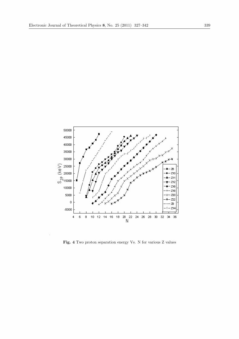
Electronic Journal of Theoretical Physics 8, No. 25 (2011) 327–342 339
Fig. 4 Two proton separation energy Vs. N for various Z values

340 Electronic Journal of Theoretical Physics 8, No. 25 (2011) 327–342
Fig. 5 Two neuton separation energy Vs. N for various Z values

Electronic Journal of Theoretical Physics 8, No. 25 (2011) 327–342 341
Fig. 6 Single neutron separation energy Vs. N for various Z values

342 Electronic Journal of Theoretical Physics 8, No. 25 (2011) 327–342
Fig. 7 Shape evolution of 44Ti for various spin values at zero temperature
Fig. 8 Potential energy surface of 44Ti before fission limit at zero temperature

EJTP 8, No. 25 (2011) 343–352 Electronic Journal of Theoretical Physics
Calculating Vacuum Energy as a PossibleExplanation of the Dark Energy
B. Pan∗†
BABAR Collaboration, Stanford Linear Accelerator Center, 2575 Sand Hill Road,Menlo Park, CA 94025, USA
Received 30 January 2011, Accepted 10 February 2011, Published 25 May 2011
Abstract: We carried out a study of the properties of the λφ4 field solutions. By constructing
Gaussian wave packets to calculate the S matrix, we show that the probability of the vacuum
unbroken state transfers to the broken state is about 10−52. After adding this probability
restriction condition as modulation factor in the summation of vacuum energy, we thus get a
result that the vacuum energy density is about 10−47GeV 4, which is exact same as the observed
dark energy density value, and maybe served as a possible explanation of the dark energy. Also
our result shows that the vacuum energy density is proportional to the square of the universe’s
age, which fits the Dirac large numbers hypothesis.c© Electronic Journal of Theoretical Physics. All rights reserved.
Keywords: Vacuum Energy; Cosmology Constant; φ4, Higgs; Dark Energy
PACS (2010): 95.36.+x; 14.80.Bn
1. Cosmological Constant Problem
In the current standard model of big bang cosmology, the ΛCDM model, dark energy is
a hypothetical form of energy in the space that accelerates the expansion of the universe.
The most recent WMAP [1] [2] observations show that the universe is made up of about
74% dark energy, 22% dark matter, and 4% ordinary matter. The dark energy is measured
in the order of about 10−47GeV 4 [3]. A possible source of the dark energy maybe the
cosmological constant.
The Einstein’s gravity field equation is
Rμν −1
2Rgμν + Λ gμν =
8πG
c4Tμν , (1)
∗ [email protected] or pan [email protected]† Member of the BaBar Collaboration at SLAC of the Stanford university since 2004.

344 Electronic Journal of Theoretical Physics 8, No. 25 (2011) 343–352
in which Λ is the cosmological constant. and it can also be written in the form of vacuum
energy density
ρvacuumc2 =
Λc4
8πG. (2)
The general relativity field equation (1) does not give any physical origin of the
cosmological constant. We may explain it as the zero-point energy of the quantum fields.
In quantum field theory, states can be treated as a set of harmonic oscillators which poses
the zero-point energy
E =∑i
1
2hωi, (3)
which is obviously diverge when sum over all states. If we cut off the summation at the
Planck energy scale EPlank =√
hc3
G� 1019GeV , the zero-point energy density will be
ρ =E4
P lank
4π2h3c5≈ 1074GeV 4, (4)
which is more than 10120 times larger than the measured value of dark energy density.
To cancel almost, but not exactly, the quantum field theory faces a challenge.
In this article, we try to treat the Higgs field energy as the vacuum energy. First we
study the static solution of the λφ4 field equation. Then we figure out the probability of
the vacuum unbroken state transfers to the vacuum broken state. Finally with probability
modulation factor, we calculate the vacuum energy. Our result will be compared to the
experimental data.
2. Solutions of the λφ4 Field
The Lagrangian density of the λφ4 field in the (1+3) dimensions is:
L = −12∂μφ ∂μφ−
μ2
2φ2 − λ
4φ4, (5)
in which φ is the Higgs field, and gμν = (1, 1, 1, 1). The Higgs boson has not been found
yet in experiments, nor does the Standard Model predict its mass. Varies theories and
experiments estimate its mass between 115GeV to 180GeV [3]. In the Standard Model,
with μ2 < 0, the Higgs boson mass is given by mH =√−2μ2 =
√2λ υ, where υ is
the vacuum expectation value of the Higgs field. After spontaneous symmetry breaking,
υ =√−μ2
λ=
√1
2GF≈ 246GeV , fixed by the Fermi weak coupling constant GF . The
vacuum unbroken state has 〈φ〉 = 0, and the vacuum broken state has 〈φ〉 = υ.
From the Lagrangian (5), the equations of motion is
∇2φ− ∂2
∂t2φ = μ2φ+ λφ3, (6)
which can also be written as
∇2
(φ
υ
)− ∂2
∂t2
(φ
υ
)=m2
H
2
⎛⎝(φ
υ
)3
− φ
υ
⎞⎠ , (7)
Electronic Journal of Theoretical Physics 8, No. 25 (2011) 343–352 345
in which mH is the Higgs mass, υ is the broken vacuum expected value.
In one dimension, we know equation (6) has static kink/anti-kink solutions
φ = ±υ tanh(mH
2x). (8)
Because mH ≈ 115 ∼ 180GeV , slope of (8) at x = 0 is
dφ(x)
dx
∣∣∣∣∣x=0
= 2υmH >> 0, (9)
we can replace the 1-dimension kink solution in (8) with a step function in our calculation
without sacrifice accuracy
φ(x) =
⎧⎪⎪⎨⎪⎪⎩υ, when x > 0,
−υ, when x < 0,⇒ φ2(x) = υ2. (10)
By study the properties of the Jacobi elliptic functions sn and cn, we can get other
static solutions of equ. (6) in 1-dimension as
φ(x) = ±υ coth(mH
2x), (11)
φ(x) = ±√2 υ sech(i
mH√2x) = ±
√2 υ sec(
mH√2x) =
±√2 υ
cos(mH√2x), (12)
φ(x) = ±i√2 υ csch(i
mH√2x) = ±
√2 υ csc(
mH√2x) =
±√2 υ
sin(mH√2x). (13)
If φ(x) = F (Ax) is a solution of the equ. (6) in 1-dimension, in which F () is a function
such as listed above in (8), (11), (12), (13) and A is a constant, we can construct (1 + 3)
dimensions solutions of the equ. (6) as
φ(xμ) = F
(A
√aμaμ
(aμxμ)
), (14)
in which aμ are arbitrary constants and automatically sum over μ. For instance, it’s easy
to verify the (1 + 3) dimensions (it, x, y, z) kink-like solution for equ. (6) as
φ(xμ) = ±υ tanh⎛⎝ mH
2√a20 + a21 + a22 + a23
(ia0t+ a1x+ a2y + a3z)
⎞⎠ . (15)
3. Unbroken and Broken States of the Vacuum
The Higgs mechanism requires the vacuum unbroken state has 〈φ〉 = 0, and the vacuum
broken state has 〈φ〉 = υ. Solutions (12) and (13) have domain walls, and can only take
values above +√2 υ or lower than −
√2 υ, which does not fit the 〈φ〉 = 0 requirement of
the unbroken vacuum state. So we will not use them in this calculation.

346 Electronic Journal of Theoretical Physics 8, No. 25 (2011) 343–352
To the solutions (8) and (11), because of their anti-symmetry shape respect to xμ = 0,
both solutions have the property of 〈φ〉 = 0. And because of their asymptotic behavior
at infinity, if xμ goes like 0 → ∞ → 0, then φ(xμ) goes like 0 → υ → ∞. Combination
of the solutions (8), (11) and transform method (14) can let the φ field get values from
−∞ to ∞, which satisfied our requirement. So we will use static 3-dimensions solution
φ(x, y, z) = ±υ tanh⎛⎝ mH
2√a21 + a22 + a23
(a1x+ a2y + a3z)
⎞⎠ (16)
as the initial static state wave function for the unbroken vacuum state. The relation
φ2 ≈ υ2 is still hold even in the 3-dimension case. That the positive or negative sign of
the φ field does not matter, because we will only need φ2 in the following integration.
This approximation greatly reduces the calculation complexity.
To distinguish from the unbroken state φ, we will use ϕ for the spontaneous symmetry
broken vacuum state. We can construct a static local Gaussian packet to represent it,
which is centered at∞ with a narrow width. Or practically to say, it is centered at point
b = (bx, by, bz), in which (bx, by, bz) are the coordinates of point b.
ϕ = υe−Γ2
p((x−bx)2+(y−by)2+(z−bz)2)
2 ei(pxx+pyy+pzz) (17)
in which Γ2p is the packet width in momentum space; px, py, pz are the momentum of the
field; υ reflects the role that equ. (8) and (11) envelope on the Gaussian packet. If values
of each of (bx, by, bz) is very large, ϕ will be very close to υ. In fact, since the slope in (9)
is so large, point b even does not need to be very far away from zero.
4. Packet Width
Follow the reasons in ref. [4], we now try to estimate the width of the Gaussian packet
in equ. (17). By definition, vacuum is the original point for measuring the energy. So
for the unbroken vacuum state, energy Eunbroken = 0. From the Lagrangian(5), we read
out the unbroken vacuum state has m2 = μ2, with μ2 < 0. From the energy-momentum
relation
E2 = p2 +m2, (18)
the momentum will be
p2unbroken = E2unbroken −m2 = −μ2 =
m2H
2. (19)
For the vacuum state after spontaneous symmetry breaking, because we have moved
the original point to 〈φ〉 = υ, the energy will be changed. If we think momentum is
conserved, punbroken = pbroken, and now the broken state has mass square as m2 = m2H =
−2μ2, then
E2broken = p2broken +m2
H =3m2
H
2. (20)

Electronic Journal of Theoretical Physics 8, No. 25 (2011) 343–352 347
From equ. (18), we have EdE = pdp. If we treat dE and dp approximately as ΓE and
Γp for the width of energy and momentum respectively, as explained in detail in ref. [4],
ΓEE = Γpp, (21)
which gives
Γp =Ebroken
pbrokenΓE =
√3ΓE. (22)
[GeV]HM
100 120 140 160 180 200
Bra
nchi
ng ra
tios
-310
-210
-110
1bb
ττ
cc
gg
γγ γZ
WW
ZZ
LHC
HIG
GS
XS W
G 2
010
Fig. 1 List of most significant decay channels branch ratio. (Courtesy from CERN
website [5]).
Fig. 2 Total Higgs width. The dots are simulation results from CMS (Physics TDR) for
the H → ZZ∗ → 4 leptons final state sub-threshold decay. The solid line is the Standard
Model prediction.(Courtesy from Tully’s talk [6]).
Figure (1) summarizes the branching fractions of the most important decay channels
of the Higgs field. The Higgs decay width can be calculated in the Standard Model,
Γ(H → ff) =mH
8π
(mf
υ
)2
Nc
(1−
4m2f
m2H
) 32
,

348 Electronic Journal of Theoretical Physics 8, No. 25 (2011) 343–352
Γ(H → WW ) =m3
H
16πυ2
(1− 4m2
W
m2H
) 12
⎡⎣1− 4
(m2
W
m2H
)+ 12
(4m2
W
m2H
)2⎤⎦ ,
Γ(H → ZZ) =m3
H
32πυ2
(1− 4m2
Z
m2H
) 12
⎡⎣1− 4
(m2
Z
m2H
)+ 12
(4m2
Z
m2H
)2⎤⎦ . (23)
which is plotted in Fig. (2). When mH < 140GeV , the dominant channels is the H → bb,
and the total decay width is in the 10MeV range.
The solid line results in Fig. (2) is arguably for its applicability. When mH is less
than 2mW or 2mZ , we may research the ’sub-threshold decay’, such as H → ZZ∗, whereone Z boson is on-shell and the second Z boson’s mass is off-shell. Simulation from CMS
(Physics TDR) for the H → ZZ∗ →4 leptons final state result is also shown as dots in
Fig. (2) [6] [7]. According to equ. (23), H → WW channel’s width should be a little
greater than H → ZZ. But experimentally, it’s very hard to measure the energy and
momentum of the neutrinos in the H → WW →2 charged leptons + 2 neutrinos case;
compares to the easy be detected one in the H → ZZ →4 charged leptons channel.
Fig. (2) shows the CMS simulation result that, for the Higgs mass around 130GeV ,
ZZ∗ channel sub-threshold decay has Γ � 2GeV . If we think the WW ∗ channel is aboutsame, then the total width for mH = 130GeV is ΓE ≈ 4GeV . That means, from (22),
Γp =√3ΓE ≈ 6.8GeV for mH = 130GeV .
5. Transition Probability of the Vacuum States
The lowest order S matrix involves the transition amplitude of the φ4 interaction, which
made of two incoming vacuum unbroken states φi1φi2 in equ. (16), and two out-going
broken states ϕf1ϕf2 in equ. (17),
Sif =4!
2× 2· λ4〈φi1φi2|ϕf1ϕf2〉
≈ 3λυ2
2
∫ϕf1ϕf2 d
4x
=3π3/2λυ4
2Γ3p
e− p2x+p2y+p2z
Γ2p × phase × displacement×
∫ now
0dt
=3π3/2λυ4T
2Γ3p
e− p2
Γ2p × phase × displacement
= 10−26 × phase, (24)
in which the phase and displacement terms are
phase = ei(px(b1x+b2x)+py(b1y+b2y)+pz(b1z+b2z)),
displacement = exp
[−Γ2p
4
((b1x − b2x)
2 + (b1y − b2y)2 + (b1z − b2z)
2)].

Electronic Journal of Theoretical Physics 8, No. 25 (2011) 343–352 349
The approximate sign in equ. (24) means we replace the square of tanh function with
tanh2 ≈ 1 as in (10). So only the Gaussian integrations of ϕ are left. The phase term
does not contribute to the following probability calculation. So we just omit it. The
displacement term reflects the effect that the two out-going broken states centered at
different points b1 = (b1x, b1y, b1z) and b2 = (b2x, b2y, b2z). We just let them to be at same
points, so the displacement term reaches its maximum value, which is 1. Other values
we used are, υ = 246GeV , λ = m2H/2υ
2 ≈ 1/8, mH = 130GeV , momentum square
p2 = m2H/2 is in equ. (19), Γp =
√3ΓE � 6.8GeV . The time integral gives out a term, T ,
which is the age of the universe, equals to about 1.3×10¹⁰years = 6.2×1041GeV −1. Thenwe get the probability that the vacuum spontaneously transfer from unbroken states to
the broken states,
probability = |Sif |2 = 10−52. (25)
6. Summation over Possible States with Probability
Vacuum does not like matter, in which matter has so many possible states that can
oscillate in many frequencies. The vacuum energy can not contain contributions from
all arbitrary wavelengths, except those physically existed states that are permitted by
the Hamiltonian, e.g. To calculate the summation of states, we made the following
assumptions:
1) The only contribution to the vacuum energy comes from the spontaneous symmetry
breaking, the Higgs mechanism; which means we do not care any other possible sources.
Vacuum has only two states: unbroken state and broken state, which will be the only
two permitted states that appeared in the summation. Because the vacuum unbroken
state has the energy E = 0, so the only state left in the summation is the vacuum broken
state.
2) The summation needs some modulation factor. For instance, to avoid diverge in
the thermal radiation expression, in the derivation of the Planck’s formula of blackbody
radiation, we not only add up the energy of photons, but also times the Bose-Einstein
distribution factor 1/(ehνkT − 1). In this paper, we chose the probability of the transition
from unbroken state to the broken state as the suppression factor.
Finally we sum the energy in phase space and get the vacuum energy density,
ρ =4πp2dp · E(2π)3
× probability = 10−47GeV 4, (26)
in which the momentum and energy are in equ. (19) and (20), ≈ (1 to 2) × 102GeV ;
dp ≈ Γp; probability term is in equ. (25). It is amazing to see that our result in (26) is
exact same as the value that observed in the experiments.

350 Electronic Journal of Theoretical Physics 8, No. 25 (2011) 343–352
7. Discussion
By adding certain conditions in the calculation of the vacuum energy, we get a same
result to the observed value and maybe served as a possible explanation of the dark
energy. Higgs has not been found yet in any experiment. The numerical estimation of
the transition probability is sensitive to the input mass and width value. So we need
further experimental data to consolidate out calculation.
When we integrate the S matrix as transition amplitude, we use static wave functions.
It maybe asked why we have E, ΓE, p and Γp, but only e−Γ2
px2and eipx appeared in the
calculation expression, while e−ΓEt and e−iEt did not show up? A possible explanation
is that E is only occurred after symmetry breaking. Its value affects the decay after
symmetry breaking, but not related to the unbroken state.
The Dirac large numbers hypothesis [8] [9] [10], made by Paul Dirac in 1937, proposed
relations of the ratios between some fundamental physical constants. The hypothesis has
two important consequences:
1) Matter should be continuously created with time. The mass of the universe is
proportional to the square of the universe’s age: M ∝ T 2. According to Dirac, the
continuous creation of mass maybe either of two models. Additive creation, assumes
that matter is created uniformly throughout space. Or multiplicative creation, created
of matter where matter already exists and proportion to the amount already existing.
2) The gravitational constant, G, is inversely proportional to the age of the universe:
G ∝ 1/T .
In our analysis, the transition amplitude (24) proportions to T , means that the vac-
uum energy density in equ. (26) has the character of ρ ∝ T 2, in which T is the age of the
universe. Since the dark energy is about 74% of the universities mass, we can roughly
to say that equ. (26) fits the consequence of the Dirac large numbers hypothesis, in case
we did not count the expansion of the universe. If our calculation is correct, this relation
will have a serious effect on the evolution of the universe.
References
[1] N. Jarosik, et al., Astrophys. J. Suppl. Ser. 192, 14(2011); arXiv:1001.4744.
[2] G. Hinshaw, et al. (WMAP Collaboration), Astrophys. J. Suppl. Ser. 180, 225 (2009);arXiv:0803.0732.
[3] K. Nakamura, et al. (Particle Data Group), Review of Particle Physics 2010,http://www-pdg.lbl.gov.
[4] E. Kh. Akhmedov, A. Yu. Smirnov, Phys. Atom. Nucl. 72 1363 (2009);arXiv:0905.1903.
[5] https://twiki.cern.ch/twiki/bin/view/CMSPublic/WebHome.
[6] C. Tully, Searching for the Higgs,http://www.slac.stanford.edu/econf/C060717/lec notes/Tully072406.pdf.
[7] M. Kado, C. Tully, Annu. Rev. Nucl. Sci. 52, 65 (2002).

Electronic Journal of Theoretical Physics 8, No. 25 (2011) 343–352 351
[8] P. Dirac, Nature 139 323 (1937). doi:10.1038/139323a0.
[9] P. Jordan, Nature 164 637 (1949).
[10] Saibal Ray, Utpal Mukhopadhyay, Partha Pratim Ghosh, arXiv:0705.1836.


EJTP 8, No. 25 (2011) 353–360 Electronic Journal of Theoretical Physics
Some Bianchi type-I Cosmic Strings in a Scalar–Tensor Theory of Gravitation
R.Venkateswarlu1, J.Satish2 and K.Pavan Kumar3∗
1GITAM School of International Business, GITAM University, Visakhapatnam 530045,India
2Vignan’s Institute of Engineering for Women, Duvvada, Vadlapudi, Visakhapatnam530046, India
3Swarnandhra College of Engg. & Tech, Narsapur 534 280, India
Received 6 July 2010, Accepted 10 February 2011, Published 25 May 2011
Abstract: The field equations are obtained in Sen–Dunn theory of gravitation with the help
of LRS Bainchi type-I in the context of cosmic strings. We have solved the field equations when
the shear σ is proportional to the scalar expansion θ. It is found that the cosmic do not exist
with the scalar field except for some special cases and hence vacuum solutions are presented
and discussed.c© Electronic Journal of Theoretical Physics. All rights reserved.
Keywords: Gravitation; General Relativity; Bianchi type-I
PACS (2010): 95.30.Sf; 04.20.-q
1. Introduction
Brans and Dicke [1] have formulated a scalar-tensor theory of gravitation in which the
tensor field alone is geometrised and the scalar field is alien to the geometry. Sen and
Dunn [2] have proposed a new scalar-tensor theory of gravitation in which both the scalar
and tensor fields have intrinsic geometrical significance. The scalar field in this theory is
characterized by the function φ = φ(xi) where xi are coordinates in the four – dimensional
Lyra manifold and the tensor field is identified with the metric tensor gijof the manifold.
The field equations given by Sen and Dunn for the combined scalar and tensor fields are
Rij −1
2gijR = ωφ−2(φ,iφ,j −
1
2gijφ,kφ
,k)− φ−2Tij (1)
∗ rangavajhala [email protected]

354 Electronic Journal of Theoretical Physics 8, No. 25 (2011) 353–360
where ω = 32, Rij and R are respectively the usual Ricci-tensor and Riemann-curvature
scalar (in our units C = 8πG = 1).
Sen-Dunn [3], Halford [4], Singh [5], Reddy [6, 7], Roy and Chatterjee [8, 9], and
Reddy and Venkateswarlu [10]are some of the authors who have studied various aspects
of this scalar-tensor theory of gravitation.
In recent years there has been lot of interest in the study of cosmic strings. Cosmic
strings have received considerable attention as they are believed to have served in the
structure formation in the early stages of the universe. Cosmic strings may have been
created during phase transitions in the early era [11] and they act as a source of grav-
itational field [12]. It is also believed that strings may be one of the sources of density
perturbations that are required for the formation of large scale structures of the universe.
The energy momentum tensor for a cloud of massive strings that can be written as
Tij = ρuiuj − λxixj. (2)
Here ρ is the rest energy density of the cloud of strings with particles attached to them,
λ is the tension density of the strings and ρ = ρp + λ, ρp being the energy density of the
particles. The velocity ui describes the 4 – velocity which has components (1, 0, 0, 0) for
a cloud of particles and xi represents the direction of string which will satisfy
uiui = −xixi = 1 and uixi = 0. (3)
The study of cosmic strings in relativistic framework was initiated by Stachel [13] and
Letelier [14]. Krori et.al. [15, 16], Raj Bali and Shuchi Dave [17], Bhattacharjee and
Baruah [18], Mahanta and Abhijit Mukharjee [19], Rahaman et al. [20], Reddy [21], Pant
and Oli [22], Venkateswarlu et al. [23] and Venkateswarlu and Pavan [24] are some of
the authors who have studied various aspects of string cosmologies in general relativistic
theory as well as in alternative theories of gravitation.
In this paper, we made an attempt to solve the LRS Bianchi type-I field equations
in the context of cosmic strings in a new scalar-tensor theory of gravitation proposed by
Sen and Dunn [2].
2. Metric and Field Equations
We consider the LRS Bianchi type –I metric as
ds2 = −dt2 + A2dx2 +B2(dy2 + dz2) (4)
where A and B are functions of t only .
The field equation (1) for the metric (4) are given by
2B44
B +
B24
B2= φ−2λ+
ω
2
(φ4
φ
)2
(5)
A44
A+B44
B+A4B4
AB=ω
2
(φ4
φ
)2
(6)

Electronic Journal of Theoretical Physics 8, No. 25 (2011) 353–360 355
2A4B4
AB+B2
4
B 2= φ−2ρ− ω
2
(φ4
φ
)2
(7)
where the subscript 4 denotes ordinary differentiation with respect to t.
3. Solutions to the Field Equations
The field equations (5) – (7) are a system of three equations with five unknown parameters
A, B,φ, ρ and λ. We need two additional conditions to get a deterministic solution of
the above system of equations. Thus we present the solutions of the field equations in
the following physically meaningful cases:
Case 1: We assume the following two conditions:
(i) The shear σ is proportional to the scalar expansion θ which leads to
B = Am (8)
where m is a constant and
(ii)
ρ = λ(geometric strings). (9)
Now the field equations (5) - (7) together with (8) and (9) reduces to
A44
A+ 2m
A 24
A 2= 0 (10)
which on integration yields
A(t) = [(2m+ 1)(C1t+ C2)]1
(2m+1) (11)
and from (8)
B(t) = [(2m+ 1)(C1t+ C2)]m
(2m+1) (12)
where C1 and C2 are constants of integration.
From equation (6) the scalar field is given by
φ = (C1t+ C2)k (13)
where k =[− 2m(m+2)
ω(2m+1)2
]1/2and m < −2.
By making use of equations (11), (12) and (13) in equations (5) and (7), the string
energy density ρ and the tension density λ become zero. Hence it is observed that cosmic
geometric strings do not co-exist with the scalar field in this theory.
When m = −1, the vacuum solution of the field equations (5)-(7) can be written as
(after suitably redefining the constants)
A(t) =1
t(14)
B(t) = t (15)

356 Electronic Journal of Theoretical Physics 8, No. 25 (2011) 353–360
and the scalar field takes the form
φ(t) = t√2√ω (16)
Case 2: The p-strings or Takabayasi strings are represented by ρ = (1 + ξ)λ, ξ >0. In
this case, the field equations (5) – (7) along with equation (8) reduced to
[ξ(1−m) + 2]A44
A+ 2m[ξ(1−m) + 2]
A24
A2= 0 (17)
Equation (17) is formerly similar to equation (10) and hence its solution is also similar
to the one given by equations (11), (12) and (13). Thus in this case the p-strings do not
co-exist with the Sen – Dunn’s scalar field.
Case 3: In this case we consider the condition given by equation (8) together with
ρ+ λ = 0. The solution of the field equations (5) – (7) together with (8) is similar to the
solution obtained in case (1) and it is also observed that the non-existence of the scalar
field in this theory.
Case 4: To get a realistic solution here we assume that
A = A0tm and B = B0t
n (18)
where A0, B0,m and n are arbitrary constants. Then from equation (6) we obtain
φ = φ0tk (19)
where φ0 is an arbitrary constant and k =(
2(m2+n2+mn−m−n)ω
) 12.
Thus the LRS Bianchi type-I model can be written as (after suitably redefining the
constants)
ds2 = −dt2 + t2m dx2 + t2n(dy2 + dz2). (20)
The string energy density ρ, tension density λ, the particle density ρp, the scalar expansion
θ, the shear scalar σ, spatial volume V and the deceleration parameter q are given by
ρ = φ 20
(m+ n)(m+ 2n− 1)
t2−2k(21)
λ = φ20
(n−m)(m+ 2n− 1)
t2−2k(22)
ρp = ρ− λ =2φ 2
0m(m+ 2n− 1)
t2−2k. (23)
θ =(m+ 2n)
t(24)
σ =(m− n)√
3 t(25)
V = t(m+2n) (26)
q =(3−m− 2n)
(m+ 2n)(27)

Electronic Journal of Theoretical Physics 8, No. 25 (2011) 353–360 357
The energy conditions viz.,ρ > 0, λ > 0 and ρp > 0 are identically satisfied for all m > 0
and n > 0. Since σθ= constant, the model given by equation (20) does not approach
isotropy at any stage. The spatial volume of the model increases with the increase in
time. The model given by equation (20) for a cloud of cosmic strings possess a line
singularity as ρ, λ, θ and σ tend to infinity and spatial volume tend to zero at initial
epoch t = 0. When m = n, it is interesting to note that λ = 0 which corresponds to dust
filled isotropic universe without strings.
Case 4.1 : The case ρ = λ refers to geometric strings. Here we have either m = 0
and m = 1− 2n. If m = 0, the solution of the field equations (5)-(7) is given by
A = Constant, B = B0tn (28)
and the scalar field
φ = φ0 tk1 (29)
where k1 =(
2(n2−n)ω
) 12.
The string energy density ρ and tension density λ are
λ = ρ = φ20
(2n2 − n)
t2−2k. (30)
When m = 1− 2n, the string energy density ρ and tension density λ become zero.
Case 4.2 : Now we consider the case ρ + λ = 0 i.e., the sum of rest energy density
and tension density for cloud of strings vanish. Then we have either n = 0 and n = 1−m2.
When n = 0, the solution of the field equations (5)-(7) can be expressed as
A = A0tm and B = Constant (31)
and the scalar field is given by
φ = φ0 tk2 (32)
where k2 =(
2(m2−m)ω
) 12.
The string energy density ρ and tension density λ are
λ = −ρ = φ20
(m2 −m)
t2−2k. (33)
Again if n = 1−m2, λ = ρ = 0 this shows that the cosmic strings do not exist.
It is observed that the scalar field becomes a constant in both the cases i.e., when m
= 1, n = 0 or m = 0, n = 1. These situations lead to the general relativity case.
Case 4.3 : The p-strings or Takabayasi strings are represented byρ = (1+ξ)λ, ξ >0.
Now the string energy density ρ, tension density λ, and the particle density ρp are given
by
ρ = φ20
(m+ n)(m+ 2n− 1)
t2−2k(34)
λ = φ20
2m(m+ 2n− 1)
ξ t2−2k(35)

358 Electronic Journal of Theoretical Physics 8, No. 25 (2011) 353–360
ρp = ρ− λ =φ 20 (m+ n− 2m/ξ)(m+ 2n− 1)
t2−2k.
where the constants m, n and ξ are related by n = 2+ξξm . It is evident that the energy
conditions viz.,ρ > 0, λ > 0 and ρp > 0 are identically satisfied for all m > 0 and n > 0.
In this case we observed that the p-strings or Takabayasi strings do exist in a new
scalar-tensor theory of gravitation proposed by Sen – Dunn.
Conclusions
We obtained the field equations of Sen – Dunn theory of gravitation with the help of
LRS Bianchi type-I metric in the context of cosmic strings. The solutions of the field are
discussed in various physically meaningful cases. It is observed that the cosmic strings
do not co- exist when the shear scalar is proportional to the scalar of expansion. We also
noticed that the cosmic strings do exists when the metric potentials are given by equation
(17). Again for specific values of m and n, strings do not co – exist in Sen – Dunn theory
of gravitation.
References
[1] Brans, C and Dicke ,R. H.: Phys.Rev.124,925 . (1961)
[2] Sen, D. K and Dunn, K. A J. Math. Phys.13, 557. (1971)
[3] Dunn K, A. J. Math. Phys .15, 2229. (1974)
[4] Halford W. D. J. Math. Phys.13, 1699 . (1972)
[5] Singh, T. J. Math. Phys.16, 2109 . (1975)
[6] Reddy, D. R. K. J. Phys. A: Math. Nucl. Gen .6, 1867. (1973)
[7] Reddy, D. R. K. J. Math. Phys. 20, 23. (1979)
[8] Roy A. R. and Chattterjee,B. Acta Phys. Hung. 48, 383. (1980)
[9] Roy A. R . and Chattterjee, B. Indian J. Pure Appl.Math. 12, 659. (1981)
[10] Reddy, D. R. K. and Venkateswarlu: Astrophys. Space Sci. 135, 287 (1987)
[11] Kibble, T. W. B.: J. Phys. A 9, 1387 (1976)
[12] Letelier, P. S.: Phys. Rev. D 28, 2414 (1983)
[13] Stachel, J.: Phys. Rev. D 28, 2171 (1990)
[14] Letelier, P. S.: Phys. Rev. D 20, 1294 (1979)
[15] Krori, K. D., Choudhury, T., Mahanta, C. R.: Gen. Relativ. Gravit. 22, 123 (1990)
[16] Krori, K. D., Choudhury, T., Mahanta, C. R.: Gen. Relativ. Gravit. 26, 265 (1994)
[17] Bali, R., Dave, S.: Pramana, J. Phys. 56, 4 (2001)
[18] Bhattacharjee, R., Baruah, K. K.: Indian J. Pure Appl. Math. 32, 47 (2001)

Electronic Journal of Theoretical Physics 8, No. 25 (2011) 353–360 359
[19] Mahanta, Mukharjee, A.: Indian J. Pure Appl. Math. 32, 199 (2001)
[20] Rahaman, F., Chakraborty, S., Das, S., Hossain, M., Bera, J.: Pramana, J. Phys.60, 453 (2003)
[21] Reddy, D.R.K.: Astrophys. Space Sci. 286, 359 (2003)
[22] Pant, D.N., Oli, S.: Pramana, J. Phys. 60, 433 (2003)
[23] Venkateswarlu, R., Pavan Kumar, K., Rao, V.U.M.: Int. J. Theor. Phys. 47, 640(2008)
[24] Venkateswarlu, R., Pavan Kumar, K.,: Int. J. Theor. Phys. 49, 1894(2010).


EJTP 8, No. 25 (2011) 361–378 Electronic Journal of Theoretical Physics
Gravitons Writ Large; I.E. Stability, Contributionsto Early Arrow of Time, and Also Their PossibleRole in Re Acceleration of the Universe 1 Billion
Years Ago?
A. Beckwith∗
Institute of Theoretical Physics,Department of Physics, Chongquing University, ChinaAmerican Institute of Beamed Energy Propulsion†, Seculine Consulting, USA
Received 6 July 2010, Accepted 10 February 2011, Published 25 May 2011
Abstract: This document is due to a question by Debasish of the Saha institute of India
asked in the Dark Side of the Universe conference, 2010, in Leon, Mexico, and also is connected
with issues as to the initial configuration of the arrow of time brought up in both Rudn 10, in
Rencontres de Blois, and Fundamental Frontiers of Physics 11, in Paris, in July 2010. Further
reference is made as to how to reconcile early inflation with re acceleration, partly by dimensional
analysis and partly due to recounting a suggestion as by Yurov, which the author thinks has
merit and which ties into, to a point with using massive gravitons as a re acceleration of the
universe a billion years ago enabler, as perhaps a variant of DE.c© Electronic Journal of Theoretical Physics. All rights reserved.
Keywords: cosmology; Early Universe; Arrow of Time; Gravitons
PACS (2010): 98.80.-k; 98.80.Cq; 14.70.Kv
1. Introduction
The supposition advanced in this article is that relic energy flux initially is central to
making predictions as to verifying Sentropy ∼ nf [1,2,6,7], where nf is a ‘particle count’
per phase space ‘volume’ in the beginning of inflation. Having said that, is nf due
to gravitons in near relic conditions? Or is Sentropy ∼ nf due to coherent clumps of
gravitons? If so, can the gravitons/ coherent clumps of gravitons carry information ? The
author in previous manuscripts [1,2] identified criteria as to Sentropy ∼ nf |start−of−inf ∝105 ⇔ initial information ∝ 107 bits of ‘information’ in line with G. Smoot’s Paris (2007)
∗ [email protected], [email protected]† www.iibep.org

362 Electronic Journal of Theoretical Physics 8, No. 25 (2011) 361–378
[8] talk as presented in the Paris Observatory. Having said that, the relevant issue
as raised in DSU 2010, if gravitons with a small mass are part of the bridge between
Sentropy ∼ nf |start−of−inf ∝ 107 ⇔ initial information ∝ 1010 bits of ‘information’ , can
one make a statement about necessary conditions for ‘massive’ graviton stability ? Next,
if there is a mass associated with What can be said about massive graviton stability ?
We look at work presented by Maggiorie [9] which specifically delineated for non zero
graviton mass, where h ≡ ηuvhuv = Trace · (huv) and T = Trace · (T uv) that
−3m2gravitonh =
κ
2· T (1)
Our work uses Visser’s [10] 1998 analysis of non zero graviton mass for both T and h.
We will use the above equation with a use of particle count nf for a way to present initial
GW relic inflation density using the definition given by Maggiore [9] as a way to state
that a particle count
Ωgw ≡ρgwρc≡
f=∞∫f=0
d(log f) · Ωgw (f)⇒ h20Ωgw (f) ∼= 3.6 ·[ nf
1037
]·(
f
1kHz
)4
(2)
where nf is the frequency-based numerical count of gravitons per unit phase space. To
do so, let us give the reasons for using Visser’s [10] values for T and h above, in Eq. (1).
While Maggiore’s explanation [9] , and his treatment of gravitational wave density is
very good, the problem we have is that any relic conditions for GW involve stochastic back
ground, and also that many theorists have relied upon either turbulence/ and or other
forms of plasma induced generation of shock waves, as stated by Duerrer, et. al.[11] and
others looking at the electro weak transition as a GW generator. If relic conditions can
also yield GW / graviton production, and the consequences exist up to the present era,
as Beckwith presented, then the question of stability of gravitons is even more essential
Beckwith write up an early energy flux for GW/ gravitons which he wrote as [ 13]
.
Einitial−flux ∼=[r2
64π
]·∣∣+∂2rh+∣∣2 · [n · tPlanck]
3 · Ωeffective (3)
The nf value obtained, was used to make a relationship , using Y. J. Ng’s entropy [
6 ] counting algorithm of roughly Sentropy ∼ nf . We assert that in order to obtain
Sentropy ∼ nf from initial graviton production, as a way to quantify nf , that a small mass
of the graviton can be assumed. A small mass graviton in four dimensions only makes
sense if it is a stable construct. The remainder of this article will be in giving specific
cases as to criteria for stability for the low mass 4 dimensional graviton assumed by the
author in obtaining his value of Sentropy ∼ nf [1,2,3,6,8] and resultant information content
present in the early universe. In doing so, the author will address if the correspondence
principle and the closeness of the links to massless formalism of the graviton as will be
brought up is due to ‘tHoofts [ 12, 13, 14 ] idea of an embedding of QM within what he
calls deterministic quantum theory, involving an embedding of quantum physics within
a slightly ‘larger’ highly non linear structure.

Electronic Journal of Theoretical Physics 8, No. 25 (2011) 361–378 363
1.1 Defining the Graviton Problem and Using Visser’s (1998) Inputs into
Tuv
We begin our inquiry by initially looking at a modification of what was presented by R.
Maartens [15] , as done by Beckwith [12,13]
mn(Graviton) =n
L+ 10−65grams (4)
On the face of it, this assignment of a mass of about 10−65 grams for a 4 dimensional gravi-ton, allowing for m0(Graviton − 4D) ∼ 10−65grams[‘12,13] violates all known quantummechanics, and is to be avoided. Numerous authors, including Maggiore [9] have richly
demonstrated how adding a term to the Fierz Lagrangian for gravitons, and assuming
massive gravitons leads to results which appear to violate field theory, as we can call it .
Turning to the problem, we can examine what inputs to the Eqn. (1) above can tell us
about if there are grounds for m0(Graviton− 4D) ∼ 10−65grams [12,13] , and what thissays about measurement protocol for both GW and gravitons as given in Eqn. (2) above.
Visser [10] , in 1998 came up with inputs into the GR stress tensor and also , for the
perturbing term huv which will be given below. We will use them to perform a stability
analysis of the consequences of setting the value of m0(Graviton − 4D) ∼ 10−65grams[10,12,13], and discuss how T’Hooft’s [12,13,14] supposition of deterministic QM, as an
embedding of QFT, and more could play a role if there are conditions for stability of
m0(Graviton− 4D) ∼ 10−65grams [10,12, 13]
1.2 Visser’s treatment of the Stress Energy Tensor of GR, and its Appli-
cations
Visser[10] in 1998, stated a stress energy treatment of gravitons along the lines of
Tuv|m �=0 =
[(�
l2Pλ2g
)·(GM
r
)· exp
(r
λg
)+
(GM
r
)2]×
⎡⎢⎢⎢⎢⎢⎢⎢⎣
4 0 0 0
0 0 0 0
0 0 0 0
0 0 0 0
⎤⎥⎥⎥⎥⎥⎥⎥⎦(5)
Furthermore, his version of guv = ηuv + huv can be written as setting
huv ≡ 2GM
r·[exp
(−mgr
�
)]· (2 · VμV ν + ηuv) (6)
If one adds in velocity ‘reduction’ put in with regards to speed propagation of gravitons
[10]
v=g c ·√1−
m2g · c4�2ω2
g
(7)

364 Electronic Journal of Theoretical Physics 8, No. 25 (2011) 361–378
As well as setting (MG/r) ≈ 1/5for reasons which Visser[10] outlined, one can obtain a
real value for the square of frequency > 0, i.e.
�2ω2 ∼= m2
gc4 · [1/(1− A)] > 0 (8)
A =
{1− 1
6mgc2
(�2
l2Pλ2g
· exp[− r
λg+mg · r�
]+
(MG
r
)· exp
(mgr
�
))}2
(9)
According to Jin Young Kim [16] , if the square of the frequency of a graviton, with
mass, is >0, and real valued, it is likely that the graviton is stable, at least with regards
to perturbations. Kim’s article [16] is with regards to Gravitons in brane / string theory,
but it is likely that the same dynamic for semi classical representations of a graviton with
mass.
1.3 Conditions Permitting Eqn (8) to have Positive Values
Looking at Eqn. (1.8) is the same as looking at the following, analyzing how
A =
{1− 1
6mgc2
(�2
l2Pλ2g
· exp[− r
λg+mg · r�
]+
(MG
r
)· exp
(mgr
�
))}2
< 1 (10)
I.e. setting
0 <1
6mgc2
(�2
l2Pλ2g
· exp[− r
λg+mg · r�
]+
(MG
r
)· exp
(mgr
�
))< 1 (11)
Note that Visser [10] (1998) writes mg < 2 × 10⁻²⁹eV ∼ 2 × 10−38mnucleon, and a wave
length λg ∼ 6 × 10²²meters. The two values, as well as ascertaining when one can useMGr∼ 1/5, with r the usual distance from a graviton generating source, and M the mass’
of an object which would be a graviton emitter put severe restrictions as to the volume
of space time values for which r could be ascertained. If, however, Eq. (10) had, in most
cases, a setting for which, then in many cases, Eq. (1.8) would hold.
0 ≤ exp
[− r
λg+mg · r�
]<< 1 (12)
The author believes that such a configuration would be naturally occurring in most
generation of gravitons at, or before the Electro Weak transition point in early cosmology
evolution.
1.4 Review of if there is a nf ≈ 105to · 106 Initial Production of CoherentGroups of Gravitons in Relic Conditions. And its effect on the arrow
of time question
The author, Beckwith, believes, that satisfying Eqn. (12) would allow to predict a particle
count behavior along the lines where Beckwith[1,2,3] obtained nf ≈ 105to·106. This value

Electronic Journal of Theoretical Physics 8, No. 25 (2011) 361–378 365
of nf ≈ 105to · 106 as given by Beckwith[1,2,12,13] would be put into Eqn. (2) above,
which would have implications for what to look for in stochastic GW generation. The
question to raise, is what “particle” is being counted, in nf ≈ 105to · 106. Conceivably,it could be coherent packets of gravitons. The reasons for raising this question will be
spelled out in the following analysis.
Recently, Beckwith asked [1,2,3] if the following could occur, S ≡ [E − μN ]/T → S ∝T 3 by setting the chemical potentialμ → 0with initial entropy S ∼ 105 at the beginning
of inflation . Conventional discussions of the arrow of time states that as the Universe
grows its temperature drops, which leaves less energy available to perform useful work
in the future than was available in the past. Thus the Universe itself has a well-defined
thermodynamic arrow of time. The problem of the initial configuration of the arrow of
time, however, is not brought up. This paper is to initiate how to set up a well defined
initial starting point for the arrow of time. Specifically re setting the degrees of freedom
of about g∗ ∼ 100−120[1,2,3] of the electro weak era, to g∗ ∼ 1000at the onset of inflation
[1] , may permit Sinitial ∝ T 3. If the initial temperature of an emerging universe were
very low, scaling S ∝ T 3may be a way to get an arrow of time, with respect to thermal
temperatures, alone, with the graviton count a later, emergent particle phenomenon.
2. What can be Said Initially about Usual Arrow of Time For-
mulations of Early Cosmology?
Usual treatments of the arrow of time, i.e. the onset of entropy . The discussion below
makes the point that expansion of the universe in itself does not ‘grow’ entropy
The entropy density s of a radiation field of temperature T is s ∼ T3. The entropy
S in a given comoving volume V is S = sV . Since the commoving volume V increases
as the universe expands, we have V ∼ R 3. And since the temperature of the microwave
background goes down as the universe expands: T ∼ 1/R, we have the result that the
entropy of a given comoving volume of given space S ∼ R −3 * R3 = constant. Thus
the expansion of the universe by itself is not responsible for any entropy increase. There
is no heat exchange between different parts of the universe. The expansion is adiabatic
and isentropic: dS expansion = 0. I.e. a process has to be initiated in order to start
entropy production
This discussion above is to emphasize the importance of an initial process for the
onset and the growth of entropy. We will initiate candidates for making sense of the
following datum
To measure entropy in cosmology we can count photons. If the number of photons in
a given volume of the universe is N, then the entropy of that volume is S ∼ kN where k
is called here Boltzmann’s constant
Note that Y. Jack Ng. has [6] , from a very different stand point derived S ∼ nbased
upon string theory derived ideas , with n a ‘particle’ count , which in Y. Jack Ng’s
procedure is based upon the number of dark matter candidates in a given region of phase
space..Y. Jack Ng’s idea was partly based upon the idea of quantum ‘ infinite ‘ statistics,

366 Electronic Journal of Theoretical Physics 8, No. 25 (2011) 361–378
and a partition function..
This counting procedure is different from traditional notions . To paraphrase them,
one can state that “The reason why entropy is increasing is because there are stars in
that “box” ( unit of phase space used for counting contributions to entropy). Hydrogen
fuses to helium and nuclear energy is transformed into heat.” I.e. the traditional notion
would be akin to heat production due to, initially start BBN nucleosynthesis, and then,
frankly , star production/ nuclear burning. I.e. one would need to have nuclear processes
to initiate heat production. This idea of heat production is actually similar to setting
S ∝ T 3, with heat production due to either BBN/ hydrogen burning leading to an increase
in temperature, T. In this manuscript, we make use of, if S ≡ [E − μN ]/T → S ∝ T 3
by setting the chemical potentialμ → 0with initial entropy S ∼ 105 at the beginning of
inflation. This entails, as we will detail , having increased number of degrees of freedom,
initially, with re setting the degrees of freedom of about g∗ ∼ 100 − 120of the electro
weak era, to g∗ ∼ 1000at the onset of inflation, I.e. what will be examined will be the
feasibility of the following: S ≡ [E − μN ]/T −→μ→0
S ∝ T 3 ≈ n, with n an initial ‘quantum
unit’ count in phase space of Planckian dimensions, where S ∼ 105 at the beginning of
inflation. Let us now look at how to initiate such a counting algorithm if one is looking
at , say, highly energized gravitons , initially, as part of a counting ‘algorithm’.
2.1 Estimating the Size of Contribution to Energy in S ≡ E/T , Assuming
a Peak Frequency ν ∼ 1010 Hertz for Relic Gravitons, if the Standard
Chemical Potential is Effectively μ = 0 at the Onset of Creation
As suggested earlier by Beckwith [12,13], gravitons may have contributed to the re-
acceleration of the universe one billion years ago. Here, we are making use of refining the
following estimates. In what follows, we will have even stricter bounds upon the energy
value (as well as the mass) of the graviton based upon the geometry of the quantum
bounce, with a radii of the quantum bounce on the order of lP lanck ∼ 10−35meters [1], [5].
mgraviton|RELATIV ISTIC < 4.4× 10⁻²²h−1eV/c2
⇔ λgraviton ≡ �
m·gravitonc< 2.8× 10⁻⁸meters
(13)
For looking at the onset of creation, with a bounce; if we look at ρmax ∝ 2.07 · ρplanck forthe quantum bounce with a value put in for when ρplanck ≈ 5.1 × 1099grams/ meter3,
where [1]
Eeff ∝ 2.07 · l3Planck · ρplanck ∼ 5× 1024GeV (14)
Then, taking note of this , one is obtaining having a scaled entropy of S ≡ E/T ∼105 when one has an initial Planck temperature T ≈ TPlanck ∼ 1019GeV . One needs,
then to consider, if the energy per given graviton is, if a frequency ν ∝ 1010Hz and
Egraviton−effective ∝ 2 · hv ≈ 5× 10⁻⁵eV , then [1]
S ≡ Eeff/T ∼[1038 × Egraviton−effective
(v ≈ 1010Hz
)]/[T ∼ 1019GeV
]≈ 105 (15)

Electronic Journal of Theoretical Physics 8, No. 25 (2011) 361–378 367
Having said that, the [Egraviton−effective ∝ 2 · hv ≈ 5× 10⁻⁵eV ] is 1022greater than the
rest mass energy of a graviton if E ∼ mgraviton [red− shift ∼ .55] ∼ (10−27eV )grams istaken when applied to Eq. (2) above.
2.2 The Electro Weak Generation Regime of Space Time for Entropy and
Early Universe Graviton Production before Electro Weak Transitions
A typical value and relationship between an inflation potential V [φ], and a Hubble pa-
rameter value, H is [1]
H2 ∼ V [φ]/m2
Planck (16)
Also, if we look at the temperature T ∗ occurring about the time of the Electro weak
transition , if T ≤ T ∗ when T ∗ = Tcwas a critical value, (of which we can write v(Tc) /Tc
>1 , where v(Tc) denotes the Higgs vacuum expectation value at the critical temperature
Tc., i.e. v(Tc)/Tc >1 according to C. Balazc et al (2005) [17] and denotes that the
electro weak transition was a ‘strongly first order phase transition’) then one can write ,
by conventional theory that
H ∼ 1.66 ·[√
g∗]· [T 2
/m2
Planck] (17)
Here, the factor put in, of g∗ is the number of degrees of freedom. Kolb and Turner [18]put a ceiling of about g∗ ≈ 100 − 120 in the early universe as of about the electro weak
transition. If , however, g∗ ∼ 1000 or higher for earlier than that, i.e up to the onset of
inflation for temperatures up toT ≈ TPlanck ∼ 1019GeV , it may be a way to write, if we
also state that V [φ] ≈ Enet that if [1]
S ∼ 3m2
P lank
[H = 1.66 ·
√g∗ · T 2
/mplanck·
]2T
∼ 3 ·[1.66 ·
√g∗]2T 3 (18)
Should the degrees of freedom hold, for temperatures much greater than T ∗, and with
g∗ ≈ 1000 at the onset of inflation, for temperatures, rising up to , say T ∼ 1019GeV,
from initially a very low level, pre inflation, then this may be enough to explain how and
why certain particle may arise in a nucleated state, without necessarily being transferred
from a prior to a present universe.
Furthermore, if one assumes that S ∝ T 3 [5] when g∗ ≈ 1000 or even higher even if T
∼ 1019GeV >> T ∗, then there is the possibility that S ∝ T 3 when g∗ ≈ 1000 could also
hold, if there was in pre inflationary states very LOW initial temperatures, which rapidly
built up in an interval of time, as could be given by 0 < t < tPlanck ∼ 10−44seconds [1]
2.3 Justification for Setting g∗ ≈ 1000 Initially
H. de La Vega, in conversations with the author in Colmo, Italy, 2009 [7]. flatly ruled
out having g∗ ≈ 1000 initially. What will be presented here will be a justification for
taking this step which H. de La Vega says is not measurable and possible. The author

368 Electronic Journal of Theoretical Physics 8, No. 25 (2011) 361–378
points to, among other things, the Wheeler-De Witt derivation for a wave function of the
universe, as given by M. Morris [8] (1989) in perturbative super space, with no restriction
on the degrees of freedom. While the WdW style of cosmological evolution is now out of
fashion, something akin to obtaining an initial ‘wave function of the universe’ as given
in his Eq. (3.1) of his article is , by the authors view, necessary, to make sense out of
initial conditions appropriate for S ∝ T 3 ∼ n when g∗ ≈ 1000. The count, n, would be
in terms of a procedure brought up by both Beckwith, [1] and Mukhanov [9] on page 82
of his book leading to a Bogoluybov particle number density of becoming exponentially
large, where η1 is a time evolution factor, which we can set |η1| ∼ O(β · tPlanck), with β
some numerical multiplicative factor for the Planck interval of time tPlanck [1], [9]
n ∼ · sinh2 [m0η1] (19)
2.4 Making Sense of the Factor of 1038 in Eq. 5).I.e. how to Reconcile
Eq. (5) with S ∼ n used by Y. Jack Ng for DM Particles in his
Entropy/ Particle Counting Algorithm?
Note that J. Y. Ng uses the following . [8] I.e. for DM, S ∼ n, but this is for DM
particles, presumably of the order of mass of a WIMP, i.e.mWIMP ≈ 100 · GeV ∼ 1011
electron volts, as opposed to a relic graviton mass – energy relationship :
mgraviton(energy − ν ≈ 1010Hz) ≈ [100 ·GeV ∼ 1011eV −WIMP ]× 10−16
∼ 10−5eV(20)
If one drops the effective energy contribution to ν ≈ 100 ∼ 1Hz, as has been suggested ,
then the relic graviton mass- energy relationship is:
mgraviton(energy − ν ≈ 100Hz) ≈ [100 ·GeV ∼ 1011eV −WIMP ]× 10−26
∼ 10−15eV(21)
Finally, if one is looking at the mass of a graviton a billion years ago, with
mgraviton(red− shift− value ∼ .55) ≈ [100 ·GeV ∼ 1011eV −WIMP ]× 10−38
∼ 10−27eV(22)
I.e. if one is looking at the mass of a graviton, in terms of its possible value as of a billion
years ago, one gets the factor of needing to multiply by 1038in order to obtain WIMP
level energy-mass values, congruent with Y. Jack Ngs S ∼ Ncounting algorithm. I.e. the
equivalence relationship for entropy and ‘particle count’ may work out well for the WIMP
sized DM candidates, and may break down for the graviton mass-energy problem.

Electronic Journal of Theoretical Physics 8, No. 25 (2011) 361–378 369
2.5 Making an Argument for DM/ DE, if there is a Small Rest Graviton
Mass a Billion Years Ago
Either there is clumping of gravitons into coherent GW states, as may be the resolution
of the 1038 factor in Eq. (3) , and the GW frequency drops dramatically a billion years
ago , to take into account having, instead of the energy associated with relic gravitons
of value ≈ 5 × 10⁻⁵eV , as assumed in Eq (1) , or else Y. J. Ng’s S ≈< n > will only
work for particles with Erelic−particles−effective ≈ 100 ·GeV which is the energy-mass valueof WIMP DM. Needless to say, if the coherent GW state interpretation is correct, for
relic GW, as clumped to make S ≈< n > correct, then if there is a drop in frequency
a billion years ago, for existing Gravitons, with an effective rest mass per graviton , one
may have an explanation for Beckwith’s re acceleration graph when Beckwith found at
z ∼ . 423, a billion years ago, that acceleration of the universe increased, as shown in
Figure 1 which uses a de celebration parameter defined by
q = − aaa2≡ −1− H
H2≈ −1 + 2
2 + δ (z)(23)
Fig. 1 Reacceleration of the universe based on Beckwith’s Dark Side of the Universe lecture(note that q < 0 if z< .423
If a modification of DM along the lines of Eq. (1.4) can be proved, i.e. a small rest
graviton mass, instead of treating Eq. (23) as a purely 4 dimensional construction as was
done by Alves, then one has to consider the following as far as how to get appropriate de
celebration parameter behavior.
Beckwith[12,13] used a version of the Friedman equations as inputs into the deceler-
ation parameter using Maarten’s[15]
a2 =
[(κ2
3
[ρ+
ρ2
2λ
])a2 +
Λ · a23
+m
a2−K
](24)
Maartens [12,13,15] also gives a 2nd Friedman equation, as
H2 =
[−(κ2
2· [p+ ρ] ·
[1 +
ρ2
λ
])+Λ · a23
− 2m
a4+K
a2
](25)
Also, if we are in the regime for which ρ ∼= −P, for red shift values z between zero to
1.0-1.5 with exact equality, ρ = −P, for z between zero to .5 and using a ≡ [a=0 1]/(1 + z).
Then Eq. (23) is as given by Beckwith [12,13]
q = − aaa2≡ −1− H
H2= −1 + 2
1 + κ2 [ρ/m] · (1 + z)4 · (1 + ρ/2λ)(26)

370 Electronic Journal of Theoretical Physics 8, No. 25 (2011) 361–378
Eq. (26) assumes Λ = 0 = K, and the net effect is to obtain, a substitute for DE, by
presenting how gravitons with a small mass done with Λ �= 0, even if curvature K =0 .
Furthermore the density would as in four dimensions, be given by [1.2,12,13, ] -
ρ ≡ ρ0 · (1 + z)3 −[mg · (c = 1)6
8πG (� = 1)2
]·(
1
14 · (1 + z)3+
2
5 · (1 + z)2− 1
2
)(27)
Note, that Eq. (26) is for gravitons, with a very low rest mass. According to section
BIV, the only way to account for keeping S ∼ <n> doable in a phase space rendition
would be to make each unit of n, with S ∼ <n>∼ 105would be to have each counted
component of S ∼ <n>∼ 105as a coherent bunch of gravitons, i.e. perhaps forming the
basic component of a gravitational wave. But the argument as presented in Section B
IV does not rule out the possibility that there may be a way to make a functional inter
connection between gravitons with mass, and that between the beginning of inflation to
the re acceleration of the universe. Note, that, if this is occurring, one probably would
be forced to look at more than four dimensions of space time, in line with Eq. (23) to
Eq. (26) above.
To sum it up. If there is a de facto linkage between DM and DE, as implied by Figure
1, then more than four space time dimension may be necessary. That would be for re
acceleration of the universe one billion years ago.
Note, the entire premise of the initial work and the first part of the article was on
density from LQG affecting , after working with Eeff ≈ 2�v,[1,2,3] with the frequencies
rising as high as 1010 Hz for relic gravitons , the amount of gravitons which could be
transferred to the present universe from a prior universe. That was assuming a density
(energy) proportional to 2.07 times the Planck density value, for a Planck length dimen-
sion of a LQG bounce leading to ‘ super inflation’. The conclusion was that there was
a multiplicative factor of 1038necessary. The explanation of how to deal with the 1038
factor was to appeal to coherent states of gravitons leading to a gravitational wave. I.e.
a coherent packet counted as one unit to the S ∼ n = 105 . with up to 1038 gravitons
per unit ‘GW’ wave. I.e. that is a LOT of gravitons. The second assumption coming
up was that , if S ∼ n were to be used by Y. Jack Ng’s counting algorithm, that if it
applies to DM, with up to 100 GeV per WIMP particle, that the counting algorithm S
∼ n may require substantially higher energy per counted energy packet, than what could
be expected by Eeff ≈ 2�v. Given these constraints, the conclusion is, tentatively that
fulfilling the S ∼ n counting algorithm may necessitate using coherent states of gravitons
grouped into GW, and that each count of n is for a packet with up to 1038 gravitons per
unit ‘GW’ “wave” with up to S ∼ 105of these coherent groups of gravitons , ie. 105 unit
‘GW’ “waves”
This is for four dimensions. If we wish to analyze if there could be a connection
between initial S ∼ n = 105 as the initial configuration for an arrow of time for the start
of cosmological evolution and re acceleration of the universe a billion years ago, we will
be having to probably look at adding additional space time dimensions about the usual
4 dimensions associated with Einstein’s GR.

Electronic Journal of Theoretical Physics 8, No. 25 (2011) 361–378 371
So, can there be a connection between initial inflation, and re acceleration of the
universe a billion years ago. If so, higher dimensions may be necessary. If so, consider
what Yurov derived as a possible inter connection between the initial inflation and re
acceleration a billion years ago.
3. Is there a Linkage from Early Inflation, to Conditions for re
Acceleration of the Universe a Billion Years Ago ?
The following is speculative, and if confirmed through additional research would be a
major step toward a cosmological linkage between initial inflation, and re acceleration
of the universe one billion years ago [1,2,3] . Look at A. Yurov’s [5] double inflation
hypothesis, i.e. Claim: there exist one emergent complex scalar field Φ and that its
evolution in both initial inflation and re acceleration is linked. I.e. he states that this
scalar field would.account for both 1st and 2nd inflation Potential in both cases chaotic
inflation of the type [5]
V =↔m
2Φ∗Φ (28)
The “mass” term would be, then, as Beckwith[5,12,13] understands it, for early uni-
verse versions of the Friedman equation
↔m ≈
√3
8·[√
3H2
4πG
∣∣∣∣∣time∼10−35 sec
+
√3H2
4πG
∣∣∣∣∣time∼10−44 sec
](29)
Furthermore, its bound would be specified by having
∣∣↔m∣∣ ≤ [l2
4
](30)
The term, l would be an artifact of five dimensional space time, as provided in a
metric as given by Maarten’s [15] as
dS2∣∣5−dim =
l2
z2·[ηuvdx
μdxv + dz2]
(31)
The 2nd scalar fields as Yurov [5] writes them contributing to the 2nd inflation, which
Beckwith represents [2,13] is
φ=0,−
√2/3 · ↔m ·
[t1st−EXIT ∼ 10−35 sec
](32)
and
φ+ =
[φ30,+ −
√3/2 · 3M
2t↔m
]1/3(33)
As Beckwith sees it, making a full linkage between Yurov’s formalism[5] for double
inflation, Beckwith’s re acceleration graphics [2,12,13] , and initial inflationary dynamics,

372 Electronic Journal of Theoretical Physics 8, No. 25 (2011) 361–378
as referenced by obtaining nf ≈ 106to · 107 would be to make the following relations
between Yurov’s[5] versions of the Friedman equations, and what Beckwith[2,12,13] did,
H2 =1
6·[φ2 +
↔m
2φ2 +
M2
φ2
]↔
(κ2
3
[ρ+
ρ2
2λ
])+m
a4(34)
As well as having:
H = V − 3H ↔ H ∼= 2m
a4(35)
The left hand side of both Eq (14) and Eq (15) are Yurov’s[10], and the right hand side of
both Eqn. (14) and Eq (15) above are Beckwith’s adaptation [1,2,12,13] of modification
of Maarten’s brane theory [15] work which was used in part to obtain the re acceleration
of the universe graphics Beckwith obtained [1,2,12,13] a, i.e. the behavior of massive
gravitons one billion years ago to mimic DE in terms of the re acceleration parameter IN
any case, the following would be needed to be verified to make the linkage [1,2,10].
3H2
4πG>> V (t)
∣∣∣∣time∼10−44 sec
(36)
i.e. that the potential energy, V, of initial inflation is initially over shadowed by the
contributions of the Friedman equation, H, at the onset of inflation.
We should note, that the potential energy as stated would be assuming that Eq.
(1.31) has consistency with Eq. (17), for very large temperatures . If, as an example,
there were, low initial pre inflation temperatures, then Eq. (17) and Eq. (1.31) would not
be commensurate with each other and the entire idea would then be falsified and wrong.
4. Revisiting Ng’s Counting Algorithm for Entropy, and Gravi-
ton Mass
The wave length for a graviton as may be chosen to do such an information exchange
would be part of a graviton as being part of an information counting algorithm as can be
put below, namely: Argue that when taking the log, that the 1/N term drops out. As
used by Ng [6, 12,13]
ZN ∼ (1/N !) ·(V/λ3)N
(37)
This, according to Ng,[6,12,13] leads to entropy of the value of, ifS = (log [ZN ]) will be
modified by having the following done, namely after his use of quantum infinite statistics,
as commented upon by Beckwith [6,12,13]
S ≈ N ·(log
[V/λ3]+ 5/2
)≈ N (38)
Eventually, the author hopes to put on a sound foundation what ‘tHooft [14] is doing with
respect to t’Hooft [12.,13,14] deterministic quantum mechanics and equivalence classes
embedding quantum particle structures.. Furthermore, making a count of clumps of

Electronic Journal of Theoretical Physics 8, No. 25 (2011) 361–378 373
gravitons, with each coherent bunch contributing to a GW with S ≈ N ∼ 105 [1,2,3]
with Seth Lloyd’s [1,2, 12,13, 16]
I = Stotal/kB ln 2 = [#operations]3/4 ∼ 105 (39)
as implying at least one operation per unit graviton, with gravitons being one unit of
information, per produced coherent clump of gravitons[1,2,3]Note, Smoot [8] gave initial
values of the operations as
[#operations]initially ∼ 107 (40)
The author’s work tends to support this value, and if gravitons are indeed stable in initial
conditions, information exchange between a prior to a present universe may become a
topic of experimental investigation.
In a colloquium presentation done by Dr. Smoot in Paris [8] (2007); he alluded to
the following information theory constructions which bear consideration as to how much
is transferred between a prior to the present universe in terms of information ‘bits’.
(1) Physically observable bits of information possibly in present Universe - 10180
(2) Holographic principle allowed states in the evolution / development of the Universe
- 10120
(3) Initially available states given to us to work with at the onset of the inflationary era-
1010
(4) Observable bits of information present due to quantum / statistical fluctuations -108
Actually, the 108figure is within an order of magnitude close to the 107 figure of Eq. (40).
Our guess is as follows. That the thermal flux from a prior to the present universe may
account for up to 107 to 108 bits of information. These could be transferred from a prior
universe to our universes present big bang itself . Smoot and others gave a red shift figure
for the existence of the 107 to 108 bits of information emerging from a prior universe as
of about red shift z ∼ 1025.
5. Conclusion, Giant Graviton Stability Possible, and may Al-
low for Survival of Gravitons with Mass in Early Universe
Conditions. Contributions to having DE Duplicated, as given
by Figure 1 are Possible, but Require more than Four Di-
mensions
The author pursued this question, partly due to wishing to determine if a non brane
theory way to identify graviton stability existed. Secondly, note that the initial entropy
state was done via an assumption of LQG, with a maximized density value, with the
density of the quantum bounce of the order of 2.07 times the Planck density value.
Should this LQG idea be, in any fashion experimentally confirmed, it would probably
give a way forward to give , if initial degrees of freedom could be boosted up to g∗ ∼1000

374 Electronic Journal of Theoretical Physics 8, No. 25 (2011) 361–378
above the electro weak usual limit of g∗ ∼ 100-120, as well as a temperature de-
pendent way of setting the initial arrow of time hypothesis. The question to ask, if
does Eq. (17) permit a linkage of gravitons as information carriers, and can there be
a linkage of information, in terms of the appearance of gravitons in the time interval
of, say 0 < t < tPlanck either by vacuum nucleation of gravitons / information packets
Appropriate values / inputs into ρ are being considered along the lines of graviton mass/
contributions along the lines brought up in this paper already
An alternative to applying S ∼ <n> if one sees no way of implementing what Ng.
suggested via his infinite quantum statistics [3] would be to look at thermal inputs from
a prior to the present universe, as suggested by L. Glinka[20, 21]
nf = [1/4] ·[√
v (ainitial)
v(a)−√
v (a)
v (afinal)
](41)
As well as, if h∼0 .75
Ωgw (v) ∼=3.6
h20·[ nf
1037
]·( v
1kHz
)4
(42)
If we take into consideration having a ∼ afinal, then Eq. (41) above will, in most cases
be approximately
nf = [1/4] ·[√
v (ainitial)
v(a)− 1
]∼ [1/4] ·
[√v (ainitial)
v(a)
](43)
For looking at Ωg ≈ 10−5 − 10−14, with Ωg ≈ 10−5in pre big bang scenarios, with ini-
tial values of frequency set for v (ainitial) ≈ 108 − 1010Hz, as specified by Grishkuk [15]
v (afinal) ≈ 100 − 102 Hz near the present era, and a ∼ [afinal = 1]− δ+, i.e. close to the
final value of today’s scale value, Filling in/ choosing between either implementation of
Eq. 1.7, or Eq. 1.38 will be what the author is attempting to do in the foreseeable future.
I.e. if one can use it in the near present era, i.e. up to a billion years ago
S ≈ nf = [1/4] ·[√
v (ainitial)
v(a)− 1
]∼ [1/4] ·
[√v (ainitial)
v(a)
](44)
Finally if S �= n, using Eq. (44) for n = nf , but we instead uses S ∝ T 3, with temperature
rapidly increasing from a low value to TP lanck ≈ 1019GeV in about a time interval during
the onset of inflation, for the beginning of the arrow of time, in cosmology. Beckwith
views determining if the degrees of freedom initially could go as high as g∗ ≈ 1000 or
even higher even if T ∼ 1019GeV as essential in determining the role of S ∝ T 3 as , as
temperatures go from an initial low point, to T ∼ 1019 GeV for understanding the role
of thermal heat transfer in the arrow of time issue. This helps explain the geometry of
space time we have used to good effect [22] , [23] . Furthermore in conjunction with [24]
we should also revisit what the author brought up in [23] namely in how likely we are
to be able to get such measurements of gravitons and gravity waves . Doing so, asks the
question of if gravitons have a small rest mass, and that leads to the second real issue to

Electronic Journal of Theoretical Physics 8, No. 25 (2011) 361–378 375
consider. From [25] we wrote for how to isolate the effects of a 4 dimensional graviton
with rest mass.
If one looks at if a four dimensional graviton with a very small rest mass included [23]
we can write how a graviton would interact with a magnetic field within a GW detector.
1√−g ·∂
∂xν· (√−g · gμαgνβFαβ) = μ0J
μ + Jeffective (45)
where for ε+ �= 0 but very small
F[μν,α] ∼ ε+ (46)
The claim which A. Beckwith made [23] is that
Jeffective∼= ncount ·m4−D−Graviton (47)
As stated by Beckwith, in [23],m4−D−Graviton grams, while ncount is the number of
gravitons which may be in the detector sample. What would be needed to do would be to
try to isolate out an appropriate stress energy tensor contribution due to the interaction
of gravitons with a static magnetic field T μν assuming a non zero graviton rest mass.
The details of the ncount would be affected by the degree of the graviton mass, the
frequency range and a whole lot of other parameters. This requires obtaining a stable
graviton.
Acknowledgements
The author wishes to thank Dr. Fangyu Li for his hospitality in Chongquing, PRC, as
well as Stuart Allen, of international media associates whom freed the author to think
about physics, and get back to his work.
References
[1] A. W. Beckwith,” Inquiry as to if Higher Dimensions Can be Used to Unify DMand DE, if Massive Gravitons Are Stable”, accepted contribution to Dark Side of theUniverse, 2010, Leon, Mexico meeting, http://vixra.org/pdf/1006.0027v2.
[2] A. W. Beckwith, “Can a Massive Graviton be a Stable Particle ?”, sent to the Journalof Modern physics for evaluation, http://vixra.org/abs/1006.0022
[3] A. W. Beckwith, “Configuration of the Arrow of Time, in Initial Start ofInflation?”, accepted contribution to the 2010 rencontres de Blois conference,http://vixra.org/abs/1008.0055.
[4] A. W. Beckwith, “Massive Gravitons Stability , and a Review of How Many GravitonsMake up a Gravity Wave Detectable / Congruent with B.P. Abbott, Et.al., Nature460, 991 (2009)”. http://vixra.org/abs/1006.0051.
[5] A. Yurov, arXiv : hep-th/028129 v1.pdf, 19 Aug, 2002

376 Electronic Journal of Theoretical Physics 8, No. 25 (2011) 361–378
[6] Y. Ng, Entropy 2008, 10(4), 441-461; DOI: 10.3390/e10040441 Y. J. Ng,”Article:SpacetimeFoam: from Entropy and Holography to Infinite Statistics and Nonlocality”Entropy 2008, 10(4), 441-461; DOI: 10.3390/e10040441 Y. J. Ng,” Quantum Foamand Dark Energy”, International work shop on the Dark Side of the Universe,http://ctp.bue.edu.eg/workshops/Talks/Monday/QuntumFoamAndDarkEnergy.pdfY. J. Ng, Entropy 10(4), pp. 441-461 (2008); Y. J. Ng and H. van Dam, Found.Phys. 30, pp. 795–805 (2000); Y. J. Ng and H. van Dam, Phys. Lett. B477 pp.429–435 (2000);
[7] A.W. Beckwith, http://vixra.org/abs/1002.0056
[8] G. Smoot; 11th Paris Cosmology Colloquium, August 18th, 2007 with respectto Smoot, G, “CMB Observations and the Standard Model of the Universe”’D.Chalonge’ school, http://chalonge.obspm.fr/Programme2007.html
[9] M. Maggiore, Gravitational Waves , Volume 1 : Theory and Experiment, OxfordUniv. Press(2008).
[10] M. Visser, “Mass for the graviton”, Gen.Rel.Grav. 30 (1998) 1717-1728.http://arxiv.org/pdf/gr-qc/9705051
[11] R. Durrer, Massimiliano Rinaldi , “Graviton production in non-inflationarycosmology “, Phys.Rev.D79:063507,2009, http://arxiv.org/abs/0901.0650
[12] A. Beckwith, “Applications of Euclidian Snyder Geometry to the Foundations ofSpace-Time Physics”,EJTP 7, No. 24 (2010) 241–266 http://www.ejtp.com/articles/ejtpv7i24p241.pdfhttp://vixra.org/abs/0912.0012, v 6 (newest version).
[13] A.W . Beckwith, http://vixra.org/abs/1005.0101.
[14] G. ’t Hooft, http://arxiv.org/PS cache/quant-ph/pdf/0212/0212095v1.pdf (2002);G. ’t Hooft., in Beyondthe Quantum, edited by Th. M. Nieuwenhuizen et al. (World Press Scientific 2006),http://arxiv.org/PS cache/quant-ph/pdf/0604/0604008v2.pdf,(2006).
[15] R. Maartens, Brane-World Gravity, http://www.livingreviews.org/lrr-2004-7 (2004).;R, Maartens Brane world cosmology, pp 213-247 from the conference The physicsof the Early Universe , editor Papantronopoulos, ( Lect. notes in phys., Vol 653,Springer Verlag, 2005).
[16] J. Y. Kim,” Stability and fluctuation modes of giant gravitons with NSNS B field“,Phys.Lett. B529 (2002) 150-162, http://arxiv.org/pdf/hep-th/0109192v3
[17] S. Lloyd, “Computational Capacity of the Universe”,Phys. Rev. Lett. 88, 237901(2002).
[18] E. Kolb, and S. Turner The Early Universe, Westview Press, Chicago, USA, 1994 .
[19] E. Alves, O. Miranda. and J. de Araujo, arXiv: 0907.5190 (July 2009).
[20] L. Glinka SIGMA 3, pp. 087-100 (2007) arXiv:0707.3341[gr-qc]
[21] L. Glinka AIP Conf. Proc. 1018, pp. 94-99 (2008) arXiv:0801.4157[grqc];arXiv:0712.2769[hep-th]; Int. J. Phys. 2(2), pp. 79-88 (2009) arXiv:0712.1674[gr-qc];arXiv:0711.1380[gr-qc]; arXiv:0906.3827[gr-qc]
[22] A.W. Beckwith., L. Glinka, “The Arrow of Time Problem: Answering if Time FlowInitially Favouritizes One Direction Blatantly”, Prespacetime Journal | November2010 | Vol. 1 | Issue 9 | pp. 1358- 1375, http://vixra.org/abs/1010.0015

Electronic Journal of Theoretical Physics 8, No. 25 (2011) 361–378 377
[23] A. W. Beckwith, F.Y. Li, et al.,”Is Octonian Gravity relevant near the Planck Scale”,accepted for publication by Nova Book company , http://vixra.org/abs/1101.0017
[24] R. Clive Woods , Robert M L Baker, Jr., Fangyu Li, Gary V. Stephenson , EricW. Davis and Andrew W. Beckwith (2011), “A new theoretical technique for themeasurement of high-frequency relic gravitational waves,” submitted for possiblepublication . http://vixra.org/abs/1010.0062


EJTP 8, No. 25 (2011) 379–388 Electronic Journal of Theoretical Physics
Dimensionless Constants andBlackbody Radiation Laws
Ke Xiao∗
P.O. Box 961, Manhattan Beach, CA 90267, USA
Received 6 July 2010, Accepted 10 February 2011, Published 25 May 2011
Abstract: The fine structure constant α = e2/�c ≈ 1/137.036 and the blackbody radiationconstant αR = e2(aR/k4
B)1/3 ≈ 1/157.555 are two dimensionless constants, derived respectivelyfrom a discrete atomic spectra and a continuous radiation spectra and linked by an infinite primeproduct. The blackbody radiation constant governs large density matter where oscillatingcharges emit or absorb photons that obey the Bose-Einstein statistics. The new derivationsof Planck’s law, the Stefan-Boltzmann law, and Wein’s displacement law are based on the finestructure constant and a simple 3D interface model. The blackbody radiation constant providesa new method to measure the fine structure constant and links the fine structure constant tothe Boltzmann constant.c© Electronic Journal of Theoretical Physics. All rights reserved.
Keywords: Blackbody Radiation; Planck’s Law; Fine Structure Constant; Boltzmann ConstantPACS (2010): 44.40.+a; 32.10.Fn; 05.30.-d
1. Introduction
Planck and Einstein each noted respectively in 1905 and 1909 that e2/c ∼ h havethe same order and dimension.[1, 2] This was before Sommerfeld’s introduction of thefine structure constant α = e2/�c in 1916.[3] Therefore, the search for a mathematicalrelationship between e2/c ∼ h began with blackbody radiation.[4] The Stefan-Boltzmannlaw states that the radiative flux density or irradiance is J = σT 4 [erg · cm−2 · s−1] in CGSunits. From the Planck law, the Stefan-Boltzmann constant σ = 5.670400(40) × 10−5
[erg · cm−2K−4s−1] is

380 Electronic Journal of Theoretical Physics 8, No. 25 (2011) 379–388
σ = 2π
∞
0
x3dx
ex − 1 · ck4B
(hc)3 = 2π5
15ck4
B
(hc)3 (1)
= 2πΓ(4)ζ (4) ck4B
(hc)3 = 42π5
5!ck4
B
(hc)3
The Stefan-Boltzmann law can be expressed as the volume energy density of a blackbodyεT = aRT 4 [erg · cm−3], where the radiation density constant aR is linked to the Stefan-Boltzmann constant
aR = 4σ
c= 43π5
5!k4
B
(hc)3 (2)
In 1914, Lewis and Adams noticed that the dimension of the radiation density con-stant divided by the 4th power Boltzmann constant aR/k4
B is (energy × length)−3,while e2 is (energy × length). However, they obtained an incorrect result equivalentto α−1 = �c/e2 = 32π (π5/5!)1/3 = 137.348.[5] In 1915, Allen rewrote it as α = e2/�c =(15/π2)1/3/(4π)2.[6]
In CGS units, e2 = (4.80320427(12) × 10−10)2 [erg·cm], aR = 7.56576738 × 10⁻¹⁵
[erg · cm−3K−4], and k4B = (1.3806504(24) × 10−16)4 [erg4K−4]. We get the experimental
dimensionless constant[7]
αR = e2(
aR
k4B
)1/3
= 1157.5548787 (3)
= 0.00634699482
This is the dimensionless blackbody radiation constant αR.2
2. Relationship to the Fine Structure Constant
The dimensionless blackbody radiation constant αR is on the same order of the finestructure constant α= e2/�c, and equal to
αR = 0.8697668 · α (4)
= 2π
(π5
5!
)1/3
α =(
Γ(4)ζ (4)π2
)1/3
α =(
π2
15
)1/3
α
Therefore, αR �= α, both α and αR are experimental results incapable of producing theα math formula. Physically, the fine structure constant α is obtained from the atomicdiscrete spectra, while the blackbody radiation constant αR is obtained from the thermalradiation of a 3D cavity in the continuous spectra. However, their relationship can begiven by the Riemann zeta-function or by the modification of Euler’s product formula2 Not to be confused with the Stefan-Boltzmann constant σ or hc/k (blackbody radiation constant)

Electronic Journal of Theoretical Physics 8, No. 25 (2011) 379–388 381
α3R
α3 = π2
15 = ζ (4)ζ (2) =
∏p
(p2
p2 + 1
)(5)
= 22
(22 + 1)32
(32 + 1)52
(52 + 1)72
(72 + 1) · · ·
where the Euler product extends over all the prime numbers. In other words, the finestructure constant and the blackbody radiation constant can be linked by the primenumbers.
The pattern of Planck spectra is given by f(x) = x3/(ex − 1) where the photonhν is hidden in the argument x = hν/kBT . The photon integral in (1) is equal to adimensionless constant (Fig. 1)
Figure 1 Photon integral is a dimensionless number Γ(4)ζ (4) = π4
15 = 6.4939394
∞
0
x3dx
ex − 1 = Γ(4)ζ (4) = π4
15 = 2 · 3 ·∏p
(p4
p4 − 1
)(6)
= 2 · 3 · 24
(24 − 1)34
(34 − 1)54
(54 − 1)74
(74 − 1) · · ·
where the Euler product extends over all the prime numbers. The photon distributionintegral (6) yields a zeta-function that is linked to the Euler prime products. (5) and (6)clearly show how the fine structure constant α for the discrete spectra in (4) is convertedto the blackbody radiation constant αR for the continuous spectra by multiplying a di-mensionless constant (Fig. 2). (5) and (6) also indicate that this dimensionless constantcan be expressed as an Euler infinite prime number product.
Figure 2 α and αR from the discrete and continuous spectra.

382 Electronic Journal of Theoretical Physics 8, No. 25 (2011) 379–388
3. Photon-Gas Model
From (5), the Stefan-Boltzmann law written as the volume energy density of a black-body εT is related to the fine structure constant α and the oscillating charge e2 withdifferent resonating frequencies in a cavity εT = aRT 4 = 4σ
cT 4
εT = ζ (4)ζ (2)
(α
e2
)3k4
BT 4 =(
αR
e2
)3k4
BT 4 (7)
and the radiative flux density is J = σT 4
J = ζ (4)ζ (2)
(α
e2
)3 c
4k4BT 4 = c
4
(αR
e2
)3k4
BT 4 (8)
and the total brightness of a blackbody is B = J/π
B = ζ (4)ζ (2)
(α
e2
)3 c
4πk4
BT 4 = c
4π
(αR
e2
)3k4
BT 4 (9)
and the inner wall pressure of the blackbody cavity is P = 4σ3c
T 4
P = ζ (4)ζ (2)
(α
e2
)3 13k4
BT 4 = 13
(αR
e2
)3k4
BT 4 (10)
According to the Bose-Einstein model of photon-gas,[8] the free energy in the thermody-namics is F = −PV = −4σ
3cV T 4
F = −ζ (4)ζ (2)
(α
e2
)3 V
3 k4BT 4 = −V
3
(αR
e2
)3k4
BT 4 (11)
and the total radiation energy is E = −3F = 3PV = 4σc
V T 4
E = ζ (4)ζ (2)
(α
e2
)3V k4
BT 4 = V(
αR
e2
)3k4
BT 4 (12)
where the photon gas E = 3PV is the same as the extreme relativistic electron gas, andthe entropy is S = −∂F
∂T= 16σ
3cV T 3
S = ζ (4)ζ (2)
(α
e2
)3 4V
3 k4BT 3 = 4V
3
(αR
e2
)3k4
BT 3 (13)
and the specific heat of the radiation is CV =(
∂E∂T
)V
= 16σc
V T 3
CV = ζ (4)ζ (2)
(α
e2
)34V k4
BT 3 = 4V(
αR
e2
)3k4
BT 3 (14)
We have
NkBT = ζ (4)ζ (2)
(α
e2
)3 V
3 k4BT 4 = V
3
(αR
e2
)3k4
BT 4 (15)
From PV = NkBT , the total number of photons in blackbody radiation is

Electronic Journal of Theoretical Physics 8, No. 25 (2011) 379–388 383
N = ζ (4)ζ (2)
(α
e2
)3 V
3 k4BT 4 = V
3
(αR
e2
)3k4
BT 4 (16)
Landau assumed that the volume V in (11)∼(16) must be sufficiently large in orderto change from discrete to continuous spectra.[7] Planck’s law is violated at microscopiclength scales. Experimentally, solids or dense-gas have the continuous spectra, and hotlow-density gas emits the discrete atomic spectra. The photon hν is hidden in f(x) =x3/(ex − 1) where x = hν/kBT , therefore, there is no hν in (7)∼(16). In (7)∼(16),the charged oscillators α/e2 = 1/�c or αR/e2 play a critical role in the electromagneticcoupling on a 3D surface (Fig. 3). Therefore, the traditional 3D box (or sphere) modelis not necessarily composed of solid walls; the plasma gas photosphere layer of a star canhave the same effect.
Figure 3 Blackbody radiation is related to α and e2 in a 3D cavity.
4. Planck’s Law and the Stefan-Boltzmann law
Planck’s original formula is a experimental fitting result. There are many derivationsto explain the blackbody radiation law, including Planck in 1901, Einstein in 1917, Bosein 1924, Pauli in 1955.[9, 10, 11] We are not reinventing the blackbody radiation law, butinstead pointing out that the surface charge is Planck’s oscillator, and it is related to thefine structure constant. Planck’s radiation law is derived as the result of the 3D interfaceinteraction between photons and charged particles.
Using the 3D surface charge model in Fig. 3 and the energy quanta ε = hν, Planck’slaw in terms of the spectral energy density in [erg · cm−3 · sr−1 · Hz−1] can be rewrittenas
u(ν, T ) = 8πhν3
c31
ehν/kBT − 1 (17)

384 Electronic Journal of Theoretical Physics 8, No. 25 (2011) 379–388
= h ·( 1
π
)2 (α
hν
e2
)3 1ehν/kBT − 1
u(ε, T ) = h ·( 1
π
)2 ( α
e2
)3 ε3
eε/kBT − 1
where 1/π is related to a solid angle in fractions of the sphere [1sr = 1/4π fractional area];and the interaction ratio of photon hν and charge e2 is regulated by fine structure constantα, the cubic term involving the closed 3D cavity wall; Under the statistic thermodynamicequilibrium, Bose-Einstein distribution can be derived as
∑∞n−0 ne−nhν/kBT∑∞
n−0 e−hν/kBT= 1
ehν/kBT − 1 (18)
The frequency of photons in ε = hν is constantly shifted into a continuous spectra throughphoton-electron scattering, such as the Compton effect
ν ′ = ν
1 + (hν/mec2)(1 − cos θ) (19)
Fig. 3 shows that the scattering angle θ varies during each photon-electron interactioninvolving the fine structure constant. For εT = aRT 4, using dν = (1/h)dε
εT =∞
0
u(ε, T )dε
h=( 1
π
)2 ( α
e2
)3(kBT )4
∞
0
x3dx
ex − 1 (20)
= Γ(4)ζ (4)π2
(α
e2
)3(kBT )4 =
(αR
e2
)3(kBT )4
This links the quantum theory to the classical theory of blackbody radiation with orwithout using the Planck constant
aR = ζ (4)ζ (2)
(α
e2
)3k4
B =(
αR
e2
)3k4
B = ζ (4)ζ (2)
(2π
hc
)3k4
B (21)
=(
α
e2
)3k4
B · 45 · 9
10 · 2526 · 49
50 · 121122 · 169
170 · 289290 · 361
362 · · ·
Planck’s law in terms of the spectral radiative intensity or the spectral radiance in[erg · s−1 · cm−2 · sr−1 · Hz−1] has a electromeganetic radiation with lightspeed c and σ =caR/4, therefore, we multiply c/4 on u(ν, T ) in (17)
I(ν, T ) = c
4 · u(ν, T ) = 2πhν3
c21
ehν/kBT − 1 (22)
= (hc) ·( 1
2π
)2 (α
hν
e2
)3 1ehν/kBT − 1
I(ε, T ) = (hc) ·( 1
2π
)2 ( α
e2
)3 ε3
eε/kBT − 1
For J = σT 4,

Electronic Journal of Theoretical Physics 8, No. 25 (2011) 379–388 385
J =∞
0
I(ε, T )dε
h=(
c
4
)( 1π
)2 ( α
e2
)3(kBT )4
∞
0
x3dx
ex − 1 (23)
=(
c
4
) Γ(4)ζ (4)π2
(α
e2
)3(kBT )4 = c
4
(αR
e2
)3(kBT )4
and the Stefan-Boltzmann constant is
σ = c
4ζ (4)ζ (2)
(α
e2
)3k4
B = c
4
(αR
e2
)3k4
B (24)
The Planck constant h with the revolutionary concept of energy quanta is a bridgebetween classical physics and quantum physics. Einstein’s proposal of the light quantahν in 1905 was based on the Planck constant. In QED, the photon is treated as a gaugeboson, and the perturbation theory involves the finite power series in α. The discrete-continuous spectra is bridged by the Bose-Einstein distribution, and the prime sequenceslink the fine structure constant α to the blackbody radiation constant αR.
5. Wien’s Displacement Law
Wien’s frequency displacement law is
νmax = bν · T (25)
where bν = 5.878933(10) × 1010 [Hz · K] in CODATA-2006. It has the numerical solutionfrom
ex(x − 3) + 3 = 0 (26)
where xν = hν/kBT = 3 + W0(−3e−3) � 2.8214393721220788934. Lambert W-functionW0(x)
W0(x) =∞∑
n−1
(−n)n−1
n! xn (27)
is a convergent series for |x| < 1/e, and
νmax = [3 + W0(−3e−3)]kB
h· T (28)
i.e.,bν = [3 + W0(−3e−3)] α
2π
c
e2kB
ke
(29)
Wien’s wavelength displacement law is
λmax = bλ
T(30)

386 Electronic Journal of Theoretical Physics 8, No. 25 (2011) 379–388
Figure 4 Numerical solution for ex(x − N) + N = 0.
where bλ = 2.8977685(51) × 10−3 [m · K] in CODATA-2006. It has a numerical solutionfrom
ex(x − 5) + 5 = 0 (31)
where xλ = hc/λmaxkBT = 5 + W0(−5e−5) � 4.9651142317442763037, and
bλ = 15 + W0(−5e−5)
(hc
kB
)(32)
It is noticed that λ has a dimension of V 1/3 = kB/aR = ckB/σ = hc/kB. We can getanother good approximate for bλ in (32)
bλ �
(ckB
3σ
)1/3
=(4
3
)1/3 kee2
kBαR
(33)
=(20
π2
)1/3· �c
kB
=( 5
2π5
)1/3 hc
kB
where bλ = 2.897720 × 10⁻³ [m · K] with a uncertainty ur = 1.6 × 10⁻⁵ to CODATA-2006.From xλ/xν = 1.75978058603821178870, we can get
bν �c · xν
bλxλ
= c · [5 + W0(−5e−5)]bλ[3 + W0(−3e−3)] (34)
= 5.8790302 × 10¹⁰ [Hz · K]
From Wien’s displacement law, the Boltzmann constant can be directly linked to thefine structure constant
kB = bνh
[3 + W0(−3e−3)] (35)
= bν2πkee2
[3 + W0(−3e−3)]αc
= 2πkee2
bλ[5 + W0(−5e−5)]α

Electronic Journal of Theoretical Physics 8, No. 25 (2011) 379–388 387
The blackbody radiation constant is a new method to measure the fine structure constant.It links the fine structure constant to the Boltzmann constant.
Acknowledgment
The Author thanks Bernard Hsiao for discussion.
References
[1] M. Planck, letter to P. Ehrenfest, Rijksmuseum Leiden, Ehrenfest collection(accession 1964) , July (1905)
[2] A. Einstein, Phys. Zeit. , 10 , 192 (1909)
[3] A. Sommerfeld, Annalen der Physik 51 (17), 1-94 (1916)
[4] M. Buchanan, Nature Physics , 6 , 833 (2010)
[5] G.N. Lewis, E.Q. Adams, Phys. Rev. 3 92–102 (1914)
[6] H.S. Allen, Proc. Phys. Soc. 27 425–31(1915)
[7] T.H. Boyer, Foundations of Physics , 37 , 7, 999 (2007)
[8] L.D. Landau, E.M. Lifshitz, Statistical Physics , Vol. 5 (3rd ed.), 183 (1980)
[9] A. Einstein, Phys. Zs. 18 , 121 (1917)
[10] S.N. Bose, Z. Phys. 26 , 178-181 (1924)
[11] W. Pauli, Statistical Mechanics (Vol. 4 of Pauli Lectures on Physics). MIT Press,Cambridge, MA, 173 pp. (1973)
