electronic instrumentation -...

Probability B34SK2 1.

Probability, statistics, and Random Variables

B34SK2Dr. Paolo Favaro

*Slides provided by Dr. Yvan Petillot


The big picture

Probabilitymodeling

Applications

Statisticsanalysing, predicting, deciding


The big picture

Data

Probabilitytheory

Statistics

Estimation Datareduction

Mod

el

Analysis, sampling DecisionSynthesis

Tool

s

PredictionLearning

Data/Model validity

inference

confidence


From the beginning….

• 17th century: Pascal and Fermat develop games theory

• 18th century: Bayes introduces statistical inference Laplace publishes his book on probability

• 19th century: Legendre introduces least square techniques Laplace publishes an analytical theory on probability Pearson introduces standard deviation and correlation Galton introduces regression analysis

• 20th century: Major advances: Markov, Tukey, Kolmogorov, Fisher….


Probabilities: modeling randomness

When many parameters are involved in a process (say light bulb life expectancy), we cannot predict the result deterministically. The outcome of the experiment is called a random variable. However, it is not chaos! It can be modeled.

Probability theory: General mathematical framework. Axioms, theorems, rules to combine events, inference

Probabilistic models: models developed to describe synthetically real world observation. Conforms to the mathematical framework.


Probabilities: modeling randomness

Definitions:

Sample space: Set of all possible outcomes. Noted S. There can be several sample spaces for one experiment but one will usually provide more information

Sample point: Any outcome in the sample space.

Event: Subset A of the sample space S. A is a set of possible outcomes.


The concept of probability

Classical approach: ONLY VALID IF OUTCOMES ARE EQUALLY PROBABLE!

Examples: Probability to get a head when we toss a coin? Probability to get 3 aces when we draw 5 cards?

Frequency Approach:

Examples: Toss a coin 1000 times, 532 heads. P(head)? This is called experimental probability. Used widely when the sample

space is infinite or number of total possible outcomes unknown.


The Axioms of probability

Axiom 1: For every measurable event A

Axiom 2: If S is the sample space P(S) = 1

Axiom 3: For any number of mutually exclusive events A1, A2, ...An:


Important theorems:

Theorem 1:

Theorem 2:

Theorem 3:

Theorem 4:

Theorem 5:


Important theorems:

Theorem 6:

Theorem 7:

Theorem 8:

Theorem 9 (Bayes Theorem):


Diagramatic interpretation

S

AB

C

Independence

Theorem 9:


Random Variables and probability distributions

• Random variables• Discrete probability distributions• Distribution functions

• Discrete case• Continuous case

• Joint distributions• Independent Random Variables• Change of variable• Sum of random variables• Expectation, variance and standard deviation


Random Variables

Concept: If we associate a value at each point of the sample space S, we define a function on the sample space. This function is called a random variable.

Definition:

Example: Imagine we toss a coin twice . S = {HH,HT,TH,TT} Let X represent the number of heads. We get:


Probability distributions

Distribution function:

Discrete case:

Continuous case:

Probability distribution: f(x) is called the probability distribution of the random variable X.

Discrete case: Continuous case where:


Probability distributions

Example

1- Calculate c for the f(x) to be a probability distribution

2- Calculate F(x)


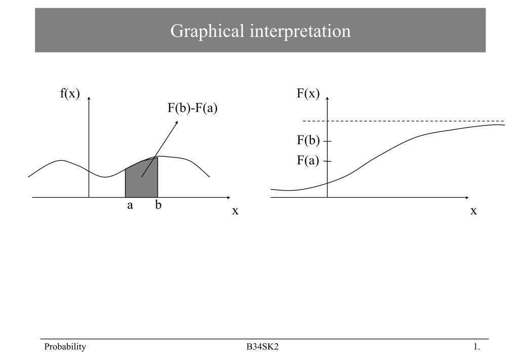
Graphical interpretation

x

f(x)

a b x

F(x)

F(b)F(a)

F(b)-F(a)


Joint distributions

Joint probability function: relates random variables x and y

Independence:

Example: Find: The constant c P(1<X<2,2<Y<3) Are X and Y

independent?


Change of variables

Discrete Variables:

Theorem: Let X be a random variable of probability function f(x) Suppose we have a new random variable U defined as: U = Φ(X) and X = ϕ(U), then the probability function of U is: g(u) = f(ϕ(u)).

Continuous Variables:

Theorem: Let X be a random variable of probability function f(x) Suppose we have a new random variable U defined as:

U = Φ(X) and X = ϕ(U), then the probability function of U is: g(u) = f(ϕ(u)) ϕ’(u)


Sum of random variables

Consider U = X+Y where X and Y are random variables of joint probability density function f(x,y).

The following results hold:

Theorem 1:

Theorem 2: If X and Y are independent we have:


Analysing random variables

Assume now that we have random variables. We want to extract informationfrom these variables in order to analyse and characterise them.

Mathematical expectation: measures central tendancyAlso called expected value, expectation or mean.Definition:

discrete case:

Note: If all probabilities are equal then

ARITHMETIC MEAN!


Expectation

Mathematical expectation:Definition:

continuous case:

Notation: Very often called mean Noted

Example

X of probability density function:

E(X)?


Properties of the expectation

Linearity:1) E(cX) = c E(X)

2) E(X+Y) = E(X)+E(Y)

Other properties:

If X and Y are independent:E(XY) = E(X)E(Y)


Variance and standard deviation

Variance: measures spread around central tendancy

Definition:

Variance: measures spread around central tendancy

Definition:


Properties of Variance

1) var(cX) = c2 E(X)

if X and Y are independent:

2) var(X+Y) = var(X)+var(Y)

3) var(X-Y) = var(X)+var(Y)

Standardized random variable:

Let X be a random variable of mean µ and variance σ, we can define:

which as a null mean and a unity variance.


Covariance for joint distributions

Definition:

Properties:

Correlation Coefficient:


Chebyshev Theorem

This is a major result in probability and statistics.

Chebyshev Theorem:Let X be a random variable with mean µ and variance σ2. Then for any positivenumber ε :

Interpretation?

Remember that we have not even specified the type of distribution!This is a very general result.


Measures of central tendancy

Mode: The mode of a random variable is the value which has the greatest probability of occurring (i.e. the maximum of the probability distribution function). If there are several maxima, the random variable has got several modes.

Median: The median m of a random variable X is the value which separates the probability density function in two halves.

P(X<m) <= 0.5 P(X>m) <= 0.5Graphical interpretation:

Mean ModeMedian


Probability laws. A quick review

Discrete LawsBinomial distributionPoisson distributionGeometric distributionHyperGeometric distribution

Continuous LawsUniform distributionGamma distributionBeta distributionNormal distributionChi-square distributionStudent-t distribution


Stochastic Processes

Definition: A stochastic process is a function of time for which the value of the function at any

time t is a random variable. Several repetitions of the same function will not give the same values but its statistical properties will be preserved.

t

X(t,λ))First realisation

Secondrealisation

Processparameter

Expectation:

Variance


Stochastic Processes

Stationarity A stochastic process is wide sense stationary of order m if and only if its moments of

order up to m are independent of t. A case of particular importance is stationarity of order 2 where:

In this case, the mean is independent of time and the autocorrelation function only depends on time-difference and not absolute time. This enables to study the process on any time interval and to generalise the results at any other time!

Ergodicity So far, we have considered the expectation to measure the characteristics of our

processes. We therefore need lots of realisation of the process to calculate those values. If a process is ergodic, the expectation can be estimated using temporal mean instead. We can therefore derive m and Γ from one realisation of the process!

electronic instrumentation -...

Documents