Electronic InstrumentationExperiment 5

Part A: Bridge Circuit Basics

Part B: Analysis using Thevenin Equivalent

Part C: Potentiometers and Strain Gauges

Agenda

Bridge Circuit • Introduction

• Purpose• Structure• Balance

• Analysis using the Thevenin Equivalent method

Strain Gauge, Cantilever Beam and Oscillations

What you will know:

What a bridge circuit is and how it is used in the experiments.

What a balanced bridge is and how to recognize a circuit that is balanced.

How to apply Thevenin equivalent method to a voltage divider, a Wheatstone Bridge or other simple configuration.

How a strain gauge is used in a bridge circuit

How to determine the damping constant of a damped sinusoid given a plot.

Why use a Bridge?Temperature

Light IntensityPressure

Hydrogen Cyanide Gas

Porter, Tim et al., Embedded Piezoresistive Microcantilever Sensors: Materials for Sensing Hydrogen Cyanide Gas,

http://www.mrs.org/s_mrs/bin.asp?CID=6455&DID=176389&DOC=FILE.PDF .

Strain

Sensors that quantifychanges in physical variables by measuringchanges in resistance ina circuit.

Wheatstone Bridge StructureA bridge is just two voltage dividers in parallel. The output is the difference between the two dividers.

BAoutSBSA VVdVVVRR

RVV

RR

RV

41

4

32

3

A Balanced Bridge Circuit

02

1

2

1

111

11

11

1

VVVVdV

VKK

KVV

KK

KV

rightleft

rightleft

A “zero” point for normal conditions so changes can be positive or negative in reference to this point.

Thevenin Voltage Equivalents In order to better understand how bridges

work, it is useful to understand how to create Thevenin Equivalents of circuits.

Thevenin invented a model called a Thevenin Source for representing a complex circuit using• A single “pseudo” source, Vth

• A single “pseudo” resistance, Rth

RL

0

Vo

0Vdc

R4R2

R1 R3

Vth

FREQ = VAMPL = VOFF =

0

RL

Rth

Thevenin Voltage Equivalents

This model can be used interchangeably with the original (more complex) circuit when doing analysis.

Vth

FREQ = VAMPL = VOFF =

0

RL

Rth

The Thevenin source, “looks” to the load on the circuit like the actual complex combination of resistances and sources.

Thevenin Model

Vs

FREQ = VAMPL = VOFF = RL

Rs

0

Load ResistorRth

Vth

FREQ = VAMPL = VOFF =

0

RL

Any linear circuit connected to a load can be modeled as a Thevenin equivalent voltage source and a Thevenin equivalent impedance.

Note:

We might also see a circuit with no load resistor, like this voltage divider.

R2

0

R1

Vs

FREQ = VAMPL = VOFF =

Thevenin Method

Find Vth (open circuit voltage)• Remove load if there is one so that load is open• Find voltage across the open load

Find Rth (Thevenin resistance)• Set voltage sources to zero (current sources to open) –

in effect, shut off the sources• Find equivalent resistance from A to B

Vth

FREQ = VAMPL = VOFF =

0

RL

Rth

A

B

Example: The Bridge Circuit We can remodel a bridge as a Thevenin

Voltage source

RL

0

Vo

0Vdc

R4R2

R1 R3

Vth

FREQ = VAMPL = VOFF =

0

RL

Rth

Find Vth by removing the Load

Let

Vo=12V

R1=2k

R2=4k

R3=3k

R4=1k

RL

0

Vo

0Vdc

R4R2

R1 R3

0

Vo

0Vdc

R4R2

R1 R3

A AB B

VB

R 4

R 3 R 4

V o

Step 2: Voltage divider for points A and B

VA

R2

R2 R1

Vo

Step 3: Subtract VB from VA to get Vth

VA 8V VB 3V

Step 1: Redraw and remove load from circuit

VB-VA=Vth Vth=5V

To find Rth First, short out the voltage source (turn it

off) & redraw the circuit for clarity.

0

R4R2

R1 R3

A B R 12 k

R 24 k

R 33 k

R 41 k

BA

Find Rth Find the parallel combinations of R1 & R2 and

R3 & R4.

Then find the series combination of the results.

RR R

R R

k k

k k

kk1 2

1 2

1 2

4 2

4 2

8

61 3 3

.

RR R

R R

k k

k k

kk3 4

3 4

3 4

1 3

1 3

3

40 7 5

.

R th R R k k

1 2 3 44

3

3

42 1.

Redraw Circuit as a Thevenin Source

Then add any load and treat it as a voltage divider.

0

Vth

5V

Rth

2.1k

thLth

LL V

RR

RV

Thevenin Applet (see webpage)

Test your Thevenin skills using this applet from the links for Exp 3

Does this really work?

To confirm that the Thevenin method works, add a load and check the voltage across and current through the load to see that the answers agree whether the original circuit is used or its Thevenin equivalent.

If you know the Thevenin equivalent, the circuit analysis becomes much simpler.

Thevenin Method Example Checking the answer with PSpice

Note the identical voltages across the load.• 7.4 - 3.3 = 4.1 (only two significant digits in Rth)

R3

3kVth

5Vdc

0

7.448V

0V

4.132V

3.310VVo

12VdcRload

10k

R1

2k

12.00V

RL

10kR2

4k

5.000V Rth

2.1k

R4

1k

0

Thevenin’s method is extremely useful and is an important topic. But back to bridge circuits – for a balanced

bridge circuit, the Thevenin equivalent voltage is zero.

An unbalanced bridge is of interest. You can also do this using Thevenin’s method.

Why are we interested in the bridge circuit?

Wheatstone Bridge

•Start with R1=R4=R2=R3

•Vout=0

•If one R changes, even a small amount, Vout ≠0

•It is easy to measure this change.

•Strain gauges look like resistors and the resistance changes with the strain

•The change is very small.

BAoutSBSA VVdVVVRR

RVV

RR

RV

41

4

32

3

Using a parameter sweep to look at bridge circuits.

V1

FREQ = 1kVAMPL = 9VOFF = 0

R1350ohms

R2350ohms

R3350ohms

R4{Rvar}

0

Vleft Vright

PARAMETERS:Rvar = 1k

V-

V+

• PSpice allows you to run simulations with several values for a component.

• In this case we will “sweep” the value of R4 over a range of resistances.

This is the “PARAM” part

Name the variable that will be changed

Parameter Sweep

Set up the values to use.

In this case, simulations will be done for 11 values for Rvar.

Parameter Sweep

All 11 simulations can be displayed

Right click on one trace and select “information” to know which Rvar is shown.

Part B

Strain Gauges The Cantilever Beam Damped Sinusoids

Strain Gauges

•When the length of the traces changes, the resistance changes.

•It is a small change of resistance so we use bridge circuits to measure the change.

•The change of the length is the strain.

•If attached tightly to a surface, the strain of the gauge is equal to the strain of the surface.

•We use the change of resistance to measure the strain of the beam.

Strain Gauge in a Bridge Circuit

Cantilever Beam

The beam has two strain gauges, one on the top of the beam and one on the bottom. The strain is approximately equal and opposite for the two gauges.

In this experiment, we will hook up the strain gauges in a bridge circuit to observe the oscillations of the beam.

Two resistors and two strain gauges on the beam creates a bridge circuit, and then its output goes to a difference amplifier

Strain Gauge-Cantilever Beam Circuit

Modeling Damped Oscillations

v(t) = A sin(ωt)

Time

0s 5ms 10ms 15msV(L1:2)

-400KV

0V

400KV

Modeling Damped Oscillations

v(t) = Be-αt

Modeling Damped Oscillations

v(t) = A sin(ωt) Be-αt = Ce-αtsin(ωt)

Time

0s 5ms 10ms 15msV(L1:2)

-200V

0V

200V

Finding the Damping Constant Choose two maxima at extreme ends of the

decay. (t0,v0)(t1,v1)

Finding the Damping Constant

Assume (t0,v0) is the starting point for the decay.

The amplitude at this point,v0, is C. v(t) = Ce-αtsin(ωt) at (t1,v1):

v1 = v0e-α(t1-t0)sin(π/2) = v0e-α(t1-t0)

Substitute and solve for α: v1 = v0e-α(t1-t0)

Finding the Damping Constant

V0=(7s, 4.6 – 2)=(7, 2.6)

4.6

2

V1=(74s, 2.7 – 2)=(74, 0.7)

2.7

2

V1=V0e-α(t1-t0)

0.7=2.6e-α(74-7)

-α(67)=ln (0.7/2.6)

α=0.0196/s

7 74

Harmonic Oscillators Analysis of Cantilever Beam Frequency

Measurements

Next week

Examples of Harmonic Oscillators Spring-mass combination Violin string Wind instrument Clock pendulum Playground swing LC or RLC circuits Others?

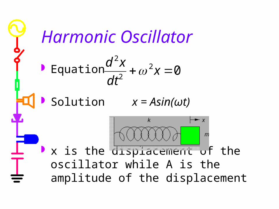
Harmonic Oscillator

Equation

Solution x = Asin(ωt)

x is the displacement of the oscillator while A is the amplitude of the displacement

022

2

xdt

xd

Spring

Spring Force

F = ma = -kx Oscillation Frequency

This expression for frequency holds for a massless spring with a mass at the end, as shown in the diagram.

m

k

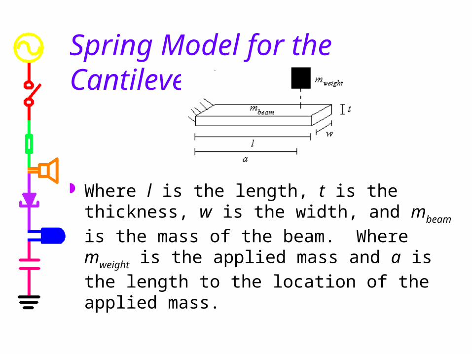
Spring Model for the Cantilever Beam

Where l is the length, t is the thickness, w is the width, and mbeam is the mass of the

beam. Where mweight is the applied mass and

a is the length to the location of the applied mass.

Finding Young’s Modulus For a beam loaded with a mass at the end, a is

equal to l. For this case:

where E is Young’s Modulus of the beam. See experiment handout for details on the

derivation of the above equation. If we can determine the spring constant, k, and we

know the dimensions of our beam, we can calculate E and find out what the beam is made of.

3

3

4l

Ewtk

Finding k using the frequency Now we can apply the expression for the ideal

spring mass frequency to the beam.

The frequency, fn , will change depending upon how much mass, mn , you add to the end of the beam.

2)2( fm

k

2)2( nn

fmm

k

Our Experiment

For our beam, we must deal with the beam mass and any extra load we add to the beam to observe how its performance depends on load conditions.

Real beams have finite mass distributed along the length of the beam. We will model this as an equivalent mass at the end that would produce the same frequency response. This is given by m = 0.23mbeam.

Our Experiment

• To obtain a good measure of k and m, we will make 4 measurements of oscillation, one for just the beam and three others by placing an additional mass at the end of the beam.

20 )2)(( fmk 2

11 )2)(( fmmk 2

22 )2)(( fmmk 233 )2)(( fmmk

Our Experiment Once we obtain values for k and m we can plot

the following function to see how we did.

In order to plot mn vs. fn, we need to obtain a guess for m, mguess, and k, kguess. Then we can use the guesses as constants, choose values for mn (our domain) and plot fn (our range).

nguess

guess

n mm

kf

2

1

Our Experiment

The output plot should look something like this. The blue line is the plot of the function and the points are the results of your four trials.

Our Experiment

How to find final values for k and m.• Solve for kguess and mguess using only two of your

data points and two equations. (The larger loads work best.)

• Plot f as a function of load mass to get a plot similar to the one on the previous slide.

• Change values of k and m until your function and data match.

Our Experiment Can you think of other ways to more

systematically determine kguess and mguess ?

Experimental hint: make sure you keep the center of any mass you add as near to the end of the beam as possible. It can be to the side, but not in front or behind the end.