electrodynamics, problem sets - eth z

Electrodynamics

Problem Sets

ETH/Uni Zurich, FS14

Prof. N. Beisert

c© 2014 ETH Zurich

This document as well as its parts is protected by copyright.Reproduction of any part in any form without prior writtenconsent of ETH Zurich is permissible only for private,scientific and non-commercial use.

Contents

Sheet 1 1.11.1. Vector calculus . . . . . . . . . . . . . . . . . . . . . . . . . . . . . . . . . 1.11.2. Gauß’s theorem . . . . . . . . . . . . . . . . . . . . . . . . . . . . . . . . 1.21.3. Stokes’ theorem . . . . . . . . . . . . . . . . . . . . . . . . . . . . . . . . 1.2

Sheet 2 2.12.1. Potential and electric field strength . . . . . . . . . . . . . . . . . . . . . 2.12.2. Stable equilibrium . . . . . . . . . . . . . . . . . . . . . . . . . . . . . . 2.12.3. Energy stored in a parallel plate capacitor . . . . . . . . . . . . . . . . . 2.12.4. Electric field strength in a hollow sphere . . . . . . . . . . . . . . . . . . . 2.12.5. Delta function . . . . . . . . . . . . . . . . . . . . . . . . . . . . . . . . . 2.2

Sheet 3 3.13.1. Imaginary dipoles . . . . . . . . . . . . . . . . . . . . . . . . . . . . . . . 3.13.2. Conducting sphere in an external electric field . . . . . . . . . . . . . . . 3.13.3. Spherical cavity . . . . . . . . . . . . . . . . . . . . . . . . . . . . . . . . 3.23.4. Capacities . . . . . . . . . . . . . . . . . . . . . . . . . . . . . . . . . . . 3.2

Sheet 4 4.14.1. Spherical multipole moments of a cube . . . . . . . . . . . . . . . . . . . 4.14.2. Current in cylindrical wire . . . . . . . . . . . . . . . . . . . . . . . . . . 4.24.3. Magnetic field of a finite coil . . . . . . . . . . . . . . . . . . . . . . . . . 4.24.4. Rotation gymnastics . . . . . . . . . . . . . . . . . . . . . . . . . . . . . 4.2

Sheet 5 5.15.1. Magnetic moment of a rotating spherical shell . . . . . . . . . . . . . . . 5.15.2. Capacitor filled with dielectric . . . . . . . . . . . . . . . . . . . . . . . . 5.15.3. Iron pipe in a magnetic field . . . . . . . . . . . . . . . . . . . . . . . . . 5.2

Sheet 6 6.16.1. Green’s functions in electrostatics . . . . . . . . . . . . . . . . . . . . . . 6.16.2. Green’s function in two dimensions . . . . . . . . . . . . . . . . . . . . . . 6.26.3. Cartesian multipole expansion . . . . . . . . . . . . . . . . . . . . . . . . 6.36.4. Multipole moments in cartesian and spherical coordinates . . . . . . . . . 6.46.5. Magnetic field in a non-coaxial cylinder cavity . . . . . . . . . . . . . . . 6.46.6. Magnetic field of a circular loop . . . . . . . . . . . . . . . . . . . . . . . 6.46.7. Magnetic field of a kinked wire . . . . . . . . . . . . . . . . . . . . . . . . 6.4

Sheet 7 7.17.1. Charged particle in an electromagnetic field . . . . . . . . . . . . . . . . . 7.17.2. Induction in a magnetic field . . . . . . . . . . . . . . . . . . . . . . . . . 7.17.3. Self-induction of a coaxial cable . . . . . . . . . . . . . . . . . . . . . . . 7.1

Sheet 8 8.18.1. Fourier transform . . . . . . . . . . . . . . . . . . . . . . . . . . . . . . . 8.18.2. Elliptically polarized waves . . . . . . . . . . . . . . . . . . . . . . . . . . 8.18.3. Group velocity . . . . . . . . . . . . . . . . . . . . . . . . . . . . . . . . 8.2

3

Sheet 9 9.19.1. Dynamics of an electric circuit . . . . . . . . . . . . . . . . . . . . . . . . 9.19.2. The Poynting vector . . . . . . . . . . . . . . . . . . . . . . . . . . . . . 9.2

Sheet 10 10.110.1. Feynman’s paradox . . . . . . . . . . . . . . . . . . . . . . . . . . . . . 10.110.2. Plane waves in a conductive medium . . . . . . . . . . . . . . . . . . . . 10.2

Sheet 11 11.111.1. Rectangular waveguide . . . . . . . . . . . . . . . . . . . . . . . . . . . . 11.111.2. Dipole radiation . . . . . . . . . . . . . . . . . . . . . . . . . . . . . . . 11.2

Sheet 12 12.112.1. Optics via the principle of least action . . . . . . . . . . . . . . . . . . . 12.112.2. Refraction of planar waves . . . . . . . . . . . . . . . . . . . . . . . . . 12.212.3. Scattering of light . . . . . . . . . . . . . . . . . . . . . . . . . . . . . . 12.2

Sheet 13 13.113.1. Diffraction through a rectangular slit . . . . . . . . . . . . . . . . . . . . 13.113.2. Invariant distance . . . . . . . . . . . . . . . . . . . . . . . . . . . . . . 13.113.3. Electromagnetic field tensor . . . . . . . . . . . . . . . . . . . . . . . . . 13.213.4. Lienard–Wiechert potential . . . . . . . . . . . . . . . . . . . . . . . . . 13.2

4

Electrodynamics Problem Set 1ETH/Uni Zurich, FS14 Prof. N. Beisert

1.1. Vector calculus

In this problem we recall a number of standard identities of vector calculus which we willfrequently use in electrodynamics.

Definitions/conventions: We commonly write the well-known vectorial differentiation op-

erators grad, div, rot using the vector ~∇ of partial derivatives ∇i := ∂/∂xi as

gradF := ~∇F , div ~A := ~∇· ~A , rot ~A := ~∇× ~A . (1.1)

The components of a three-dimensional vector product ~a ×~b are given by

(~a ×~b)i =3∑

j,k=1

εijkajbk . (1.2)

Here, εijk is the totally anti-symmetric tensor in R3 with ε123 = +1.

a) Show that

3∑i=1

εijkεilm = δjlδkm − δjmδkl and3∑

i,j=1

12εijkεijl = δkl . (1.3)

b) Show the following identities for arbitrary vectors ~a, ~b, ~c, ~d:

~a ·(~b × ~c) = ~b ·(~c × ~a) = ~c ·(~a ×~b) , (1.4)

~a × (~b × ~c) = (~a ·~c)~b − (~a ·~b)~c , (1.5)

(~a ×~b)·(~c × ~d) = (~a ·~c)(~b ·~d)− (~a ·~d)(~b ·~c) . (1.6)

c) Prove the following identities for arbitrary scalar fields F and vector fields ~A, ~B:

~∇× (~∇F ) = 0 , (1.7)

~∇·(~∇× ~A) = 0 , (1.8)

~∇× (~∇× ~A) = ~∇(~∇· ~A)−∆ ~A , (1.9)

~∇·(F ~A) = (~∇F )· ~A + F ~∇· ~A , (1.10)

~∇× (F ~A) = (~∇F )× ~A + F ~∇× ~A , (1.11)

~∇( ~A · ~B) = ( ~A ·~∇) ~B + ( ~B·~∇) ~A + ~A × (~∇× ~B) + ~B × (~∇× ~A) , (1.12)

~∇·( ~A × ~B) = ~B·(~∇× ~A)− ~A ·(~∇× ~B) . (1.13)

−→

1.1

1.2. Gauß’s theorem

Consider the following vector fields ~Ai in two dimensions

~A1 =(3xy(y − x), x2(3y − x)

), (1.14)

~A2 =(x2(3y − x), 3xy(x− y)

), (1.15)

~A3 =(x/(x2 + y2), y/(x2 + y2)

)= ~x

/~x 2 . (1.16)

a) Compute the flux of ~Ai through the boundary of the square Q with corners ~x =(±1,±′1)

Ii =

∮∂Q

dx~n· ~A i . (1.17)

b) Compute the divergence of ~Ai and its integral over the area of this square Q

I ′i =

∫Q

d2x ~∇· ~Ai . (1.18)

1.3. Stokes’ theorem

Consider the vector field~A = (x2y, x3 + 2xy2, xyz) . (1.19)

a) Compute the integral along the circle S around the origin in the xy-plane with radiusR

I =

∮S

d~x · ~A . (1.20)

b) Compute the rotation ~B of the vector field ~A

~B = ~∇× ~A . (1.21)

c) Compute the flux of the rotation ~B through the disk S whose boundary is S, ∂D = S

I ′ =

∫D

d2x~n· ~B . (1.22)

1.2


2.1. Potential and electric field strength

Four point charges are placed at the corners (a, 0), (a, a), (0, a), (0, 0) of a square. Findthe potential and the electric field strength in the plane of this square. Sketch the fieldlines and equipotential lines of the following charge distributions:

a) +q,+q,+q,+q;

b) −q,+q,−q,+q;

c) +q,+q,−q,−q.

Hint: Using Mathematica, the commands ContourPlot and StreamPlot might come inhandy.

2.2. Stable equilibrium

Two balls, each with charge +q, are placed on an isolator plate within the z = 0 planewhere they can move freely without friction. Under the plate, a third ball with charge−2q is fixed at ~r = (0, 0,−b). Treat the balls as point charges, and find stable positionsfor the two balls on the plate.

2.3. Energy stored in a parallel plate capacitor

Two plates with charges +Q and −Q and area A are placed parallelly to each other at a(small) distance d. Find the energy stored in the electric field between them.

2.4. Electric field strength in a hollow sphere

A charged ball with homogeneous charge density ρ and radius RA contains a sphericalcavity with radius RI that is shifted from the centre by the vector ~a with |~a | < RA −RI.Calculate the electric field strength within the cavity.

Hint: Use Gauß’s theorem and the superposition principle to calculate the field strength.

−→

2.1

2.5. Delta function

The delta function is often used to describe point charge densities. It is defined through thefollowing property when integrated over a smooth test function f with compact support∫ ∞

−∞dx f(x) δ(x− a) = f(a) . (2.1)

a) Show that it can be written as the limit limε→0 gε(x) = δ(x) of following function

gε(x) =1√2πε

e−x2/(2ε) . (2.2)

b) Show also that limε→0 hε(x) = δ(x)

hε(x) =1

2πi

(1

x− iε− 1

x+ iε

). (2.3)

c) Show, that the derivative of the delta function satisfies∫ ∞−∞

dx f(x) δ′(x− a) = −f ′(a) . (2.4)

2.2


3.1. Imaginary dipoles

Consider two point charges q and q′ at a distance d from each other, and a plane perpen-dicular to the line through q and q′ in a distance αd from q.

a) Show that, in order for the plane to be at constant potential, one must have q′ = −qand α = 1/2.

Hint : Look at the potential at large distance first.

Now consider a point charge at the (cartesian) coordinates (a, b, 0) in the empty region ofa space filled with a grounded conductor except for positive x and y.

b) Argue that introducing two mirror charges—with respect to the planes x = 0 andy = 0, respectively—is not sufficient to reproduce the boundary conditions of theconductor.

c) Exploiting the symmetry of the problem, introduce one more appropriate virtualcharge and show explicitly that this makes the potential on the planes constant.

Finally, consider a point charge in the empty region of a space filled with a groundedconductor except for the region of the angle 0 ≤ ϕ ≤ π/n (n integer).

d) Determine the distribution of imaginary charges that reproduces the electric field ofthis charge in the empty region of space. What is the value of the electric field on theline where the two faces of the conductor meet?

3.2. Conducting sphere in an external electric field

A conducting sphere, bearing total charge Q, is introduced into a homogeneous electricfield ~E = E~ez. How does the electric field change due to the presence of the sphere? Howis the charge distributed on the surface of the sphere?

Hint : Motivate the following ansatz in spherical coordinates

Φ(r, ϑ, ϕ) = f0(r) + f1(r) cosϑ , (3.1)

and solve the Poisson equation ∆Φ = 0 using the Laplace operator

∆Φ(r, ϑ, ϕ) =1

r2

∂

∂r

(r2∂Φ

∂r

)+

1

r2 sinϑ

∂

∂ϑ

(sinϑ

∂Φ

∂ϑ

)+

1

r2 sin2 ϑ

∂2Φ

∂ϕ2. (3.2)

A set of boundary conditions that completely fixes the solution is:

• at distances far from the sphere, only the homogeneous field shall remain;

• the surface of the conducting sphere has to be an equipotential surface;

• the electric field has to satisfy Gauß’ theorem.

−→

3.1

3.3. Spherical cavity

Consider a spherical cavity with radius R and let the potential on its boundary be specifiedby an arbitrary function U(ϑ, ϕ).

a) Show that one can write the potential as

Φ(~x) =

∫R(R2 − r2)U(ϑ′, ϕ′)

4π(r2 +R2 − 2rR cos γ)3/2sinϑ′ dϑ′ dϕ′, (3.3)

where γ is the angle between ~x and ~x ′. Determine cos γ in terms of the variables ϑ,ϕ, ϑ′ and ϕ′.

Hint: Use the Green function obtained with the method of imaginary charges andre-express vectors therein with spherical coordinates.

b) Write down the most general solution of the Laplace equation in terms of sphericalharmonics Yl,m, then use orthonormality relations to determine the coefficients for thegiven boundary condition.

c) Write down the explicit potential Φ(~x) inside the sphere for the boundary condition

U(ϑ, ϕ) = U0 cosϑ . (3.4)

3.4. Capacities

A simple capacitor consists of two isolated conductors that are oppositely (but equally insize) charged with Q1 = +Q and Q2 = −Q. In general both conductors will have differentelectrical potential and U = Φ1 − Φ2 denotes the potential difference. A characteristicquantity of the capacitor is the capacity C defined by

C =|Q||U |

. (3.5)

Calculate the capacities for the following cases:

a) two big parallel planar surfaces with area A and small distance d;

b) two concentrical, conducting spheres with radii a and b (b > a);

c) two coaxial, conducting cylindrical surfaces of length L and radii a, b (L b > a).

3.2


4.1. Spherical multipole moments of a cube

Positive and negative point charges ±q are located on the corners of a cube with sidelength a. Charges on neighboring corners have opposite signs. The point of origin is thecenter of the cube, and the edges are aligned with the x, y, z-axes. Let the charge atx, y, z > 0 be positive.

a) Determine the positions of the charges in cartesian and spherical coordinates.

b) Determine the charge density in cartesian coordinates and, thereafter, in sphericalcoordinates, using

δ3(~x− ~x0) =1

r2 sinϑδ(r − r0) δ(ϑ− ϑ0) δ(ϕ− ϕ0) , (4.1)

as well as sinϑ = sin(π − ϑ) and cos (π − ϑ) = − cosϑ.

c) Calculate the spherical dipole, quadrupole and octupole moments of this charge con-figuration, using

ql,m =

∫d3r ρ(~r ) rl Y ∗l,m(ϑ, ϕ) , m = −l,−(l − 1), . . . ,+(l − 1),+l . (4.2)

The required spherical harmonics are:

Y00 = 1, Y11 = −√

3

2sinϑ eiϕ,

Y10 =√

3 cosϑ, Y22 =

√15

8sin2 ϑ e2iϕ,

Y21 = −√

15

2cosϑ sinϑ eiϕ, Y20 =

√5

4

(3 cos2 ϑ− 1

),

Y33 = −√

35

16sin3 ϑ e3iϕ, Y32 =

√105

8cosϑ sin2 ϑ e2iϕ,

Y31 = −√

21

16

(5 cos2 ϑ− 1

)sinϑ eiϕ, Y30 =

√7

4

(5 cos3 ϑ− 3 cosϑ

). (4.3)

Further: Yl,−m = (−1)m Y ∗l,m, and thus ql,−m = (−1)m q∗l,m.

−→

4.1

4.2. Current in cylindrical wire

Consider a straight cylindric wire of radius R oriented along the z-axis. The magnitudeof the current density inside this wire depends on the distance from the center of the wireas follows:

j(ρ) = j0e−ρ2/R2

θ(R− ρ) , (4.4)

where ρ =√x2 + y2 and θ(x) is the unit step function.

a) Find the total current I flowing through the wire. Express j0 through I.

b) Find the magnetic field inside and outside the wire as a function of the total current.Sketch the field lines, paying attention to the direction. Let the current flow into thepositive z-direction.

4.3. Magnetic field of a finite coil

Consider a wire coiled up cylindrically along the z-axis. Let R be the radius of thiscylindric coil and L its length (it starts at z = −L/2 and ends at z = +L/2). Letn = N/L be the winding number per unit length and I the (constant) current flowingthrough the wire. You may neglect boundary effects.

Calculate the z-component of the magnetic flux density B for points on the symmetryaxis. Determine the magnetic field for L→∞ at constant n.

4.4. Rotation gymnastics

The rotation group (in N dimensions) is defined starting from the set of linear mappingsof a vector space which leave the canonical scalar product invariant.

a) Prove that a linear transformation which leaves the norm of all vectors invariant alsoconserves the scalar product between two arbitrary vectors. Then show that anymatrix preserving the norm of all vectors is orthogonal.

b) Show that the determinant of any orthogonal matrix is either +1 or −1.

Orthogonal matrices with negative determinant represent transformations that involvereflection. Since we are interested in rotations, let us restrict ourselves to the group ofmatrices with positive determinant, i.e. the special orthogonal group SO(N).

c) Write down the matrices that represent rotations of an infinitesimal angle dϕ aroundthe i-th axis in three dimensions and subtract the identity from each of them. Finda simple expression of the resulting matrices in terms of the totally antisymmetrictensor εijk.

d) Show that infinitesimal rotations commute with each other up to higher order terms,whereas macroscopic rotations do not commute in general.

e) Write down the infinitesimal rotation of angle dϕ around a generic unit vector ~n (usethe fact that ~n is left unchanged). By performing a large number of such rotations,extend the result to macroscopic angles ϕ around ~n. Show that for every rotationwith ϕ ∈ (0, 2π) and arbitrary ~n, there exists another representation with differentϕ′, ~n′.

4.2


5.1. Magnetic moment of a rotating spherical shell

A spherical shell of radius R and charge Q (homogeneously distributed on the surface) isrotating around its z-axis with angular velocity ~ω = ω~ez.

a) Calculate the current density ~j(~r ) = ~v(~r )ρ(~r ).

b) Calculate the magnetic moment ~m = 12

∫d3r(~r ×~j(~r )) of the spherical shell.

c) Show that the leading behaviour of the magnetic field generated by this sphere for

|~r | R is that of a magnetic dipole, and write down the leading term of ~B.

Hint : Use Biot–Savart law and keep only the leading non-vanishing terms in R/|~r |.

d) Now let ~r2 be a vector such that ~r2 ⊥ ~ω and |~r2| R. Calculate the lowest ordercontribution of the force exerted by the magnetic field from the previous part onanother identical sphere placed at a point ~r2 and rotating with angular velocity ~ω2

parallel to ~ω. Due to the large distance between the spheres you can approximatethem as two point-like objects carrying some magnetic moment.

5.2. Capacitor filled with dielectric

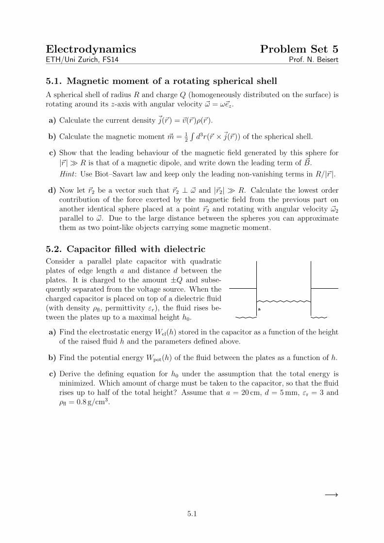
Consider a parallel plate capacitor with quadraticplates of edge length a and distance d between theplates. It is charged to the amount ±Q and subse-quently separated from the voltage source. When thecharged capacitor is placed on top of a dielectric fluid(with density ρfl, permittivity εr), the fluid rises be-tween the plates up to a maximal height h0.

a) Find the electrostatic energy Wel(h) stored in the capacitor as a function of the heightof the raised fluid h and the parameters defined above.

b) Find the potential energy Wpot(h) of the fluid between the plates as a function of h.

c) Derive the defining equation for h0 under the assumption that the total energy isminimized. Which amount of charge must be taken to the capacitor, so that the fluidrises up to half of the total height? Assume that a = 20 cm, d = 5 mm, εr = 3 andρfl = 0.8 g/cm3.

−→

5.1

5.3. Iron pipe in a magnetic field

An infinitely long hollow cylinder (inner radius b, outer radius a) is placed with its axis

orthogonally to the initially homogeneous magnetic field ~B0. The hollow cylinder is madeof iron (permeability µ). The initial field ~B0 can be assumed to be sufficiently small notto saturate the iron, and the permeability µ is constant in the region of interest.

a) Derive the expression for ~B in the cavity (r < b).

Hint : Use the absence of free currents to describe the magnetic field ~H by means ofa scalar potential Φ via ~H = −~∇Φ. The Laplace equation holds in all three relevantregions of space. In cylindrical coordinates (r, ϕ) the Laplacian reads

∆ =1

r

∂

∂r

(r∂

∂r

)+

1

r2

∂2

∂ϕ2+

∂2

∂z2. (5.1)

The boundary conditions of ~H and ~B at the surfaces as well as the behaviour for|~r | → 0 and |~r | → ∞ fix the constants in the solution of the differential equation.

b) Sketch the magnetic field lines in the full region of space, before and after the cylinderhas been placed in the field. Consider also the cases of a paramagnetic (µr > 1), adiamagnetic (µr < 1), and a superconducting (µr = 0) cylinder.

5.2

Electrodynamics Problem Set 6 (Repetition)ETH/Uni Zurich, FS14 Prof. N. Beisert

6.1. Green’s functions in electrostatics

In this problem we analyse the electrostatic Green’s function in more detail. We considerGreen’s functions on a volume V with Dirichlet and Neumann boundary conditions onthe surface ∂V .

a) Apply Green’s second identity,∫V

d3x(φ~∇2ψ − ψ~∇2φ

)=

∮∂V

d2x~n·(φ~∇ψ − ψ~∇φ

)(6.1)

with φ = G(~y, ~x) and ψ = G(~z, ~x). Use that ~∇2xG(~y, ~x) = −δ(3)(~x− ~y ). Express the

difference G(~y, ~z )−G(~z, ~y ) in terms of an integral over the surface ∂V .

b) Show that a Green’s function GD(~x, ~y ) with Dirichlet boundary conditions GD(~x, ~y ) =0 for ~y ∈ ∂V must be symmetric in ~x and ~y.

c) Argue that ~ny·~∇yGD(~x, ~y ) → −δ2(~x − ~y ) for ~x → ∂V and ~y ∈ ∂V . For the case~x 6→ ~y you can use the Dirichlet boundary condition for GD(~x, ~y ). To understand thespecial case ~x→ ~y, integrate the above expression over all ~y ∈ ∂V before performingthe limit.

d) Consider the Neumann boundary condition ~ny·~∇yGN(~x, ~y ) = −F (~y ) for ~y in ∂Vwith

∮∂Vd2xF (~x) = 1. Show that GN(~x, ~y ) is not symmetric in ~x and ~y in general.

Construct a Green’s function G′N(~x, ~y ) = GN(~x, ~y ) +H(~y ) +K(~x) that is symmetricin ~x and ~y. What properties must H and K have?

−→

6.1

6.2. Green’s function in two dimensions

a) In this problem we consider Green’s functions in two dimensions. Consider a Green’sfunction inside the square 0 ≤ x ≤ 1, 0 ≤ y ≤ 1 with Dirichlet boundary conditions onthe edges of the square. Show that the Green’s function which satisfies the boundaryconditions has the expansion

G(x, y, x′, y′) = 2∞∑n=1

gn(y, y′) sin(nπx) sin(nπx′) . (6.2)

The coefficients gn(y, y′) satisfy the conditions(∂2

∂y2− n2π2

)gn(y, y′) = −δ(y′ − y) , (6.3)

gn(y, 0) = gn(y, 1) = 0 . (6.4)

Use the identity for 0 ≤ x, x′ ≤ 1

∞∑n=1

sin(nπx) sin(nπx′) = 12δ(x− x′) . (6.5)

b) The homogeneous solution of the differential equation for gn can be expressed interms of a linear combination of sinh(nπy′) and cosh(nπy′). Make an ansatz in thetwo regions y < y′ und y > y′ that satisfies the boundary conditions and takes intoaccount the discontinuity of the first derivative at y = y′ induced by the source deltafunction. Show that the explicit form of gn is

gn(x, y, x′, y′) =sinh(nπy<) sinh(nπ(1− y>))

πn sinh(nπ), (6.6)

where y< (y>) is the smaller (larger) value of y and y′.

c) Let the square now have a uniform charge density ρ. Furthermore assume that theedges bounding the square are grounded. Use the Green’s function determined aboveto show that the potential is

Φ(x, y) =4ρ

π3ε0

∞∑m=0

sin((2m+ 1)πx)

(2m+ 1)3

·(

1− sinh((2m+ 1)π(1− y)) + sinh((2m+ 1)πy)

sinh((2m+ 1)π)

). (6.7)

−→

6.2

6.3. Cartesian multipole expansion

In this exercise we review the concept of cartesian multipole expansion, which is used todecompose the integral expression of the potentials φ(~x) and ~A(~x), as well as the fields~E(~x) and ~B(~x) created by localised static charge and current densities ρ(~y ) and ~j(~y )into several components. These components have important physical meanings and areof different relevance in the regime of ~x being far away from the source.

We assume that the sources of the electric/magnetic field are contained in an area A ofextension a around the origin. The corresponding scalar potential Φ generated by a givencharge density ρ(~y ) can be written as

Φ(~x) =

∫d3y ρ(~y )

1

4πε0|~x− ~y |. (6.8)

One expects that in the region |~x| a the scalar potential essentially looks like thepotential created by a point charge placed somewhere in A carrying the charge q =∫d3yρ(~y). We will reproduce this behaviour by expanding the term 1/|~x− ~y| for fixed ~x

in a Taylor series of ~x around the point ~y = 0. In the limit |~x| → ∞ this choice of ~y willdrop out, however for finite ~x this choice matters.

a) Calculate the Taylor expansion of 1/|~x− ~y| up to O(1/|~x|4), and use the result toexpand the electric potential of a charge distribution as

Φ(~x) =1

4πε0|~x |

[Q+

xi|~x|2

Qi +xixj2|~x |4

Qij +xixjxk6|~x |6

Qijk

]+O

(1/|~x |5

). (6.9)

Determine the total charge Q, the dipole moment Qi, the quadrupole moment Qij

and the octupole moment Qijk.

b) Now we consider a concrete charge distribution ρ that is generated by a finite dipoleconsisting of a charge +λq at (0, 0, 1/(2λ)) and a charge −λq at (0, 0,−1/(2λ)). Cal-culate Q, Qi, Qij and Qijk. Show that only in the limit λ→∞, we obtain a perfectdipole (i.e. that all other moments of the multipole expansion vanish).

c) The cartesian components Ai of the vector potential can be calculated in the sameway as the scalar potential, i.e.

Ai(~x) = µ0

∫d3y ji(~y )

1

4π|~x− ~y |. (6.10)

Show that the first term in the multipole expansion vanishes in case of a time inde-pendent current density, and calculate the vector potential up to the first order.

−→

6.3

6.4. Multipole moments in cartesian and spherical coordinates

In this problem we will analyse the relation between cartesian and spherical quadrupolemoments. Consider the cartesian quadrupole moment

Qij = Qji =

∫d3x ρ(~x) (3xixj − δij~x 2) , (6.11)

and the spherical quadrupole moments

qlm =

∫dr dϑ dϕ sinϑ ρ(~x) r2+l Y ∗l,m(ϑ, ϕ) . (6.12)

Express the cartesian multipole moments Qij through the spherical ones for l = 2 and usethe following identities,

Y2,±2(ϑ, ϕ) =

√15

8sin2 ϑ e±2iϕ ,

Y2,±1(ϑ, ϕ) = ∓√

15

2cosϑ sinϑ e±iϕ ,

Y2,0(ϑ, ϕ) =

√5

4

(3 cos2 ϑ− 1

). (6.13)

6.5. Magnetic field in a non-coaxial cylinder cavity

Consider a conducting cylinder of radius a, with a cylindrical cavity of radius b whoseaxis is parallel to the axis of the conducting cylinder. The distance between the axes isd, and d + b < a. The current density ~j is uniform through the conductiong part of thecylinder. Calculate the magnetic field ~B inside the cavity.

Hint : Use the superposition principle and Ampere’s law,∮∂S

~B·d~r = µ0

∫S

d2x~n·~j . (6.14)

6.6. Magnetic field of a circular loop

Consider a conducting wire forming a circle of radius R in the centre of the x-y-plane. Aconstant current I flows counterclockwise through this loop.

a) Calculate the magnetic field ~B at some point on the z-axis.

b) Now calculate the magnetic field ~B at an arbitrary point in the x-y-plane.

6.7. Magnetic field of a kinked wire

An infinite wire carrying a constant current I runs along the positive y-axis, kinks at theorigin, and then runs along the positive x-axis. Show that the magnetic field ~B in thex-y-plane for x, y > 0 is given by

~B =µ0I

4π

(1

x+

1

y+

x

y√x2 + y2

+y

x√x2 + y2

)~ez . (6.15)

6.4


7.1. Charged particle in an electromagnetic field

Consider a point particle carrying charge q in an electromagnetic field, described by avector potential ~A and a scalar potential Φ. The Lagrangian of the particle is given by

L(~x, ~x, t) = 12m~x2 + q~x· ~A(~x, t)− qΦ(~x, t) , (7.1)

where ~x is the position of the particle and m is its mass.

a) Determine the canonical momentum ~p ,

~p =∂L(~x, ~x, t)

∂~x. (7.2)

What is the relation between the canonical momentum ~p and the kinetic momentumm~x? Perform a Legendre transformation to determine the Hamiltonian,

H(~x, ~p , t) = ~p ·~x− L(~x, ~x, t) . (7.3)

b) Use ~B = ~∇× ~A to explicitly verify

3∑j=1

(∂Aj∂xi− ∂Ai∂xj

)xj =

(~x× ~B

)i. (7.4)

c) Start from the Hamiltonian equations

pi = −∂H∂xi

, xi =∂H

∂pi(7.5)

and derive the equation of motion for the charged particle in an electromagnetic field

m~x = q(~E + ~x× ~B

). (7.6)

7.2. Induction in a magnetic field

A homogeneous magnetic field ~B is aligned along the z-axis. Within this magnetic field, aconducting wire forming a circle of radius R rotates with circular velocity ~ω. Its rotationalaxis lies in the plane of the conductor and passes through its centre. Let ϕ be the anglebetween the rotational axis and the field direction. Find the induced voltage in theconductor as a function of time.

7.3. Self-induction of a coaxial cable

A coaxial cable is represented by two coaxial conducting cylindrical shells with radii R1

and R2 with R1 < R2. A current I is flowing through each of the cylindrical shellsalong their axes in opposite directions. Calculate the self-induction per unit length of thiscoaxial cable.

Hint: First calculate the magnetic field of the cable. Then determine its self-inductionfrom the magnetic energy of the cable via

Wm = 12LI2 . (7.7)

7.1


8.1. Fourier transform

The Fourier transformation and its inverse are given by

f(~x) =

∫d3k

(2π)3f(~k) ei

~k·~x , f(~k) =

∫d3x f(~x) e−i

~k·~x . (8.1)

Calculate the Fourier transform of the following functions/equations. The functions fand g have Fourier transforms f and g.

a) af(~x) + bg(~x) (a, b ∈ C),

b) ~∇f(~x),

c) f(~x) g(~x),

d) f(~x) = f ∗(~x),

e) δ3(~x),

f) ~∇δ3(~x).

8.2. Elliptically polarized waves

A wave ~E(~x, t) with the wave vector ~k = k~ez is given by

Ex(~x, t) = A cos(kz − ωt) ,Ey(~x, t) = B cos(kz − ωt+ ϕ) . (8.2)

a) The path of the vector ~E(0, t) describes the polarization of the wave. Show that it isan ellipse. For which values of A, B and ϕ is it a circle?

Hint : The equation of an ellipse is given by

aE2x + 2bExEy + cE2

y + f = 0 , (8.3)

where b2 − ac > 0 and f < 0 .

b) Show that for general A and B the wave could be written as a superposition of twoopposite circularly polarized waves,

~E(~x, t) = ~E+(z, t) + ~E−(z, t) , (8.4)

where E±(z, t) = Re(A±~e±ei(kz−ωt)). A± is a constant and ~e± = 1√

2(~ex + i~ey). Deter-

mine A± as a function of A, B, and ϕ.

Hint: Write the wave as the real part of a complex vector and express ~ex and ~ey asfunctions of ~e±.

−→

8.1

8.3. Group velocity

A Gaussian wave packet φ(x, t) is moving in a dispersive medium (i.e. ω(k) dependsnon-linearly on k). At time t = 0 it is given by

φ(x, t = 0) = exp

(− x2

2(∆x)2

), (8.5)

where we consider ∆x as a measure for the spatial extent of the wave packet. The timedependency is given by

φ(x, t) = Re

∫ ∞−∞

dk

2πφ(k) eikx−iω(k)t , (8.6)

where φ(k) is the Fourier transform of φ(x, t = 0) .

a) Show by completing the squares that the Fourier transform wave packet at t = 0 hasa Gaussian profile. What is the relation between ∆x and the analogous ∆k? Whatdoes this mean?

Hint : ∫ ∞−∞

dx exp

(−(x− µ)2

2σ2

)=√

2π |σ| . (8.7)

b) Show that the maximum of the wave packet covers a distance of vgt in the timeinterval t, where the group velocity vg is given by

vg =dω

dk

∣∣∣∣k0

. (8.8)

Here, k0 denotes the wave number at the maximum of φ(k).

Hint: Expand ω(k) to the first order in k around k0, and evaluate the change in themaximum of the wave packet using (8.6).

c) What is the speed of the individual phase? Under which circumstances do phasevelocity and group velocity of the wave coincide?

d) Estimate how fast the wave packet is widening by finding an expression for the varia-tion of the group velocity inside the pulse. Use the relation between ∆k and ∆x frompart a), and interpret the result accordingly.

Hint: Estimate the variation as the difference between the group velocities at k0 andk0 +∆k (analoguously to (8.8)), and determine ∆vg from an expansion of ω(k) aroundk0 up to the first contributing order.

8.2


9.1. Dynamics of an electric circuit

Consider the circuit shown in (9.1). The circuit consists of a voltage source ξ, a resistorof resistance R, a capacitor of capacitance C, and a solenoid of inductance L.

Note: The laws for the three devices are: U = RI, Q = CU , U = LI, respectively.

2

1

RC

L

(9.1)

a) When the switch is in position 1, the voltage source, resistor and capacitor forma circuit. Assume that capacitor is initially uncharged. For the switch in position1, write down a differential equation for the charge on the capacitor, solve it, andcalculate the time it takes the capacitor to charge to (1−1/e) of its maximal capacity.

When the switch is in position 2, the solenoid, resistor and capacitor form a circuit.Assume that the capacitor is fully charged when the switch is set to position 2 (timet = 0). Correspondingly, there are no currents flowing in the circuit at time t = 0.

b) For the switch in position 2, write down a differential equation for the charge on thecapacitor in the case R = 0, solve it, and find the natural frequency of the the circuit.

c) Now set R > 0. Write down the corresponding differential equation, solve it, andsketch the charge on the capacitor as a function of time. Discuss the three differentcases that can arise.

−→

9.1

9.2. The Poynting vector

Maxwell’s equations in vacuum are given by

~∇× ~E = − ~B , ~∇× ~B = µ0~j + ε0µ0

~E , (9.2)

and the speed of light is c = 1/√ε0µ0.

a) Proove the following identity,

1

2

∂

∂t

(c2 ~B 2 + ~E 2

)= −c2~∇·

(~E × ~B

)− 1

ε0

~E·~j . (9.3)

b) Consider a particle with charge q moving in the electromagnetic field with velocity ~v.Show that the derivative of its kinetic energy is given by

Wkin = q~v· ~E . (9.4)

What is the equivalent for a continuous charge distribution?

The Poynting vector is defined as

~S = ε0c2 ~E × ~B . (9.5)

c) Prove Poynting’s theorem,

∂

∂t

(12ε0

∫V

d3x(c2 ~B 2 + ~E 2

)+Wkin

)= −

∫∂V

d2x~n·~S , (9.6)

where V is some volume and ∂V its surface. For Wkin, insert your result from b).Interpret the physical meaning of each of the terms.

d) Show that the time-averaged Poynting vector for a plane wave in a non-conductingmedium can be written as

〈~S 〉 = 12ε0c

2 Re(~E0 × ~B∗0

), (9.7)

where ~E0 and ~B0 are the (complex) amplitudes of the electric and magnetic fieldswith the time dependency eiωt,

~E(t) = Re( ~E0eiωt) , ~B(t) = Re( ~B0e

iωt) . (9.8)

Hint: Compute the average value over a period T ,

〈~S〉 =1

T

∫ T

0

~S(t) dt . (9.9)

9.2


10.1. Feynman’s paradox

R

B

(10.1)

Consider a long straight wire along the z-axis carrying a uniform linear charge density λ,surrounded by an equally long cylindrical shell of nonconducting material which bears auniform surface charge density σ. Let the radius of the shell be R, and let the values of σand λ be chosen in such a way that the net electric charge per unit length of the systemvanishes. Moreover, a conducting wire (covered with an insulator) is coiled around thecylindrical shell with number of turns per length n. The shell is free to rotate withoutfriction around the symmetry axis and has a mass per unit length equal to ρ, includingthe wire.

The system is initially at rest, with a current i0 flowing through the solenoid. The currentinside the coil is then decreased until it vanishes, e.g. because it is powered by a batteryat the end of its lifetime.

a) Compute the torque d ~M exerted on a slice of the cylindrical shell of height dz by thenon-conservative electric field due to the changing current.

b) Compute the magnetic field generated by a cylindrical shell with surface charge den-sity σ that rotates with angular speed ω around its symmetry axis.

c) Compute the final angular frequency ωf of the system by integrating the torque overtime. Account for the final flux of magnetic field due to the motion of charges.

The considered situation seems to lead to a paradox: there are no external torques actingon the cylindrical shell, yet the angular momentum appears to change from being zeroto some finite value during the experiment. The second part of the exercise is meant toresolve this apparent contradiction.

d) Find the Poynting vector ~S everywhere for a generic static, constant magnetic field~B along the z-axis inside the cylinder; then use it to compute the angular momentumassociated with the electromagnetic field configuration.

e) Write down the appropriate angular momentum conservation law and use it to cross-check your result for ωf . Explain why the argument that led to inconsistency doesnot hold.

−→

10.1

10.2. Plane waves in a conductive medium

a) We consider plane waves in free space. Derive the wave equations for the electromag-netic field from the Maxwell equations. Show that the plane wave,

~E(~x, t)~B(~x, t)

= Re

[~E0

~B0

exp(i~k·~x− iωt

)], (10.2)

represents a solution of these equations and derive the dispersion relation. What isthe wave velocity?

b) Now consider a medium with finite conductivity σ > 0. Here the current density

and the electric field are connected by ~j = σ ~E. Find the wave equation for theelectromagnetic field in this case and show that the amplitude of a plane wave decayswith the penetration depth into the medium.

c) For a low-frequency wave, calculate the penetration depth δ characterising the depthto which a plane wave can enter a conductive medium. δ is conventionally defined asthe distance at which the amplitude of the plane wave decays by a factor e.

10.2


11.1. Rectangular waveguide

Consider an waveguide extended infinitely along the z-axis with a rectangular basis 0 <x < dx and 0 < y < dy. Its surfaces are ideal conductors. Due to the geometry of theproblem, you can make the following ansatz for propagating electromagnetic waves,

~E(x, y, z, t) = Re(~E0(x, y) ei(kz−ωt)

),

~B(x, y, z, t) = Re(~B0(x, y) ei(kz−ωt)

). (11.1)

a) The 3D-vectors split into 2D-vectors (here: x- and y-components) and scalars (z-component). From the Maxwell equations, derive equations for the x- and y-compo-

nents of ~E0 and ~B0 in terms of their z-components, and show the following equationsto hold for the z-components,[

∂2

∂x2+

∂2

∂y2+(ωc

)2

− k2

]Ez = 0 ,[

∂2

∂x2+

∂2

∂y2+(ωc

)2

− k2

]Bz = 0 . (11.2)

b) Express the boundary conditions E‖ = B⊥ = 0 as conditions for the z-components ofthe fields.

c) Determine the solutions for so-called transverse magnetic waves (TM waves), whichsatisfy Bz = 0.

d) Show that no transverse electromagnetic (TEM) waves (i.e. waves with Ez = Bz = 0)exist in an ideal waveguide.

Hint: Use Gauss’ theorem and Faraday’s law as well as the boundary condition forE‖ to show that there are no TEM waves in this waveguide.

−→

11.1

11.2. Dipole radiation

A thin, ideal conductor connects two metal balls at positions z = ±a. The charge densityis

ρ(~x, t) = Qδ(x)δ(y)[δ(z − a)− δ(z + a)

]cos(ωt) (11.3)

with a, Q and ω constant. The current between the two metal balls flows along the wire.

a) Calculate the time average of the angular distribution of the radiation power 〈dP/dΩ〉.Hint: Calculate first the vector potential ~A(~x, t) from the current density ~j and usesimplifying approximations.

b) Calculate 〈dP/dΩ〉 in dipole approximation using the formula⟨dP

dΩ

⟩=⟨|~p|2⟩ sin2 ϑ

16π2ε0c3. (11.4)

11.2


12.1. Optics via the principle of least action

Fermat’s principle states that light travelling between two points in space ~x1 and ~x2 shouldminimise the optical path. The latter is given by

S =

∫ ~x2

~x1

n(~x) dl, (12.1)

where n(~x) denotes the refractive index of the matter and dl =√dx2 + dy2 + dz2 is the

length of the infinitesimal element of the trajectory connecting ~x1 to ~x2. This can bedirectly interpreted as the principle of least action.

Hint: It is convenient to parametrise the trajectory for this integral, namely

S =

∫ t2

t1

n(~x(t))dl

dtdt =

∫ t2

t1

n(~x(t))

√(∂x

∂t

)2

+

(∂y

∂t

)2

+

(∂z

∂t

)2

dt . (12.2)

a) Find the trajectory of light between two points in a homogeneous medium.

(12.3)

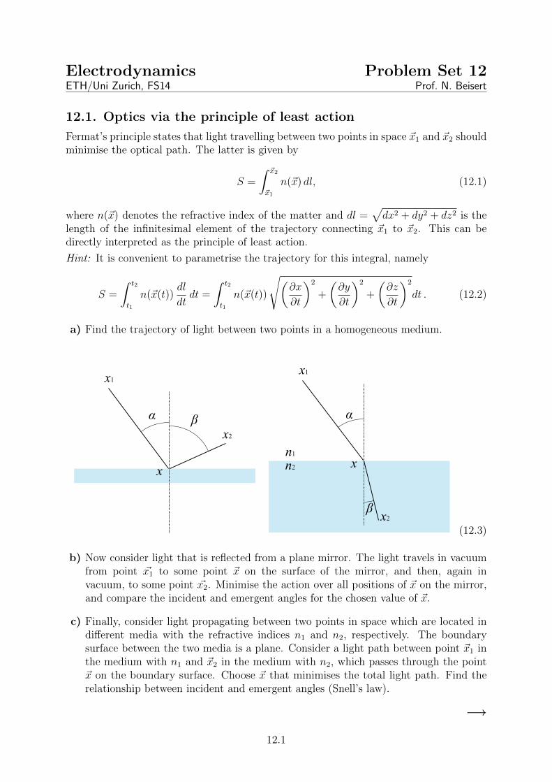
b) Now consider light that is reflected from a plane mirror. The light travels in vacuumfrom point ~x1 to some point ~x on the surface of the mirror, and then, again invacuum, to some point ~x2. Minimise the action over all positions of ~x on the mirror,and compare the incident and emergent angles for the chosen value of ~x.

c) Finally, consider light propagating between two points in space which are located indifferent media with the refractive indices n1 and n2, respectively. The boundarysurface between the two media is a plane. Consider a light path between point ~x1 inthe medium with n1 and ~x2 in the medium with n2, which passes through the point~x on the boundary surface. Choose ~x that minimises the total light path. Find therelationship between incident and emergent angles (Snell’s law).

−→

12.1

12.2. Refraction of planar waves

A planar wave is incident perpendicularly onto a planar layer between two media. Theindices of refraction of the three non-magnetic layers are n1, n2 and n3. The thickness ofthe central layer d, while the other two media each fill half spaces.

a) Calculate the reflection and transmission coefficients (i.e. the ratio of the reflectedand transmitted wave with the incoming energy flux).

Hint: The time-averaged energy-flux density of a complex wave is given by⟨~S⟩

=1

2µ0

Re( ~E × ~B∗) . (12.4)

b) Let the medium with index n1 be part of an optical system (e.g. a lens), and themedium with index n3 be the air (n3 = 1). The surface of the first medium, shouldhave a layer of the medium with index n2 of such a thickness that for a given frequencyω0, there is no reflected wave. Determine the thickness d and the index of refractionn2 of this layer.

12.3. Scattering of light

Classical light-scattering theory (known as a Rayleigh theory) is used to describe lightbeing scattered off small molecules (with an extension much smaller than the wavelength λof the light). Here we consider electric and magnetic fields and intensity of light scatteredoff small particles.

a) First consider a plane monochromatic light wave propagating in x direction, whichis polarised in z-direction. This wave is scattered off a small polarisable, but non-magnetic particle at the origin. The incident wave induces a dipole moment to theparticle, that is proportional to the local field, ~p(t) = α~E(0, t), where α is its polaris-ability. Determine the electric and magnetic fields of the scattered wave at a far-awaypoint ~x, depending on the incident field E0, the distance from the origin r, and theangle ϑ between ~x and the z-axis.

b) Calculate the intensity of this scattered light wave, at a point ~x far away from thescattering particle

Hint: Use the Poynting vector.

c) Use the wave-length dependence of the intensity of the scattered wave (∝ 1/λ4)derived in the previous subproblem, to explain qualitatively the blue colour of thecloudless sky and the red colour of the sunrise and the sunset.

12.2


13.1. Diffraction through a rectangular slit

A rectangular opening with sides of length a and b (b ≥ a) with corners at x = ±a/2,y = ±b/2 is located in a flat, perfectly conducting sheet filling the xy-plane. A planewave propagating in z-direction with linear polarisation at an angle of α w.r.t. the y-axishits the opening.

a) Calculate the diffracted fields and power per unit solid angle with the vectorialSmythe–Kirchhoff relation,

~E(~x) =ieikr

2πr~k ×

∫A

d2x′ ~n× ~E(~x ′) e−i~k·~x ′

, (13.1)

assuming that the tangential electric field in the opening is the unperturbed incidentfield.

b) Calculate the corresponding result with the scalar Kirchhoff approximation.

13.2. Invariant distance

Show that the squared distance s212 = sµ12s12,µ (s12 = x1 − x2) of two spacetime points x1

and x2, is a Lorentz scalar, i.e. s12 = s′12. To do so, use a Lorentz boost with arbitrarydirection and velocity,

t′ = γt− γ

c2~x·~v, ~x ′ = ~x− γ~vt+ (γ − 1)

~x·~v~v 2

~v , (13.2)

with γ = 1/√

1− ~v 2/c2.

a) First, bring the above transformation into a matrix form,

x′µ = (Λ−1)µνxν . (13.3)

b) Now choose ~v = (1, 0, 0)v and show that Λ defines a Lorentz transformation, i.e.

ΛλµηλσΛσν = ηµν . (13.4)

c) Finally, show that the squared distance is Lorentz invariant.

−→

13.1

13.3. Electromagnetic field tensor

The electromagnetic field tensor is defined by

Fµν := −∂µAν + ∂νAµ =

0 1

cEx

1cEy

1cEz

−1cEx 0 −Bz +By

−1cEy +Bz 0 −Bx

−1cEz −By +Bx 0

. (13.5)

a) Show that the electromagnetic field tensor is invariant under the gauge transformation

Aµ → A′µ = Aµ + ∂µχ (13.6)

for any scalar field χ.

b) The dual electromagnetic field tensor is defined by

Fµν := 12εµνρσF

ρσ . (13.7)

Determine the matrix Fµν .

c) Calculate the contractions FµνFµν , FµνF

µν and FµνFµν .

13.4. Lienard–Wiechert potential

Consider a charge moving straight along the positive z-axis with a uniform velocity vstarting at z = 0 at t = 0. Show that its potential is given by

Φ(~x, t) =q

4πε0

1√(z − vt)2 + (1− v2/c2)(x2 + y2)

. (13.8)

13.2

electrodynamics, problem sets - eth z

Documents