electrodynamics of rotating...
TRANSCRIPT
Electrodynamics of Rotating SystemsKirk T. McDonald
Joseph Henry Laboratories, Princeton University, Princeton, NJ 08544(August 6, 2008; updated March 9, 2016)
1 Problem
Discuss methods of analysis of the electrodynamics of rotating systems in the practical limitthat the velocity v of any point in the system with respect to the (inertial) laboratory frameis small compared to the speed of light c.
In particular, discuss whether the magnetic field B′ observed in the frame of the rotatingsystem is that same as the field B observed in the lab frame,
B′ = B, (1)
or whether a better approximation is
B′ = B − v
c× E, (2)
in Gaussian units, where E is the electric field in the lab frame, and v = ω × x is thevelocity in the lab frame of an observer at position x′ = x in the rotating frame, whoseangular velocity with respect to the lab frame is ω.
2 Solution
2.1 Use of Special Relativity
In many examples of electrodynamics of rotating systems we are less interested in the fieldsobserved in the rotating frame than those in the lab frame. Yet, it may be that knowledgeof some aspects of the fields in the moving frame is helpful in reaching an understandingof the fields in the lab frame. In this case, it is often convenient to characterize the fieldsnear some point in the moving frame via the use of Lorentz transformations between thelab frame and the comoving, inertial (nonrotating) frame in which that point in the rotatingsystem is instantaneously at rest. For reviews of this approach, see [1, 2].
If the rotating system includes linear, isotropic media with (relative) permittivity ε and/or(relative) permeability μ that differ from unity, the electrodynamic description should includethe “auxiliary” fields D = E + 4πP and H = B − 4πM, where P and M are the electricand magnetic polarization densities. Solutions to Maxwell’s equations for B, D, E and H interms of the free charge density ρ and the conduction current J can only be obtained usingknowledge of the constitutive equations that relate D and H to E and B. These relations aresimple in an inertial rest frame of the medium,
D = εE, B = μH (inertial rest frame), (3)
1
and in general take more complicated forms in frames in which the medium is in motion,and in non inertial frames even if the medium is at rest there. For example, the constitutiveequations in an inertial frame in which the medium has velocity v with v � c can be written
D = εE+ (εμ− 1)v
c×H, B = μH+ (εμ− 1)
v
c×E,
⎛⎝ medium with velocity v
w.r.t. an inertial frame
⎞⎠ (4)
as first noted by Minkowski [3] (who gave the relations for any v < c).The lab-frame constitutive equations (3) can also be expressed in terms of the polariza-
tions P and M as
P =ε − 1
4πE +
(ε − 1
μ
)v
c× B, M =
(1 − 1
μ
)B
4π+ (εμ − 1)
v
c×E. (5)
In a rotating system with nontrivial electrical media, such as the Wilson-Wilson exper-iment [4, 5], the use of a comoving inertial frame leads us to understand that the rela-tions (4)-(5) are valid in the lab frame in the small region where the medium has velocityv.1
2.2 Electrodynamics in a Rotating Frame
If a description is desired of the electrodynamics of a rotating system according to an observerat rest in that system, the methods of general relativity should be used.
One of the first analyses of electrodynamics in a rotating frame using general relativitywas made by Schiff [6]. See also [7]-[30]. Just as mechanical analyses in rotating framesinclude “fictitious” forces, electrodynamic analysis in rotating frames include “fictitious”charges and currents.2
Sections 2.2.1-2 present a “naive” derivation, due to Modesitt [16], of Schiff’s results[6] for media with ε = 1 = μ. Section 2.2.3 presents a possible alternative description forrotating electrodynamics that appears more compatible with special relativity, but which isfound in sec. 2.2.4 to be in contradiction with a thought experiment at order v/c. Section2.2.5 summarizes a description of the electrodynamics of the nontrivial, rotating electricalmedia. A long Appendix presents a “covariant” discussion of electrodynamics in a rotatingframe when ε and μ differ from unity.
2.2.1 Fields Observed in a Rotating Frame
We desire the fields E′ and B′ seen by an observer in a frame that rotates with angularvelocity ω with respect to the lab frame, where ω = ω z is parallel to the angular velocity ωof the rotating system in the lab frame. We restrict our attention to points x′ in the rotatingframe such that the velocity v = ω × x′ of the points with respect to the lab frame is small
1We shall find in Appendix A.5 that the constitutive equations have a slightly different form than eq. (3)in the rotating frame.
2The adjective “fictitious” is misleading in that to an observer in the rotating frame the “fictitious”forces and charge and current densities appear to be very “real”.
2

compared to the speed of light. Then, we can largely ignore issues of whether rods and clocksin the rotating frame measure the same lengths and time intervals as would similar rods andclocks in the lab frame, and whether the speed of light is the same in both frames. That is,we ignore Ehrenfest’s paradox [31].
We also restrict ourselves to the case that all media have unit (relative) permittivity εand unit (relative) permeability μ.
The (cylindrical) coordinates in the rotating frame are related to those in the lab frameby
r′ = r, φ′ = φ − ωt, z′ = z, t′ = t. (6)
This transformation preserves volume, so conservation of electric charge implies that thetransformation of charge and current density is
ρ′ = ρ, J′ = J − ρv, (7)
where v is the velocity of the observer in the rotating frame with respect to the lab frame.Force F is also invariant under the transformation (6). Thus, a charge q at rest in therotating frame experiences the Lorentz force
F′ = qE′ = F = q(E +
v
c×B
), (8)
and hence the transformation of the electric field is
E′ = E +v
c× B. (9)
The force density on current J in a neutral conductor in the lab frame is J/c × B. For thisto equal the force density J′/c × B′ in the rotating frame, we find, using (7), that
B′ = B, (10)
which clearly holds on the axis of rotation.3
2.2.2 Maxwell’s Equation in a Rotating Frame
According to the transformation (6), intervals of distance, area and volume are measured tobe the same in both frames, so that
∇ = ∇′. (11)
3We shall see in sec. 2.2.2 that the transformations (7) and (9)-(10) lead to Schiff’s forms for Maxwell’sequations in the rotating frame [6]. As remarked in sec. 4 of [32], these transformations do not leave theform of Maxwell’s equations for B and E invariant under a Galilean transformation with v = constant. Ifthe transformations (9)-(10) are supplemented by D′ = D and H′ = H − v/c × D and the transformations(7) are taken to apply to the free charge density and the conduction current, then Maxwell’s equations for Band D, E and H are invariant under a Galilean transformation with velocity v. Using this generalization forthe velocity v of a rotating observer does not, however, lead to the generalization of Schiff’s analysis reportedin [27] as it implies that ∇′ ·D′ = 4πρ′; nor would it lead to an adequate explanation of the Wilson-Wilsonexperiment [4] (where we must find that D = εE + (εμ − 1)v/c×H in the lab frame [5]) by supposing thatthe constitutive equations for a linear, isotropic medium are D′ = εE′ and B′ = μH′ in the rotating frame.
3

Hence, the lab-frame Maxwell equation ∇ · B transforms to
∇′ · B′ = 0, (12)
recalling eq. (10). Similarly, the lab-frame Maxwell equation ∇ · E = 4πρ transforms to
∇′ ·E′ = 4πρ′+∇′ ·(v
c× B′
)= 4πρ′+B′ ·∇′×v
c− v
c·∇′×B′ = 4πρ′+
2ω · B′
c−v
c·∇′×B′,
(13)using eqs. (7)-(10) and recalling that v = ω × x′, so ∇′ × v = 2ω.
More care is required in dealing with transformations of time derivatives to the rotatingframe. We recall that the total lab-frame time derivative of a lab-frame vector field Aaccording to an observer with velocity v in the lab is given by the convective derivative,
dA
dt=
∂A
∂t+ (v · ∇)A. (14)
Similarly, if the observer has velocity v′ in the rotating frame, the total time derivative inthat frame is
dA
dt′=
∂A
∂t′+ (v′ · ∇′)A. (15)
These two total time derivative are related by
dA
dt=
dA
dt′+ ω × A. (16)
For an observer at rest in the rotating frame, v′ = 0 and v = ω × x, so that
dA
dt′=
∂A
∂t′, (17)
and eqs. (14) and (16)-(17) can be combined to give4
∂A
∂t=
∂A
∂t′+ ω × A − (v · ∇)A. (18)
Some useful vector facts are
∇ · v = ∇ · ω × x = −ω · ∇ × x = 0, (19)
ω × A = ω × (A · ∇)x = (A ·∇)ω × x = (A · ∇)v, (20)
and hence,
∇ × (v × A) = v(∇ · A) − A(∇ · v) + (A · ∇)v − (v · ∇)A
= v(∇ · A) + ω × A− (v · ∇)A. (21)
4A subtle issue here is that the vector A that appears in the term ∂A/∂t′ is not the transform oflab-frame vector A to the rotating frame; rather it is still the lab-frame vector A.
4

For later use we note that v = ω × x = ωr φ, where x = (r, φ, z) in cylindrical coordinates,so that
∇× (v ×A) = v(∇ · A) + ω × A − ω∂A
∂φ. (22)
Using eq. (21) in (18), we have
∂A
∂t+ v(∇ · A) =
∂A
∂t′+ ∇ × (v × A). (23)
A special case is that A = v, for which ∂v/∂t′ = 0, so that eqs. (19), (22) and (23) lead to∂v/∂t = ω × v as expected.
Thus, the partial time derivatives of the magnetic field B are related by
∂B
∂t=
∂B
∂t′+ ∇ × (v × B) =
∂B′
∂t′+ ∇′ × (v × B′). (24)
Faraday’s law can now be transformed as
∇ × E = ∇′ ×(E′ − v
c× B′
)= −1
c
∂B
∂t= −1
c
∂B′
∂t′−∇′ ×
(v
c× B′
), (25)
which simplifies to
∇′ × E′ = −1
c
∂B′
∂t′. (26)
The partial time derivative of the electric field E = E′ − v/c × B′, where ∇ · E = 4πρ,is, according to eq. (23),
∂E
∂t+ 4πρ v =
∂E
∂t′+ ∇ × (v × E) =
∂E′
∂t′− v
c× ∂B′
∂t′+ ∇′ ×
[v ×
(E′ − v
c×B′
)]. (27)
Using this, and recalling from eq. (7) that J = J′ + ρ v, the fourth Maxwell equationtransforms as
∇×B = ∇′×B′ =4π
cJ+
1
c
∂E
∂t=
4π
cJ′ +
1
c
∂E′
∂t′− v
c2× ∂B′
∂t′+∇′ ×
[vc×(E′ − v
c× B′
)].
(28)Maxwell’s equations (12)-(13), (26) and (28) in the rotating frame are
∇′ · E′ = 4πρ′ +2ω · B′
c− v
c· ∇′ × B′, (29)
∇′ × E′ = −1
c
∂B′
∂t′, (30)
∇′ · B′ = 0, (31)
∇′ × B′ =4π
cJ′ +
1
c
∂E′
∂t′− v
c2× ∂B′
∂t′+ ∇′ ×
[vc×(E′ − v
c× B′
)], (32)
which are the forms given by Schiff [6].In practical rotating systems terms in v2/c2 are negligible, so eq. (32) simplifies slightly
to
∇′ ×(B′ − v
c×E′
)≈ 4π
cJ′ +
1
c
∂E′
∂t′− v
c2× ∂B′
∂t′. (33)
Using this in eq. (29) we have, to order v/c,
∇′ · E′ ≈ 4π
(ρ′ − v · J′
c2
)+
2ω · B′
c− v
c2· ∂E′
∂t′. (34)
5
2.2.3 Another Description of Electrodynamics in the Rotating Frame
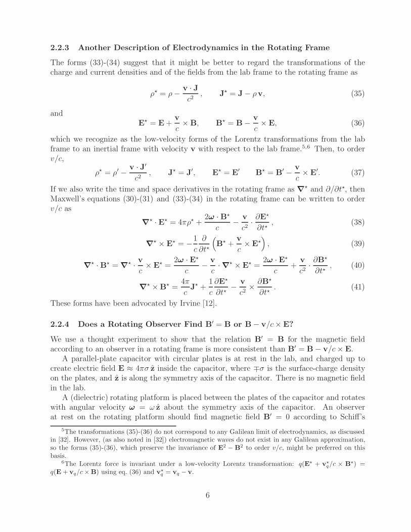
The forms (33)-(34) suggest that it might be better to regard the transformations of thecharge and current densities and of the fields from the lab frame to the rotating frame as
ρ� = ρ − v · Jc2
, J� = J − ρv, (35)
andE� = E +
v
c× B, B� = B − v
c× E, (36)
which we recognize as the low-velocity forms of the Lorentz transformations from the labframe to an inertial frame with velocity v with respect to the lab frame.5,6 Then, to orderv/c,
ρ� = ρ′ − v · J′
c2, J� = J′, E� = E′ B� = B′ − v
c× E′. (37)
If we also write the time and space derivatives in the rotating frame as ∇� and ∂/∂t�, thenMaxwell’s equations (30)-(31) and (33)-(34) in the rotating frame can be written to orderv/c as
∇� · E� = 4πρ� +2ω · B�
c− v
c2· ∂E�
∂t�, (38)
∇� × E� = −1
c
∂
∂t�
(B� +
v
c× E�
), (39)
∇� · B� = ∇� · v
c× E� =
2ω · E�
c− v
c· ∇� × E� =
2ω · E�
c+
v
c2· ∂B�
∂t�, (40)
∇� ×B� =4π
cJ� +
1
c
∂E�
∂t�− v
c2× ∂B�
∂t�. (41)
These forms have been advocated by Irvine [12].
2.2.4 Does a Rotating Observer Find B′ = B or B − v/c× E?
We use a thought experiment to show that the relation B′ = B for the magnetic fieldaccording to an observer in a rotating frame is more consistent than B′ = B − v/c × E.
A parallel-plate capacitor with circular plates is at rest in the lab, and charged up tocreate electric field E ≈ 4πσ z inside the capacitor, where ∓σ is the surface-charge densityon the plates, and z is along the symmetry axis of the capacitor. There is no magnetic fieldin the lab.
A (dielectric) rotating platform is placed between the plates of the capacitor and rotateswith angular velocity ω = ω z about the symmetry axis of the capacitor. An observerat rest on the rotating platform should find magnetic field B′ = 0 according to Schiff’s
5The transformations (35)-(36) do not correspond to any Galilean limit of electrodynamics, as discussedin [32]. However, (as also noted in [32]) electromagnetic waves do not exist in any Galilean approximation,so the forms (35)-(36), which preserve the invariance of E2 − B2 to order v/c, might be preferred on thisbasis.
6The Lorentz force is invariant under a low-velocity Lorentz transformation: q(E� + v�q/c × B�) =
q(E + vq/c ×B) using eq. (36) and v�q = vq − v.
6

transformation (10),7 but the magnetic field inside the capacitor should be B� = −v/c×E =ωEr r/c (in cylindrical coordinates) according to eq. (37). In both prescriptions the electricfield in the rotating frame is the same as that in the lab, E = E′ = E�.
Consider an electron of charge e that is released from rest in the lab on the upper plateof the capacitor. The electron accelerates straight downwards in the lab.
In the rotating frame, the electron has uniform circular motion in the plane of the plates,as well as downwards acceleration.
This motion is consistent with Schiff’s view that there is no magnetic field in the rotatingframe.
In view of sec. 2.2.3, the downward velocity, v�z of the electron combines with the radial
magnetic field B� to give an azimuthal component of the Lorentz force, Fφ = ev�zB
�/c =ev�
zωrE/c2. While ωr � c, we do not require that v�z � c, since the voltage between the
plates could be, say, 1 million volts, so that v�z ≈ c as the electron nears the lower plate.
Then, Fφ can be of order eE(ωr/c), which is not negligible. As a result, the electron’sazimuthal velocity would not maintain the expected constant value of −ωr.
Thus, there is an inconsistency at order v/c in the description according to sec. 2.2.3,which argues that Schiff’s formulation is the more “realistic”, despite the appearance of“fictitious” currents.
We shall see in the Appendix that Schiff’s forms correspond to use of the covariantelectromagnetic field tensors, while the forms B� = B−v/c×E (together with E� = E) arecomponents of the contravariant field tensor in the rotating frame, for which the form of theLorentz force is altered slightly from its familiar form. Consistent dynamics can be achievedwith these forms in the rotating frame by introduction of a “fictitious” term in the Lorentzforce law, as discussed in sec. A.4.
2.2.5 Summary of Electrodynamics in a Rotating Frame
For reference, we reproduce the principles of electrodynamics in the frame of a slowly rotatingmedium where ε and μ differ from unity.8 These relations are derived in the Appendix, notingthat the electromagnetic fields in the rotating frame summarized below are the covariantfields, the Lorentz force vector is the covariant force vector, but the velocity vector v′ is thecontravariant velocity and the charge and current densities ρ′ and J′ are the contravariantcomponents of the 4-current. Extreme care is required when making a “covariant” analysisin the rotating frame, because, for example, a particle at rest in the rotating frame is to bedescribed as having a nonzero covariant 3-velocity (sec. A.3.1), and use of the contravariantderivative operator does not lead to meaningful physics relations (sec. A.3.4).
The (cylindrical) coordinate transformation is
r′ = r, φ′ = φ − ωt, z′ = z, t′ = t, (42)
7The capacitor plates rotate with angular velocity −ω with respect to the rotating frame, where therotating charge density ρ′ = ρ leads to a surface current J′ = −ρ′ v according to Schiff. However, there arealso “fictitious” currents in Schiff’s prescription, given by ∇′ × (v × E′)/4π = (∇′ · E′)v/4π = ρ′ v = −J′,so the total current is zero and B′ = 0.
8This case is discussed most thoroughly by Ridgely [27, 29], but primarily for the interesting limit ofsteady charge and current distributions.
7

where quantities in observed in the rotating frame are labeled with a ′. The transformationsof charge and current density are
ρ′ = ρ, J′ = J − ρv, (43)
where v (v � c) is the velocity with respect to the lab frame of the observer in the rotatingframe. The transformations of the electromagnetic fields are
B′ = B, D′ = D +v
c× H, E′ = E +
v
c× B, H′ = H. (44)
The transformations of the electric and magnetic polarizations are
P′ = P− v
c× M, M′ = M, (45)
if we regard these polarizations as defined by D′ = E′ + 4πP′ and B′ = H′ + 4πM′.The lab-frame bound charge and current densities ρbound = −∇ ·P and Jbound = ∂P/∂t+
c∇ × M transform to9
ρ′bound = −∇′ · P′ − 2ω · M′
c+
v
c· ∇′ ×M′, (46)
J′bound =
∂P′
∂t′+ c∇′ × M′ + v(∇′ · P′) +
v
c× ∂M′
∂t′+ ω × P′ − ω
∂P′
∂φ′ . (47)
Force F is invariant under the transformation (42). In particular, a charge q with velocityvq in the lab frame experiences a Lorentz force in the rotating frame given by
F′ = q
(E′ +
v′q
c× B′
)= q
(E +
vq
c× B
)= F, (48)
where v′q = vq −v. Similarly, the Lorentz force density f ′ on charge and current densities in
the rotating frame is
f ′ = ρ′E′ +J′
c× B′ = (ρ′
free + ρ′bound) E′ +
J′free + J′
bound
c× B′. (49)
Maxwell’s equations in the rotating frame can be written
∇′ · B′ = 0, (50)
∇′ · D′ = 4πρ′free,total = 4π (ρ′
free + ρ′other) , (51)
∇′ × E′ +∂B′
∂ct′= 0, (52)
∇′ × H′ − ∂D′
∂ct′=
4π
cJ′
free,total =4π
c(J′
free + J′other) , (53)
9The term −2ω · M′/c is in effect a charge density −∇′ · P′mag associated with an electric polarization
density P′mag that appears along with magnetization in a rotating frame [33].
8

where ρ′free = ρfree and J′
free = Jfree − ρfreev are the free charge and current densities, and the“other” charge and current densities that appear to an observer in the rotating frame are
ρ′other = −v · J′
free
c2+
ω · H′
2πc− v
4πc· ∂D′
∂ct′, (54)
J′other = ρ′
freev + ω × D′
4π− ω
4π
∂D′
∂φ′ −v
4πc× ∂H′
∂t′. (55)
The “other” charge and current distributions are sometimes called “fictitious” [6], but wefind this term misleading.10 For an example with an “other” charge density ω · H′/2πc inthe rotating frame, see [35].
Maxwell’s equations can also be expressed only in terms of the fields E′ and B′ andcharge and current densities associated with free charges as well as with electric and magneticpolarization:
∇′ · E′ = 4πρ′total, (56)
and
∇′ × B′ − ∂E′
∂ct′=
4π
cJ′
total, (57)
where
ρ′total = ρ′
free −v
c2· J′
free −∇′ · P′ +ω · H′
2πc− v
4πc· ∂D′
∂ct′= ρ′
free,total − ∇′ · P′
= ρ′free + ρ′
bound + ρ′more , (58)
ρ′more = − v
c2·(J′
free +∂P′
∂t′+ c∇′ × M′
)+
ω · B′
2πc− v
4πc· ∂E′
∂ct′, (59)
J′total = J′
free +∂P′
∂t′+ c∇′ × M′ + ρ′
freev + ω × D′
4π− ω
4π
∂D′
∂φ′ −v
4πc× ∂H′
∂t′
= J′free,total +
∂P′
∂t′+ c∇′ × M′
= J′free + J′
bound + J′more , (60)
J′more = v
(ρ′
free − ∇′ · P′ − 2ω ·M′
c+
v
c· ∇′ × M′
)
+ω × E′
4π− ω
4π
∂E′
∂φ′ −v
4πc× ∂B′
∂t′. (61)
The contribution of the polarization densities to the source terms in Maxwell’s equations inmuch more complex in the rotating frame than in the lab frame.11 Because of the “other”source terms that depend on the fields in the rotating frame, Maxwell’s equations cannot besolved directly in this frame. Rather, an iterative approach is required in general.
10According to Einstein [34], “fields which can be transformed into each other by such transformations[as eq. (42)] describe the same real situation.” In particular, the “fictitious” sources (54)-(55) are an aspectof a description by an observer in the rotating frame of the same physical situation as observed in the labframe.
11Neglect of this complexity can lead to apparent paradoxes involving rotating magnetic media [11, 25].
9

The constitutive equations for a linear, isotropic medium at rest in the rotating frameare12
D′ = εE′, B′ = μH′ − (εμ − 1)v
c× E′, (62)
in the rotating frame, and
D = εE + (εμ − 1)v
c× H, B = μH − (εμ − 1)
v
c× E, (63)
in the lab frame, where ε and μ are the permittivity and permeability of the medium whenat rest in an inertial frame. The lab-frame constitutive equations (63) are the same as for anonrotating medium that moves with constant velocity v with respect to the lab frame.
We can also write the constitutive equations (62) for a linear, isotropic medium in termsof the fields B′, E′, P′ and M′ by noting that D′ = E′ + 4πP′ and H′ = B′ − 4πM′, so that
P′ =ε − 1
4πE′,
M′ =
(1 − 1
μ
)B′
4π−(
ε − 1
μ
)v
c× E′
4π=
(1 − 1
μ
)B′
4π− εμ − 1
μ(ε− 1)
v
c× P′. (64)
Similarly, the constitutive equations (63) in the lab frame can be written to order v/c as
P =ε − 1
4πE +
(ε − 1
μ
)v
c× B
4π=
ε − 1
4πE +
εμ − 1
μ − 1
v
c× M,
M =
(1 − 1
μ
)B
4π−(
ε − 1
μ
)v
c× E
4π=
(1 − 1
μ
)B
4π− εμ − 1
μ(ε− 1)
v
c× P. (65)
Ohm’s law for the conduction current JC has the same form for a medium with velocityu′ relative to the rotating frame as it does for a medium with velocity u relative to the labframe,
J′C = σ
(E′ +
u′
c× B′
)= σ
(E +
u
c× B
)= JC, (66)
where σ is the electric conductivity of a medium at rest in an inertial frame.
A Appendix: Electrodynamics Using Covariant and
Contravariant Vectors and Tensors
In the preceding we have used only vector notation when discussing electrodynamics, eventhough it is more proper to consider the vector fields B and E as part of a field tensorF. Furthermore, one should distinguish between covariant and contravariant vectors andtensors.
In an inertial frame, the distinction between covariant and contravariant vectors is rathertrivial, so that one can neglect this distinction and then speak of the field vectors B andE without confusion. However, the metric tensor is not diagonal in a rotating frame, so
12Different constitutive equations hold for a rotating permanent magnet [36] or for a rotating electret.
10

that greater care should be made in distinguishing covariant and contravariant vectors andtensors [24, 29].
The summary of electrodynamics in a rotating frame given in sec. 2.2.5 does not mentioncovariant and contravariant components, and simply uses a ′ to indicate quantities observedin the rotating frame. As shown in this Appendix, it is consistent to make such a summaryif one obeys the following conventions,
1. All components of electromagnetic field vectors B′, D′, E′, H′, P′ and M′ that appearin sec.2.2.5 are components of their respective covariant tensors.
2. The gradient operator ∇′ is part of the covariant 4-derivative operator.
3. The velocity u′, and the charge and current densities ρ′, ρ′free, J′ and J′
free are con-travariant components of their respective contravariant 4-vectors.13
4. The bound charge and current densities ρ′bound and J′
bound are representations of theircontravariant 4-vectors in terms of covariant components of the relevant electromag-netic fields.
These conventions are relatively straightforward except for item 4, which is needed so thatcharge conservation, ∇′·J′+∂ρ′/∂t′ = 0, holds for bound as well was for free charge, while ob-serving the convention that electromagnetic fields are represented by covariant components.For examples exhibiting charge conservation in rotating media, see [5, 36].
A.1 Notation
We will indicate a contravariant 4-vector or 4-tensor by indices that are Greek superscripts,and covariant 4-vector or 4-tensor by indices that are Greek subscripts.14 The componentsof contravariant 4-vectors and tensors (other than the position 4-vector xα) will have a ˜above the symbol. Quantities measured in the rotating frame will be designated with a′. As before, we only consider velocities small compared to the speed of light. The vectorv = ω × x is the velocity in the (inertial) lab frame of a point at position x that is at restin the rotating frame, whose angular velocity is ω = ω z with respect to the lab frame.
The metric tensor for rectangular coordinates in an inertial frame is written
gαβ = gαβ =
⎛⎜⎜⎜⎜⎜⎜⎝
1 0 0 0
0 −1 0 0
0 0 −1 0
0 0 0 −1
⎞⎟⎟⎟⎟⎟⎟⎠
, (67)
where the Greek indices run from 0 to 3 (and we ignore the effect of gravity on electrody-namics).
13In this Appendix, components of contravariant vectors and tensors will include a ˜ above the symbol.14The notion of covariant and contravariant vectors and tensors arises from the character of their trans-
formations from one frame to another. We defer discussion of details of these transformations until sec. A.3.
11
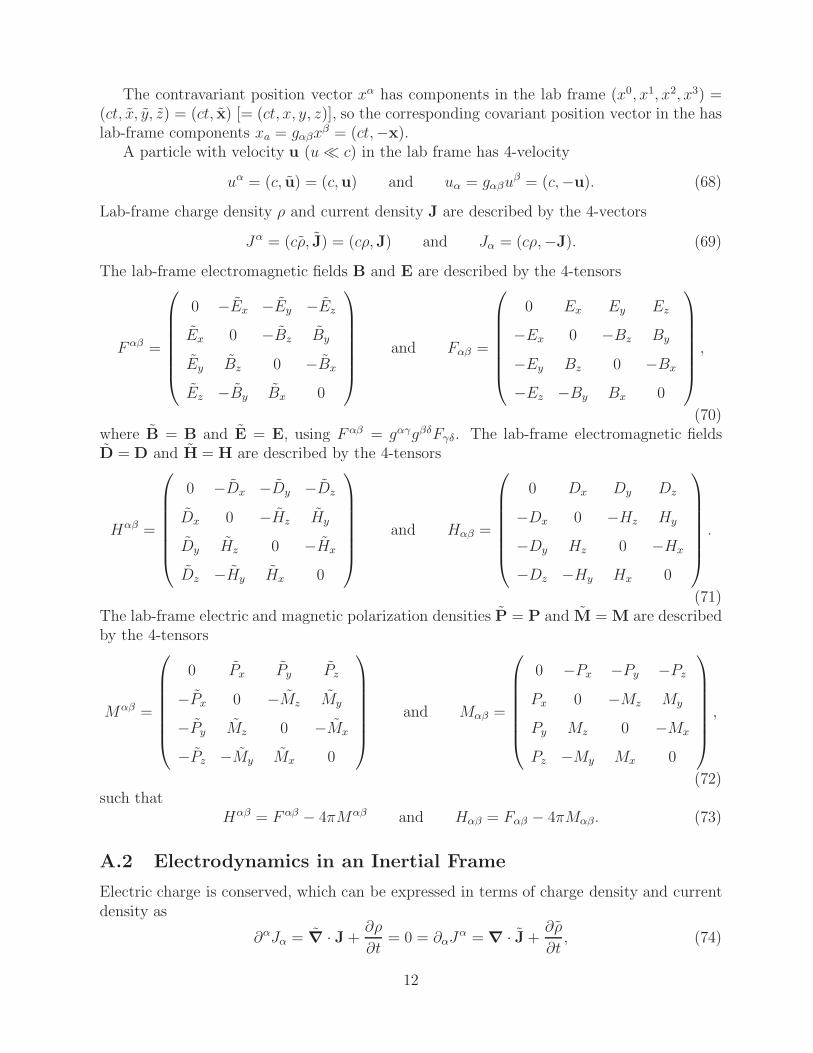
The contravariant position vector xα has components in the lab frame (x0, x1, x2, x3) =(ct, x, y, z) = (ct, x) [= (ct, x, y, z)], so the corresponding covariant position vector in the haslab-frame components xa = gαβx
β = (ct,−x).A particle with velocity u (u � c) in the lab frame has 4-velocity
uα = (c, u) = (c,u) and uα = gαβuβ = (c,−u). (68)
Lab-frame charge density ρ and current density J are described by the 4-vectors
Jα = (cρ, J) = (cρ,J) and Jα = (cρ,−J). (69)
The lab-frame electromagnetic fields B and E are described by the 4-tensors
F αβ =
⎛⎜⎜⎜⎜⎜⎜⎝
0 −Ex −Ey −Ez
Ex 0 −Bz By
Ey Bz 0 −Bx
Ez −By Bx 0
⎞⎟⎟⎟⎟⎟⎟⎠
and Fαβ =
⎛⎜⎜⎜⎜⎜⎜⎝
0 Ex Ey Ez
−Ex 0 −Bz By
−Ey Bz 0 −Bx
−Ez −By Bx 0
⎞⎟⎟⎟⎟⎟⎟⎠
,
(70)where B = B and E = E, using F αβ = gαγgβδFγδ. The lab-frame electromagnetic fieldsD = D and H = H are described by the 4-tensors
Hαβ =
⎛⎜⎜⎜⎜⎜⎜⎝
0 −Dx −Dy −Dz
Dx 0 −Hz Hy
Dy Hz 0 −Hx
Dz −Hy Hx 0
⎞⎟⎟⎟⎟⎟⎟⎠
and Hαβ =
⎛⎜⎜⎜⎜⎜⎜⎝
0 Dx Dy Dz
−Dx 0 −Hz Hy
−Dy Hz 0 −Hx
−Dz −Hy Hx 0
⎞⎟⎟⎟⎟⎟⎟⎠
.
(71)The lab-frame electric and magnetic polarization densities P = P and M = M are describedby the 4-tensors
Mαβ =
⎛⎜⎜⎜⎜⎜⎜⎝
0 Px Py Pz
−Px 0 −Mz My
−Py Mz 0 −Mx
−Pz −My Mx 0
⎞⎟⎟⎟⎟⎟⎟⎠
and Mαβ =
⎛⎜⎜⎜⎜⎜⎜⎝
0 −Px −Py −Pz
Px 0 −Mz My
Py Mz 0 −Mx
Pz −My Mx 0
⎞⎟⎟⎟⎟⎟⎟⎠
,
(72)such that
Hαβ = F αβ − 4πMαβ and Hαβ = Fαβ − 4πMαβ. (73)
A.2 Electrodynamics in an Inertial Frame
Electric charge is conserved, which can be expressed in terms of charge density and currentdensity as
∂αJα = ∇ · J +∂ρ
∂t= 0 = ∂αJα = ∇ · J +
∂ρ
∂t, (74)
12

where ∇ = ∇ and
∂α =∂
∂xα
=
(∂
∂ct,−∇
)and ∂α =
∂
∂xα
=
(∂
∂ct, ∇)
. (75)
The Lorentz force f on a charge q that moves with velocity u in the lab frame is describedby the 4-vectors
fα = (f · u/c, f ) = qF αβuβ = q(E · u/c, E + u/c × B), (76)
fα = (f · u/c,−f) = qFαβuβ = q(E · u/c,−E − u/c × B). (77)
In inertial frames we can ignore the fact that the Lorentz force vector is composed of a mixof covariant and contravariant vectors.
The two Maxwell’s equations for B and E that involve the total charge density ρ and thetotal current density J,
∇ · E = 4πρ = 4πρ = ∇ · E, ∇ × B − ∂E
∂ct=
4π
cJ =
4π
cJ = ∇ × B − ∂E
∂ct, (78)
can be written as15
∂αF αβ =4π
cJβ or ∂αFαβ =
4π
cJβ , (80)
while the other two Maxwell’s equations,
∇ · B = ∇ · B = 0, ∇× E +∂B
∂ct= ∇ × E +
∂B
∂ct= 0, (81)
can be written as∂αFαβ = 0 or ∂αFαβ = 0, (82)
where the dual of an antisymmetric, covariant tensor Fαβ is the contravariant tensor F αβ
defined by
Fαβ =1
2εαβγδFγδ =
⎛⎜⎜⎜⎜⎜⎜⎝
0 −Bx −By −Bz
Bx 0 Ez −Ey
By −Ez 0 Ex
Bz Ey −Ex 0
⎞⎟⎟⎟⎟⎟⎟⎠
(83)
when the components of tensor Fαβ are defined as in eq. (70), and where
εαβγδ = −εαβγδ =
⎧⎪⎪⎪⎨⎪⎪⎪⎩
+1 if αβγδ is an even permutation of 0123,
−1 if αβγδ is an odd permutation of 0123,
0 if any two indices are equal.
(84)
15The field tensors can be derived from 4-potentials according to
F αβ = ∂αAβ − ∂βAα, Aα = (V , A) = (V, A), Fαβ = ∂αAβ − ∂βAα, Aα = (V,−A). (79)
13

Similarly, we define
Fαβ =1
2εαβγδF
γδ =
⎛⎜⎜⎜⎜⎜⎜⎝
0 Bx By Bz
−Bx 0 Ez −Ey
−By −Ez 0 Ex
−Bz Ey −Ex 0
⎞⎟⎟⎟⎟⎟⎟⎠
. (85)
The components of the dual tensor Fαβ can be obtained from those of F αβ by the dualitytransformation
E → B, B → −E (F αβ → Fαβ), (86)
while those of the dual tensor Fαβ can be obtained from those of Fαβ by the transformation
E → B, B → −E (Fαβ → Fαβ). (87)
If ρfree and Jfree represent only the free charge density and the conduction current, thenthe Maxwell equations
∇ · D = 4πρfree = 4πρfree = ∇ ·D, ∇× H− ∂D
∂ct=
4π
cJ =
4π
cJ = ∇×H− ∂D
∂ct, (88)
can be written as
∂αHαβ =4π
cJβ
free or ∂αHαβ =4π
cJfreeβ . (89)
It is not obvious from the preceding how the alternative forms of Maxwell’s equations(82) and (89) should be paired. However, once we consider transformations to noninertialframes it becomes clear that the pairing must be
∂αFαβ = 0 and ∂αHαβ =4π
cJfreeβ, (90)
or
∂αFαβ = 0 and ∂αHαβ =4π
cJβ
free. (91)
This has the implication that when Maxwell’s equations are expressed in terms of covariantand contravariant 3-vectors B, D, E and H and B, D, E and H they have the mixed forms
∇ · D = 4πρfree, ∇× E +∂B
∂ct= 0, ∇ · B = 0, ∇× H − ∂D
∂ct=
4π
cJfree, (92)
or
∇ · D = 4πρfree, ∇× E +∂B
∂ct= 0, ∇ · B = 0, ∇× H − ∂D
∂ct=
4π
cJfree. (93)
Since there is no difference between covariant and contravariant components in inertialframes, the mixing seen in eqs. (92)-(93) goes unnoticed there.
14

The relation between the total and free charge and current densities can be written as
ρ = ρfree − ∇ · P, J = Jfree +∂P
∂t+ c∇ × M,
or ρ = ρfree − ∇ · P, J = Jfree +∂P
∂t+ c ∇ ×M. (94)
or in 4-vector form as
Jβ = Jβfree + c ∂αMαβ or Jβ = Jfreeβ + c ∂αMαβ , (95)
The constitutive equations,
D = D = εE = εE and B = B = μH = μH, (96)
hold only in an inertial rest frame of a linear, isotropic medium. If the medium has velocityu (u � c) with respect to the (inertial) lab frame, the constitutive equations in the lab frameare
D +v
c× H = ε
(E +
v
c× B
)and B − v
c× E = μ
(H− v
c× D
), (97)
or D +v
c× H = ε
(E +
v
c× B
)and B − v
c× E = μ
(H− v
c×D
), (98)
which can be expressed in tensor form as
Hαβuβ = εFαβuβ and Fαβu
β = μHαβuβ, (99)
or Hαβuβ = εF αβuβ and Fαβuβ = μHαβuβ, (100)
using the dual tensors introduced in eqs. (85)-(87), as first noted by Minkowski [3]. Thepairings in eqs. (99)-(100) follow those made for Maxwell’s equations (90)-(91).
In the present case of a medium that is at rest in a rotating frame, the constitutiveequations (97)-(98) hold in the lab frame, since these relations summarize physical effectsin a very small region about the point of observation, for which a Lorentz transformationbetween the lab frame and the comoving local inertial frame of a point at rest in the rotatingframe provides an adequate description. A remaining issue is the form of the constitutiveequations in the noninertial rotating frame. This technical issue is not relevant to an analysisof quantities in the lab frame, as observed, for example, in the Wilson-Wilson experiment[4, 5].
A third constitutive equation is Ohm’s law for the conduction current JC , which has theform
JC = σE (101)
in the rest frame of a medium with DC conductivity σ. We consider only the case ofconduction currents in a neutral medium, so that their is no net charge density associatedwith the conduction current.16 Then, it is consistent to write Ohm’s law in a form similarto that of the Lorentz force law (77),
JαC = (JC · u/c, JC) = σF αβuβ = σ(E · u/c, E + u/c × B), (102)
JCα = (JC · u/c,−JC) = σFαβuβ = σ(E · u/c,−E − u/c ×B), (103)
16See prob. 11.16 of [37] for the case when convection currents are present.
15

where u is the velocity of the conductor relative to the lab frame. Thus, the conductioncurrent is
JC = σ(E +
u
c× B
)= σ
(E +
u
c× B
)= JC (104)
in a moving conductor. There is little physical significance to the time components σE ·u/cand σE · u/c in the case of a moving conductor. For a more general discussion, see [38].
A.3 Transformations from Lab to Rotating Frame
The (cylindrical) coordinates in the rotating frame (denoted with a ′) are related to those inthe lab frame by
t′ = t, r′ = r, φ′ = φ − ωt, z′ = z, (105)
so the contravariant, rectangular coordinate transformation is
x′0 = x0, x′1 = x1 cosω
cx0 + x2 sin
ω
cx0, x′2 = −x1 sin
ω
cx0 + x2 cos
ω
cx0, x′3 = x3,
(106)whose inverse is
x0 = x′0, x1 = x′1 cosω
cx′0 − x′2 sin
ω
cx′0, x2 = x′1 sin
ω
cx′0 + x′2 cos
ω
cx′0, x3 = x′3.
(107)A contravariant 4-vector Aα transforms according to
A′α =∂x′α
∂xβAβ, (108)
while a covariant 4-vector Aα transforms according to
A′α =
∂xβ
∂x′α Aβ. (109)
When writing ∂x′α/∂xβ and ∂xβ/∂x′α as matrices (and Aα and Aα as column vectors),indices α and β label the rows and columns, respectively.
A.3.1 Covariant Vectors and Tensors in the Rotating Frame
To transform covariant vectors and tensors from the lab frame to the rotating frame we use
∂xβ
∂x′α =
⎛⎜⎜⎜⎜⎜⎜⎝
1 vx
cvy
c0
0 cos ωcx0 − sin ω
cx0 0
0 sin ωcx0 cos ω
cx0 0
0 0 0 1
⎞⎟⎟⎟⎟⎟⎟⎠
=
⎛⎜⎜⎜⎜⎜⎜⎝
1 vx
cvy
c0
0 1 0 0
0 0 1 0
0 0 0 1
⎞⎟⎟⎟⎟⎟⎟⎠
⎛⎜⎜⎜⎜⎜⎜⎝
1 0 0 0
0 cos ωcx0 − sin ω
cx0 0
0 sin ωcx0 cos ω
cx0 0
0 0 0 1
⎞⎟⎟⎟⎟⎟⎟⎠
,
(110)where v = (vx, vy, 0) = (−ωy, ωx, 0) is the velocity in the lab frame of the point x′ in therotating frame. The transformation (110) is composed of a rotation about the z axis and
16
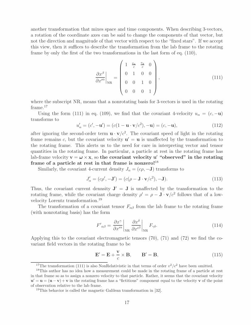
another transformation that mixes space and time components. When describing 3-vectors,a rotation of the coordinate axes can be said to change the components of that vector, butnot the direction and magnitude of that vector with respect to the “fixed stars”. If we acceptthis view, then it suffices to describe the transformation from the lab frame to the rotatingframe by only the first of the two transformations in the last form of eq. (110),
∂xβ
∂x′α
∣∣∣∣NR
=
⎛⎜⎜⎜⎜⎜⎜⎝
1 vx
c
vy
c0
0 1 0 0
0 0 1 0
0 0 0 1
⎞⎟⎟⎟⎟⎟⎟⎠
, (111)
where the subscript NR, means that a nonrotating basis for 3-vectors is used in the rotatingframe.17
Using the form (111) in eq. (109), we find that the covariant 4-velocity uα = (c,−u)transforms to
u′α = (c′,−u′) = (c(1 − u · v/c2),−u) = (c,−u), (112)
after ignoring the second-order term u · v/c2. The covariant speed of light in the rotatingframe remains c, but the covariant velocity u′ = u is unaffected by the transformation tothe rotating frame. This alerts us to the need for care in interpreting vector and tensorquantities in the rotating frame. In particular, a particle at rest in the rotating frame haslab-frame velocity v = ω×x, so the covariant velocity u′ “observed” in the rotatingframe of a particle at rest in that frame is nonzero!18
Similarly, the covariant 4-current density Jα = (cρ,−J) transforms to
J ′α = (cρ′,−J′) = (c(ρ − J · v/c2),−J). (113)
Thus, the covariant current dennsity J′ = J is unaffected by the transformation to therotating frame, while the covariant charge density ρ′ = ρ − J · v/c2 follows that of a low-velocity Lorentz transformation.19
The transformation of a covariant tensor Fαβ from the lab frame to the rotating frame(with nonrotating basis) has the form
F ′αβ =
∂xγ
∂x′α
∣∣∣∣NR
∂xδ
∂x′β
∣∣∣∣NR
Fγδ. (114)
Applying this to the covariant electromagnetic tensors (70), (71) and (72) we find the co-variant field vectors in the rotating frame to be
E′ = E +v
c× B, B′ = B, (115)
17The transformation (111) is also NonRelativistic in that terms of order v2/c2 have been omitted.18This author has no idea how a measurement could be made in the rotating frame of a particle at rest
in that frame so as to assign a nonzero velocity to that particle. Rather, it seems that the covariant velocityu′ = u = (u− v)+ v in the rotating frame has a “fictitious” component equal to the velocity v of the pointof observation relative to the lab frame.
19This behavior is called the magnetic Galilean transformation in [32].
17

D′ = D +v
c× H, H′ = H, (116)
andP′ = P− v
c× M, M′ = M. (117)
A.3.2 Contravariant Vectors and Tensors in the Rotating Frame
We now have two methods to obtain the forms of contravariant vectors and tensors in therotating frame. We can use eq. (108) to go directly from the lab frame to the rotating frame,once we have found the version of ∂x′α/∂xβ that applies to a nonrotating basis in the rotatingframe. Or, we can use the metric tensor g′ in the rotating frame (once we have identifiedthis) to go from covariant to contravariant vectors and tensors in that frame according to
A′α = g′αβA′
β , F ′αβ= g′αγ
g′βδF ′
γδ. (118)
For these two approaches to be consistent, we need that
A′α = g′αβA′
β = g′αγ ∂xβ
∂x′γ
∣∣∣∣NR
Aβ = g′αγ ∂xδ
∂x′γ
∣∣∣∣NR
gδβAβ =
∂x′α
∂xβ
∣∣∣∣NR
Aβ, (119)
i.e., that∂x′α
∂xβ
∣∣∣∣NR
= g′αγ ∂xδ
∂x′γ
∣∣∣∣NR
gδβ. (120)
Recalling eq. (106), we have that
∂x′α
∂xβ=
⎛⎜⎜⎜⎜⎜⎜⎝
1 0 0 0
v′xc
cos ωcx0 sin ω
cx0 0
v′yc
− sin ωcx0 cos ω
cx0 0
0 0 0 1
⎞⎟⎟⎟⎟⎟⎟⎠
=
⎛⎜⎜⎜⎜⎜⎜⎝
1 0 0 0
v′xc
1 0 0v′yc
0 1 0
0 0 0 1
⎞⎟⎟⎟⎟⎟⎟⎠
⎛⎜⎜⎜⎜⎜⎜⎝
1 0 0 0
0 cos ωcx0 sin ω
cx0 0
0 − sin ωcx0 cos ω
cx0 0
0 0 0 1
⎞⎟⎟⎟⎟⎟⎟⎠
,
(121)where v′ = (v′
x, v′y, 0) = (ωy′,−ωx′, 0) is the velocity in the rotating frame of the point in
the lab frame whose present coordinates are x′ in the rotating frame. As before, we omitthe rotation so that vectors in the rotating frame are defined with respect to a nonrotatingbasis. Then velocity v′ = −v, where as before v is the velocity of point x′ with respect tothe lab frame. Hence,
∂x′α
∂xβ
∣∣∣∣NR
=
⎛⎜⎜⎜⎜⎜⎜⎝
1 0 0 0
− vx
c1 0 0
− vy
c0 1 0
0 0 0 1
⎞⎟⎟⎟⎟⎟⎟⎠
. (122)
To identify the metric tensor g′ we recall eqs. (105)-(106) to write the invariant intervalas
ds2 = d(x0)2 − d(x1)2 − d(x2)2 − d(x3)2 (123)
≈ d(x′0)2 − d(x′1)2 − d(x′2)2 − d(x′3)2 − 2ωx′2
cd(x′0)d(x′1) − 2
ωx′1
cd(x′0)d(x′2),
18

where we ignore a term of order ω2r2/c2.20 Thus, the (symmetric) metric tensor in therotating frame is
g′αβ = g′αβ ≈
⎛⎜⎜⎜⎜⎜⎜⎝
1 − vx
c− vy
c0
− vx
c−1 0 0
− vy
c0 −1 0
0 0 0 −1
⎞⎟⎟⎟⎟⎟⎟⎠
, (124)
where we again write (ωx′2,−ωx′1) as (−vx,−vy).21
As a check, we verify that
g′αγ ∂xδ
∂x′γ
∣∣∣∣NR
gδβ =
⎛⎜⎜⎜⎜⎜⎜⎝
1 − vx
c− vy
c0
− vx
c−1 0 0
− vy
c0 −1 0
0 0 0 −1
⎞⎟⎟⎟⎟⎟⎟⎠
⎛⎜⎜⎜⎜⎜⎜⎝
1 vx
c
vy
c0
0 1 0 0
0 0 1 0
0 0 0 1
⎞⎟⎟⎟⎟⎟⎟⎠
⎛⎜⎜⎜⎜⎜⎜⎝
1 0 0 0
0 −1 0 0
0 0 −1 0
0 0 0 −1
⎞⎟⎟⎟⎟⎟⎟⎠
=
⎛⎜⎜⎜⎜⎜⎜⎝
1 0 0 0
− vx
c1 0 0
− vy
c0 1 0
0 0 0 1
⎞⎟⎟⎟⎟⎟⎟⎠
=∂x′α
∂xβ
∣∣∣∣NR
, (125)
on neglect of terms of order v2/c2.Using the form (122) in eq. (108), we find that the contravariant 4-velocity uα = (c, u) =
(c,u) transforms to
u′α = (c′, u′) = (c, u− v) = (c,u− v) = g′αβu′
β. (126)
The contravariant speed of light remains c, and the contravariant velocity u′ = u−v behavesas expected for a low-velocity Lorentz transformation to the rotating frame. Thus, we mightfeel that the contravariant velocity is of greater physical significance than the covariantvelocity u′ = u in the rotating frame.
Similarly, the contravariant 4-current density Jα = (cρ, J) = (cρ,J) transforms to
J ′α = (cρ′, J′) = (cρ, J − ρv) = (cρ,J − ρv) = g′αβJ ′
β. (127)
The the contravariant charge density ρ′ = ρ is unaffected by the transformation to therotating frame, while the contravariant current density J′ = J − ρv follows that of a low-velocity Lorentz transformation.22
20By considering only radii where the velocity ωr is small compared to c we avoid difficulties such asEhrenfest’s paradox. For the latter, see [31].
21The determinant of g′ is unity, which excuses some glibness in the definition of the co- and contravariantderivative operators in eq. (75).
22This behavior is called the electric Galilean transformation in [32].
19
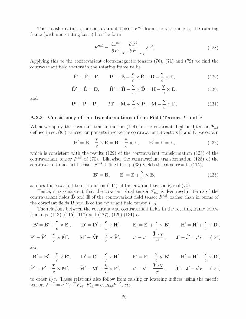
The transformation of a contravariant tensor F αβ from the lab frame to the rotatingframe (with nonrotating basis) has the form
F ′αβ=
∂x′α
∂xγ
∣∣∣∣NR
∂x′β
∂xδ
∣∣∣∣∣NR
F γδ. (128)
Applying this to the contravariant electromagnetic tensors (70), (71) and (72) we find thecontravariant field vectors in the rotating frame to be
E′ = E = E, B′ = B − v
c× E = B − v
c× E, (129)
D′ = D = D, H′ = H− v
c× D = H − v
c× D, (130)
andP′ = P = P, M′ = M +
v
c× P = M +
v
c× P, (131)
A.3.3 Consistency of the Transformations of the Field Tensors F and FWhen we apply the covariant transformation (114) to the covariant dual field tensor Fαβ
defined in eq. (85), whose components involve the contravariant 3-vectors B and E, we obtain
B′ = B − v
c× E = B − v
c× E, E′ = E = E, (132)
which is consistent with the results (129) of the contravariant transformation (128) of thecontravariant tensor F αβ of (70). Likewise, the contravariant transformation (128) of thecontravariant dual field tensor Fαβ defined in eq. (83) yields the same results (115),
B′ = B, E′ = E +v
c×B, (133)
as does the covariant transformation (114) of the covariant tensor Fαβ of (70).Hence, it is consistent that the covariant dual tensor Fαβ is described in terms of the
contravariant fields B and E of the contravariant field tensor F αβ , rather than in terms ofthe covariant fields B and E of the covariant field tensor Fαβ.
The relations between the covariant and contravariant fields in the rotating frame followfrom eqs. (113), (115)-(117) and (127), (129)-(131) as
B′ = B′ +v
c× E′, D′ = D′ +
v
c× H′, E′ = E′ +
v
c× B′, H′ = H′ +
v
c× D′,
P′ = P′ − v
c× M′, M′ = M′ − v
c× P′, ρ′ = ρ′ − J′ · v
c2, J′ = J′ + ρ′v, (134)
and
B′ = B′ − v
c× E′, D′ = D′ − v
c× H′, E′ = E′ − v
c× B′, H′ = H′ − v
c× D′,
P′ = P′ +v
c× M′, M′ = M′ +
v
c×P′, ρ′ = ρ′ +
J′ · vc2
, J′ = J′ − ρ′v, (135)
to order v/c. These relations also follow from raising or lowering indices using the metrictensor, F ′αβ = g′αγg′βδF ′
γδ, F ′αβ = g′
αγg′βδF
′γδ, etc.
20

A.3.4 The Derivative Operators ∂ ′α and ∂ ′α in the Rotating Frame
If we regard the lab-frame derivative operators ∂ ′α and ∂ ′α, defined in eq. (75), as 4-vectors
then we expect that their forms in the rotating frame could be written
∂ ′α =
(∂
∂ct′, ∇′
)=
(∂
∂ct+
v
c· ∇, ∇
)and ∂ ′α =
(∂
∂ct′,−∇′
)=
(∂
∂ct,−∇− v
c
∂
∂ct
),
(136)recalling the transformations (111) and (122). Thus, we are led to two different meanings ofthe operator ∂/∂t′. To determine whether either of the operations ∂ ′
α and ∂ ′α is meaningful,we consider whether they imply that charge is conserved in the rotating frame:
∂ ′αJ ′α = ∇′ · J′ +
∂ρ′
∂t′= ∇ · J − ∇ · ρv +
∂ρ
∂t+ (v · ∇)ρ = ∇ · J +
∂ρ
∂t= 0, (137)
noting that ∇ · ρv = (v ·∇)ρ since ∇ · v = 0 according to eq. (19). However,
∂ ′αJ ′α = ∇′ · J′ +
∂ρ′
∂t′= ∇ · J +
v
c
∂J
∂ct+
∂ρ
∂t− ∂J · v/c
ct= ∇ · J +
∂ρ
∂t− J · ∂v/c
ct
= −J · ∂v/c
ct�= 0, (138)
since v is the lab-frame velocity of a point that is at rest in the rotating frame.Hence, it appears that we can use the covariant derivative operator ∂ ′
α, but not thecontravariant derivative operator ∂ ′α, to obtain meaningful physical results in the rotatingframe. This issue has been discussed in greater detail by Crater [24]. A consequence of thisis that Maxwell’s equations should be expressed in the rotating frame only in terms of thecovariant derivative operator (sec. A.6).
A.3.5 The Relation between Free, Bound and Total Charge and CurrentDensities in the Rotating Frame
While we might expect the relations (95) between the lab-frame free and total23 charge andcurrent densities would transform to
J ′β = J ′βfree + c ∂ ′
αM ′αβor J ′
β = J ′freeβ + c ∂ ′αM ′
αβ, (139)
in the rotating frame, we understand from sec. A.3.4 that only the contravariant currentdensity J ′α will be physical when nonzero electric or magnetic polarization are present. Thecovariant current density will be nonphysical (when nonzero electric or magnetic polarizationare present) due to the bad behavior of the contravariant derivative operator ∂ ′α. Hence, itis better to avoid use of the covariant components of polarization in the rotating frame whenrelating polarization to sources of the electromagnetic fields.
The relation between the contravariant total and free charge and current densities canbe written as
ρ′ = ρ′free + ρ′
bound, J′ = J′free + J′
bound (140)
23In sec. A.6 we will be led to a more general concept of the total charge and current densities in therotating frame than that implied by eq. (139).
21

where
ρ′bound = −∇′ · P′, J′
bound =∂P′
∂t′+ c∇′ × M′. (141)
We can verify that eq. (140) is consistent with the transformations (127), (131) and (136),
ρ = ρ′ = ρ′free − ∇′ · P′ = ρfree − ∇ · P, (142)
J′ = J − ρv = Jfree +∂P
∂t+ c∇ × M − ρfreev + v(∇ · P)
= J′free +
∂P′
∂t′+ c∇′ × M′
= Jfree − ρfreev +∂P
∂t+ v(∇ · P) − ∇ × (v × P) + c∇ × M + ∇ × (v × P)
= Jfree +∂P
∂t+ c∇ × M − ρfreev + v(∇ · P), (143)
where we have used the (subtle) relation (23) between the time derivatives ∂P′/∂t′ = ∂P/∂t′
and ∂P/∂t.Despite the difficulty in using eq. (139) to define covariant components of bound charge
and current densities, we will find ourselves desiring expressions for them. Therefore, we usethe relations (134)-(135) to convert the contravariant bound charge and current densities(141) to covariant components (to order v/c),
ρ′bound = ρ′
bound −v
c2· J′
bound = −∇′ · P′ − v
c2·(
∂P′
∂t′+ c∇′ × M′
)
= −∇′ · P′ − ∇′ ·(v
c× M′
)− v
c2·(
∂P′
∂t′+ c∇′ × M′
)(144)
= −∇′ · P′ − 2ω · M′
c− v
c2· ∂P′
∂t′,
J′bound = J′
bound + ρ′boundv =
∂P′
∂t′+ c∇′ × M′ − v(∇′ · P′)
=∂P′
∂t′+ c∇′ × M′ +
v
c× ∂M′
∂t′+ ∇′ × (v × P′) − v(∇′ · P′)
=∂P′
∂t′+ c∇′ × M′ +
v
c× ∂M′
∂t′+ ω × P′ − ω
∂P′
∂φ′ , (145)
recalling eqs. (13) and (22). These forms are counterintuitive, but they are consistent withtransforming the lab-frame bound charge and current densities ρbound = −∇ ·P and Jbound =∂P/∂t + c∇ × M to the rotating frame using eqs. (23) and (117).
For later use we record the relation between the contravariant and covariant charge andcurrent densities in the rotating frame, following eq. (135),
ρ′bound = ρ′
bound +v
c2· J′
bound = −∇′ · P′ − 2ω · M′
c+
v
c· ∇′ × M′, (146)
J′bound = J′
bound − ρ′boundv
=∂P′
∂t′+ c∇′ × M′ + v(∇′ · P′) +
v
c× ∂M′
∂t′+ ω × P′ − ω
∂P′
∂φ′ . (147)
22

The forms (140) and (144)-(147) reinforce that the contravariant forms of charge and currentdensities in the rotating frame, as expressed in terms of contravariant field components(140) correspond most closely to our experience in inertial frames. Both the covariant forms(144)-(145) and the contravariant forms (146)-(147) expressed in terms of covariant fieldcomponents include terms whose significance is not immediately evident. From Newtonianmechanics in rotating frames, we are used to the notion of “fictitious” forces that appear“real” to observers at rest in the rotating frame. The electrodynamics of rotating systemsis even more complex in that it leads us to multiple expressions for physical quantities, andthese are especially intricate in the case of bound charge and current densities.
The form (146) for the contravariant charge density in terms of covariant componentsindicates that magnetization in the rotating frame is associated with a bound charge distri-bution. This gives another perspective on the well-known result (see, for example, sec. 88 of[39], sec. 18-6 of [40] and also [36]24 ) that a nonzero bound charge density in the lab frameis associated with moving/rotating magnetization.
A.4 Lorentz Force and Ohm’s Law in the Rotating Frame
Now that we have expressions for both covariant and contravariant vectors and tensors inthe rotating frame, we can evaluate the Lorentz force on a charge q there.
The contravariant Lorentz force in the rotating frame is
f ′α = qF ′αβu′
β = q(E′ · u′/c, E′ + u′/c × B′) = q(E · u/c,E + u/c × B), (148)
plus terms of order uv/c2. The contravariant 3-vector Lorentz force in the rotating frame is
f ′ = q
(E′ +
u′
c× B′
)= q
(E +
u
c×B
)= f , (149)
which equals the 3-vector Lorentz force in the lab frame as expected. However, if one worksonly with quantities in the rotating frame, one must remember to use the counterintuitivecovariant 3-velocity u′ = u together with the contravariant electric and magnetic fields toobtain a valid result. This prescription has the peculiar feature that a particle at rest in thelab frame (u = 0) feels no magnetic force according to an observer in the rotating frame,although the naive description is that such a particle has velocity −v in the rotating frame.
We can rewrite eq. (149) as
f ′ = q
(E′ +
u′
c× B′
)+ q
v
c× B′, (150)
where u′ = u−v is “clearly” the velocity of the charge in the rotating frame. Then, the firstterm in eq. (150) has the form we expect for the Lorentz force law, while the second termcan be called a “fictitious”, frame-dependent magnetic force.
24Consider a cylinder that has unit permittivity ε and uniform magnetization M0 parallel to its axis whenare rest in the (inertial) lab frame. Then, when the cylinder rotates with angular velocity ω about its axisin the lab frame, it has radial covariant electric polarization P = v/c ×M0 = (ωM0r/c) r in the lab frame,while in the rotating frame P′ = 0 and the axial covariant magnetization is M′ = M0 [36]. The boundcharge density in the bulk of the cylinder is ρbound = −(1/r)d(rPr)/dr = −2ωM0/c in the lab frame andρ′bound = −2ω · M′/c = −2ωM0/c = ρbound in the rotating frame.
23

The covariant Lorentz force in the rotating frame is
f ′α = qF ′
αβu′β = q(E′ · u′/c,−E′ − u′/c ×B′) = q(E · (u− v)/c,−E− u/c × B), (151)
plus terms of order uv/c2. The covariant 3-vector Lorentz force f ′ in the rotating frame is
f ′ = q
(E′ +
u′
c×B′
)= q
(E +
u
c×B
)= f . (152)
Again, the 3-vector Lorentz force in the rotating frame equals that in the lab frame, but theform of the Lorentz force in the rotating frame matches that expected from experience ininertial frames.
Thus, the covariant form (152) of the Lorentz force law in the rotating frame is moreappealing than its contravariant form (149).
The covariant Lorentz force (151) on the contravariant charge and current densities inthe rotating frame is
f ′α = F ′
αβJ′β/c = (J′ ·E′/c,−ρ′E′ − J′/c × B′). (153)
The covariant 3-vector Lorentz force f ′ in the rotating frame is
f ′ = ρ′E′ +J′
c× B′ = (ρ′
free + ρ′bound) E′ +
J′free + J′
bound
c× B′, (154)
where the contravariant bound charge and current densities ρ′bound and J′
bound can be ex-pressed via covariant field components as in eqs. (146)-(147).
In a similar manner, Ohm’s law (102)-(103) transforms to the rotating frame as
J ′αC = (J′
C · u′/c, J′C) = σF ′αβ
u′β = σ(E′ · u′/c, E′ + u′/c × B′), (155)
J ′Cα = (J′
C · u′/c,−J′C) = σF ′
αβu′β = σ(E′ · u′/c,−E′ − u′/c ×B′), (156)
Both the covariant and the contravariant conduction-current 3-vectors JC and JC in therotating frame are equal to the conduction current JC in the lab frame,
J′C = σ
(E′ +
u′
c× B′
)= σ
(E +
u
c× B
)= JC = J′
C = σ
(E′ +
u′
c× B′
), (157)
However, the awkward form of the covariant 3-velocity u′ may again lead one to prefer useof the covariant version J′
C of the conduction current in the rotating frame.
A.5 Constitutive Equations in the Rotating Frame
We can now evaluate the constitutive equations (99) for a linear, isotropic medium at restin the rotating frame, where they have the form
H ′αβu′
β = εF ′αβu′
β and F ′αβu′
β = μH′αβu′
β, (158)
or H ′αβu
′β = εF ′αβu
′β and F ′αβu
′β = μH′αβu′β . (159)
24

Recalling eqs. (148), (151) and the duality transformation (87), the constitutive relationsassociated with the use of covariant fields tensors (159) are
D′ +u′
c× H′ = ε
(E′ +
u′
c× B′
), B′ − u′
c× E′ = μ
(H′ − u′
c× D′
), (160)
and those associated with use of contravariant field tensors (158) are
D′ +u′
c× H′ = ε
(E′ +
u′
c× B′
), B′ − u′
c× E′ = μ
(H′ − u′
c× D′
), (161)
where u′ = v and u′ = 0 are the co- and contravariant 3-velocities of a point that is atrest in the rotating frame. The counterintuitive result that u′ = v again leads to possiblysurprising forms of the constitutive equations in the rotating frame,
D′ = εE′, B′ = μH′, (162)
from the use of covariant tensors, and
D′ +v
c× H′ = ε
(E′ +
v
c× B′
), B′ − v
c× E′ = μ
(H′ − v
c× D′
), (163)
from the use of contravariant tensors.25,26
If we use the relations (115)-(116) and (129)-(129) between the co- and contravariantelectromagnetic field in the lab and rotating frames, we quickly recover the constitutiveequations (97) in the lab frame, to order v/c.
We can also write the constitutive equations (162)-(163) in terms of the covariant fieldsB′, E′, P′ and M′ by noting that D′ = E′ + 4πP′ and H′ = B′ − 4πM′, so that to order v/c
P′ =ε − 1
4πE′,
M′ =
(1 − 1
μ
)B′
4π+
(1
μ− ε
)v
c× E′
4π=
(1 − 1
μ
)B′
4π− εμ − 1
μ(ε − 1)
v
c× P′. (164)
Similarly, writing the constitutive equation in terms of the contravariant components B′, E′,P′ and M′ we find
P′ =ε − 1
4πE′ +
(ε − 1
μ
)v
c× B′
4π=
ε − 1
4πE′ +
εμ − 1
μ − 1
v
c× M′,
M′ =
(1 − 1
μ
)B′
4π. (165)
Compare eqs. (164)-(165) with the lab-frame relations (5).
25Equation (162) does not include the form B′ = μH′ as naively expected, because the components of thecovariant dual field tensors involve contravariant, not covariant, fields B and E, as confirmed in sec. A.3.3.
26Equations (162)-(163) are not independent in view of eqs. (134)-(135).
25

A.6 Maxwell’s Equations in the Rotating Frame
A covariant transcription of the lab-frame Maxwell’s equations (82) and (89) into the rotatingframe is
∂ ′αF ′αβ = 0 and ∂ ′αH ′
αβ =4π
cJ ′
freeβ, (166)
or
∂ ′αF ′αβ
= 0 and ∂ ′αH ′αβ
=4π
cJ ′β
free. (167)
However, as discussed in sec. A.3.4 and by Crater [24], the use of the contravariant derivativeoperator ∂ ′α does not lead to meaningful physical results in the rotating frame. So, we restrictour discussion of Maxwell’s equations in the rotating frame to the form (167), which can bewritten in terms of the electric and magnetic field vectors in the rotating frame as
∇′·D′ = 4πρ′free, ∇′×E′+
∂B′
∂ct′= 0, ∇′·B′ = 0, ∇′×H′−∂D′
∂ct′=
4π
cJ′
free, (168)
where ρ′ = ρ and J′ = J− ρv. We can use the relations (135) to obtain the first and fourthMaxwell equations of eq. (168) in terms of the covariant field vectors in the rotating frameas
∇′ · D′ = 4π
(ρ′
free + ∇′ · v
c× H′
4π
)= 4π
(ρ′
free +ω · H′
2πc− v
c· ∇′ × H′
4π
), (169)
recalling eq. (13), and
∇′ × H′ − ∂D′
∂ct′=
4π
c
[J′
free + ∇′ ×(v × D′
4π
)− ∂
∂t′
(v
c× H′
4π
)](170)
=4π
c
[J′
free + v
(∇′ · D′
4π
)+ ω × D′
4π− ω
4π
∂D′
∂φ′ −v
4πc× ∂H′
∂t′
],
recalling eq. (22). We insert eqs. (169)-(170) into each other and keep terms only to orderv/c to find
∇′ · D′ = 4π
(ρ′
free −v · J′
free
c2+
ω · H′
2πc− v
4πc· ∂D′
∂ct′
), (171)
and
∇′ ×H′ − ∂D′
∂ct′=
4π
c
(J′
free + ρ′freev + ω × D′
4π− ω
4π
∂D′
∂φ′ −v
4πc× ∂H′
∂t′
). (172)
We note the appearance in eqs. (171)-(172) of the covariant charge and current densities
ρ′free = ρ′
free −v · J′
free
c2= ρfree −
v · Jfree
c2, (173)
J′free = J′
free + ρ′freev = Jfree . (174)
26

This is formally satisfactory, but counterintuitive, as it requires us to use a free currentdensity in the rotating frame that is equal to the free current density in the lab frame. Wetherefore propose to use a different characterization of the source terms,
∇′ · D′ = 4πρ′free,total , ∇′ ×H′ − ∂D′
∂ct′=
4π
cJ′
free,total , (175)
where
ρ′free,total = ρ′
free + ρ′other , (176)
ρ′free = ρfree , (177)
ρ′other = −v · J′
free
c2+
ω · H′
2πc− v
4πc· ∂D′
∂ct′, (178)
J′free,total = J′
free + J′other , (179)
J′free = Jfree − ρfreev , (180)
J′other = ρ′
freev + ω × D′
4π− ω
4π
∂D′
∂φ′ −v
4πc× ∂H′
∂t′. (181)
However, ρ′other and J′
other are not components of a covariant nor of a contravariant 4-vector.These terms are the “fictitious” charge and current densities first identified by Schiff [6],which can be nonzero in vacuum as well as inside conductors and inside polarizable media.
We have adopted the attitude that the charge and current densities ρ′free and J′
free are“real” to an observer in the rotating frame. However, we see that ρ′
other of eq. (178) involvesthe term −v · J′
free/c2, and the discussion of secs. 2.2.3-4 indicates that we could regard this
term as “fictitious”. This alerts us to ambiguities as to the meaning of the terms “real” and“fictitious”, and we will not use these terms further.
To express Maxwell’s equations in the rotating frame in terms of the fields E′ and B andthe total charge and current densities ρ′ and J′, we use D′ = E′ +4πP′ and H′ = B′− 4πM′
in eq. (168) to find
∇′ · E′ = 4π(ρ′free − ∇′ · P′) = 4πρ′, (182)
∇′ × B′ − ∂E′
∂ct′=
4π
c
(J′
free +∂P′
∂t′+ c∇′ × M′
)=
4π
cJ′, (183)
recalling eqs. (140)-(141). We use the relations (135) to convert eqs.(182)-(183) to covariantfield vectors in the rotating frame as
∇′ · E′ = 4π
(ρ′ + ∇′ · v
c× B′
4π
)= 4π
(ρ′ +
ω · B′
2πc− v
c·∇′ × B′
4π
), (184)
recalling eq. (13), and
∇′ × B′ − ∂E′
∂ct′=
4π
c
[J′ + ∇′ ×
(v × E′
4π
)− ∂
∂t′
(v
c× B′
4π
)](185)
=4π
c
[J′ + v
(∇′ · E′
4π
)+ ω × E′
4π− ω
4π
∂E′
∂φ′ −v
4πc× ∂B′
∂t′
],
27

recalling eq. (22). We insert eqs. (184)-(185) into each other and keep terms only to orderv/c to find
∇′ · E′ = 4π
(ρ′ − v · J′
c2+
ω · B′
2πc− v
4πc· ∂E′
∂ct′
)
= 4π (ρ′ + ρ′more) ≡ 4πρ′
total , (186)
and
∇′ × B′ − ∂E′
∂ct′=
4π
c
(J′ + ρ′v + ω × E′
4π− ω
4π
∂E′
∂φ′ −v
4πc× ∂B′
∂t′
)
=4π
c
(J′ + J′
more
)≡ 4π
cJ′
total , (187)
where
ρ′more = −v · J′
c2+
ω · B′
2πc− v
4πc· ∂E′
∂ct′, (188)
J′more = ρ′v + ω × E′
4π− ω
4π
∂E′
∂φ′ −v
4πc× ∂B′
∂t′. (189)
An awkwardness in eqs. (186)-(187) is that the contravariant total charge and currentdensities ρ′ and J′ contain contributions from the contravariant polarization densities P′ andM′, whereas we have otherwise preferred to use covariant fields in the rotating frame. Hence,it is more consistent to use contravariant component only for the free charge and currentdensities ρ′
free and J′free, and to rewrite the total charge and current densities as
ρ′ = ρ′free + ρ′
bound = ρ′free − ∇′ · P′ − 2ω · M′
c+
v
c· ∇′ ×M′, (190)
J′ = J′free + J′
bound
= J′free +
∂P′
∂t′+ c∇′ × M′ + v(∇′ · P′) +
v
c× ∂M′
∂t′+ ω ×P′ − ω
∂P′
∂φ′ , (191)
recalling eqs. (146)-(147).Using eqs. (190)-(191) we can write the total charge and current densities ρ′
total and J′total
that were defined in eqs. (186)-(187) as
ρ′total = ρ′
free + ρ′bound + ρ′
more
= ρ′free − ∇′ · P′ − 2ω · M′
c+
v
c· ∇′ ×M′
− v
c2·(J′
free +∂P′
∂t′+ c∇′ × M′
)+
ω · B′
2πc− v
4πc· ∂E′
∂ct′
= ρ′free −
v
c2· J′
free − ∇′ · P′ +ω · H′
2πc− v
4πc· ∂D′
∂ct′= ρ′
free,total − ∇′ · P′ , (192)
J′total = J′
free + J′bound + J′
more ,
28

= J′free +
∂P′
∂t′+ c∇′ ×M′ + v(∇′ · P′) +
v
c× ∂M′
∂t′+ ω × P′ − ω
∂P′
∂φ′
+v
(ρ′
free − ∇′ ·P′ − 2ω · M′
c+
v
c· ∇′ × M′
)+ ω × E′
4π− ω
4π
∂E′
∂φ′ −v
4πc× ∂B′
∂t′
= J′free +
∂P′
∂t′+ c∇′ ×M′ + ρ′
freev + ω × D′
4π− ω
4π
∂D′
∂φ′ −v
4πc× ∂H′
∂t′
= J′free,total +
∂P′
∂t′+ c∇′ × M′ , (193)
where the charge and current densities ρ′free,total and J′
free,total were defined in eqs. (176)-(179).Thus, we have multiple ways of accounting for the source terms in Maxwell’s equations forthe fields E′ and B′ in the rotating frame. Because the “other” source terms depend onthe fields in the rotating frame, Maxwell’s equations cannot in general be solved directly forthe fields in this frame. Rather, an iterative approach is required, for which the somewhatinelegant forms (192)-(193) and may be of use.
Acknowledgment
The author thanks J. Castro, V. Hnizdo and C. Ridgely for many e-discussions of this topic.
References
[1] J. van Bladel, Relativistic Theory of Rotating Disks, Proc. IEEE 61, 260 (1973),http://physics.princeton.edu/~mcdonald/examples/EM/vanbladel_pieee_61_260_73.pdf
[2] T. Shiozawa, Phenomenological and Electron-Theoretical Study of the Electrodynamicsof Rotating Systems, Proc. IEEE 61, 1694 (1973),http://physics.princeton.edu/~mcdonald/examples/EM/shiozawa_pieee_61_1694_73.pdf
[3] H. Minkowski, Die Grundgleichen fur die elektromagnetischen Vorlage in bewegtenKorpern, Gottinger Nachricthen, pp. 55-116 (1908),http://physics.princeton.edu/~mcdonald/examples/EM/minkowski_ngwg_53_08.pdf
http://physics.princeton.edu/~mcdonald/examples/EM/minkowski_ngwg_53_08_english.pdf
[4] M. Wilson and H.A. Wilson, On the Electric Effect of Rotating a Magnetic Insulator ina Magnetic Field, Proc. Roy. Soc. London A89, 99 (1913),http://physics.princeton.edu/~mcdonald/examples/EM/wilson_prsla_89_99_13.pdf
[5] K.T. McDonald, The Wilson-Wilson Experiment (July 30, 2008),http://physics.princeton.edu/~mcdonald/examples/wilson.pdf
[6] L.I. Schiff, A Question in General Relativity, Proc. Nat. Acad. Sci. 25, 391 (1939),http://physics.princeton.edu/~mcdonald/examples/EM/schiff_proc_nat_acad_sci_25_391_39.pdf
29

[7] D. van Dantzig and R. Koninkl, Electromagnetism Independent of Metrical Geometry,K. Akad. Amsterdam Proc. 37, 521, 643 (1934),http://physics.princeton.edu/~mcdonald/examples/EM/vandantzig_kaap_37_521_34.pdf
[8] M.G. Trocheris, Electrodynamics in a Rotating Frame of Reference, Phil. Mag. 40, 1143(1949), http://physics.princeton.edu/~mcdonald/examples/EM/trocheris_pm_40_1143_49.pdf
[9] J. Ise and J.L. Uretsky, Vacuum Electrodynamics on a Merry-Go-Round, Am. J. Phys.26, 431 (1958), http://physics.princeton.edu/~mcdonald/examples/EM/ise_ajp_26_431_58.pdf
[10] R.P. Feynman, R.B. Leighton and M. Sands, The Feynman Lectures on Physics, Vol. II(Addison-Wesley, 1963), sec. 14-4, http://www.feynmanlectures.caltech.edu/II_14.html
[11] D.L. Webster, Schiff’s Charges and Currents in Rotating Matter, Am. J. Phys. 31, 590(1963), http://physics.princeton.edu/~mcdonald/examples/EM/webster_ajp_31_590_63.pdf
[12] W.H. Irvine, Electrodynamics in a Rotating Frame of Reference, Physica 30, 1160(1964), http://physics.princeton.edu/~mcdonald/examples/EM/irvine_physica_30_1160_64.pdf
[13] C.V. Heer, Resonant Frequencies of an Electromagnetic Cavity in an Accelerated Systemof Reference, Phys. Rev. 134, A799 (1964),http://physics.princeton.edu/~mcdonald/examples/EM/heer_pr_134_A799_64.pdf
[14] E.J. Post, Sagnac Effect, Rev. Mod. Phys. 39, 475 (1967),http://physics.princeton.edu/~mcdonald/examples/GR/post_rmp_39_475_67.pdf
[15] T.C.. Mo, Theory of Electrodynamics in Media in Noninertial Frames and Applications,J. Math. Phys. 11, 25889 (1970),http://physics.princeton.edu/~mcdonald/examples/EM/mo_jmp_11_25889_70.pdf
[16] G.E. Modesitt, Maxwell’s Equations in a Rotating Frame, Am. J. Phys. 38, 1487 (1970),http://physics.princeton.edu/~mcdonald/examples/EM/modesitt_ajp_38_1487_70.pdf
[17] L.N. Menegozzi and W.E. Lamb, Jr, Theory of a Ring Laser, Phys. Rev. A 8, 2103(1973), http://physics.princeton.edu/~mcdonald/examples/EM/menegozzi_pra_8_2103_73.pdf
[18] D.L. Webster and R.C. Whitten, Which Electromagnetic Equations Apply in RotatingCoordinates?, Astro. Space Sci. 24, 323 (1973),http://physics.princeton.edu/~mcdonald/examples/EM/webster_ass_24_323_73.pdf
[19] H.A. Atwater, The Electromagnetic Field in Rotating Coordinate Frames, Proc. IEEE63, 316 (1975), http://physics.princeton.edu/~mcdonald/examples/EM/atwater_pieee_63_316_75.pdf
[20] J.F. Corum, Relativistic covariance and rotational electrodynamics, J. Math. Phys. 21,2360 (1980), http://physics.princeton.edu/~mcdonald/examples/EM/corum_jmp_21_2360_80.pdf
[21] Ø. Grøn, Application of Schiff’s Rotating Frame Electrodynamics, Int. J. Theor. Phys.23, 441 (1984), http://physics.princeton.edu/~mcdonald/examples/EM/gron_ijtp_23_441_84.pdf
30

[22] A. Georgiou, The Electromagnetic Field in Rotating Coordinates, Proc. IEEE 76, 1051(1988), http://physics.princeton.edu/~mcdonald/examples/EM/georgiou_pieee_76_1051_88.pdf
[23] G.C. Scorgie, Electromagnetism in non-inertial coordinates, J. Phys. A 23, 5169 (1990),http://physics.princeton.edu/~mcdonald/examples/EM/scorgie_jpa_23_5169_90.pdf
[24] H.W. Crater, General covariance, Lorentz covariance, the Lorentz force, and theMaxwell equations, Am. J. Phys. 62, 923 (1994),http://physics.princeton.edu/~mcdonald/examples/EM/crater_ajp_62_923_94.pdf
[25] G.N. Pellegrini and A.R. Swift, Maxwell’s equations in a rotating medium: Is there aproblem?, Am. J. Phys. 63, 694 (1995),http://physics.princeton.edu/~mcdonald/examples/EM/pellegrini_ajp_63_694_95.pdf
[26] M.L. Burrows, Comment on“Maxwell’s equations in a rotating medium: Is there aproblem?”, Am. J. Phys. 65, 929 (1997),http://physics.princeton.edu/~mcdonald/examples/EM/burrows_ajp_65_929_97.pdf
[27] C.T. Ridgely, Applying relativistic electrodynamics to a rotating material medium, Am.J. Phys. 66, 114 (1998), http://physics.princeton.edu/~mcdonald/examples/EM/ridgely_ajp_66_114_98.pdf
[28] T.A. Weber, Measurements on a rotating frame in relativity, and the Wilson and Wilsonexperiment, Am. J. Phys. 65, 946 (1997),http://physics.princeton.edu/~mcdonald/examples/EM/weber_ajp_65_946_97.pdf
[29] C.T. Ridgely, Applying covariant versus contravariant electromagnetic tensors to rotat-ing media, Am. J. Phys. 67, 414 (1999),http://physics.princeton.edu/~mcdonald/examples/EM/ridgely_ajp_67_414_99.pdf
[30] D.V. Redzic, Electromagnetism of rotating conductors revisited, Eur. J. Phys. 23, 127(2002), http://physics.princeton.edu/~mcdonald/examples/EM/redzic_ejp_23_127_02.pdf
[31] Ø. Grøn, Relativistic description of a rotating disk, Am. J. Phys. 43, 869 (1973),http://physics.princeton.edu/~mcdonald/examples/mechanics/gron_ajp_43_869_75.pdf
[32] M. Le Bellac and J.-M. Levy-Leblond, Galilean Electrodynamics, Nuovo Cim. 14B, 217(1973), http://physics.princeton.edu/~mcdonald/examples/EM/lebellac_nc_14b_217_73.pdf
[33] V. Hnizdo, K.T. McDonald and C.T. Ridgely, Charged, Counter-Rotating Disks on aRotating Platform (Sep. 11, 2008),http://physics.princeton.edu/~mcdonald/examples/counterrotation.pdf
[34] A. Einstein, Autobiographical Notes, p. 69 of P.A. Schilp (ed.), Albert EinsteinPhilosopher-Scientist (Open Court, Lasalle, IL, 1949).
[35] K.T. McDonald, The Barnett Experiment with a Rotating Solenoid Magnet (Apr. 6,2003), http://physics.princeton.edu/~mcdonald/examples/barnett.pdf
[36] K.T. McDonald, Unipolar Induction via a Rotating Permanent Magnet (Aug. 17, 2008),http://physics.princeton.edu/~mcdonald/examples/magcylinder.pdf
31
[37] J.D. Jackson, Classical Electrodynamics, 2nd ed. (Wiley, New York, 1975), sec. 5.10.
[38] B.J. Ahmedov and M.J. Ermanatov, Electrical Conductivity in General Relativity,Found. Phys. Lett. 15, 137 (2002),http://physics.princeton.edu/~mcdonald/examples/GR/ahmedov_fpl_15_137_02.pdf
[39] R. Becker, Electromagnetic Fields and Interactions (Dover, New York, 1964).
[40] W.K.H. Panofsky and M. Phillips, Classical Electricity and Magnetism, 2nd ed.(Addison-Wesley, Reading, MA, 1962),http://physics.princeton.edu/~mcdonald/examples/EM/panofsky-phillips.pdf
32