Electro-Thermal Virtual Prototyping of aRogowski Coil Sensor System

Juan Sebastian Rodriguez Estupiñán, Alain VachouxÉcole Polytechnique Fédérale de LausanneMicroelectronics System Laboratory - LSM

Lausanne, Switzerland CH-1015Email: juanse.rodriguez@epfl.ch, alain.vachoux@epfl.ch

Joris PascalABB Switzerland Ltd.Corporate Research

Baden-Dättwil, SwitzerlandEmail: joris.pascal@ch.abb.com

Abstract—An electro-thermal model of a Rogowski Coil sensorsystem is here described. A co-design methodology betweenVHDL-AMS and Finite Element Analysis (FEA) has been usedfor modeling the entire system. The proposed modeling strategyuses geometrical FEA to complete a time-dependent parametricalheat transfer model, which can be implemented in VHDL-AMSor in any other similar hardware description language. This isespecially useful for performing simulations with the embeddedsignal processing electronics of the sensor. Important geometrical,environmental and inner material properties of the Rogowski Coilsensor system, which are difficult, or even impossible to simulatedynamically in a classical lumped-element model, are taken intoaccount indirectly in the proposed model. This allows to studythe cross-domain effects in the complete system.

I. INTRODUCTION

Industrial sensor design is demanding more robust andaccurate models which allow to fully predict the effect of cross-domain variables (e.g. temperature, light intensity, pressure,velocity, etc.) into the electrical domain. These variables,which are in many cases difficult to measure and characterize,can influence the system behavior dramatically. Therefore,it is important to include in the analysis of the completesystem, dynamic interactions between the variables of otherdomains and the electrical variables (i.e. analogue or digital).Static cross-domain variables might not describe properly thebehavior of the real system.

In this paper we focus on the study of an electrical devicefor medium-voltage (i.e. tens of kilo volts) applications, basedon the Rogowski Coil (RC) transducer. A RC is an electricalinstrument for measuring alternating current, which is wrappedaround the electrical wire whose current intensity is to bemeasured, see Fig. 1. It delivers a voltage proportional to the

Fig. 1. Rogowski coil sensor and the primary conductor (Busbar) [1].

derivative of the measured current. This type of sensor hasmany advantages over usual current transformers [2], [3]. It

is open-ended, easy to install and much more economic thanstandard current transformers . The main disadvantage of theRC sensor is its accuracy, which depends on multiple factorssuch as manufacturing tolerances, the sensor position withrespect to the primary current conductor (Busbar), temperaturedrifts and the degradation of the sensor by aging. In order toimprove its accuracy, self-calibration techniques can be applied[4]. Therefore, it is highly desired a trustworthy model (alsoknown as virtual prototype) for the complete system designand optimization.

The model must allow to simulate the RC sensor behaviortogether with its embedded electronics. The ability to deal withboth analog and digital signals is very important in the designand test of new RC sensor systems [5]. For this purpose, wehave developed a VHDL-AMS electro-thermal model of theRC sensor, see Fig. 2, which is capable of performing transient-parametric simulation of geometrical, thermal and electricalvariables. Previous studies for evaluating the RC’s sensitivityto the temperature has been reported [6]. Nonetheless, complexsystems can include intricate geometries which make difficult,or even impossible, the direct implementation of pure equation-based models. Therefore, Geometrical 3D multiphysics toolsbased on FEA modeling, are useful to obtain a more accuratemodel of the complete system.

Fig. 2. Block diagram of the Electro-Thermal model of the RC sensor system.

This paper is organized based on the main model com-ponents shown in Fig. 2. In Section II, we give our basicassumptions for the thermal modeling of the RC sensor system.Additionally, we introduce the main components of the electro-thermal model. In Section III, we provide a more detailed

978-1-4799-7800-7/15/$31.00 ©2015 IEEE 1451

explanation of the geometrical heat transfer modeling of theRC sensor system. Afterwards, we present an equation-basedmodel extraction of the thermal coupling, which is used fora VHDL-AMS implementation. Finally, simulations of thecomplete electro-thermal model in VHDL-AMS are given forvalidation and system analysis.

II. MODEL DESCRIPTION

In order to model properly the thermal behavior of theRC sensor system, it is required to adequately describe theheat transfer physics of the coil and its surroundings. For thatpurpose, we define the following basic assumptions to supportthe selection of the physics that rule the system behavior:

• The RC sensor system consists of a cylindrical pri-mary conductor (Busbar) and a RC protected by athick layer of epoxy material that is separated fromthe Busbar by few millimeters.

• The RC is designed for indoor applications. Therefore,the air velocity around the RC can be ignored.

• The complete RC sensor system is contained in an airbox at atmospheric pressure, in which no other heatsources are present.

Changing the previous basic assumptions will lead intochanging either, some parameter values (case 1) or, defining anew physics for the system behavior (case 2). The first caseis trivial, no major changes to the model are required; forexample, the case of inserting a heat source at certain regionof the RC sensor system surroundings. The second case is abit more complex; for instance, the case of inserting an aircooling system will require to use forced convection physics(air velocity different than zero) instead of natural convection.

Taking into account the aforementioned basic assumptions,the electro-thermal model of the RC sensor system can bemodeled by 3 parts as is shown in Fig. 2: the RC’s electricalmodel, the thermal model of the Busbar and, the thermalcoupling between the Busbar and the RC.

A. RC’s electrical model

The electrical model of the RC sensor is a parametriclumped element model with a distributed architecture basedon the work presented in [7] and consistent with the time andfrequency experimental responses presented in [8]. This modelallows to represent the internal RC impedance in terms of itsphysical dimensions and the material properties of the coil. Ad-ditional parasitic capacitances are also considered. The modelsupports both transient and frequency-domain simulations.

As it can be observed in Fig. 2, the RC’s electrical modelhas four electrical ports (shown in blue) and one thermal port(shown in red). The electrical input (InP and InM) of RC ismodeled by two electrical terminals connected by a resistorof 1 Ω. In this way, the magnitude of the current throughthe Busbar (Ip) is equal to the applied AC high-voltage. Bymagnetic induction, Ip causes an AC voltage of the samefrequency but only few tens of volts between the electricaloutput of the RC (OutP and OutM). Additionaly, Ip, which isused to calculate the Joule heating of the Busbar, is injected tothe thermal model of the Busbar by using an output quantityport as is shown in the entity declaration of Fig. 3.

In order to make the electrical model of the RC sensorcompatible with the heat transfer interactions, the equations ofthe internal lumped impedances and the coil mutual inductance

Fig. 3. Fraction of the VHDL-AMS code of the RC’s electrical model. LW isthe wire length in meters, R_LIN is the wire resistance per meter, TCR is thetemperature coefficient of resistance of the wire and T0_K is the referencetemperature in Kelvin.

are made temperature dependent. Typically, the temperature,like other cross-domain variables, is included in the electricalcircuit model as a constant parameter. However, this approachis not convenient for modeling properly the multiphysics inter-action between electrical and thermal quantities. We have usedVHDL-AMS quantities for both thermal and electrical vari-ables; consequently, the model allows to estimate dynamicallythe effect of the temperature into the RC internal impedancesand the coil mutual inductance.

Let us explain this idea by describing how we haveincluded the RC temperature (Tcoil) and its effect in the RC re-sistance (Rcoil). We can consider two different approaches forincluding dynamic effects of the temperature in the electricalmodel of the RC. The first option consist on using a thermalterminal. The VHDL-AMS terminals guarantee the energyconservation in its related quantities. Therefore, a bidirectionalcoupling between the electrical and thermal quantities canbe simulated. However, we do not need to consider the RCself-heating, since the current inside the RC winding is lowenough, in the order of few mA. Hence, we have used a secondoption, to include the temperature using an input quantity portas is shown in Fig 3. In this way, the temperature of theRC is calculated in the thermal network and simply passedto the RC’s electrical model to calculate the aforementionedtemperature dependent electrical variables. In Fig. 3 we canobserve that Rcoil is calculated through the function Rout,which changes with the temperature given by the quantity portTemp. Likewise, the dynamic value of the internal lumpedimpedances can be transferred via quantity ports; an exampleis given for a simple resistor architecture in Fig. 4.

B. Busbar thermal model

The problem of calculating the temperature of a powerconductor is explained in detail in the literature, see [9] and[10]. The temperature of the conductor (T ) can be obtained bythe conductor’s heat balance differential equation as follows:

mc · Cp ·dT

dt= QJ +QM −QR −QC (1)

where mc is the conductor’s mass per unit length, Cp is thespecific heat capacity at constant pressure, QJ is the Joule

1452

Fig. 4. VHDL-AMS dynamic resistor model.

heating, QM is the heat generated by magnetic losses (i.e.skin and spiral effects), QR and QC are the energy loss byradiation and convection respectively.

The Busbar thermal model can be specified by meansof an equivalent lumped-element circuit analogy or by usingdirectly the differential equations in the model. As VHDL-AMS language allows to directly express the equations in themodel, we decided to use the equation-based approach byimplementing the Busbar thermal model with the Equation1 together with the equations of the IEEE Standard 738-2006 [10]. The equivalent lumped-element circuit approachintroduces unnecessary circuit bias which might lead to inac-curacies in simulation.

C. Thermal coupling model

This model represents the thermal coupling between theBusbar and the RC, i.e. the heat transfer from the Busbarsurface to the environment passing through the RC geometry.Modeling properly this interaction is the challenge of thiswork. As is depicted in Fig. 2, the effective temperature ofthe RC (Tcoil), is calculated in this model from both theBusbar temperature (Tbus) and the room temperature (Troom).This problem can be classically simplified by consideringthe thermal coupling as a thermal circuit with two thermalresistors connected in series, one thermal resistance betweenthe Busbar and the RC, and the other between the RC andthe environment. The problem of this simplification lies in thedifficulty to calculate accurately the values of the two thermalresistances. In fact, it is not required to calculate each thermalresistance independently, but the ratio between them is theimportant value. However, this simplification does not help todetermine such ratio.

The idea is to obtain a parametric expression for thethermal coupling, i.e. a Tcoil equation as a function of Tbus,Troom and any other material or geometric parameter of theRC sensor, for instance, the air gap between the Busbar and theRC surface (Agap). One of the main problems for obtaining adirect parametric equation for the RC temperature relies on thegeometry of the system. The heat transfer equations (steady-state or time-dependent equations) need to be solved for thecomplete geometry. This is why, we have chosen to modelthe RC sensor system by a different approach, namely FiniteElement Analysis (FEA). The model has been implemented inCOMSOL Multiphysics (4.3b), which allows to simulate theheat transfer behavior along the entire RC sensor geometry.

In this work, FEA modeling is used for two purposes:Firstly, to find out a parametric equation-based model of thethermal coupling block. Secondly, to serve as a validationreference for the electro-thermal model of the RC sensorsystem in VHDL-AMS. This is especially important sinceaccurate measurements of Tcoil are complicated to obtain inthe real system.

III. ELECTRO-THERMAL MODELING

Building a heat transfer FEA model requires several steps.First, define the proper outer boundary of the system. Second,choose the correct physics. Third, build the geometry. Fourth,define and assign materials and other parameters. Fifth, defineinitial values, domain and internal boundary conditions. Andfinally, mesh the geometry. In that way, the model is ready forsimulation and post-processing. By following these steps, thethermal model of the RC is here explained.

A. RC’s heat transfer model

In order to clearly define the outer boundary of the systemwe need to consider our thermal model closed at some dis-tance. In general, the description of the system must be chosenin such a way that it resolves the fine structure of the modelonly to the degree of interest. Therefore, we assume that theRC sensor system is contained in an air box at atmosphericpressure. At this level, there are three fundamental boundaryconditions: 1) prescribed temperature (Dirichlet condition);2) prescribed normal flux (Neumann condition); and 3) aconvective heat flux (Robin-Cauchy condition). We have usedthe third condition as it represents a mix of the two first cases,this is expressed as follows:

n · q = h (Text − T ) (2)

where n · q is the heat flux normal at the boundary wall,h is the heat transfer coefficient and Text is the externaltemperature.

The next step consists on determining the type of heattransfer processes which appear in the RC sensor system. Fromthe previous mentioned modeling assumptions, the dominantheat transfer processes are conduction in solids (in the RC andthe Busbar) and free natural convection in the surrounding air.Hence, a complete thermal model of the RC sensor systemincludes the heat convection-diffusion (Equation 3) withoutconsidering viscous heating and pressure work, conservationof mass in a Non-Isothermal flow (Equation 4), and Navier-Stokes for free convection (Equation 5):

ρCp∂T

∂t+ ρCpu · ∇T = ∇ · (k∇T ) +Q (3)

∂ρ

∂t+∇ · (ρu) = 0 (4)

ρ∂u

∂t+ ρu · ∇u

= ∇[−pI + µ

(∇u + (∇u)

T)− 2

3µ(∇u)I

]+∆ρ(T )g (5)

where ρ is the fluid density, u is the velocity vector, k isthe thermal conductivity, µ is the dynamic viscosity, p is thepressure, g is the gravity force, and Q contains all the heatsources. A Conjugated Heat Transfer (CHT) model solves thesystem through a bidirectional coupling of the Equation 3 and5. This model can only be solved as time-dependent model,since there is no steady-state as the air flow is continuouslyfluctuating around the RC sensor and the Busbar. However, byignoring the air velocity (i.e. u = 0), the system can be solvedby steady-state simulations only using the Equation 3 formodeling the heat transfer in the air. We call this approximationthe Simplified Heat Transfer (SHT) model.

1453

(a) (b)

Fig. 5. (a) 3D geometry of the RC sensor system. (b) 2D axisymmetricgeometry (cross-sectional view) of the RC sensor system.

The next step is to create the geometry of the system.In Fig. 5a we can see a 3D view of the RC sensor system.However, the symmetry of the geometry and the heat transferprocess (i.e. in a radial direction from the Busbar), allow usto simplify the geometry of the model as is shown in Fig.5b. Consequently, the number of elements is reduced and theperformance of the simulation is improved. By revolving the2D axisymmetric geometry around its symmetry axis (leftmostvertical line), the 3D geometry is reconstructed.

In a more detailed view of the RC core, we can observehow the RC sensor is wired in Fig. 6a. The RC has a doublewinding of cooper wire which is insulated by a thin coatingof resin. In Fig. 6b we can see how the double winding ofcooper in the model is approximated. Instead of recreatinggeometrically the real winding around the RC core, we havemade 2 layers of cooper with a thickness equal to the cooperwire diameter (dwire) and we have used the boundary condi-tion ‘Thin Thermally Resistive Layer’ for modelling the effectof the thin resin coating of the cooper wire. The thickness(dresin = [dsc/2−dwire]/2) and the thermal conductivity (ks)of the insulating resin are used to define the thermal resistance(Rs = dresin/ks) at the boundary.

The internal boundary thickness of the double layer ofcooper (dresin_int) is not exactly two times dresin, sincethe second winding of cooper wire is not perfectly alignedwith the first winding. Therefore, the dresin_int is defined as(Ffact · dresin), where Ffact is the filling factor of the doublewinding. By using this modeling approach is easier to generatea high quality mesh and to avoid typical FEA model problemswhen trying to mesh a geometry with relatively very smalldistances.

B. FEA thermal simulation

In order to simulate the thermal behavior of the RC sensorsystem without taking into account electrical influences, weassume in this subsection a constant Busbar temperature. In

(a) (b)

Fig. 6. (a) Cross-sectional view of the real RC winding (not scaled). (b) 2Daxisymmetric RC model geometry. Zoom of the Figure 5b.

(a) (b)

Fig. 7. 3D revolution temperature plots of the CHT model. Tbus = 100C,Troom = 25C, Agap = 4.2mm. (a) 10 minutes. (b) 3 hours.

fact, we are interested to observe the transient heat transfer be-havior and the final steady-state temperature of the RC sensorat operational temperature of the Busbar. Fig. 7. shows two 3Dtemperature plots at different times in a transient simulation.We can see the evolution of the temperature gradient aroundthe Busbar and the RC. From an initial Troom = Text = 25C,the RC prevents a uniform temperature increasing in thesurrounding air at the Busbar, see Fig. 7a. After 3 hours,Fig. 7b, the temperature gradient is practically in steady-state.Although the temperature gradient takes a little longer than 3hours to be stable, the air flow around the Busbar is alwaysfluctuating due to the energy transfer by natural convection,similar to a boiling water system.

As the temperature gradient reaches the stability, we aremotivated to simplify the model by ignoring the air velocityfield, i.e. by using the SHT model. In Fig. 8 we can observea transient simulation of both the CHT and SHT models. Atsteady-state, the difference between the temperature predic-tions of the two models is in the order of tens of mili-Celsiusas it can be observed in Fig. 8b. Since there is no energy lost bythe air movement in the SHT model, Tcoil is a little higher, thetemperature response is a bit faster and slightly under-dampedthan the CHT model. However, the temperature settling timein both models is about the same.

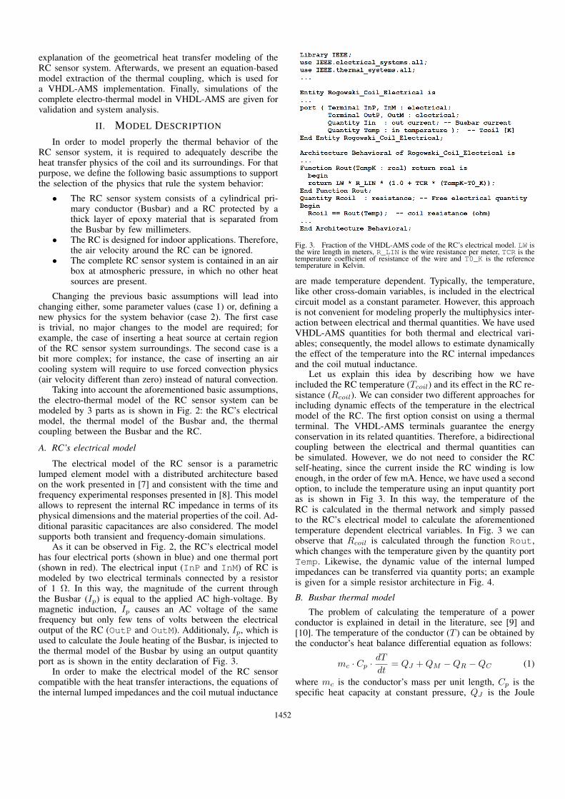
In order to explain how and where Tcoil is defined, let usconsider Fig. 9. This is a steady-state simulation of the SHTmodel in which is plotted the temperature throughout a cutlinefrom the Busbar surface (distance = 0 m) to the extreme ofthe air box. The cutline is taken at the RC geometrical centeras is shown in Fig. 5b. The distances a, b, c and d in Fig. 9correspond to the highlighted distances in Fig. 5b. It can beobserved that the temperature decrement is significantly fasterin the air region than inside the RC, i.e. the region betweena and b. In a closer look in Fig. 9b, we can see that thetemperature remains practically constant throughout the RC

(a) Overall view (b) Zoom

Fig. 8. Tcoil (C) vs. Time (hours), CHT and SHT transient simulation.Tbus = 100C, Troom = 25C, Agap = 4.2mm.

1454

(a) (b)

Fig. 9. Temperature (C) vs. Distance (m). SHT static simulation throughoutthe cutline shown in Fig. 5b. (a) Entire region. (b) Zoom in the RC region.

core, i.e. the region between c and d. Actually, the temperatureinside the RC core also decreases with the distance to theBusbar surface. However, the temperature difference betweenthe inner and the outer extreme of the RC core is less thanfew tens of mili-Celsius. Therefore, we can safely define Tcoilas the temperature at any point inside c and d.

C. Equation-based model of the thermal coupling

From the transient behavior of the CHT/SHT model, wecan estimate the transient behavior of Tcoil using the followingEquation:

Tcoil(t) = T0 + (TSS − T0)

(1− e−

tτ

)(6)

where T0 is the effective initial temperature of the RC, TSSis the final steady-state temperature of the RC, and τ is thetime constant of the RC sensor. The SHT model can be usedfor static parametric simulations to obtain TSS at differentconditions. Afterwards, a polynomial curve fitting algorithmis performed to obtain the following equation:

TSS(Tbus, Troom, Agap) = P0 + P1Tbus + P2Troom+P3Agap (7)

where Pi are fitting coefficients which depends on the RC coreused.

Likewise, an equation for τ can also be acquired by poly-nomial curve fitting. However, τ can only be obtained by tran-sient simulations. Consequently, its estimation by parametricsimulation is highly time consuming and impractical. A goodapproximation for the time behavior of the thermal couplingmodel can be made by considering an average (avg) or aworst case scenario, i.e. to simulate the maximum (max) andminimum (min) τ of the system within the sweep parameterrange shown in TABLE 1. After a series of simulations, it hasbeen observed that τ is highly dependent on Agap, and slightlydependent on Tbus and Troom; therefore, τ is approximated asfollows:

τx(Agap) = S3A3gap + S2A

2gap + S1Agap + S0 (8)

where Si are fitting coefficients which depends on the RC coreused and the considered case (i.e. x = min / avg / max).

Name Min Max Step

Tbus -5 C 200 C 5 C

Troom -10 C 90 C 5 C

Agap 0 mm 5 mm 0.2 mm

TABLE 1. SWEEP PARAMETER RANGE.

D. Electro-Thermal Model Simulation and Analysis

By parametric static and transient simulations of the geo-metrical SHT model, we can get an equation-based model ofthe thermal coupling by using equations 2, 3 and 4. Afterwards,the model of the Electro-Thermal RC sensor system (ETRCS)shown in Fig. 2 can be completed in VHDL-AMS. It is worthmentioning that this model only fits a particular selection ofRC dimensions and materials.

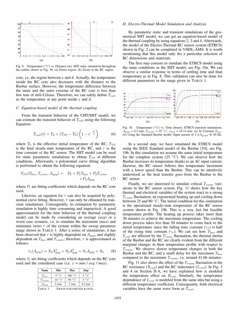
The first step consists to simulate the ETRCS model usingthe same conditions as the SHT model, see Fig. 10a. We canobserve a similar response in terms of settling time and finaltemperature as in Fig. 8. This validation can also be done fordifferent parameters in the range given in TABLE 1.

(a) (b)

Fig. 10. Temperature (C) vs. Time (hours), ETRCS transient simulations.Agap = 4.2 mm, Troom = 25 C, τavg = 34.14 min. (a) At Constant Tbus.(b) Using the Standard Busbar model: Input current of 2 kApeak @ 50 Hz.

In a second step, we have simulated the ETRCS modelusing the IEEE Standard model of the Busbar [10], see Fig.10b. In this simulation we assume the same initial temperaturefor the complete system (25 C). We can observe how theBusbar increases its temperature thanks to an AC input current;likewise, the RC sensor follows this temperature incrementwith a lower speed than the Busbar. This can be intuitivelyunderstood as the heat transfer goes from the Busbar to theRC sensor.

Finally, we are interested to simulate critical Troom vari-ations in the RC sensor system. Fig. 11 shows how the keythermal and electrical variables of the system react to a strongTroom fluctuation, an exponential heating up and cooling downbetween 25 and 80 C. The initial condition for this simulationis the operational steady-state temperature of the RC sensorsystem shown in Fig. 10b. This is a very fast but feasibletemperature profile. The heating up process takes more than30 minutes to achieve the maximum temperature. The coolingdown process takes less than 50 minutes to come back to theinitial temperature since the falling time constant (γf ) is halfof the rising time constant (γr). We can see how Tbus andTcoil are affected by the Troom fluctuation, the thermal inertiaof the Busbar and the RC are clearly evident from the differentmarginal changes in their temperature profile with respect toTroom. We observe slower temperature changes in both theBusbar and the RC, and a small delay for the maximum Tbuscompared to the maximum Troom, i.e. around 41.66 minutes.

Fig. 11 also shows the effect of the Troom fluctuation in theRC resistance (Rcoil) and the RC inductance (Lcoil). In Fig. 3and 4 on Section II-A, we have explained how is modeledthe temperature effect on Rcoil. Similarly, the temperaturedependence of Lcoil is modeled from the same idea but using adifferent temperature coefficient. Consequently, both electricalvariables have the same wave form as Tcoil.

1455

Fig. 11. ETRCS transient simulation. Vertical axes: Temperature (uppergraph), Inductance (middle graph), Resistance (bottom graph). Exponentialtime constants for Troom: γr = 500 sec (rising), γf = 1000 sec (falling).Initial temperature condition: Tbus = 105.9C, Tcoil = 88.9C andTroom = 25C.

In order to quantify the effect of the Troom variation on theelectrical variables, we can define the relative variable changeas follows:

∆M =(Mmax −Mmin)

Mmin∗ 100 (9)

where M is the specific electrical variable. In Fig. 11, therelative Rcoil change (∆Rcoil) is about 14%, whereas therelative Lcoil change (∆Lcoil) is only about 0.0992%. Thissignificative difference is mainly due to we have used insimulation a temperature coefficient of inductance (TCL) twoorders of magnitude lower than the temperature coefficient ofresistance of cooper (TCR = 0.0039 K−1).

This type of simulation can be used to test the systemunder different room temperature conditions. Although theETRCS model can give results for divergent Troom profiles,it is important to consider realistic fluctuations in terms ofvariation speed and wave form. This is especially importantto validate this model by using experimental measurements.Moreover, non-commercial RC applications, in which verylow temperatures might appear in the system (such as in[11]), could benefit from this co-design methodology betweenVHDL-AMS and FEA. However, it is important to know thevalidity range of the thermal and electrical models. Furthermodifications to the physics and other assumptions in themodel can be done for studies under extreme temperatureconditions.

IV. CONCLUSION

We exploit the multi-domain capabilities of VHDL-AMStogether with geometrical FEA to create a versatile parametricmodel, which can be used for both thermal and electricalsimulations. We further improve a classical lumped-elementelectrical model of the Rogowski Coil to support the dynamiceffect of temperature. We show that the proposed electro-thermal model can estimate dynamically the internal tempera-ture of the coil and its dependency on geometrical, electricaland thermal parameters of the system. Furthermore, the modelis able to simulate critical temperature fluctuations in the sys-tem caused by room temperature drifts. This is very importantfor a better understanding of the temperature effects in the

electrical variables of the sensor and the direct implication inits signal processing electronics. Both electrical and thermalmeasurements are required for a complete validation of themodel here proposed.

REFERENCES

[1] W. Ray and C. Hewson, “High performance rogowski current trans-ducers,” in Conference Record of the 2000 IEEE Industry ApplicationsConference, 2000, vol. 5, 2000, pp. 3083–3090 vol.5.

[2] M. Samimi, A. Mahari, M. Farahnakian, and H. Mohseni, “Therogowski coil principles and applications: A review,” IEEE SensorsJournal, vol. 15, no. 2, pp. 651–658, Feb. 2015.

[3] A. Marinescu, “A calibration laboratory for rogowski coil used in energysystems and power electronics,” in 2010 12th International Conferenceon Optimization of Electrical and Electronic Equipment (OPTIM), May2010, pp. 913–919.

[4] G. Meijer, M. Pertijs, and K. Makinwa, Smart Sensor Systems: Emerg-ing Technologies and Applications. Delft University of Technology,the Netherlands: John Wiley and Sons, May 2014.

[5] M. Zhang, K. Li, S. He, and J. Wang, “Design and test of a newhigh-current electronic current transformer with a rogowski coil,”Metrology and Measurement Systems, vol. 21, no. 1, pp. 121–132,2014. [Online]. Available: http://www.degruyter.com/view/j/mms.2014.21.issue-1/mms-2014-0012/mms-2014-0012.xml

[6] H. Wang, F. Liu, H. Zhang, and S. Zheng, “Analysis of the thermalexpansion effect on measurement precision of rogowski coils,” inInternational Conference on Power Electronics and Drives Systems,2005. PEDS 2005, vol. 2, 2005, pp. 1658–1661.

[7] V. Dubickas and H. Edin, “High-frequency model of the rogowski coilwith a small number of turns,” IEEE Transactions on Instrumentationand Measurement, vol. 56, no. 6, pp. 2284–2288, 2007.

[8] E. Hemmati and S. Shahrtash, “Investigation on rogowski coil perfor-mance for structuring its design methodology,” IET Science, Measure-ment Technology, vol. 7, no. 6, pp. 306–314, Nov. 2013.

[9] P. Nefzger, U. Kaintzyk, and J. F. Nolasco, Overhead Power Lines:Planning, Design, Construction. Springer, Apr. 2003.

[10] IEEE Power Engineering Society, “IEEE standard for calculating thecurrent-temperature of bare overhead conductors,” IEEE-SA StandardsBoard, Standard IEEE Std 738-2006, Nov. 2006.

[11] P. Moreau, A. Le-Luyer, P. Malard, P. Pastor, F. Saint-Laurent,P. Spuig, J. Lister, M. Toussaint, P. Marmillod, D. Testa, S. Peruzzo,J. Knaster, G. Vayakis, S. Hughes, and K. M. Patel, “Prototyping andtesting of the continuous external rogowski ITER magnetic sensor,”Fusion Engineering and Design, vol. 88, no. 6–8, pp. 1165–1169,Oct. 2013. [Online]. Available: http://www.sciencedirect.com/science/article/pii/S0920379612005777

1456

Powered by TCPDF (www.tcpdf.org)